Rethinking Nearest Neighbors for Visual Classification

Abstract

Neural network classifiers have become the de-facto choice for current “pre-train then fine-tune” paradigms of visual classification. In this paper, we investigate $k$-Nearest-Neighbor ($k$-NN) classifiers, a classical model-free learning method from the pre-deep learning era, as an augmentation to modern neural network based approaches. As a lazy learning method, $k$-NN simply aggregates the distance between the test image and top-$k$ neighbors in a training set. We adopt $k$-NN with pre-trained visual representations produced by either supervised or self-supervised methods in two steps: (1) Leverage $k$-NN predicted probabilities as indications for easy vs. hard examples during training. (2) Linearly interpolate the $k$-NN predicted distribution with that of the augmented classifier. Via extensive experiments on a wide range of classification tasks, our study reveals the generality and flexibility of $k$-NN integration with additional insights: (1) $k$-NN achieves competitive results, sometimes even outperforming a standard linear classifier. (2) Incorporating $k$-NN is especially beneficial for tasks where parametric classifiers perform poorly and / or in low-data regimes. We hope these discoveries will encourage people to rethink the role of pre-deep learning, classical methods in computer vision.

1 Introduction

Deep neural networks revolutionized computer vision, and have become a fundamental tool for a wide variety of applications. With the advancement of representation learning, it is now common practice to leverage the features extracted from large-scaled labeled data (e.g., ImageNet [13]), or other pretext tasks (e.g., colorization [78, 79], rotations of inputs [22], modeling image similarity and dissimilarity among multiple views [31, 9, 8, 4, 10, 76, 5], to name a few), and transfer them to target domains, such as object detection [24, 23, 55, 32], action recognition [56, 6], or various fine-grained recognition tasks [11, 58, 64, 18].

Eager learners [20], like neural networks, require an intensive learning stage to estimate the model parameters. Thus the majority of computation occurs at training time. A stark contrast to deep neural networks is the $k$-Nearest Neighbor ($k$-NN) classifier: a classical, “old-school” learning method. As a lazy learning approach, $k$-NN requires no learning / training time. It simply memorizes training data and predicts labels based on the nearest training examples. $k$-NN also avoids over-fitting of parameters [1] and is robust to input perturbations [50]. Because of the favorable properties of $k$-NN, researchers (e.g. [77, 1, 15, 69, 70, 68, 27]) periodically revisit $k$-NN each time new paradigms of eager learners emerge, raising the questions: what role remains for this simple non-parametric learning approach? Is “good old” $k$-NN still useful, or should it be relegated to historical background sections in pattern recognition textbooks?

In this paper, we investigate how to incorporate the complementary strengths of nearest neighbors and neural network methods for current “pre-train then fine-tune” paradigms of visual classification. Our work builds upon recent findings that self-supervised Vision Transformer features enable excellent $k$-NN classification [5]. We further demonstrate that all features, regardless of the pre-training backbones or objectives, can benefit from $k$-NN. Using the embedded visual representations as input, we propose to leverage the predictive results of a $k$-NN classifier and augment conventional modern classifiers in two steps: (1) During training, we treat $k$-NN results as an indication of easy vs. hard examples in the training set. More specifically, we add a scaling factor to the standard cross-entropy criterion of conventional classifiers, automatically forcing the model to focus on the hard examples identified by $k$-NN. (2) During test time, we linearly interpolate probability distributions from the learned augmented model with the distributions produced by $k$-NN.

Extensive experiments show that incorporating $k$-NN improves standard parametric classifiers results across a wide range of classification tasks. In addition, we observe the following: (1) $k$-NN can be on par with neural network models, sometimes surpassing linear classifier counterparts. (2) Leveraging $k$-NN is especially helpful for tasks beyond object classification and in low-data regimes. These findings reveal that the $k$-NN classifier, which is “rarely appropriate for use,” is still valuable in the deep learning era. Our work makes the following key contributions:

1. A simple yet effective approach to augment standard neural network methods with $k$-NN in both training and inference stages. We show that integrating $k$-NN in both stages is more robust than integrating during test time only as proposed in previous work [57, 28, 50, 38, 37].

2. An extensive evaluation of the role of $k$-NN in the context of a wide variety of classification tasks and experimental setups, demonstrating the flexibility and generality of integrating $k$-NN.

We hope this work can broaden the landscape of computer vision and inspire future research that rethinks the role of old-school methods.

2 Related Work

$k$-NN in the era of deep learning

While $k$-NN has declined in visibility relative to modern neural network based approaches in the last decade or so, it did not fall completely off the radar. A $k$-NN based model was shown to provide strong baselines for image captioning [14, 15], image restoration [54], few-shot learning [68], and evaluation of representation learning [66, 5]. Nearest-Neighbor approaches are also used for improving interpretability and robustness of models against adversarial attacks [51, 50, 36], language modeling [28, 38], machine translation [63, 37], and learning a finer granularity than the one provided by training labels [62]. The notion of building associations and differentiating data instances has also been used in self-supervised learning [69, 70, 8, 31, 9, 10, 4, 76]. Most recently, Granot et al. [27] describe a patch-based nearest neighbors approach for single image generative models, producing more realistic global structure and less artifacts. In this paper, we seek to explore how to augment existing neural network models with $k$-NN, where the relative notion of similarity is based on the representations of the images.

Hybrid approach of eager and lazy learning

Our work can be seen as a continuation of a line of work that combines eager learners with lazy learners [57, 28, 50, 47, 38, 37, 41]. Eager learners, such as neural networks, are trained to provide a global approximating function that maps from input to output space. Lazy learners, on the contrary, focus on approximating the neighborhoods around test examples [2]. To leverage the “best of both worlds,” researchers have adopted simple interpolation strategies to combine these models. The predictive results from $k$-NN are linearly interpolated with those of an eager learner, either by a fixed scalar [57, 28, 50, 38, 37] or a learned weight [47]. Our present work takes a step further for fruitful pairings: in addition to the aforementioned approach, we propose to train a parametric classifier with the predictive results of $k$-NN as guidance so the learned classifier will focus more on the examples misclassified by $k$-NN.

Transfer learning

Transfer learning [7] has always been one of the “tricks of the trade” of machine learning practitioners. It has been widely used for evaluating representation learned under weakly-supervised [59, 60, 46, 39, 40, 42, 34], semi-supervised [73, 74, 71] and self-supervised learning paradigms [70, 3, 80, 16, 75, 4, 29, 31, 48, 8, 43, 76, 12]. Transfer learning exploits the associations between the pre-trained task and the target task, especially when the data in the target task is scarce and high-capacity deep neural networks suffer from overfitting. In this work, we utilize the transfer learning settings and use the visual representation learned from target task as input for $k$-NN classifier.

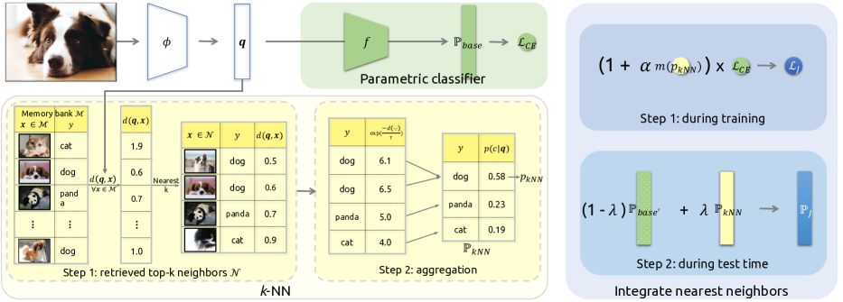
Figure 1: Method overview. Left: comparison between a parametric classifier and a $k$-NN classifier. Right: Given an image, we integrate $k$-NN classifier results to augment the conventional parametric classifier in two stages: (1): During training, we utilize $k$-NN results as an indication of easy vs. hard instances and rescale the loss accordingly; (2): During test time, we linear interpolate results of two classifiers with a tunable parameter $\lambda$. Note we use the predicted results from the classifier learned using $\mathcal{L}_{J}$ from step 1. See texts for more details.

3 Approach

Our goal is to investigate the role of the $k$-Nearest-Neighbor ($k$-NN) classifier in the era of deep learning. Let $\phi$ be a visual feature extractor that transforms an input image $I$ into a numerical representation with dimensions $D$: $\mathbf{x}=\phi(I)\in\mathds{R}^{D}$. $\mathbf{x}$ are used as input for $k$-NN, which we describe in Sec. 3.1. We then introduce our method to integrate $k$-NN with standard parametric classifiers in Sec. 3.2. The overall framework is presented in Fig. 1.

3.1 Nearest neighbors revisited

$k$-Nearest-Neighbor ($k$-NN) classifiers require no model to be fit. Given a set of $n$ labeled images, we have the corresponding set of features $\mathcal{M}=\{\mathbf{x}_{1},\dots,\mathbf{x}_{n}\}$, and a set of target labels $\{y_{1},\dots,y_{n}\}$, $y\in[1,C]$. Given a representation $\mathbf{q}=\phi(I_{q})$ of a new image example $I_{q}$, $k$-NN classifier can be described in the following two steps:

Step 1: Retrieve $k$ neighbors

We first compute the Euclidean distance between the query $\mathbf{q}$ and all the examples in $\mathcal{M}$: $d(\mathbf{q},\mathbf{x})$, $\forall\mathbf{x}\in\mathcal{M}$. Then a set of $k$ representations are selected, which are the closest in distance to $\mathbf{q}$ in the embedded space. As commonly practiced in $k$-NN (e.g., [20, 70, 68]), we pre-process both $\mathbf{q}$ and features of $\mathcal{M}$ with $l2$-normalization and subtracting the mean across $\mathcal{M}$ ($\mathbf{\mu}=\frac{1}{n}\sum_{\mathbf{x}\in\mathcal{M}}\mathbf{x}$) from each feature.

Step 2: Aggregation

Let $\mathcal{N}$ be the retrieved set of top-$k$ neighbors, and $\mathcal{N}_{c}$ be the subset of $\mathcal{N}$ where all examples have the same class $c$. The top-$k$ neighbors to $\mathbf{q}$ and their corresponding targets are converted into a distribution over $C$ classes. The probability of $\mathbf{q}$ being predicted as $c$ is:

$$p_{k\text{NN}}(c|\mathbf{q})=\frac{\sum_{\mathbf{x}\in\mathcal{N}_{c}}\exp{}\left(-d(\mathbf{q},\mathbf{x})/\tau\right)}{\sum_{c\in C}\sum_{\mathbf{x}\in\mathcal{N}_{c}}\exp{}\left(-d(\mathbf{q},\mathbf{x})/\tau\right)}\;\;.$$ (1)

where $\tau$ is a temperature hyper-parameter. Higher $\tau$ produces a softer and more flattened probability distribution.

Comparing to parametric classifiers

Given $\mathbf{q}$ and $C$ target classes, the probability of being predicted by a conventional parametric softmax classifier as target $c$ is

$$p(c|\mathbf{q})=\frac{\exp{f_{c}(\mathbf{q})}}{\sum_{i=1}^{C}\exp{f_{i}(\mathbf{q})}}\;\;,{}$$ (2)

where $f_{i}(\cdot)$ is a parametric function that measures how well $\mathbf{q}$ matches the $i^{\text{th}}$ target class. In the example of a linear classifier $f(\mathbf{q})=W\mathbf{q}+\mathbf{b}$. The key difference to $k$-NN is $\{W,\mathbf{b}\}$, which are parameters learned with a set of labeled training data.

3.2 Integrating nearest neighbors

Leveraging the lazy learning benefits of $k$-NN, we propose to augment the parametric classifier in both the training and test stages.

Step 1: Integrating during training

Since $k$-NN’s predictions given $\mathbf{q}$ can be easily computed, we wish to guide the network to attend to difficult examples during training. In particular, we use $k$-NN results to differentiate between easy vs. hard examples. Given a $k$-NN probability of the ground-truth class $p_{k\text{NN}}$, we rescale the standard cross-entropy loss $\mathcal{L}_{CE}$ to adjust the relative loss for the misclassified or well-classified instances identified by $k$-NN, respectively. We employ the negative log-likelihood as the modulating factor $m(p_{k\text{NN}})$. The final loss $\mathcal{L}_{J}$ is defined as:

$$m(p_{k\text{NN}})=-\log{}(p_{k\text{NN}})\;\;,$$ (3)

$$\mathcal{L}_{J}=\left(1+\alpha m(p_{k\text{NN}})\right)\mathcal{L}_{CE}\;\;,$$ (4)

$\alpha$ is a scalar to determine the contribution of each loss term.

Note we use training set as $\mathcal{M}$. Each example cannot retrieve itself as a neighbor. Thus $p_{k\text{NN}}$ is computed using the leave-one-out distribution on the training set [69]. Furthermore, the idea of using a modulating factor to reweight loss of easy vs. hard examples can be found in modern neural networks literature [44]. Interestingly, we will show by experiments (Sec. 5) that our proposed loss is not sensitive to the initiation of modulating factor, indicating that utilizing $k$-NN predictions during training is the main reason for the observed improvements in Secs. 4, 5 and 6.

Step 2: Integrating during test time

Let $\mathbb{P}_{\text{{Base}${}^{\prime}${}}}$ be the predicted class distribution produced by the trained classifier from Step 1, and $\mathbb{P}_{k\text{NN}}$ be that of a $k$-NN classifier. We calculate the final probability distribution $\mathbb{P}_{J}$ as:

$$\mathbb{P}_{J}=\lambda\mathbb{P}_{k\text{NN}}+(1-\lambda)\mathbb{P}_{\text{{Base}${}^{\prime}${}}}\;\;,$$ (5)

where $\lambda\in[0,1]$ is a tuned hyper-parameter. Since the $k$-NN distribution assigns non-zero probability to at most $k$ classes, Eq. 5 also ensures non-zero probability over the entire classes.

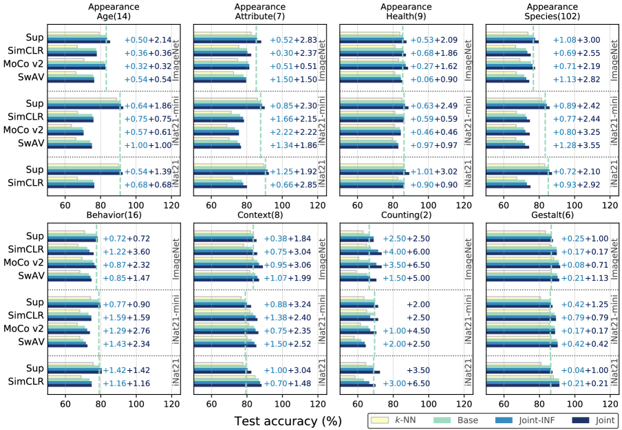
Figure 2: Results on NeWT. Every experiment uses ResNet-50 as pre-training backbone. The y-axis denotes the pre-training objectives while the text on the right specify the pre-training datasets. Performance gains of Joint-inf and Joint for each representation are presented if applicable. The green dashed line in each subplot represent the Base results with supervised feature extractors.

4 Experiments

We conduct extensive experiments using three sets of classification tasks with benchmarking datasets, comparing the performance of methods that incorporate $k$-NN, with conventional parametric classifier and $k$-nearest neighbor classifier. We first describe our experimental setup (Sec. 4.1), and demonstrate the effectiveness of our integrated methods on natural world binary classification [64] (Sec. 4.2), fine-grained object classification [65, 49, 52, 21] (Sec. 4.3) and ImageNet classification [13] (Sec. 4.4).

4.1 Evaluation protocols and details

We adopt linear evaluation as it is a common feature representation evaluation protocol [46, 26, 48, 31]. Pre-trained models are used as visual feature extractors, where the weights of the image encoders are fixed. We compare the proposed method (denote as Joint) with the following approaches: (1) Base: which is the vanilla linear classifier, whose performance usually indicates how effective the learned representations are; (2) $k$-NN described in Sec. 3.1; (3) Joint-inf: which simply linear interpolate $k$-NN and Base result during test time.

We experiment with a wide range of feature representations, categorized by its (1) pre-trained objectives, (2) pre-trained datasets, and (3) feature backbones. We consider 8 different training objectives including Supervised (Sup) setting and self-supervised objectives: SimCLR [8], MoCo v2 [31, 9], MoCo v3 [10], SwAV [4], BarlowTwins [76], DINO [5], MoBY [72]. The pre-training datasets can be either ImageNet [13] or iNaturalist2021 (iNat2021) [64]. The feature backbones include ResNet [33], Vision Transformers (ViT) [17] and Swin Transformer (Swin [45]). Appendix B provides more implementation details, including an itemized list of the feature representations configurations, dataset specifications, and a full list of hyperparameters used (batch sizes, learning rates, decay schedules, etc.).

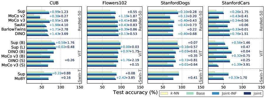
Figure 3: Results on fine-grained down-stream datasets. All features are pre-trained on ImageNet. The y-axis denotes the pre-training objectives while the text on the right specify the feature extractor backbones. We also include the performance gains of Joint and Joint-inf for each representation evaluated if applicable.

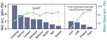
Figure 4: Relative average accuracy gain ($\%$) vs. average Base accuracy rate ($\%$) across all the evaluated features for NeWT and fine-grained object classification tasks.

4.2 Natural world binary classification

Settings

We first evaluate the effect of integrating $k$-NN on a collection of Natural World Tasks (NeWT) [64]. It comprises 164 binary classification tasks related to different aspects of natural world images, including appearances, behavior, context, counting, and gestalt. Following [64], we categorize the tasks into 8 coarse groups and report the mean test accuracy score of each group. In addition to features pre-trained on ImageNet and iNat2021, we also report the features pre-trained on a randomly sampled subset (18.6 $\%$) of iNat2021, denoted as iNat2021-mini. Fig. 2 summarizes the experimental results. Sec. A.4 includes the accuracy values for all tasks.

Results

Fig. 2 shows that Joint noticeably surpasses the vanilla linear classifier counterpart (Base) for all 8 groups of NeWT and all the feature representations evaluated. In general, relative accuracy gains and Base results are negatively correlated. Fig. 4 summarizes this trend. For example, we observe non-trivial performance gains of both Joint-inf and Joint on the counting task: +5.2$\%$ / +9.7$\%$ relative gains over base (67.0$\%$) for Joint-inf (70.5$\%$) and Joint (73.5$\%$), respectively, using supervised pre-training methods on iNat2021. This task group receives the lowest mean Base accuracy across all features (66.5$\%$) among NeWT, suggesting Joint is more effective on the poorly performing parametric classifiers.

4.3 Fine-grained object classification

Settings

We further demonstrate the effect of Joint by benchmarking fine-grained object classification tasks: Caltech-UCSD Birds-200-2011 (CUB-200-2011 [65]), Oxford Flowers [49], Stanford Dogs [52], Stanford Cars [21]. All four datasets are multi-class classification tasks. If a certain dataset only has train and test set publicly available, we randomly split the training set into train (90%) and val (10%) and optimize the top-$1$ accuracy scores on val to select hyperparameters. Sec. B.2 includes additional information about these tasks. Fig. 3 presents the test accuracy rate for the test set of these datasets. All feature representations are pre-trained on ImageNet.

Results

From Fig. 3, we can see that: (1) Joint offers better or comparable results than the linear classifier counterpart. (2) Joint is more generalizable than Joint-inf. For ResNet-50 backbone, Joint achieves accuracy gains over all the features across four datasets, while Joint-inf brings reduced improvement over a subset of the evaluated features. We observe that Joint-inf sometimes can be prone to overfitting, where val results are higher yet test results are not. (3) Comparing to NeWT, we see a similar trend where the improvement of Joint is negatively correlated with Base results. See Fig. 4 (right). (4) Joint achieves higher accuracy gains on ResNet backbone in general, comparing with other transformer-based backbones (ViT and Swin). This could suggest that the transferability of ResNet features is not fully exploited using a linear classifier alone.

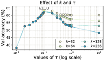
(a) Effect of $\tau$.

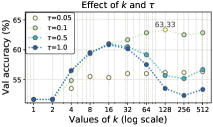
(b) Effect of $k$.

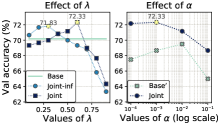
(c) Effect of $\lambda$ and $\alpha$.

Figure 5: Tuning $k$-NN and Joint-inf and Joint. (a,b): Effect of $k,\tau$ on the $k$-NN accuracy scores. (c): Effect of interpolating factor $\lambda$ on Joint-inf and $\alpha$ on Joint accuracy scores. All results are for CUB-200-2011 val dataset with supervised imageNet pre-training ResNet-50 backbone.

4.4 ImageNet classification

Settings

We evaluate the image classification task using ImageNet (ILSVRC 2012) [13], which contains 1.3 million training and 50k validation natural scene images with 1000 classes. For supervised objectives, we freeze the feature extractors and re-initiate the last layer for the Joint approach. Tab. 1 summarizes the results with top-1 accuracy rate.

Backbone	Pre-trained Objective	Top 1 Accuracy ($\%$)
		$k$-NN	Base	Joint-inf	Joint
ResNet-50	Supervised	72.65	76.01	($\uparrow$0.37) 76.39	($\uparrow$0.50) 76.52
	MoCo v3 [10]	68.51	73.88	($\uparrow$1.25) 75.13	($\uparrow$1.28) 75.16
	SwAV [4]	68.54	⋆74.63	($\uparrow$1.48) 76.11	($\uparrow$1.40) 76.04
	BarlowTwins [76]	67.85	⋆72.88	($\uparrow$1.52) 74.40	($\uparrow$1.31) 74.18
	DINO [5]	68.40	⋆74.38	($\uparrow$1.60) 75.97	($\uparrow$1.54) 75.91
ViT-B/16	Supervised [17]	77.27	75.70	($\uparrow$1.78) 77.48	($\uparrow$2.62) 78.32
ViT-L/16	Supervised [17]	80.25	79.20	($\uparrow$1.21) 80.41	($\uparrow$1.61) 80.81
ViT-S/16	MoCo v3 [10]	69.01	⋆73.33	($\uparrow$1.25) 74.58	($\uparrow$1.23) 74.56
ViT-B/16	MoCo v3 [10]	72.24	⋆76.35	($\uparrow$1.02) 77.38	($\uparrow$1.05) 77.41
Swin-T	Supervised [45]	80.06	⋆80.98	($\uparrow$0.25) 81.23	($\uparrow$0.25) 81.23
	MoBY [72]	68.87	⋆74.68	($\uparrow$0.84) 75.52	($\uparrow$0.91) 75.59

Table 1: Results on ImageNet. All features are pre-trained on ImageNet. Base results with ^⋆ are run by us. ($\cdot$) indicates the difference to Base. Methods that incorporate nearest neighbors consistently outperform the Base and $k$-NN counterparts.

Results

Under both protocols (Joint-inf and Joint), integrating nearest neighbors achieves consistently better performance for ImageNet than Base across three backbone choices and all the pre-training objectives. Comparing with Joint results, we observe that Joint-inf offers comparable performance, sometimes even outperforms Joint by a slight margin (0.06-0.21) for ImageNet experiments. This is different from the previous two experiments in Secs. 4.2 and 4.3, suggesting that Joint is more suitable for downstream tasks that possibly have larger domain shift than the pre-trained dataset. Note that we use in-house Base results for fair-comparison with Joint. Some Base results are different (within 1$\%$) from the reported results from prior work. Sec. A.4 includes experiments with the released linear classifiers’ weights.

5 Analysis

To better understand the proposed integration approach, we conduct ablation studies and qualitative analysis using CUB-200-2011. We define Base^′ as the classifier trained with $\mathcal{L}_{J}$ of Eq. 4 without test time integration. More results and analysis are included in the Appendix A.

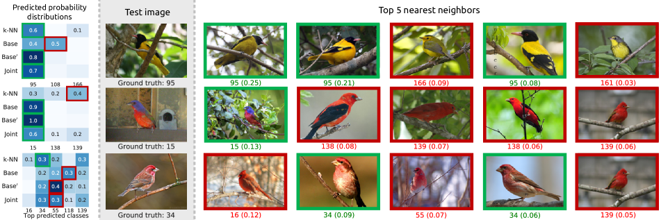
Figure 6: Qualitative results where $k$-NN and Base produce different predictions. We show the predicted probability distribution (left), the test image (middle), and the top-5 nearest neighbors from the training set on the right. Only predicted probabilities $>0.1$ are presented in the left due to space constraint. Title of each retrieved samples follows the format: class index( $\exp{\left(-d(\cdot,\cdot)/\tau\right)}$ from Eq. 1 ).

Modulating factor initiations

In previous experiments, we use negative log-likelihood (NLL) as a function of $k$-NN predicted probability. The modulating factor is used to weight samples based on $k$-NN prediction quality during training. A relatively modern method (comparing to $k$-NN which was first proposed in 1951 [19]) to instance-based weighting is focal loss [44], which proposes to weight training samples with $(1-p)^{\gamma}$, where $p$ is the ground-truth class probability produced by a parametric classifier. Like NLL, this initiation also reduces the relative loss for well-classified examples. See Appendix A for visualization and further analysis of both modulating factor choices.

We thus adopt focal loss modulating factor as an alternative initiation for Joint: $(1-p_{k\text{NN}})^{\gamma}$. We train Joint with focal weighting strategy (Joint-Focal) using identical settings as before on CUB-200-2011 and report the results in Tab. 2. Joint-Focal achieves nearly the same accuracy as those trained with negative log-likelihood (Joint-NLL). Both weighting strategies for Joint improve vanilla linear classifier performance by up to 7$\%$, suggesting that the exact form of modulating factor is not crucial. A similar finding was also discussed in [44]. Joint-Focal is a reasonable alternative for Joint-NLL and works well in practice.

Pre-trained Objective	Top 1 Accuracy ($\%$)
	Base	Joint-NLL	Joint-Focal	$\alpha$	$\gamma$
Supervised	68.48	($\uparrow$1.23) 69.71	($\uparrow$1.47) 69.95	0.001	2
MoCo v3 [10]	69.76	($\uparrow$1.09) 70.85	($\uparrow$1.04) 70.80	0.0001	0.5
SwAV [4]	58.53	($\uparrow$4.10) 62.63	($\uparrow$3.91) 62.44	0.01	0.5
BarlowTwins [76]	63.12	($\uparrow$2.78) 65.90	($\uparrow$2.86) 65.98	0.001	2
DINO [5]	64.41	($\uparrow$3.69) 68.10	($\uparrow$3.61) 68.02	0.01	0.5

Table 2: Negative log-likelihood vs. focal loss weight factors comparison. All features are pre-trained on ImageNet with ResNet-50. ($\cdot$) indicates the difference to Base. The differences between both weighting schemes are within 0.35$\%$ of each other.

Tuning $k$-NN

Figs. 5(a) and 5(b) present the effect of number of nearest neighbors considered ($k$) and temperature value ($\tau$ from Eq. 1) on the val accuracy score of CUB-200-2011. Fig. 5(a) shows that $k$-NN achieves better performance as $\tau$ increases up to $0.1$. $\tau=0.01$ produces over-concentrated distribution and makes the model overfit to the most similar retrievals. $\tau>0.1$ can deteriorate the performance through over-smoothing the probability distribution and increasing the entropy [67]. Fig. 5(b) shows that for a fixed temperature value, the performance does not always improve using a larger $k$ since more nearest neighbors retrieved will likely include more instances with wrong labels. Combinations of larger values of $\tau$ (e.g. $\tau>0.1$) and larger $k$ ($k\geq 16$) will lead to even further reduced $k$-NN accuracy rates. The effect of $k$ diminishes gradually as $\tau$ decreases (e.g. $\tau=0.05$).

Tuning Joint

To investigate the effect of how much the model relies on $k$-NN, we also ablate the linear interpolation parameter $\lambda$ in Eq. 5 and the scaling factor $\alpha$ in Eq. 4. Fig. 5(c) summarizes the results. Fig. 5(c) (left) shows that the optimal $\lambda$ increases for Joint comparing to Joint-inf, as the model relies more on $k$-NN with a specific weighting loss during training. Fig. 5(c) (right) shows that the optimal values of $\alpha$ are different between the linear classifier learned under Joint framework (Base^′) and Joint ($0.001$ and 0.01, respectively), highlighting the fact that the linear classifier that is complementary to $k$-NN is not always the best performing classifier.

Qualitative Analysis

To further understand the role of $k$-NN and the benefit of Joint, we manually inspect cases in which Base and $k$-NN produce different predictions with $\phi(\cdot)$ being the supervised pre-training on ImageNet. Fig. 6 shows such examples, along with others in the Appendix. For each test example, we plot the predicted probability distributions of Joint and other approaches ($k$-NN, Base, Base^′ which is the linear classifier trained with $k$-NN weighted loss in Eq. 4). Top 5 nearest neighbors from the train split of CUB-200-2011 are also visualized at the right hand side of the figure. $k$-NN can produce correct predictions when Base fails, especially when Base produces high entropy distributions (top and bottom cases). Via reweighting the easy vs. hard examples identified by the $k$-NN results, Base^′ produces a larger probability for the correct class in all three cases. However, the bottom row shows that Joint and Base^′ produces incorrect result even when $k$-NN is correct, possibly due to the existence of 5 fine-grained classes. The visual representation (input for $k$-NN) seems not discriminative enough to distinguish the subtle differences among these classes.

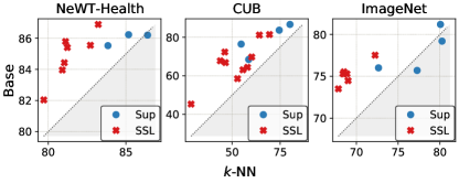
Figure 7: Supervised (Sup) vs. self-supervised (SSL) features perform differently between $k$-NN (x-axis) and Base (y-axis). Each point represents accuracy rate of one feature configuration from Figs. 2 and 3, and Tab. 1.

6 Discussion

Rethinking $k$-NN and visual representations

Our experiments show that in addition to features learned with a self-supervised ViT backbone, visual representations of diverse specifications (pre-training objectives, dataset, and backbones) can produce competitive $k$-NN results. This observation expands the findings of Caron et al. [5]. In particular, the relative accuracy between Base and $k$-NN varies across pre-training objectives; see Fig. 7. The supervised pre-training features are more favorable for $k$-NN in general. The performance gap between $k$-NN and Base is smaller for these supervised features.

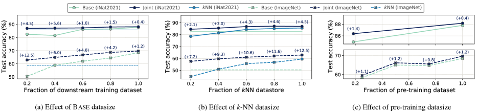
Figure 8: Dataset size ablation results with CUB-200-2011. We study how the amount of data used for (a) Base, (b) $k$-NN, and (c) pre-training process affects the performance. We use full $k$-NN data for (a), 20$\%$ Base data for (b), full $k$-NN and Base data for (c). (a-b) use full pre-training data. All experiments use ResNet-50 as backbone. Legend follows format: method (pre-training data). ($\cdot$) denotes the differences between Joint and Base under each variation.

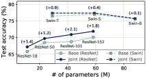
(a) Effect of pre-training backbone.

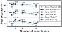
(b) Effect of downstream MLP sizes.

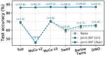
(c) Effect of $k$-NN features.

Figure 9: Backbone architectures ablation results. We change the architectures of the (a) feature extractors, (b) Base classifier, and (c) $k$-NN feature extractors. All results are for CUB-200-2011 test split with supervised pre-training objectives on ImageNet. Fig. 9(c) uses ResNet-50. ($\cdot$) denotes the differences to Base under each variation.

Joint is helpful in low-data regimes

Next, we analyze the impact of the proposed method when varying the size (by random sampling) of (1) Base training data, (2) $k$-NN datastore, (3) labeled pre-training dataset using supervised pre-training methods with both ImageNet and iNat2021. Fig. 8 summarizes the results. Increasing the downstream data or $k$-NN datastore sizes monotonically improves the performance of Joint. We also observe that with a better feature extractor (using iNat2021 as pre-training dataset in this case), Joint is more robust to data size variation: (1) using 60$\%$ of data for either Base (Fig. 8a) or $k$-NN (Fig. 8b), Joint can achieve comparable results with the counterparts that use the full data, and (2) with less than 20$\%$ of iNat2021, Joint could nearly match the Base results using the full pre-training data (Fig. 8c).

Joint consistently outperforms Base over different pre-training backbone choices

Fig. 9(a) shows ablation results using different pre-training backbone architectures. Joint is better than Base across all backbone choices. We also note that the advantages of Joint do not diminish as the number of parameters of backbone gets larger for ResNet based backbones, yet diminish for Swin (possibly due to overfitting on the downstream training set.)

Joint generalizes well to Base beyond linear classifier

A natural question to ask is instead of the proposed method, what if we simply use a better classifier? We investigate this by increasing the single linear classifier to a multilayer perceptron (MLP) and varying the number of layers ($\{2,4,8\}$). We report the results of Base and Joint of three different feature extractors in Fig. 9(b). We can see that the performance gains of Joint extend to multiple layers, even for MLP with 8 layers where the Base is overfitting on the training set.

Better $k$-NN features result in larger performance gains

We also ablate on the features used for $k$-NN and report Joint-inf results in Fig. 9(c). We choose the supervised pre-training method on iNat2021 since it transfers better to CUB-200-2011 as shown in Fig. 8 and achieves 86$\%$ top-1 accuracy with $k$-NN. The results show that further improvements may be possible by only swapping $k$-NN features, suggesting that rather than re-train a new linear classifier with the improved feature representations, we can change the $k$-NN datastore and save learning / training time.

Limitations

In this paper, we use a vanilla implementation of $k$-NN, which will incur large computational overhead when dealing with billions of training images. One possible solution is to use implementations such as FAISS [35] for fast nearest neighbor search in high dimensional spaces.

The generality and flexibility of integrating $k$-NN

In this work, we propose to augment standard neural network classifiers with $k$-NN. Our results reveal a number of important benefits of incorporating $k$-NN. In terms of generality, we observe improved performance in every experimental setup: low vs. high data regimes used for pre-training, Base, or $k$-NN; different architecture choices of Base (linear vs. MLP); and classification tasks (binary vs. multi-class, fine-grained vs. standard ImageNet, species vs. other natural world tasks). In terms of flexibility, our hybrid approach is effective with diverse visual representations ranging from supervised to self-supervised methods, from ResNet to ViT and Swin, from pre-trained on ImageNet to iNat2021. We therefore hope our work could inspire and facilitate future research that reconsiders the role of the classical methods with the continuous advancement of the field.

Acknowledgement

This work is supported by a Meta AI research grant awarded to Cornell University.

Appendix A Supplementary Results and Discussion

We provide the following items that shed further insight on the effect of $k$-NN and the proposed $k$-NN integration method:

• Further analysis of Sec. 5 from the main text (Sec. A.1);

• An extended discussion of the benefit of $k$-NN and societal impact (Sec. A.2);

• Ablations experiments on the design choices of $k$-NN (Sec. A.3);

• Supplementary empirical results of $k$-NN integration (Secs. A.4 and A.5).

Unless otherwise specified, all the experimental results of this section are on CUB-200-2011 test set, using the supervised representations pre-trained on ImageNet with ResNet-50 backbone.

A.1 Further analysis of $k$-NN integration

Modulating factor initiations We visualize both modulating factor initiations (negative log-likelihood (NLL) and focal loss (Focal)) from Sec. 5 in Fig. 10 with selected settings of $\alpha$ and $\gamma$. NLL gives more weight for $p_{k\text{NN}}<0.1$. Given the predicted distribution of $k$-NN is sparser than Base (see Figs. 6 and 11 for examples), NLL produces larger weights for the misclassified examples. This could be the reason why NLL variant performs slightly better than Focal in Tab. 2.

More qualitative results Fig. 11 presents more test examples of CUB-200-2011 where $k$-NN and Base disagree with each other. By explicitly memorizing the training data, $k$-NN can produce correct predictions when Base produces low confidence false positives. Fig. 11 also demonstrates the effect of proposed joint loss $\mathcal{L}_{J}$: the augmented linear classifier (Base^′) creates higher confidence predictions compared to Base.

A.2 Extended discussion

Joint is robust to hyper-parameter tuning Fig. 12 presents performance of Base and Joint with different values of learning rate and weight decay. As can be seen, Joint achieves relatively similar accuracy rates with a wide range of learning rates and weight decay values. This suggests that by incorporating $k$-NN, the proposed method can be robust to the hyperparameters of Base, hence potentially reducing the range of grid search and increasing model development efficiency.

The complementary effect of Base and $k$-NN As discussed in the main text, $k$-NN has complementary strengths when compared to the neural network methods (lazy vs. eager learners). Sections 4, 5 and 6 present extensive empirical results to demonstrate that our proposed hybrid approach outperforms the Base and $k$-NN counterparts. We further examine the complementary strengths of both learning methods by plotting per-class Precision-Recall (PR) curves for CUB-200-2011 in Fig. 13. Figs. 13(a) and 13(b) show $k$-NN reaches higher recalls without any false positive predictions, while Figs. 13(c) and 13(d) present two cases where Base performs better.

Societal impact This paper investigates the role of “old-school” methods ($k$-NN) in the era of the deep-learning revolution. Given a photo, the proposed method predicts probability distribution based on both learned global and local statistics in the training set, from the neural network and $k$-NN, respectively. Thus the learned statistics could reflect and amplify potential biases in the training data, such as selection, framing and labeling biases [61]. We would like to raise awareness of such issues. Any machine learning down-stream tasks should always apply fairness into consideration during algorithm development. Note previous works have shown another benefit of $k$-NN: improving interpretability [51, 50, 36]. This suggests that integrating $k$-NN could potentially help down-stream applications towards responsible and ethical machine learning practices.

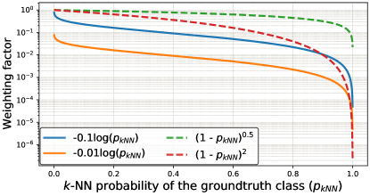
Figure 10: Visualizations of both negative log-likelihood (NLL) and focal loss (Focal) variants with different settings of $\alpha$ and $\gamma$. Both variants reduce the relative loss for well-classified examples.

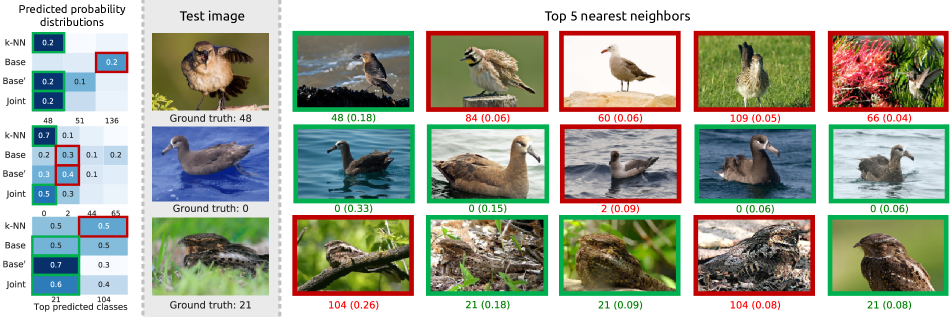
Figure 11: Additional results where $k$-NN and Base produce different predictions. We show the predicted probability distribution (left), the test image (middle), and the top-5 nearest neighbors from the training set on the right. Only predicted probability $>0.1$ are presented in the left due to space constraint. Title of each retrieved samples follow the format: class index ($\exp{\left(-d(\cdot,\cdot)/\tau\right)}$ from Eq. 1)

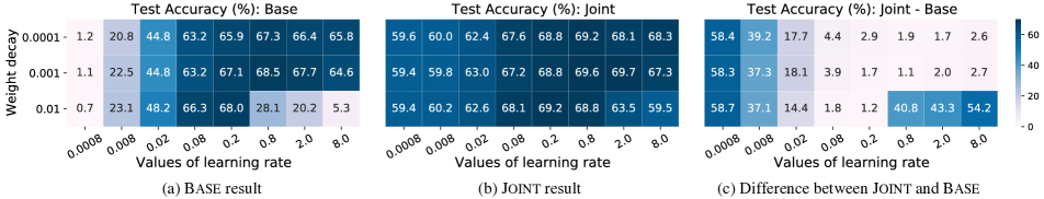
Figure 12: Base, Joint and Joint - Base performance over different values of learning rate and weight decay using CUB-200-2011. Joint is robust to hyperparameter tuning.

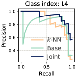
(a)

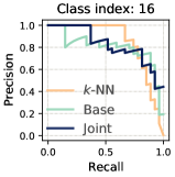
(b)

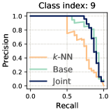
(c)

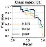
(d)

Figure 13: Precision-Recall (PR) curves of four classes in CUB-200-2011. Base and $k$-NN have complementary strength.

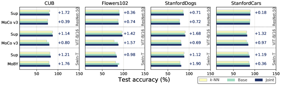
Figure 14: Fine-tuning results on the fine-grained down-stream datasets. All features are pre-trained on ImageNet. The y-axis denotes the pre-training objectives while the text on the right specify the feature extractor backbones. We also include the performance gains of Joint compare to Base for each representation evaluated if applicable.

A.3 Other design choices of $k$-NN

We present the preliminary experiments that lead to the design choices we made for the $k$-NN classifier described in Sec. 3.1. We report the accuracy rate (%) of CUB-200-2011 test split.

Does the similarity metric of $k$-NN matter? We use the negative squared Euclidean distance ($-d_{L2}$) to measure the similarity between the query $\mathbf{q}$ and examples in the memory bank $\mathcal{M}$. Another common metric is cosine similarity ($d_{cos}$), which is commonly used in the contrastive self-supervised learning literature ([31, 5], to name a few). We present $k$-NN performance using both metrics with hyperparameters $k,\tau$ below.

Similarity metric	$-d_{L2}$	$d_{cos}$
Accuracy (%)	63.67	63.33
$k$	128	128
$\tau$	0.06	0.1

Both similarity metrics lead to near the same $k$-NN classification results with different optimal $\tau$, possibly due to the fact that both metrics are related with the $l_{2}$ normalized features ($-d_{L2}=2d_{cos}-2$). We thus adopt $-d_{L2}$ in the main text, expecting similar performance with $d_{cos}$.

ResNet-based features: which down-sampling method to use? We experiment on different pooling methods for ResNet-based features: (1) MaxPool, (2) AvgPool, (3) R-MAC [25] (4) None: we simply flatten the feature map. The following are the $k$-NN classification results, showing that MaxPool outperforms the other pooling variants.

Pooling method	MaxPool	AvgPool	R-MAC	None
Accuracy (%)	63.67	55.07	60.56	47.96

ResNet-based features: which layer’s information to use as $\mathbf{x}$? We use the MaxPool-ed feature maps from the last convolutional block of ResNet-50 as input $\mathbf{x}$ for $k$-NN. The table below shows the $k$-NN accuracy with feature maps from different convolutional blocks of ResNet-50.

Conv blocks	1	2	3	4	5
Accuracy (%)	6.23	9.51	19.26	35.47	63.67

$k$-NN performs the best when using the last feature map as input, as a deep neural network close to the output layer contain holistic semantic information of the image [50].

A.4 Additional results

Numerical results of NeWT and fine-grained recognition experiments The project page includes tables presenting full empirical results including performance on the val split and corresponding hyper-parameters used ($\tau,k,\alpha,\lambda$, learning rate, and weight decay). These files can be read in conjunction with the figures and tables in the main text (Figs. 2, 3, 1, 8 and 9). Note that we use in-house baselines instead of copying results from prior work for fair-comparison purposes. All the experiments are trained using the same grid search range, validation set, learning rate schedule, input augmentation schemes etc. See Appendix B for details.

ImageNet results with the off-the-shelf Base We report results of in-house Base for fair comparison across all feature configurations in Sec. 4.4. For completeness, we additionally compare the $k$-NN integration (during test time only) with off-the-shelf ImageNet classifiers. Tab. 3 summarizes the results. As can be seen, incorporating $k$-NN in test time outperforms the vanilla neural network based classifier counterpart across all the evaluated features.

Backbone	Pre-trained Objective	Top 1 Accuracy ($\%$)
		$k$-NN	Base	Joint-inf
ResNet-50	Supervised	72.65	76.01	($\uparrow$0.37) 76.39
	MoCo v3 (ep100)	61.97	68.96	($\uparrow$1.06) 70.02
	MoCo v3 (ep300)	66.51	72.87	($\uparrow$0.99) 73.86
	MoCo v3 (ep1000)	67.33	74.57	($\uparrow$0.96) 75.53
ViT-B/16	MoCo v3	71.22	76.61	($\uparrow$0.91) 77.52
ViT-S/16	MoCo v3	67.55	73.33	($\uparrow$1.15) 74.48

Table 3: Results on ImageNet using the off-the-shelf weights.

A.5 End-to-end fine-tuning

Settings We additionally run experiments under fine-tuning transfer learning protocol, where we use the pre-trained models as initiations for the four fine-grained object classification tasks [49, 65, 52, 21]. The parameters of the feature extractors $\phi(\cdot)$ are modified during training. We thus update the memory bank $\mathcal{M}$ of $k$-NN every epoch for Joint method. Similar to experiments in Sec. 4.3, we use either publicly available or randomly sampled val set to select hyperparameters. All feature representations are pre-trained on ImageNet.

Results Fig. 14 presents the test set accuracy rates of $k$-NN, Base, Joint. We observe that Joint could improve the vanilla neural network model. For example, Joint achieves 1.72 $(2.17\%)$ accuracy gain using imagenet supervised representations with ResNet-50 backbone.

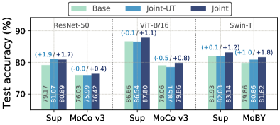
Figure 15: Effect of updating memory bank. The x-axis denotes the pre-training objectives while the text on the top specify the feature extractor backbones. We also include the difference of Joint-ut and Joint compared to Base for each representation evaluated.

Updating $\mathcal{M}$ Under the fine-tuning protocol, we update the memory bank $\mathcal{M}$ every epoch to reflect the change of the feature extractor. We additionally experiment on a variant Joint-ut: Updating $\mathcal{M}$ during Test time only. In particular, we use the pre-trained features for $\mathcal{M}$ during the end-to-end training, and the updated features during test time. Fig. 15 presents the results on CUB-200-2011. Updating $\mathcal{M}$ every epoch (Joint) generalizes better than Joint-ut. Considering its slight computational advantage, Joint-ut may be preferred in cases where it is desirable to trade off a certain amount of accuracy for the reduced training time. e.g., for the CUB-200-2011 dataset, Joint-ut takes around 6 hours (20.8%) less than Joint with the Swin-T supervised ImageNet pre-training features when trained on a single A100 GPU using our PyTorch implementation.

Appendix B Reproducibility Details

B.1 Implementation details

We use Pytorch [53] to implement and train all the models on NVIDIA Tesla V100 and A100-40GB GPUs, for pre-training and transfer learning experiments, respectively. We adopt standard image augmentation strategy during training (randomly resize crop to 224 $\times$ 224 and random horizontal flip). Other implementation details are described below and the specific hyper-parameter values for each experiment can be found in the project page mentioned in Sec. A.4.

Modulating factor of $\mathcal{L}_{J}$ Similar to pytorch’s BCELoss, we clamp the $log$ function outputs to be greater than or equal to -100, so we can always have a finite value of the modulating factor. Tab. 4 presents the range of other hyper-parameters used for $k$-NN and Joint.

Transfer learning settings Since the dataset is not balanced, we follow [44] to stabilize the training processing by initializing the the bias for the last linear classification layer with $b=-\log\left(\left(1-\pi\right)/\pi\right)$, where the prior probability $\pi$ is set to 0.01. Tabs. 5 and 6 summarize the optimization configurations we used. Following [46], we conduct a coarse grid search to find the learning rate and weight decay values using val split. The learning rate is set as $\text{Base LR}/256\times b$, where $b$ is the batch size used for the particular model, and Base LR is chosen from the range specified in Tabs. 5 and 6.

Pre-training settings We additionally trained three supervised ResNet-50 models using subsets of ImageNet. These models are trained on 8 GPUs. We use a batch size of 1024 images, stochastic gradient descent with a momentum of 0.9, and a weight decay of 0.0001. The base learning rate is set according to $0.1/256\times b$, where $b$ is the batch size used for the particular model. The learning rate is warmed up linearly from 0 to the base learning rate during the first $5\%$ of the whole iterations, then reduced by a factor of $0.1$ during epoch $\{30,60,90\}$.

B.2 Datasets and feature representations

The statistics of the evaluated tasks and the associated datasets are shown in Tab. 7. Features of NeWT are obtained from the researchers who propose the datasets. Tab. 8 enumerates all the features we used in the main text.

Config	Values
$k$	$\{2^{\{0:1:9\}},mean\}$
$\tau$	$\{$0.001, 0.01, 0.1, 1, 10,
	$0.01\times\{1:1:10\},0.1\times\{1:1:10\}$ $\}$
$\alpha$	$\{0.01,0.001,0.0001\}$
$\lambda$	$\{0.50:.05:0.95\}$

Table 4: Joint setting. $mean$ represents the average image count per class for different tasks.

Config	Value
optimizer	SGD
base LR range	$\{$0.5, 0.25, 0.1, 0.05, 0.025,
	0.01, 0.0025, 0.001 $\}^{\star}$
weight decay range	$\{0.01,0.001,0.0001,0.0\}$
optimizer momentum	0.9
learning rate schedule	cosine decay
warm up epochs	10
total epochs	100

Table 5: Linear evaluation setting. ^⋆For the self-supervised features, we use a different range for base learning rate: $\{40,20,10,5.0,2.5,1.0,0.5,0.05,0.1\}$ since the feature magnitudes are different from the supervised variants. Note that we can alternatively add a normalization layer before the linear classifier following [30] instead of using larger learning rate values.

Config	Value
optimizer	SGD
base LR range	$\{$0.05, 0.025, 0.005,
	0.0025, 0.0005, 0.00025 $\}$
weight decay range	$\{0.01,0.001,0.0001,0.00001\}$
optimizer momentum	0.9
learning rate schedule	cosine decay
warm up epochs	5
total epochs	300

Table 6: End-to-end fine-tuning evaluation setting.

Dataset	Description	# Classes	Train	Val	Test	License with links
ImageNet [13]	Image recognition	1,000	1,281,167	50,000	-	Non-commercial
Caltech-UCSD Birds-200-2011 [65]	Fine-grained bird species recognition	200	5,394⋆	600⋆	5,794	Non-commercial
Oxford Flowers [49]	Fine-grained flower species recognition	102	1,020	1,020	6,149	Not specified
Stanford Dogs [52]	Fine-grained dog species recognition	120	10,800⋆	1,200⋆	8,580	Not specified
Stanford Cars [21]	Fine-grained car detection	196	7,329⋆	815⋆	8,041	Non-commercial
Natural World Tasks (NeWT) [64]	A set of 196 natural world classification tasks					Non-commercial
Appearance-Age	14 binary tasks	2	114.29 $\pm$ 34.99	-	114.29 $\pm$ 34.99
Appearance-Attribute	7 binary tasks	2	97.71 $\pm$ 5.60	-	87.43 $\pm$ 24.85
Appearance-Health	9 binary tasks	2	122.22 $\pm$ 41.57	-	116.44 $\pm$ 45.15
Appearance-Species	102 binary tasks	2	97.29 $\pm$ 25.93	-	100.12 $\pm$ 25.19
Behavior	16 binary tasks	2	100.00 $\pm$ 0.00	-	88.06 $\pm$ 18.10
Context	8 binary tasks	2	100.00 $\pm$ 0.00	-	105.50 $\pm$ 25.82
Counting	2 binary tasks	2	100.00 $\pm$ 0.00	-	100.00 $\pm$ 0.00
Gestalt	6 binary tasks	2	350.00 $\pm$ 111.80	-	349.83 $\pm$ 111.73

Table 7: Specifications of the various datasets evaluated. Image number with ^⋆ are the subset we randomly sampled since no publicly data splits are available. We report mean and standard deviation of data sizes for NeWT. “Non-commercial” is short for “non-commercial research and educational purposes only”.

Pre-trained Backbone	Pre-trained Objective	Pre-trained Data	Throughput (img/s)	# params (M)	Feature dim	Batch Size	Pre-trained Model
ResNet-50 [33]	Supervised	ImageNet [13]	1581.6	23	2048	2048 / 384	link
		ImageNet-25$\%$ [13]					in house
		ImageNet-50$\%$ [13]					in house
		ImageNet-75$\%$ [13]					in house
		iNaturalist2021 (iNat) [64]					link
		iNaturalist2021-mini (iNat-mini) [64]					link
ResNet-18 [33]		ImageNet [13]	4602.5	11	2048	2048 / -	link
ResNet-101 [33]		ImageNet [13]	963.6	43			link
ResNet-152 [33]		ImageNet [13]	685.0	58			link
ResNet-50 [33]	MoCo v2 [9]	ImageNet [13]	1581.6	23	2048	2048 / 384	link
	MoCo v3 [10]						link
	SwAV [4]						link
	DINO [5]						link
	BarlowTwins [76]						link
ViT-B/16 [17]	Supervised	ImageNet [13]	1264.7	85	768	1024 / 192	link
ViT-L/16 [17]			460.2	307	1024	512 / -	link
ViT-S/16 [17]	DINO [5]	ImageNet [13]	2342.0	21	384	1024 / -	link
ViT-S/16 [17]	MoCo v3 [10]		2342.0	21	384	1024 / -	link
ViT-B/16 [17]	DINO [5]		1264.7	85	768	1024 / -	link
ViT-B/16 [17]	MoCo v3 [10]		1264.7	85	768	1024 / 192	link
Swin-T [45]	Supervised	ImageNet [13]	1438.3	29	768	1024 / 192	link
Swin-S [45]			946.8	50	768	1024 / -
Swin-B [45]			716.9	88	1024	1024 / -
Swin-T [45]	MoBY [72]	ImageNet [13]	1438.2	29	768	1024 / 192	link

Table 8: Specifications of different representation learning approaches ($\phi(\cdot)$) evaluated for fine-grained object recognition and ImageNet classification tasks. All features are pre-trained with an randomly resized cropped input image of size 224$\times$224. The throughput (im/s) is calculated on a NVIDIA A100 GPU. Parameters (M) are of the feature extractor. Batch size column reports the batch size for linear evaluation and fine-tuning experiments, respectively. See Sec. B.1 and attached CSV files for more implementation details.

References

- [1] Oren Boiman, Eli Shechtman, and Michal Irani. In defense of nearest-neighbor based image classification. In CVPR, pages 1–8. IEEE, 2008.
- [2] Gianluca Bontempi, Hugues Bersini, and Mauro Birattari. The local paradigm for modeling and control: from neuro-fuzzy to lazy learning. Fuzzy sets and systems, 121(1):59–72, 2001.
- [3] Mathilde Caron, Piotr Bojanowski, Armand Joulin, and Matthijs Douze. Deep clustering for unsupervised learning of visual features. In ECCV, 2018.
- [4] Mathilde Caron, Ishan Misra, Julien Mairal, Priya Goyal, Piotr Bojanowski, and Armand Joulin. Unsupervised learning of visual features by contrasting cluster assignments. In NeurIPS, 2020.
- [5] Mathilde Caron, Hugo Touvron, Ishan Misra, Hervé Jégou, Julien Mairal, Piotr Bojanowski, and Armand Joulin. Emerging properties in self-supervised vision transformers. In ICCV, 2021.
- [6] Joao Carreira and Andrew Zisserman. Quo vadis, action recognition? a new model and the kinetics dataset. In CVPR, pages 6299–6308, 2017.
- [7] Rich Caruana. Multitask learning. Machine learning, 28(1):41–75, 1997.
- [8] Ting Chen, Simon Kornblith, Mohammad Norouzi, and Geoffrey Hinton. A simple framework for contrastive learning of visual representations. In ICML, pages 1597–1607. PMLR, 2020.
- [9] Xinlei Chen, Haoqi Fan, Ross Girshick, and Kaiming He. Improved baselines with momentum contrastive learning. arXiv preprint arXiv:2003.04297, 2020.
- [10] Xinlei Chen*, Saining Xie*, and Kaiming He. An empirical study of training self-supervised vision transformers. In ICCV, 2021.
- [11] Yin Cui, Yang Song, Chen Sun, Andrew Howard, and Serge Belongie. Large scale fine-grained categorization and domain-specific transfer learning. In CVPR, pages 4109–4118, 2018.
- [12] Zhiyuan Dang, Cheng Deng, Xu Yang, Kun Wei, and Heng Huang. Nearest neighbor matching for deep clustering. In CVPR, pages 13693–13702, 2021.
- [13] Jia Deng, Wei Dong, Richard Socher, Li-Jia Li, Kai Li, and Li Fei-Fei. Imagenet: A large-scale hierarchical image database. In CVPR, 2009.
- [14] Jacob Devlin, Hao Cheng, Hao Fang, Saurabh Gupta, Li Deng, Xiaodong He, Geoffrey Zweig, and Margaret Mitchell. Language models for image captioning: The quirks and what works. In Proceedings of the 53rd Annual Meeting of the Association for Computational Linguistics and the 7th International Joint Conference on Natural Language Processing (Volume 2: Short Papers), pages 100–105, Beijing, China, July 2015. Association for Computational Linguistics.
- [15] Jacob Devlin, Saurabh Gupta, Ross Girshick, Margaret Mitchell, and C Lawrence Zitnick. Exploring nearest neighbor approaches for image captioning. arXiv preprint arXiv:1505.04467, 2015.
- [16] Jeff Donahue and Karen Simonyan. Large scale adversarial representation learning. In NeurIPS, 2019.
- [17] Alexey Dosovitskiy, Lucas Beyer, Alexander Kolesnikov, Dirk Weissenborn, Xiaohua Zhai, Thomas Unterthiner, Mostafa Dehghani, Matthias Minderer, Georg Heigold, Sylvain Gelly, et al. An image is worth 16x16 words: Transformers for image recognition at scale. In ICLR, 2020.
- [18] Linus Ericsson, Henry Gouk, and Timothy M Hospedales. How well do self-supervised models transfer? In CVPR, pages 5414–5423, 2021.
- [19] Evelyn Fix. Discriminatory analysis: nonparametric discrimination, consistency properties, volume 1. USAF School of Aviation Medicine, 1985.
- [20] Jerome H Friedman. The elements of statistical learning: Data mining, inference, and prediction. springer open, 2017.
- [21] Timnit Gebru, Jonathan Krause, Yilun Wang, Duyun Chen, Jia Deng, and Li Fei-Fei. Fine-grained car detection for visual census estimation. In AAAI, 2017.
- [22] Spyros Gidaris, Praveer Singh, and Nikos Komodakis. Unsupervised representation learning by predicting image rotations. In ICLR, 2018.
- [23] Ross Girshick. Fast r-cnn. In ICCV, pages 1440–1448, 2015.
- [24] Ross Girshick, Jeff Donahue, Trevor Darrell, and Jitendra Malik. Rich feature hierarchies for accurate object detection and semantic segmentation. In CVPR, pages 580–587, 2014.
- [25] Albert Gordo, Jon Almazan, Jerome Revaud, and Diane Larlus. End-to-end learning of deep visual representations for image retrieval. IJCV, 124(2):237–254, 2017.
- [26] Priya Goyal, Dhruv Mahajan, Abhinav Gupta, and Ishan Misra. Scaling and benchmarking self-supervised visual representation learning. In ICCV, pages 6391–6400, 2019.
- [27] Niv Granot, Ben Feinstein, Assaf Shocher, Shai Bagon, and Michal Irani. Drop the gan: In defense of patches nearest neighbors as single image generative models. arXiv preprint arXiv:2103.15545, 2021.
- [28] Edouard Grave, Moustapha Cissé, and Armand Joulin. Unbounded cache model for online language modeling with open vocabulary. In NeurIPS, 2017.
- [29] Jean-Bastien Grill, Florian Strub, Florent Altché, Corentin Tallec, Pierre Richemond, Elena Buchatskaya, Carl Doersch, Bernardo Avila Pires, Zhaohan Guo, Mohammad Gheshlaghi Azar, Bilal Piot, koray kavukcuoglu, Remi Munos, and Michal Valko. Bootstrap your own latent - a new approach to self-supervised learning. In H. Larochelle, M. Ranzato, R. Hadsell, M. F. Balcan, and H. Lin, editors, NeurIPS, pages 21271–21284, 2020.
- [30] Kaiming He, Xinlei Chen, Saining Xie, Yanghao Li, Piotr Dollár, and Ross Girshick. Masked autoencoders are scalable vision learners. arXiv preprint arXiv:2111.06377, 2021.
- [31] Kaiming He, Haoqi Fan, Yuxin Wu, Saining Xie, and Ross Girshick. Momentum contrast for unsupervised visual representation learning. In CVPR, pages 9729–9738, 2020.
- [32] Kaiming He, Georgia Gkioxari, Piotr Dollár, and Ross Girshick. Mask r-cnn. In ICCV, pages 2961–2969, 2017.
- [33] Kaiming He, Xiangyu Zhang, Shaoqing Ren, and Jian Sun. Deep residual learning for image recognition. In CVPR, pages 770–778, 2016.
- [34] Menglin Jia, Zuxuan Wu, Austin Reiter, Claire Cardie, Serge Belongie, and Ser-Nam Lim. Exploring visual engagement signals for representation learning. In ICCV, 2021.
- [35] Jeff Johnson, Matthijs Douze, and Hervé Jégou. Billion-scale similarity search with gpus. IEEE Transactions on Big Data, 2019.
- [36] Jake Zhao (Junbo) and Kyunghyun Cho. Retrieval-augmented convolutional neural networks against adversarial examples. In CVPR, June 2019.
- [37] Urvashi Khandelwal, Angela Fan, Dan Jurafsky, Luke Zettlemoyer, and Mike Lewis. Nearest neighbor machine translation. In ICLR, 2021.
- [38] Urvashi Khandelwal, Omer Levy, Dan Jurafsky, Luke Zettlemoyer, and Mike Lewis. Generalization through memorization: Nearest neighbor language models. In ICLR, 2020.
- [39] Alexander Kolesnikov, Lucas Beyer, Xiaohua Zhai, Joan Puigcerver, Jessica Yung, Sylvain Gelly, and Neil Houlsby. Large scale learning of general visual representations for transfer. arXiv preprint arXiv:1912.11370, 2019.
- [40] Alexander Kolesnikov, Lucas Beyer, Xiaohua Zhai, Joan Puigcerver, Jessica Yung, Sylvain Gelly, and Neil Houlsby. Big transfer (bit): General visual representation learning. In ECCV, 2020.
- [41] David Leake, Xiaomeng Ye, and David J Crandall. Supporting case-based reasoning with neural networks: An illustration for case adaptation. In AAAI Spring Symposium: Combining Machine Learning with Knowledge Engineering, 2021.
- [42] Junnan Li, Caiming Xiong, and Steven Hoi. Mopro: Webly supervised learning with momentum prototypes. In ICLR, 2021.
- [43] Junnan Li, Pan Zhou, Caiming Xiong, and Steven Hoi. Prototypical contrastive learning of unsupervised representations. In ICLR, 2021.
- [44] Tsung-Yi Lin, Priya Goyal, Ross Girshick, Kaiming He, and Piotr Dollár. Focal loss for dense object detection. In CVPR, 2018.
- [45] Ze Liu, Yutong Lin, Yue Cao, Han Hu, Yixuan Wei, Zheng Zhang, Stephen Lin, and Baining Guo. Swin transformer: Hierarchical vision transformer using shifted windows. In ICCV, 2021.
- [46] Dhruv Mahajan, Ross Girshick, Vignesh Ramanathan, Kaiming He, Manohar Paluri, Yixuan Li, Ashwin Bharambe, and Laurens Van Der Maaten. Exploring the limits of weakly supervised pretraining. In ECCV, 2018.
- [47] Fei Mi and Boi Faltings. Memory augmented neural model for incremental session-based recommendation. arXiv preprint arXiv:2005.01573, 2020.
- [48] Ishan Misra and Laurens van der Maaten. Self-supervised learning of pretext-invariant representations. In CVPR, 2020.
- [49] Maria-Elena Nilsback and Andrew Zisserman. Automated flower classification over a large number of classes. In 2008 Sixth Indian Conference on Computer Vision, Graphics & Image Processing, pages 722–729. IEEE, 2008.
- [50] Emin Orhan. A simple cache model for image recognition. NeurIPS, 31:10107–10116, 2018.
- [51] Nicolas Papernot and Patrick McDaniel. Deep k-nearest neighbors: Towards confident, interpretable and robust deep learning. arXiv preprint arXiv:1803.04765, 2018.
- [52] Omkar M Parkhi, Andrea Vedaldi, Andrew Zisserman, and CV Jawahar. Cats and dogs. In CVPR, pages 3498–3505. IEEE, 2012.
- [53] A. Paszke, S. Gross, S. Chintala, G. Chanan, E. Yang, Z. DeVito, Z. Lin, A. Desmaison, L. Antiga, and A. Lerer. Automatic differentiation in PyTorch. In NeurIPS Autodiff Workshop, 2017.
- [54] Tobias Plötz and Stefan Roth. Neural nearest neighbors networks. In NeurIPS, 2018.
- [55] Shaoqing Ren, Kaiming He, Ross Girshick, and Jian Sun. Faster r-cnn: Towards real-time object detection with region proposal networks. NeurIPS, 28:91–99, 2015.
- [56] Karen Simonyan and Andrew Zisserman. Two-stream convolutional networks for action recognition in videos. In NeurIPS, pages 568–576, 2014.
- [57] Dimitri P Solomatine, Mahesh Maskey, and Durga L Shrestha. Eager and lazy learning methods in the context of hydrologic forecasting. In The 2006 IEEE International Joint Conference on Neural Network Proceedings, pages 4847–4853. IEEE, 2006.
- [58] Jong-Chyi Su, Subhransu Maji, and Bharath Hariharan. When does self-supervision improve few-shot learning? In ECCV, pages 645–666. Springer, 2020.
- [59] Chen Sun, Abhinav Shrivastava, Saurabh Sigh, and Abhinav Gupta. Revisiting unreasonable effectiveness of data in deep learning era. In ICCV, 2017.
- [60] Bart Thomee, David A Shamma, Gerald Friedland, Benjamin Elizalde, Karl Ni, Douglas Poland, Damian Borth, and Li-Jia Li. YFCC100M: The new data in multimedia research. Communications of the ACM, 2016.
- [61] Antonio Torralba and Alexei A Efros. Unbiased look at dataset bias. In CVPR, pages 1521–1528. IEEE, 2011.
- [62] Hugo Touvron, Alexandre Sablayrolles, Matthijs Douze, Matthieu Cord, and Hervé Jégou. Grafit: Learning fine-grained image representations with coarse labels. In ICCV, pages 874–884, 2021.
- [63] Zhaopeng Tu, Yang Liu, Shuming Shi, and Tong Zhang. Learning to remember translation history with a continuous cache. Transactions of the Association for Computational Linguistics, 6:407–420, 2018.
- [64] Grant Van Horn, Elijah Cole, Sara Beery, Kimberly Wilber, Serge Belongie, and Oisin Mac Aodha. Benchmarking representation learning for natural world image collections. In CVPR, pages 12884–12893, June 2021.
- [65] Catherine Wah, Steve Branson, Peter Welinder, Pietro Perona, and Serge Belongie. The caltech-ucsd birds-200-2011 dataset. Technical Report CNS-TR-2011-001, California Institute of Technology, 2011.
- [66] Bram Wallace and Bharath Hariharan. Extending and analyzing self-supervised learning across domains. In ECCV, pages 717–734. Springer, 2020.
- [67] Feng Wang and Huaping Liu. Understanding the behaviour of contrastive loss. In CVPR, pages 2495–2504, 2021.
- [68] Yan Wang, Wei-Lun Chao, Kilian Q Weinberger, and Laurens van der Maaten. Simpleshot: Revisiting nearest-neighbor classification for few-shot learning. arXiv preprint arXiv:1911.04623, 2019.
- [69] Zhirong Wu, Alexei A Efros, and Stella X Yu. Improving generalization via scalable neighborhood component analysis. In ECCV, pages 685–701, 2018.
- [70] Zhirong Wu, Yuanjun Xiong, Stella X Yu, and Dahua Lin. Unsupervised feature learning via non-parametric instance discrimination. In CVPR, pages 3733–3742, 2018.
- [71] Qizhe Xie, Minh-Thang Luong, Eduard Hovy, and Quoc V. Le. Self-training with noisy student improves imagenet classification. In CVPR, 2020.
- [72] Zhenda Xie, Yutong Lin, Zhuliang Yao, Zheng Zhang, Qi Dai, Yue Cao, and Han Hu. Self-supervised learning with swin transformers. arXiv preprint arXiv:2105.04553, 2021.
- [73] I Zeki Yalniz, Hervé Jégou, Kan Chen, Manohar Paluri, and Dhruv Mahajan. Billion-scale semi-supervised learning for image classification. arXiv preprint arXiv:1905.00546, 2019.
- [74] Xueting Yan, Ishan Misra, Abhinav Gupta, Deepti Ghadiyaram, and Dhruv Mahajan. Clusterfit: Improving generalization of visual representations. In CVPR, pages 6509–6518, 2020.
- [75] Mang Ye, Xu Zhang, Pong C Yuen, and Shih-Fu Chang. Unsupervised embedding learning via invariant and spreading instance feature. In CVPR, 2019.
- [76] Jure Zbontar, Li Jing, Ishan Misra, Yann LeCun, and Stéphane Deny. Barlow twins: Self-supervised learning via redundancy reduction. CoRR, abs/2103.03230, 2021.
- [77] Hao Zhang, Alexander C Berg, Michael Maire, and Jitendra Malik. Svm-knn: Discriminative nearest neighbor classification for visual category recognition. In CVPR, volume 2, pages 2126–2136. IEEE, 2006.
- [78] Richard Zhang, Phillip Isola, and Alexei A Efros. Colorful image colorization. In ECCV, 2016.
- [79] Richard Zhang, Phillip Isola, and Alexei A Efros. Split-brain autoencoders: Unsupervised learning by cross-channel prediction. In CVPR, 2017.
- [80] Chengxu Zhuang, Alex Lin Zhai, and Daniel Yamins. Local aggregation for unsupervised learning of visual embeddings. In ICCV, 2019.