Dense Video Captioning Using Unsupervised Semantic Information

Abstract

We introduce a method to learn unsupervised semantic visual information based on the premise that complex events (e.g., minutes) can be decomposed into simpler events (e.g., a few seconds), and that these simple events are shared across several complex events. We split a long video into short frame sequences to extract their latent representation with three-dimensional convolutional neural networks. A clustering method is used to group representations producing a visual codebook (i.e., a long video is represented by a sequence of integers given by the cluster labels). A dense representation is learned by encoding the co-occurrence probability matrix for the codebook entries. We demonstrate how this representation can leverage the performance of the dense video captioning task in a scenario with only visual features. As a result of this approach, we are able to replace the audio signal in the Bi-Modal Transformer (BMT) method and produce temporal proposals with comparable performance. Furthermore, we concatenate the visual signal with our descriptor in a vanilla transformer method to achieve state-of-the-art performance in captioning compared to the methods that explore only visual features, as well as a competitive performance with multi-modal methods. Our code is available at https://github.com/valterlej/dvcusi.

1 Introduction

Humans can straightforwardly learn the similarity among objects and identify and group multiples samples of the same class (e.g., balls, cars and clothes), even in cases where they have never seen such a class of objects before. In the same way, based on their prior experience, humans can recognize similar video fragments and infer, without the need for any linguistic description, later scenes from a movie they have not seen before, for example.

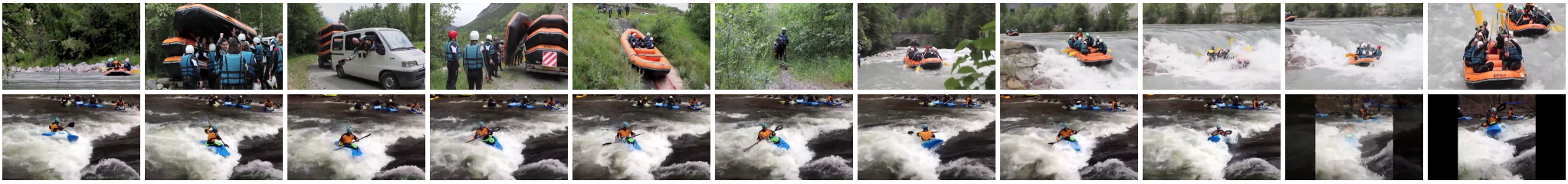
(a)

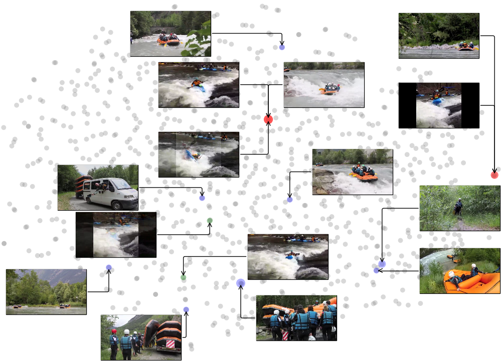
(b)

Figure 1: Examples of visual similarities. (a) Two video fragments with about 28 seconds from YouTube (v dBNZf90PLJ0 and v j3QSVh AhDc). They share some visual similar short clips. (b) A 2D t-SNE representation for the whole visual vocabulary. Some shared fragments are highlighted in red.

Based on this capability and also on the fact that the audio content of a video does not always match its visual content, in this work we propose a method to extract visual similarity information between short clips (i.e., videos up to $2.56$ seconds) grouped without human supervision, showing how to perform dense video captioning using this descriptor and deep visual features.

The idea behind the proposed method is that long and complex events can be decomposed into short and simple events, as illustrated in Figure LABEL:fig:similarityillustration_a – which shows two videos of related water sports: rafting and kayaking. We first identify similar events by splitting the videos into short clips and then extract visual features using the i3D method [3] for each short clip. A mini-batch $k$-means method groups representations based on their Euclidean distance producing a visual codebook, and a discrete representation is obtained by the sequence of cluster label numbers. Afterward, inspired by the GloVe method [23], we compute a co-occurrence matrix for this codebook and learn a dense representation by training a neural network to predict the pre-computed co-occurrence probability of any two visual words, as detailed in Section 3.1.

In Figure LABEL:fig:similarityillustration_b, a 2D t-SNE [19] visualization was used to project the entire visual codebook (drawn as gray dots). The clips from the first and second videos are represented with blue and green dots, respectively. Observe that the final content from the first video is much similar to the content of the second one (see the red dots) and that fragments with similar content are close to each other.

Our semantic descriptor can be easily adopted for the dense video captioning task proposed by Krishna et al. [14], which consists of two subtasks: temporal event proposal and video captioning. In this work, we employ a popular strategy of handling these tasks independently. More specifically, we use a multi-headed bi-modal proposal module [11] for event proposal generation, and a vanilla transformer [29] for video captioning.

In summary, the contributions of this work are: (i) we propose an unsupervised descriptor that can be easily employed in video understanding tasks; (ii) the visual similarity proved to be efficient to generate event proposals replacing the audio signal adopted in [11]; and (iii) our captioning results in the more complex scenario (i.e., learned proposals) show that the descriptor was able to adequately capture the visual similarity between seen and unseen clips, achieving state-of-the-art performance considering only visual features and competitive performance compared to multi-modal methods.

2 Related work

Dense video captioning was introduced in [14] and refers to proposing a temporal event localization in untrimmed videos (i.e., event proposal generation) and providing a suitable description for the event in fluent natural language (i.e., video captioning).

2.1 Event proposal generation

Event proposal generation is a challenging task because events have no predefined length, ranging from short frame sequences to very long frame sequences with partial or complete overlap. The general strategy is to define a set of anchors and a deep representation that encodes the video. Each anchor receives a confidence score from binary classifiers, and the highest-scoring anchors are passed to the captioning module jointly with their associated representation.

Krishna et al. [14], for example, used a forward sliding window strategy, based on Deep Action Proposals (DAPs) [7], with four strides ($1$, $2$, $4$, $8$), to sample video features with different time resolutions and feed them into a Long Short-Term Memory (LSTM) unit that encodes and provides past and current contextual information. On the other hand, Wang et al. [33] proposed to explore not only past and current context but also the future context to predict and estimate confidence scores. They adopted a forward and a backward pass on the LSTM units and merged the confidence scores using a multiplicative strategy. They also proposed an attentive fusion approach to compute the hidden representation. In both works, there are two models, one for each task, trained with an alternate procedure where the proposal module is trained first and then the captioning module is trained while the proposals are fine-tuned.

While most works overlooked the intrinsic relationship between the linguistic description and the visual appearance of the events, taking into account only visual features obtained by the C3D model [27] pre-trained on the Sports 1-M dataset [12], Zhou et al. [38] leveraged the influence of the linguistic description in the proposal module with a vanilla transformer model trained in an end-to-end manner. Similarly, Iashin and Rahtu [11] proposed a Bi-Modal Transformer (BMT) model using i3D [3] and VGGish [10] features (i.e., visual and audio) to learn video representations conditioned by their linguistic description. First, the authors trained a captioning model using the ground truth events and sentences. Then, they used the encoder to feed a multi-headed event proposal module composed of 1D Convolutional Neural Networks (CNNs) with different kernel sizes.

2.2 Video captioning

Considering the captioning task, most recent methods address this problem in two steps [31, 32, 5]. In the first step, a neural network encodes the entire video, frame by frame, into a compressed representation given by the hidden state of a Recurrent Neural Network (RNN). Then, in the second step, a decoder, usually an RNN, is fed with this representation to learn a probability distribution on a predefined vocabulary, producing a sentence, word-by-word. More recently, encoder-decoder models based on transformers [29] have been proposed [38, 15, 11], however, the best strategy for encoding video information before feeding the encoder remains an open issue. On the one hand, 2D CNN models can be fed frame by frame, producing long-range feature sequences that are difficult to process using RNN due to the well-known vanishing and exploding gradient problems [16]. LSTM and Gated Recurrent Unit (GRU) combined with soft and hard attention, or even Transformers with self-attention mechanisms, conduct the models to focus on more representative segments. These approaches boost performance but do not solve the video representation problem. On the other hand, when the entire video is fed into a 3D CNN (e.g., as in [37]), we come across the problem of information compression. All semantics are stored in a feature map with a fixed length, and converting this feature map in sentences is difficult because much relevant information can be lost or suppressed – especially on videos much longer than those used to train the 3D CNN.

This problem is more pronounced in captioning than in event proposal generation and has been circumvented by adding modalities such as audio and speech, objects, and action recognition [21, 8, 15, 11, 4]. For example, Iashin and Rahtu [15] proposed a framework called Multi-modal Dense Video Captioning (MDVC), in which each modality is fed into a separated encoder-decoder transformer and, in the end, their hidden representations are concatenated and fed to a language generator module composed of two dense layers and one softmax layer.

Chadha et al. [4] proposed a method to incorporate common-sense reasoning into the MDVC method. More specifically, they adapted common-sense reasoning from images [34] to videos, thus reaching impressive results in captioning – especially for the ground truth case. Although their proposal module uses the new feature to improve the bidirectional single-stream (Bi-SST) proposal generation method [33], we demonstrate that captioning results can be largely improved by replacing the proposal generation.

As mentioned earlier, state-of-the-art methods take advantage of multi-modal learning. However, it is difficult to provide more modalities for these models for three main reasons: (i) the models will be prone to overfitting due to their increased capacity; (ii) different modalities overfit and generalize at different rates, which requires multiple optimization strategies [35]; and (iii) more preprocessing is required to produce the features. Therefore, we provide a relevant contribution by extracting more video information using only visual features without any human annotations. Our method is an improved bag-of-words approach that is widely used in computer vision. However, to the best of our knowledge, it has not yet been applied to dense video captioning. Additionally, this type of information (i.e., co-occurrence similarity) is not easily learned by deep learning techniques, especially in an unsupervised manner, justifying our choice for the combination of k-means and global vectors. Finally, our descriptor can be concatenated with visual features, similarly to [4], for captioning and can replace the audio in the temporal proposal generation.

3 Methodology

In this work, we propose a dense video captioning system that leverages unsupervised semantic information and is trained in two steps. In the first step, a temporal event proposal module is responsible for generating central points, event lengths, and confidence scores, predicting whether an event is contained in that location. This proposal generator is trained adopting the architecture and procedures from Iashin and Rahtu [11], which are described in this section. Nevertheless, we replace the audio signal with the proposed semantic descriptor. Figure 2 shows the main elements of this step: a bi-modal transformer, a proposal generator, and a language generator.

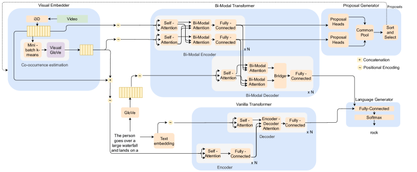
Figure 2: Overview of the proposed method. In the first stage, a bi-modal transformer is fed with visual and semantic co-occurrence-based features in a captioning task to learn the encoder parameters conditioned by language. Then, in the second stage, these parameters are used to predict temporal event proposals, Finally, these proposals are used to predict captions using a vanilla transformer and a language generator trained with ground-truth events and sentences.

In the second step, we employ the vanilla transformer used by Iashin and Rahtu [15], replacing the Bi-SST proposal module with the Bi-Modal Transformer (BMT) proposal module due to their state-of-the-art performance in event proposal generation. The main elements in this step are a vanilla transformer and a language generator. In both of them, we employ the proposed semantic descriptor, shown in Figure 2, for the element co-occurrence estimation.

Bi-modal and vanilla transformers are composed of encoder and decoder layers. As vanilla is the base for the construction of bi-modal, we first explain how the captioning module works and then how the proposal generator works.

3.1 Co-occurrence similarity estimation module

Let $D_{Tr}=\{V_{Tr_{1}},...,V_{Tr|D_{Tr}|}\}$ and $D_{Te}=\{V_{Te_{1}},...,V_{Te|D_{Te}|}\}$ be the training and testing datasets, respectively, composed of videos with long duration (e.g., $1$-$2$ min) and with more than one event per video. We first take all videos from $D_{Tr}$ and split each one into short clips with $f$ frames each. Then, we sample all these short clips and extract features using the i3D model [3]. As result, a set of features $X=\{x_{1},x_{2},...,x_{l}\}$, where $l=\lfloor n_{f}/f\rfloor$ and $n_{f}$ is the number of frames of a given video, with $x\in\mathbb{R}^{1024}$ is produced per video. Next, a mini-batch $k$-means algorithm [25] is trained to minimize the Euclidean distance

$$\min{\sum_{x\in X}||Ecd(C,x)-x||^{2}}\,,$$ (1)

where $Ecd(C,x)$ stands for the nearest cluster center $c\in C$ to $x$ and $|C|$ corresponds to our codebook size (e.g., $1{,}500$ clusters).

Once we have trained the clustering model, a video can be processed by first splitting it into clips of $f$ frames and then extracting the i3D features (only RGB stream) from these clips assigning each one of them to a cluster. These sequences of labeled clusters build a storytelling, and we can learn information about their co-occurrence properties, similarly to the dense representation from the GloVe method [23].

We compute a matrix of co-occurrence counts, denoted by $Z$, whose entries $Z_{ij}$ tabulate the number of times the cluster $j$ occurs in the context $S$ (an arbitrary sliding window) of cluster $i$.

Let $Z_{i}=\sum_{k}Z_{ik}$ be the number of times any cluster appears in the context of cluster $i$, we define the co-occurrence probability as

$$P_{ij}=P(j|i)=\frac{Z_{ij}}{Z_{i}}.$$ (2)

Pennington et al. [23] showed that the vector learning should be with ratios of co-occurrence probabilities rather than with the probabilities themselves, as this choice forces a greater difference in values between clusters that occur close frequently compared to infrequent cases. This ratio can be computed considering three clusters $i$, $j$ and $k$ with ($P_{ik}/P_{jk}$) and the model takes the general form given by

$$F(w_{i},w_{j},\tilde{w}_{k})=\frac{P_{ik}}{P_{jk}}\,,$$ (3)

where $w\in\mathbb{R}^{128}$ are cluster vectors and $\tilde{w}\in\mathbb{R}^{128}$ are separate context cluster vectors. Our model is a weighted least square regression trained with a cost function given by

$$J=f(Z_{ij})\sum_{i,j=1}^{|C|}{(w_{i}^{T}\tilde{w}_{j}+b_{i}+\tilde{b}_{j}-\log{Z_{ij}})^{2}}\,,$$ (4)

where $|C|$ is the size of the vocabulary (i.e., $1{,}000$ clusters), $b_{i}$ and $\tilde{b}_{j}$ are bias vectors and $f$ is a weighted function defined as

$$f(t)=\left\{\begin{array}[]{ll}(t/t_{\max})^{\alpha}&\mbox{if }t<t_{\max}\\ 1&\mbox{otherwise }\end{array}\right.,$$ (5)

where $t_{\max}=100$ and $\alpha=3/4$. More details and a complete mathematical description are provided in [23]. For our purposes, we adopt $w$ as our semantic descriptor, represented as Sm in the remainder of this work.

3.2 Video captioning module

Given a video $V$, the video captioning module takes a set of $n_{c}$ visual features $V_{f}=\{v_{f_{1}},...,v_{f_{n_{c}}}\}$, one per each clip, and a set of $m$ words $Y=\{y_{1},...,y_{m}\}$ to estimate the conditional probability of an output sequence given an input sequence.

We encode $v_{f_{c}}$, where $1\leq c\leq n_{c}$ as a concatenation of features defined as

$$v_{f_{c}}=[V_{E}(v_{c}),\textit{Sm}(v_{c})]\,,$$ (6)

where $V_{E}(\cdot)$ yields a deep representation given by an off-the-shelf neural network (e.g., i3D [3] with RGB or RGB + Optical Flow (OF) streams), $\textit{Sm}(\cdot)$ produces our co-occurrence similarity representation (see Section 3.1), $[\text{ }]$ is a concatenation operator, and $v_{c}$ is the $c$-th short clip for the video $V$.

The video features are fed to the original transformer model [29], composed of several layers (as shown in Figure 2), in which an encoder maps a sequence of visual features to a continuous representation that is used by a decoder to generate a sequence of symbols $Y$.

First, the visual embedding of each video is computed using Equation 6 and feeds all at once. Then, to provide information on the position of each feature we employ the same encoding method used by Vaswani et al. [29], a position-wise layer computes the position with sine and cosine at different frequencies as follows

$$\textit{PE}_{(pos,2i)} = \sin{(pos/10000^{2i/d_{model}})},$$ (7)

$$\textit{PE}_{(pos,2i+1)} = \cos{(pos/10000^{2i/d_{model}})},$$

where $pos$ is the position of the visual feature in the input sequence, $0\leq i<d_{model}$ and $d_{model}$ is a parameter defining the internal embedding dimension in the transformer.

In the encoder, these representations are passed through a multi-head attention layer. The attention used is the scaled dot-product and is defined in terms of queries ($\mathbf{Q}$), keys ($\mathbf{K}$), and values ($\mathbf{V}$) as

$$\textit{Att}(\mathbf{Q},\mathbf{K},\mathbf{V})=\textit{softmax}(\frac{\mathbf{Q}\mathbf{K}^{T}}{\sqrt{d_{k}}}).$$ (8)

The multi-head attention layer is defined by the concatenation of several heads ($1$ to $h$) of attention applied to the input projections as

$$\textit{MHAtt}(\mathbf{Q},\mathbf{K},\mathbf{V})=[head_{1},...,head_{h}]W^{0}\,,$$ (9)

where $\textit{head}_{i}=\textit{Att}(\mathbf{Q}W_{i}^{\mathbf{Q}},\mathbf{K}W_{i}^{K},\mathbf{V}W_{i}^{\mathbf{V}})$ and $[\text{ }]$ is a concatenation operator.

Once we compute self-attention, $\mathbf{Q}=\mathbf{K}=\mathbf{V}=V_{f}^{\textit{PE}}$, which results in

$$\begin{split}V_{f}^{self-att}=[\textit{Att}(V_{f}^{\textit{PE}}W_{i}^{V_{f}^{\textit{PE}}},V_{f}^{\textit{PE}}W_{i}^{V_{f}^{\textit{PE}}},V_{f}^{\textit{PE}}W_{i}^{V_{f}^{\textit{PE}}}),\\ ...,\textit{Att}(V_{f}^{\textit{PE}}W_{h}^{V_{f}^{\textit{PE}}},V_{f}^{\textit{PE}}W_{h}^{V_{f}^{\textit{PE}}},V_{f}^{\textit{PE}}W_{h}^{V_{f}^{\textit{PE}}})].\end{split}$$ (10)

At the end of each encoder layer, a fully connected feed-forward network $\textit{FFN}(\cdot)$ is applied to each position separately and identically. It consists of two linear transformations with a ReLU activation and is defined as

$$\begin{split}\textit{FFN}(u)=\max(0,uW_{1}+b_{1})W_{2}+b_{2}\end{split}\;,$$ (11)

resulting in $V_{f}^{\textit{FFN}}$ that is used in the decoder layer.

The decoder layer receives words and feeds an embedding layer $\textit{E}(\cdot)$, computing a position with Equation 7 resulting in $W^{\textit{PE}}$. Then, this representation is fed to the multi-head self-attention layer (see Equation 9), resulting in $W^{self-att}$. At this moment, the visual encoding provided by encoder layers feeds a multi-head attention layer as

$$W^{VisAtt}=\textit{MHAtt}(W^{self-att},V_{f}^{\textit{FFN}},V_{f}^{\textit{FFN}}).$$ (12)

Finally, $W^{VisAtt}$ feeds an $\textit{FFN}(\cdot)$ and, then, a generator $G(\cdot)$ composed of a fully connected layer and a softmax layer is responsible for learning the predictions over the vocabulary distribution probability.

3.3 Event proposal module

The event proposal module uses the bi-modal transformer. Considering the encoder, this transformer has two differences from the vanilla encoder. It takes two streams, visual $V_{f}$ and semantic Sm, separately, and it has three sub-layers in the encoder: self-attention (Equation 8), producing $V_{f}^{self-att}$ and $\textit{Sm}^{self-att}$; bi-modal attention, i.e.,

$$V_{f}^{\textit{Sm}-att} = \textit{MHAtt}(V_{f}^{self},\textit{Sm}^{self},\textit{Sm}^{self}),$$ (13)

$$\textit{Sm}^{Vis-att} = \textit{MHAtt}(\textit{Sm}^{self},V_{f}^{self},V_{f}^{self}),$$ (14)

and a fully connected layer $\textit{FFN}(\cdot)$ for each modality attention, producing $V_{{\textit{Sm}-att}}^{\textit{FNN}}$ and $\textit{Sm}_{v-att}^{\textit{FNN}}$ used in the bi-modal attention unit on the decoder and in the multi-headed proposal generator.

In the bi-modal decoder, the differences to the vanilla decoder are the bi-modal attention and bridge layers. First, a $W^{self-att}$ is obtained with Equation 9. Afterward, the bi-modal attention is computed as

$$W^{\textit{Sm}-att}=\textit{MHAtt}(W^{self-att},\textit{Sm}_{v-att}^{\textit{FNN}},\textit{Sm}_{v-att}^{\textit{FNN}})\,,$$ (15)

and

$$W^{V-att}=\textit{MHAtt}(W^{self-att},V_{{\textit{Sm}-att}}^{\textit{FNN}},V_{{\textit{Sm}-att}}^{\textit{FNN}}).$$ (16)

The bridge is a fully connected layer on the concatenated output of bi-modal attentions given as

$$W^{\text{FFN}}=\text{FFN}([W^{\textit{Sm}-att},W^{V-att}]).$$ (17)

The output of the bridge is passed through another FFN and then to the generator $G(\cdot)$. This means that the encoder parameters are learned in the captioning task, improving the visual features by conditioning them to the vocabulary.

More specifically, we focus on the $\textit{Sm}_{v-att}^{\textit{FNN}}$ and $V_{{\textit{Sm}-att}}^{\textit{FNN}}$ outputs. The proposal heads take these embeddings and make predictions for each modality individually, forming a pool of cross-modal predictions. The process begins with defining a $\Psi$ set of anchors with a central location and a prior length. A fully connected model with three 1D convolutional layers (with kernels $k_{1}=\text{arbitrary}$, $k_{2}=k_{3}=1$) predicts the value for the length and confidence score for each anchor. Then, these predictions are grouped and sorted by their confidences, preserving the proportionality between the source modalities. The process of selecting a $\Psi$ set of anchors follows the common approach of learning a $k$-means clustering model by grouping similar lengths using the ground-truth annotations [14, 33, 15, 4].

3.4 Training procedure

The first stage is the training of the semantic descriptor. We split each video from the training set into clips with $f=64$ frames and compute the i3D representation with only the RGB stream for each clip. Then, a mini-batch k-means learns a codebook with $|C|=1500$ visual words in a procedure with 5 epochs. Once we have learned the clustering model, the semantic embedding is trained using a sliding window $S=5$, corresponding to $\approx 10$ seconds and cluster embedding vectors with 128 dimensions. The training occurs up to 1500 iterations with an early stopping of 100 iterations. The Adagrad optimizer [6] with learning rate $lr=0.05$ is used.

The second stage is the training of the bi-modal encoder conditioned by the vocabulary. Thus, a captioning model is learned, using teaching forcing in which the target word is used as next input, instead of the predicted word, optimizing the KL-divergence loss, applying Label Smoothing [26] to make the model less confident over frequent words, and applying masking to prevent the model from attending on the next positions on the ground-truth sentences.

The model is learned up to 60 epochs with early stopping to monitor the METEOR score [2], using the Adam optimizer [13] with $\beta_{1}=0.9$, $\beta_{2}=0.999$, $lr=5.10^{-5}$ and $\epsilon=1.10^{-8}$. These procedures are also adopted in the final captioning training (i.e., using the vanilla transformer).

Finally, the bi-modal encoder is used to learn the multi-head proposal module with Mean Squared Error (MSE) for localization losses and cross-entropy for confidence losses. Then, we learn the final captioning model feeding the vanilla transformer [29] with ground-truth proposals and sentences. Thus, we predict the sentences to evaluate the performance.

4 Dataset and evaluation metrics

All experiments were performed on the ActivityNet Captions dataset [14], which is a large-scale dataset with temporal segments annotated and described in the proportion of one sentence for each segment. ActivityNet Captions contains $20{,}000$ videos divided into training/validation/test subsets with $50$/$25$/$25$% videos respectively and $3.65$ events per video on average. As the annotations of the test set are not public, we used the validation set for testing, as in previous works [33, 4, 15, 11].

The validation set was annotated twice (val1 and val2), and we consider the average for each evaluation metric on each validation split. The captioning task was evaluated using the BLEU@1-4 [22], METEOR [2], ROUGE_L [18] and CIDEr-D [30] metrics computed with the evaluation script provided by Krishna et al. [14], whereas event proposal was evaluated with Precision, Recall and F1-score (i.e., the harmonic mean of precision and recall).

5 Results

This section discusses our results on event proposal generation and video captioning using only visual features. We present a comparison with state-of-the-art (SOTA) methods and qualitative analysis.

As described in Section 3.4, we explored the captioning training to learn the parameters of the bi-modal encoder and then used this encoder to predict the proposals in the bi-modal proposal generator module. Afterward, these proposals were employed in a vanilla transformer captioning model.

Table 1 shows the BMT performance on video captioning. We highlighted as baselines the results from Iashin and Rahtu [11] with only visual features (i.e., using a vanilla transformer) and with bi-modal features (i.e., using visual and audio features denoted by BMT). Additionally, we included the performance from Iashin and Rahtu [15] with visual, audio, and speech modalities and employing Bi-SST as the event proposal module. Lastly, we investigated how BMT captioning performs with RGB+Sm and with V+Sm (i.e., RGB+OptFlow  +  Sm).

Table 1: Captioning performance comparison of BMT and Transformer methods with different features in the same validation sets. For each metric, the top $2$ results are highlighted in bold.

	GT Proposals			Learned Proposals
	B@3	B@4	M	B@3	B@4	M
Visual [11]	3.77	1.66	10.29	2.85	1.30	7.47
BMT [11]	4.62	1.99	10.89	3.84	1.88	8.44
MDVC${}_{\textit{Bi-SST}}$	4.52	1.98	11.07	2.53	1.01	7.46
BMT${}_{\textit{RGB+Sm}}$	4.12	1.72	10.32	3.62	1.74	8.03
BMT${}_{\textit{V+Sm}}$	4.32	1.85	10.55	3.68	1.81	8.26

Our results with V+Sm presented superior performance compared to the Visual performance from [11] considering all metrics and proposals schemes (GT and learned). Comparing BMT with $\text{BMT}_{\textit{V+Sm}}$, we observed a slightly lower performance using Sm instead A (audio) considering all scores.

However, the proposed model was still capable of learning a high-quality encoder, as evidenced by the performances achieved on proposal generation (see Table 2). We reached competitive results in terms of F1-score and Precision compared to the original BMT in the V+Sm scenario. This slight difference in F1-score supports the adoption of only visual features for event proposal generation due to the fewer preprocessing requirements than BMT. Considering the performance on RGB+Sm configuration (i.e., even less preprocessing), we outperformed the popular Bi-SST method while achieving competitive performance with BMT. Masked transformer [38], which is a method that explores only visual features and linguistic information to learn temporal proposals, is outperformed by our approach in $11.8$% [i.e., 59.60/53.31] in terms of F1-score.

Table 2: Comparison with state-of-the-art proposal generation. Results are reported on the validation sets using Precision, Recall and F1-score and are taken for $100$ proposals per video ratio. For each metric, the top $2$ results are highlighted in bold.

	FD	Prec.	Rec.	F1
MFT [36]	✓	51.41	24.31	33.01
BiSST [33]	✓	44.80	57.60	50.40
Masked Transf. [38]	✓	38.57	86.33	53.31
SDVC [20]	✓	57.57	55.58	56.56
BMT [11]	✗	48.23	80.31	60.27
OursRGB+Sm	✗	47.27	78.71	59.07
OursV+Sm	✗	48.11	78.31	59.60

Table 3: Results on the ActivityNet Captions dataset [14] adopting the MDVC method and the same validation sets used in iPerceive [4]. V = i3D output for RGB and Optical Flow (OF) streams; A = audio; S = speech; Sm = co-occurrence similarity; B = BLEU@N; M = METEOR; R = Rouge_l; and C = CIDEr-D. For each metric, the top $2$ results are highlighted in bold.

#	$V$		$A$	$S$	$Sm$	GT Proposals					Learned Proposals
	RGB	OF				B@3	B@4	M	R	C	B@3	B@4	M	R	C
1	✓	✓				5.40	2.67	11.18	22.90	44.49	4.40	2.46	8.58	13.36	13.03
2	✓	✓	✓			5.67	2.75	11.37	23.69	46.19	4.49	2.50	8.62	13.49	13.48
3	✓	✓	✓	✓		5.61	2.69	11.49	23.82	46.29	4.41	2.31	8.50	13.47	13.09
4	✓				✓	5.40	2.55	11.06	23.01	42.53	4.37	2.42	8.52	13.40	12.14
5	✓	✓			✓	5.54	2.64	11.23	23.34	45.76	4.57	2.55	8.65	13.62	12.82

Motivated by the event proposal performance, we adopt the same features and validation sets from BMT in both our method and MDVC baseline. This enables a fair comparison with MDVC and iPerceive [4] SOTA methods, as there are a few differences between the filtered validation sets used to evaluate BMT and MDVC. There are also differences in the number of frames used to extract visual features with the i3D method ($24$ frames [15] $\times$ $64$ frames in our experiments).

Table 3 shows the results of MDVC with the same features as BMT and with our temporal proposals using V (#1), V+A (#2) and V+A+S (#3), where V = i3D output for RGB and OF streams, A = audio, and S = speech. Considering the most challenging scenario, learned proposals, V+A presented better results than V+A+S and our results V+Sm were the best in the METEOR and BLEU scores. It can be noted that audio and speech had a greater impact on the ground truth proposals than in learned proposals results. Finally, our performance with RGB+Sm in learned proposals is competitive with the multi-modal approach.

In Table 4, we show a comparison between our results and those obtained by SOTA methods. As can be seen, there are methods based only on visual features and methods based on multi-modal features (see column VF). As the videos from ActivityNet captions must be downloaded from YouTube, several videos have become unavailable since the original dataset was published. Hence, we used $91$% of the dataset (this information is presented in column FD, where a “✓” means that $100$% of the videos were available at the time of the experiments). As we have a reduced set of videos for evaluation, the validation sets were filtered to contain only the videos downloaded. As demonstrated in [11], this procedure enables a fair comparison because the SOTA methods reached almost unchanged results when evaluated using these filtered validation sets. However, do not consider this procedure is unfair because the model is forced to propose events and generate captions for unseen videos, reducing performance. Finally, some works adopted a direct optimization of the METEOR score with reinforcement learning techniques (see column RL). We also listed the performance without these techniques since, as shown in Table 4 for DVC [17], these techniques boosted the METEOR score without a proportional boost in BLEU, which may not corresponds to an actual improvement in the captioning quality.

Table 4: Comparison with other methods on ActivityNet Captions (validation set). VF = Use only visual features; RL = Reinforcement Learning – reward maximization (METEOR); FD = Full dataset was available. The top $2$ results are highlighted in bold.

	VF	RL	FD	GT Proposals			Learned Proposals
				B@3	B@4	M	B@3	B@4	M
DVC [17]	✓	✓	✓	4.55	1.62	10.33	2.27	0.73	6.93
SDVC [20]	✓	✓	✓	4.41	1.28	13.07	2.94	0.93	8.82
Dense Cap [14]	✓	✗	✓	4.09	1.60	08.88	1.90	0.71	5.69
DVC [17]	✓	✗	✓	4.51	1.71	09.31	2.05	0.74	6.14
Masked Transf. [38]	✓	✗	✓	5.76	2.71	11.16	2.91	1.44	6.91
Bi-SST [33]	✓	✗	✓	$-$	$-$	10.89	2.27	1.13	6.10
SDVC [20]	✓	✗	✓	$-$	$-$	$-$	$-$	$-$	6.92
MMWS [24]	✗	✗	✗	3.04	1.46	07.23	1.85	0.90	4.93
BMT [11]	✗	✗	✗	4.63	1.99	10.90	3.84	1.88	8.44
iPerceive [4]	✗	✗	✗	6.13	2.98	12.27	2.93	1.29	7.87
MDVC [15]	✗	✗	✗	5.83	2.86	11.72	2.60	1.07	7.31
TSP [1]	✗	✗	✗	$-$	$-$	$-$	4.16	2.02	8.75
Ours${}_{\textit{RGB+Sm}}$	✓	✗	✗	5.40	2.55	11.06	4.37	2.42	8.52
Ours${}_{\textit{V+Sm}}$	✓	✗	✗	5.54	2.64	11.23	4.57	2.55	8.65

Considering only the single modality scenario, without RL, our model outperforms all other methods in learned proposals and has a slightly lower performance on BLEU@3-4 than the Masked Transformer for GT proposals. Compared to the multi-modal methods, our performance on ground truth is lower than the MDVC and iPerceive methods. However, we remark that the performance on GT proposals is an indicator of how good the captions are when the event is perfectly delimited. As can be seen in Table 2, we are far from this reality, and the most relevant performance to be taken into account is in the learned proposals scenario, where our results are remarkable.

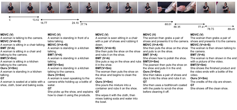
Figure 3: Qualitative comparison between MDVC, BMT and the proposed method using the video with id v_EFGtb9IDQao. We present the predictions from leaned proposals scenario. The results from BMT make use of the proposals learned with V+A, whereas MDVC and our method make use of the proposals learned with V+Sm due to their higher F1-score compared to the Bi-SST used in [15].

Finally, we highlight the results of the TSP method [1] compared to ours. This method includes an improved visual descriptor for temporal event localization that combines local features optimized by accuracy on trimmed action classification (TAC) and global features given by pooling local predictions. The authors employed the R(2+1)D architecture [28] fine-tuned on the ActivityNet v1.3 dataset [9]. They adopted the BMT model for captioning, and a critical procedure for the success of video captioning was the fine-tuning on ActivityNet with trimmed action annotations (METEOR of $8.75$ with fine-tuning and $8.42$ without [1]). Lastly, their model also considers the audio signal. Thus, it is noteworthy that our model reaches a comparable performance on METEOR without audio and action annotations.

In Figure 3, we show a qualitative analysis of dense captioning. We selected an instructional video that presents highly correlated visual and audio signals. A woman behind a table explains how to clean a shoe using a toothbrush, a cloth, and baking soda. This is a challenging scenario for our visual-based method, as there are not many visual changes that it can easily detect throughout the video. We chose the following methods for comparison: MDVC [15] with only visual and with visual, audio, and speech modalities; BMT [11] with visual and audio and with visual and semantic modalities; and finally, the proposed method.

Our method incorrectly identified that a woman is standing (and not sitting) in the video, but this is not easy to recognize even for humans. Then, it recognizes that the woman talks to the camera and that there is a bottle of water. Some methods, including ours, inferred that the woman is in a kitchen, but it is impossible to determine if they are correct. Only our method recognizes the act of mixing things on a container. We believe it focuses on the woman’s hands and associates this action with other cleaning videos. No method was able to identify the use of a toothbrush outside its usual context, and only the BMT (V+Sm) was able to predict the cleaning action, which is remarkable because it does not explore the audio signal – ignoring the woman’s explanation.

6 Conclusions and future work

In this work, we presented a method to enrich visual features for dense video captioning that learns visual similarities between clips from different videos and extracts information on their co-occurrence probabilities. Our conclusions are: (i) co-occurrence similarities combined with deep features can provide more meaningful semantic information for dense video captioning than only deep features from a single modality; (ii) our semantic features processed with an encoder-decoder scheme based on transformers outperformed single modality methods while achieving competitive results with multi-modal state-of-the-art methods; and (iii) we reached impressive results adopting only the RGB stream when compared to results using RGB, optical flow, and audio information.

As directions for future work, deep clustering methods could replace the mini-batch $k$-means. As our method is unsupervised, multiple large-scale visual datasets could be combined without the need for linguistic descriptions or human annotations. These datasets could be used to learn more accurate/detailed codebooks using co-occurrences or BERT-based models.

Appendix A Semantic Descriptor Evaluation

We evaluated the semantic descriptor for its performance on the BMT model replacing the audio signal and considering ground truth and captioning of event proposals, Figure 4(a) and (b), and for performance of event proposals (c). We changed the vocabulary size $|C|$ (100, 500, 1000, 1500, and 2000) and the context window S (10s, 30s, and 60s). The graphs show that the descriptor performance varies slightly depending on the configuration. In this work, we conducted experiments considering the configuration with 1500 visual words and 10s of context window, as it reached the higher Meteor score for ground truth (10.6) and for captioning of event proposals (8.3).

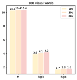
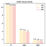
(a)

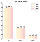
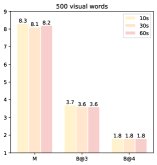
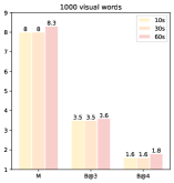
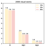
(b)

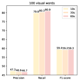
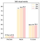
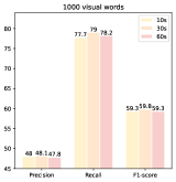
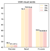
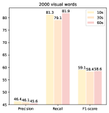
(c)

Figure 4: Captioning performances for ground truth and event proposals, (a) and (b), and for proposal generation (c) considering the BMT model replacing the audio signal with several semantic descriptors generated with different vocabularies (100, 500, 1000, 1500, 2000) and context windows (10s, 30s, 60s).

References

- Alwassel et al. [2020] Alwassel, H., Giancola, S., Ghanem, B., 2020. TSP: temporally-sensitive pretraining of video encoders for localization tasks. arXiv preprint arXiv:2011.11479, 1–18.
- Banerjee and Lavie [2005] Banerjee, S., Lavie, A., 2005. METEOR: An automatic metric for MT evaluation with improved correlation with human judgments, in: ACL Workshop on Intrinsic and Extrinsic Evaluation Measures for Machine Translation and/or Summarization, pp. 65–72.
- Carreira and Zisserman [2017] Carreira, J., Zisserman, A., 2017. Quo vadis, action recognition? a new model and the kinetics dataset, in: IEEE Conference on Computer Vision and Pattern Recognition (CVPR), pp. 4724–4733.
- Chadha et al. [2021] Chadha, A., Arora, G., Kaloty, N., 2021. iPerceive: Applying common-sense reasoning to multi-modal dense video captioning and video question answering. IEEE Winter Conference on Applications of Computer Vision (WACV) , 1–13.
- Donahue et al. [2015] Donahue, J., Anne Hendricks, L., Guadarrama, S., Rohrbach, M., Venugopalan, S., Saenko, K., Darrell, T., 2015. Long-term recurrent convolutional networks for visual recognition and description, in: IEEE Conference on Computer Vision and Pattern Recognition (CVPR), pp. 2625–2634.
- Duchi et al. [2011] Duchi, J., Hazan, E., Singer, Y., 2011. Adaptive subgradient methods for online learning and stochastic optimization. J. Mach. Learn. Res. 12, 2121–2159.
- Escorcia et al. [2016] Escorcia, V., Heilbron, F.C., Niebles, J.C., Ghanem, B., 2016. Daps: Deep action proposals for action understanding, in: European Conference on Computer Vision (ECCV), pp. 768–784.
- Gan et al. [2017] Gan, Z., Gan, C., He, X., Pu, Y., Tran, K., Gao, J., Carin, L., Deng, L., 2017. Semantic compositional networks for visual captioning, in: IEEE Conference on Computer Vision and Pattern Recognition (CVPR), pp. 1141–1150.
- Heilbron et al. [2015] Heilbron, F.C., Escorcia, V., Ghanem, B., Niebles, J.C., 2015. ActivityNet: A large-scale video benchmark for human activity understanding, in: IEEE Conference on Computer Vision and Pattern Recognition (CVPR), pp. 961–970.
- Hershey et al. [2017] Hershey, S., Chaudhuri, S., Ellis, D.P., Gemmeke, J.F., Jansen, A., Moore, R.C., Plakal, M., Platt, D., Saurous, R.A., Seybold, B., 2017. CNN architectures for large-scale audio classification, in: IEEE International Conference on Acoustics, Speech and Signal Processing (ICASSP), pp. 131–135.
- Iashin and Rahtu [2020] Iashin, V., Rahtu, E., 2020. A better use of audio-visual cues: Dense video captioning with bi-modal transformer, in: British Machine Vision Conference (BMVC), pp. 1–16.
- Karpathy et al. [2014] Karpathy, A., Toderici, G., Shetty, S., Leung, T., Sukthankar, R., Fei-Fei, L., 2014. Large-scale video classification with convolutional neural networks, in: IEEE Conference on Computer Vision and Pattern Recognition (CVPR), pp. 1725–1732.
- Kingma and Ba [2015] Kingma, D.P., Ba, J., 2015. Adam: A method for stochastic optimization, in: Bengio, Y., LeCun, Y. (Eds.), International Conference on Learning Representations (ICRL), pp. 1–15.
- Krishna et al. [2017] Krishna, R., Hata, K., Ren, F., Fei-Fei, L., Niebles, J.C., 2017. Dense-captioning events in videos, in: International Conference on Computer Vision (ICCV), pp. 706–715.
- lashin and Rahtu [2020] lashin, V., Rahtu, E., 2020. Multi-modal dense video captioning, in: IEEE/CVF Conference on Computer Vision and Pattern Recognition Workshops (CVPRW), pp. 4117–4126.
- Li et al. [2018] Li, S., Li, W., Cook, C., Zhu, C., Gao, Y., 2018. Independently recurrent neural network (IndRNN): Building a longer and deeper RNN, in: IEEE Conference on Computer Vision and Pattern Recognition (CVPR), pp. 5457–5466.
- Li et al. [2018] Li, Y., Yao, T., Pan, Y., Chao, H., Mei, T., 2018. Jointly localizing and describing events for dense video captioning, in: IEEE Conference on Computer Vision and Pattern Recognition (CVPR), pp. 7492–7500.
- Lin [2004] Lin, C., 2004. ROUGE: A package for automatic evaluation of summaries, in: Text Summarization Branches Out, Association for Computational Linguistics, Barcelona, Spain. pp. 74–81.
- van der Maaten and Hinton [2008] van der Maaten, L., Hinton, G., 2008. Visualizing data using t-SNE. Journal of Machine Learning Research 9, 2579–2605.
- Mun et al. [2019] Mun, J., Yang, L., Ren, Z., Xu, N., Han, B., 2019. Streamlined dense video captioning, in: IEEE Conference on Computer Vision and Pattern Recognition (CVPR), pp. 6588–6597.
- Pan et al. [2017] Pan, Y., Yao, T., Li, H., Mei, T., 2017. Video captioning with transferred semantic attributes, in: IEEE Conference on Computer Vision and Pattern Recognition (CVPR), pp. 984–992.
- Papineni et al. [2002] Papineni, K., Roukos, S., Ward, T., Zhu, W., 2002. BLEU: a method for automatic evaluation of machine translation, in: Annual Meeting of the Association for Computational Linguistics (ACL), pp. 311–318.
- Pennington et al. [2014] Pennington, J., Socher, R., Manning, C.D., 2014. GloVe: Global vectors for word representation, in: Conference on Empirical Methods in Natural Language Processing (EMNLP), pp. 1532–1543.
- Rahman et al. [2019] Rahman, T., Xu, B., Sigal, L., 2019. Watch, listen and tell: Multi-modal weakly supervised dense event captioning, in: IEEE International Conference on Computer Vision (ICCV), pp. 8907–8916.
- Sculley [2010] Sculley, D., 2010. Web-scale -means clustering, in: International Conference on World Wide Web, p. 1177–1178.
- Szegedy et al. [2016] Szegedy, C., Vanhoucke, V., Ioffe, S., Shlens, J., Wojna, Z., 2016. Rethinking the inception architecture for computer vision, in: IEEE Conference on Computer Vision and Pattern Recognition (CVPR), pp. 2818–2826.
- Tran et al. [2015] Tran, D., Bourdev, L., Fergus, R., Torresani, L., Paluri, M., 2015. Learning spatiotemporal features with 3D convolutional networks, in: IEEE International Conference on Computer Vision (ICCV), pp. 4489–4497.
- Tran et al. [2018] Tran, D., Wang, H., Torresani, L., Ray, J., LeCun, Y., Paluri, M., 2018. A closer look at spatiotemporal convolutions for action recognition, in: IEEE Conference on Computer Vision and Pattern Recognition (CVPR), pp. 6450–6459.
- Vaswani et al. [2017] Vaswani, A., Shazeer, N., Parmar, N., Uszkoreit, J., Jones, L., Gomez, A.N., Kaiser, L., Polosukhin, I., 2017. Attention is all you need, in: International Conference on Neural Information Processing, pp. 6000–6010.
- Vedantam et al. [2015] Vedantam, R., Zitnick, C.L., Parikh, D., 2015. CIDEr: consensus-based image description evaluation, in: IEEE Conference on Computer Vision and Pattern Recognition (CVPR), pp. 4566–4575.
- Venugopalan et al. [2015] Venugopalan, S., Rohrbach, M., Donahue, J., Mooney, R., Darrell, T., Saenko, K., 2015. Sequence to sequence – video to text, in: IEEE International Conference on Computer Vision (ICCV), pp. 4534–4542.
- Venugopalan et al. [2015] Venugopalan, S., Xu, H., Donahue, J., Rohrbach, M., Mooney, R., Saenko, K., 2015. Translating videos to natural language using deep recurrent neural networks, in: Conference of the North American Chapter of the Association for Computational Linguistics – Human Language Technologies (NAACL HLT 2015), pp. 1494–1504.
- Wang et al. [2018] Wang, J., Jiang, W., Liu, W., Xu, Y., 2018. Bidirectional attentive fusion with context gating for dense video captioning, in: IEEE Conference on Computer Vision and Pattern Recognition (CVPR), pp. 7190–7198.
- Wang et al. [2020a] Wang, T., Huang, J., Zhang, H., Sun, Q., 2020a. Visual commonsense R-CNN, in: IEEE Conference on Computer Vision and Pattern Recognition (CVPR), pp. 10757–10767.
- Wang et al. [2020b] Wang, W., Tran, D., Feiszli, M., 2020b. What makes training multi-modal classification networks hard?, in: IEEE/CVF Conference on Computer Vision and Pattern Recognition (CVPR), pp. 12692–12702.
- Xiong et al. [2018] Xiong, Y., Dai, B., Lin, D., 2018. Move forward and tell: A progressive generator of video descriptions, in: European Conference on Computer Vision (ECCV), pp. 468–483.
- Xu et al. [2019] Xu, H., Li, B., Ramanishka, V., Sigal, L., Saenko, K., 2019. Joint event detection and description in continuous video streams, in: IEEE Winter Applications of Computer Vision Workshops (WACV), pp. 25–26.
- Zhou et al. [2018] Zhou, L., Zhou, Y., Corso, J.J., Socher, R., Xiong, C., 2018. End-to-end dense video captioning with masked transformer, in: IEEE/CVF Conference on Computer Vision and Pattern Recognition, pp. 8739–8748.