Contact simulation of a 2D Bipedal Robot kicking a ball

Abstract

This report describes an approach for simulating multi-body contacts of actively-controlled systems. In this work, we focus on the controls and contact simulation of a 2-dimensional bipedal robot kicking a circular ball. The Julia code and more video results of the contact simulation can be found at this URL: https://github.com/adubredu/contact_sim.jl

Figure 1: Biped robot walks to towards the ball and kicks it.

I Introduction

I-A Motivation and Context

Contact resolution is useful for actively-controlled rigid-body systems that make and break contact with their environment. The ability to resolve contact forces after collision with a rigid body enables the prediction of the system’s motion after impact. The resolved contact forces can then be accounted for in the system’s feedback controllers in order to keep the system stable and functional.

I-B Problem Statement

In this project, we simulate multi-body contacts of an actively-controlled rigid-body system. More specifically, we focus on the contact simulation and control of a 2-dimensional bipedal robot kicking a circular ball. We assume plastic contacts for the foot of the 2D bipedal robot as it walks on the flat ground and elastic contacts for the circular ball as it bounces on the ground after being kicked.

I-C Overview

The remaining sections are organized as follows; In Section III-A, we describe our general approach for contact resolution for rigid bodies. Next, in Sections III-B and III-C , we describe how we apply contact resolution for simulating contacts of a circular ball and a 2D bipedal robot respectively. Finally, we describe how we incorporate resolved contact forces in controlling the locomotion of the 2D bipedal robot. We provide qualitative and quantitative results in Section IV and conclude the report in Section VI

II Literature Review

Contact resolution has been studied extensively both in the field of robot manipulation [5, 10, 7] and robot locomotion [2, 3, 6]. This work aims to simulate contacts of an actively-controlled bipedal robot that interacts with a passive rigid body. We resolve contacts using the linear complementarity formulation as has been pursued in works like [8, 4].

III Methodology

III-A Linear Complementarity Formulation for Contact Resolution

Since most contact mechanics constraints have complementarity relationships, one common way of resolving contact forces after impact is to formulate contact resolution as a Linear Complementarity Problem (LCP). Linear Complementarity Problems have the form

$$\max_{z} z^{T}\cdot(V\cdot z+p)$$ (1)

s.t. $$V\cdot z+p\geq 0$$

$$z\geq 0$$

where $V\cdot z+p\geq 0$ and $z\geq 0$ have the complementarity relationship $V\cdot z+p\geq 0\leavevmode\nobreak\ \bot\leavevmode\nobreak\ z\geq 0$, which implies that, element-wise, at least one of the expressions on the other side of $\bot$ takes on a value of $0$.

To formulate contact mechanics constraints of a rigid body as an LCP, we first discretize the dynamics equation

$$M(q)\dot{v}+c(v,q)+g(q)=f_{e}$$ (2)

$$v=\dot{q}$$

by taking first-order zero-hold discrete-time approximation. We then rearrange the terms to express the equations in terms of the position and velocity of the body in the next time step as

$$v_{t+1}=v_{t}+\Delta tM^{-1}(q_{t})k(v_{t},q_{t})+f_{e,t}$$ (3)

$$q_{t+1}=q_{t}+\Delta tv_{t}$$

Finally, we introduce the reaction forces due to contact and their relevant constraints to form the system of equations and constraints

$$v_{t+1}=v_{t}+\Delta tM^{-1}(q_{t})(k(v_{t},q_{t})+f_{e,t}+J_{c}(q_{t})f_{c,t})$$ (4)

$$q_{t+1}=q_{t}+\Delta tv_{t}$$

$$\phi(q_{t})\geq 0\leavevmode\nobreak\ \bot\leavevmode\nobreak\ f_{n}\geq 0$$

$$f_{n}\geq 0\leavevmode\nobreak\ \bot\leavevmode\nobreak\ n^{T}(V_{t+1}+\epsilon v_{t})\geq 0$$

$$f_{t}\geq 0\leavevmode\nobreak\ \bot\leavevmode\nobreak\ \lambda e+D^{T}v_{t+1}\geq 0$$

$$\lambda\geq 0\leavevmode\nobreak\ \bot\leavevmode\nobreak\ \mu f_{n}-e^{T}f_{t}\geq 0$$

where $M$ is the mass-inertia matrix of the rigid body, $k(v_{t},q_{t})$ stands for the coriolis and conservative forces terms, $f_{e,t}$ and $f_{c,t}$ are the external and contact forces at time $t$ respectively, $J_{c}(q_{t})$ is the contact Jacobian, $q_{t}$ and $v_{t}$ are the position and velocity of the rigid body at time $t$, $\phi(q_{t})$ is the minimum distance to contact, $f_{n}$ and $f_{t}$ are the normal and tangential components of the contact force $f_{c}$, $\epsilon$ is the coefficient of restitution, $\lambda$ is a scalar that represents the relative tangential velocity term and $\mu$ is the coefficient of friction.

These equations are rearranged into the LCP form

$$V\cdot z+p\geq 0$$

where $V=$

$$\begin{bmatrix}\Delta t\cdot n^{T}M^{-1}n&\Delta t\cdot n^{T}M^{-1}D&0\\ \Delta t\cdot D^{T}M^{-1}n&\Delta t\cdot D^{T}M^{-1}D&e\\ \mu&-e^{T}&0\end{bmatrix}$$ (5)

$z=$

$$\begin{bmatrix}f_{n}\\ f_{t}\\ \lambda\end{bmatrix}$$ (6)

and $p=$

$$\begin{bmatrix}n^{T}((1+\epsilon)v_{t}+\Delta tM^{-1}(k+f_{e}))\\ D^{T}(v_{t}+\Delta tM^{-1}(k+f_{e}))\\ 0\end{bmatrix}$$ (7)

The solution of this Contact Resolution LCP returns the contact forces, $f_{n}$ and $f_{t}$, as well as the relative motion term $\lambda$.

To solve this LCP problem, we redefine it into a Quadratic Program and solve it using Ipopt [9], which is an off-the-shelf Nonlinear Program Solver that is capable of solving Quadratic Programs. Any off-the-shelf Quadratic Program solver could have been used in place of Ipopt.

The algorithm for contact simulation is summarized in Algorithm 1. At each time step, a collision checking routine checks for contact. If there is no contact, we simply run a forward simulation of the body’s dynamics. If there is contact, the LCP problem is formulated and solved. The solution contact forces are then used to predict the motion of the body in the next time step.

Algorithm 1 Contact Simulation

Data: Object Geometry, Object Inertial Properties, Friction, Restitution, Initial Conditions

Result: Object Trajectory

set initial values for $q$ and $v$

while $t\leq T$ do

     flag = check_collision($q_{t}$)

     if flag then

         $q_{t+1},v_{t+1}$ = solve_LCP($q_{t},v_{t}$)

     else

         $v_{t+1}=v_{t}+\Delta tM^{-1}(k_{t}+f_{c,t})$

         $q_{t+1}=q_{t}+\Delta tv_{t}$

     end if

     $t=t+1$

end while

III-B Contact resolution of the circular ball

To use the LCP formulation described in Section III-A, to perform contact resolution of the circular ball, all we had to do was to specify our configuration space and specify a function that computed both the contact Jacobian $J_{c}(q_{t})$ and minimum distance to contact $\phi(q_{t})$. Since the entire problem is in 2-D space, our body position $q$ and velocity $v$ are in SE(2) and are represented by $(x,y,\theta)$ and $(\dot{x},\dot{y},\dot{\theta})$ respectively. Given an initial position and velocity, the trajectory of the ball is simulated using Algorithm 1 above.

III-C Contact resolution of 2D Bipedal Robot

We approximate the foot of the 2D bipedal robot as a rectangle of specific width and length to simplify contact resolution. Just like in Section III-B, we represent the position and velocity of the foot in SE(2) space and specify a function for computing both the contact Jacobian and minimum distance to contact of the foot. Since the body of the 2D bipedal robot is made up of a torso and legs, both of which have mass, the mass-inertia matrix of the 2D bipedal robot, according to [1], is computed as $M=$

$$\begin{bmatrix}M_{11}&M_{12}&0\\ M_{21}&M_{22}&0\\ 0&0&I\\ \end{bmatrix}$$ (8)

where

$$M_{11}=2(I+m_{l}(c^{2}+l^{2}-cl-clcos(\theta)))+m_{t}l^{2}$$ (9)

$$M_{12}=I+m_{l}(c^{2}-clcos(\theta))$$

$$M_{21}=I+m_{l}(c^{2}-clcos(\theta))$$

$$M_{22}=I+c^{2}m$$

and $m_{l}$ is the mass of the leg, $c$ is the centroid of the leg, $l$ is the length of the leg, $m_{t}$ is the mass of the torso and $\theta$ is the angle between the legs.

III-D Control of 2D Bipedal Robot

The 2D bipedal robot has a single actuator situated at the hip that exerts a torque to swing the legs. As a result, the 2D bipedal robot is an underactuated system. We use partial feedback linearization to control the 2D biped robot as described below:

Given the dynamics equation of the 2D bipedal robot as

$$M\ddot{\theta}+N=B\cdot u$$ (10)

where $M$ is the mass-inertia matrix, $N$ is the sum of the coriolis and conservative forces terms, $B$ is the control selection matrix, $\theta=(\theta_{1},\theta_{2})$ are the 2 degrees of freedom of the robot and $u$ is the control input, we can rearrange the equation to make $\ddot{\theta}$ the subject of the equation as

$$\ddot{\theta}=M^{-1}\cdot(B\cdot u-N)$$ (11)

Since only the hip joint $\theta_{2}$ is actuated, we can describe the controlled joint $\theta_{c}$ as

$$\theta_{c}=S_{c}\cdot\theta$$ (12)

where $S_{c}$ is the selection matrix $[0;1]$. Taking the second derivative of Equation 12 gives us

$$\ddot{\theta_{c}}=S_{c}\cdot\ddot{\theta}=S_{c}\cdot M^{-1}\cdot(B\cdot u-N)$$ (13)

Using this trick now makes $\theta_{c}$ fully controllable. As such we can control $\theta_{c}$ to any reference value $\theta_{c}^{ref}$ using the PD controller

$$\ddot{\theta_{c}}=\ddot{\theta_{c}^{ref}}-K_{p}(\theta_{c}-\theta_{c}^{ref})-K_{d}(\dot{\theta_{c}}-\dot{\theta_{c}^{ref}})$$ (14)

Putting the expression for $\ddot{\theta_{c}}$ in Equation 14 back into Equation 13 and making the control input torque $u$ the subject, we get the expression of the control input torque as

$$u=(S_{c}\cdot M^{-1}\cdot B)^{-1}\cdot(\ddot{\theta_{c}}+S_{c}\cdot M^{-1}\cdot N)$$ (15)

III-E Kicking the ball

To kick the ball with a specified force $F_{k}$, we find the corresponding torque $\tau_{k}$ to be applied to the hip actuator of the 2D biped robot using

$$\tau_{k}=F_{k}\cdot l$$

where $l$ is the length of the leg. $\tau_{k}$ is then sent as a reference torque to the robot controller, which then computes the control input torque to set the hip actuator as described in Equations 10 - 15 above. Once the robot’s leg makes contact with the ball, the contact forces are resolved as described above and used to predict the velocity of the ball right after impact.

IV Experiments

We run the contact simulation of the 2D bipedal robot walking over to the circular ball and kicking it with varying torques. The ball had a mass of $0.04$kg and a diameter of $0.4$m. The robot had a torso mass of $1.0$kg, a leg mass of $0.5$kg and a leg length of $1.0$m. The kicking torques varied from $30$Nm to $100$Nm. The ball trajectories can be seen in the plots in Figure 2 below:

0pt

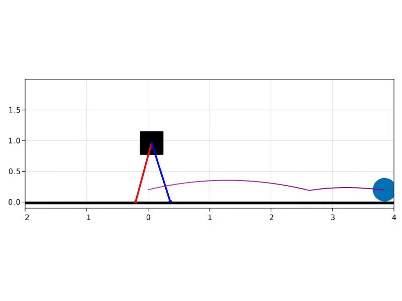
(a) 30Nm

(b)

0pt

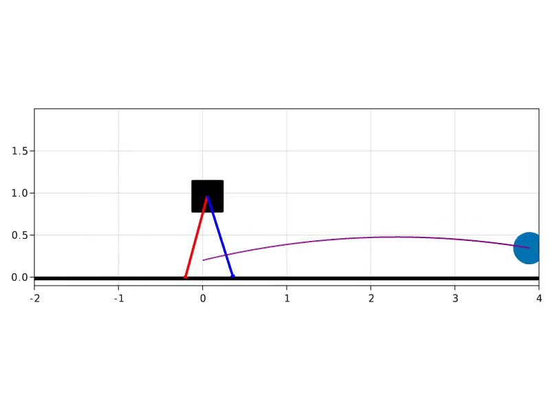
(c) 40Nm

(d)

0pt

(e) 50Nm

(f)

0pt

(g) 60Nm

(h)

0pt

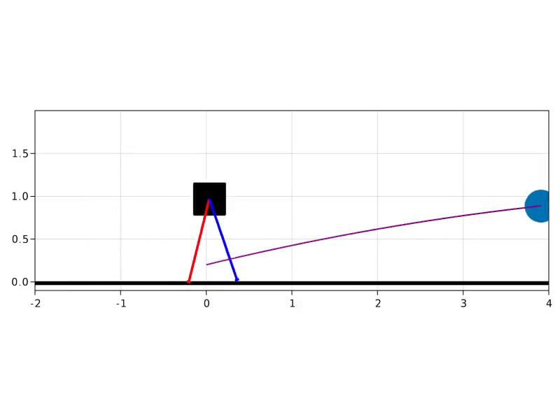
(i) 70Nm

(j)

0pt

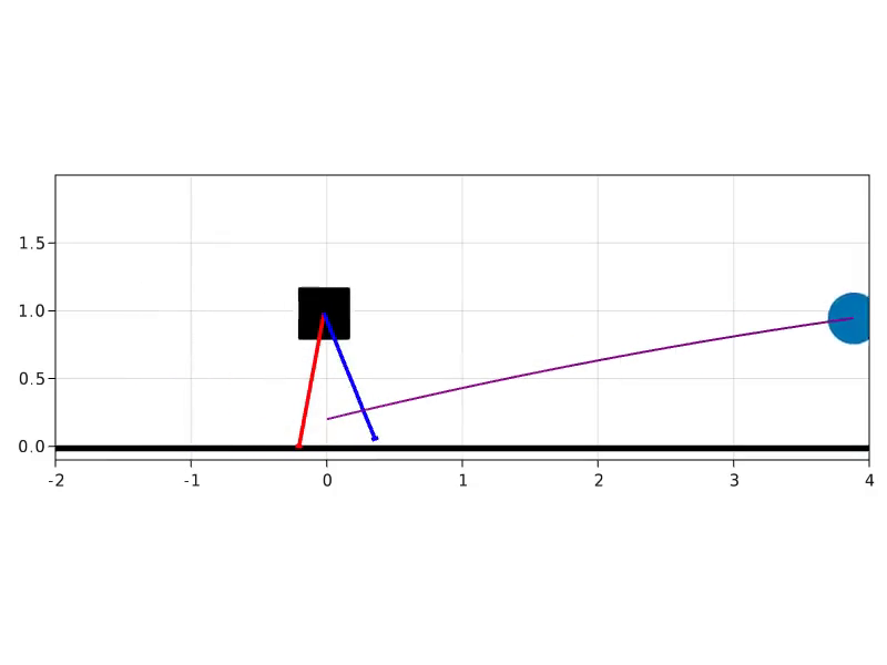
(k) 80Nm

(l)

0pt

(m) 90Nm

(n)

0pt

(o) 100Nm

(p)

Figure 2: Circular ball trajectories after being kicked by the 2D bipedal robot with torques from 30Nm to 100Nm

The ball velocities after being kicked with the various leg torques are presented in the table I below:

$\tau$ (N.m)	$v_{x}$ (m/s)	$v_{y}$ (m/s)
$30.0$	$7.29$	$1.78$
$40.0$	$9.71$	$2.38$
$50.0$	$12.14$	$2.97$
$60.0$	$14.57$	$3.57$
$70.0$	$17.00$	$4.16$
$80.0$	$19.43$	$4.75$
$90.0$	$21.86$	$5.35$
$100.0$	$24.28$	$5.94$

TABLE I: Ball velocities for varying kicking torques after kicking impact

V Discussion

The contact simulation of the 2D bipedal robot kicking the circular ball worked quite well. The main difficulty in this work was in implementing the partial feedback linearization controller for the bipedal robot’s locomotion. One potential improvement or extension to this work could be to simulate kicking contacts of more irregularly-shaped objects like bottles, buckets or even dogs!. Another extension of this work could be to simulate both arm and leg contacts of a dual-arm bipedal robot pushing a heavy cabinet through a doorway.

VI Conclusion

In this report, we described our approach for contact simulation of a 2D bipedal robot kicking a circular ball. We also provided experimental results for the different kicking torques. The code for this work and videos of the contact simulation can be found at this URL: https://github.com/adubredu/contact_sim.jl

References

- [1] Pranav Bhounsule. Legged robotics course. University of Illinois at Chicago, 2021.
- [2] Karim Bouyarmane and Abderrahmane Kheddar. Humanoid robot locomotion and manipulation step planning. Advanced Robotics, 26(10):1099–1126, 2012.
- [3] Justin Carpentier, Rohan Budhiraja, and Nicolas Mansard. Learning feasibility constraints for multi-contact locomotion of legged robots. In Robotics: Science and Systems, page 9p, 2017.
- [4] Kenny Erleben. Numerical methods for linear complementarity problems in physics-based animation. In Acm Siggraph 2013 Courses, pages 1–42. 2013.
- [5] François Robert Hogan and Alberto Rodriguez. Feedback control of the pusher-slider system: A story of hybrid and underactuated contact dynamics. In Algorithmic Foundations of Robotics XII, pages 800–815. Springer, 2020.
- [6] Pal Liljeback, Kristin Y Pettersen, and Oyvind Stavdahl. Modelling and control of obstacle-aided snake robot locomotion based on jam resolution. In 2009 IEEE International Conference on Robotics and Automation, pages 3807–3814. IEEE, 2009.
- [7] Markku Suomalainen, Yiannis Karayiannidis, and Ville Kyrki. A survey of robot manipulation in contact. arXiv preprint arXiv:2112.01942, 2021.
- [8] Emanuel Todorov. Implicit nonlinear complementarity: A new approach to contact dynamics. In 2010 IEEE international conference on robotics and automation, pages 2322–2329. IEEE, 2010.
- [9] Andreas Wächter and Lorenz T Biegler. On the implementation of an interior-point filter line-search algorithm for large-scale nonlinear programming. Mathematical programming, 106(1):25–57, 2006.
- [10] Shaoxiong Wang, Yu She, Branden Romero, and Edward Adelson. Gelsight wedge: Measuring high-resolution 3d contact geometry with a compact robot finger. arXiv preprint arXiv:2106.08851, 2021.