Characterization of causal ancestral graphs for time series with latent confounders

Abstract

In this paper, we introduce a novel class of graphical models for representing time lag specific causal relationships and independencies of multivariate time series with unobserved confounders. We completely characterize these graphs and show that they constitute proper subsets of the currently employed model classes. As we show, from the novel graphs one can thus draw stronger causal inferences—without additional assumptions. We further introduce a graphical representation of Markov equivalence classes of the novel graphs. This graphical representation contains more causal knowledge than what current state-of-the-art causal discovery algorithms learn.

1 Introduction

In recent decades causal graphical models have become a standard tool for reasoning about causal relationships, e.g. Pearl (2009), Spirtes, Glymour and Scheines (2000), Koller and Friedman (2009). The most basic and popular class of models are directed acyclic graphs (DAGs). In their interpretation as causal Bayesian networks these graphs specify interventional distributions and causal effects in terms of the observational distribution, e.g. Spirtes, Glymour and Scheines (1993), Pearl (1995), Pearl (2000). DAGs can only model acyclic causal relationships among variables that are not subject to latent confounding, i.e., such that there are no unobserved common causes of observed variables. The latter assumption is known as causal sufficiency and intuitively means that all variables relevant for describing the system’s causal relationships are modeled explicitly. If causal sufficiency cannot be asserted, as is often the case, then one approach is to instead work with maximal ancestral graphs (MAGs), see Richardson and Spirtes (2002), Zhang (2008a). This larger class of graphs retains a well-defined causal interpretation in presence of latent confounding.

MAGs can even represent selection variables, i.e., unobserved variables that determine which sample points belong to the observed population. In this paper, we rule out selection variables by assumption. It is then sufficient to work with a subclass of MAGs that, following Mooij and Claassen (2020), are called directed maximal ancestral graphs (DMAGs). Assuming the absence of selection variables is common both in the literature on causal effect estimation and causal discovery, e.g. Zhang (2006), Perković et al. (2018a) and Entner and Hoyer (2010), Malinsky and Spirtes (2018), Gerhardus and Runge (2020). As an advantage, DMAGs convey significantly stronger inferences about the presence of causal ancestral relationships than MAGs. Moreover, for time series there is exactly one sample point per time step and hence potential selection bias would at least not go unnoticed.

To use any of these model classes for causal reasoning one needs to already know the system’s causal structure in form of the respective graph. If this knowledge is not available and experiments are infeasible, then one must rely on observational causal discovery, e.g. Spirtes, Glymour and Scheines (2000), Peters, Janzing and Schölkopf (2017), which refers to learning causal relationships from observational data under suitable enabling assumptions. So-called independence-based methods, also called constraint-based methods, attempt to learn the causal graph from independencies in the observed probability distribution. In general, learning the graph from independencies is an under-determined problem since distinct graphs may describe the same set of independencies. This non-uniqueness is known as Markov equivalence. Without more assumptions it is then only possible to learn those features of the causal graph that it shares with all its Markov equivalent graphs. These shared features can in turn be represented by certain graphs, which for the case of MAGs are partial ancestral graphs (PAGs), see Ali, Richardson and Spirtes (2009), Zhang (2008b). There are sound and complete causal discovery algorithms for learning PAGs, e.g. the FCI algorithm, see Spirtes, Meek and Richardson (1995), Spirtes, Glymour and Scheines (2000), Zhang (2008b). Here, sound refers to correctness of the method and complete to it learning all shared features. The refinement of PAGs obtained by restricting from MAGs to DMAGs are called directed partial ancestral graphs (DPAGs) in Mooij and Claassen (2020).

The causal graphical model framework outlined above does not inherently rely on temporal information, and the non-temporal setting so far is its major domain of application. However, dynamical systems and time series data are ubiquitous and of great interest to science and beyond. In this setting, Granger causality (see Granger (1969)) is a widely-used framework for causal analyses. This framework employs a predictive notion of causality, according to which a time series $X$ has a causal influence on time series $Y$ if the past of $X$ helps in predicting the present of $Y$ given that the pasts of all time series other than $X$ are already known. Granger causality has two central limitations: First, it requires the absence of latent confounders, i.e., unobserved time series that are a common cause of two observed time series. Second, it cannot in general deal with contemporaneous causal influences, i.e., causal influences on time scales below the sampling interval. For an in-depth discussion of these limitations see, e.g., Peters, Janzing and Schölkopf (2017, chapter 10).

Since the causal graphical model framework is not subject to these two limitations, in recent years there has been a growing interest in adapting it to the time series setting. Generally, there are three ways to do this. The first approach, e.g. Eichler and Didelez (2007), Eichler (2010), Eichler and Didelez (2010) and Didelez (2008), Mogensen and Hansen (2020), uses a graph in which there is one vertex per component time series. The edges then summarize the causal influences at all time lags, thus giving a conveniently compressed graphical representation of the causal relationships. However, the information about time lags of individual cause-and-effect relationships is lost. The second approach uses graphs with one vertex per component time series and time step, thus resolving the time lags. There are various causal discovery methods that implement this approach, e.g. Chu and Glymour (2008), Hyvärinen et al. (2010), Entner and Hoyer (2010), Malinsky and Spirtes (2018), Runge (2020), Pamfil et al. (2020), Gerhardus and Runge (2020), and application works from diverse domains, e.g. Kretschmer et al. (2016), Huckins et al. (2020), Saetia, Yoshimura and Koike (2021). By resolving time lags it becomes possible to obtain a data-driven process understanding and to study the effect of interventions on particular time steps of variables. However, learning a time-resolved graph is statistically more challenging than learning a time-collapsed graph and one might need to compromise on the number of resolved time steps. Assaad, Devijver and Gaussier (2022) proposes a third, intermediate approach with two vertices per component time series (one for the present time step and one for the entire past).

We follow the second approach. In this case, the temporal information inherent to time series restricts the connectivity pattern (i.e., absence and presence of edges, edge orientations) of the resulting time-resolved graphs. Namely, since we here consider graphical models in which directed edges signify causal influences (DAGs, DMAGs and DPAGs), the directed edges must not point backwards in time. In addition, we assume time invariant causal relationships. This invariance, known as causal stationarity, implies that the graph’s edges are repetitive in time. For DAGs that represent time series without latent confounders, which we call time series DAGs (ts-DAGs), these are the only restrictions on the connectivity pattern.

For DMAGs that represent time series with latent confounders, the corresponding restrictions on the connectivity pattern have, however, not yet been worked out. Although there are works on independence-based time series causal discovery with latent confounding, see Entner and Hoyer (2010), Malinsky and Spirtes (2018), Gerhardus and Runge (2020), no characterization of the associated class of graphical models has been given. This is the conceptual gap that we close in the present work, i.e., we completely characterize which DMAGs are obtained by marginalizing ts-DAGs and hence can serve as causal graphical model for causally stationary time series with latent confounders. We call the novel graphs defined by this characterization time series DMAGs (ts-DMAGs) and show that these novel graphs constitute a strictly smaller model class than the previously considered model classes. We further show that, without imposing additional assumptions, one can draw stronger causal inferences from ts-DMAGs than from the previously considered graphs. We also introduce time series DPAGs (ts-DPAGs) as representations of Markov equivalence classes of ts-DMAGs. Time series DPAGs are more informative than the graphs learned by current latent time series causal discovery algorithms. As a remark, since contemporaneous causal interactions are allowed without restrictions other than acyclicity, the time series case considered here formally subsumes and hence is more general than the (acyclic) non-temporal case.

The structure of this paper is as follows: In Sec. 2 we summarize basic graphical concepts and introduce our notation. In Sec. 3 we first specify the considered type of causally stationary time series processes. We then introduce ts-DMAGs, a class of causal graphical models for representing the causal relationships and independencies among only the observed variables of such processes at finitely many regularly spaced observed time steps. In Sec. 4 we analyze ts-DMAGs and first derive several properties that they necessarily have. With Theorems 1 and 2 we then completely characterize ts-DMAGs by a single necessary and sufficient condition. We further show that ts-DMAGs are a strict subset of the classes of graphical models that have previously been considered in the literature (see Sec. 4.8). For this reason, and as we demonstrate with examples, one can draw stronger causal inferences from ts-DMAGs than from the previously considered graphs. We further introduce the concept of stationarification in order to illuminate various discussions. In Sec. 5 we put these developments to use in the context of causal discovery by defining ts-DPAGs as representations of the Markov equivalence classes of ts-DMAGs. We show that these graphs contain more causal information than the output of current causal discovery algorithms. Moreover, we point out an incorrect claim in the literature that, as we argue, has misguided recent developments (see the discussion below Theorem 3). We also present an algorithm that learns ts-DPAGs from data. We give further theoretical results and all proofs in the Supplementary Material (Gerhardus, 2023).

2 Basic graphical concepts and notation

Our notation and terminology is a mixture of those used in Maathuis and Colombo (2015), Perković et al. (2018b) and Mooij and Claassen (2020) as well as some idiosyncratic notation.

A graph $\mathcal{G}=(\mathbf{V},\mathbf{E})$ consists of a set of vertices $\mathbf{V}$ together with a set of edges $\mathbf{E}\subseteq\mathbf{V}\times\mathbf{V}$. The vertices $i,\,j\in\mathbf{V}$ are adjacent if $(i,j)\in\mathbf{E}$ or $(j,i)\in\mathbf{E}$. We then say that there is an edge between $i$ and $j$ and that $i$ is an adjacency of $j$, and similiary for $i$ and $j$ interchanged.

Throughout this paper we only consider directed partial mixed graphs. These are graphs that satisfy three conditions: First, there is at most one edge between any pair of vertices. Second, no vertex is adjacent to itself. Third, there are at most four types of edges: directed edges (${\rightarrow}$), bidirected edges (${\leftrightarrow}$), partially directed edges (${\circ\!{\rightarrow}}$), and non-directed edges (${\circ\!{\--}\!\circ}$). The third condition is formalized by a decomposition of $\mathbf{E}$ as $\mathbf{E}=\mathbf{E}_{{\rightarrow}}\,\dot{\cup}\,\mathbf{E}_{{\leftrightarrow}}\,\dot{\cup}\,\mathbf{E}_{{\circ\!{\rightarrow}}}\,\dot{\cup}\,\mathbf{E}_{{\circ\!{\--}\!\circ}}$ that specifies the edge types (also called edge orientations). This decomposition is considered part of the specification of a concrete graph. A directed mixed graph is a partial mixed graph without partially directed and non-directed edges, and a directed graph is a directed mixed graph without bidirected edges. The skeleton of a graph is the object obtained when disregarding the information about the decomposition of $\mathbf{E}$ into $\mathbf{E}_{{\rightarrow}}\,\dot{\cup}\,\mathbf{E}_{{\leftrightarrow}}\,\dot{\cup}\,\mathbf{E}_{{\circ\!{\rightarrow}}}\,\dot{\cup}\,\mathbf{E}_{{\circ\!{\--}\!\circ}}$.

Given directed partial mixed graphs $\mathcal{G}=(\mathbf{V},\mathbf{E})$ and $\mathcal{G}^{\prime}=(\mathbf{V}^{\prime},\mathbf{E}^{\prime})$, we say that $\mathcal{G}^{\prime}$ is a subgraph of $\mathcal{G}$ and that $\mathcal{G}$ is a supergraph of $\mathcal{G}^{\prime}$, denoted as $\mathcal{G}^{\prime}\subseteq\mathcal{G}$ or $\mathcal{G}\supseteq\mathcal{G}^{\prime}$, if $\mathbf{V}^{\prime}\subseteq\mathbf{V}$ and $(i,j)\in\mathbf{E}^{\prime}_{\bullet}$ with $\bullet\in\{{\rightarrow},\,{\leftrightarrow},\,{\circ\!{\rightarrow}},\,{\circ\!{\--}\!\circ}\}$ implies $(i,j)\in\mathbf{E}_{\bullet}$. Given a directed partial mixed graph $\mathcal{G}=(\mathbf{V},\mathbf{E})$, its induced subgraph on $\mathbf{V}^{\prime}\subseteq\mathbf{V}$ is the graph $\mathcal{G}^{\prime}=(\mathbf{V}^{\prime},\mathbf{E}^{\prime})$ such that $(i,j)\in\mathbf{E}^{\prime}_{\bullet}$ with $\bullet\in\{{\rightarrow},\,{\leftrightarrow},\,{\circ\!{\rightarrow}},\,{\circ\!{\--}\!\circ}\}$ if and only if $i,j\in\mathbf{V}^{\prime}$ and $(i,j)\in\mathbf{E}_{\bullet}$.

We denote a directed edge $(i,j)\in\mathbf{E}_{{\rightarrow}}$ as $i{\rightarrow}j$ or $j{\leftarrow}i$ and say $i{\rightarrow}j$ ($j{\leftarrow}i$) is in $\mathcal{G}$ if $(i,j)\in\mathbf{E}_{{\rightarrow}}$; similarly for the other edge types. We view edges as composite objects of the symbols at their ends—the edge marks—which are tails, heads, or circles. For example, $i{\circ\!{\rightarrow}}j$ has a circle-mark at $i$ and a head mark at $j$, and $i{\rightarrow}j$ has a tail mark at $i$. Tails and heads are non-circle marks and unambiguous orientations. Circle marks are ambiguous orientations. The symbol ‘$\ast$’ is a wildcard for all three marks. For example, ${\ast\!\!{\rightarrow}}$ may be ${\rightarrow}$, ${\leftrightarrow}$, or ${\circ\!{\rightarrow}}$.

A walk in $\mathcal{G}$ is an ordered sequence $\pi=(i_{1},i_{2},\ldots,i_{n})$ of vertices such that $i_{k}$ and $i_{k+1}$ are adjacent in $\mathcal{G}$ for all $k=1,\dots,n-1$. The integer $n\geq 1$ is the length of $\pi$ and a vertex in this sequence is said to be on $\pi$. A path is a walk on which every vertex occurs at most once. For a path $\pi=(i_{1},i_{2},\dots,i_{n})$ the vertices $i_{1}$ and $i_{n}$ are the end-point vertices of $\pi$, all other vertices on $\pi$ are the non end-point vertices of $\pi$. We refer to $\pi$ as a path between $i_{1}$ and $i_{n}$ and graphically represent it by $i_{1}{\ast\!{\--}\!\ast}i_{2}{\ast\!{\--}\!\ast}\dots\ast\!{\--}\!\ast i_{n}$ where $i_{k}{\ast\!{\--}\!\ast}i_{k+1}$ is the unique edge between $i_{k}$ and $i_{k+1}$. Such a graphical representation can also specify a path. We say that $\pi$ is out of $i_{1}$ if $i_{1}{\rightarrow}i_{2}$ in $\mathcal{G}$ and that $\pi$ is into $i_{1}$ if $i_{1}{{\leftarrow}\!\ast}i_{2}$ in $\mathcal{G}$; similarly for the other end-point vertex. For $1\leq a<b\leq n$ we write $\pi(i_{a},i_{b})$ for the path $(i_{a},i_{a+1},\dots i_{b})$ and $\pi(i_{b},i_{a})$ for the path $(i_{b},i_{b-1},\dots i_{a})$. Both of these are subpaths of $\pi$. Given walks $\pi_{1}=(i_{1},i_{2},\dots,i_{n})$ and $\pi_{2}=(j_{1},j_{2},\dots,j_{m})$ with $i_{n}=j_{1}$ we write $\pi_{1}\oplus\pi_{2}$ for the walk $(i_{1},i_{2},\dots,i_{n},j_{2},\dots,j_{m})$. A vertex $i_{k}$ on path $\pi$ is a collider on $\pi$ if it is a non end-point vertex of $\pi$ and $\pi(i_{k-1},i_{k+1})$ is $i_{k-1}{\ast\!\!{\rightarrow}}i_{k}{{\leftarrow}\!\ast}i_{k+1}$, else it is a non-collider on $\pi$. If the vertices $i$ and $k$ are non-adjacent, then the path $i{\ast\!{\--}\!\ast}j{\ast\!{\--}\!\ast}k$ is an unshielded triple and the path $i{\ast\!\!{\rightarrow}}j{{\leftarrow}\!\ast}k$ an unshielded collider. A path of length $n=1$ is called trivial. The path $\pi=(i_{1},i_{2},\dots,i_{n})$ is a directed path if $i_{k}{\rightarrow}i_{k+1}$ in $\mathcal{G}$ for all $1\leq k\leq n-1$ or $i_{k}{\leftarrow}i_{k+1}$ in $\mathcal{G}$ for all $1\leq k\leq n-1$. In the former case we speak of a directed path from $i_{1}$ to $i_{n}$, in the latter case of a directed path from $i_{n}$ to $i_{1}$.

If the edge $i{\rightarrow}j$ is in $\mathcal{G}$, then $i$ is a parent of $j$ and $j$ is a child of $i$. The vertex $i$ is an ancestor of $j$ and $j$ is a descendant of $i$ if $i=j$ or if there is a directed path from $i$ to $j$. The set of parents and ancestors of a vertex $i$ in $\mathcal{G}$ are respectively denoted as $pa(i,\mathcal{G})$ and $an(i,\mathcal{G})$. We say vertex $i$ is an ancestor of a set $\mathbf{S}$ of vertices and $\mathbf{S}$ is a descendant of $i$ if at least one element of $\mathbf{S}$ is a descendant of $i$. Similary, vertex $i$ is a descendant of a set $\mathbf{S}$ of vertices and $\mathbf{S}$ is an ancestor of $i$ if at least one element of $\mathbf{S}$ is an ancestor of $i$.

A directed partial mixed graph $\mathcal{G}$ has a directed cycle if there are distinct vertices $i$ and $j$ with $i\in an(j,\mathcal{G})$ and $j\in an(i,\mathcal{G})$. A directed acyclic graph (DAG) $\mathcal{D}$ is a directed graph without directed cycles. A directed partial mixed graph $\mathcal{G}$ has an almost directed cycle if the edge $i{\leftrightarrow}j$ is in $\mathcal{G}$ and $i\in an(j,\mathcal{G})$. A directed ancestral graph is a directed mixed graph without directed cycles and almost directed cycles. An inducing path between $i$ and $j$ is a path $\pi$ between $i$ and $j$ such that all non end-point vertices of $\pi$ are colliders on $\pi$ and ancestors of $i$ or $j$. A directed maximal ancestral graph (DMAG) $\mathcal{M}$ is a directed ancestral graph that has no inducing paths between non-adjacent vertices. Every DAG is a DMAG. Directed partial ancestral graphs (DPAGs) $\mathcal{P}$ are directed partial mixed graphs that represent Markov equivalence classes of DMAGs, see Def. 5.2 in Sec. 5.1 for a formal definition.

3 A class of causal graphical models for time series with latent confounders

In this section we first formally specify the considered type of time series processes, see Sec. 3.1. We then explain how, if there are no unobserved variables, certain DAGs with an infinite number of vertices (Def. 3.4) can model these processes as causal Bayesian networks, see Secs. 3.2 and 3.3. Importantly, Def. 3.6 in Sec. 3.4 introduces so-called time series DMAGs (ts-DMAGs). These graphs are projections of the infinite DAGs and represent the causal relationships and independencies among only a subset of observed variables at a finite number of regularly sampled or regularly subsampled observed time steps. Time series DMAGs constitute the novel class of causal graphical models which is the central topic of this paper.

3.1 Structural vector autoregressive processes

We consider multivariate time series $\{\mathbf{V}_{t}\}_{t\in\mathbb{Z}}$, where $\mathbf{V}_{t}=(V^{1}_{t},\dots,V^{n_{V}}_{t})$ with the component time series $V^{i}=\{V^{i}_{t}\}_{t\in\mathbb{Z}}$ for $1\leq i\leq n_{V}$, that are generated by an acyclic structural vector autoregressive process with contemporaneous influences, e.g. Malinsky and Spirtes (2018). That is to say, for all $t\in\mathbb{Z}$ (time index) and $1\leq i\leq n_{V}$ (variable index) the value of $V^{i}_{t}$ is determined as

$$V^{i}_{t}\coloneqq f^{i}(P\!A^{i}_{t},\epsilon^{i}_{t})\,,$$ (1)

where $f^{i}$ is a measurable function that depends on all its arguments, the random variables $\epsilon^{i}_{t}$ (so-called “noise” variables) are jointly independent (with respect to both indices) and have a distribution that may depend on $i$ but not on $t$, and $P\!A^{i}_{t}\subseteq\{V^{k}_{t-\tau}~{}|~{}1\leq k\leq n_{V},\,0\leq\tau\leq p_{ts}\}\setminus\{V^{i}_{t}\}$. Here, the order $p_{ts}$ of the process is the smallest integer for which the set inclusion in the previous sentence holds (for all $i$ and $t$). We demand that $0\leq p_{ts}<\infty$.

We allow contemporaneous causal influences (i.e., $V^{k}_{t-\tau}\in P\!A^{i}_{t}$ with $\tau=0$). Further, for all $\Delta t\in\mathbb{Z}$ we assume the sets $P\!A^{i}_{t}$ and $P\!A^{i}_{t-\Delta t}$ to be consistent in the sense that $V^{k}_{t-\tau}\in P\!A^{i}_{t}$ if and only if $V^{k}_{t-\tau-\Delta t}\in P\!A^{i}_{t-\Delta t}$. Acyclicity means the system of equations is recursive. The attribute structural asserts that eq. (1) is a structural causal model (SCM), e.g. Bollen (1989), Pearl (2009), Peters, Janzing and Schölkopf (2017), which we indicate by the ‘$\coloneqq$’ symbol. Because of this causal interpretation we refer to the variables $P\!A^{i}_{t}$ as causal parents of $V^{i}_{t}$ and to the consistency of $P\!A^{i}_{t}$ and $P\!A^{i}_{t-\Delta t}$ as causal stationarity. The restriction of $P\!A^{i}_{t}$ to variables $V^{k}_{t-\tau}$ with $\tau\geq 0$ ensures that there is no causal influence backward in time.

3.2 Time series DAGs

The causal parentships specified by an SCM are graphically represented by the SCM’s causal graph, e.g. Spirtes, Glymour and Scheines (2000), Pearl (2009), Peters, Janzing and Schölkopf (2017). The causal graph is a directed graph with one vertex per variable, typically excluding the noise variables, and directed edges from each variable to all variables of which it is a causal parent. The same construction applies to structural processes as in eq. (1). However, as we capture by the below three notions, the resulting “temporal causal graphs” carry more structure than their non-temporal counterparts.

First, the random variable $V^{i}_{t}$ corresponds to a particular time step $t$ of a particular component time series $V^{i}$. This correspondence is captured by the following notion.

Definition 3.1 (Time series structure).

A graph $\mathcal{G}=(\mathbf{V},\mathbf{E})$ has a time series structure if $\mathbf{V}=\mathbf{I}\times\mathbf{T}$, where $\mathbf{I}=\{1,2,\dots,n\}$ with $n\geq 1$ is the variable index set and $\mathbf{T}=\{t\in\mathbb{Z}~{}|~{}t_{s}\leq t\leq t_{e}\}$ with $t_{s}\in\mathbb{Z}\cup\{-\infty\}$ and $t_{e}\in\mathbb{Z}\cup\{+\infty\}$ and $t_{s}\leq t_{e}$ is the time index set.

We say that a vertex $(i,t)\in\mathbf{V}$ is at time $t$ and, if $t_{a}\leq t\leq t_{b}$, to be in the time window $[t_{a},t_{b}]$. We further say $(i,t_{i})\in\mathbf{V}$ is before $(j,t_{j})\in\mathbf{V}$ and $(j,t_{j})\in\mathbf{V}$ is after $(i,t_{i})\in\mathbf{V}$ if $t_{i}<t_{j}$. An edge $((i,t_{i}),(j,t_{j}))\in\mathbf{E}$ has length or lag $|t_{i}-t_{j}|$. We call edges of length zero contemporaneous and call all other edges lagged.

Second, below eq. (1) we explicitly restricted the causal parents $P\!A^{i}_{t}$ to only contain vertices that are before or at time $t$. This restriction is captured by the following notion.

Definition 3.2 (Time order).

A directed partial mixed graph $\mathcal{G}=(\mathbf{V},\mathbf{E})$ with time series structure is time ordered if $((i,t_{i}),(j,t_{j}))\in\mathbf{E}_{{\rightarrow}}$ implies $t_{i}\leq t_{j}$.

In a time ordered graph $\mathcal{G}$ the ancestral relationship $(i,t_{i})\in an((j,t_{j}),\mathcal{G})$ implies $t_{i}\leq t_{j}$. This fact shows that also indirect causal influences are correctly restricted to not go backwards in time as soon as this restriction is imposed on direct causal influences.

Third, the property of causal stationarity (see Sec. 3.1) restricts the edges to be repetitive in time. This restriction is captured by the following notion.

Definition 3.3 (Repeating edges).

A directed partial mixed graph $\mathcal{G}=(\mathbf{V},\mathbf{E})$ with time series structure has repeating edges if the following holds: If $((i,t_{i}),(j,t_{j}))\in\mathbf{E}_{\bullet}$ with $\bullet\in\{{\rightarrow},{\leftrightarrow},{\circ\!{\rightarrow}},{\circ\!{\--}\!\circ}\}$ and $(i,t_{i}+\Delta t),(j,t_{j}+\Delta t)\in\mathbf{V}$, then $((i,t_{i}+\Delta t),(j,t_{j}+\Delta t))\in\mathbf{E}_{\bullet}$.

Remark (on Def. 3.3).

Section 3 is concerned with DAGs and DMAGs only. In these graphs there are by definition no edges of the types ${\circ\!{\rightarrow}}$ or ${\circ\!{\--}\!\circ}$. However, in Sec. 5 we will apply the concept of repeating edges also to DPAGs. Since these graphs (DPAGs) can contain edges ${\circ\!{\rightarrow}}$ or ${\circ\!{\--}\!\circ}$, we already here formulate Def. 3.3 in sufficient generality.

By combining the three notions introduced in Defs. 3.1, 3.2 and 3.3 we define the following class of graphical models, which plays an important role throughout the paper.

Definition 3.4 (Time series DAG).

A time series DAG (ts-DAG) is a DAG $\mathcal{D}=(\mathbf{V},\mathbf{E})$ with time series structure $\mathbf{V}=\mathbf{I}\times\mathbf{T}$ with $\mathbf{T}=\mathbb{Z}$ that is time ordered and has repeating edges.

Due to time order and repeating edges, a ts-DAG $\mathcal{D}$ is fully specified by its variable index set together with its edges that point to a vertex at time $t$. Hence, if the longest edge of $\mathcal{D}$ is of finite length $p_{\mathcal{D}}<\infty$ then one unambiguously specifies $\mathcal{D}$ by drawing all vertices within the time window $[t-p_{\mathcal{D}},t]$ and the edges between these; see Fig. 1 for an example. In slight abuse of notation we sometimes denote vertices by the random variable that they represent.

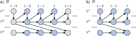
Figure 1: Two illustrations of the same ts-DAG $\mathcal{D}$ that represents a structural process as in eq. (1) of order $p_{\mathcal{D}}=p_{ts}=2$ with three component time series $V^{1}$, $V^{2}$, and $V^{3}$. Given the implicit assertion that there is no edge of length larger than those depicted, the ts-DAG is uniquely specified by showing a segment of $p_{ts}+1$ successive time steps. The horizontal dots indicate that the structure is repeated into the infinite past and infinite future.

3.3 Time series DAGs as causal graphs for structural vector autoregressive processes

Since the structural process in eq. (1) is acyclic by assumption, i.e., since the system of equations is recursive, its causal graph is acyclic (hence the terminology). In combination with the discussions in the previous subsection we thus get the following result.

Lemma 3.5.

The causal graph of an acyclic and causally stationary structural vector autoregressive process as in eq. (1) is a ts-DAG.

This observation has been made before, for example in Runge et al. (2012) and Peters, Janzing and Schölkopf (2013) where ts-DAGs have respectively been called time series graphs and full time graphs. We note that, because of time order, the assumption of acyclicity restricts only the ts-DAG’s contemporaneous edges.

In the non-time series setting, an acyclic SCM defines a unique distribution over the SCM’s variables (pushforward of the noise distribution by the structural assignments). According to the causal Markov condition, see Spirtes, Glymour and Scheines (2000), the SCM’s causal graph is a Bayesian network for this so-called entailed distribution (Pearl, 2009), which in turn implies that $d$-separations (see Pearl (1988), denoted by ‘$\perp\!\!\!\perp$’) in the causal graph imply the corresponding independencies in the distribution (Verma and Pearl, 1990; Geiger, Verma and Pearl, 1990). The causal faithfulness condition, see Spirtes, Glymour and Scheines (2000), assumes the reverse implication, i.e., that all independencies imply the corresponding $d$-separations. Then, $d$-separations and independencies are in one-to-one correspondence.

Although acyclic, the time series setting specified by eq. (1) is more complicated: Since time is indexed by $t\in\mathbb{Z}$ (as opposed to, e.g., $t\in\mathbb{N}$), there is no initial “starting” distribution that can be pushforwarded to explicitly define a unique entailed distribution. Instead, we need to ask whether eq. (1) implicitly defines a distribution; and if yes, how many. Following the terminology in Bongers, Blom and Mooij (2018), this question asks for solutions to eq. (1), that is, for stochastic processes which satisfy eq. (1) almost surely. The existence of such solutions as well as their uniqueness (up to almost sure equality) and properties are non-trivial and not considered here. Rather, for the purpose of this paper we assume that eq. (1) is solved by a (not necessarily unique) strictly stationary stochastic process whose finite-dimensional distributions satisfy the causal Markov and causal faithfulness condition with respect to its ts-DAG. This assumption is common in the literature, cf. Entner and Hoyer (2010), Malinsky and Spirtes (2018), Gerhardus and Runge (2020), and is here only needed for the connection to causality. The results of the present paper are, technically, about marginalizing the independence (i.e., $d$-separation) models of ts-DAGs and remain valid also without that additional assumption. The issue of solving eq. (1) is an important aspect to consider in future work.

3.4 Time series DMAGs

In most real-world scenarios, unobserved common causes cannot be excluded. As mentioned in Sec. 1 for the non-time series setting, directed maximal ancestral graphs (DMAGs) are often used for causal modeling in the presence of unobserved variables. This use of DMAGs as causal graphical models was pioneered in Richardson and Spirtes (2002), which defines a marginalization / projection procedure that from a DAG $\mathcal{G}$ over vertices $\mathbf{V}$, of which only a subset $\mathbf{O}\subseteq\mathbf{V}$ is observed, constructs a DMAG $\mathcal{M}_{\mathbf{O}}(\mathcal{D})$ over the observed variables $\mathbf{O}$ only (see also Zhang (2008a)). The projection of $\mathcal{D}$ to $\mathcal{M}_{\mathbf{O}}(\mathcal{D})$ has two properties: First, both graphs have the same ancestral relationships among vertices in $\mathbf{O}$. Second, $d$-separations in $\mathcal{D}$ among vertices in $\mathbf{O}$ are in one-to-one correspondence to the similar concept of $m$-separation in $\mathcal{M}_{\mathbf{O}}(\mathcal{D})$ (also denoted by ‘$\perp\!\!\!\perp$’). These two properties ensure that if $\mathcal{D}$ is a causal graph then also $\mathcal{M}_{\mathbf{O}}(\mathcal{D})$ carries causal meaning and can be used for causal reasoning as explained in Zhang (2008a).

Below, we generalize the construction of such “causal” DMAGs to the time series setting. To begin, we first note that for time series there are two types of unobserved variables:

• Unobservable variables: Some component time series $L^{1},\dots,L^{n_{L}}$ with $0\leq n_{L}<n_{V}$ may be unobserved entirely by the experimental setup. We call these $L^{i}$ unobservable and call the other component time series $O^{1},\dots,O^{n_{O}}$ with $n_{O}=n_{V}-n_{l}\leq\infty$ observable. The variable index set $\mathbf{I}$ of the ts-DAG $\mathcal{D}$ accordingly decomposes as $\mathbf{I}=\mathbf{I}_{\mathbf{O}}\,\dot{\cup}\,\mathbf{I}_{\mathbf{L}}$. This first type of unobserved variables is similar to the case of unobserved variables in the non-time series setting.

• Temporally unobserved variables: In addition, throughout the paper we will treat only a finite number of time steps $\mathbf{T}_{\mathbf{O}}$ as observed. This construction is specific to the time series setting and means that at times $\mathbf{T}\setminus\mathbf{T}_{\mathbf{O}}$ also the observable time series are treated as unobserved. The rational for doing so is that in practice only finitely many observations are available and hence one can only reason about DMAGs of finite temporal extension.

Throughout the paper we restrict the set $\mathbf{T}_{\mathbf{O}}$ of observed time steps to take one of the following two forms:

• Regular sampling: All time steps within a time interval $[t-p,t]$ for some non-negative integer $p<\infty$ and a reference time step $t$ are observed, i.e., $\mathbf{T}_{\mathbf{O}}=\{t-\tau~{}|~{}0\leq\tau\leq p\}$.

• Regular subsampling: Every $n$-th time step, for $n\geq 2$ an integer, within $[t-p,t]$ with $p<\infty$ is observed, i.e., $\mathbf{T}_{\mathbf{O}}=\{t-\tau~{}|~{}0\leq\tau\leq p,\,\tau\!\!\mod n=0\}$.

The time window length $p$ is not restricted relative to the order $p_{ts}$ of the data-generating process, i.e., we allow all of $p<p_{ts}$ and $p=p_{ts}$ and $p>p_{ts}$. The reference time step $t$ is arbitrary since the ts-DAG $\mathcal{D}$ has repeating edges. We are led to the following definition.

Definition 3.6 (Time series DMAG).

Let $\mathcal{D}=(\mathbf{V},\mathbf{E})$ be a ts-DAG with variable index set $\mathbf{I}$, let $\mathbf{I}_{\mathbf{O}}\subseteq\mathbf{I}$, and let $\mathbf{T}_{\mathbf{O}}\subsetneq\mathbb{Z}$ be regularly sampled or regularly subsampled. The time series DMAG implied by $\mathcal{D}$ over $\mathbf{O}=\mathbf{I}_{\mathbf{O}}\times\mathbf{T}_{\mathbf{O}}$, denoted as $\mathcal{M}_{\mathbf{O}}(\mathcal{D})$ or $\mathcal{M}_{\mathbf{I}_{\mathbf{O}}\times\mathbf{T}_{\mathbf{O}}}(\mathcal{D})$ and also referred to as a ts-DMAG, is the DMAG on the vertex set $\mathbf{O}$ that is obtained by applying the MAG latent projection defined in Zhang (2008a, pp. 1442–3) to $\mathcal{D}$ with $\mathbf{L}=\mathbf{V}\setminus\mathbf{O}$ being the set of latent vertices.

Figure 2 illustrates the construction of ts-DMAGs as projections of ts-DAGs. We stress that all vertices prior to the observed time window (i.e., before time $t-p$) are treated as unobserved, even if they are observable and hence would be observed for a larger value of $p$.

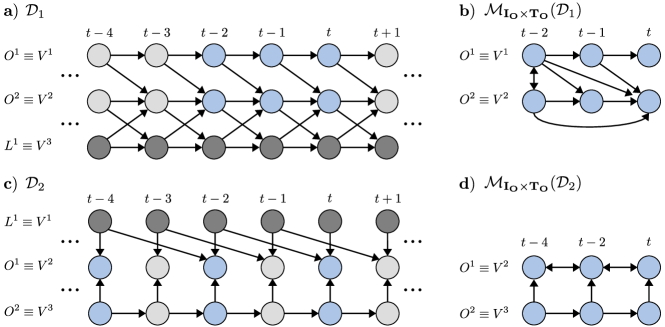
Figure 2: The ts-DAG $\mathcal{D}_{1}$ in part a) implies the ts-DMAG $\mathcal{M}_{\mathbf{I}_{\mathbf{O}}\times\mathbf{T}_{\mathbf{O}}}(\mathcal{D}_{1})$ in part b) for $\mathbf{I}_{\mathbf{O}}=\{1,2\}$ and $\mathbf{T}_{\mathbf{O}}=\{t-2,t-1,t\}$ (regular sampling). The ts-DAG $\mathcal{D}_{2}$ in part c) implies the ts-DMAG $\mathcal{M}_{\mathbf{I}_{\mathbf{O}}\times\mathbf{T}_{\mathbf{O}}}(\mathcal{D}_{2})$ in part d) for $\mathbf{I}_{\mathbf{O}}=\{2,3\}$ and $\mathbf{T}_{\mathbf{O}}=\{t-4,t-2,t\}$ (regular subsampling). Color coding: Observed vertices are light blue, unobservable vertices are dark gray, temporally unobserved observable vertices are light gray.

Remark (on Def. 3.6).

The time series DMAG $\mathcal{M}_{\mathbf{O}}(\mathcal{D})$ is defined as the MAG latent projection of an infinite object, namely of the ts-DAG $\mathcal{D}$. An implementation of this projection in a procedure that always terminates in finite time is possible but non-trivial. Such a procedure will be discussed in Gerhardus et al. (2023). For the present paper, however, this procedure is not needed because all theoretical results and examples either do not require the explicit construction of ts-DMAGs or one can carry out the required projections by hand.

Time series DMAGs are the central objects of interest in this paper and a significant part of the paper deals with deriving their properties. We will see that the repeating edges property of ts-DAGs $\mathcal{D}$ plays an essential role in this regard. As a first step, the following lemma notes which of the defining properties of ts-DAGs carry over to ts-DMAGs.

Lemma 3.7.

Let $\mathcal{M}_{\mathbf{O}}(\mathcal{D})$ be a ts-DMAG. Then:

1. $\mathcal{M}_{\mathbf{O}}(\mathcal{D})$ has a time series structure.

2. $\mathcal{M}_{\mathbf{O}}(\mathcal{D})$ is time ordered.

3. There are cases in which $\mathcal{M}_{\mathbf{O}}(\mathcal{D})$ does not have repeating edges.

While according to part 1 of Lemma 3.7 every ts-DMAG is a DMAG with time series structure, part 2 implies that the reverse is not true. Namely, DMAGs with time series structure that are not time ordered cannot be ts-DMAGs. We thus see that ts-DMAGs are a proper subclass of DMAGs with time series structure. The following example shows that ts-DMAGs $\mathcal{M}_{\mathbf{O}}(\mathcal{D})$ do not in general have repeating edges.

Example 3.8.

The ts-DMAG in part b) of Fig. 2 does not have repeating edges because there is the edge $O^{1}_{t-2}{\leftrightarrow}O^{2}_{t-2}$ although $O^{1}_{t-1}$ and $O^{2}_{t-1}$ (and $O^{1}_{t}$ and $O^{2}_{t}$) are non-adjacent.

Despite this fact, the repeating edges property of the ts-DAG $\mathcal{D}$ strongly restricts the connectivity pattern of the ts-DMAG $\mathcal{M}_{\mathbf{O}}(\mathcal{D})$. We will work out these restrictions in Sec. 4.

4 Characterization of ts-DMAGs

The main goal of this section is to characterize the space of ts-DMAGs, i.e., to find conditions that specify exactly which DMAGs with time series structure are ts-DMAGs. Theorem 1 in Sec. 4.6 achieves this goal by providing a single condition that is both necessary and sufficient. The theorem uses the notion of canonical ts-DAGs, see Def. 4.11 in Sec. 4.5. In Sec. 4.4 we introduce stationarified ts-DMAGs and, more generally, the concept of stationarification. This concept simplifies the definition of canonical ts-DAGs and is useful to describe the output of two recent time series causal discovery algorithms (see Sec. 5.5). In Sec. 4.8 we show that ts-DMAGs constitute a strict subset of the classes of graphical models that have so far been used in the literature for describing time lag specific causal relationships and independencies in time series with latent confounders. Section 4.3 discusses several properties that ts-DMAGs necessarily have, but which can also be obeyed by DMAGs that are not ts-DMAGs. These properties are useful for the discussions in Secs. 4.8 and 5. In Sec. 4.2 we show that regular sampling and regular subsampling are equivalent from a graphical point of view. Section 4.7 gives a characterization of the space of stationarified ts-DMAGs. At first, however, we spell out the motivation for the analysis.

4.1 Motivation

When using a class of graphs to represent causal knowledge, it is desirable to know which graphs belong to this class and which do not. Otherwise, it is impossible to fully characterize which causal claims a given graph of that class conveys. Another, a posteriori motivation has been mentioned in the previous paragraph: In Sec. 4.8 we will see that ts-DMAGs are a strict subset of the previously employed model classes. Thus, when using ts-DMAGs as targets of inference in causal discovery or to reason about causal effects, it is, respectively, possible to learn more qualitative causal relationships (see Secs. 5.4 and 5.5 for an in-depth discussion) and to identify more causal effects (see Example 5.8) from data without having imposed any additional assumption or restriction.

4.2 Equivalence of regular subsampling and regular sampling

In Sec. 3.4 we restricted the set of observed time steps $\mathbf{T}_{\mathbf{O}}$ to regular sampling or regular subsampling. While different at first sight, these two cases are equivalent in the following sense.

Lemma 4.1.

Let $\mathcal{D}$ be a ts-DAG and $1\leq n_{\text{steps}}\in\mathbb{N}$. For $1\leq n\in\mathbb{Z}$ define the set $\mathbf{T}_{\mathbf{O}}^{n}=\{t-m\cdot n~{}|~{}0\leq m\leq n_{\text{steps}}-1\}$. Then, with equality up to relabeling vertices:

1. For every $n>1$ there is a ts-DAG $\mathcal{D}^{\prime}$ such that $\mathcal{M}_{\mathbf{I}_{\mathbf{O}}\times\mathbf{T}_{\mathbf{O}}^{n}}(\mathcal{D})=\mathcal{M}_{\mathbf{I}_{\mathbf{O}}\times\mathbf{T}_{\mathbf{O}}^{1}}(\mathcal{D}^{\prime})$.

2. For every $n>1$ there is a ts-DAG $\mathcal{D}^{\prime}$ such that $\mathcal{M}_{\mathbf{I}_{\mathbf{O}}\times\mathbf{T}_{\mathbf{O}}^{1}}(\mathcal{D})=\mathcal{M}_{\mathbf{I}_{\mathbf{O}}\times\mathbf{T}_{\mathbf{O}}^{n}}(\mathcal{D}^{\prime})$.

Lemma 4.1 implies: Every property that ts-DMAGs necessarily have in case of regular sampling is also necessarily obeyed in case of regular subsampling (part 1) and vice versa (part 2). Moreover, every set of additional properties that, when imposed on a DMAG $\mathcal{M}$ with time series structure, is sufficient for $\mathcal{M}$ to be a ts-DMAG in case of regular sampling is also sufficient in case of regular subsampling (part 2) and vice versa (part 1).

Due to this equivalence we from here on restrict to regular sampling, without losing generality, and write $\mathcal{M}^{p}(\mathcal{D})$ for $\mathcal{M}_{\mathbf{O}}(\mathcal{D})$ where $\mathbf{O}=\mathbf{I}_{\mathbf{O}}\times\mathbf{T}_{\mathbf{O}}$ and $\mathbf{T}_{\mathbf{O}}=\{t-\tau~{}|~{}0\leq\tau\leq p\}$.

4.3 Properties of ts-DMAGs

In this subsection, we discuss several properties that ts-DMAGs $\mathcal{M}^{p}(\mathcal{D})$ necessarily have. These properties are such that a certain graphical property persists when the involved vertices are shifted in time. We use the following definitions.

Definition 4.2 (Time-shift persistent graphical properties).

A partial mixed graph $\mathcal{G}=(\mathbf{V},\mathbf{E})$ with time series structure has$\ldots$

1. $\ldots$ repeating adjacencies if the following holds: If $((i,t_{i}),(j,t_{j}))\in\mathbf{E}$ and $(i,t_{i}+\Delta t),(j,t_{j}+\Delta t)\in\mathbf{V}$ then $((i,t_{i}+\Delta t),(j,t_{j}+\Delta t))\in\mathbf{E}$.

2. $\ldots$ past-repeating adjacencies if the following holds: If $((i,t_{i}),(j,t_{j}))\in\mathbf{E}$ and $(i,t_{i}+\Delta t),(j,t_{j}+\Delta t)\in\mathbf{V}$ with $\Delta t<0$ then $((i,t_{i}+\Delta t),(j,t_{j}+\Delta t))\in\mathbf{E}$.

3. $\ldots$ repeating orientations if the following holds: If $((i,t_{i}),(j,t_{j}))\in\mathbf{E}_{\bullet}$ with $\bullet\in\{{\rightarrow},{\leftrightarrow},{\circ\!{\rightarrow}},$ ${\circ\!{\--}\!\circ}\}$ and $((i,t_{i}+\Delta t),(j,t_{j}+\Delta t))\in\mathbf{E}$ then $((i,t_{i}+\Delta t),(j,t_{j}+\Delta t))\in\mathbf{E}_{\bullet}$.

A DMAG $\mathcal{M}=(\mathbf{V},\mathbf{E})$ with time series structure has

1. $\ldots$ repeating ancestral relationships if the following holds: If $(i,t_{i})\in an((j,t_{j}),\mathcal{M})$ and $(i,t_{i}+\Delta t),(j,t_{j}+\Delta t)\in\mathbf{V}$ then $(i,t_{i}+\Delta t)\in an((j,t_{j}+\Delta t),\mathcal{M})$.

2. $\ldots$ repeating separating sets if the following holds: If $(i,t_{i})\perp\!\!\!\perp(j,t_{j})~{}|~{}\mathbf{S}$ and $\{(i,t_{i}+\Delta t),(j,t_{j}+\Delta t)\}\cup\mathbf{S}_{\Delta t}\subseteq\mathbf{V}$, where $\mathbf{S}_{\Delta t}$ is obtained by shifting every vertex in $\mathbf{S}$ by $\Delta t$ time steps, then $(i,t_{i}+\Delta t)\perp\!\!\!\perp(j,t_{j}+\Delta t)~{}|~{}\mathbf{S}_{\Delta t}$.

Remark (on Def. 4.2).

Section 4 is concerned with DAGs and DMAGs only. However, in Sec. 5 we will apply the concepts of repeating adjacencies, past-repeating adjacencies and repeating orientations also to DPAGs (which are a special case of partial mixed graphs). Hence, we already here formulate the definition in sufficient generality.

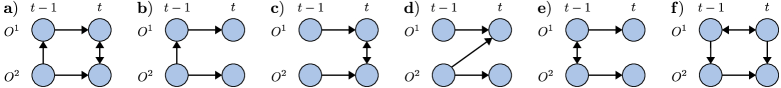
Figure 3: Examples of time ordered DMAGs with time series structure for illustrating the properties from Def. 4.2 and the repeating edges property from Def. 3.3. In each case we state which of these properties apply. a) Repeating adjacencies, repeating separating sets, past-repeating adjacencies. b) Repeating orientations, repeating separating sets, past-repeating adjacencies. c) Repeating orientations, repeating ancestral relationships. d) All but repeating separating sets. e) All but repeating repeating edges and repeating adjacencies. f) All.

Figure 3 illustrates the five properties introduced by Def. 4.2 as well as their distinctions. Below we will make frequent use of the implications expressed by the following lemma.

Lemma 4.3.

1. Repeating edges is equivalent to the combination of repeating adjacencies and repeating orientations.

2. Repeating adjacencies implies past-repeating adjacencies.

3. Repeating ancestral relationships implies repeating orientations.

4. In graphs with time index set $\mathbf{T}=\mathbb{Z}$, repeating edges implies repeating ancestral relationships and repeating separating sets.

These implications further show that the combination of repeating adjacencies and repeating ancestral relationships implies repeating edges. Importantly, repeating orientations does not imply repeating ancestral relationships, see part b) of Fig. 3 for an example.

Since ts-DAGs have repeating edges, according to Lemma 4.3 they in fact also have all five properties given in Def. 4.2. How about ts-DMAGs? While these in general do not inherit repeating edges from the underlying ts-DAG, see part 3 of Lemma 3.7, the following lemma shows that ts-DMAGs do feature some of the weaker time-shift persistent properties.

Lemma 4.4.

1. Time series DMAGs $\mathcal{M}^{p}(\mathcal{D})$ have repeating ancestral relationships.

2. Time series DMAGs $\mathcal{M}^{p}(\mathcal{D})$ have repeating orientations.

3. Time series DMAGs $\mathcal{M}^{p}(\mathcal{D})$ have repeating separating sets.

4. Time series DMAGs $\mathcal{M}^{p}(\mathcal{D})$ have past-repeating adjacencies.

5. There are cases in which a ts-DMAG $\mathcal{M}^{p}(\mathcal{D})$ does not have repeating adjacencies.

The ts-DMAGs in parts b) and d) of Fig. 2 indeed satisfy the properties asserted by parts 1 through 4 of Lemma 4.4. Moreover, part 5 of Lemma 4.4 clarifies why ts-DMAGs may fail to have repeating edges: They do not necessarily have repeating adjacencies but only the weaker property of past-repeating adjacencies. The following example illustrates this fact.

Example 4.5.

Consider the ts-DAG $\mathcal{D}_{1}$ in part a) of Fig. 2. In this graph the $d$-separation $O^{1}_{t+\Delta t}\perp\!\!\!\perp O^{2}_{t+\Delta t}~{}|~{}O^{1}_{t+\Delta t-1}$ holds for all $\Delta t\in\mathbb{Z}$. Hence, the vertices $O^{1}_{t}$ and $O^{2}_{t}$ (and, similarly, $O^{1}_{t-1}$ and $O^{2}_{t-1}$) are non-adjacent in the ts-DMAG $\mathcal{M}^{2}(\mathcal{D}_{1})$ in part b) of the figure. However, since $O^{1}_{t-3}$ is temporally unobserved and the $d$-separation $O^{1}_{t+\Delta t}\perp\!\!\!\perp O^{2}_{t+\Delta t}~{}|~{}\mathbf{S}$ requires that $O^{1}_{t+\Delta t-1}\in\mathbf{S}$, the vertices $O^{1}_{t-2}$ and $O^{1}_{t-2}$ are adjacent in $\mathcal{M}^{2}(\mathcal{D}_{1})$.

That ts-DMAGs have repeating orientations and repeating separating sets has already been found and used in Entner and Hoyer (2010).

4.4 Stationarified ts-DMAGs

Example 4.5 shows that in a ts-DMAG $\mathcal{M}^{p}(\mathcal{D})$ there may be an edge $(i,t_{i}+\Delta t){\ast\!{\--}\!\ast}(j,t_{j}+\Delta t)$ with $\Delta t<0$ even if the vertices $(i,t_{i})$ and $(j,t_{j})$ are non-adjacent in $\mathcal{M}^{p}(\mathcal{D})$. This is the case even though one then knows that $(i,t_{i}+\Delta t)$ and $(j,t_{j}+\Delta t)$ can be $d$-separated in underlying ts-DAG $\mathcal{D}$, just not by a set of vertices that is within the observed time window. One might thus view such an edge $(i,t_{i}+\Delta t){\ast\!{\--}\!\ast}(j,t_{j}+\Delta t)$ in $\mathcal{M}^{p}(\mathcal{D})$ as an artifact of the chosen time window and hence prefer to manually remove the edge by subjecting the ts-DMAG to the following operation.

Definition 4.6 (Stationarification).

Let $\mathcal{G}=(\mathbf{V},\mathbf{E})$ be a directed partial mixed graph with time series structure. The stationarification of $\mathcal{G}$, denoted as $stat(\mathcal{G})$, is the graph $stat(\mathcal{G})=(\mathbf{V}^{\prime},\mathbf{E}^{\prime})$ defined as follows:

1. It has the same set of vertices as $\mathcal{G}$, i.e., $\mathbf{V}^{\prime}=\mathbf{V}$.

2. There is an edge $((i,t_{i}),(j,t_{j}))\in\mathbf{E}^{\prime}_{\bullet}$ with $\bullet\in\{{\rightarrow},\,{\leftrightarrow},\,{\circ\!{\rightarrow}},\,{\circ\!{\--}\!\circ}\}$ if and only if $((i,t_{i}+\Delta t),(j,t_{j}+\Delta t))\in\mathbf{E}_{\bullet}$ in $\mathcal{G}$ for all $\Delta t$ with $(i,t_{i}+\Delta t),(j,t_{j}+\Delta t)\in\mathbf{V}$.

Remark (on Def. 4.6).

Section 4 is concerned with DAGs and DMAGs only. In these graphs there are by definition no edges of the types ${\circ\!{\rightarrow}}$ or ${\circ\!{\--}\!\circ}$. However, in Sec. 5 we will apply the concept of sationarification also to DPAGs. Since these graphs (DPAGs) can contain edges ${\circ\!{\rightarrow}}$ or ${\circ\!{\--}\!\circ}$, we already here formulate the definition in sufficient generality.

To see that the process of stationarification indeed achieves what it is supposed to do, consider the ts-DMAG $\mathcal{M}_{1}$ in part a) of Fig. 4. In this graph there is the edge $O^{1}_{t-2}{\leftrightarrow}O^{2}_{t-2}\in\mathbf{E}_{{\leftrightarrow}}$ while the vertices $O^{1}_{t-1}$ and $O^{2}_{t-1}$ (and, similarly, $O^{1}_{t}$ and $O^{2}_{t}$) are non-adjacent. According to part 2 of Def. 4.6 (note the “for all $\Delta t$”), the vertices $O^{1}_{t-2}$ and $O^{2}_{t-2}$ are therefore non-adjacent in the stationarification $stat(\mathcal{M}_{1})$ of $\mathcal{M}_{1}$ as shown in part b) of Fig. 4.

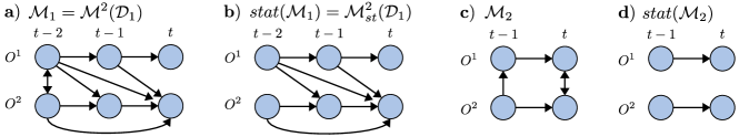
Figure 4: A ts-DMAG $\mathcal{M}_{1}=\mathcal{M}^{2}(\mathcal{D}_{1})$ (the same as in part b) of Fig. 2) and a DMAG with time series structure $\mathcal{M}_{2}$ (the same as in part a) of Fig. 3) together with their stationarifications. Note that although $\mathcal{M}_{2}$ has repeating adjacencies its contemporaneous edges are not in $stat(\mathcal{M}_{2})$ because these edges do not have the same orientation.

Stationarification removes an edge $(i,t_{i}+\Delta t){\ast\!{\--}\!\ast}(j,t_{j}+\Delta t)$ also if $(i,t_{i})$ and $(j,t_{j})$ are adjacent but if the edges $(i,t_{i}){\ast\!{\--}\!\ast}(j,t_{j})$ and $(i,t_{i}+\Delta t){\ast\!{\--}\!\ast}(j,t_{j}+\Delta t)$ have different orientations (note the “$\bullet$” subscripts on $\mathbf{E}^{\prime}_{\bullet}$ and $\mathbf{E}_{\bullet}$ in part 2 of Def. 4.6). This effect, illustrated by parts c) and d) of Fig. 4, ensures that $stat(\mathcal{G})$ is the unique largest subgraph of $\mathcal{G}$ with repeating edges. For graphs with repeating orientations (as, e.g., ts-DMAGs) this effect does not occur and stationarification only concerns adjacencies (as, e.g., in parts a) and b) of Fig. 4).

Since ts-DMAGs $\mathcal{M}^{p}(\mathcal{D})$ have repeating orientation and past-repeating adjacencies, their stationarifications $stat(\mathcal{M}^{p}(\mathcal{D}))$ can be characterized with the following simpler condition.

Lemma 4.7.

The stationarification $stat(\mathcal{M}^{p}(\mathcal{D}))$ of a ts-DMAG $\mathcal{M}^{p}(\mathcal{D})$ is the unique subgraph of $\mathcal{M}^{p}(\mathcal{D})$ in which the vertices $(i,t_{j}-\tau)$ and $(j,t_{j})$ with $\tau\geq 0$ are adjacent if and only if the vertices $(i,t-\tau)$ and $(j,t)$ are adjacent in $\mathcal{M}^{p}(\mathcal{D})$.

Because the stationarification $stat(\mathcal{G})$ is a subgraph of $\mathcal{G}$, a time series structure and time order naturally carry over from $\mathcal{G}$ to $stat(\mathcal{G})$. Moreover, we can prove the following.

Lemma 4.8.

The stationarification $stat(\mathcal{M}^{p}(\mathcal{D}))$ of a ts-DMAG $\mathcal{M}^{p}(\mathcal{D})$ is a DMAG.

We thus refer to $stat(\mathcal{M}^{p}(\mathcal{D}))$ as a stationarified ts-DMAG and abbreviate $stat(\mathcal{M}^{p}(\mathcal{D}))$ as $\mathcal{M}_{st}^{p}(\mathcal{D})$. However, as the following example shows, a stationarified ts-DMAG $\mathcal{M}_{st}^{p}(\mathcal{D})$ may not be the MAG latent projection of any ts-DAG, i.e., may not be a ts-DMAG.

Example 4.9.

The stationarified ts-DMAG $\mathcal{M}^{2}_{st}(\mathcal{D}_{1})$ in part b) of Fig. 4 implies the $d$-separation $O^{1}_{t-2}\perp\!\!\!\perp O^{2}_{t-2}$ and the $d$-connections $O^{1}_{t-1}{\cancel{\,\,\perp\!\!\!\perp}\,}O^{2}_{t-1}$ and $O^{1}_{t}{\cancel{\,\,\perp\!\!\!\perp}\,}O^{2}_{t}$. The graph $\mathcal{M}^{2}_{st}(\mathcal{D}_{1})$ does thus not have repeating separating sets and can, by means of Lemma 4.4, not be a ts-DMAG. Also note that in the underlying ts-DAG $\mathcal{D}_{1}$, shown in part a) of Fig. 2, the $d$-connection $O^{1}_{t-2}{\cancel{\,\,\perp\!\!\!\perp}\,}O^{2}_{t-2}$ holds. From this observation we learn that $(i,t_{i})\perp\!\!\!\perp(j,t_{j})~{}|~{}\mathbf{S}$ in $\mathcal{M}_{st}^{p}(\mathcal{D})$ does not necessarily imply $(i,t_{i})\perp\!\!\!\perp(j,t_{j})~{}|~{}\mathbf{S}$ in $\mathcal{D}$.

The vertices $(i,t-\tau_{i})$ and $(j,t-\tau_{j})$ with $0\leq\tau_{j}\leq\tau_{i}\leq p$ are adjacent in a stationarified ts-DMAG $\mathcal{M}_{st}^{p}(\mathcal{D})$ if and only if they can not be $d$-separated by any set of observable vertices within $[t-p-\tau_{j},t]$ in the underlying ts-DAG $\mathcal{D}$ (instead of $[t-p,t]$, which is what a ts-DMAG would assert). The orientation of edges, however, retains the standard meaning: Tail and head marks respectively convey (non-)ancestorship according to the ts-DAG $\mathcal{D}$. The following lemma says that stationarification does not change ancestral relationships.

Lemma 4.10.

The ts-DMAG $\mathcal{M}^{p}(\mathcal{D})$ and its stationarification $\mathcal{M}_{st}^{p}(\mathcal{D})$ agree on ancestral relationships, i.e., $(i,t_{i})\in an((j,t_{j}),\mathcal{M}^{p}(\mathcal{D}))$ if and only if $(i,t_{i})\in an((j,t_{j}),\mathcal{M}_{st}^{p}(\mathcal{D}))$.

Since $\mathcal{M}^{p}(\mathcal{D})$ and $\mathcal{D}$ by construction of the MAG latent projection agree on ancestral relationships, Lemma 4.10 implies that also the stationarified ts-DMAG $\mathcal{M}_{st}^{p}(\mathcal{D})$ agrees with the ancestral relationships of $\mathcal{D}$. Thus, $\mathcal{M}_{st}^{p}(\mathcal{D})$ has repeating ancestral relationships.

In summary, edges in the ts-DMAG $\mathcal{M}^{p}(\mathcal{D})$ that are not also in $\mathcal{M}_{st}^{p}(\mathcal{D})$ are due to marginalizing over observable vertices before $t-p$. Such edges disappear when $p$ is sufficiently increased, see also Gerhardus (2023, Sec. B.8). However, as we will show in Sec. 5.3, these additional edges play a useful role in causal discovery. In Sec. 5.5 we will further use the concept of stationarification to describe the SVAR-FCI causal discovery algorithm from Malinsky and Spirtes (2018) and the LPCMCI causal discovery algorithm from Gerhardus and Runge (2020).

4.5 Canonical ts-DAGs

In the current subsection we return to the goal of characterizing the space of ts-DMAGs. To this end, we first recall the concept of canonical DAGs.

Definition 4.11 (Canonical DAG. From Sec. 6.1 of Richardson and Spirtes (2002), specialized to the case of directed ancestral graphs).

Let $\mathcal{G}=(\mathbf{V},\mathbf{E})$ be a directed ancestral graph. The canonical DAG $\mathcal{D}_{c}(\mathcal{G})$ of $\mathcal{G}$ is the graph $\mathcal{D}_{c}(\mathcal{G})=(\mathbf{V}^{ca},\mathbf{E}^{ca})$ defined as follows:

1. Its vertex set is $\mathbf{V}^{ca}=\mathbf{V}\cup\mathbf{L}$, where $\mathbf{L}=\{l_{ij}~{}|~{}(i,j)\in\mathbf{E}_{{\leftrightarrow}}\}$.

2. Its edge set $\mathbf{E}^{ca}=\mathbf{E}^{ca}_{\rightarrow}$ consists of the edges

   • $i{\rightarrow}j$ for all $(i,j)\in\mathbf{E}_{{\rightarrow}}$ and

   • $l_{ij}{\rightarrow}i$ for all $l_{ij}\in\mathbf{L}$ and

   • $l_{ij}{\rightarrow}j$ for all $l_{ij}\in\mathbf{L}$.

Intuitively, the canonical DAG $\mathcal{D}_{c}(\mathcal{G})$ of a directed ancestral graph $\mathcal{G}$ is obtained by replacing each bidirected edge $i{\leftrightarrow}j$ in $\mathcal{G}$ with $i{\leftarrow}l_{ij}{\rightarrow}j$ where $l_{ij}$ is an additionally inserted, unobserved vertex. The canonical DAG $\mathcal{D}_{c}(\mathcal{G})$ is a DAG and has the convenient property that there are no edges pointing into unobserved vertices and hence that there are also no edges between two unobserved vertices. Despite this simple structure of unobserved vertices, the following result shows that canonical DAGs are expressive enough to generate all DMAGs.

Lemma 4.12 (Theorem 6.4 in Richardson and Spirtes (2002), specialized to directed ancestral graphs).

If $\mathcal{M}$ is a DMAG over vertex set $\mathbf{O}$, then the MAG latent projection $\mathcal{M}_{\mathbf{O}}(\mathcal{D}_{c}(\mathcal{M}))$ of the canonical DAG $\mathcal{D}_{c}(\mathcal{M})$ of $\mathcal{M}$ equals $\mathcal{M}$, i.e., $\mathcal{M}=\mathcal{M}_{\mathbf{O}}(\mathcal{D}_{c}(\mathcal{M}))$.

Lemma 4.12 means that every DMAG is the MAG latent projection of some DAG. Moreoever, the condition $\mathcal{M}=\mathcal{M}_{\mathbf{O}}(\mathcal{D}_{c}(\mathcal{M}))$ yields a characterization of DMAGs in the sense that a directed ancestral graph $\mathcal{G}$ is a DMAG if and only if it meets the condition $\mathcal{G}=\mathcal{M}_{\mathbf{O}}(\mathcal{D}_{c}(\mathcal{G}))$. Because DMAGs are already characterized by definition, the alternative characterization by the condition $\mathcal{G}=\mathcal{M}_{\mathbf{O}}(\mathcal{D}_{c}(\mathcal{G}))$ is of limited use in this case.

For ts-DMAGs, however, there is no definitional characterization. In addition, because not every DMAG with time series structure is a ts-DMAG (see the explanation below Lemma 3.7), characterizing ts-DMAGs is a non-trivial task. In the remaining parts of the current subsection and Sec. 4.6, we show that ts-DMAGs can be characterized by an appropriate generalization of the condition $\mathcal{G}=\mathcal{M}_{\mathbf{O}}(\mathcal{D}_{c}(\mathcal{G}))$. The first step of such a generalization is to find an appropriate generalization of canonical DAGs.

The generalization of canonical DAGs to the time series setting is non-trivial for the following reason. Consider an edge $(i,t_{i}){\ast\!{\--}\!\ast}(j,t_{j})$ in a DMAG $\mathcal{M}$ with time series structure that is not in the DMAG’s stationarification $stat(\mathcal{M})$. If, depending on the orientation of the edge $(i,t_{i}){\ast\!{\--}\!\ast}(j,t_{j})$ in $\mathcal{M}$, either $(i,t_{i}){\rightarrow}(j,t_{j})$ or $(i,t_{i}){\leftarrow}(j,t_{j})$ or $(i,t_{i}){\leftarrow}(l_{ij},t_{ij}){\rightarrow}(j,t_{j})$ with $(l_{ij},t_{ij})$ unobserved were included in a “canonical ts-DAG” $\mathcal{D}_{c}(\mathcal{M})$, then the repeating edges property of ts-DAGs would require the same structure to be present at all other time steps too. Hence, in $\mathcal{D}_{c}(\mathcal{M})$ there would be $(i,t_{i}+\Delta t){\rightarrow}(j,t_{j}+\Delta t)$ or $(i,t_{i}+\Delta t){\leftarrow}(j,t_{j}+\Delta t)$ or $(i,t_{i}+\Delta t){\leftarrow}(l_{ij},t_{ij}+\Delta t){\rightarrow}(j,t_{j}+\Delta t)$ for all $\Delta t\in\mathbb{Z}$. Consequently, in the MAG latent projection $\mathcal{M}_{\mathbf{O}}(\mathcal{D}_{c}(\mathcal{M}))$ of $\mathcal{D}_{c}(\mathcal{M})$ there would be an edge $(i,t_{i}+\Delta t){\ast\!{\--}\!\ast}(j,t_{j}+\Delta t)$ of the same type for all $\Delta t$. But then also in the stationarification $stat(\mathcal{M}_{\mathbf{O}}(\mathcal{D}_{c}(\mathcal{M})))$ of $\mathcal{M}_{\mathbf{O}}(\mathcal{D}_{c}(\mathcal{M}))$ there would be the edge $(i,t_{i}+\Delta t){\ast\!{\--}\!\ast}(j,t_{j}+\Delta t)$ for all $\Delta t$. Hence, $\mathcal{M}$ could not equal $\mathcal{M}_{\mathbf{O}}(\mathcal{D}_{c}(\mathcal{M}))$.

Given these considerations, the canonical ts-DAG $\mathcal{D}_{c}(\mathcal{M})$ of a ts-DMAG $\mathcal{M}$ should instead only take into account the edges in the stationarification $stat(\mathcal{M})$ of $\mathcal{M}$. We are thus lead to the following definition, which for use further below is not restricted to ts-DMAGs but more generally applies to acyclic directed mixed graphs.

Definition 4.13 (Canonical ts-DAG).

Let $\mathcal{G}$ be an acyclic directed mixed graph with time series structure and let $\mathbf{V}=\mathbf{I}\times\mathbf{T}$ with $\mathbf{T}=\{t-\tau~{}|~{}0\leq\tau\leq p\}$ be its set of vertices. Denote with $\mathbf{E}^{stat}$ the set of edges of $stat(\mathcal{G})$. The canonical ts-DAG associated to $\mathcal{G}$, denoted as $\mathcal{D}_{c}(\mathcal{G})$, is the graph $\mathcal{D}_{c}(\mathcal{G})=(\mathbf{V}^{ca},\mathbf{E}^{ca})$ defined as follows:

1. Its set of vertices is $\mathbf{V}^{ca}=\left(\mathbf{I}\cup\mathbf{J}\right)\times\mathbb{Z}$, where $\mathbf{J}=\{(i,j,\tau)~{}|~{}((i,t-\tau),(j,t))\in\mathbf{E}^{stat}_{{\leftrightarrow}}\}$. The variable index set is $\mathbf{I}\cup\mathbf{J}$ and the time index set is $\mathbb{Z}$.

2. Its set of edges $\mathbf{E}^{ca}=\mathbf{E}^{ca}_{\rightarrow}$ are for all $\Delta t\in\mathbb{Z}$

   • $(i,t-\tau+\Delta t){\rightarrow}(j,t+\Delta t)$ for all $((i,t-\tau),(j,t))\in\mathbf{E}^{stat}_{{\rightarrow}}$ and

   • $((i,j,\tau),t+\Delta t){\rightarrow}(i,t+\Delta t)$ for all $(i,j,\tau)\in\mathbf{J}$ and

   • $((i,j,\tau),t-\tau+\Delta t){\rightarrow}(j,t+\Delta t)$ for all $(i,j,\tau)\in\mathbf{J}$.

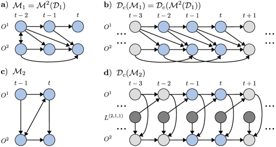
Figure 5: A ts-DMAG $\mathcal{M}_{1}=\mathcal{M}^{2}(\mathcal{D}_{1})$ (the same as in part b) of Fig. 2 and part a) of Fig. 4) and a DMAG with time series structure $\mathcal{M}_{2}$ together with their canonical ts-DAGs. In $\mathcal{D}_{c}(\mathcal{M}_{1})$ there is no unobservable time series because in $\mathcal{M}_{1}$ there is no bidirected edge that is repetitive in time and hence there is no bidirected edge in $stat(\mathcal{M}_{1})$. The unobservable time series $L^{(2,1,1)}$ in $\mathcal{D}_{c}(\mathcal{M}_{2})$ in the notation of Def. 4.13 corresponds to $(2,1,1)\in\mathbf{J}$ and results from the edge $O^{2}_{t-1}{\leftrightarrow}O^{1}_{t}$ in $stat(\mathcal{M}_{2})=\mathcal{M}_{2}$.

Figure 5 illustrates canonical ts-DAGs. Intuitively, the canonical ts-DAG $\mathcal{D}_{c}(\mathcal{G})$ of $\mathcal{G}$ is obtained in three steps: First, replace $\mathcal{G}$ by its stationarification $stat(\mathcal{G})$. Second, in $stat(\mathcal{G})$ replace every bidirected edge $(i,t_{j}-\tau){\leftrightarrow}(j,t_{j})$ with $(i,t_{j}-\tau){\leftarrow}((i,j,\tau),t_{j}-\tau){\rightarrow}(j,t_{j})$ where $((i,j,\tau),t_{j}-\tau)$ is an additionally inserted, unobserved vertex. Third, repeat this structure into the infinite past and future according to the repeating edges property. This intuition identifies the vertices $((i,j,\tau),s)$ with $(i,j,\tau)\in\mathbf{J}$ and $s\in\mathbb{Z}$ as analogs of the unobserved vertices $l_{ij}\in\mathbf{L}$ in standard canonical DAGs (see Def. 4.11 above) and, in addition, means that the time series indexed by $\mathbf{J}$ are treated as unobservable. The key difference between standard canonical DAGs and canonical ts-DAGs is the first of the three steps, i.e., the application of stationarification. A similarity is that also in canonical ts-DAGs there are no edges into unobservable vertices and hence no edges between two unobservable vertices.

Canonical ts-DAGs are indeed ts-DAGs and, by means of the following result, yield the desired generalization of Lemma 4.12.

Lemma 4.14.

Let $\mathcal{D}$ be a ts-DAG with variable index set $\mathbf{I}$. Let $\mathbf{I}_{\mathbf{O}}\subseteq\mathbf{I}$ and $\mathbf{T}_{\mathbf{O}}=\{t-\tau~{}|~{}0\leq\tau\leq p\}$ with $p\geq 0$. Then, $\mathcal{M}_{\mathbf{O}}(\mathcal{D})=\mathcal{M}_{\mathbf{O}}(\mathcal{D}_{c}(\mathcal{M}_{\mathbf{O}}(\mathcal{D})))$ with $\mathbf{O}=\mathbf{I}_{\mathbf{O}}\times\mathbf{T}_{\mathbf{O}}$.

Remark (on Lemma 4.14).

The lemma involves two different MAG latent projections: First, the projection of the ts-DAG $\mathcal{D}$ to the ts-DMAG $\mathcal{M}_{\mathbf{O}}(\mathcal{D})$. Second, the projection of the canonical ts-DAG $\mathcal{D}_{c}(\mathcal{M}_{\mathbf{O}}(\mathcal{D}))$ of $\mathcal{M}_{\mathbf{O}}(\mathcal{D})$ to $\mathcal{M}_{\mathbf{O}}(\mathcal{D}_{c}(\mathcal{M}_{\mathbf{O}}(\mathcal{D})))$. In the first projection, the time series indexed by $\mathbf{I}\setminus\mathbf{I}_{\mathbf{O}}$ are unobservable. In the second projection, the time series indexed by the set $\mathbf{J}$ are unobservable. In both projections, all vertices before $t-p$ and after $t$ are temporally unobserved. However, since the set of observed variables is the same in both projections (namely $\mathbf{O}$), no confusion arises when writing $\mathcal{M}^{p}(\mathcal{D})=\mathcal{M}^{p}(\mathcal{D}_{c}(\mathcal{M}^{p}(\mathcal{D})))$ instead of $\mathcal{M}_{\mathbf{O}}(\mathcal{D})=\mathcal{M}_{\mathbf{O}}(\mathcal{D}_{c}(\mathcal{M}_{\mathbf{O}}(\mathcal{D})))$. From here on we adopt this notation.

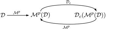
Figure 6: Conceptual illustration of Lemma 4.14.

Lemma 4.14 says that the composition of creating the canonical ts-DAG and then projecting back to the original vertices is the identity operation on the space of ts-DMAGs, see Fig. 6. This result is far from obvious for two reasons: First, if an edge $(i,t_{i}){\ast\!{\--}\!\ast}(j,t_{j})$ in a ts-DMAG $\mathcal{M}^{p}(\mathcal{D})$ is not in the stationarified ts-DMAG $\mathcal{M}_{st}^{p}(\mathcal{D})$ then in the canonical ts-DAG $\mathcal{D}_{c}(\mathcal{M}^{p}(\mathcal{D}))$ there is neither $(i,t_{i}){\rightarrow}(j,t_{j})$ nor $(i,t_{i}){\leftarrow}(j,t_{j})$ nor $(i,t_{i}){\leftarrow}(l_{ij},t_{ij}){\rightarrow}(j,t_{j})$ with $(l_{ij},t_{ij})$ unobservable. Hence, the edge $(i,t_{i}){\ast\!{\--}\!\ast}(j,t_{j})$ needs to appear in the MAG latent projection $\mathcal{M}^{p}(\mathcal{D}_{c}(\mathcal{M}^{p}(\mathcal{D})))$ of $\mathcal{D}_{c}(\mathcal{M}^{p}(\mathcal{D}))$ in a non-trivial way, namely because of marginalizing over the temporally unobserved vertices. Second, this marginalization over the vertices before $t-p$ must not create superfluous edges.

Example 4.15.

The example in Fig. 7 illustrates Lemma 4.14. This example also shows that the original ts-DAG $\mathcal{D}$ and the canonical ts-DAG $\mathcal{D}_{c}(\mathcal{M}^{p}(\mathcal{D}))$ need not be equal.

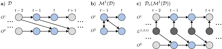
Figure 7: A ts-DAG $\mathcal{D}$ together with the ts-DMAG $\mathcal{M}^{1}(\mathcal{D})$ and the canonical ts-DAG $\mathcal{D}_{c}(\mathcal{M}^{1}(\mathcal{D}))$ of the ts-DMAG. Marginalizing $\mathcal{D}_{c}(\mathcal{M}^{1}(\mathcal{D}))$ to the observed vertices gives back $\mathcal{M}^{1}(\mathcal{D})$. Same color coding as in Fig. 2.

We stress that Lemma 4.14 holds for arbitrary ts-DAGs $\mathcal{D}$. In particular, in $\mathcal{D}$ there may be what in Malinsky and Spirtes (2018) is referred to as “auto-lag confounders”, namely unobservable autocorrelated component time series $L$, i.e., $L_{t-\tau}{\rightarrow}L_{t}$ with $L$ unobservable.

4.6 A necessary and sufficient condition that characterizes ts-DMAGs

Lemma 4.14 readily implies the following characterization of ts-DMAGs as a subclass of DMAGs with time series structure by a single necessary and sufficient condition.

Theorem 1.

Let $\mathcal{M}$ be a DMAG with time series structure and time index set $\mathbf{T}=\{t-\tau~{}|~{}0\leq t\leq p\}$. Then $\mathcal{M}$ is a ts-DMAG, i.e., there is a ts-DAG $\mathcal{D}$ such that $\mathcal{M}=\mathcal{M}^{p}(\mathcal{D})$ if and only if the MAG latent projection $\mathcal{M}^{p}(\mathcal{D}_{c}(\mathcal{M}))$ of the canonical ts-DAG $\mathcal{D}_{c}(\mathcal{M})$ of $\mathcal{M}$ equals $\mathcal{M}$, i.e., if and only if $\mathcal{M}=\mathcal{M}^{p}(\mathcal{D}_{c}(\mathcal{M}))$.

Theorem 1 is one of the central results of this paper. The following four examples are included for its illustration.

Example 4.16.

The DMAG $\mathcal{M}_{2}$ in part c) of Fig. 5 is a ts-DMAG. This conclusion follows because the canonical ts-DAG $\mathcal{D}_{c}(\mathcal{M}_{2})$ in part d) of the figure projects to $\mathcal{M}_{2}$.

Example 4.17.

One may use Theorem 1 to confirm that none of the four DMAGs in parts a) - d) of Fig. 3 is a ts-DMAG. In these cases this conclusion also follows because each of these four graphs violates at least one of the necessary conditions in Lemmas 3.7 and 4.4.

Example 4.18.

The DMAG $\mathcal{M}_{1}$ in part a) of Fig. 8 is not a ts-DMAG because its canonical ts-DAG $\mathcal{D}_{c}(\mathcal{M}_{1})$ in part b) projects to the ts-DMAG $\mathcal{M}^{1}(\mathcal{D}_{c}(\mathcal{M}_{1}))$ in part c), which is a proper subgraph of $\mathcal{M}_{1}$. This example also demonstrates that the equality $stat(\mathcal{M})=\mathcal{M}_{st}^{p}(\mathcal{D}_{c}(\mathcal{M}))$ is not sufficient for $\mathcal{M}$ to be a ts-DMAG.

Example 4.19.

The DMAG $\mathcal{M}_{2}$ in part d) of Fig. 8 is not a ts-DMAG since its canonical ts-DAG $\mathcal{D}_{c}(\mathcal{M}_{2})$ in part e) projects to the ts-DMAG $\mathcal{M}^{1}(\mathcal{D}_{c}(\mathcal{M}_{2}))$ in part f), which is a proper supergraph of $\mathcal{M}_{2}$. The edge $O^{2}_{t-1}{\leftrightarrow}O^{1}_{t}$ in $\mathcal{M}^{1}(\mathcal{D}_{c}(\mathcal{M}_{2}))$ is due to the green colored inducing path $O^{2}_{t-1}{\leftarrow}O^{2}_{t-2}{\leftarrow}O^{1}_{t-2}{\leftarrow}L^{(1,1,1)}_{t-2}{\rightarrow}O^{1}_{t-1}{\leftarrow}L^{(1,1,1)}_{t-1}{\rightarrow}O^{1}_{t}$ in $\mathcal{D}_{c}(\mathcal{M}_{2})$.

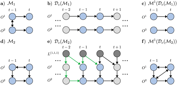
Figure 8: Two examples of DMAGs with time series structure, $\mathcal{M}_{1}$ (the same as in part part e) of Fig. 3) and $\mathcal{M}_{2}$ (the same as in part f) of Fig. 3), that are not ts-DMAGs although they obey all necessary conditions in Lemmas 3.7 and 4.4. See also the discussions in Examples 4.18 and 4.19.

Importantly, the DMAGs considered in Examples 4.18 and 4.19 obey all necessary conditions given in Lemmas 3.7 and 4.4. The condition $\mathcal{M}=\mathcal{M}^{p}(\mathcal{D}_{c}(\mathcal{M}))$ is thus strictly stronger than even the combination of all these necessary conditions. This observation clearly demonstrates the significance and non-triviality of Theorem 1.

As an alternative to Theorem 1, we also characterize ts-DMAGs as a subclass of directed mixed graphs with time series structure.

Theorem 2.

Let $\mathcal{G}$ be a directed mixed graph with time series structure and time index set $\mathbf{T}=\{t-\tau~{}|~{}0\leq t\leq p\}$. Then $\mathcal{G}$ is a ts-DMAG, i.e., there is a ts-DAG $\mathcal{D}$ such that $\mathcal{G}=\mathcal{M}^{p}(\mathcal{D})$ if and only if $\mathcal{G}$ is acyclic and $\mathcal{G}=\mathcal{M}^{p}(\mathcal{D}_{c}(\mathcal{G}))$.

Theorem 2 is even stronger than Theorem 1 because Theorem 2 does not require the graph $\mathcal{G}$ to be ancestral and/or maximal. Acyclicity, however, is needed because the definition of canonical ts-DAGs $\mathcal{D}_{c}(\mathcal{G})$ requires $\mathcal{G}$ to be acyclic, as does the notion of $d$-separation.

4.7 Implications for stationarified ts-DMAGs

A ts-DMAG $\mathcal{M}^{p}(\mathcal{D})$ by definition uniquely determines its stationarification $\mathcal{M}_{st}^{p}(\mathcal{D})$. How about the opposite? That is, can a ts-DMAG $\mathcal{M}^{p}(\mathcal{D})$ be uniquely determined from its stationarification $\mathcal{M}_{st}^{p}(\mathcal{D})$? At first it seems perfectly conceivable that different ts-DMAGs have the same stationarification, which would make it impossible to uniquely determine $\mathcal{M}_{st}^{p}(\mathcal{D})$ from $\mathcal{M}^{p}(\mathcal{D})$. However, as a corollary to the observation $\mathcal{D}_{c}(\mathcal{G})=\mathcal{D}_{c}(stat(\mathcal{G}))$ and Lemma 4.14 we get the following result.

Lemma 4.20.

Let $\mathcal{D}$ be a ts-DAG. Then, the ts-DMAG $\mathcal{M}^{p}(\mathcal{D})$ equals the MAG latent projection $\mathcal{M}^{p}(\mathcal{D}_{c}(\mathcal{M}_{st}^{p}(\mathcal{D})))$ of the canonical ts-DAG $\mathcal{D}_{c}(\mathcal{M}_{st}^{p}(\mathcal{D}))$ of the stationarification $\mathcal{M}_{st}^{p}(\mathcal{D})=stat(\mathcal{M}^{p}(\mathcal{D}))$ of $\mathcal{M}^{p}(\mathcal{D})$, i.e., $\mathcal{M}^{p}(\mathcal{D})=\mathcal{M}^{p}(\mathcal{D}_{c}(\mathcal{M}_{st}^{p}(\mathcal{D})))$.

According to Lemma 4.20 one can always uniquely determine $\mathcal{M}^{p}(\mathcal{D})$ from $\mathcal{M}_{st}^{p}(\mathcal{D})$. A ts-DMAG $\mathcal{M}^{p}(\mathcal{D})$ and its stationarification $\mathcal{M}_{st}^{p}(\mathcal{D})$ thus carry the exact same information about the underlying ts-DAG $\mathcal{D}$. In this sense $\mathcal{M}^{p}(\mathcal{D})$ and $\mathcal{M}_{st}^{p}(\mathcal{D})$ are, if interpreted in the correct way, equivalent descriptions.

Lastly, we also arrive at two characterizations of stationarified ts-DMAGs.

Lemma 4.21.

Let $\mathcal{M}$ be a DMAG with time series structure and time index set $\mathbf{T}=\{t-\tau~{}|~{}0\leq t\leq p\}$. Then, $\mathcal{M}$ is a stationarified ts-DMAG, i.e., there is a ts-DAG $\mathcal{D}$ such that $\mathcal{M}=\mathcal{M}_{st}^{p}(\mathcal{D})$ if and only if $\mathcal{M}=\mathcal{M}_{st}^{p}(\mathcal{D}_{c}(\mathcal{M}))$.

Lemma 4.22.

Let $\mathcal{G}$ be a directed mixed graph with time series structure and time index set $\mathbf{T}=\{t-\tau~{}|~{}0\leq t\leq p\}$. Then, $\mathcal{G}$ is a stationarified ts-DMAG, i.e., there is a ts-DAG $\mathcal{D}$ such that $\mathcal{G}=\mathcal{M}_{st}^{p}(\mathcal{D})$ if and only if $\mathcal{G}$ is acyclic and $\mathcal{G}=\mathcal{M}_{st}^{p}(\mathcal{D}_{c}(\mathcal{G}))$.

4.8 Comparison with previously considered model classes

The author is aware of two distinct classes of graphical models based on DMAGs that have so far been used to represent time-lag specific causal relationships in time series with latent confounders. Here, we show that both these model classes are strictly larger than the class of ts-DMAGs.

The first previously used model class, employed by the tsFCI algorithm from Entner and Hoyer (2010), are DMAGs with time series structure that are time ordered and have repeating orientations as well as past-repeating adjacencies. Lemmas 3.7 and 4.4 show that ts-DMAGs fall into this model class. The reverse, however, is not true: The graphs in part b) of Fig. 3 and parts a) and d) of Fig. 8 fall into the model class used by tsFCI but are not ts-DMAGs.

The second previously used model class, employed by the SVAR-FCI algorithm from Malinsky and Spirtes (2018) and LPCMCI from Gerhardus and Runge (2020), are DMAGs with time series structure that are time ordered and have repeating edges. From Lemma 3.7 and Def. 4.6 we see that each ts-DMAG $\mathcal{M}^{p}(\mathcal{D})$ is associated to a graph in this model, namely to the stationarified ts-DMAG $\mathcal{M}_{st}^{p}(\mathcal{D})=stat(\mathcal{M}^{p}(\mathcal{D}))$. Lemma 4.20 further implies that the mapping $\iota:\mathcal{M}^{p}(\mathcal{D})\mapsto\mathcal{M}_{st}^{p}(\mathcal{D})$ is injective. Conversely, not all graphs in the model class used by SVAR-FCI and LPCMCI are ts-DMAGs: The graph in part d) of Fig. 8 is an example.

5 Markov equivalence classes of ts-DMAGs and causal discovery

This section discusses the implications of the concepts and results of Sec. 4 for causal discovery. To this end, Def. 5.7 in Sec. 5.4 introduces time series DPAGs (ts-DPAGs) as graphs that represent Markov equivalence classes of ts-DMAGs. Time series DPAGs are refinements of DPAGs obtained by incorporating our background knowledge about the data generating process—namely that the data are generated by a process as in eq. (1) and that the observed time steps are regularly (sub-)sampled. We further introduce several alternative refinements of DPAGs, see Secs. 5.1 and 5.2, concretely DPAGs which represent Markov equivalence classes of stationarified ts-DMAGs and DPAGs which incorporate only some of the necessary properties of ts-DMAGs as background knowledge. As we show, these alternative DPAGs carry less information about the underlying ts-DAG than ts-DPAGs do. Using the introduced terminology, in Sec. 5.5 we discuss and compare three algorithms for independence-based causal discovery in time series with latent confounders and show that none of them learns ts-DPAGs. That is, all of these algorithms are conceptually suboptimal as they fail to learn causal properties of the underlying ts-DAG that in principle can be learned. As opposed to that, Algorithm 1 in Sec. 5.6 does learn ts-DPAGs and in this sense is complete. Another important result is Theorem 3 in Sec. 5.3, according to which DPAGs based on stationarified DMAGs carry less causal information than DPAGs based on non-stationarified DMAGs. Theorem 3 corrects an erroneous claim that has appeared in the literature, see the explanation below Theorem 3 in Sec. 5.3 and the discussion of the SVAR-FCI algorithm in Sec. 5.5 for more details.

5.1 Background knowledge and DPAGs

Markov equivalent DMAGs by definition have the same $m$-separations and thus cannot be distinguished by statistical independencies. They might, however, be distinguished if additional assumptions are made. One type of such assumptions is background knowledge, i.e., the assertion that DMAGs with certain properties can be excluded as these are in conflict with a priori knowledge about the system of study.

Definition 5.1 (Background knowledge, cf. Mooij and Claassen (2020)).

A background knowledge $\mathcal{A}$ is a Boolean function on the set of all DMAGs. If $\mathcal{A}(\mathcal{M})=1$, then $\mathcal{M}$ is said to be consistent with $\mathcal{A}$, else it is said to be inconsistent with $\mathcal{A}$.

Combining Definition 2 in Mooij and Claassen (2020) with the definition of PAGs in Andrews, Spirtes and Cooper (2020), we refine DPAGs by background knowledge as follows.

Definition 5.2 (DPAGs refined by background knowledge).

Let $\mathcal{M}$ be a DMAG, let $[\mathcal{M}]$ be its Markov equivalence class, and for a background knowledge $\mathcal{A}$ let $[\mathcal{M}]_{\mathcal{A}}$ be the subset of $[\mathcal{M}]$ that is consistent with $\mathcal{A}$, i.e., $[\mathcal{M}]_{\mathcal{A}}=\{\mathcal{M}\in[\mathcal{M}]~{}|~{}\mathcal{A}(\mathcal{M})=1\}$. Then:

1. A directed partial mixed graph $\mathcal{P}$ is a DPAG for $\mathcal{M}$ if

   • $\mathcal{P}$ has the same skeleton (i.e., the same set of adjacencies) as $\mathcal{M}$ and

   • every non-circle mark in $\mathcal{P}$ is also in $\mathcal{M}$.

2. A DPAG $\mathcal{P}$ for $\mathcal{M}$ is called maximally informative (m.i.) with respect to $[\mathcal{M}]^{\prime}\subseteq[\mathcal{M}]$ if

   • every non-circle mark in $\mathcal{P}$ is in every element of $[\mathcal{M}]^{\prime}$ and

   • for every circle mark in $\mathcal{P}$ there are $\mathcal{M}_{1},\mathcal{M}_{2}\in[\mathcal{M}]^{\prime}$ such that in $\mathcal{M}_{1}$ there is a tail mark and in $\mathcal{M}_{2}\in[\mathcal{M}]^{\prime}$ there is a head mark instead of the circle mark.

3. The maximally informative (m.i.) DPAG with respect to $\mathcal{A}$, denoted as $\mathcal{P}(\mathcal{M},\mathcal{A})$, is the m.i. DPAG of $\mathcal{M}$ with respect to $[\mathcal{M}]_{\mathcal{A}}$.

4. The conventional m.i. DPAG for $\mathcal{M}$ is the m.i. DPAG $\mathcal{P}(\mathcal{M})=\mathcal{P}(\mathcal{M},\mathcal{A}_{\emptyset})$, where $\mathcal{A}_{\emptyset}$ is the “empty” background knowledge for which $\mathcal{A}_{\emptyset}=1$ constant.

To compare different background knowledges and the accordingly refined DPAGs, we employ the following terminology.

Definition 5.3 (Stronger/weaker background knowledge, more/less informative DPAG).

Let $\mathcal{A}_{1}$ and $\mathcal{A}_{2}$ be background knowledges, and let $\mathcal{P}_{1}$ and $\mathcal{P}_{2}$ be DPAGs for $\mathcal{M}$. We say$\ldots$

• $\ldots$ $\mathcal{A}_{1}$ is stronger than $\mathcal{A}_{2}$ and $\mathcal{A}_{2}$ is weaker than $\mathcal{A}_{1}$ if $\mathcal{A}_{1}(\mathcal{M})=1$ implies $\mathcal{A}_{2}(\mathcal{M})=1$.

• $\ldots$ $\mathcal{P}_{1}$ is more informative than $\mathcal{P}_{2}$ and $\mathcal{P}_{2}$ is less informative than $\mathcal{P}_{1}$ if every circle mark in $\mathcal{P}_{1}$ is also in $\mathcal{P}_{2}$.

It follows that $\mathcal{P}(\mathcal{M},\mathcal{A}_{1})$ is more informative than $\mathcal{P}(\mathcal{M},\mathcal{A}_{2})$ if $\mathcal{A}_{1}$ is stronger than $\mathcal{A}_{2}$. By construction $\mathcal{P}(\mathcal{M},\mathcal{A})$ is the most informative DPAG for $\mathcal{M}$ that can be learned from statistical independencies together with the background knowledge $\mathcal{A}$.

5.2 Considered background knowledges

In the below discussions we are interested in the following background knowledges.

Definition 5.4 (Specific background knowledges).

The background knowledge of$\ldots$

• $\ldots$ an underlying ts-DAG is the background knowledge $\mathcal{A}_{\mathcal{D}}$ for which $\mathcal{A}_{\mathcal{D}}(\mathcal{M})=1$ if and only if $\mathcal{M}$ is a ts-DMAG, i.e., $\mathcal{A}_{\mathcal{D}}(\mathcal{M})=1$ if and only if there is a ts-DAG $\mathcal{D}$ with $\mathcal{M}=\mathcal{M}^{p}(\mathcal{D})$.

• $\ldots$ an underlying ts-DAG for stationarifications is the background knowledge $\mathcal{A}^{stat}_{\mathcal{D}}$ for which $\mathcal{A}^{stat}_{\mathcal{D}}(\mathcal{M})=1$ if and only if $\mathcal{M}$ is a stationarified ts-DMAG, i.e., $\mathcal{A}^{stat}_{\mathcal{D}}(\mathcal{M})=1$ if and only if there is a ts-DAG $\mathcal{D}$ with $\mathcal{M}=\mathcal{M}_{st}^{p}(\mathcal{D})$.

• $\ldots$ time order and repeating ancestral relationships is the background knowledge $\mathcal{A}_{ta}$ for which $\mathcal{A}_{ta}(\mathcal{M})=1$ if and only if $\mathcal{M}$ is time ordered and has repeating ancestral relationships.

• $\ldots$ time order and repeating orientations is the background knowledge $\mathcal{A}_{to}$ for which $\mathcal{A}_{to}(\mathcal{M})=1$ if and only if $\mathcal{M}$ is time ordered and has repeating orientations.

The first background knowledge $\mathcal{A}_{\mathcal{D}}$ is as much background knowledge as is available in the time series setting defined in Sec. 3.1. In Sec. 5.4 we will use $\mathcal{A}_{\mathcal{D}}$ to define ts-DPAGs. The second background knowledge $\mathcal{A}^{stat}_{\mathcal{D}}$ is the equivalent background knowledge when working with stationarified ts-DMAGs $\mathcal{M}_{st}^{p}(\mathcal{D})$ instead of ts-DMAGs $\mathcal{M}^{p}(\mathcal{D})$. We will use $\mathcal{A}^{stat}_{\mathcal{D}}$ to compare causal discovery based on $\mathcal{M}^{p}(\mathcal{D})$ with causal discovery based on $\mathcal{M}_{st}^{p}(\mathcal{D})$. Given that a ts-DMAG $\mathcal{M}^{p}(\mathcal{D})$ and its stationarification $\mathcal{M}_{st}^{p}(\mathcal{D})$ are in one-to-one correspondence, see Sec. 4.7, one might also expect the corresponding DPAGs to carry the same information. Interestingly, as we will show in Sec. 5.3, this expectation is incorrect. The third and fourth background knowledges $\mathcal{A}_{ta}$ and $\mathcal{A}_{to}$ equally apply to both standard and stationarified ts-DMAGs. They are included for comparison with existing causal discovery algorithms.

The four specified background knowledges compare as follows: Since both ts-DMAGs $\mathcal{M}^{p}(\mathcal{D})$ and stationarified ts-DMAGs $\mathcal{M}_{st}^{p}(\mathcal{D})$ are time ordered and have repeating ancestral relationships, both $\mathcal{A}_{\mathcal{D}}$ and $\mathcal{A}^{stat}_{\mathcal{D}}$ are stronger than $\mathcal{A}_{ta}$. Since repeating ancestral relationships imply repeating orientations, $\mathcal{A}_{ta}$ is stronger than $\mathcal{A}_{to}$. For stationarified ts-DMAGs $\mathcal{M}_{st}^{p}(\mathcal{D})$, however, $\mathcal{A}_{ta}$ and $\mathcal{A}_{to}$ are equivalent (as follows from Lemma 4.3). In our notation this equivalence is expressed as $\mathcal{P}(\mathcal{M}_{st}^{p}(\mathcal{D}),\mathcal{A}_{ta})=\mathcal{P}(\mathcal{M}_{st}^{p}(\mathcal{D}),\mathcal{A}_{to})$.

5.3 DPAGs of ts-DMAGs $\mathcal{M}^{p}(\mathcal{D})$ carry more information than DPAGs of stationarified ts-DMAGs $\mathcal{M}_{st}^{p}(\mathcal{D})$

In this subsection we show that, when working with the background knowledges specified in Def. 5.4, DPAGs of ts-DMAGs can never carry less but may carry more information about the underlying ts-DAG than DPAGs of stationarified ts-DMAGs. This is so despite the fact that, as explained in Sec. 4.7, a ts-DMAG and its stationarification are in one-to-one correspondence. Towards proving the claim we first note the following.

Lemma 5.5.

Let $\mathcal{D}$ be a ts-DAG and let $\mathcal{A}\in\{\mathcal{A}_{\mathcal{D}},\mathcal{A}_{ta},\mathcal{A}_{to}\}$. Then, the graph $stat(\mathcal{P}(\mathcal{M}^{p}(\mathcal{D}),\mathcal{A}))$ is a DPAG for $\mathcal{M}_{st}^{p}(\mathcal{D})$.

In particular, both DPAGs $\mathcal{P}(\mathcal{M}_{st}^{p}(\mathcal{D}),\mathcal{A}^{stat})$ and $stat(\mathcal{P}(\mathcal{M}^{p}(\mathcal{D}),\mathcal{A}))$ have the same adjacencies. Moreover, it is well-defined to ask whether one of the two DPAGs is more informative than the other. The following result answers this question.

Theorem 3.

Let $\mathcal{D}$ be a ts-DAG and let $(\mathcal{A},\mathcal{A}^{stat})$ either be $(\mathcal{A}_{to},\mathcal{A}_{to})$ or $(\mathcal{A}_{ta},\mathcal{A}_{ta})$ or $(\mathcal{A}_{\mathcal{D}},\mathcal{A}^{stat}_{\mathcal{D}})$. Then:

1. Every non-circle mark (head or tail) in $\mathcal{P}(\mathcal{M}_{st}^{p}(\mathcal{D}),\mathcal{A}^{stat})$ is also in $stat(\mathcal{P}(\mathcal{M}^{p}(\mathcal{D}),\mathcal{A}))$.

2. Every non-circle mark in $\mathcal{P}(\mathcal{M}_{st}^{p}(\mathcal{D}),\mathcal{A}^{stat})$ is also in $\mathcal{P}(\mathcal{M}^{p}(\mathcal{D}),\mathcal{A})$.

3. There are cases in which a non-circle mark that is in $stat(\mathcal{P}(\mathcal{M}^{p}(\mathcal{D}),\mathcal{A}))$ is not also in $\mathcal{P}(\mathcal{M}_{st}^{p}(\mathcal{D}),\mathcal{A}^{stat})$.

4. There are cases in which a non-circle mark that is in $\mathcal{P}(\mathcal{M}^{p}(\mathcal{D}),\mathcal{A})$ is not also in $\mathcal{P}(\mathcal{M}_{st}^{p}(\mathcal{D}),\mathcal{A}^{stat})$, even regarding adjacencies that are shared by both graphs.

Theorem 3 contradicts the opposite claim in Malinsky and Spirtes (2018) according to which more unambiguous edge orientations (heads or tails) may be inferred if, as licensed by the assumption of causal stationarity, the property of repeating adjacencies is enforced in causal discovery; see Sec. 5.5 for more details. The following example illustrates Theorem 3.

Example 5.6.

Part a) and b) of Fig. 9 respectively show a ts-DMAG $\mathcal{M}^{p}(\mathcal{D})$ and its conventional m.i. DPAG $\mathcal{P}(\mathcal{M}^{p}(\mathcal{D}))$. To derive $\mathcal{P}(\mathcal{M}^{p}(\mathcal{D}))$ one may, for example, apply the FCI orientation rules, see Zhang (2008b), to the skeleton of $\mathcal{M}^{p}(\mathcal{D})$. Part c) of the same figure shows $\mathcal{P}(\mathcal{M}^{p}(\mathcal{D}),\mathcal{A}_{to})$, where the head at $O^{2}_{t}$ on $O^{2}_{t-1}{\leftrightarrow}O^{2}_{t}$ follows by time order. Repeating orientations does not help in orienting the last remaining circle mark on $O^{1}_{t-1}{\circ\!{\rightarrow}}O^{2}_{t-1}$ because $O^{1}_{t}$ and $O^{2}_{t}$ are non-adjacent. The stronger background knowledge $\mathcal{A}_{ta}$ is, however, sufficient to do so: Vertex $O^{1}_{t-1}$ cannot be an ancestor of $O^{2}_{t-1}$ because $O^{1}_{t}$ is not an ancestor of $O^{2}_{t}$, which in turn follows because there is no possibly directed path from $O^{1}_{t}$ to $O^{2}_{t}$, see Zhang (2006, pp. 81f). We hence get the DPAG $\mathcal{P}(\mathcal{M}^{p}(\mathcal{D}),\mathcal{A}_{ta})$ shown in part d). Since there are no circle marks left, $\mathcal{P}(\mathcal{M}^{p}(\mathcal{D}),\mathcal{A}_{ta})$ here equals the DPAG $\mathcal{P}(\mathcal{M}^{p}(\mathcal{D}),\mathcal{A}_{\mathcal{D}})$ in part e). The graphs $stat(\mathcal{P}(\mathcal{M}^{p}(\mathcal{D}),\mathcal{A}_{to}))$, $stat(\mathcal{P}(\mathcal{M}^{p}(\mathcal{D}),\mathcal{A}_{ta}))$ and $stat(\mathcal{P}(\mathcal{M}^{p}(\mathcal{D}),\mathcal{A}_{\mathcal{D}}))$ are respectively obtained by removing the edge between $O^{1}_{t-1}$ and $O^{2}_{t-2}$ from the graphs in parts c), d) and e). The stationarified ts-DMAG $\mathcal{M}_{st}^{p}(\mathcal{D})$ and its conventional m.i. DPAG $\mathcal{P}(\mathcal{M}_{st}^{p}(\mathcal{D}))$ are shown in part f) and g). Part h) shows $\mathcal{P}(\mathcal{M}_{st}^{p}(\mathcal{D}),\mathcal{A}_{to})$, where there is a head mark at $O^{2}_{t}$ on $O^{2}_{t-1}{\rightarrow}O^{2}_{t}$ due to time order. As explained in Sec. 5.2, the equality $\mathcal{P}(\mathcal{M}_{st}^{p}(\mathcal{D}),\mathcal{A}_{to})=\mathcal{P}(\mathcal{M}_{st}^{p}(\mathcal{D}),\mathcal{A}_{ta})$ always holds. With the characterization of stationarified ts-DMAGs in Lemma 4.21 (or Lemma 4.22) we can further show that in this example the graph in h) equals $\mathcal{P}(\mathcal{M}_{st}^{p}(\mathcal{D}),\mathcal{A}_{\mathcal{D}})$ in part i). Note that the ts-DMAG $\mathcal{M}^{1}(\mathcal{D})$ in part a) is indeed a ts-DMAG. For example, its canonical ts-DAG $\mathcal{D}_{c}(\mathcal{M}^{1}(\mathcal{D}))$ projects to $\mathcal{M}^{1}(\mathcal{D})$.

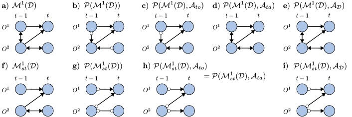
Figure 9: An example for illustrating Theorem 3, see also the discussion in Example 5.6.

Theorem 3 and Example 5.6 show that $\mathcal{P}(\mathcal{M}^{p}(\mathcal{D}),\mathcal{A})$ and $stat(\mathcal{P}(\mathcal{M}^{p}(\mathcal{D}),\mathcal{A}))$ have more unambiguous edge marks than $\mathcal{P}(\mathcal{M}_{st}^{p}(\mathcal{D}),\mathcal{A}^{stat})$. It thus is conceptually advantageous to work with DPAGs $\mathcal{P}(\mathcal{M}^{p}(\mathcal{D}),\mathcal{A})$ of ts-DMAGs—or with their stationarifications $stat(\mathcal{P}(\mathcal{M}^{p}(\mathcal{D}),\mathcal{A}))$, if one prefers graphs with repeating edges—rather than with DPAGs $\mathcal{P}(\mathcal{M}_{st}^{p}(\mathcal{D}),\mathcal{A}^{stat})$ of stationarified ts-DMAGs. One might argue, though, that the additional ambiguous orientations (i.e., circle marks) which $\mathcal{P}(\mathcal{M}_{st}^{p}(\mathcal{D}),\mathcal{A}^{stat})$ has as compared to $\mathcal{P}(\mathcal{M}^{p}(\mathcal{D}),\mathcal{A})$ might turn into unambiguous orientations (i.e., head or tail marks) in $\mathcal{P}(\mathcal{M}^{\tilde{p}}_{st}(\mathcal{D}),\mathcal{A}^{stat})$ for an increased length $\tilde{p}>p$ of the observed time window. However, increasing $p$ to $\tilde{p}$ also increases the number of observed vertices and thus yields a higher-dimensional causal discovery problem. Having more observed vertices typically hurts finite-sample performance of causal discovery, see, e.g., the simulation studies in Gerhardus and Runge (2020). On the other hand, algorithms that work with stationarified ts-DMAGs rather than ts-DMAGs may scale more favorably with the length $p$ of the observed time window because they remove the edges $O^{i}_{t-\Delta t-\tau}{\ast\!{\--}\!\ast}O^{j}_{t-\Delta t}$ for all $\Delta t$ as soon as the edge $O^{i}_{t-\tau}{\ast\!{\--}\!\ast}O^{j}_{t}$ is removed and therefore typically make fewer independence tests. From a practical perspective there thus is a trade-off between working with ts-DMAGs vs. working with stationarified ts-DMAGs, which calls for empirical evaluation in future work.

5.4 Time series DPAGs

In Sec. 5.3 we showed that DPAGs of ts-DMAGs always carry more information about the underlying ts-DAG than DPAGs of stationarified ts-DMAGs. Because of this fact we choose to define time series DPAGs as the former type of DPAGs.

Definition 5.7 (Time series DPAG).

Let $\mathcal{D}$ be a ts-DAG with variable index set $\mathbf{I}$, let $\mathbf{I}_{\mathbf{O}}\subseteq\mathbf{I}$, and let $\mathbf{T}_{\mathbf{O}}\subsetneq\mathbb{Z}$ be regularly sampled or regularly subsampled. The time series DPAG implied by $\mathcal{D}$ over $\mathbf{O}=\mathbf{I}_{\mathbf{O}}\times\mathbf{T}_{\mathbf{O}}$, denoted as $\mathcal{P}_{\mathbf{O}}(\mathcal{D})$ or $\mathcal{P}_{\mathbf{I}_{\mathbf{O}}\times\mathbf{T}_{\mathbf{O}}}(\mathcal{D})$ and also referred to as a ts-DPAG, is the m.i. DPAG $\mathcal{P}(\mathcal{M}_{\mathbf{O}}(\mathcal{D}),\mathcal{A}_{\mathcal{D}})$.

Remark (on Def. 5.7).

The equivalence of regular sampling and regular subsampling, see Sec. 4.2, carries over to ts-DPAGs. We hence restrict to regular sampling without loss of generality and write $\mathcal{P}^{p}(\mathcal{D})$ for $\mathcal{P}_{\mathbf{O}}(\mathcal{D})$ with $\mathbf{O}=\mathbf{I}_{\mathbf{O}}\times\mathbf{T}_{\mathbf{O}}$ and $\mathbf{T}_{\mathbf{O}}=\{t-\tau~{}|~{}0\leq\tau\leq p\}$.

The following example discusses a case in which the use of the strongest background knowledge $\mathcal{A}_{\mathcal{D}}$ leads to strictly more unambiguous edge orientations than $\mathcal{A}_{ta}$. We thus cannot replace $\mathcal{A}_{\mathcal{D}}$ with $\mathcal{A}_{ta}$ in the definition of ts-DPAGs without losing information.

Example 5.8.

The ts-DMAG $\mathcal{M}^{1}(\mathcal{D})$ in part a) of Fig. 10 gives rise to $\mathcal{P}(\mathcal{M}^{1}(\mathcal{D}),\mathcal{A}_{ta})$ in part b) with a circle mark at $O^{1}_{t}$ on $O^{1}_{t-1}{\circ\!{\rightarrow}}O^{1}_{t}$. According to the stronger background knowledge $\mathcal{A}_{\mathcal{D}}$ one can orient this edge as $O^{1}_{t-1}{\rightarrow}O^{1}_{t}$ because the opposite hypothesis gives the graph in part d) in Fig. 8, which by means of Theorem 1 was shown to not be a ts-DMAG, see Example 4.19. Thus, from the ts-DPAG $\mathcal{P}^{1}(\mathcal{D})$ we can conclude that $O^{1}_{t-1}$ has a causal influence on $O^{1}_{t}$ whereas from $\mathcal{P}(\mathcal{M}^{1}(\mathcal{D}),\mathcal{A}_{ta})$ we can only conclude that this causal influence might but also might not exist.

Furthermore, see Gerhardus (2023, Lemma B.8), in the ts-DMAG $\mathcal{M}^{1}(\mathcal{D})$ the pair $(O^{1}_{t-1},O^{1}_{t})$ cannot suffer from latent confounding. Thus, the causal effect of $O^{1}_{t-1}$ on $O^{1}_{t}$ is identifiable and can be estimated from observations by adjusting for the empty set. Importantly, if we interpret $\mathcal{M}^{1}(\mathcal{D})$ not as a ts-DMAG but as a “standard” DMAG, then the causal effect of $O^{1}_{t-1}$ on $O^{1}_{t}$ would be unidentifiable as follows from Lemma 10 in Zhang (2008a).

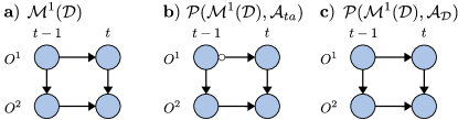
Figure 10: A case in which $\mathcal{P}^{p}(\mathcal{D})$ has a non-circle mark that is not in $\mathcal{P}(\mathcal{M}^{p}(\mathcal{D}),\mathcal{A}_{ta})$.

Example 5.8 clearly demonstrates the importance of our characterization of ts-DMAGs for the tasks of causal discovery and causal inference. Moreover, the following result shows that ts-DPAGs are complete with respect to ancestral relationships.

Lemma 5.9.

If in a ts-DPAG $\mathcal{P}^{p}(\mathcal{D})$ there is an edge $(i,t_{i}){\circ\!{\--}}\!\!\!\ast(j,t_{j})$, then there are ts-DAGs $\mathcal{D}_{1}$ and $\mathcal{D}_{2}$ such that both ts-DMAGs $\mathcal{M}^{p}(\mathcal{D}_{1})$ and $\mathcal{M}^{p}(\mathcal{D}_{2})$ are Markov equivalent to the ts-DMAG $\mathcal{M}^{p}(\mathcal{D})$ and $(i,t_{i})\in an((j,t_{j}),\mathcal{D}_{1})$ and $(i,t_{i})\notin an((j,t_{j}),\mathcal{D}_{2})$.

5.5 Existing causal discovery algorithms do not learn ts-DPAGs

To the best of the author’s knowledge, so far there is no causal discovery algorithm that learns ts-DPAGs $\mathcal{P}^{p}(\mathcal{D})$. Hence, all existing causal discovery algorithms fail to learn some causal relationships that can be learned. This failure also applies to the independence-based algorithms tsFCI from Entner and Hoyer (2010), SVAR-FCI from Malinsky and Spirtes (2018) and LPCMCI from Gerhardus and Runge (2020). Below, we discuss and compare these three algorithms conceptually (but also note the practical considerations discussed at the end of Sec. 5.3).

The tsFCI algorithm from Entner and Hoyer (2010) refines the well-known FCI algorithm, see Spirtes, Meek and Richardson (1995), Spirtes, Glymour and Scheines (2000), Zhang (2008b), to structural processes as in eq. (1). To this end, see the blue colored instructions in parts 2(a) and 2(b) of Algorithm 1 in Entner and Hoyer (2010), tsFCI imposes time order from the start and enforces repeating orientations at all steps. In addition, see the blue colored instructions in parts 1(b) and 1(c) of Algorithm 1 in Entner and Hoyer (2010), tsFCI excludes future vertices from conditioning sets and uses repeating separating sets to avoid unnecessary independence tests (these latter two modifications are, however, only relevant computationally and statistically but not conceptually). Importantly, Entner and Hoyer (2010) introduces two variants of the algorithm. The first variant, which we call tsFCI^l (with ‘$l$’ for ‘lagged’), assumes that in the data-generating ts-DAG there are no contemporaneous edges and hence orients all contemporaneous edges in the DPAG as bidirected. This first variant is as specified by Algorithm 1 in Entner and Hoyer (2010). However, in section 6 of Entner and Hoyer (2010) (see, in particular, their footnote 3) the authors explain the minor modifications that have to be done when not making the additional assumption of no contemporaneous causation. Moreover, there they also show an application of the resulting more general variant. We refer to this second variant as tsFCI^l+c (with ‘$l+c$’ for ‘lagged plus contemporaneous’). To summarize, in our terminology tsFCI^l+c attempts to learn the DPAG $\mathcal{P}(\mathcal{M}^{p}(\mathcal{D}),\mathcal{A}_{to})$ of the ts-DMAG $\mathcal{M}^{p}(\mathcal{D})$. Since $\mathcal{P}(\mathcal{M}^{p}(\mathcal{D}),\mathcal{A}_{to})$ may contain circle marks that are not in the ts-DPAG $\mathcal{P}^{p}(\mathcal{D})=\mathcal{P}(\mathcal{M}^{p}(\mathcal{D}),\mathcal{A}_{\mathcal{D}})$, see Examples 5.6 and 5.8, tsFCI^l+c does not learn all ancestral relationships that can be learned when using the available background knowledge $\mathcal{A}_{\mathcal{D}}$. From Example 5.6 we even conclude that tsFCI^l+c learns fewer orientations as can be learned with the weaker background knowledge $\mathcal{A}_{ta}$.

As compared to tsFCI^l+c, the more recent SVAR-FCI algorithm from Malinsky and Spirtes (2018) enforces repeating adjacencies by removing the edges $O^{i}_{t-\Delta t-\tau}{\ast\!{\--}\!\ast}O^{j}_{t-\Delta t}$ for all $\Delta t$ as soon as the edge $O^{i}_{t-\tau}{\ast\!{\--}\!\ast}O^{j}_{t}$ is removed—even in cases where there is no associated separating set in the observed time window. This modification is achieved by the respective second lines in the “then”-clauses in steps 5 and 11 of Algorithm 3.1 in Malinsky and Spirtes (2018). Consequently, SVAR-FCI finds a skeleton which has repeating adjacencies, i.e., SVAR-FCI finds the skeleton of the stationarified ts-DMAG $\mathcal{M}_{st}^{p}(\mathcal{D})$ rather than the skeleton of the ts-DMAG $\mathcal{M}^{p}(\mathcal{D})$. On the skeleton of $\mathcal{M}_{st}^{p}(\mathcal{D})$ the algorithm then applies the FCI orientation rules, augmented with the background knowledge of time order and repeating orientations. In our terminology SVAR-FCI hence attempts to learn the DPAG $\mathcal{P}(\mathcal{M}_{st}^{p}(\mathcal{D}),\mathcal{A}_{to})$ of the stationarified ts-DMAG $\mathcal{M}_{st}^{p}(\mathcal{D})$. Now recall Theorem 3, which says that all unambiguous edge orientations in this DPAG $\mathcal{P}(\mathcal{M}_{st}^{p}(\mathcal{D}),\mathcal{A}_{to})$ are also in $\mathcal{P}(\mathcal{M}^{p}(\mathcal{D}),\mathcal{A}_{to})$—the one learned by tsFCI^l+c—while there are cases in which the opposite is not true. Thus, if ground-truth knowledge of (conditional) independencies is given, SVAR-FCI can never learn more unambiguous edge orientations than tsFCI^l+c while there are cases in which it learns strictly fewer. The additional edge removals thus actually have the opposite effect of what was intended in Malinsky and Spirtes (2018). Moreover, also SVAR-FCI fails to learn all identifiable ancestral relationships of the underlying ts-DAG.

Example 5.10.

Assume ground-truth knowledge about (conditional) independencies. When applied to the ts-DMAG in part a) of Fig. 9, tsFCI^l+c returns the graph in part c) whereas SVAR-FCI returns the graph in part h) with strictly fewer unambiguous edge marks. This difference is relevant: From tsFCI^l+c’s output we can conclude that $O^{2}_{t-1}$ generically has a causal effect on $O^{1}_{t}$ whereas from SVAR-FCI’s output we can only conclude that $O^{2}_{t-1}$ might but also might not generically have a causal effect on $O^{1}_{t}$. As another difference, tsFCI^l+c gives the edge $O^{1}_{t-1}{\circ\!{\rightarrow}}O^{2}_{t-1}$ whereas SVAR-FCI gives that $O^{1}_{t-1}$ and $O^{2}_{t-1}$ are non-adjacent. At first one might think that SVAR-FCI is at the advantage in this regard, because the absence of an edge between $O^{1}_{t-1}$ and $O^{2}_{t-1}$ correctly conveys that the pair $(O^{1}_{t-1},O^{2}_{t-1})$ is not confounded by unobservable variables. Note, however, that tsFCI^l+c conveys the same conclusion by means of having learned that $O^{1}_{t}$ and $O^{2}_{t}$ are non-adjacent (cf. last paragraph in Sec. 4.4). In fact, see Theorem 3, one can always post-process the output of tsFCI^l+c by stationarification $stat(\cdot)$ to obtain a graph that, compared to the graph learned by SVAR-FCI, has the same adjacencies and the same or more unambiguous edge orientations. In the current example, this post-processing step amounts to removing the edge $O^{1}_{t-1}{\circ\!{\rightarrow}}O^{2}_{t-1}$ from the graph in part c) of Fig. 9.

The LPCMCI algorithm from Gerhardus and Runge (2020) applies several modifications to SVAR-FCI that significantly improve the finite-sample performance. The infinite sample properties are unchanged, however. Thus also LPCMCI in general learns fewer orientations than tsFCI^l+c and fails to learn all ancestral relationships that can be learned.

5.6 ts-DPAGs can be learned from data

In this subsection we show that ts-DPAGs can, at least in principle, be learned from data. In fact, using the characterization of ts-DMAGs by Theorem 1, we can immediately write down Algorithm 1 for this purpose.

Practically, however, finding the set of candidate DMAGs $\mathbf{M}^{\ast}$ in step 2 is expected to become computationally infeasible for large graphs $\mathcal{P}^{\ast}$. This expectation is based on the empirical finding in Malinsky and Spirtes (2016) according to which the Zhang MAG listing algorithm (there used not for causal discovery but for causal effect estimation and in a non-temporal setting) becomes too slow for graphs with about $15$ to $20$ vertices. On the contrary, when using tsFCI^l+c in step 1, the DPAG $\mathcal{P}^{\ast}$ already incorporates the background knowledge $\mathcal{A}_{to}$ of time order and repeating orientations. Hence, $\mathcal{P}^{\ast}$ will tend to have fewer circle marks than a typical DPAG in the non-temporal setting. Therefore, Algorithm 1 might be feasible for yet larger graphs. Nevertheless, it would be desirable to instead derive orientation rules that impose the background knowledge $\mathcal{A}_{\mathcal{D}}$ directly on $\mathcal{P}^{\ast}$ and thus entirely circumvent the need to determine the set $\mathbf{M}^{\ast}$. Moreover, recalling from the remark on Def. 3.6, an implementation of the projection procedure required for step 3 is possible but non-trivial and will be left to future work, see Gerhardus et al. (2023). The following example illustrates Algorithm 1.

Algorithm 1 Learning ts-DPAGs

1:Apply any causal discovery algorithm on the time window $[t-p,t]$ that determines a DPAG $\mathcal{P}^{\ast}$ for $\mathcal{M}^{p}(\mathcal{D})$ which is at least as informative as the conventional m.i. DPAG $\mathcal{P}(\mathcal{M}^{p}(\mathcal{D}))$. The tsFCI^l+c algorithm meets this requirement, whereas SVAR-FCI and LPCMCI do not meet this requirement.

2:Let $\mathbf{M}^{\ast}$ be the set of all DMAGs that are represented by and are Markov equivalent to the DPAG $\mathcal{P}^{\ast}$. This step can, e.g., be done with the Zhang MAG listing algorithm described in Malinsky and Spirtes (2016).

3:Let $\mathbf{M}$ be the set of all DMAGs $\mathcal{M}\in\mathbf{M}^{\ast}$ for which $\mathcal{M}=\mathcal{M}^{p}(\mathcal{D}_{c}(\mathcal{M}))$. This step can be executed as follows: For each $\mathcal{M}\in\mathbf{M}^{\ast}$, first, construct the canonical ts-DAG $\mathcal{D}_{c}(\mathcal{M})$ by applying Def. 4.13 and, second, apply the MAG latent projection to determine the ts-DMAG $\mathcal{M}^{p}(\mathcal{D}_{c}(\mathcal{M}))$ and, third, check for equality of the graphs $\mathcal{M}$ and $\mathcal{M}^{p}(\mathcal{D}_{c}(\mathcal{M}))$.

4:Let $\mathcal{P}$ be the m.i. DPAG with respect to the set $\mathbf{M}$. Note that parts 1 and 2 of Def. 5.2 specify how $\mathcal{P}$ is determined from $\mathbf{M}$.

5:return ts-DPAG $\mathcal{P}=\mathcal{P}^{p}(\mathcal{D})$

Example 5.11.

Consider the graph $\mathcal{P}(\mathcal{M}^{1}(\mathcal{D}),\mathcal{A}_{ta})$ in part b) of Fig. 10, which in this example equals $\mathcal{P}(\mathcal{M}^{1}(\mathcal{D}),\mathcal{A}_{to})$. Given ground-truth knowledge of (conditional) independencies, this graph is the output of tsFCI^l+c (and of SVAR-FCI and LPCMCI) on any ts-DAG $\mathcal{D}$ that projects to $\mathcal{M}^{1}(\mathcal{D})$ in part a) of the figure. Such $\mathcal{D}$ exists, e.g. the canonical ts-DAG $\mathcal{D}_{c}(\mathcal{M}^{1}(\mathcal{D}))$ of $\mathcal{M}^{1}(\mathcal{D})$. There is exactly one circle mark in $\mathcal{P}^{\ast}=\mathcal{P}(\mathcal{M}^{1}(\mathcal{D}),\mathcal{A}_{ta})$, namely on $O^{1}_{t-1}{\circ\!{\rightarrow}}O^{1}_{t}$. This circle mark can be oriented either as a tail ($O^{1}_{t-1}{\rightarrow}O^{1}_{t}$), giving rise to a DMAG $\mathcal{M}_{1}$, or as a head ($O^{1}_{t-1}{\leftrightarrow}O^{1}_{t}$), giving rise to a DMAG $\mathcal{M}_{2}$. Both of these candidates are represented by and Markov equivalent to $\mathcal{P}^{\ast}$, hence $\mathbf{M}^{\ast}=\{\mathcal{M}_{1},\mathcal{M}_{2}\}$. Moving to step 3, the first candidate $\mathcal{M}_{1}$ passes the check $\mathcal{M}_{1}=\mathcal{M}^{1}(\mathcal{D}_{c}(\mathcal{M}_{1}))$, whereas (see Example 5.8) $\mathcal{M}_{2}\neq\mathcal{M}^{1}(\mathcal{D}_{c}(\mathcal{M}_{2}))$ for the second candidate $\mathcal{M}_{2}$. Thus $\mathbf{M}=\{\mathcal{M}_{1}\}$. Since there is only a single element $\mathcal{M}_{1}$ in $\mathbf{M}$, this DMAG $\mathcal{M}_{1}$ according to parts 1 and 2 of Def. 5.2 equals the ts-DPAG $\mathcal{P}^{1}(\mathcal{D})$. Noting that $\mathcal{P}^{1}(\mathcal{D})$ (learned by Algorithm 1) has an additional unambiguous edge mark as compared to $\mathcal{P}(\mathcal{M}^{1}(\mathcal{D}),\mathcal{A}_{to})$ (learned by tsFCI^l+c, SVAR-FCI and LPCMCI), we see that Algorithm 1 is indeed more informative than the existing algorithms.

Remark (on Example 5.11).

The example has two non-generic properties. First, see Gerhardus (2023, Fig. C and Example B.15), in general there can be circle marks in the ts-DPAG $\mathcal{P}^{p}(\mathcal{D})$. Second, the ts-DMAG $\mathcal{M}^{p}(\mathcal{D})=\mathcal{M}^{1}(\mathcal{D})$ here has repeating edges and thus equals $\mathcal{M}_{st}^{p}(\mathcal{D})=\mathcal{M}^{1}_{st}(\mathcal{D})$. Only if the equality $\mathcal{M}^{p}(\mathcal{D})=\mathcal{M}_{st}^{p}(\mathcal{D})$ holds, then also SVAR-FCI and LPCMCI learn the DPAG $\mathcal{P}^{\ast}=\mathcal{P}(\mathcal{M}^{p}(\mathcal{D}),\mathcal{A}_{to})$, which then also necessarily equals $\mathcal{P}(\mathcal{M}^{p}(\mathcal{D}),\mathcal{A}_{ta})$. In general, however, $\mathcal{M}^{p}(\mathcal{D})$ and $\mathcal{M}_{st}^{p}(\mathcal{D})$ are not equal and neither SVAR-FCI nor LPCMCI may be used for step 1 of Algorithm 1, see Fig. 9 and Example 5.6.

6 Discussion

In this paper, we developed and analyzed ts-DMAGs, a class of graphical models for representing time-lag specific causal relationships and independencies among finitely many regularly (sub-)sampled time steps of causally stationary multivariate time series with unobserved components. As a central result, Theorems 1 and 2 completely characterize ts-DMAGs. Examples demonstrated that ts-DMAGs constitute a strictly smaller class of graphical models than the graphs that have previously been employed in the literature, see Sec. 4.8 for details. At the same time, using ts-DMAGs does not require additional assumptions or restrictions on the data-generating process. From ts-DMAGs one can thus draw stronger causal inferences than from the previously employed model classes, both in causal discovery and causal effect estimation. In addition, we defined ts-DPAGs as representations of Markov equivalence classes of ts-DMAGs. Time series DPAGs contain as much information about the ancestral relationships as can in principle be learned from observational data under the standard assumptions of independence-based causal discovery. We then showed that current time series causal discovery algorithms do not learn ts-DPAGs, i.e., they fail to learn some causal relationships that can be learned. As opposed to that, Algorithm 1 does learn ts-DPAGs. With Theorem 3 we corrected the incorrect claim from the literature that causal discovery on stationarified DMAGs gives more unambiguous edge orientations than causal discovery on non-stationarified DMAGs—in fact, the opposite is true. We envision that these results will be used to improve time series causal inference methods that resolve time lags, which in turn can have applications in diverse scientific and technical domains.

The results presented here point to various directions of future research. First, it would be valuable to consider the causal discovery problem in more detail. In particular, it is desirable to develop orientation rules that impose the background knowledge of an underlying ts-DAG $\mathcal{A}_{\mathcal{D}}$ without the need for listing all DMAGs consistent with $\mathcal{A}_{\mathcal{D}}$. Second, it remains open to characterize the causal inferences that can be drawn from ts-DMAGs and ts-DPAGs. As shown by Example 5.8, deriving such a characterization is a non-trivial task that goes beyond the corresponding task in the non-temporal setting. Third, one may analyze the additional restrictions and causal inferences that follow when, as opposed to this work, assumptions on the connectivity pattern of the underlying ts-DAG are imposed. Lastly, it is desirable to generalize our results to cases with cyclic causal relationships and selection variables.

[Acknowledgments] I thank Jakob Runge for helpful discussions and suggestions. I thank Tom Hochsprung and Wiebke Günther for careful proofreading and suggestions on how to make the paper more accessible. I thank two anonymous reviewers and two anonymous Associate Editors for suggestions and questions that helped me to improve the paper.

Supplement to “Characterization of causal ancestral graphs for time series with latent confounders” This Supplementary Material contains: First, a glossary of abbreviations and frequently used symbols. Second, theoretical results that were omitted from the main text due to space constraints. Third, proofs of all theoretical results presented in the main text together with various auxiliary results that are used in these proofs.

References

- Ali, Richardson and Spirtes (2009) {barticle}[author] \bauthor\bsnmAli, \bfnmR. Ayesha\binitsR. A., \bauthor\bsnmRichardson, \bfnmThomas S.\binitsT. S. and \bauthor\bsnmSpirtes, \bfnmPeter\binitsP. (\byear2009). \btitleMarkov Equivalence for Ancestral Graphs. \bjournalThe Annals of Statistics \bvolume37 \bpages2808–2837. \endbibitem
- Andrews, Spirtes and Cooper (2020) {binproceedings}[author] \bauthor\bsnmAndrews, \bfnmBryan\binitsB., \bauthor\bsnmSpirtes, \bfnmPeter\binitsP. and \bauthor\bsnmCooper, \bfnmGregory F.\binitsG. F. (\byear2020). \btitleOn the Completeness of Causal Discovery in the Presence of Latent Confounding with Tiered Background Knowledge. In \bbooktitleProceedings of the Twenty Third International Conference on Artificial Intelligence and Statistics (\beditor\bfnmSilvia\binitsS. \bsnmChiappa and \beditor\bfnmRoberto\binitsR. \bsnmCalandra, eds.). \bseriesProceedings of Machine Learning Research \bvolume108 \bpages4002–4011. \bpublisherPMLR. \endbibitem
- Assaad, Devijver and Gaussier (2022) {binproceedings}[author] \bauthor\bsnmAssaad, \bfnmCharles K.\binitsC. K., \bauthor\bsnmDevijver, \bfnmEmilie\binitsE. and \bauthor\bsnmGaussier, \bfnmEric\binitsE. (\byear2022). \btitleDiscovery of extended summary graphs in time series. In \bbooktitleProceedings of the Thirty-Eighth Conference on Uncertainty in Artificial Intelligence (\beditor\bfnmJames\binitsJ. \bsnmCussens and \beditor\bfnmKun\binitsK. \bsnmZhang, eds.). \bseriesProceedings of Machine Learning Research \bvolume180 \bpages96–106. \bpublisherPMLR. \endbibitem
- Bollen (1989) {bbook}[author] \bauthor\bsnmBollen, \bfnmKenneth A\binitsK. A. (\byear1989). \btitleStructural Equations with Latent Variables. \bpublisherJohn Wiley & Sons, \baddressNew York, NY, USA. \endbibitem
- Bongers, Blom and Mooij (2018) {barticle}[author] \bauthor\bsnmBongers, \bfnmStephan\binitsS., \bauthor\bsnmBlom, \bfnmTineke\binitsT. and \bauthor\bsnmMooij, \bfnmJoris M\binitsJ. M. (\byear2018). \btitleCausal modeling of dynamical systems. \bjournalarXiv preprint arXiv:1803.08784. \endbibitem
- Chu and Glymour (2008) {barticle}[author] \bauthor\bsnmChu, \bfnmTianjiao\binitsT. and \bauthor\bsnmGlymour, \bfnmClark\binitsC. (\byear2008). \btitleSearch for Additive Nonlinear Time Series Causal Models. \bjournalJournal of Machine Learning Research \bvolume9 \bpages967–991. \endbibitem
- Didelez (2008) {barticle}[author] \bauthor\bsnmDidelez, \bfnmVanessa\binitsV. (\byear2008). \btitleGraphical models for marked point processes based on local independence. \bjournalJournal of the Royal Statistical Society: Series B (Statistical Methodology) \bvolume70 \bpages245–264. \endbibitem
- Eichler (2010) {binproceedings}[author] \bauthor\bsnmEichler, \bfnmMichael\binitsM. (\byear2010). \btitleGraphical Gaussian modelling of multivariate time series with latent variables. In \bbooktitleProceedings of the Thirteenth International Conference on Artificial Intelligence and Statistics \bpages193–200. \bpublisherJMLR Workshop and Conference Proceedings. \endbibitem
- Eichler and Didelez (2007) {binproceedings}[author] \bauthor\bsnmEichler, \bfnmMichael\binitsM. and \bauthor\bsnmDidelez, \bfnmVanessa\binitsV. (\byear2007). \btitleCausal Reasoning in Graphical Time Series Models. In \bbooktitleProceedings of the Twenty-Third Conference on Uncertainty in Artificial Intelligence (\beditor\bfnmRon\binitsR. \bsnmParr and \beditor\bfnmLinda\binitsL. \bparticlevan der \bsnmGaag, eds.). \bseriesUAI’07 \bpages109–116. \bpublisherAUAI Press, \baddressArlington, Virginia, USA. \endbibitem
- Eichler and Didelez (2010) {barticle}[author] \bauthor\bsnmEichler, \bfnmMichael\binitsM. and \bauthor\bsnmDidelez, \bfnmVanessa\binitsV. (\byear2010). \btitleOn Granger causality and the effect of interventions in time series. \bjournalLifetime data analysis \bvolume16 \bpages3–32. \endbibitem
- Entner and Hoyer (2010) {binproceedings}[author] \bauthor\bsnmEntner, \bfnmDoris\binitsD. and \bauthor\bsnmHoyer, \bfnmPatrik O.\binitsP. O. (\byear2010). \btitleOn Causal Discovery from Time Series Data using FCI. In \bbooktitleProceedings of the 5th European Workshop on Probabilistic Graphical Models (\beditor\bfnmP.\binitsP. \bsnmMyllymäki, \beditor\bfnmT.\binitsT. \bsnmRoos and \beditor\bfnmT.\binitsT. \bsnmJaakkola, eds.) \bpages121–128. \bpublisherHelsinki Institute for Information Technology HIIT, \baddressHelsinki, FI. \endbibitem
- Gao and Tian (2010) {barticle}[author] \bauthor\bsnmGao, \bfnmWei\binitsW. and \bauthor\bsnmTian, \bfnmZheng\binitsZ. (\byear2010). \btitleLatent ancestral graph of structure vector autoregressive models. \bjournalJournal of Systems Engineering and Electronics \bvolume21 \bpages233–238. \endbibitem
- Geiger, Verma and Pearl (1990) {barticle}[author] \bauthor\bsnmGeiger, \bfnmDan\binitsD., \bauthor\bsnmVerma, \bfnmThomas\binitsT. and \bauthor\bsnmPearl, \bfnmJudea\binitsJ. (\byear1990). \btitleIdentifying independence in Bayesian networks. \bjournalNetworks \bvolume20 \bpages507–534. \endbibitem
- Gerhardus (2023) {barticle}[author] \bauthor\bsnmGerhardus, \bfnmAndreas\binitsA. (\byear2023). \btitleSupplement to “Characterization of causal ancestral graphs for time series with latent confounders”. \bdoixx.xxx/[provided by typesetter] \endbibitem
- Gerhardus and Runge (2020) {binproceedings}[author] \bauthor\bsnmGerhardus, \bfnmAndreas\binitsA. and \bauthor\bsnmRunge, \bfnmJakob\binitsJ. (\byear2020). \btitleHigh-recall causal discovery for autocorrelated time series with latent confounders. In \bbooktitleAdvances in Neural Information Processing Systems (\beditor\bfnmH.\binitsH. \bsnmLarochelle, \beditor\bfnmM.\binitsM. \bsnmRanzato, \beditor\bfnmR.\binitsR. \bsnmHadsell, \beditor\bfnmM. F.\binitsM. F. \bsnmBalcan and \beditor\bfnmH.\binitsH. \bsnmLin, eds.) \bvolume33 \bpages12615–12625. \bpublisherCurran Associates, Inc. \endbibitem
- Gerhardus et al. (2023) {barticle}[author] \bauthor\bsnmGerhardus, \bfnmAndreas\binitsA., \bauthor\bsnmWahl, \bfnmJonas\binitsJ., \bauthor\bsnmFaltenbacher, \bfnmSofia\binitsS., \bauthor\bsnmNinad, \bfnmUrmi\binitsU. and \bauthor\bsnmRunge, \bfnmJakob\binitsJ. (\byear2023). \btitleProjecting infinite time series graphs to finite marginal graphs using number theory. \bjournalIn preparation. \endbibitem
- Granger (1969) {barticle}[author] \bauthor\bsnmGranger, \bfnmC W J\binitsC. W. J. (\byear1969). \btitleInvestigating causal relations by econometric models and cross-spectral methods. \bjournalEconometrica \bvolume37 \bpages424–438. \endbibitem
- Huckins et al. (2020) {barticle}[author] \bauthor\bsnmHuckins, \bfnmJeremy F\binitsJ. F., \bauthor\bsnmDaSilva, \bfnmAlex W\binitsA. W., \bauthor\bsnmHedlund, \bfnmElin L\binitsE. L., \bauthor\bsnmMurphy, \bfnmEilis I\binitsE. I., \bauthor\bsnmRogers, \bfnmCourtney\binitsC., \bauthor\bsnmWang, \bfnmWeichen\binitsW., \bauthor\bsnmObuchi, \bfnmMikio\binitsM., \bauthor\bsnmHoltzheimer, \bfnmPaul E\binitsP. E., \bauthor\bsnmWagner, \bfnmDylan D\binitsD. D. and \bauthor\bsnmCampbell, \bfnmAndrew T\binitsA. T. (\byear2020). \btitleCausal factors of anxiety and depression in college students: longitudinal ecological momentary assessment and causal analysis using Peter and Clark momentary conditional independence. \bjournalJMIR mental health \bvolume7 \bpagese16684. \endbibitem
- Hyvärinen et al. (2010) {barticle}[author] \bauthor\bsnmHyvärinen, \bfnmAapo\binitsA., \bauthor\bsnmZhang, \bfnmKun\binitsK., \bauthor\bsnmShimizu, \bfnmShohei\binitsS. and \bauthor\bsnmHoyer, \bfnmPatrik O.\binitsP. O. (\byear2010). \btitleEstimation of a Structural Vector Autoregression Model Using Non-Gaussianity. \bjournalJournal of Machine Learning Research \bvolume11 \bpages1709–1731. \endbibitem
- Koller and Friedman (2009) {bbook}[author] \bauthor\bsnmKoller, \bfnmDaphne\binitsD. and \bauthor\bsnmFriedman, \bfnmNir\binitsN. (\byear2009). \btitleProbabilistic Graphical Models: Principles and Techniques. \bpublisherMIT Press, \baddressCambridge, MA, USA. \endbibitem
- Kretschmer et al. (2016) {barticle}[author] \bauthor\bsnmKretschmer, \bfnmMarlene\binitsM., \bauthor\bsnmCoumou, \bfnmDim\binitsD., \bauthor\bsnmDonges, \bfnmJonathan F.\binitsJ. F. and \bauthor\bsnmRunge, \bfnmJakob\binitsJ. (\byear2016). \btitleUsing Causal Effect Networks to Analyze Different Arctic Drivers of Midlatitude Winter Circulation. \bjournalJournal of Climate \bvolume29 \bpages4069 - 4081. \endbibitem
- Maathuis and Colombo (2015) {barticle}[author] \bauthor\bsnmMaathuis, \bfnmMarloes H.\binitsM. H. and \bauthor\bsnmColombo, \bfnmDiego\binitsD. (\byear2015). \btitleA generalized back-door criterion. \bjournalThe Annals of Statistics \bvolume43 \bpages1060–1088. \endbibitem
- Malinsky and Spirtes (2016) {binproceedings}[author] \bauthor\bsnmMalinsky, \bfnmDaniel\binitsD. and \bauthor\bsnmSpirtes, \bfnmPeter\binitsP. (\byear2016). \btitleEstimating Causal Effects with Ancestral Graph Markov Models. In \bbooktitleProceedings of the Eighth International Conference on Probabilistic Graphical Models (\beditor\bfnmAlessandro\binitsA. \bsnmAntonucci, \beditor\bfnmGiorgio\binitsG. \bsnmCorani and \beditor\bfnmCassio Polpo\binitsC. P. \bsnmCampos, eds.). \bseriesProceedings of Machine Learning Research \bvolume52 \bpages299–309. \bpublisherPMLR, \baddressLugano, Switzerland. \endbibitem
- Malinsky and Spirtes (2018) {binproceedings}[author] \bauthor\bsnmMalinsky, \bfnmDaniel\binitsD. and \bauthor\bsnmSpirtes, \bfnmPeter\binitsP. (\byear2018). \btitleCausal Structure Learning from Multivariate Time Series in Settings with Unmeasured Confounding. In \bbooktitleProceedings of 2018 ACM SIGKDD Workshop on Causal Disocvery (\beditor\bfnmT D\binitsT. D. \bsnmLe, \beditor\bfnmK\binitsK. \bsnmZhang, \beditor\bfnmE\binitsE. \bsnmKıcıman, \beditor\bfnmA\binitsA. \bsnmHyvärinen and \beditor\bfnmLin\binitsL. \bsnmLiu, eds.). \bseriesProceedings of Machine Learning Research \bvolume92 \bpages23–47. \bpublisherPMLR, \baddressLondon, UK. \endbibitem
- Mogensen and Hansen (2020) {barticle}[author] \bauthor\bsnmMogensen, \bfnmSøren Wengel\binitsS. W. and \bauthor\bsnmHansen, \bfnmNiels Richard\binitsN. R. (\byear2020). \btitleMarkov equivalence of marginalized local independence graphs. \bjournalThe Annals of Statistics \bvolume48 \bpages539–559. \endbibitem
- Mooij and Claassen (2020) {binproceedings}[author] \bauthor\bsnmMooij, \bfnmJoris M.\binitsJ. M. and \bauthor\bsnmClaassen, \bfnmTom\binitsT. (\byear2020). \btitleConstraint-Based Causal Discovery using Partial Ancestral Graphs in the presence of Cycles. In \bbooktitleProceedings of the 36th Conference on Uncertainty in Artificial Intelligence (UAI) (\beditor\bfnmJonas\binitsJ. \bsnmPeters and \beditor\bfnmDavid\binitsD. \bsnmSontag, eds.). \bseriesProceedings of Machine Learning Research \bvolume124 \bpages1159–1168. \bpublisherPMLR. \endbibitem
- Pamfil et al. (2020) {binproceedings}[author] \bauthor\bsnmPamfil, \bfnmRoxana\binitsR., \bauthor\bsnmSriwattanaworachai, \bfnmNisara\binitsN., \bauthor\bsnmDesai, \bfnmShaan\binitsS., \bauthor\bsnmPilgerstorfer, \bfnmPhilip\binitsP., \bauthor\bsnmGeorgatzis, \bfnmKonstantinos\binitsK., \bauthor\bsnmBeaumont, \bfnmPaul\binitsP. and \bauthor\bsnmAragam, \bfnmBryon\binitsB. (\byear2020). \btitleDYNOTEARS: Structure Learning from Time-Series Data. In \bbooktitleProceedings of the Twenty Third International Conference on Artificial Intelligence and Statistics (\beditor\bfnmSilvia\binitsS. \bsnmChiappa and \beditor\bfnmRoberto\binitsR. \bsnmCalandra, eds.). \bseriesProceedings of Machine Learning Research \bvolume108 \bpages1595–1605. \bpublisherPMLR. \endbibitem
- Pearl (1988) {bbook}[author] \bauthor\bsnmPearl, \bfnmJudea\binitsJ. (\byear1988). \btitleProbabilistic Reasoning in Intelligent Systems: Networks of Plausible Inference. \bpublisherMorgan Kaufmann Publishers Inc., \baddressSan Francisco, CA, USA. \endbibitem
- Pearl (1995) {barticle}[author] \bauthor\bsnmPearl, \bfnmJudea\binitsJ. (\byear1995). \btitleCausal diagrams for empirical research. \bjournalBiometrika \bvolume82 \bpages669–688. \endbibitem
- Pearl (2000) {bbook}[author] \bauthor\bsnmPearl, \bfnmJudea\binitsJ. (\byear2000). \btitleCausality: Models, Reasoning, and Inference. \bpublisherCambridge University Press, \baddressNew York, NY, USA. \endbibitem
- Pearl (2009) {bbook}[author] \bauthor\bsnmPearl, \bfnmJudea\binitsJ. (\byear2009). \btitleCausality: Models, Reasoning, and Inference, \bedition2nd ed. \bpublisherCambridge University Press, \baddressCambridge, UK. \endbibitem
- Perković et al. (2018a) {barticle}[author] \bauthor\bsnmPerković, \bfnmEmilija\binitsE., \bauthor\bsnmTextor, \bfnmJohannes\binitsJ., \bauthor\bsnmKalisch, \bfnmMarkus\binitsM. and \bauthor\bsnmMaathuis, \bfnmMarloes H.\binitsM. H. (\byear2018a). \btitleComplete Graphical Characterization and Construction of Adjustment Sets in Markov Equivalence Classes of Ancestral Graphs. \bjournalJournal of Machine Learning Research \bvolume18 \bpages1–62. \endbibitem
- Perković et al. (2018b) {barticle}[author] \bauthor\bsnmPerković, \bfnmEmilija\binitsE., \bauthor\bsnmTextor, \bfnmJohannes\binitsJ., \bauthor\bsnmKalisch, \bfnmMarkus\binitsM. and \bauthor\bsnmMaathuis, \bfnmMarloes H.\binitsM. H. (\byear2018b). \btitleComplete Graphical Characterization and Construction of Adjustment Sets in Markov Equivalence Classes of Ancestral Graphs. \bjournalJournal of Machine Learning Research \bvolume18 \bpages1-62. \endbibitem
- Peters, Janzing and Schölkopf (2013) {binproceedings}[author] \bauthor\bsnmPeters, \bfnmJonas\binitsJ., \bauthor\bsnmJanzing, \bfnmDominik\binitsD. and \bauthor\bsnmSchölkopf, \bfnmBernhard\binitsB. (\byear2013). \btitleCausal Inference on Time Series using Restricted Structural Equation Models. In \bbooktitleAdvances in Neural Information Processing Systems (\beditor\bfnmC. J. C.\binitsC. J. C. \bsnmBurges, \beditor\bfnmL.\binitsL. \bsnmBottou, \beditor\bfnmM.\binitsM. \bsnmWelling, \beditor\bfnmZ.\binitsZ. \bsnmGhahramani and \beditor\bfnmK. Q.\binitsK. Q. \bsnmWeinberger, eds.) \bvolume26. \bpublisherCurran Associates, Inc. \endbibitem
- Peters, Janzing and Schölkopf (2017) {bbook}[author] \bauthor\bsnmPeters, \bfnmJonas\binitsJ., \bauthor\bsnmJanzing, \bfnmDominik\binitsD. and \bauthor\bsnmSchölkopf, \bfnmBernhard\binitsB. (\byear2017). \btitleElements of Causal Inference: Foundations and Learning Algorithms. \bpublisherMIT Press, \baddressCambridge, MA, USA. \endbibitem
- Richardson and Spirtes (2002) {barticle}[author] \bauthor\bsnmRichardson, \bfnmThomas\binitsT. and \bauthor\bsnmSpirtes, \bfnmPeter\binitsP. (\byear2002). \btitleAncestral Graph Markov Models. \bjournalThe Annals of Statistics \bvolume30 \bpages962–1030. \endbibitem
- Runge (2020) {binproceedings}[author] \bauthor\bsnmRunge, \bfnmJakob\binitsJ. (\byear2020). \btitleDiscovering contemporaneous and lagged causal relations in autocorrelated nonlinear time series datasets. In \bbooktitleProceedings of the 36th Conference on Uncertainty in Artificial Intelligence (UAI) (\beditor\bfnmJonas\binitsJ. \bsnmPeters and \beditor\bfnmDavid\binitsD. \bsnmSontag, eds.). \bseriesProceedings of Machine Learning Research \bvolume124 \bpages1388–1397. \bpublisherPMLR. \endbibitem
- Runge et al. (2012) {barticle}[author] \bauthor\bsnmRunge, \bfnmJakob\binitsJ., \bauthor\bsnmHeitzig, \bfnmJobst\binitsJ., \bauthor\bsnmPetoukhov, \bfnmVladimir\binitsV. and \bauthor\bsnmKurths, \bfnmJürgen\binitsJ. (\byear2012). \btitleEscaping the Curse of Dimensionality in Estimating Multivariate Transfer Entropy. \bjournalPhysical Review Letters \bvolume108 \bpages258701. \endbibitem
- Saetia, Yoshimura and Koike (2021) {barticle}[author] \bauthor\bsnmSaetia, \bfnmSupat\binitsS., \bauthor\bsnmYoshimura, \bfnmNatsue\binitsN. and \bauthor\bsnmKoike, \bfnmYasuharu\binitsY. (\byear2021). \btitleConstructing brain connectivity model using causal network reconstruction approach. \bjournalFrontiers in Neuroinformatics \bvolume15 \bpages619557. \endbibitem
- Spirtes, Glymour and Scheines (1993) {bbook}[author] \bauthor\bsnmSpirtes, \bfnmP.\binitsP., \bauthor\bsnmGlymour, \bfnmC.\binitsC. and \bauthor\bsnmScheines, \bfnmR.\binitsR. (\byear1993). \btitleCausation, Prediction, and Search. \bseriesLecture Notes in Statistics \bvolume81. \bpublisherSpringer-Verlag, \baddressNew York, NY, USA. \endbibitem
- Spirtes, Glymour and Scheines (2000) {bbook}[author] \bauthor\bsnmSpirtes, \bfnmP.\binitsP., \bauthor\bsnmGlymour, \bfnmC.\binitsC. and \bauthor\bsnmScheines, \bfnmR.\binitsR. (\byear2000). \btitleCausation, Prediction, and Search, \bedition2nd ed. \bpublisherMIT Press, \baddressCambridge, MA, USA. \endbibitem
- Spirtes, Meek and Richardson (1995) {binproceedings}[author] \bauthor\bsnmSpirtes, \bfnmPeter\binitsP., \bauthor\bsnmMeek, \bfnmChristopher\binitsC. and \bauthor\bsnmRichardson, \bfnmThomas\binitsT. (\byear1995). \btitleCausal Inference in the Presence of Latent Variables and Selection Bias. In \bbooktitleProceedings of the Eleventh Conference on Uncertainty in Artificial Intelligence (\beditor\bfnmP\binitsP. \bsnmBesnard and \beditor\bfnmS\binitsS. \bsnmHanks, eds.). \bseriesUAI’95 \bpages499–506. \bpublisherMorgan Kaufmann Publishers Inc., \baddressSan Francisco, CA, USA. \endbibitem
- Verma and Pearl (1990) {bincollection}[author] \bauthor\bsnmVerma, \bfnmThomas\binitsT. and \bauthor\bsnmPearl, \bfnmJudea\binitsJ. (\byear1990). \btitleCausal Networks: Semantics and Expressiveness. In \bbooktitleUncertainty in Artificial Intelligence, (\beditor\bfnmRoss D.\binitsR. D. \bsnmShachter, \beditor\bfnmTod S.\binitsT. S. \bsnmLevitt, \beditor\bfnmLaveen N.\binitsL. N. \bsnmKanal and \beditor\bfnmJohn F.\binitsJ. F. \bsnmLemmer, eds.). \bseriesMachine Intelligence and Pattern Recognition \bvolume9 \bpages69-76. \bpublisherNorth-Holland. \endbibitem
- Zhang (2006) {bphdthesis}[author] \bauthor\bsnmZhang, \bfnmJiji\binitsJ. (\byear2006). \btitleCausal inference and reasoning in causally insufficient systems, \btypePhD thesis, \bpublisherDepartment of Philosophy, Carnegie Mellon University. \endbibitem
- Zhang (2008a) {barticle}[author] \bauthor\bsnmZhang, \bfnmJiji\binitsJ. (\byear2008a). \btitleCausal Reasoning with Ancestral Graphs. \bjournalJournal of Machine Learning Research \bvolume9 \bpages1437-1474. \endbibitem
- Zhang (2008b) {barticle}[author] \bauthor\bsnmZhang, \bfnmJiji\binitsJ. (\byear2008b). \btitleOn the completeness of orientation rules for causal discovery in the presence of latent confounders and selection bias. \bjournalArtificial Intelligence \bvolume172 \bpages1873-1896. \endbibitem