The General One-loop Structure for the LFV Higgs Decays $H_{r}\to l_{a}l_{b}$ in multi-Higgs Models with Neutrino Masses

Abstract

In this paper we present general formulae for the calculation of LFV Higgs decays $H_{r}\to l_{a}l_{b}$ at one-loop, with $H_{r}$ being part of the Higgs spectrum of a generic multi-scalar extension of the Standard Model (SM) with neutrino masses. We develop a method based on a classification of the particles appearing in the loop diagrams (scalars, fermions and vectors), and by identifying the corresponding couplings, we are able to present compact expressions for the form factors involved in the amplitudes. Our results are applicable to models where Flavor Changing Neutral Currents (FCNC) are forbidden at tree-level, but change of flavor is induced by charged currents. Then, as applications of our formalism, we evaluate the branching ratio for the mode $h\to l_{a}l_{b}$, for two specific models: the See-Saw Type I-$\nu$SM and the Scotogenic model (here $h=H_{1}$ corresponds to the SM-like Higgs boson); we find that the largest branching ratio for SM-like Higgs $h$ boson within the $\nu$SM is of the order ${\mathcal{BR}}(h\to\mu\tau)\simeq 10^{-12}$, while for the Scotogenic model we find ${\mathcal{BR}}(h\to l_{a}l_{b})\lesssim 10^{-9}$, which satisfy the latest experimental LHC results.

I Introduction

The minimal Standard Model (SM), which includes the linear realization of the Englert-Brout-Higgs (EBH) mechanism, has been confirmed at the Large Hadron Collider (LHC), thanks to the detection of a light Higgs boson with $m_{h}=125.25\pm 0.17$ GeV Zyla et al. (2020). Although its properties seem consistent with the SM predictions Chatrchyan et al. (2012); Aad et al. (2012), one of the goals of LHC is to test the Higgs properties as a search for possible signal of physics beyond the SM. So far, LHC has imposed strong limits on the scale of New Physics (NP) Ellis and You (2012); Ellis (2012); Wan and Wang (2020), but results in areas such as neutrinos and Dark Matter (DM) suggest that some form of NP should exist Bertone et al. (2005). In some of those SM extensions, one often has an extended Higgs sector Lorenzo Diaz-Cruz (2019); Ho and Tandean (2013a); Roig (2016); Poh and Raby (2017); Boyarkin et al. (2018); Arroyo-Ure$\tilde{n}$a and Diaz-Cruz (2020), which produces distinctive signals that could be tested at the LHC Aad et al. (2020); Savina (2021).

NP models often include a Higgs boson with new features, for instance, besides SM deviations for the Flavor-Conserving (FC) Higgs-fermion couplings, it is possible to have Flavor-Violating (FV) Higgs-fermions interactions. These FV Higgs couplings could arise at tree-level, as in the Two-Higgs Doublet Model (2HDM) of type III Diaz et al. (2003); Diaz-Cruz et al. (2005); Primulando et al. (2020a); Ghosh and Lahiri (2021), or they could be induced at loop-levels, as in the Minimal SUSY SM (MSSM) Diaz-Cruz (2003); Alvarado et al. (2016); Arganda et al. (2005). It is possible to explore those Lepton Flavor Violation (LFV) effects at low-energies, through the LFV decays $l_{b}\to l_{a}\gamma$, $l_{a}\to l_{b}l_{b}l_{c}$ Arganda et al. (2005); Kubo et al. (2006a); Baldini et al. (2016); Nomura et al. (2021). However, it is also possible to test these interactions by searching for the Higgs decays Diaz-Cruz and Toscano (2000); Diaz-Cruz et al. (2004); Herrero et al. (2010, 2017); Barradas-Guevara et al. (2017); Arana-Catania et al. (2013); Hue et al. (2016); Thao et al. (2017). In particular, the most recent search for LFV Higgs decays at LHC, with center-of-mass energy $\sqrt{s}=13$ TeV, and an integrated luminosity of $36.1$ fb^-1, has provided stronger bounds for the corresponding branching ratios. In particular, ATLAS reports ${\mathcal{BR}}(h\to e\tau)=0.47\%(0.34^{0.13}_{-0.10})\%$, ${\mathcal{BR}}(h\to\mu\tau)=0.28\%(0.37^{0.14}_{-0.10}\%)$ et. al. (2020), which are consistent with a zero value. In turn, CMS reports (expected) upper limits on the production cross section times the branching fraction, which vary from 51.9 (57.4) fb to 1.6 (2.1) fb for the $\mu\tau$ and from 94.1 (91.6) fb to 2.3 (2.3) fb for the decay mode $e\tau$ Sirunyan et al. (2020).

The fact that the LHC has improved the methods to search for these LFV Higgs modes, and that the coming LHC phase will have higher luminosity, it will be possible to derive more restrictive bounds. This has motivated extra interest from the theoretical side, with multiple studies using this LFV Higgs signal to probe a variety of models, including: 2HDM Tsumura (2005); Kanemura et al. (2006); Primulando et al. (2020b); Vicente (2019), models with a low-scale flavon mixing with the SM-like Higgs boson Arroyo-Ure$\tilde{n}$a et al. (2018), models with 3-3-1 gauge symmetry Hue et al. (2016); See-Saw model and its inverse version Pilaftsis (1992); Körner et al. (1993); Arganda et al. (2005); Thao et al. (2017), low scale See-Saw Arganda et al. (2015); Hernández-Tomé et al. (2020), as well as SUSY models, such as the MSSM Brignole and Rossi (2003); Diaz-Cruz et al. (2009) have been studied too. Other type of methods has been used to calculate the LFV Higgs decays, for example the Mass Insertion Approximation (MIA) Arganda et al. (2016, 2017); Marcano and Morales (2020) or Effective Field approach Coy and Frigerio (2019)

In this paper, we are interested in deriving general formulae for the calculation of the LFV Higgs decays $H_{r}\to\bar{l}_{a}l_{b}$ at one-loop level. Here $H_{r}$ (with $r=1,2,\dots$) denotes the Higgs bosons contained in multi-scalar extensions of the SM. We shall focus on models where change of flavor is induced by charged currents; FCNC associated with charged leptons and the neutral Higgs bosons $H_{r}$ are forbidden, but flavor violating neutrino-Higgs interactions are permitted. We develop a method based on a classification of the particles appearing in the one-loop diagrams, which can be scalars, fermions, or vectors. Then, by identifying the corresponding couplings, one classifies all diagrams according to the number of fermions circulating in the loops. Furthermore, as applications of our formalism, we evaluated ${\mathcal{BR}}(h\to l_{a}l_{b})$ in the framework of two specific models: the See-Saw Type I-$\nu SM$, and the Scotogenic model where neutrino masses are generated radiatively, and include a fermion DM candidate as well. Here, $h=H_{1}$ is identified as the SM-like Higgs boson, with $m_{h}=125.25\pm 0.17$ GeV.

The organization of our paper goes as follows. Section II contains the generalities of our method, where the classification of couplings and Feynman diagrams are shown, as well as the resulting formulae for the evaluation of LFV Higgs amplitude. Then, in Section III we start with a brief description of the model See-Saw Type I-$\nu SM$; we present the corresponding formulae for the calculations of ${\mathcal{BR}}(h\to l_{a}l_{b})$. Section IV contains the results for LFV Higgs decays in the Scotogenic model; it includes the formulae for the radiative neutrino masses, which are used as constraints to obtain the allowed parameter space and to evaluate numerically the LFV Higgs branching ratios. Conclusions and perspectives are presented in Section V. Some formulae are left in Appendices A and B, whereas Appendix C contains some details about the cancellation of the divergences.

II Higgs’s interactions and the one-loop structure of the decay $H_{r}\rightarrow l_{a}l_{b}$

Flavor Changing Neutral Currents (FCNC) mediated by the Higgs boson are forbidden at tree-level in the SM, including the LFV Higgs decays. The 2HDM type III contains FCNC interactions of the neutral scalars, which implies LFV Higgs decays are allowed at tree-level. Here we are interested in models where FCNC mediated by neutral Higgs bosons are forbidden at tree-level (unless it involves non-SM particles), but can be induced by charged currents at one-loop level.

In order to discuss the one-loop LFV Higgs decay, we must first classify the Higgs interactions ($H_{r}$) with charged scalars ($S^{\pm}$), fermions ($F^{0,\pm}$) and vectors ($V^{\pm}$). The Feynman rules are specified in the Appendix A, and from there one we read the following factors associated with the corresponding interaction (written down in parentheses), namely:

$$c_{r}^{S^{\pm}}(H_{r}S^{\pm}S^{\mp}),$$

$$c_{r}^{F^{\pm}}(H_{r}F^{\pm}F^{\mp}),\,\,c_{rL}^{F^{0}}(H_{r}F_{1}^{0}F_{2}^{0}),\,\,c_{rR}^{F^{0}}(H_{r}F_{1}^{0}F_{2}^{0}),$$

$$c_{r}^{S^{+}V^{-}}(H_{r}S^{+}V^{-}),\,\,c_{r}^{S^{-}V^{+}}(H_{r}S^{-}V^{+}),\,\,c_{r}^{V^{\pm}}(H_{r}V^{\pm}_{1}V^{\mp}_{2}).$$ (1)

In turn, we define the following factors for the interaction of charged scalars and vector bosons with the fermions circulating in the loop, namely:

$$c_{L}^{S^{\pm}}(F_{1}^{0}F_{2}^{\mp}S^{\pm}),\,\, \,\,c_{R}^{S^{\pm}}(F_{1}^{0}F_{2}^{\mp}S^{\pm}),$$

$$c_{L}^{V^{\pm}}(F_{1}^{0}F_{2}^{\mp}V^{\pm}),\,\, \,\,c_{R}^{V^{\pm}}(F_{1}^{0}F_{2}^{\mp}V^{\pm}).$$ (2)

As we can see from equation (II) assuming a generic interaction with fermions, i.e. $H_{r}F_{1}^{0}F_{2}^{0}$, where $F_{1,2}^{0}$ denotes non-SM fermions, it is possible to have diagrams with two neutral fermions inside of loop, while from the other interactions with scalars and vectors we can only have one neutral fermion inside the loop.

All the couplings constants which represent interaction of $H_{r}$ are denoted with a index $r$, the subscripts $R$ and $L$ denote the quiral structure of the interaction, for example, the vertex associated to $F_{1}^{0}F_{2}^{\pm}S^{\mp}$ has the structure $c_{R}^{S^{\pm}}P_{R}+c_{L}^{S^{\pm}}P_{L}$, with $P_{R,L}$ being the quirality projectors.

(a)

(b)

(c)

Figure 1: Conventions for momentum, labels of vertexes and particles appearing in the one-loop diagrams for $H_{r}\rightarrow l_{a}l_{b}$. In each diagram we put solid lines to represent all kind of particles in the loop and $k$ is the integration momentum. Vertexes are labeled with numbers inside of parenthesis as $(1)$,$(2)$ and $(3)$. Finally, the masses of particles $P_{i}$ in the loop are denoted by $M_{i}$, with $i=0,1,2$.

The general structure of the one-loop diagrams that contribute to the form factors $A^{r}_{L,R}$, Figure 1, showing the corresponding mass and momentum assignments, for each type of loop; Figure 1(a) for triangles, 1(b) and 1(c) for bubbles. The amplitude for the LFV Higgs decay is written as:

$$i\mathcal{M}=-i\overline{u}(p_{1})(A^{r}_{L}P_{L}+A^{r}_{R}P_{R})v(p_{2}).$$ (3)

Some relevant details of our calculation are summarized as follows:

• We used the ’t Hooft-Feynman gauge, and work with dimensional regularization.

• We follow the Feynman rules for Dirac and Majorana fermions given by A. Denner et al. Denner et al. (1992).

• The one-loop amplitudes and the resulting form factors are expressed in terms of Passarino-Veltman (PV) functions, i.e. in terms of the scalar integrals, as summarized in the Appendix B. Each of the divergent one-loop integrals are divided into a divergent and convergent part, denoted as $\mathcal{F}=\text{Div}[\mathcal{F}]+f$, where $\mathcal{F}$ is a generic divergent PV function and $f$ its finite part.

• The analytical expressions for the resulting integrals are shown in the Appendix B.

• For numerical calculations, in contrast to Ref. Thao et al. (2017) that use approximate expressions for $f_{0}$ and $f_{1}$ functions, we consider the exact analytic expressions of these functions (72) derived from the definition of function $f_{n}$ (73) given in Appendix B. In this case, by means of mpmath library Johansson et al. (2013) we can work with arbitrary precision and the stability of these functions is reached.

• For handling of the amplitudes we created a simple implementation of the results given in the next Subsections II.1- II.2 called OneLoopLFVHD, which can be downloaded from the GitHub repository OneLoopLFVHD.

Given the expression of the form factors, the decay width $\Gamma(H_{r}\rightarrow l_{a}l_{b})$ is given by

$$\Gamma(H_{r}\rightarrow l_{a}l_{b}) \equiv\Gamma(H_{r}\rightarrow l_{a}^{-}l_{b}^{+})+\Gamma(H_{r}\rightarrow l_{a}^{+}l_{b}^{-})$$

$$=\frac{1}{8\pi m_{r}}\left[1-\left(\frac{m_{a}^{2}+m_{b}^{2}}{m_{r}}\right)^{2}\right]^{1/2}\left[1-\left(\frac{m_{a}^{2}-m_{b}^{2}}{m_{r}}\right)^{2}\right]^{1/2}$$

$$\times\left[(m_{r}^{2}-m_{a}^{2}-m_{b}^{2})(|A^{r}_{L}|^{2}+|A^{r}_{R}|^{2})-4m_{a}m_{b}\text{Re}(A^{r}_{L}A^{r\,*}_{R})\right],$$ (4)

where $m_{r}$, $m_{a}$ and $m_{b}$ are the masses associated with $H_{r}$, $l_{a}$ and $l_{b}$, respectively. We have taken into account the on-shell conditions: $p_{1}^{2}=m_{a}^{2}$, $p_{2}^{2}=m_{b}^{2}$ and $p_{r}^{2}\equiv(p_{1}+p_{2})^{2}=m_{r}^{2}$.

(a) SFF

(b) VFF

Figure 2: The two kinds of generic triangle diagrams with two fermions in the loop contributing to $H_{r}\to l_{a}l_{b}$.

The specific diagrams with two fermions inside the loop are shown in Figure 2, and are labeled according to the internal loop particles. For example, the triangle diagram (Figure 2(a)) has two fermions and one scalar, and will be called SFF contribution.

II.1 Two neutral fermions inside of loop

Here and in the next sections, the coupling constants $c^{(\kappa)}_{r,R,L}$ carry an upper index $\kappa$ ($\kappa=1,2,3$) to denote the site for each vertex in the diagram, following the conventions shown in Figure 1. For instance, in Figure 2(a), the vertex $H_{r}$FF is in site 1, the vertex FS$l_{b}$ in site 2, and the vertex FS$l_{a}$ is assigned to site 3. We have just two diagrams with two fermions inside the loop (Figure 2). The form factors for each one of these contributions are expressed as follows.

II.1.1 SFF contribution

Form factors associated with Figure 2(a) have the following generic structure:

$$A_{R}^{r}(SFF) =c_{rL}^{F^{0}(1)}c_{R}^{S^{\pm}(2)}c_{R}^{S^{\mp}(3)}\mathcal{H}_{1}+c_{rR}^{F^{0}(1)}c_{L}^{S^{\pm}(2)}c_{L}^{S^{\mp}(3)}\mathcal{H}_{2}+c_{rL}^{F^{0}(1)}c_{L}^{S^{\pm}(2)}c_{R}^{S^{\mp}(3)}\mathcal{H}_{3}$$

$$+c_{rR}^{F^{0}(1)}c_{R}^{S^{\pm}(2)}c_{L}^{S^{\mp}(3)}\mathcal{H}_{4}+c_{rR}^{F^{0}(1)}c_{L}^{S^{\pm}(2)}c_{R}^{S^{\mp}(3)}\mathcal{H}_{5}+c_{rL}^{F^{0}(1)}c_{R}^{S^{\pm}(2)}c_{L}^{S^{\mp}(3)}\mathcal{H}_{6}$$

$$+c_{rR}^{F^{0}(1)}c_{R}^{S^{\pm}(2)}c_{R}^{S^{\mp}(3)}\mathcal{H}_{7},$$ (5a)

$$A_{L}^{r}(SFF) =c_{rR}^{F^{0}(1)}c_{L}^{S^{\pm}(2)}c_{L}^{S^{\mp}(3)}\mathcal{H}_{1}+c_{rL}^{F^{0}(1)}c_{R}^{S^{\pm}(2)}c_{R}^{S^{\mp}(3)}\mathcal{H}_{2}+c_{rR}^{F^{0}(1)}c_{R}^{S^{\pm}(2)}c_{L}^{S^{\mp}(3)}\mathcal{H}_{3}$$

$$+c_{rL}^{F^{0}(1)}c_{L}^{S^{\pm}(2)}c_{R}^{S^{\mp}(3)}\mathcal{H}_{4}+c_{rL}^{F^{0}(1)}c_{R}^{S^{\pm}(2)}c_{L}^{S^{\mp}(3)}\mathcal{H}_{5}+c_{rR}^{F^{0}(1)}c_{L}^{S^{\pm}(2)}c_{R}^{S^{\mp}(3)}\mathcal{H}_{6}$$

$$+c_{rL}^{F^{0}(1)}c_{L}^{S^{\pm}(2)}c_{L}^{S^{\mp}(3)}\mathcal{H}_{7}.$$ (5b)

The functions $\mathcal{H}_{k}$ ($k=1,\dots,7$) can be expressed as

$$\begin{array}[]{lccl}\mathcal{H}_{1}=X,&&&\mathcal{H}_{2}=m_{a}m_{b}(\operatorname{C}_{0}+\operatorname{C}_{2}-\operatorname{C}_{1}),\\ \mathcal{H}_{3}=m_{b}M_{2}\operatorname{C}_{2},&&&\mathcal{H}_{4}=m_{a}M_{2}(\operatorname{C}_{0}-\operatorname{C}_{1}),\\ \mathcal{H}_{5}=m_{b}M_{1}(\operatorname{C}_{0}+\operatorname{C}_{2}),&&&\mathcal{H}_{6}=-m_{a}M_{1}\operatorname{C}_{1},\\ \mathcal{H}_{7}=M_{1}M_{2}\operatorname{C}_{0},&&&\end{array}$$ (6)

where

$$X=X(m_{a},m_{b},M_{0},M_{1},M_{2})=\operatorname{B}_{0}^{(12)}+M_{0}^{2}\operatorname{C}_{0}+m_{b}^{2}\operatorname{C}_{2}-m_{a}^{2}\operatorname{C}_{1}.$$ (7)

For this type of diagram, we have that only $\mathcal{H}_{1}$ contains a divergent term, which is associated with $X$, and is given by $Div[\operatorname{B}_{0}^{(12)}]$.

In this work we follow the notation from Thao et al. (2017), where $\operatorname{B}_{0,1}$ Passarino-Veltman (PV) functions are distinguished by the masses of the particles in the loop, namely, $B_{0,1}^{(1)}=B_{0,1}^{(1)}(M_{0},M_{1})$, $B_{0,1}^{(2)}=B_{0,1}^{(2)}(M_{0},M_{2})$ and $B_{0}^{(12)}=B_{0}^{(12)}(M_{1},M_{2})$. Similarly, $\operatorname{C}_{0,1,2}=\operatorname{C}_{0,1,2}(M_{0},M_{1},M_{2})$.

To connect with the standard notations in the literature we have the following definitions:

$$\begin{array}[]{lcl}B_{0}^{(1)}=B_{0}(m_{a}^{2},M_{0}^{2},M_{1}^{2}),&&B_{0}^{(2)}=B_{0}(m_{b}^{2},M_{0}^{2},M_{2}^{2}),\\ B_{0}^{(12)}=B_{0}(M_{1}^{2},M_{2}^{2}),&&B_{1}^{(1)}=-B_{1}(m_{a}^{2},M_{0}^{2},M_{1}^{2}),\\ B_{1}^{(2)}=B_{1}(m_{b}^{2},M_{0}^{2},M_{2}^{2}),&&C_{0}=C_{0}(0,0,m_{r}^{2},M_{0}^{2},M_{1}^{2},M_{2}^{2}).\end{array}$$ (8)

More details are found in the Appendix B This specific notation allows us to omit the dependence of PV function for the coming expressions, considering the convention of Figure 1 and identifying the $P_{i}$ particles inside the loop. For instance, in equation (6) the dependence of $\operatorname{C}_{0,1,2}=\operatorname{C}_{0,1,2}(m_{S},m_{F},m_{F})$ is in agreement with diagram 2(a), where $m_{S}$ is the scalar mass and $m_{F}$ denotes the mass of the involves fermions.

II.1.2 VFF contribution

Next, the VFF contribution corresponds to the diagram of Figure 2(b) and the corresponding form factors are given as follows

$$A_{R}^{r}(VFF) =c_{rL}^{F^{0}(1)}c_{R}^{V^{\pm}(2)}c_{R}^{V^{\mp}(3)}\mathcal{G}_{1}+c_{rR}^{F^{0}(1)}c_{L}^{V^{\pm}(2)}c_{L}^{V^{\mp}(3)}\mathcal{G}_{2}+c_{rL}^{F^{0}(1)}c_{L}^{V^{\pm}(2)}c_{R}^{V^{\mp}(3)}\mathcal{G}_{3}$$

$$+c_{rR}^{F^{0}(1)}c_{R}^{V^{\pm}(2)}c_{L}^{V^{\mp}(3)}\mathcal{G}_{4}+c_{rR}^{F^{0}(1)}c_{R}^{V^{\pm}(2)}c_{R}^{V^{\mp}(3)}\mathcal{G}_{5}+c_{rL}^{F^{0}(1)}c_{L}^{V^{\pm}(2)}c_{L}^{V^{\mp}(3)}\mathcal{G}_{6}$$

$$+c_{rL}^{F^{0}(1)}c_{R}^{V^{\pm}(2)}c_{L}^{V^{\mp}(3)}\mathcal{G}_{7},$$ (9a)

$$A_{L}^{r}(VFF) =c_{rR}^{F^{0}(1)}c_{L}^{V^{\pm}(2)}c_{L}^{V^{\mp}(3)}\mathcal{G}_{1}+c_{rL}^{F^{0}(1)}c_{R}^{V^{\pm}(2)}c_{R}^{V^{\mp}(3)}\mathcal{G}_{2}+c_{rR}^{F^{0}(1)}c_{R}^{V^{\pm}(2)}c_{L}^{V^{\mp}(3)}\mathcal{G}_{3}$$

$$+c_{rL}^{F^{0}(1)}c_{L}^{V^{\pm}(2)}c_{R}^{V^{\mp}(3)}\mathcal{G}_{4}+c_{rL}^{F^{0}(1)}c_{L}^{V^{\pm}(2)}c_{L}^{V^{\mp}(3)}\mathcal{G}_{5}+c_{rR}^{F^{0}(1)}c_{R}^{V^{\pm}(2)}c_{R}^{V^{\mp}(3)}\mathcal{G}_{6}$$

$$+c_{rR}^{F^{0}(1)}c_{L}^{V^{\pm}(2)}c_{R}^{V^{\mp}(3)}\mathcal{G}_{7},$$ (9b)

where the functions $\mathcal{G}_{k}$ (with $k=1,..,7$), are

$$\mathcal{G}_{1} =-(2-D)m_{a}M_{2}(\operatorname{C}_{0}-\operatorname{C}_{1}),$$ (10a)

$$\mathcal{G}_{2} =-(2-D)m_{b}M_{2}\operatorname{C}_{2},$$ (10b)

$$\mathcal{G}_{3} =(D-4)m_{a}m_{b}(\operatorname{C}_{1}-\operatorname{C}_{0}-\operatorname{C}_{2}),$$ (10c)

$$\mathcal{G}_{4} =-(DX+2(m_{r}^{2}-m_{a}^{2}-m_{b}^{2})(\operatorname{C}_{1}-\operatorname{C}_{0}-\operatorname{C}_{2})),$$ (10d)

$$\mathcal{G}_{5} =(2-D)m_{a}M_{1}\operatorname{C}_{1},$$ (10e)

$$\mathcal{G}_{6} =-(2-D)m_{b}M_{1}(\operatorname{C}_{0}+\operatorname{C}_{2}),$$ (10f)

$$\mathcal{G}_{7} =-DM_{1}M_{2}\operatorname{C}_{0}.$$ (10g)

We follow the usual convention for the integral dimension $D=4-2\epsilon$ and $\epsilon\rightarrow 0$. In this case, the divergent term comes from $X$ function in $\mathcal{G}_{4}$ and is proportional to $Div[\operatorname{B}_{0}^{(12)}]$.

II.2 One neutral fermion inside the loop

(a) FSS

(b) FSV

(c) FVS

(d) FVV

(e) FS

(f) SF

(g) FV

(h) VF

Figure 3: Generic diagrams with a single fermion in the one-loop contribution to $H_{r}\rightarrow l_{a}l_{b}$.

Now, for diagrams with one fermion inside the loop, we have 8 contributions, denoted generically as $\Omega$: FSS, FSV, FVS, FVV, FS, SF, FV, VF; which are shown in Figure 3 (see Table 1). Considering the generic couplings in equation (II) and the conventions on Figure 1, we found that the form factors for these contributions can be written as follows:

$$A^{r}_{R}(\Omega) =m_{ab}^{-2}c^{I(1)}_{r}\left(c_{R}^{J(2)}c_{R}^{K(3)}\mathcal{H}_{RR}(\Omega)+c_{L}^{J(2)}c_{L}^{K(3)}\mathcal{H}_{LL}(\Omega)\right.$$

$$\qquad+\left.c_{R}^{J(2)}c_{L}^{K(3)}\mathcal{H}_{RL}(\Omega)+c_{L}^{J(2)}c_{R}^{K(3)}\mathcal{H}_{LR}(\Omega)\right),$$ (11a)

$$A^{r}_{L}(\Omega) =m_{ab}^{-2}c^{I(1)}_{r}\left(c_{L}^{J(2)}c_{L}^{K(3)}\mathcal{H}_{RR}(\Omega)+c_{R}^{J(2)}c_{R}^{K(3)}\mathcal{H}_{LL}(\Omega)\right.$$

$$\qquad+\left.c_{L}^{J(2)}c_{R}^{K(3)}\mathcal{H}_{RL}(\Omega)+c_{R}^{J(2)}c_{L}^{K(3)}\mathcal{H}_{LR}(\Omega)\right).$$ (11b)

Here the indices $I,J$ and $K$ denote the type of interaction in the $(i)$-th vertex, with $I=S^{\pm},V^{\pm},F^{\pm},S^{\pm}V^{\mp}$, $J=S^{\pm},V^{\pm}$ and $K=S^{\mp},V^{\mp}$. Further, $m^{2}_{ab}=1$ for triangle contributions and $m^{2}_{ab}=m_{a}^{2}-m_{b}^{2}$ for bubble contributions; remember that $m_{a}$ and $m_{b}$ are the charged leptons masses. Finally, the functions $\mathcal{H}_{PQ}$ ($P,Q=R,L$) are presented in Table 1.

$\Omega$(Figure)	$\mathcal{H}_{RR}$	$\mathcal{H}_{RL}$	$\mathcal{H}_{LR}$	$\mathcal{H}_{LL}$
FSS (3(a))	$M_{0}\operatorname{C}_{0}$	$-m_{b}\operatorname{C}_{2}$	$m_{a}\operatorname{C}_{1}$	$0$
FSV (3(b))	$-X-2m^{2}_{ar}\operatorname{C}_{2}+m_{a}^{2}\operatorname{C}_{1}$	$-m_{a}M_{0}(\operatorname{C}_{1}-2\operatorname{C}_{0})$	$-m_{b}M_{0}(\operatorname{C}_{0}-\operatorname{C}_{2})$	$-m_{a}m_{b}(\operatorname{C}_{1}-2\operatorname{C}_{2})$
FVS (3(c))	$m_{a}M_{0}(\operatorname{C}_{0}+\operatorname{C}_{1})$	$X-2m^{2}_{br}\operatorname{C}_{1}+m_{b}^{2}\operatorname{C}_{2}$	$-m_{a}m_{b}(\operatorname{C}_{2}-2\operatorname{C}_{1})$	$-m_{b}M_{0}(2\operatorname{C}_{0}+\operatorname{C}_{2})$
FVV(3(d))	$-(D-2)m_{a}\operatorname{C}_{1}$	$M_{0}D\operatorname{C}_{0}$	$0$	$(D-2)m_{b}\operatorname{C}_{2}$
FS (3(e))	$m_{b}M_{0}\operatorname{B}_{0}^{(1)}$	$m_{a}m_{b}\operatorname{B}_{1}^{(1)}$	$m_{a}^{2}\operatorname{B}_{1}^{(1)}$	$m_{a}M_{0}\operatorname{B}_{0}^{(1)}$
SF (3(f))	$-m_{a}M_{0}\operatorname{B}_{0}^{(2)}$	$m_{b}^{2}\operatorname{B}_{1}^{(2)}$	$m_{a}m_{b}\operatorname{B}_{1}^{(2)}$	$-m_{b}M_{0}\operatorname{B}_{0}^{(2)}$
FV (3(g))	$(D-2)m_{a}m_{b}\operatorname{B}_{1}^{(1)}$	$-Dm_{b}M_{0}\operatorname{B}_{0}^{(1)}$	$-Dm_{a}M_{0}\operatorname{B}_{0}^{(1)}$	$(D-2)m_{a}^{2}\operatorname{B}_{1}^{(1)}$
VF (3(h))	$(D-2)m_{b}^{2}\operatorname{B}_{1}^{(2)}$	$Dm_{a}M_{0}\operatorname{B}_{0}^{(2)}$	$Dm_{b}M_{0}\operatorname{B}_{0}^{(2)}$	$(D-2)m_{a}m_{b}\operatorname{B}_{1}^{(2)}$

Table 1: Expression for the functions $\mathcal{H}_{PQ}$ ($P,Q=R,L$) for each contribution $\Omega$ with a single fermion inside the loop.

In our calculation, the neutrinos could be Dirac or Majorana, but it turns out that the difference in the corresponding Feynman rules does not have an effect in the final result. Namely, the Feynman rules for Dirac and Majorana change in the vertices, propagators and spinors. However, in the case of vertices, the charge conjugation transformations affect the matrix $\gamma_{\mu}$, but the interaction vertex $V^{\pm}F_{1}^{0}F_{2}^{\mp}$ preserves its structure (see Appendix A). For the propagators, we choose the direction in which both Dirac and Majorana propagators coincide. Finally, for the spinors, we consider that the final spinors are only Dirac leptons and the Feynman rules for Majorana fermions do not affect them (see Reference Denner et al. (1992)).

III LFV Higgs Decays within the See-Saw Type I- $\nu$SM

As a first application of our formalism for LFV Higgs decays we have studied the See-Saw Type I- $\nu$SM. First computations to LFV Higgs decays in this context were performed in Pilaftsis (1992); Körner et al. (1993), which were updated by Arganda et al. Arganda et al. (2005); a most recent study was performed in  Thao et al. (2017). Lets us now discuss some details of the model, which will help us to evaluate the form factors.

III.1 See-Saw Type I-$\nu$SM

In the case of a See-Saw Type I-$\nu SM$ with three additional right-handed neutrinos, $N_{R,I}\sim(1,1,0)$, under $SU(3)_{C}\times SU(2)_{L}\times U(1)_{Y}$, the extended Lagrangian is

$$-\Delta\mathcal{L}=Y_{\nu,aI}\overline{\psi_{L,a}}\widetilde{\phi}N_{R,I}+\frac{1}{2}\overline{\left(N_{R,I}\right)^{c}}M_{N,IJ}N_{R,J}+\textrm{H. c.},$$ (12)

where $a=1,2,3$; $I,J=1,2,3$; $\psi_{L,a}=\left(\nu_{L,a},l_{L,a}\right)^{T}$ are $SU(2)_{L}$ lepton doublets and $\left(N_{R,I}\right)^{c}=C\overline{N_{R,I}}^{T}.$ The Higgs doublet is given by $\phi=\left(G_{W}^{+},\left(h+iG_{Z}+v\right)/\sqrt{2}\right)^{T}$ with expectation value $\langle\phi\rangle=v/\sqrt{2}$, $v=246$ GeV and $\widetilde{\phi}=$ $i\sigma_{2}\phi^{*}$.

Flavor states of active neutrinos are denoted by $\nu_{L}=\left(\nu_{L,1},\nu_{L,2},\nu_{L,3}\right)^{T}$, satisfying $\left(\nu_{L}\right)^{c}\equiv$ $\left(\left(\nu_{L,1}\right)^{c},\left(\nu_{L,2}\right)^{c},\left(\nu_{L,3}\right)^{c}\right)^{T}$ and heavy right-handed neutrinos are denoted by $N_{R}=\left(N_{R,1},N_{R,2},N_{R,3}\right)^{T}$, with $\left(N_{R}\right)^{c}=\left(\left(N_{R,1}\right)^{c},\left(N_{R,2}\right)^{c},\left(N_{R,3}\right)^{c}\right)^{T}$. The neutrino mass term is given by

$$-\mathcal{L}_{\mathrm{mass}}^{\nu}\equiv\frac{1}{2}\overline{\nu_{L}^{\prime}}\mathbf{M}^{\nu}\left(\nu_{L}^{\prime}\right)^{c}+\mathrm{H.c.}=\frac{1}{2}\overline{\nu_{L}^{\prime}}\left(\begin{array}[]{cc}0&\mathbf{M}_{D}\\ \mathbf{M}_{D}^{T}&\mathbf{M}_{N}\end{array}\right)\left(\nu_{L}^{\prime}\right)^{c}+\mathrm{H.c.},$$ (13)

where $\mathbf{M}_{N}$ is a symmetric and non-singular $3\times 3$ matrix, $\mathbf{M}_{D}$ is a $3\times 3$ matrix expressed as $(\mathbf{M}_{D})_{aI}=Y_{\nu,aI}\langle\phi\rangle$. In the flavor basis, $\nu_{L}^{\prime}\equiv$ $\left(\nu_{L},\left(N_{R}\right)^{c}\right)^{T}$ and $\left(\nu_{L}^{\prime}\right)^{c}=\left(\left(\nu_{L}\right)^{c},N_{R}\right)^{T}$. The matrix $\mathbf{M}^{\nu}$ is symmetric, therefore it can be diagonalized via $6\times 6$ matrix $\mathbf{U}^{\nu}$, satisfying the unitary condition $\mathbf{U}^{\nu\dagger}\mathbf{U}^{\nu}=I$. Then,

$$\mathbf{U}^{\nu T}\mathbf{M}^{\nu}\mathbf{U}^{\nu}=\hat{\mathbf{M}}^{\nu}=\textrm{diag}(m_{n_{1}},m_{n_{2}},m_{n_{3}},m_{n_{4}},m_{n_{5}},m_{n_{6}}).$$ (14)

$m_{n_{i}}$ ($i=1,2,\ldots,6$) are mass eigenvalues of the $6$ mass eigenstates $n_{L,i}$. In addition, the mixing matrix connects flavor and physical neutrinos by means of

$$\nu^{\prime}_{L}=\mathbf{U}^{\nu*}n_{L},\quad\text{\quad}(\nu^{\prime}_{L})^{c}=\mathbf{U}^{\nu}(n_{L})^{c},$$ (15)

where $n_{L}\equiv(n_{L,1},n_{L,2},\ldots,n_{L,6})^{T}$. The physical Majorana neutrinos are $n_{i}\equiv(n_{L,i},(n_{L,i})^{c})^{T}=n_{i}^{c}=(n_{i})^{c}$ ($i=1,2,\ldots,6$).

Vertex	Coupling	Vertex	Coupling
$hW^{+\mu}W^{-\nu}$	$igm_{W}g_{\mu\nu}$	$hG^{+}G^{-}$	$\frac{-igm_{h}^{2}}{2m_{W}}$
$hG^{+}{W}^{-\mu}$	$\frac{ig}{2}(p_{+}-p_{0})_{\mu}$	$hG^{-}W^{+\mu}$	$\frac{ig}{2}\left(p_{0}-p_{-}\right)_{\mu}$
$\bar{n}_{i}l_{a}W_{\mu}^{+}$	$\frac{ig}{\sqrt{2}}U_{ai}^{\nu}\gamma^{\mu}P_{L}$	$\overline{l_{a}}n_{j}W_{\mu}^{-}$	$\frac{ig}{\sqrt{2}}U_{aj}^{\nu*}\gamma^{\mu}P_{L}$
$\bar{n}_{i}l_{a}G^{+}$	$-\frac{ig}{\sqrt{2}m_{W}}U_{ai}^{\nu}\left(m_{a}P_{R}-m_{n_{i}}P_{L}\right)$	$\overline{l_{a}}n_{j}G^{-}$	$-\frac{ig}{\sqrt{2}m_{W}}U_{aj}^{\nu*}\left(m_{a}P_{L}-m_{n_{j}}P_{R}\right)$
$h\overline{n_{i}}n_{j}$	$\frac{-ig}{2m_{W}}\left[C_{ij}\left(P_{L}m_{n_{i}}+P_{R}m_{n_{j}}\right)+C_{ij}^{*}\left(P_{L}m_{n_{j}}+P_{R}m_{n_{i}}\right)\right]$	$h\overline{l_{a}}l_{a}$	$\frac{-igm_{a}}{2m_{W}}$

Table 2: Couplings involved on LFV Higgs decays for $\nu$SM model. Here, $C_{ij}=\sum_{c=1}^{3}U^{\nu}_{ci}U^{\nu*}_{cj}$. The $p_{0}$, $p_{+}$ and $p_{-}$ are incoming momenta of $h$, $G^{+}$, and $G^{-}$ respectively.

Although we are interested on LFV Higgs decays, the radiative decays $l_{a}\to l_{b}\gamma$ are important allowed process by the inclusion of neutrino masses on the $\nu$SM, with strong experimental constraints (see Table 6). In the case of See-Saw models, the $\mathcal{BR}(l_{a}\to l_{b}\gamma)$ is given by Ilakovac and Pilaftsis (1995):

$$\operatorname{BR}\left(l_{a}\rightarrow l_{b}\gamma\right)=\frac{\alpha_{W}^{3}s_{W}^{2}}{256\pi^{2}}\left(\frac{m_{a}}{M_{W}}\right)^{4}\frac{m_{a}}{\Gamma_{l_{a}}}\left|G_{ab}\right|^{2},$$ (16)

where $\Gamma_{l_{a}}$ is the total decay width of the lepton $l_{a}$, and

$$G_{ab} =\sum_{i=4}^{6}B_{ai}^{*}B_{bi}G_{\gamma}\left(\frac{m_{n_{i}}^{2}}{m_{W}^{2}}\right),$$ (17)

$$G_{\gamma}(x) =-\frac{2x^{3}+5x^{2}-x}{4(1-x)^{3}}-\frac{3x^{3}}{2(1-x)^{4}}\log x.$$

Sum runs over the three heavy neutrinos $m_{n_{4,5,6}}$ and the mass of final lepton $m_{l_{b}}\to 0$.

III.2 Form factors to $h\to l_{a}^{+}l_{b}^{-}$

The $\nu$SM with just one Higgs boson ($r\equiv h$), has contributions of ten diagrams to the form factors, as one can see in Table 3, where each diagram is summarized considering the particles $P_{k}$ with $k=0,1,2$ involved in the loop. Also, the form factors depend of the particles involved inside the loop as we shown in Section II, in this case $W^{\pm}$, $G^{\pm}$ and $n_{i}$. We define

$$\Delta_{ij}^{ab}=\frac{g^{3}}{64\pi^{2}m_{W}^{3}}U_{bj}^{\nu}U_{ai}^{\nu*}$$ (18)

to obtain compact expressions for the form factors.

Number	Diagram(Figure)	$P_{0}$	$P_{1}$	$P_{2}$
1	SFF(2(a))	$G^{\pm}$	$\overline{n}_{i}$	$n_{j}$
2	VFF(2(b))	$W^{\pm}$	$\overline{n}_{i}$	$n_{j}$
3	FSS(3(a))	$n_{i}$	$G^{\pm}$	$G^{\mp}$
4	FVS(3(c))	$n_{i}$	$W^{\pm}$	$G^{\mp}$
5	FSV(3(b))	$n_{i}$	$G^{\pm}$	$W^{\mp}$
6	FVV(3(d))	$n_{i}$	$W^{\pm}$	$W^{\mp}$
7	FV(3(g))	$n_{i}$	$W^{\pm}$	—
8	FS(3(e))	$n_{i}$	$G^{\pm}$	—
9	VF(3(h))	$n_{i}$	—	$W^{\pm}$
10	SF(3(f))	$n_{i}$	—	$G^{\pm}$

Table 3: Particles involved in each one-loop diagram that contribute to $h\to l_{a}^{+}l_{b}^{-}$ in the $\nu$SM model. Second column shows the structure (figure) of each diagram associated to the Figures 2 and 3. The remaining columns identify the particles $P_{k}$ inside the loop.

III.2.1 Diagrams with two neutrinos inside the loop

The interaction $h\overline{n}_{i}n_{j}$ allows diagrams with two neutrinos inside the loop; in first (second) diagram neutrinos interact with the charged leptons and $W^{\pm}$ ($G^{\pm}$) boson. In this regard, the results of Section II.1 are used to obtain the corresponding form factors. Then, the dependence of PV functions are given as $\operatorname{C_{0,1,2}}=\operatorname{C_{0,1,2}}{\left(m_{W},m_{{n_{i}}},m_{{n_{j}}}\right)}$ and $\operatorname{B_{0}^{(12)}}=\operatorname{B_{0}^{(12)}}{\left(m_{{n_{i}}},m_{{n_{j}}}\right)}$. Then, interaction $h\overline{n}_{i}n_{j}$ appears in two diagrams: 1) SFF structure and 2) VFF structure (see Table 3).

Diagram 1: SFF structure

For the diagram with SFF structure, the couplings constants can be extracted from Table 2 as follows

$$c_{hR}^{F^{0}(1)}(h\overline{n}_{i}n_{j}) =-\frac{ig}{2m_{W}}(m_{n_{j}}C_{ij}+m_{n_{i}}C_{ij}^{*}), c_{hL}^{F^{0}(1)}(h\overline{n}_{i}n_{j}) =-\frac{ig}{2m_{W}}(m_{n_{i}}C_{ij}+m_{n_{j}}C_{ij}^{*}),$$ (19)

$$c_{R}^{S^{\pm}(2)}(\overline{n}_{j}G^{+}l_{b}^{-}) =-\frac{ig}{\sqrt{2}m_{W}}m_{b}U_{bj}^{\nu}, c_{L}^{S^{\pm}(2)}(\overline{n}_{j}G^{+}l_{b}^{-}) =\frac{ig}{\sqrt{2}m_{W}}m_{n_{i}}U_{bj}^{\nu},$$

$$c_{R}^{S^{\pm}(3)}(n_{i}G^{-}l_{a}^{+}) =\frac{ig}{\sqrt{2}m_{W}}m_{n_{i}}U_{ai}^{\nu*}, c_{L}^{S^{\pm}(3)}(n_{i}G^{-}l_{a}^{+}) =-\frac{ig}{\sqrt{2}m_{W}}m_{b}U_{ai}^{\nu*}.$$

Then, using equation (5) the form factors are given by

$$\begin{array}[]{rcl}A_{L}^{h}(G^{\pm}\overline{n}_{i}n_{j})_{ab}&=&{m}_{a}\left[\left(\left(\operatorname{{{B^{(12)}_{0}}}}+m_{W}^{2}\operatorname{C_{0}}\right)m_{n_{j}}^{2}-\left({m}_{a}^{2}m_{n_{j}}^{2}+{m}_{b}^{2}m_{n_{i}}^{2}-2m_{n_{i}}^{2}m_{n_{j}}^{2}\right)\operatorname{C_{1}}\right){C}_{ij}\right.\\ &+&\left.\left(\operatorname{{{B^{(12)}_{0}}}}+m_{W}^{2}\operatorname{C_{0}}-\left({m}_{a}^{2}+{m}_{b}^{2}-m_{n_{i}}^{2}-m_{n_{j}}^{2}\right)\operatorname{C_{1}}\right)C^{*}_{ij}m_{n_{i}}m_{n_{j}}\right]\Delta_{ij}^{ab},\\ A_{R}^{h}(G^{\pm}\overline{n}_{i}n_{j})_{ab}&=&{m}_{b}\left[\left(\left(\operatorname{{{B^{(12)}_{0}}}}+m_{W}^{2}\operatorname{C_{0}}\right)m_{n_{i}}^{2}+\left({m}_{a}^{2}m_{n_{j}}^{2}+{m}_{b}^{2}m_{n_{i}}^{2}-2m_{n_{i}}^{2}m_{n_{j}}^{2}\right)\operatorname{C_{2}}\right){C}_{ij}\right.\\ &+&\left.\left(\operatorname{{{B^{(12)}_{0}}}}+m_{W}^{2}\operatorname{C_{0}}+\left({m}_{a}^{2}+{m}_{b}^{2}-m_{n_{i}}^{2}-m_{n_{j}}^{2}\right)\operatorname{C_{2}}\right)C^{*}_{ij}m_{n_{i}}m_{n_{j}}\right]\Delta_{ij}^{ab}.\end{array}$$ (20)

Diagram 2: VFF structure

In this case we have a diagram with VFF structure, the couplings constants of vertex $(1)$ are the same as diagram 1. However, the coupling constants for vertices (2) and (3) are given by

$$c_{R}^{V^{\pm}(2)}(\overline{n}_{j}W^{+}l_{b}^{-}) =0; c_{L}^{V^{\pm}(2)}(\overline{n}_{j}W^{+}l_{b}^{-}) =\frac{ig}{\sqrt{2}}U_{bj}^{\nu};$$ (21)

$$c_{R}^{V^{\pm}(3)}(n_{i}W^{-}l_{a}^{+}) =0; c_{L}^{V^{\pm}(3)}(n_{i}W^{-}l_{a}^{+}) =\frac{ig}{\sqrt{2}}U_{ai}^{\nu*}.$$

Following the results for VFF contribution shown in equation (9), we have

$$\begin{array}[]{rcl}A_{L}^{h}(W^{\pm}\overline{n}_{i}n_{j})_{ab}&=&2m_{W}^{2}{m}_{a}\left(\left(\left(m_{n_{i}}^{2}+m_{n_{j}}^{2}\right)\operatorname{C_{1}}-\operatorname{C_{0}}m_{n_{j}}^{2}\right){C}_{ij}-\left(\operatorname{C_{0}}-2\operatorname{C_{1}}\right)C^{*}_{ij}m_{n_{i}}m_{n_{j}}\right)\Delta_{ij}^{ab},\\ A_{R}^{h}(W^{\pm}\overline{n}_{i}n_{j})_{ab}&=&-2m_{W}^{2}{m}_{b}\left(\left(\left(m_{n_{i}}^{2}+m_{n_{j}}^{2}\right)\operatorname{C_{2}}+\operatorname{C_{0}}m_{n_{i}}^{2}\right){C}_{ij}+\left(\operatorname{C_{0}}+2\operatorname{C_{2}}\right)C^{*}_{ij}m_{n_{i}}m_{n_{j}}\right)\Delta_{ij}^{ab}.\end{array}$$ (22)

III.2.2 Diagram with one neutrino inside the loop

The remaining diagrams are obtained following the result of Section II.2. In this matter, the dependence of PV functions is $\operatorname{C_{0,1,2}}=\operatorname{C_{0,1,2}}{\left(m_{{n_{i}}},m_{{W}},m_{{W}}\right)}$, $\operatorname{B_{t}^{(s)}}=\operatorname{B_{t}^{(s)}}{\left(m_{{n_{i}}},m_{{W}}\right)}$ and $\operatorname{B_{0}^{(12)}}=\operatorname{B_{0}^{(12)}}{\left(m_{{W}},m_{{W}}\right)}$ with $t=0,1$ and $s=1,2$. Following the conventions of Figure 1, for the one fermion contributions we have the following possible structures XFF, FX, XF, FXY, where X, Y can be $G^{\pm}$ or $W^{\pm}$ (X $\neq$ Y), then, the coupling constants $c_{R,L}^{J(i)}$ for $i=2,3$, can be taken for the coupling constant of diagrams 1 and 2 depending on X and Y. However, the coupling constant $c^{I(1)}_{h}$ will be different for each diagram.

Diagram 3: FSS structure

We have a diagram with FSS structure, and the coupling constant is $c_{h}^{S^{\pm}(1)}(hG^{-}G^{+})=-\frac{igm_{h}^{2}}{2m_{W}}$. Then considering Table 1, we have

$$\begin{array}[]{rcl}A_{L}^{h}(n_{i}G^{-}G^{+})_{ab}&=&{m}_{h}^{2}m_{a}\left(\left(\operatorname{C_{0}}-\operatorname{C_{1}}\right)m_{n_{i}}^{2}+\operatorname{C_{2}}{m}_{b}^{2}\right)\Delta_{ii}^{ab},\\ A_{R}^{h}(n_{i}G^{-}G^{+})_{ab}&=&{m}_{h}^{2}m_{b}\left(\left(\operatorname{C_{0}}+\operatorname{C_{2}}\right)m_{n_{i}}^{2}-\operatorname{C_{1}}{m}_{a}^{2}\right)\Delta_{ii}^{ab}.\end{array}$$ (23)

Diagrams 4 and 5: FVS and FSV structures

The diagrams 4 and 5 have the FVS and FSV structures respectively, and the coupling constants for the first vertex are given by $c_{h}^{S^{+}V^{-}(1)}(hW^{-}G^{+})=c_{h}^{S^{-}V^{+}(1)}(hG^{-}W^{+})=\frac{ig}{2}$,

$$\begin{array}[]{rcl}A_{L}^{h}(n_{i}W^{-}G^{+})_{ab}&=&m_{W}^{2}{m}_{a}\left[\left(2{m}_{b}^{2}-m_{n_{i}}^{2}\right)\operatorname{C_{1}}-\operatorname{C_{0}}m_{n_{i}}^{2}-\operatorname{C_{2}}{m}_{b}^{2}\right]\Delta_{ii}^{ab},\\ A_{R}^{h}(n_{i}W^{-}G^{+})_{ab}&=&m_{W}^{2}{m}_{b}\left[\operatorname{{{B^{(12)}_{0}}}}+\left(2{m}_{b}^{2}+m_{n_{i}}^{2}\right)\operatorname{C_{2}}-\left({m}_{a}^{2}+2{m}_{b}^{2}-2{m}_{h}^{2}\right)\operatorname{C_{1}}+3\operatorname{C_{0}}m_{n_{i}}^{2}\right]\Delta_{ii}^{ab},\\ A_{L}^{h}(n_{i}G^{-}W^{+})_{ab}&=&m_{W}^{2}m_{a}m_{n_{i}}\left(\operatorname{{{B^{(12)}_{0}}}}-\left(2{m}_{a}^{2}+m_{n_{i}}^{2}\right)\operatorname{C_{1}}+\left(2{m}_{a}^{2}+{m}_{b}^{2}-2{m}_{h}^{2}\right)\operatorname{C_{2}}+3\operatorname{C_{0}}m_{n_{i}}^{2}\right)\Delta_{ii}^{ab},\\ A_{R}^{h}(n_{i}G^{-}W^{+})_{ab}&=&m_{W}^{2}{m}_{b}m_{n_{i}}\left(-\left(2{m}_{a}^{2}-m_{n_{i}}^{2}\right)\operatorname{C_{2}}-\operatorname{C_{0}}m_{n_{i}}^{2}+\operatorname{C_{1}}{m}_{a}^{2}\right)\Delta_{ii}^{ab}.\end{array}$$ (24)

Diagram 6: FVV structure

In this case we have a diagram with FVV structure, arising from the electroweak interaction with the $W$ boson, $c_{h}^{V^{\pm}(1)}(hW^{-}W^{+})=igm_{W}$. Then, following the results for the FVV contribution shown in Table 1, we obtain:

$$\begin{array}[]{rcl}A_{L}^{h}(n_{i}W^{-}W^{+})_{ab}&=-4m_{W}^{4}{m}_{a}\operatorname{C_{1}}\Delta_{ii}^{ab},\\ A_{R}^{h}(n_{i}W^{-}W^{+})_{ab}&=4m_{W}^{4}{m}_{b}\operatorname{C_{2}}\Delta_{ii}^{ab}.\end{array}$$ (25)

Diagrams 7-10: FX and XF (X= $G^{\pm}$ or $W^{\pm}$ ) structures

We have diagrams with FX and XF structures, and the couplings constant $c_{h}^{F^{\pm}(1)}(hl_{k}^{-}l_{k}^{+})=-\frac{igm_{k}}{2m_{W}}$ with $k=b$ ($k=a$) for structures FX (XF).

Using the results of Table 1 for FV contribution, we have

$$\begin{array}[]{rcl}A_{L}^{h}(n_{i}W^{\pm})_{ab}&=&-\frac{2m_{W}^{2}{m}_{a}{m}_{b}^{2}}{{m}_{a}^{2}-{m}_{b}^{2}}\operatorname{{{B^{(1)}_{1}}}}\Delta_{ii}^{ab},\\ A_{R}^{h}(n_{i}W^{\pm})_{ab}&=&-\frac{2m_{W}^{2}{m}_{a}^{2}{m}_{b}}{{m}_{a}^{2}-{m}_{b}^{2}}\operatorname{{{B^{(1)}_{1}}}}\Delta_{ii}^{ab},\\ A_{L}^{h}(n_{i}G^{\pm})_{ab}&=&\frac{{m}_{a}{m}_{b}^{2}}{{m}_{a}^{2}-{m}_{b}^{2}}\left(-\left({m}_{a}^{2}+m_{n_{i}}^{2}\right)\operatorname{{{B^{(1)}_{1}}}}+2\operatorname{{{B^{(1)}_{0}}}}m_{n_{i}}^{2}\right)\Delta_{ii}^{ab},\\ A_{R}^{h}(n_{i}G^{\pm})_{ab}&=&\frac{{m}_{b}}{{m}_{a}^{2}-{m}_{b}^{2}}\left(\left({m}_{a}^{2}+{m}_{b}^{2}\right)\operatorname{{{B^{(1)}_{0}}}}m_{n_{i}}^{2}-\left({m}_{b}^{2}+m_{n_{i}}^{2}\right)\operatorname{{{B^{(1)}_{1}}}}{m}_{a}^{2}\right)\Delta_{ii}^{ab},\\ A_{L}^{h}(W^{\pm}n_{i})_{ab}&=&-\frac{2m_{W}^{2}{m}_{a}{m}_{b}^{2}}{{m}_{a}^{2}-{m}_{b}^{2}}\operatorname{{{B^{(2)}_{1}}}}\Delta_{ii}^{ab},\\ A_{R}^{h}(W^{\pm}n_{i})_{ab}&=&-\frac{2m_{W}^{2}{m}_{a}^{2}{m}_{b}}{{m}_{a}^{2}-{m}_{b}^{2}}\operatorname{{{B^{(2)}_{1}}}}\Delta_{ii}^{ab},\\ A_{L}^{h}(G^{\pm}n_{i})_{ab}&=&-\frac{{m}_{a}}{{m}_{a}^{2}-{m}_{b}^{2}}\left(\left({m}_{a}^{2}+{m}_{b}^{2}\right)\operatorname{{{B^{(2)}_{0}}}}m_{n_{i}}^{2}+\left({m}_{a}^{2}+m_{n_{i}}^{2}\right)\operatorname{{{B^{(2)}_{1}}}}{m}_{b}^{2}\right)\Delta_{ii}^{ab},\\ A_{R}^{h}(G^{\pm}n_{i})_{ab}&=&-\frac{{m}_{a}^{2}{m}_{b}}{{m}_{a}^{2}-{m}_{b}^{2}}\left(\left({m}_{b}^{2}+m_{n_{i}}^{2}\right)\operatorname{{{B^{(2)}_{1}}}}+2\operatorname{{{B^{(2)}_{0}}}}m_{n_{i}}^{2}\right)\Delta_{ii}^{ab}.\end{array}$$ (26)

The diagrams 2 ($W^{\pm}n_{i}n_{j}$), 3 ($n_{i}W^{-}W^{+}$), 6 ($n_{i}G^{-}G^{+}$), are finite because the form factor only contain three point Passarino-Veltman functions. But, diagrams 4 ($n_{i}W^{-}G^{+}$) and 5 ($n_{i}G^{-}W^{+}$) contain the $\operatorname{B}_{0}^{(12)}$ function which is divergent. However, this divergence is canceled by the GIM mechanism. Analogously, it occurs to the divergences associated to diagrams 7 ($n_{i}W^{\pm}$) and 9 ($W^{\pm}n_{i}$). Finally, diagrams 1 ($G^{\pm}n_{i}n_{j}$), 8 ($n_{i}W^{\pm}$), 10 ($W^{\pm}n_{i}$) contain divergences, which are canceled by adding them together Arganda et al. (2005, 2015); Thao et al. (2017). This is shown in some detail in Appendix C. Also, these results agree with those given in Arganda et al. (2015); Marcano Imaz (2017), taken into account the definitions in (8) and $C_{0}\to C_{0}$, $C_{1}\to C_{12}-C_{11}$ and $C_{2}\to C_{12}$.

Finally, the total form factor $A_{R,L}^{h}(\text{total})_{ab}$ is the result of add the 10 diagrams involved in the model and summing over the neutrino generations, then

$$A_{R,L}^{h}(\text{total})_{ab}=\sum_{i,j=1}^{6}A_{R,L}^{h}(n_{i}n_{j})_{ab}+\sum_{i=1}^{6}A_{R,L}^{h}(n_{i})_{ab},$$ (27)

where

$$A_{R,L}^{h}(n_{i}n_{j})_{ab} =A_{R,L}^{h}(G^{\pm}n_{i}n_{j})_{ab}+A_{R,L}^{h}(W^{\pm}n_{i}n_{j})_{ab},$$ (28a)

$$A_{R,L}^{h}(n_{i})_{ab} =A_{R,L}^{h}(n_{i}G^{-}G^{+})_{ab}+A_{R,L}^{h}(n_{i}W^{-}G^{+})_{ab}+A_{R,L}^{h}(n_{i}G^{-}W^{+})_{ab}+A_{R,L}^{h}(n_{i}W^{-}W^{+})_{ab}$$

$$\quad+A_{R,L}^{h}(n_{i}W^{\pm})_{ab}+A_{R,L}^{h}(n_{i}G^{\pm})_{ab}+A_{R,L}^{h}(W^{\pm}n_{i})_{ab}+A_{R,L}^{h}(G^{\pm}n_{i})_{ab}.$$ (28b)

III.3 Neutrino oscillations data and numerical results for $\bf(h\to l_{a}l_{b})$

III.3.1 Neutrino oscillations data

Before applying our results for LFV Higgs decays, we recollect the relevant neutrino oscillations data, which are described by the mixing matrix $\mathbf{U}_{\mathrm{PMNS}}$, in the standard parametrization is given by $\mathbf{U}_{\mathrm{PMNS}}=\mathbf{U}\mathbf{P}_{M}$, where

$$\mathbf{U}=\left(\begin{array}[]{ccc}c_{12}c_{13}&s_{12}c_{13}&s_{13}e^{-i\delta_{CP}}\\ -s_{12}c_{23}-c_{12}s_{23}s_{13}e^{i\delta_{CP}}&c_{12}c_{23}-s_{12}s_{13}s_{23}e^{i\delta_{CP}}&c_{13}s_{23}\\ s_{12}s_{23}-c_{12}s_{13}c_{23}e^{i\delta_{CP}}&-c_{12}s_{23}-s_{12}s_{13}c_{23}e^{i\delta_{CP}}&c_{13}c_{23}\end{array}\right),$$ (29)

with $c_{ij}=\cos{\theta_{ij}}$,$s_{ij}=\sin{\theta_{ij}}$ and $\delta_{CP}$ is the Dirac CP phase. $\mathbf{P}_{M}$ is a diagonal matrix which appears in the case of Majorana neutrinos, expressed as $\mathbf{P}_{M}=\text{diag}(1,e^{i\delta_{\alpha}},e^{i\delta_{\beta}})$, and $\delta_{\alpha}$, $\delta_{\beta}$ are Majorana phases which do not appear in the $neutrino\to neutrino$ oscillations experiments.

Experimental values for mixing angles $\theta_{12}$, $\theta_{13}$, $\theta_{23}$, two squared-mass splittings $\Delta m_{ij}$ and Dirac-like $\delta_{CP}$ violation phase are known, for the Normal Order (NO) or the Inverted Order (IO) of neutrino masses. For the following discussion NO ($m_{1}<m_{2}<m_{3}$), so, from the global fit  Esteban et al. (2019) we extract the values of neutrino oscillations parameters presented in Table 4.

	BFP $\pm 1\sigma$	$3\sigma$
$\sin^{2}{(\theta_{12})}$	$0.310^{+0.013}_{-0.012}$	$0.275-0.350$
$\sin^{2}{(\theta_{23})}$	$0.582^{+0.015}_{-0.019}$	$0.428-0.624$
$\sin^{2}{(\theta_{13})}$	$0.02240^{+0.00065}_{-0.00066}$	$0.02244-0.02437$
$\frac{\Delta m_{21}^{2}}{10^{-5}\text{eV}^{2}}$	$7.39^{+0.021}_{-0.020}$	$6.79-8.01$
$\frac{\Delta m_{31}^{2}}{10^{-5}\text{eV}^{2}}$	$2.525^{+0.033}_{-0.031}$	$2.431-2.622$
$\delta_{CP}/\text{\textdegree}$	$217^{+40}_{-18}$	$135-366$

Table 4: Neutrino oscillation data for Normal Order. The second (third) column shows the Best Fit Point (BFP) in $1\sigma$ ($3\sigma$) range Esteban et al. (2019).

However, for practical reasons, we set the values of the mixing angles to their BFP values $\theta^{\text{BFP}}_{12}$, $\theta^{\text{BFP}}_{13}$, $\theta^{\text{BFP}}_{23}$, and the Dirac and Majorana phases to zero, $\delta_{CP}=\delta_{\alpha}=\delta_{\beta}=0$. As a consequence, the numerical mixing matrix $\mathbf{U}_{\mathrm{PMNS}}$ in the standard parametrization is given by

$$\mathbf{U}_{\mathrm{PMNS}}\approx\left(\begin{matrix}0.8213&0.5505&0.1497\cr-0.4630&0.4900&0.7386\cr 0.3332&-0.6759&0.6573\end{matrix}\right).$$ (30)

On the other hand, considering a Normal Order (NO) for neutrinos, we can rewrite the neutrino mass of $\nu_{2,3}$ in terms of $m_{1}$ and squared-mass splittings as follows

$$m_{i}=\sqrt{m_{1}^{2}+\Delta m_{i1}^{2}},\quad i=2,3.$$ (31)

Planck satellite imposes an upper bound on the sum of the neutrino masses Aghanim et al. (2018),

$$\sum_{i=1}^{3}m_{i}<0.12\,\text{eV},$$ (32)

the maximum value of $m_{1}$ to fulfill the before mentioned bound is $m_{1}^{\text{max}}=3.01\times 10^{-11}$ GeV.

III.3.2 Numerical analysis for ${\mathcal{BR}}(h\to l_{a}l_{b})$

Light neutrino masses can be explained naturally by means of See-Saw mechanism which imposes a large separation between the scales of the light and heavy neutrinos, $|\mathbf{M}_{D}|<<|\mathbf{M}_{N}|$, so, we have that

$$\hat{\mathbf{m}}_{\nu}\approx\mathbf{M}_{D}\mathbf{M}_{N}^{-1}\mathbf{M}_{D}^{T}.$$ (33)

In turn, Dirac neutrino mass matrix can be parameterized in the See-Saw mechanism in terms of neutrino masses, PMNS matrix and an orthogonal matrix $\mathbf{\xi}$, $3\times 3$, as follows Casas and Ibarra (2001):

$$\mathbf{M}_{D}^{\top}=i\mathbf{U}_{N}^{*}\left(\hat{\mathbf{M}}_{N}\right)^{1/2}\mathbf{\xi}\left(\hat{\mathbf{m}}_{\nu}\right)^{1/2}\mathbf{U}_{\mathrm{PMNS}}^{\dagger},$$ (34)

where $\hat{\mathbf{m}}_{\nu}=\text{diag}(m_{n_{1}},m_{n_{2}},m_{n_{3}})$, $\hat{\mathbf{M}}_{N}=\text{diag}(m_{n_{4}},m_{n_{5}},m_{n_{6}})$ and $\mathbf{U}_{N}$ is an unitary matrix which diagonalizes $\mathbf{M}_{N}$.

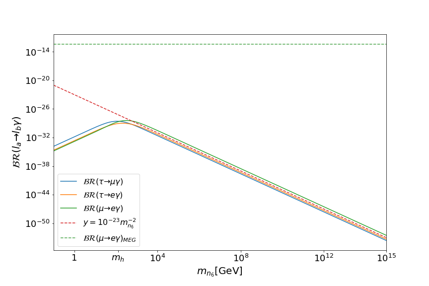
Figure 4: The plot shows $\mathcal{BR}(l_{a}\to l_{b}\gamma)$ (solid lines) in the case of degenerate heavy neutrinos ($m_{n_{4}}=m_{n_{5}}=m_{n_{6}}$). The green dashed lines corresponds to upper bound of $\mu\to e\gamma$ whereas the red dashed line show the curve $y=10^{-23}m_{n_{6}}^{-2}$.

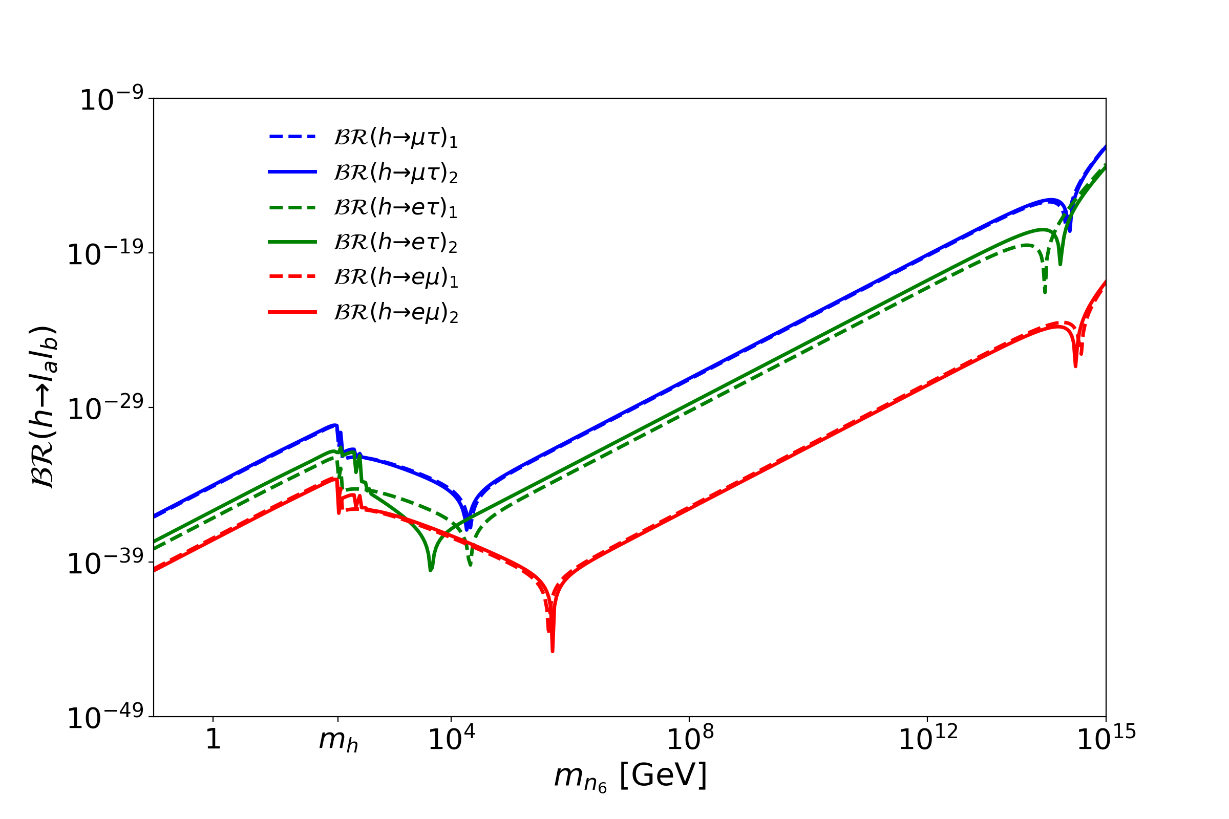
Figure 5: Numerical results for ${\mathcal{BR}}(h\rightarrow l_{a}l_{b})$ in the $\nu SM$ for the two cases: $(i)$ degenerated heavy spectrum (solid lines) with $m_{n_{4}}=m_{n_{5}}=m_{n_{6}}$; $(ii)$ non-degenerated heavy spectrum (dashed lines) with $m_{n_{4}}=m_{n_{6}}/3$ and $m_{n_{5}}=m_{n_{6}}/2$.

For the numerical implementation of the LFV Higgs decays, we consider $\mathbf{U}_{N}=\mathbf{\xi}=\mathbf{I}$, with $\mathbf{I}$ being the identity matrix, as a consequence $\mathbf{M}_{N}=\hat{\mathbf{M}}_{N}$, and we diagonalize numerically the mass matrix (13). The mass matrix depends on the neutrino masses and the mixing matrix $\mathbf{U}_{\mathrm{PMNS}}$. However, it follows from equation (31) valid for the three light neutrino masses, that only the lightest one is independent. Thus, we assume $m_{n_{1}}=10^{-12}$ GeV, which is allowed by the Planck upper bound (32). The heavy neutrino masses will be the free parameters in this work. We consider two cases, $(i)$ degenerate case with $m_{n_{4}}=m_{n_{5}}=m_{n_{6}}$, and $(ii)$ non-degenerate case with $m_{n_{4}}=m_{n_{6}}/3$ and $m_{n_{5}}=m_{n_{6}}/2$. For both cases, we consider $m_{n_{6}}$ in the range $(10^{-1}\text{ GeV},10^{15}\text{ GeV})$. This range respects the two conditions: above this scale it meets the perturvativity constraint Arganda et al. (2015), and below it meets the See-Saw condition $|\mathbf{M}_{D}|<<|\mathbf{M}_{N}|$. Here we remark one difference in this work compared with Thao et al. (2017), namely we use mpmath functions to diagonalize numerically the mass matrix $\mathbf{M}^{\nu}$ (13), which allows to maintain a numerical stable behavior.

In addition, for the degenerate case, from; (34), we can deduce that

$$\mathbf{M}_{D} =i\sqrt{m_{n_{6}}}\mathbf{U}^{*}_{\mathrm{PMNS}}\left(\hat{\mathbf{m}}_{\nu}\right)^{1/2}\quad\Rightarrow\quad\frac{v}{\sqrt{m_{n_{6}}}}\mathbf{Y_{\nu}}=i\mathbf{U}^{*}_{\mathrm{PMNS}}\left(\hat{\mathbf{m}}_{\nu}\right)^{1/2}$$ (35)

$$\frac{v^{2}}{m_{n_{6}}}(\mathbf{Y_{\nu}Y_{\nu}^{\dagger}})_{ab} =(\mathbf{U}^{*}_{\mathrm{PMNS}}\hat{\mathbf{m}}_{\nu}\mathbf{U}^{\top}_{\mathrm{PMNS}})_{ab}\quad\Rightarrow\quad(\mathbf{Y_{\nu}Y_{\nu}^{\dagger}})_{ab}\propto m_{n_{6}}.$$ (36)

On the other hand, from equation (76) we have

$$(\mathbf{M}_{D})_{ab} =(\mathbf{U}^{\nu*}\hat{\mathbf{M}}^{\nu}\mathbf{U}^{\nu\dagger})_{a(b+3)}$$

$$=\sum_{k=1}^{6}U^{\nu*}_{ak}m_{n_{k}}U^{\nu*}_{(b+3)k}$$

$$\approx m_{n_{6}}\sum_{k=4}^{6}U^{\nu*}_{ak}U^{\nu*}_{(b+3)k}\qquad\textrm{with}\,m_{n_{1,2,3}}<<m_{n_{6}}.$$ (37)

On the other hand, from (35) and (37), we can deduce

$$\sum_{k=4}^{6}U^{\nu*}_{ak}U^{\nu*}_{(b+3)k}\approx\frac{i}{\sqrt{m_{n_{6}}}}(\mathbf{U}^{*}_{\mathrm{PMNS}}\left(\hat{\mathbf{m}}_{\nu}\right)^{1/2})_{ab}.$$ (38)

Figure 4 shows the behavior of $\mathcal{BR}(l_{a}\to l_{b}\gamma)$ in the degenerate scenario ($m_{n_{4}}=m_{n_{5}}=m_{n_{6}}$). On the one hand, for $m_{n_{6}}>10^{3}$ GeV, the curve $y=10^{-23}m_{n_{6}}^{-2}$ is a good approximation to $\mathcal{BR}(l_{a}\to l_{b}\gamma)$. On the other hand, an approximation to $\mathcal{BR}(l_{a}\to l_{b}\gamma)$ was previously found by Arganda et al. (2015), which is valid in the regime of heavy neutrino masses, viz, $\mathcal{BR}(l_{a}\to l_{b}\gamma)_{\text{approx}}\propto|\frac{v^{2}}{2m_{n_{6}}^{2}}(\mathbf{Y_{\nu}Y_{\nu}^{\dagger}})_{ab}|^{2}$. So, from equation (36) we conclude that $\mathcal{BR}(l_{a}\to l_{b}\gamma)_{\text{approx}}\propto m_{n_{6}}^{-2}$, and that the experimental upper bound from MEG (see Table 6) to $\mu\to e\gamma$ does not constraint the heavy neutrino mass $m_{n_{6}}$, as illustrated in Figure 4.

Figure 5 shows $\mathcal{BR}(h\to l_{a}l_{b})$ as function of $m_{n_{6}}$, as we expected, ${\mathcal{BR}}(h\to\mu\tau)$ is the largest branching ratio in agreement with literature Pilaftsis (1992); Körner et al. (1993); Arganda et al. (2005); Thao et al. (2017). The highest value is ${\mathcal{BR}}(h\to\mu\tau)\approx 10^{-12}$ with $m_{n_{6}}\simeq 10^{15}\,\textrm{GeV}$ for degenerate and non-degenerate cases. Now, considering ${\mathcal{BR}}(l_{a}\to l_{b}\gamma)$ in the type I See-Saw in Figure 4, the behavior in the region of $m_{n_{6}}\in[10^{-1},10^{4}]$ is similar to ${\mathcal{BR}}(h\to l_{a}l_{b})$. However, in this region, for the LFV Higgs decays the interaction $hn_{i}n_{j}$ is not dominant and diagrams with only one neutrino into the loop are important. Further, when $m_{n_{6}}>10^{4}$ GeV the interaction $hn_{i}n_{j}$ does contribute to loop amplitude for $h\to l_{a}l_{b}$, but it does not contribute to $l_{a}\to l_{b}\gamma$, as a consequence we obtain large ${\mathcal{BR}}(h\to l_{a}l_{b})$.

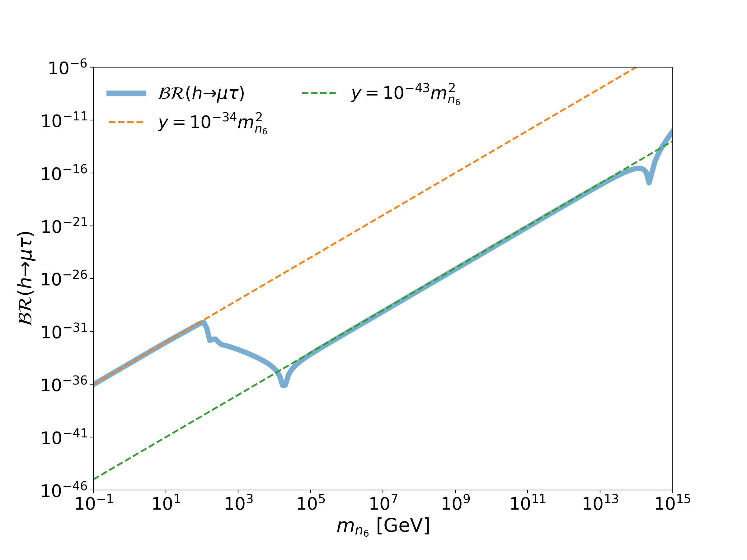
Figure 6: Plot shows the behavior of ${\mathcal{BR}}(h\to\mu\tau)$ vs $m_{n_{6}}$ for the non-degenerate case, and the dashed lines $y\propto m_{n_{6}}^{2}$ fit the ${\mathcal{BR}}(h\to\mu\tau)$ in different regions.

On one hand, in Figure 6, we show the total branching ratio, and the line $y=10^{-34}m_{n_{6}}^{2}$, which coincides with ${\mathcal{BR}}(h\to\mu\tau)$ in the region $m_{n_{6}}\in[10^{-1}\text{ GeV},m_{h}]$, while the line $y=10^{-43}m_{n_{6}}^{2}$ fits the ${\mathcal{BR}}(h\to\mu\tau)$ in $m_{n_{6}}\in(10^{4},10^{15}]$. On the other hand, in Pilaftsis (1992); Körner et al. (1993), an approximate result to ${\mathcal{BR}}(h\to l_{a}l_{b})\propto m_{n}^{4}|F_{N}|^{2}$ with $m_{n}$ denotes the heavy neutrino mass and $F_{N}=U_{bj}^{\nu}C_{ij}U_{ai}^{\nu*}$ is obtained. In our case, from equation (38), this approximate result is equivalent to ${\mathcal{BR}}(h\to l_{a}l_{b})\propto m_{n_{6}}^{2}$ with $F_{N}\propto m_{n}^{-1}$, which is also in agreement with the reported in Thao et al. (2017). However, we found a slight difference in the ${\mathcal{BR}}(h\to\mu\tau)$ and ${\mathcal{BR}}(h\to e\tau)$ in contrast to Thao et al. Thao et al. (2017), specifically showing a gap between these branching ratios, which is a result of the high precision used in the numerical analysis.

As a result of the proportionality of Yukawa couplings to $\sqrt{m_{n_{6}}}$, induced by the Casas-Ibarra parametrization (see equation (35)), an apparent non-decoupling behavior of ${\mathcal{BR}}(h\to\mu\tau)$ is presented, which is also analyzed in Arganda et al. (2015) in the context of the Inverse See-Saw (ISS) model. Although in this case, the Casas-Ibarra parametrization induces that the Yukawa couplings increase as $M_{R}/\sqrt{\mu_{X}}$, where $M_{R}$ is the mass of right-handed heavy neutrinos and $\mu_{X}$ is the mass of the three additional singlets in the ISS, both in the degenerate case. As a result, the maximum values of ${\mathcal{BR}}(h\to\mu\tau)_{ISS}$ are bigger than our results, but the perturvativity limits on Yukawa couplings constraint the heavy neutrino mass $M_{R}$ stronger than in the type I See-Saw model.

In case of Hernández-Tomé et al. (2020), just two new heavy right-handed neutrinos are included with a particular mixing to left-handed neutrinos, as a consequence one simple form of neutrino mass matrix is induced, and the LFV Higgs decays are proportional to the light-heavy mixing angle $s_{\nu_{i}}$. In this work they consider Yukawa couplings proportional to $y_{i}\propto\sqrt{M_{n_{1}}M_{n_{2}}}s_{\nu_{i}}$, which is greater than our assumption with the Casas-Ibarra parametrization. Hence, the perturvativity of Yukawa couplings forbids a large heavy mass scale.

Finally, a descendant behavior of ${\mathcal{BR}}(h\to l_{a}l_{b})$ is shown in Arganda et al. (2005), which agrees with the behavior of ${\mathcal{BR}}(h\to\mu\tau,e\tau)$ and ${\mathcal{BR}}(h\to e\mu)$, in the mass regions $m_{h}<m_{n_{6}}\lesssim 10^{4}$ and $m_{h}<m_{n_{6}}\lesssim 10^{6}$ respectively, as is shown in the Figures 5 and 6.

As a conclusion, the largest values of ${\mathcal{BR}}(h\to\mu\tau)$ are found to be of the order of $\mathcal{O}(10^{-12})$ for $m_{n_{6}}\approx 10^{15}$ GeV. These results are well below the current experimental bounds from LHC et. al. (2020), and it probably works as the lowest possible value for ${\mathcal{BR}}(h\to\tau\mu)$. Furthermore, we notice that ${\mathcal{BR}}(h\to\tau e)$ and ${\mathcal{BR}}(h\to\mu e)$ have lower values than ${\mathcal{BR}}(h\to\tau\mu)$ for most regions of the parameter space.

IV LFV Higgs Decays within the Scotogenic Model

As a second application of our formalism, we shall study the LFV Higgs decays within the Scotogenic Model Ma (2006). The LFV Higgs decays in this model were studied previously. In  Herrero-García et al. (2016) an approximate upper bound was founded, and  Hundi (2022) studied this signals in a region of the parameter space where maximum values to LFV Higgs decays are reached around of ${\mathcal{BR}}(h\to\mu\tau)_{\text{max}}\approx 10^{-7}$. We present the features of this model in the following.

IV.1 Model content and parameters

The matter content of the Scotogenic Model with the group $SU(2)_{L}\otimes U(1)_{Y}\otimes Z_{2}$ is given by Ma (2006):

$$\begin{array}[]{c}\left(\nu_{La},l_{La}\right)\sim(2,-1/2,+),\quad l_{Ra}\sim(1,1,+),\quad N_{Rk}\sim(1,0,-),\cr\left(\phi^{+},\phi^{0}\right)\sim(2,1/2,+),\quad\left(\eta^{+},\eta^{0}\right)\sim(2,1/2,-),\end{array}$$

where an inert doublet $\eta$ and three right-handed neutrinos $N_{Ri}$ odd under $Z_{2}$ symmetry have been included. Yukawa sector allows the interaction between left and right-handed neutrinos with scalar doublet $\eta$:

$$\mathcal{L}_{Y}=f_{ab}\left(\phi^{-}\nu_{La}+\overline{\phi_{0}}l_{La}\right)l_{Rb}+Y^{\prime}_{ab}\left(\nu_{La}\eta_{0}-l_{La}\eta^{+}\right)N_{Rb}+\textrm{H. c.}$$ (39)

and the Majorana term for right-handed neutrinos is added,

$$\frac{1}{2}M_{k}\overline{N_{Rk}}^{c}N_{Rk}+\textrm{H. c.},$$ (40)

being $M_{k}$ the mass of $N_{Rk}$. In this case, the more general scalar potential under $Z_{2}$ symmetry is as follows,

$$V(\Phi,\eta) =\mu_{1}^{2}\left(\Phi^{\dagger}\Phi\right)+\mu_{2}^{2}\left(\eta^{\dagger}\eta\right)+\frac{\lambda_{1}}{2}\left(\Phi^{\dagger}\Phi\right)^{2}+\frac{\lambda_{2}}{2}\left(\eta^{\dagger}\eta\right)^{2}$$ (41)

$$+\lambda_{3}\left(\Phi^{\dagger}\Phi\right)\left(\eta^{\dagger}\eta\right)+\lambda_{4}\left(\Phi^{\dagger}\eta\right)\left(\eta^{\dagger}\Phi\right)+\frac{\lambda_{5}}{2}\left[\left(\Phi^{\dagger}\eta\right)^{2}+\textrm{H. c.}\right].$$

The mass spectrum to new scalar particles is

$$m^{2}\left(\sqrt{2}Re\phi_{0}\right) = m_{h}^{2} =2\lambda_{1}v^{2},$$ (42)

$$m^{2}\left(\eta^{\pm}\right) = m_{\eta}^{2} =\frac{\lambda_{3}v^{2}}{2}+\mu_{2}^{2},$$

$$m^{2}\left(\sqrt{2}\mathit{Re}\eta_{0}\right) = m_{R}^{2} =2\mu_{2}^{2}+v^{2}\left(\lambda_{3}+\lambda_{4}+\lambda_{5}\right),$$

$$m^{2}\left(\sqrt{2}\mathit{Im}\eta_{0}\right) = m_{I}^{2} =2\mu_{2}^{2}+v^{2}\left(\lambda_{3}+\lambda_{4}-\lambda_{5}\right),$$

and SM-like Higgs is associated to $h=\sqrt{2}\mathit{Re}\phi_{0}$.

Neutrino mass is generated by a radiative See-Saw mechanism and is given by

$$\left(\mathbf{\mathcal{M}}_{\nu}\right)_{ij}=Y^{\prime}_{ik}Y^{\prime}_{jk}M_{k}\frac{1}{16\pi^{2}}\left[\left(\frac{m_{R}^{2}}{M_{k}^{2}-m_{R}^{2}}\log\frac{m_{R}^{2}}{M_{k}^{2}}\right)-\left(\frac{m_{I}^{2}}{M_{k}^{2}-m_{I}^{2}}\log\frac{m_{I}^{2}}{M_{k}^{2}}\right)\right],$$ (43)

where $m_{R}$, $m_{I}$, $m_{\eta}$ and $M_{k}$ are the masses of $\eta_{R}$, $\eta_{I}$, $\eta^{\pm}$ and $N_{Ri}$ respectively. Also, $k$ index runs over heavy neutrino masses. This matrix can be rewritten in a matrix notation as $\mathbf{\mathcal{M}}_{\nu}=\mathbf{Y^{\prime}}\mathbf{D}_{\Lambda}\mathbf{Y^{\prime}}^{\top}$, where

$$\begin{array}[]{rcl}\mathbf{D}_{\Lambda}&=&\text{diag}(\Lambda_{1},\Lambda_{2},\Lambda_{3}),\\ \Lambda_{k}&=&\frac{M_{k}}{16\pi^{2}}\left[\left(\frac{m_{R}^{2}}{M_{k}^{2}-m_{R}^{2}}\log\frac{m_{R}^{2}}{M_{k}^{2}}\right)-\left(\frac{m_{I}^{2}}{M_{k}^{2}-m_{I}^{2}}\log\frac{m_{I}^{2}}{M_{k}^{2}}\right)\right].\end{array}$$ (44)

Then, if we choose the basis where Yukawa matrix $\mathbf{Y}^{\prime}$ is diagonal, $\mathbf{\mathcal{M}}_{\nu}$ is diagonal too. So, we can rewrite the Yukawa matrix as follows,

$$\mathbf{Y^{\prime}}=\text{diag}\left(\sqrt{\frac{m_{\nu_{1}}}{\Lambda_{1}}},\sqrt{\frac{m_{\nu_{2}}}{\Lambda_{2}}},\sqrt{\frac{m_{\nu_{3}}}{\Lambda_{3}}}\right)\quad\text{or}\quad Y^{\prime}_{ij}=\sqrt{\frac{m_{\nu_{i}}}{\Lambda_{i}}}\delta_{ij},$$ (45)

where $m_{\nu_{i}}$ ($i,j=1,2,3$) are the light neutrino masses in normal order. However, as we have noticed, in this basis the matrix to diagonalize the neutrino mass matrix, $\mathbf{V}_{L}^{\nu}$ is equal to identity. On the other hand, the mass matrix of charged leptons will be rotated by $\mathbf{V}_{L}^{l}$ to go to the physical basis. Thus, the neutrino mixing matrix is $\mathbf{U}_{\mathrm{PMNS}}=\mathbf{V}_{L}^{\nu\dagger}\mathbf{V}_{L}^{l}=\mathbf{V}_{L}^{l}$. Finally, in the physical basis, new Yukawa couplings for the interaction between left-handed lepton doublet and singlet neutrinos given by

$$\mathbf{Y}=\mathbf{Y^{\prime}}\mathbf{U}_{\mathrm{PMNS}}.$$ (46)

However, by means of equation (45) and (46) we have that

$$(\mathbf{Y}^{\dagger}\mathbf{Y})_{ij}=Y_{ki}^{*}Y_{kj}=\frac{m_{\nu_{k}}}{\Lambda_{k}}U_{ki}^{*}U_{kj},$$ (47)

which will allow the use of the GIM mechanism in the loop calculation.

Vertex	Coupling	Vertex	Coupling
$hG^{+}G^{-}$	$-i\frac{m_{h}^{2}}{v}$	$h\eta^{+}\eta^{-}$	$-\frac{2i\left(m_{\eta}^{2}-\mu_{2}^{2}\right)}{v}$
$G^{-}l^{+}_{a}\nu_{k}$	$i\frac{\sqrt{2}}{v}m_{a}U^{*}_{ka}P_{L}$	$G^{+}l^{-}_{b}\nu_{k}$	$i\frac{\sqrt{2}}{v}m_{b}U_{kb}P_{R}$
$hG^{+}W^{-}$	$-\frac{i}{2}g(p_{+}-p_{0})_{\mu}$	$hW^{+}G^{-}$	$-\frac{i}{2}g(p_{0}-p_{-})_{\mu}$
$W^{-}l^{+}_{a}\nu_{k}$	$-i\frac{g}{\sqrt{2}}U^{*}_{ka}\gamma_{\mu}P_{L}$	$W^{+}l^{-}_{b}\nu_{k}$	$-i\frac{g}{\sqrt{2}}U_{kb}\gamma_{\mu}P_{L}$
$\eta^{-}l^{+}_{a}N_{k}$	$iY^{*}_{ka}P_{R}$	$\eta^{+}l^{-}_{a}N_{k}$	$iY_{kb}P_{L}$
$hW^{+}_{\mu}W^{-}_{\nu}$	$igm_{W}g_{\mu\nu}$

Table 5: Couplings involved in the LFV Higgs decays for the Scotogenic model. The $p_{0}$, $p_{+}$ and $p_{-}$ are incoming momenta of $h$, $G^{+}$ and $G^{-}$, respectively.

IV.2 Model constraints

Although the Scotogenic model is a minimal extension of SM, it describes a wide spectrum of phenomena such as: massive neutrinos, fermionic dark matter or LFV processes, each of these phenomena gives some constraints on the parameter space. Next, we describe the constraints that are used to derive the allowed regions of parameter space.

• Electroweak parameters $(S,T,U)$. For the case where $U=0$, the experimental values of the parameters $S$ and $T$ are: $S=0.0\pm 0.07,\,T=0.05\pm 0.06$ Zyla et al. (2020). The analytic expressions for these parameters can be obtained from Ref. Grimus et al. (2008). As a consequence of these constraints, the masses of scalar inert particles are very close to each other.

• Charged Lepton Flavor Violation. The LFV processes $l_{b}\to l_{a}\gamma$ are a consequence of neutrino masses, and experimentally they have been highly restricted, as it is summarized in Table 6.

  Process	Experimental bound
  $\mathcal{BR}(\mu\rightarrow e\gamma)$	$4.2\times 10^{-13}$Baldini et al. (2016)
  $\mathcal{BR}(\tau\rightarrow e\gamma)$	$3.3\times 10^{-8}$Aubert et al. (2010)
  $\mathcal{BR}(\tau\rightarrow\mu\gamma)$	$4.2\times 10^{-8}$Uno et al. (2021)

  Table 6: Experimental upper bounds for CLFV processes.

  In the Scotogenic model, the branching ratio of these processes are given by Toma and Vicente (2014):

  $$\mathcal{BR}(l_{b}\rightarrow l_{a}\gamma)=\frac{3(4\pi)^{3}\alpha}{4G_{F}^{2}}|A_{D}|^{2}\mathcal{BR}(l_{b}\rightarrow l_{a}\nu_{b}\bar{\nu_{a}}),$$ (48)

  where $A_{D}=\sum_{i=1}^{3}\frac{Y_{ki}^{*}Y_{kj}}{2(4\pi)^{2}}\frac{1}{m_{\eta}^{2}}F\left(\frac{M_{k}^{2}}{m_{\eta}^{2}}\right)$, and $F(x)=\frac{1-6x+3x^{2}+2x^{3}-6x^{2}\log{x}}{6(1-x)^{4}}$. The experimental limits are $\mathcal{BR}\left(\tau\rightarrow\mu\nu\bar{\nu}\right)=0.1739\pm 0.0004$, $\mathcal{BR}\left(\tau\rightarrow e\nu\bar{\nu}\right)=0.1782\pm 0.0004$, and $\mathcal{BR}\left(\mu\rightarrow e\nu\bar{\nu}\right)\approx 1$ Zyla et al. (2020).

• Fermionic dark matter The experimental value of the relic density of dark matter $\Omega\hat{h}^{2}$ is $\Omega\hat{h}^{2}=0.12\pm 0.0012$. In the Scotogenic model the $Z_{2}$ symmetry allows for both boson and fermion dark matter candidates, we choose the case of the lightest singlet neutrino $N_{1}$ as cold fermionic dark matter. The parameter $\Omega\hat{h}^{2}$ is related to annihilation cross section $\sigma_{ann}$ by Ho and Tandean (2013b); Kubo et al. (2006b); Jungman et al. (1996):

  $$\Omega\hat{h}^{2}=\frac{1.07\times 10^{9}x_{f}\text{GeV}^{-1}}{\sqrt{g_{*}}m_{Pl}(\hat{a}+3(\hat{b}-\hat{a}/4))/x_{f}},$$ (49)

  where $x_{f}=\ln[0.955(\hat{a}+6\hat{b}/x_{f})M_{1}m_{Pl}]/\sqrt{g_{*}x_{f}}$, and $\hat{h}$ denotes the Hubble parameter, $m_{Pl}=1.22\times 10^{19}$ GeV is the Planck mass, $g_{*}$ is the number of relativistic degrees of freedom below the freeze-out temperature $T_{f}=M_{N_{1}}/x_{f}$; $\hat{a}$ and $\hat{b}$ are defined by the expansion $\sigma_{ann}v_{\text{rel}}=\hat{a}+\hat{b}v_{\text{rel}^{2}}+O(v_{\text{rel}}^{4})$, in terms of the relative speed $v_{\text{rel}}$ of the $N_{1}\overline{N}_{1}$ pair in their center-of-mass frame. At tree level, the processes $N_{1}\overline{N}_{1}\rightarrow l_{i}^{+}l_{j}^{-}$ and $N_{1}\overline{N}_{1}\rightarrow\nu_{i}\overline{\nu}_{j}$ mediated by $\eta^{\pm}$ and $\eta_{R,I}$ respectively, are the only ones which contribute to $\sigma_{ann}$. In the limit when all final masses neglected, their combined cross section times $v_{\text{rel}}$ is expressed as Ho and Tandean (2013b)

  $$\begin{split}\sigma_{ann}v_{rel}&=\sum_{i,j=1,2,3}\frac{\left|Y_{i1}Y_{j1}\right|^{2}M_{1}^{2}v_{\mathrm{rel}}^{2}}{48\pi}\left[\frac{M_{1}^{4}+m_{\eta}^{4}}{\left(M_{1}^{2}+m_{\eta}^{2}\right)^{4}}+\frac{M_{1}^{4}+m_{0}^{4}}{\left(M_{1}^{2}+m_{0}^{2}\right)^{4}}\right],\end{split}$$ (50)

  with $m_{0}^{2}=(m_{R}^{2}+m_{I}^{2})/2$. Although (50) shows the main dependence of $\sigma_{ann}v_{rel}$, the relic density of dark matter provides a strong constraint, together with LFV process. To improve the numerical precision, we include the charged lepton masses in the numerical analysis.

IV.2.1 Allowed parameter space

The parameter space consists of heavy neutrino masses $M_{k}$, where $M_{1}$ is the mass of the dark matter candidate, also, it depends on inert scalar masses $m_{\eta}$, $m_{R}$, light neutrino mass $m_{1}$ and finally parameters $\lambda_{2,5}$ and $\mu_{2}^{2}$ from scalar potential. We have found an allowed parameter space fixing $\lambda_{2}=0.1$ (which only affects the scalar sector) and $m_{1}=m_{1}^{\text{max}}=3.01\times 10^{-11}$ GeV which fulfill the Planck satellite upper bound on light neutrino masses. Then a random scan is performed considering the follows ranges for the parameter space

$$1\,\text{GeV}<M_{1}<1\,\text{TeV};\quad 10\,\text{TeV}<M_{2,3}<50\,\text{TeV};$$

$$100\,\text{GeV}<m_{R,\eta}<1\,\text{TeV};\quad$$

$$10^{-11}<\lambda_{5}<10^{-8};\quad|\lambda_{3,4}|<4\pi;\quad M_{1}<m_{R,I,\eta},M_{2,3}.$$ (51)

From the scalar spectrum we can deduce the relation $\mu_{2}^{2}=m_{R}^{2}-m_{\eta}^{2}-v^{2}(\lambda_{3}/2+\lambda_{4}+\lambda_{5})$, which is assumed in this analysis. The final constraint of (IV.2.1) guarantees that $N_{1}$ is a viable candidate for dark matter. The allowed parameter space is projected on different planes as it is shown in Figures 7 and 8. The parameter space is strongly constrained for $m_{\eta}$, $m_{R}$ and dark matter mass $M_{1}$, mainly by the CLFV $l_{b}\to l_{a}\gamma$ process and dark matter relic density bounds. In addition, $\lambda_{5}$ is tiny because of the degeneracy between $m_{R}$ and $m_{I}$, which guarantees light neutrino masses and the other constraints. Finally, we also conclude from this scan that $\lambda_{5}\approx 10^{-10}$ and the heavy neutrino masses $M_{2,3}$ are not constrained in such region.

Figure 7: Allowed parameter space for $M_{1}$, $m_{\eta}$ and $m_{R}$. The left plot shows that $m_{\eta}\approx M_{1}$, whereas right plot shows $m_{R}\gtrapprox M_{1}$.

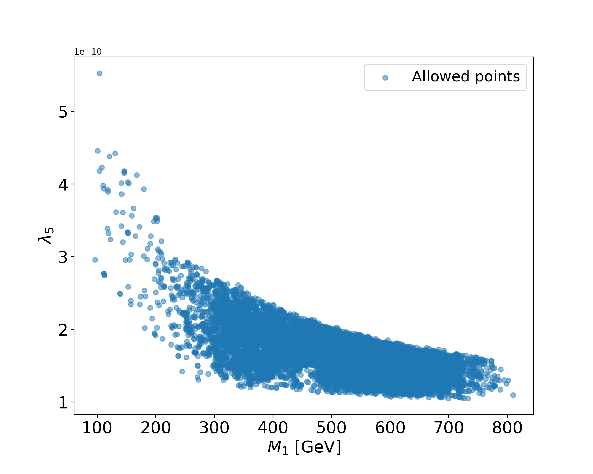
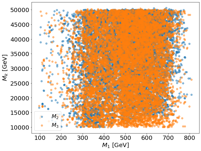
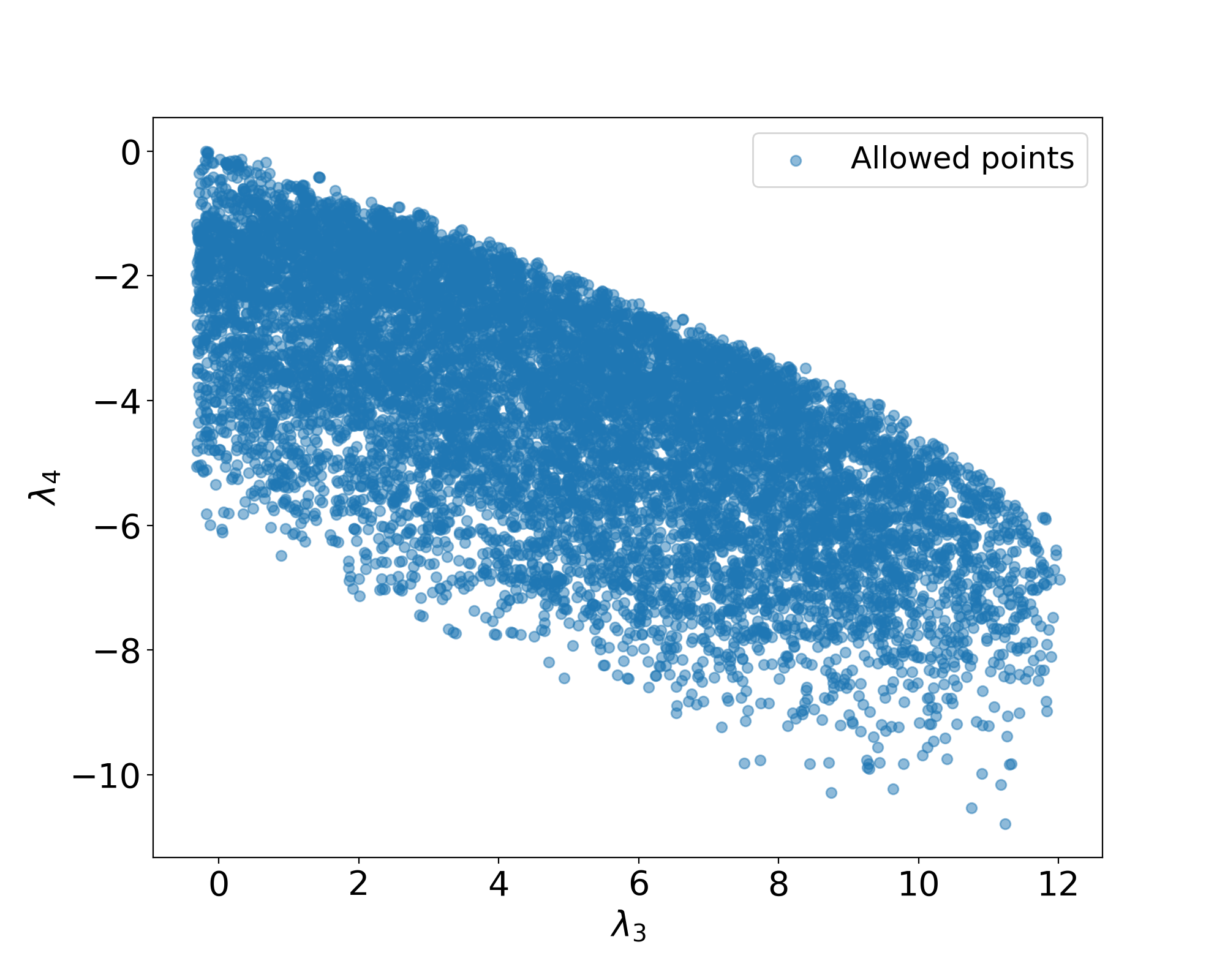
Figure 8: Allowed parameter space for $M_{1,2,3}$ and $\lambda_{3,4,5}$. It is observed from plane $\lambda_{5}$ vs $M_{1}$ that $\lambda_{5}\approx 10^{-10}$. The masses of $M_{2,3}\gg M_{1}$ comes from top right plot. Finally, we have that $-10.8<\lambda_{4}\lessapprox 0.02$ and $0\lessapprox\lambda_{3}\lessapprox 12$ in the bottom plot.

IV.3 Form factors for the amplitude of the decay $h\to l_{a}^{+}l_{b}^{-}$

It is observed as a consequence of $Z_{2}$ symmetry that diagrams for LFVHD in the Scotogenic model which contain light and heavy neutrinos are separate, also, in this model, the interaction $hn_{i}n_{j}$, with $n_{i}$ a light or heavy neutrino it is not allowed, as a consequence we only have diagrams with one neutrino inside the loop. The relevant couplings have been calculated with SARAH package Staub (2014) and are given in Table 5 and the associated diagrams are calculated in the next two subsections.

IV.3.1 Heavy neutrino contributions

In this model, heavy neutrinos only interact with other heavy neutrinos or inert scalar fields. The last ones can interact with SM Higgs boson by means of scalar potential couplings (41). All of these interactions are given in Table 5. Allowed diagrams are summarized in the first three rows of Table 7 and shown in Figure 9.

(a) FSS-like.

(b) FS-like.

(c) SF-like.

Figure 9: Heavy neutrino diagrams of LFV Higgs decays in the Scotogenic model. The sub-captions show the respective generic structure of each diagram.

	Diagram(Figure)	$P_{0}$	$P_{1}$	$P_{2}$
1	FSS(9(a))	$N_{k}$	$\eta$	$\eta$
2	FS(9(b))	$N_{k}$	$\eta$	—
3	SF(9(c))	$N_{k}$	—	$\eta$
4	FSS(10(a))	$\nu_{k}$	$G^{\pm}$	$G^{\mp}$
5	FSV(10(b))	$\nu_{k}$	$G^{\pm}$	$W^{\mp}$
6	FVS(10(c))	$\nu_{k}$	$W^{\pm}$	$G^{\mp}$
7	FVV(10(d))	$\nu_{k}$	$W^{\pm}$	$W^{\mp}$
8	FS(10(e))	$\nu_{k}$	$G^{\pm}$	—
9	FV(10(f))	$\nu_{k}$	$W^{\pm}$	—
10	SF(10(g))	$\nu_{k}$	—	$G^{\pm}$
11	VF(10(h))	$\nu_{k}$	—	$W^{\pm}$

Table 7: Particles involved in each one-loop diagram that contribute to $h\to l_{a}^{+}l_{b}^{-}$ in the Scotogenic model. Second column shows the structure (figure) of each diagram associated to the Figures 9 and 10. The remaining columns identify the particles $P_{k}$ inside the loop.

As a consequence, the dependence of PV functions is given by

$$\operatorname{C_{0,1,2}} =\operatorname{C_{0,1,2}}{\left(m_{{N_{k}}},m_{{\eta}},m_{{\eta}}\right)},$$

$$\operatorname{B_{1}^{(s)}} =\operatorname{B_{1}^{(s)}}{\left(m_{{N_{k}}},m_{{\eta}}\right)},$$

$$\operatorname{B_{0}^{(12)}} =\operatorname{B_{0}^{(12)}}{\left(m_{{\eta}},m_{{\eta}}\right)},$$

with $s=1,2$. Then, the form factors to heavy neutrinos contributions can be calculated with our results as follows.

Diagram 9(a): FSS structure

This diagram has an FSS structure and two types of couplings are present, which can be decomposed in terms of the coupling constants. Following the structure of our generic vertexes, as given in equations (II), (II), Figure 1 and the Table 5, as follows:

$$c_{h}^{S^{\pm}(1)}(h\eta^{-}\eta^{+}) =-\frac{2i\left(m_{\eta}^{2}-\mu_{2}^{2}\right)}{v};$$ (53)

$$c_{R}^{S^{+}(2)}(\eta^{+}l_{b}^{-}N_{k}) =0; c_{L}^{S^{+}(2)}(\eta^{+}l_{b}^{-}N_{k}) =iY_{bk};$$

$$c_{R}^{S^{-}(3)}(\eta^{-}l_{a}^{+}N_{k}) =iY_{ak}^{*}; c_{L}^{S^{-}(3)}(\eta^{-}l_{a}^{+}N_{k}) =0.$$

Then, by means of equation (11) the form factors are given by:

$$A_{R}^{h}(N_{k}\eta^{+}\eta^{-})_{ab} =c^{S^{\pm}(1)}_{h}(h\eta^{+}\eta^{-})c_{L}^{S^{+}(2)}(\eta^{+}l_{b}^{-}N_{k})c_{R}^{S^{-}(3)}(\eta^{-}l_{a}^{+}N_{k})\mathcal{H}_{RL}(N_{k}\eta^{+}\eta^{-})$$

$$=-\frac{2i\left(m_{\eta}^{2}-\mu_{2}^{2}\right)}{v}iY_{kb}\,iY_{ka}^{*}\left(\frac{i}{16\pi^{2}}(-m_{b}\operatorname{C}_{1})\right)$$

$$=\frac{m_{b}}{8\pi^{2}v}\left(m_{\eta}^{2}-\mu_{2}^{2}\right)\operatorname{C}_{1}Y_{bk}\,Y_{ak}^{*},$$ (54a)

$$A_{L}^{h}(N_{k}\eta^{+}\eta^{-})_{ab} =c^{S^{\pm}(1)}_{h}(h\eta^{+}\eta^{-})c_{L}^{S^{+}(2)}(\eta^{+}l_{b}^{-}N_{k})c_{R}^{S^{-}(3)}(\eta^{-}l_{a}^{+}N_{k})\mathcal{H}_{LR}(N_{k}\eta^{+}\eta^{-})$$

$$=-\frac{2i\left(m_{\eta}^{2}-\mu_{2}^{2}\right)}{v}iY_{bk}\,iY_{ak}^{*}\left(\frac{i}{16\pi^{2}}(m_{a}\operatorname{C}_{1})\right)$$

$$=-\frac{m_{a}}{8\pi^{2}v}\left(m_{\eta}^{2}-\mu_{2}^{2}\right)\operatorname{C}_{1}Y_{bk}\,Y_{ak}^{*}.$$ (54b)

We have included the factor $i/16\pi^{2}$ which comes from dimensional regularization, for more details see Appendix B.

Diagrams 9(b) and 9(c): FS and SF structures

For these two diagrams, we only replace $c_{h}^{S^{\pm}(1)}(h\eta^{+}\eta^{-})$ by

$$c_{h}^{F^{\pm}(1)}(hl_{a}^{-}l_{a}^{+})=\frac{igm_{a}}{2m_{W}}$$

, where $m_{a}$ is the mass of the charged lepton $l_{a}$. Therefore, by equation (11) the form factors for diagrams 9(b) and  9(c) are

$$A_{R}^{h}(N_{l}\eta)_{ab} =m_{ab}^{-2}c^{F^{\pm}(1)}_{h}(hl_{b}^{-}l_{b}^{+})c_{L}^{S^{+}(2)}(\eta^{+}l_{b}^{-}N_{k})c_{R}^{S^{-}(3)}(\eta^{-}l_{a}^{+}N_{k})\mathcal{H}_{LR}(N_{k}\eta)$$

$$=\frac{igm_{b}}{2m_{W}m_{ab}^{2}}iY_{kb}\,iY_{ka}^{*}\left(\frac{i}{16\pi^{2}}(m_{a}^{2}\operatorname{B}_{1}^{(1)})\right)$$

$$=\frac{gm_{a}^{2}m_{b}}{32\pi^{2}m_{W}m_{ab}^{2}}\operatorname{B}_{1}^{(1)}Y_{bk}\,Y_{ak}^{*},$$ (55a)

$$A_{L}^{h}(N_{k}\eta)_{ab} =m_{ab}^{-2}c^{F^{\pm}(1)}_{h}(hl_{b}^{-}l_{b}^{+})c_{L}^{S^{+}(2)}(\eta^{+}l_{b}^{-}N_{k})c_{R}^{S^{-}(3)}(\eta^{-}l_{a}^{+}N_{k})\mathcal{H}_{RL}(N_{k}\eta)$$

$$=\frac{igm_{b}}{2m_{W}m_{ab}^{2}}iY_{kb}\,iY_{ka}^{*}\left(\frac{i}{16\pi^{2}}(m_{a}m_{b}\operatorname{B}_{1}^{(1)})\right)$$

$$=\frac{gm_{a}m_{b}^{2}}{32\pi^{2}m_{W}m_{ab}^{2}}\operatorname{B}_{1}^{(1)}Y_{bk}\,Y_{ak}^{*},$$ (55b)

$$A_{R}^{h}(\eta N_{k})_{ab} =m_{ab}^{-2}c^{F^{\pm}(1)}_{h}(hl_{a}^{-}l_{a}^{+})c_{L}^{S^{+}(2)}(\eta^{+}l_{b}^{-}N_{k})c_{R}^{S^{-}(3)}(\eta^{-}l_{a}^{+}N_{k})\mathcal{H}_{LR}(\eta N_{k})$$

$$=\frac{igm_{a}}{2m_{W}m_{ab}^{2}}iY_{kb}\,iY_{ka}^{*}\left(\frac{i}{16\pi^{2}}(m_{a}m_{b}\operatorname{B}_{1}^{(2)})\right)$$

$$=\frac{gm_{a}^{2}m_{b}}{32\pi^{2}m_{W}m_{ab}^{2}}\operatorname{B}_{1}^{(2)}Y_{bk}\,Y_{ak}^{*},$$ (55c)

$$A_{L}^{h}(\eta N_{k})_{ab} =m_{ab}^{-2}c^{F^{\pm}(1)}_{h}(hl_{a}^{-}l_{a}^{+})c_{L}^{S^{+}(2)}(\eta^{+}l_{b}^{-}N_{k})c_{R}^{S^{-}(3)}(\eta^{-}l_{a}^{+}N_{k})\mathcal{H}_{RL}(\eta N_{k})$$

$$=\frac{igm_{a}}{2m_{W}m_{ab}^{2}}iY_{kb}\,iY_{ka}^{*}\left(\frac{i}{16\pi^{2}}(m_{b}^{2}\operatorname{B}_{1}^{(2)})\right)$$

$$=\frac{gm_{a}m_{b}^{2}}{32\pi^{2}m_{W}m_{ab}^{2}}\operatorname{B}_{1}^{(2)}Y_{bk}\,Y_{ak}^{*}.$$ (55d)

Divergences are canceled after sum the form factors of diagrams 9(b) and 9(c). If we denote the loop particles by $\Xi_{N_{k}}=\{N_{k}\eta\eta,N_{k}\eta,\eta N_{k}\}$, in all the heavy neutrino contributions, the total form factors for heavy neutrinos contribution are as follows:

$$A_{L,R}^{h}(N)_{ab} =\sum_{k=1}^{3}\left(A_{L,R}^{h}(N_{k}\eta^{+}\eta^{-})_{ab}+A_{L,R}^{h}(N_{k}\eta^{+})_{ab}+A_{L,R}^{h}(\eta^{+}N_{k})_{ab}\right)$$

$$=\sum_{k=1}^{3}\sum_{\xi_{k}\in\Xi_{N_{k}}}A_{L,R}^{h}(\xi_{k})_{ab}.$$ (56)

IV.3.2 Light neutrino contributions

Next, we consider the diagrams 4-11 shown in Table 7 and Figure 10, in this case the particles that contribute to the loop are Goldstone bosons $G^{\pm}$, vector bosons $W^{\pm}$ and light neutrinos. In Feynman t’Hoft gauge, the Goldstone boson propagator contains $m_{W^{\pm}}$, then Passarino-Veltman functions will have the following mass dependence:

$$\operatorname{C_{0,1,2}} =\operatorname{C_{0,1,2}}{\left(m_{{\nu_{k}}},m_{{W}},m_{{W}}\right)},$$

$$\operatorname{B_{1}^{(s)}} =\operatorname{B_{1}^{(s)}}{\left(m_{{\nu_{k}}},m_{{W}}\right)},$$

$$\operatorname{B_{0}^{(12)}} =\operatorname{B_{0}^{(12)}}{\left(m_{{W}},m_{{W}}\right)}.$$

(a) FSS-like

(b) FSV-like

(c) FVS-like

(d) FVV-like

(e) FS-like

(f) FV-like

(g) SF-like

(h) VF-like

Figure 10: Light neutrino diagrams contribution to LFV Higgs decays in the Scotogenic model. The sub-captions denote the respective generic structure of each diagram.

Similarly, as we did for heavy neutrino contributions and following the result of equation (11) and Table 1, we obtain the form factors for light neutrino contribution, as given in Table 8.

$\xi_{k}$(Figure)	$A^{h}_{R}(\xi_{k})_{ab}$	$A^{h}_{L}(\xi_{k})_{ab}$
$\nu_{k}G^{-}G^{+}$(10(a))	$-\frac{m_{h}^{2}m_{a}^{2}m_{b}}{8\pi^{2}v^{3}}\operatorname{C_{1}}{U}_{bk}{U}_{ak}^{*}$	$\frac{m_{h}^{2}m_{a}m_{b}^{2}}{8\pi^{2}v^{3}}\operatorname{C_{2}}{U}_{bk}{U}_{ak}^{*}$
$\nu_{k}G^{-}W^{+}$(10(b))	$-\frac{g^{2}m_{a}^{2}m_{b}}{32\pi^{2}v}\left(\operatorname{C_{1}}-2\operatorname{C_{2}}\right){U}_{bk}{U}_{ak}^{*}$	$\frac{g^{2}m_{a}}{32\pi^{2}v}\left(m_{a}^{2}\operatorname{C}_{1}+2(m_{h}^{2}-m_{a}^{2})\operatorname{C}_{2}-X\right){U}_{bk}{U}_{ak}^{*}$
$\nu_{k}W^{-}G^{+}$(10(c))	$-\frac{g^{2}m_{b}}{32\pi^{2}v}\left(X+m_{b}^{2}\operatorname{C}_{2}+2(m_{h}^{2}-m_{b}^{2})\operatorname{C}_{1}\right){U}_{bk}{U}_{ak}^{*}$	$\frac{g^{2}m_{a}m_{b}^{2}}{32\pi^{2}v}\left(\operatorname{C}_{2}-2\operatorname{C}_{1}\right){U}_{bk}{U}_{ak}^{*}$
$\nu_{k}W^{-}W^{+}$(10(d))	$\frac{g^{4}m_{b}v}{32\pi^{2}}\operatorname{C_{2}}{U}_{bk}{U}_{ak}^{*}$	$-\frac{g^{4}m_{a}v}{32\pi^{2}}\operatorname{C_{1}}{U}_{bk}{U}_{ak}^{*}$
$\nu_{k}G^{\pm}$(10(e))	$\frac{\sqrt{2}gm_{a}^{2}m_{b}^{3}}{32\pi^{2}m_{W}v^{2}m_{ab}^{2}}\operatorname{{{B^{(1)}_{1}}}}{U}_{bk}{U}_{ak}^{*}$	$\frac{\sqrt{2}gm_{a}^{3}m_{b}^{2}}{32\pi^{2}m_{W}v^{2}m_{ab}^{2}}\operatorname{{{B^{(1)}_{1}}}}{U}_{bk}{U}_{ak}^{*}$
$\nu_{k}W^{\pm}$(10(f))	$\frac{\sqrt{2}g^{3}m_{a}^{2}m_{b}}{64\pi^{2}m_{W}m_{ab}^{2}}\operatorname{{{B^{(1)}_{1}}}}{U}_{bk}{U}_{ak}^{*}$	$\frac{\sqrt{2}g^{3}m_{a}m_{b}^{2}}{64\pi^{2}m_{W}m_{ab}^{2}}\operatorname{{{B^{(1)}_{1}}}}{U}_{bk}{U}_{ak}^{*}$
$G^{\pm}\nu_{k}$(10(g))	$\frac{\sqrt{2}gm_{a}^{2}m_{b}^{3}}{32\pi^{2}m_{W}v^{2}m_{ab}^{2}}\operatorname{{{B^{(2)}_{1}}}}{U}_{bk}{U}_{ak}^{*}$	$\frac{\sqrt{2}gm_{a}^{3}m_{b}^{2}}{32\pi^{2}m_{W}v^{2}m_{ab}^{2}}\operatorname{{{B^{(2)}_{1}}}}{U}_{bk}{U}_{ak}^{*}$
$W^{\pm}\nu_{k}$ (10(h))	$\frac{\sqrt{2}g^{3}m_{a}^{2}m_{b}}{64\pi^{2}m_{W}m_{ab}^{2}}\operatorname{{{B^{(2)}_{1}}}}{U}_{bk}{U}_{ak}^{*}$	$\frac{\sqrt{2}g^{3}m_{a}m_{b}^{2}}{64\pi^{2}m_{W}m_{ab}^{2}}\operatorname{{{B^{(2)}_{1}}}}{U}_{bk}{U}_{ak}^{*}$

Table 8: Form factors for light neutrino contributions in the Scotogenic model.

Divergences for these form factors are canceled, to see it, we sum over the form factors of diagrams 10(e) with  10(g), and 10(f) with 10(h).

Finally, if we denote $\Xi_{\nu_{k}}=\{\nu_{k}G^{+}G^{-},\nu_{k}G^{+}W^{-},\nu_{k}W^{+}G^{-},\nu_{k}W^{+}W^{-},\nu_{k}G+,G^{+}\nu_{k},\nu_{k}W^{+},W^{+}\nu_{k}\}$ as the set of all light neutrino contributions, the total form factors for light neutrinos contribution are given by:

$$A_{L,R}^{h}(\nu)_{ab} =\sum_{k=1}^{3}\left(A_{L,R}^{h}(\nu_{k}G^{+}G^{-})_{ab}+A_{L,R}^{h}(\nu_{k}G^{+}W^{-})_{ab}+A_{L,R}^{h}(\nu_{k}W^{+}G^{-})_{ab}+A_{L,R}^{h}(\nu_{k}W^{+}W^{-})_{ab}\right.$$

$$\left.+A_{L,R}^{h}(\nu_{k}G^{+})_{ab}+A_{L,R}^{h}(G^{+}\nu_{k})_{ab}+A_{L,R}^{h}(\nu_{k}W^{+})_{ab}+A_{L,R}^{h}(W^{+}\nu_{k})_{ab}\right)$$

$$=\sum_{k=1}^{3}\sum_{\xi_{k}\in\Xi_{\nu_{k}}}A_{L,R}^{h}(\xi_{k})_{ab}.$$ (58)

IV.4 Numerical analysis of $\mathcal{BR}(h\to l_{a}l_{b})$

From the results of previous section, we have that light neutrino contribution depends only on the neutrino masses and the mixing matrix $\mathbf{U}^{\nu}$, which is given in (30). Then, considering $m_{1}=3.01\times 10^{-11}$ GeV, the numerical values of the form factors (58) are given in Table 9.

Decay	$|A_{R}^{h}(\nu)_{ab}|$	$|A_{L}^{h}(\nu)_{ab}|$
$h\to\mu\tau$	$3.64\times 10^{-21}$	$2.17\times 10^{-22}$
$h\to e\tau$	$2.32\times 10^{-20}$	$1.55\times 10^{-23}$
$h\to e\mu$	$6.37\times 10^{-22}$	$6.8\times 10^{-24}$

Table 9: Numerical values of light neutrino contributions to form factors associated to $h\to l_{a}l_{b}$ in Scotogenic model.

Moreover, heavy neutrino contribution depends on the masses of $N_{k}$ and $\eta^{\pm}$, the parameter $\mu_{2}^{2}$ and the matrix $\mathbf{Y}$. However, the entries of $\mathbf{Y}$ depend on the parameters $m_{1}$, $M_{k}$, $m_{R}$ and $\lambda_{5}$, as it is shown in equations (44) and (45). Thus, the allowed parameter, i.e., the masses of $N_{1}$, $\eta_{R}$, $\eta^{\pm}$, must be of $O({10^{2}})\,\textrm{GeV}$, which is in agreement with previous constraints. We also fix $\mu_{2}=1$ GeV without loss of generality, and $\lambda_{5}\approx 10^{-10}$. For heavy neutrinos $N_{1,2,3}$ we consider $M_{2}=10^{4}\text{ GeV}$, $M_{3}=10^{5}\text{ GeV}$ and $M_{1}\in(10^{2},10^{3})\text{ GeV}$.

The form factors of the first three diagrams in Table 7 with heavy neutrinos are proportional to $Y_{kb}Y_{ka}^{*}$ from equations (54) and (55). Also, from (47) we know that $Y_{kb}Y_{ka}^{*}\propto m_{\nu_{k}}/\Lambda_{k}$ . We derive that $m_{\nu_{k}}/\Lambda_{k}$ increases like $\lambda_{5}$ decreases as illustrated in Figure 11. Then, $\lambda_{5}\approx 10^{-10}$ implies large values of $m_{\nu_{1}}/\Lambda_{1}$, and as a consequence, large heavy neutrino contributions to $\mathcal{BR}(h\to l_{a}l_{b})$.

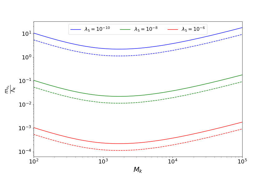
Figure 11: Plot of $m_{\nu_{k}}/\Lambda_{k}$ for $k=1$ (dashed lines), $k=3$ (solid lines) and $m_{R}=805$ GeV.

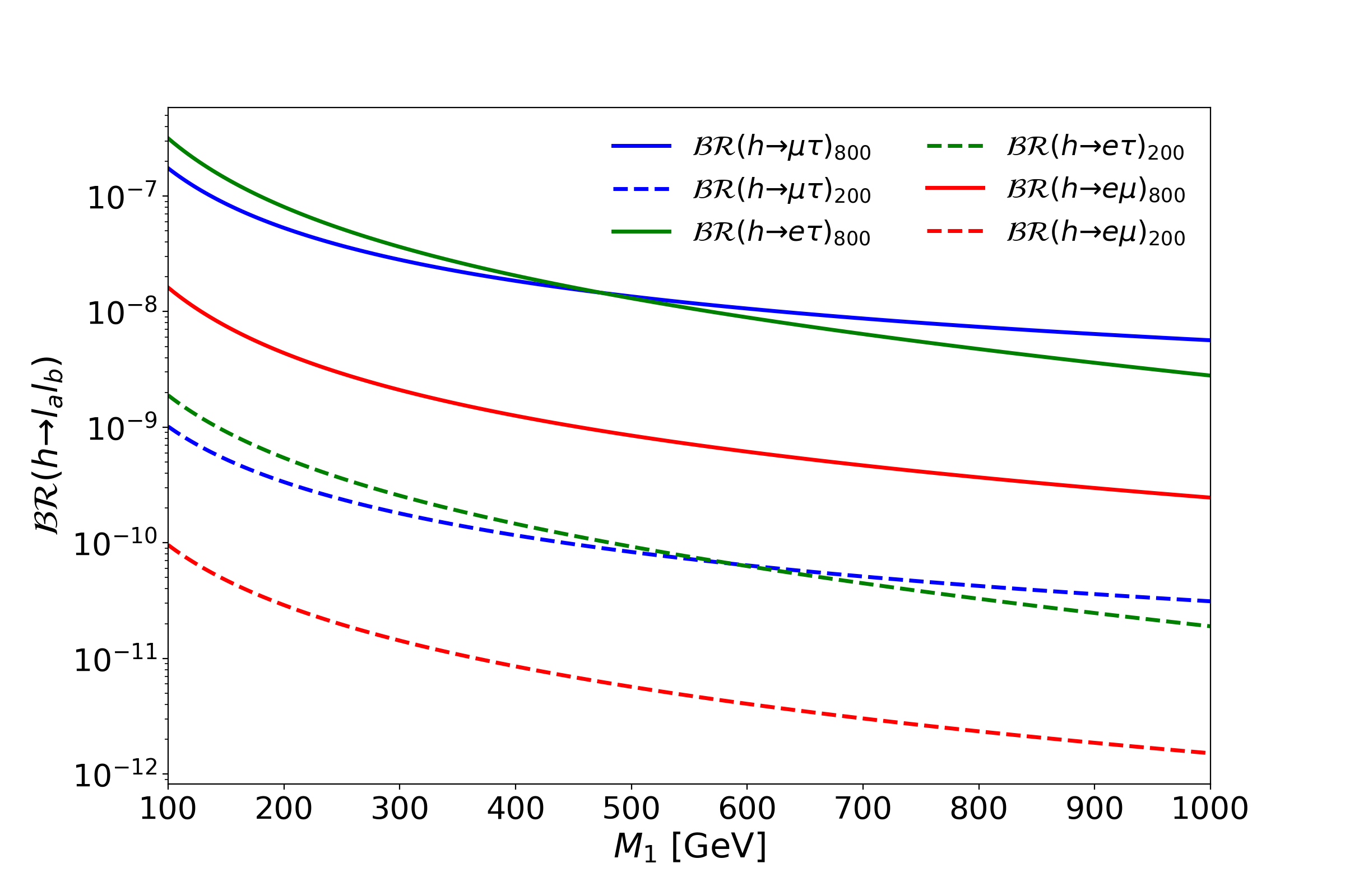
Figure 12: Numerical results for ${\mathcal{BR}}(h\rightarrow l_{a}l_{b})$ vs $M_{1}$ in the Scotogenic model for $M_{2}=10^{4}$ GeV and $M_{3}=10^{5}$ GeV, $\lambda_{5}=1\times 10^{-10}$, $\mu_{2}=1$ GeV. The plot shows two cases: $(i)$ ${\mathcal{BR}}(h\to l_{a}l_{b})_{800}$ with $m_{\eta}=800$ GeV and $m_{R}=805$ GeV (solid lines); $(ii)$ ${\mathcal{BR}}(h\to l_{a}l_{b})_{200}$ with $m_{\eta}=200$ GeV and $m_{R}=205$ GeV (dashed lines).

Figure 12 shows the $\mathcal{BR}(h\to l_{a}l_{b})$ for the Scotogenic model for two scenarios: $(i)$ for $m_{\eta}=800$ GeV, $m_{R}=805$ GeV (solid lines); and $(ii)$ for $m_{\eta}=200$ GeV, $m_{R}=205$ GeV (dashed lines). The largest values of $\mathcal{BR}(h\to l_{a}l_{b})$ are reached for $M_{1}=100$ GeV, which are: $\mathcal{BR}(h\to\mu\tau)_{800}\approx\mathcal{BR}(h\to e\tau)_{800}\approx 10^{-7}$ and $\mathcal{BR}(h\to e\mu)_{800}\approx 10^{-8}$, also $\mathcal{BR}(h\to\mu\tau)_{200}\approx\mathcal{BR}(h\to e\tau)_{200}\approx 10^{-9}$ and $\mathcal{BR}(h\to e\mu)_{200}\approx 10^{-10}$.

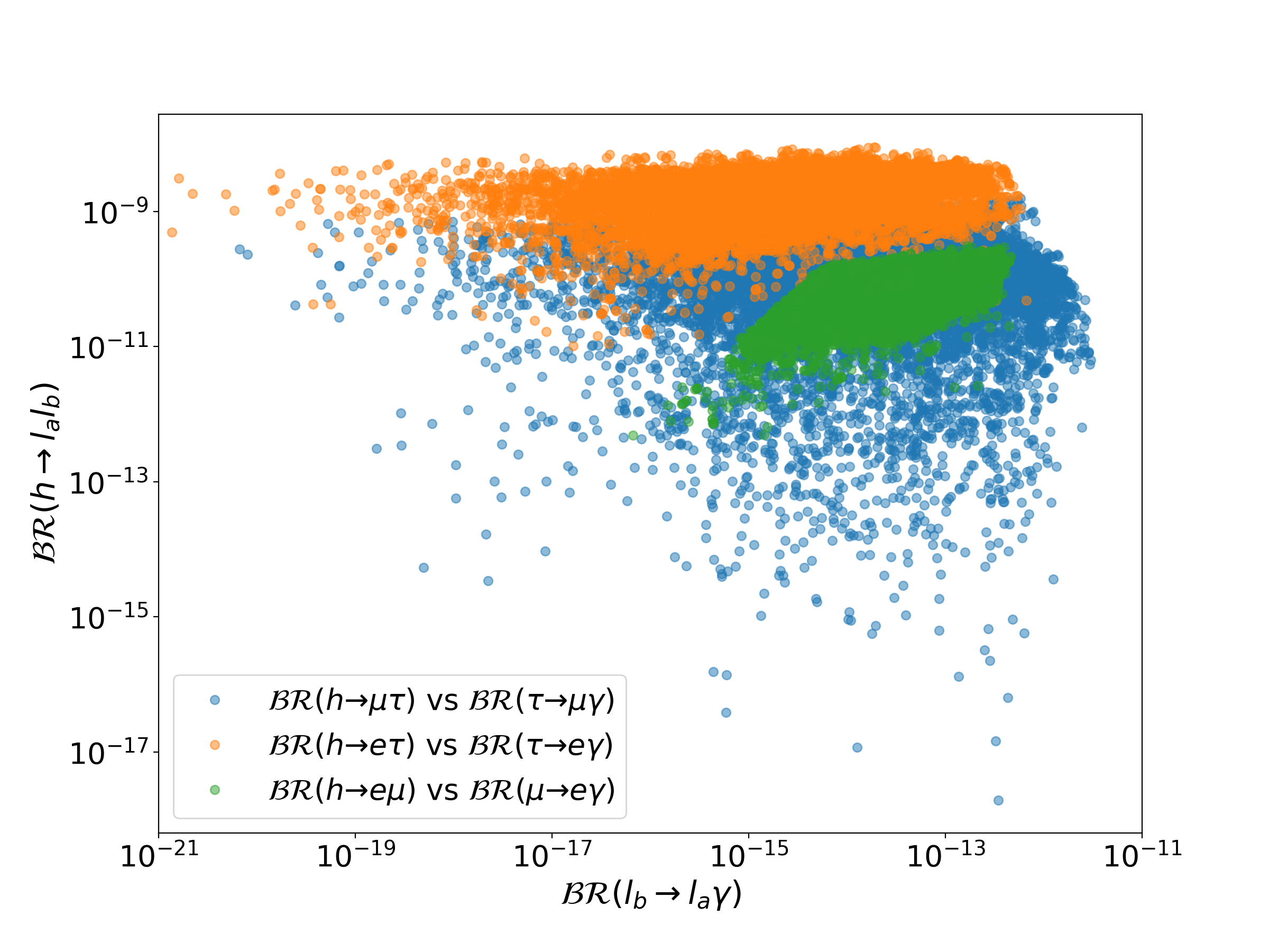
Figure 13: Comparison of $\mathcal{BR}(h\rightarrow l_{a}l_{b})$ and $\mathcal{BR}(l_{b}\rightarrow l_{a}\gamma)$ in the allowed space in the Scotogenic model.

In Ref. Herrero-García et al. (2016) they found that ${\mathcal{BR}}(h\to\mu\tau)\lessapprox 10^{-7}\lambda_{3}^{2}$. In this work we write $\lambda_{3}=\frac{2}{v^{2}}(m_{\eta}^{2}-\mu_{2}^{2})$ in terms of $m_{\eta}\approx 10^{2}$ GeV and $\mu_{2}=1$ GeV. Then by means of equation (42), the corresponding bound of Herrero-García et al. (2016) will be given by ${\mathcal{BR}}(h\to\mu\tau)\lessapprox 10^{-7}$, which is in agreement with our results. Recently, the work Hundi (2022) attempted to find a enhance in LFV Higgs decays signals in the Scotogenic model, they assume $\lambda_{3}\approx 1$, and $\lambda_{5}<<1$ which implies $Y_{{ab}}\approx 1$. In our scan, we obtain $m_{\eta}\approx 10^{2}$ and $\lambda_{5}\approx 10^{-10}$ which implies $\lambda_{3}\approx 1$ and $Y_{{ab}}\approx 1$, naturally, we also agree with these results.

Finally, we have previously analyzed the consequences of electroweak parameters, CLFV process and relic density of dark matter bounds over the parameter space. However, we found that $\mathcal{BR}(h\rightarrow l_{a}l_{b})\lesssim 10^{-9}$, as it is shown in Figure 13. These results satisfy the limits reported by ATLAS and BABAR given in Table 6.

V Conclusions

In this paper we have studied the general formulae for the calculation of one-loop LFV Higgs decays $H_{r}\to l_{a}l_{b}$, with $H_{r}$ being part of the Higgs spectrum of a multi-scalar extension of the SM that includes neutrino masses. In particular, we calculated the form factors for all diagrams that contribute to the LFV Higgs decays, where FCNC are forbidden at tree level; the structure of these diagrams depend on the number of fermions inside the loop. The results calculated in Section II have been implemented in the code named OneLoopLFVHD through the Python library for symbolic calculations Sympy, which enhances its usefulness in the Jupyter notebook graphical interface. With the help of mpmath the symbolic expressions can be implemented numerically with arbitrary precision. The code and examples can be downloaded in the GitHub repository OneLoopLFVHD.

Then, we applied our general formulae for two particular models, and we found agreement for See-Saw Type I-$\nu SM$ with the results given in Pilaftsis (1992); Körner et al. (1993); Arganda et al. (2005); Thao et al. (2017). Finally, for this model, we found that the largest values are $\mathcal{BR}(h\to\mu\tau)\simeq 10^{-12}$ for $m_{n_{6}}\approx 10^{15}$ GeV.

In the case of the Scotogenic model, we found a region of parameter space that satisfies all the constraints from LFV process, dark matter relic density, electroweak precision tests and perturvativity. For LFV Higgs decays, we separate the contributions of heavy and light neutrinos, and we found that the largest contributions come from the heavy neutrinos and light neutrino contribution is negligible. We identify an upper bound on the branching ratios of the order $\mathcal{BR}(h\to l_{a}l_{b})\lesssim 10^{-9}$ for the Scotogenic model. On the other hand, for the heavier Higgs bosons, the corresponding branching ratio could reach much larger values; but we shall present these results elsewhere.

Acknowledgments

M. Z. M. thanks to Conacyt (Mexico) for the PhD fellowship. J. L. D. C. and O. F. B. thank the support of SNI (Mexico).

Appendix A Generic Feynman Rules

The Feynman rules for the models under consideration, have a common structure, as given in Figures 14 and 15. First, we have the scalar, fermionic and vector interactions with $H_{r}$ as it is shown in Figure 14.

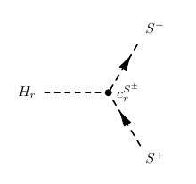
(a) Interaction $H_{r}S^{-}S^{+}$

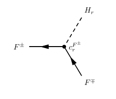
(b) Interaction $H_{r}F^{\pm}F^{\mp}$

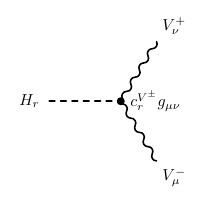
(c) Interaction $H_{r}V^{+}V^{-}$

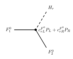
(d) Interaction $H_{r}F_{1}^{0}F_{2}^{0}$

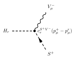
(e) Interaction $H_{r}V^{-}S^{+}$

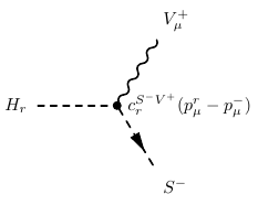
(f) Interaction $H_{r}V^{+}S^{-}$

Figure 14: Feynman rules for scalar, fermionic and vector interactions for $H_{r}$.

For models where FCNC are forbidden at tree level, LFV process are at loop-level mediated only by charged currents either fermionic or bosonic. The generic Feynman rules for these interactions are given in Figure 15.

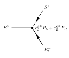
(a) Interaction $S^{+}F_{1}^{0}F_{2}^{-}$

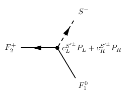
(b) Interaction $S^{-}F_{1}^{0}F_{2}^{+}$

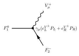
(c) Interaction $V^{+}F_{1}^{0}F_{2}^{-}$

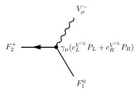
(d) Interaction $V^{-}F_{1}^{0}F_{2}^{+}$

Figure 15: Feynman rules for charged current interactions mediated by charged scalars and vectors.

Appendix B Loop formulae and identities

We use the conventions given in Hue et al. (2016); Thao et al. (2017) for the Passarino-Veltman functions, and using those mass assignments shown in Figure 1, denominators of propagators are given by

$$\operatorname{D}_{0}=k^{2}-M_{0}^{2}+i\delta,\quad\operatorname{D}_{1}=(k-p_{1})^{2}-M_{1}^{2}+i\delta,\quad\operatorname{D}_{2}=(k+p_{2})^{2}-M_{2}^{2}+i\delta,$$ (59)

where $\delta$ is an infinitesimal parameter that allows to perform the loop integrals correctly; $M_{i}$ denotes the mass of particle $P_{i}$ inside the loop, with $p_{1}$, $p_{2}$ denoting the lepton momentum $l_{a}$, $l_{b}$, respectively.

We use dimensional regularization, where the four dimensional momentum integral can be rewritten as

$$\int\frac{d^{4}k}{(2\pi)^{4}}\rightarrow\frac{i}{16\pi^{2}}\times\frac{(2\pi\mu)^{4-D}}{i\pi^{2}}\int d^{4}k,$$ (60)

where $\mu$ is a parameter with mass dimensions. Following the conventions of Hue et al. (2016), this step will be omitted, the final results will be obtained by including the factor $i/16\pi^{2}$.

In the Feynman gauge, only the following scalar integrals are present:

$$\operatorname{B}_{0}^{(i)}(M_{0},M_{i})=N_{D}\int\frac{d^{D}k}{\operatorname{D}_{0}\operatorname{D}_{i}}, \operatorname{B}_{0}^{(12)}(M_{1},M_{2})=N_{D}\int\frac{d^{D}k}{\operatorname{D}_{1}\operatorname{D}_{2}},$$ (61a)

$$\operatorname{C}_{0}(M_{0},M_{1},M_{2})=\frac{1}{i\pi^{2}}\int\frac{d^{4}k}{\operatorname{D}_{0}\operatorname{D}_{1}\operatorname{D}_{2}},$$ (61b)

where $N_{D}=(2\pi\mu)^{4-D}/i\pi^{2}$ and $D=4-2\epsilon$. The tensor integrals are the following

$$\operatorname{B}^{\mu}(p_{i},M_{0},M_{i}) =N_{D}\int\frac{d^{D}k\times k^{\mu}}{D_{0}D_{i}}=\operatorname{B}_{1}^{(i)}p_{i}^{\mu},$$ (62a)

$$\operatorname{C}^{\mu}=\operatorname{C}^{\mu}(M_{0},M_{1},M_{2}) =\frac{1}{i\pi^{2}}\int\frac{d^{4}k\times k^{\mu}}{D_{0}D_{1}D_{2}}=\operatorname{C}_{1}p_{1}^{\mu}+\operatorname{C}_{2}p_{2}^{\mu}.$$ (62b)

On the other hand, we know that $\operatorname{C}_{i}$ ($i=0,1,2$) integrals are finite, but the $\operatorname{B}$ functions contain divergences. The divergent integrals are written in terms of its divergent and finite terms (denoted by the lowercase):

$$\operatorname{B}_{0,1}^{(i)} =Div[\operatorname{B}_{0,1}^{(i)}]+b_{0,1}^{(i)},$$ (63a)

$$\operatorname{B}_{0}^{(12)} =Div[\operatorname{B}_{0}^{(12)}]+b_{0}^{(12)}.$$ (63b)

Also,

$$Div[\operatorname{B}_{0}^{(i)}] =Div[\operatorname{B}_{0}^{(12)}]=\Delta_{\epsilon},$$ (64a)

$$Div[\operatorname{B}_{1}^{(1)}] =-Div[\operatorname{B}_{1}^{(2)}]=\frac{1}{2}\Delta_{\epsilon},$$ (64b)

where $\Delta_{\epsilon}=1/\epsilon+\ln{4\pi}-\gamma_{E}+\ln{\frac{\mu^{2}}{m_{r}^{2}}}$ with $\gamma_{E}$ the Euler constant, and $m_{r}$ is the mass $H_{r}$. For simplicity in calculation, we use approximate expressions for PV functions, where $p_{1}^{2},\,p_{2}^{2}\to 0$. The $\operatorname{C}_{0}$ function is given by Hue et al. (2016); Bardin and Passarino (1999):

$$\operatorname{C}_{0}=\frac{1}{m_{r}^{2}}\left[R_{0}\left(x_{0},x_{1}\right)+R_{0}\left(x_{0},x_{2}\right)-R_{0}\left(x_{0},x_{3}\right)\right],$$ (65)

where

$$R_{0}\left(x_{0},x_{i}\right)\equiv Li_{2}\left(\frac{x_{0}}{x_{0}-x_{i}}\right)-Li_{2}\left(\frac{x_{0}-1}{x_{0}-x_{i}}\right),$$ (66)

with $Li_{2}$ the dilogarithm function. Also,

$$x_{0}=\frac{M_{2}^{2}-M_{0}^{2}}{m_{r}^{2}},\quad x_{3}=\frac{-M_{0}^{2}+i\delta}{M_{1}^{2}-M_{0}^{2}},$$ (67)

and the $x_{1,2}$ are solutions of

$$x^{2}-\left(\frac{m_{r}^{2}-M_{1}^{2}+M_{2}^{2}}{m_{r}^{2}}\right)x+\frac{M_{2}^{2}-i\delta}{m_{r}^{2}}=0.$$ (68)

The finite part of $\operatorname{B}^{(i)}_{0,1}$ functions can be evaluated in a numerically stable way using Denner and Dittmaier (2006)

$$b_{0}^{(i)} =-\ln{M_{0}^{2}}-\sum_{l=1}^{2}f_{0}\left(y_{kl}\right),\,$$ (69a)

$$b_{1}^{(i)} =(-1)^{i-1}\frac{1}{2}\left(-\ln{M_{0}^{2}}-\sum_{l=1}^{2}f_{1}\left(y_{kl}\right)\right),$$ (69b)

where $y_{kl}$ with $k=i,j$, $l=1,2$ are solutions of

$$y^{2}p_{i}^{2}-y(p_{i}^{2}+M_{0}^{2}-M_{1}^{2})+M_{0}^{2}-i\delta =0,$$ (70a)

$$y^{2}p_{j}^{2}-y(p_{j}^{2}+M_{0}^{2}-M_{2}^{2})+M_{0}^{2}-i\delta =0,$$ (70b)

and are given by

$$y_{i} =\frac{1}{2p_{i}^{2}}\left[p_{i}^{2}+M_{0}^{2}-M_{1}^{2}\pm\sqrt{(p_{i}^{2}+M_{0}^{2}-M_{1}^{2})^{2}-4p_{i}^{2}M_{0}^{2}}\right],$$ (71a)

$$y_{j} =\frac{1}{2p_{j}^{2}}\left[p_{j}^{2}+M_{0}^{2}-M_{2}^{2}\pm\sqrt{(p_{j}^{2}+M_{0}^{2}-M_{2}^{2})^{2}-4p_{j}^{2}M_{0}^{2}}\right].$$ (71b)

Also,

$$f_{0}(y) =y\ln(-y)-y\ln(1-y)+\ln(1-\frac{1}{y})-1$$ (72a)

$$f_{1}(y) =y^{2}\ln(-y)-y^{2}\ln(1-y)-y+\ln(1-\frac{1}{y})-\frac{1}{2},$$ (72b)

derived from

$$f_{n}(x)\equiv(n+1)\int_{0}^{1}\mathrm{~{}d}t\,t^{n}\ln\left(1-\frac{t}{x}\right).$$ (73)

These functions have poles in $y=0,1$.

The expressions for $b_{0}^{(12)}$ and $\operatorname{C}_{i}$ are as follows Thao et al. (2017)

$$b_{0}^{(12)} =-\ln{M_{1}^{2}}+2+\sum_{k=1}^{2}x_{k}\ln{\left(1-\frac{1}{x_{k}}\right)},$$ (74a)

$$\operatorname{C}_{1} =\frac{1}{m_{r}^{2}}\left[b_{0}^{(1)}-b_{0}^{(12)}+(M_{2}^{2}-M_{0}^{2})\operatorname{C}_{0}\right],$$ (74b)

$$\operatorname{C}_{2} =-\frac{1}{m_{r}^{2}}\left[b_{0}^{(2)}-b_{0}^{(12)}+(M_{1}^{2}-M_{0}^{2})\operatorname{C}_{0}\right],$$ (74c)

where $b_{0}^{(12)}$ depends on $x_{k}$, which are solutions of equation (68). If we focus on the definition of $b_{0}^{(12)}$, we observe that this definition has poles when $x_{k}=0,1$. From equation (68), $x_{k}=x_{k}(M_{1},M_{2},m_{r})$ and we can deduce the following limit cases:

$$x_{1,2} =1\text{ for }M_{1} =0\text{ and }M_{2}=m_{r},$$ (75a)

$$x_{1,2} =0\text{ for }M_{1} =m_{r}\text{ and }M_{2}=0.$$ (75b)

The expressions (65) and (74) have been taken from Hue et al. (2016) and numerically evaluated, the results are compared with LoopTools Phan et al. (2016) finding a good agreement.

Appendix C Cancellation of divergences in the $\nu$SM

It follows from equations (13) and  (14) that

$$M_{ab}^{\nu}=0, \quad M_{(I+3)(J+3)}^{\nu}=\left(M_{N}\right)_{IJ},\quad M_{a(I+3)}^{\nu}=\left(M_{D}\right)_{aI},\quad M_{(I+3)a}^{\nu}=\left(M_{D}^{T}\right)_{Ia},$$ (76)

$$\mathbf{U}^{\nu\dagger}\mathbf{U}^{\nu}=\mathbf{I}, \quad\mathbf{M}^{\nu}=\mathbf{U}^{\nu*}\hat{\mathbf{M}}^{\nu}\mathbf{U}^{\nu\dagger},\quad\text{and}\quad\mathbf{M}^{\nu*}=\mathbf{U}^{\nu}\hat{\mathbf{M}}^{\nu}\mathbf{U}^{\nu T}.$$

These relations will be useful in the cancellation of divergences form the form factors. In particular, to analyze the divergent terms we focus forts for the $R$-form factors $A_{R}$, while those of the $L$-factors can be done along the same lines. All diagrams in the $\nu$SM are given in Table 3, we focus only on diagrams 1, 7, 8, 9 and 10, which contain divergent terms.

Let us start with the divergences for diagram 1 given by

$$Div\left[A_{R}^{(1)}\right] ={m}_{b}\sum_{i,j=1}^{6}\left[\Delta_{\epsilon}m_{n_{i}}^{2}{{{C}}}_{ij}+\Delta_{\epsilon}m_{n_{i}}m_{n_{j}}C^{*}_{ij}\right]\Delta_{ij}^{ab}$$

$$={m}_{b}\sum_{i,j=1}^{6}\left[\Delta_{\epsilon}m_{n_{i}}^{2}{{{C}}}_{ij}\right]\Delta_{ij}^{ab}.$$

Note that in second line, we have considered

$$\sum_{i,j=1}^{6}m_{n_{i}}m_{n_{j}}C^{*}_{ij}\Delta_{ij}^{ab} =\frac{g^{3}}{64\pi^{2}m_{W}^{3}}\sum_{i,j=1}^{6}\sum_{c=1}^{3}m_{n_{i}}m_{n_{j}}U_{ci}^{\nu*}U_{cj}^{\nu}U_{bj}^{\nu}U_{ai}^{\nu*}$$

$$=\frac{g^{3}}{64\pi^{2}m_{W}^{3}}\sum_{j=1}^{6}\sum_{c=1}^{3}m_{n_{j}}U_{bj}^{\nu}U_{cj}^{\nu}\sum_{i=1}^{6}m_{n_{i}}U_{ci}^{\nu*}U_{ai}^{\nu*}$$

$$=\frac{g^{3}}{64\pi^{2}m_{W}^{3}}\sum_{j=1}^{6}\sum_{c=1}^{3}m_{n_{j}}U_{bj}^{\nu}U_{cj}^{\nu}(U^{\nu*}\hat{M}_{\nu},U^{\nu\dagger})_{ac}=0,$$ (77)

and definitions of $C_{ij}$ and $\Delta_{ij}^{ab}$ (18). On the other hand,

$$\sum_{i,j=1}^{6}m_{n_{i}}^{2}{C}_{ij}\Delta_{ij}^{ab} =\frac{g^{3}}{64\pi^{2}m_{W}^{3}}\sum_{i,j=1}^{6}\sum_{c=1}^{3}m_{n_{i}}^{2}U_{ci}^{\nu}U_{cj}^{\nu*}U_{bj}^{\nu}U_{ai}^{\nu*}$$

$$=\frac{g^{3}}{64\pi^{2}m_{W}^{3}}\sum_{i=1}^{6}\sum_{c=1}^{3}m_{n_{i}}^{2}U_{ci}^{\nu}U_{ai}^{\nu*}\sum_{j=1}^{6}U_{bj}^{\nu}U_{cj}^{\nu*}$$

$$=\frac{g^{3}}{64\pi^{2}m_{W}^{3}}\sum_{i=1}^{6}\sum_{c=1}^{3}m_{n_{i}}^{2}U_{ci}^{\nu}U_{ai}^{\nu*}(U^{\nu}U^{\nu\dagger})_{bc}$$

$$=\sum_{i=1}^{6}m_{n_{i}}^{2}\Delta_{ii}^{ab},$$ (78)

where unitarity of $U^{\nu}$ has been used. Considering equations (77) and (78), the divergent term of $A_{R}^{(1)}$ is

$$Div\left[A_{R}^{(1)}\right] ={m}_{b}\Delta_{\epsilon}\sum_{i=1}^{6}m_{n_{i}}^{2}\Delta_{ii}^{ab}.$$

Now, consider the diagrams 8 and 10, its right divergent terms are given by

$$Div\left[A_{R}^{(8)}\right] =\frac{{m}_{b}}{{m}_{a}^{2}-{m}_{b}^{2}}\sum_{i=1}^{6}\left(m_{n_{i}}^{2}\left({m}_{a}^{2}+{m}_{b}^{2}\right)\Delta_{\epsilon}-m_{a}^{2}\left({m}_{b}^{2}+m_{n_{i}}^{2}\right)\frac{\Delta_{\epsilon}}{2}\right)\Delta_{ii}^{ab}$$

$$=\frac{{m}_{b}}{{m}_{a}^{2}-{m}_{b}^{2}}\sum_{i=1}^{6}\left(\frac{\Delta_{\epsilon}}{2}m_{n_{i}}^{2}m_{a}^{2}+m_{b}^{2}\Delta_{\epsilon}\left(m_{n_{i}}^{2}-\frac{m_{a}^{2}}{2}\right)\right)\Delta_{ii}^{ab},$$ (79)

$$Div\left[A_{R}^{(10)}\right] =-\frac{{m}_{a}^{2}m_{b}}{{m}_{a}^{2}-{m}_{b}^{2}}\sum_{i=1}^{6}\left(\left({m}_{b}^{2}+m_{n_{i}}^{2}\right)\left(-\frac{\Delta_{\epsilon}}{2}\right)+2\Delta_{\epsilon}m_{n_{i}}^{2}\right)\Delta_{ii}^{ab}$$

$$=-\frac{{m}_{a}^{2}m_{b}}{{m}_{a}^{2}-{m}_{b}^{2}}\sum_{i=1}^{6}\left(\frac{3\Delta_{\epsilon}}{2}m_{n_{i}}^{2}-m_{b}^{2}\frac{\Delta_{\epsilon}}{2}\right)\Delta_{ii}^{ab}.$$ (80)

After some simplifications we obtain

$$Div\left[A_{R}^{(8)}\right]+Div\left[A_{R}^{(10)}\right]=-{m}_{b}\Delta_{\epsilon}\sum_{i=1}^{6}m_{n_{i}}^{2}\Delta_{ii}^{ab},$$

then divergent terms of diagrams 1, 8 and 10 disappear when we sum each other.

In the case of diagrams 7 and 9 we have the next divergent terms

$$Div\left[A_{R}^{(7)}\right] =-\frac{2m_{W}^{2}{m}_{a}^{2}{m}_{b}}{{m}_{a}^{2}-{m}_{b}^{2}}\sum_{i=1}^{6}\frac{\Delta_{\epsilon}}{2}\Delta_{ii}^{ab},$$ (81)

$$Div\left[A_{R}^{(9)}\right] =-\frac{2m_{W}^{2}{m}_{a}^{2}{m}_{b}}{{m}_{a}^{2}-{m}_{b}^{2}}\sum_{i=1}^{6}\left(-\frac{\Delta_{\epsilon}}{2}\right)\Delta_{ii}^{ab},$$ (82)

but each of them is null by the GIM mechanism.

References

- Zyla et al. [2020] P. Zyla et al. (Particle Data Group), PTEP 2020, 083C01 (2020).
- Chatrchyan et al. [2012] S. Chatrchyan et al. (CMS), Phys. Lett. B 716, 30 (2012), eprint 1207.7235.
- Aad et al. [2012] G. Aad et al. (ATLAS), Phys. Lett. B 716, 1 (2012), eprint 1207.7214.
- Ellis and You [2012] J. Ellis and T. You, Journal of High Energy Physics 2012, 140 (2012), ISSN 1029-8479, URL https://doi.org/10.1007/JHEP06(2012)140.
- Ellis [2012] J. Ellis, Philosophical Transactions of the Royal Society A: Mathematical, Physical and Engineering Sciences 370, 818 (2012), eprint https://royalsocietypublishing.org/doi/pdf/10.1098/rsta.2011.0452, URL https://royalsocietypublishing.org/doi/abs/10.1098/rsta.2011.0452.
- Wan and Wang [2020] Z. Wan and J. Wang, Journal of High Energy Physics 2020, 62 (2020), ISSN 1029-8479, URL https://doi.org/10.1007/JHEP07(2020)062.
- Bertone et al. [2005] G. Bertone, D. Hooper, and J. Silk, Phys. Rept. 405, 279 (2005), eprint hep-ph/0404175.
- Lorenzo Diaz-Cruz [2019] J. Lorenzo Diaz-Cruz, Rev. Mex. Fis. 65, 419 (2019), eprint 1904.06878.
- Ho and Tandean [2013a] S.-Y. Ho and J. Tandean, Physical Review D 87 (2013a), ISSN 1550-2368, URL http://dx.doi.org/10.1103/PhysRevD.87.095015.
- Roig [2016] P. Roig, Lepton flavor violation in the simplest little higgs model (2016), eprint 1610.01266.
- Poh and Raby [2017] Z. Poh and S. Raby, Physical Review D 96 (2017), ISSN 2470-0029, URL http://dx.doi.org/10.1103/PhysRevD.96.015032.
- Boyarkin et al. [2018] O. M. Boyarkin, G. G. Boyarkina, and D. S. Vasileuskaya, International Journal of Modern Physics A 33, 1850103 (2018), ISSN 1793-656X, URL http://dx.doi.org/10.1142/S0217751X18501038.
- Arroyo-Urea and Diaz-Cruz [2020] M. A. Arroyo-Urea and J. L. Diaz-Cruz, Phys. Lett. B810, 135799 (2020), eprint 2005.01153.
- Aad et al. [2020] G. Aad et al. (ATLAS), Phys. Lett. B 800, 135069 (2020), eprint 1907.06131.
- Savina [2021] M. Savina (ATLAS, CMS), PoS LHCP2020, 176 (2021).
- Diaz et al. [2003] R. A. Diaz, R. Martinez, and J. A. Rodriguez, Phys. Rev. D 67, 075011 (2003), eprint hep-ph/0208117.
- Diaz-Cruz et al. [2005] J. L. Diaz-Cruz, R. Noriega-Papaqui, and A. Rosado, Phys. Rev. D71, 015014 (2005), eprint hep-ph/0410391.
- Primulando et al. [2020a] R. Primulando, J. Julio, and P. Uttayarat, Phys. Rev. D 101, 055021 (2020a), eprint 1912.08533.
- Ghosh and Lahiri [2021] N. Ghosh and J. Lahiri (2021), eprint 2103.10632.
- Diaz-Cruz [2003] J. L. Diaz-Cruz, JHEP 05, 036 (2003), eprint hep-ph/0207030.
- Alvarado et al. [2016] C. Alvarado, R. M. Capdevilla, A. Delgado, and A. Martin, Phys. Rev. D 94, 075010 (2016), eprint 1602.08506.
- Arganda et al. [2005] E. Arganda, A. M. Curiel, M. J. Herrero, and D. Temes, Phys. Rev. D 71, 035011 (2005), URL https://link.aps.org/doi/10.1103/PhysRevD.71.035011.
- Kubo et al. [2006a] J. Kubo, E. Ma, and D. Suematsu, Phys. Lett. B 642, 18 (2006a), eprint hep-ph/0604114.
- Baldini et al. [2016] A. M. Baldini et al. (MEG), Eur. Phys. J. C 76, 434 (2016), eprint 1605.05081.
- Nomura et al. [2021] T. Nomura, H. Okada, and Y. Uesaka, Nucl. Phys. B 962, 115236 (2021), eprint 2008.02673.
- Diaz-Cruz and Toscano [2000] J. L. Diaz-Cruz and J. J. Toscano, Phys. Rev. D62, 116005 (2000), eprint hep-ph/9910233.
- Diaz-Cruz et al. [2004] J. L. Diaz-Cruz, R. Noriega-Papaqui, and A. Rosado, Phys. Rev. D69, 095002 (2004), eprint hep-ph/0401194.
- Herrero et al. [2010] M. Herrero, J. Portoles, and A. Rodriguez-Sanchez, AIP Conf. Proc. 1200, 908 (2010), eprint 0909.0724.
- Herrero et al. [2017] M. J. Herrero, E. Arganda, X. Marcano, R. Morales, and A. Szynkman, PoS EPS-HEP2017, 114 (2017), eprint 1710.02510.
- Barradas-Guevara et al. [2017] E. Barradas-Guevara, J. L. Diaz-Cruz, O. Félix-Beltrán, and U. J. Saldana-Salazar (2017), eprint 1706.00054.
- Arana-Catania et al. [2013] M. Arana-Catania, E. Arganda, and M. J. Herrero, JHEP 09, 160 (2013), [Erratum: JHEP 10, 192 (2015)], eprint 1304.3371.
- Hue et al. [2016] L. T. Hue, H. N. Long, T. T. Thuc, and T. Phong Nguyen, Nucl. Phys. B907, 37 (2016), eprint 1512.03266.
- Thao et al. [2017] N. Thao, L. Hue, H. Hung, and N. Xuan, Nuclear Physics B 921, 159 (2017), ISSN 0550-3213, URL http://www.sciencedirect.com/science/article/pii/S0550321317301785.
- et. al. [2020] G. A. et. al., Physics Letters B 800, 135069 (2020), ISSN 0370-2693, URL http://www.sciencedirect.com/science/article/pii/S0370269319307919.
- Sirunyan et al. [2020] A. M. Sirunyan, A. Tumasyan, W. Adam, F. Ambrogi, T. Bergauer, J. Brandstetter, M. Dragicevic, J. Erö, A. Escalante Del Valle, and et al., Journal of High Energy Physics 2020 (2020), ISSN 1029-8479, URL http://dx.doi.org/10.1007/JHEP03(2020)103.
- Tsumura [2005] K. Tsumura, in Summer Institute 2005 (SI2005) (2005), eprint hep-ph/0511253.
- Kanemura et al. [2006] S. Kanemura, T. Ota, and K. Tsumura, Phys. Rev. D 73, 016006 (2006), URL https://link.aps.org/doi/10.1103/PhysRevD.73.016006.
- Primulando et al. [2020b] R. Primulando, J. Julio, and P. Uttayarat, Physical Review D 101 (2020b), ISSN 2470-0029, URL http://dx.doi.org/10.1103/PhysRevD.101.055021.
- Vicente [2019] A. Vicente, Front. in Phys. 7, 174 (2019), eprint 1908.07759.
- Arroyo-Urea et al. [2018] M. A. Arroyo-Urea, J. L. Diaz-Cruz, G. Tavares-Velasco, A. Bolaos, and G. Hernández-Tomé, Phys. Rev. D98, 015008 (2018), eprint 1801.00839.
- Pilaftsis [1992] A. Pilaftsis, Physics Letters B 285, 68 (1992), ISSN 0370-2693, URL https://www.sciencedirect.com/science/article/pii/037026939291301O.
- Körner et al. [1993] J. G. Körner, A. Pilaftsis, and K. Schilcher, Phys. Rev. D 47, 1080 (1993), URL https://link.aps.org/doi/10.1103/PhysRevD.47.1080.
- Arganda et al. [2015] E. Arganda, M. J. Herrero, X. Marcano, and C. Weiland, Phys. Rev. D 91, 015001 (2015), URL https://link.aps.org/doi/10.1103/PhysRevD.91.015001.
- Hernández-Tomé et al. [2020] G. Hernández-Tomé, J. I. Illana, and M. Masip, Phys. Rev. D 102, 113006 (2020), URL https://link.aps.org/doi/10.1103/PhysRevD.102.113006.
- Brignole and Rossi [2003] A. Brignole and A. Rossi, Physics Letters B 566, 217 (2003), ISSN 0370-2693, URL http://www.sciencedirect.com/science/article/pii/S0370269303008372.
- Diaz-Cruz et al. [2009] J. L. Diaz-Cruz, D. K. Ghosh, and S. Moretti, Phys. Lett. B679, 376 (2009), eprint 0809.5158.
- Arganda et al. [2016] E. Arganda, M. J. Herrero, R. Morales, and A. Szynkman, Journal of High Energy Physics 2016, 55 (2016), ISSN 1029-8479, URL https://doi.org/10.1007/JHEP03(2016)055.
- Arganda et al. [2017] E. Arganda, M. J. Herrero, X. Marcano, R. Morales, and A. Szynkman, Phys. Rev. D 95, 095029 (2017), URL https://link.aps.org/doi/10.1103/PhysRevD.95.095029.
- Marcano and Morales [2020] X. Marcano and R. A. Morales, Frontiers in Physics 7 (2020), ISSN 2296-424X, URL https://www.frontiersin.org/article/10.3389/fphy.2019.00228.
- Coy and Frigerio [2019] R. Coy and M. Frigerio, Phys. Rev. D 99, 095040 (2019), URL https://link.aps.org/doi/10.1103/PhysRevD.99.095040.
- Denner et al. [1992] A. Denner, H. Eck, O. Hahn, and J. Küblbeck, Nuclear Physics B 387, 467 (1992), ISSN 0550-3213, URL https://www.sciencedirect.com/science/article/pii/055032139290169C.
- Phan et al. [2016] K. H. Phan, H. Hung, and L. Hue, Progress of Theoretical and Experimental Physics 2016 (2016), ISSN 2050-3911, 113B03, eprint https://academic.oup.com/ptep/article-pdf/2016/11/113B03/9621072/ptw158.pdf, URL https://doi.org/10.1093/ptep/ptw158.
- Johansson et al. [2013] F. Johansson et al., mpmath: a Python library for arbitrary-precision floating-point arithmetic (version 0.18) (2013), http://mpmath.org/.
- Ilakovac and Pilaftsis [1995] A. Ilakovac and A. Pilaftsis, Nuclear Physics B 437, 491 (1995), ISSN 0550-3213, URL https://www.sciencedirect.com/science/article/pii/055032139400567X.
- Marcano Imaz [2017] X. Marcano Imaz, Lepton flavor violation from low scale seesaw neutrinos with masses reachable at the LHC (2017), eprint 1710.08032.
- Esteban et al. [2019] I. Esteban, M. C. Gonzalez-Garcia, A. Hernandez-Cabezudo, M. Maltoni, and T. Schwetz, JHEP 01, 106 (2019), eprint 1811.05487.
- Aghanim et al. [2018] N. Aghanim et al. (Planck) (2018), eprint 1807.06209.
- Casas and Ibarra [2001] J. Casas and A. Ibarra, Nuclear Physics B 618, 171 (2001), ISSN 0550-3213, URL http://www.sciencedirect.com/science/article/pii/S0550321301004758.
- Ma [2006] E. Ma, Phys. Rev. D 73, 077301 (2006), URL https://link.aps.org/doi/10.1103/PhysRevD.73.077301.
- Herrero-García et al. [2016] J. Herrero-García, N. Rius, and A. Santamaria, Journal of High Energy Physics 2016, 84 (2016), ISSN 1029-8479, URL https://doi.org/10.1007/JHEP11(2016)084.
- Hundi [2022] R. S. Hundi, Eur. Phys. J. C 82, 505 (2022), eprint 2201.03779.
- Grimus et al. [2008] W. Grimus, L. Lavoura, O. Ogreid, and P. Osland, Nuclear Physics B 801, 81 (2008), ISSN 0550-3213, URL http://www.sciencedirect.com/science/article/pii/S0550321308002289.
- Aubert et al. [2010] B. Aubert et al. (BaBar), Phys. Rev. Lett. 104, 021802 (2010), eprint 0908.2381.
- Uno et al. [2021] K. Uno, K. Hayasaka, K. Inami, I. Adachi, H. Aihara, D. M. Asner, H. Atmacan, T. Aushev, R. Ayad, V. Babu, et al., Journal of High Energy Physics 2021, 19 (2021), ISSN 1029-8479, URL https://doi.org/10.1007/JHEP10(2021)019.
- Toma and Vicente [2014] T. Toma and A. Vicente, Journal of High Energy Physics 2014, 160 (2014), ISSN 1029-8479, URL https://doi.org/10.1007/JHEP01(2014)160.
- Ho and Tandean [2013b] S.-Y. Ho and J. Tandean, Phys. Rev. D 87, 095015 (2013b), URL https://link.aps.org/doi/10.1103/PhysRevD.87.095015.
- Kubo et al. [2006b] J. Kubo, E. Ma, and D. Suematsu, Physics Letters B 642, 18 (2006b), ISSN 0370-2693, URL http://www.sciencedirect.com/science/article/pii/S037026930601094X.
- Jungman et al. [1996] G. Jungman, M. Kamionkowski, and K. Griest, Physics Reports 267, 195 (1996), ISSN 0370-1573, URL http://www.sciencedirect.com/science/article/pii/0370157395000585.
- Staub [2014] F. Staub, Computer Physics Communications 185, 1773 (2014), ISSN 0010-4655, URL http://www.sciencedirect.com/science/article/pii/S0010465514000629.
- Bardin and Passarino [1999] D. Y. Bardin and G. Passarino, The standard model in the making: Precision study of the electroweak interactions (1999).
- Denner and Dittmaier [2006] A. Denner and S. Dittmaier, Nuclear Physics B 734, 62 (2006), ISSN 0550-3213, URL https://www.sciencedirect.com/science/article/pii/S0550321305009788.