Small Obstacle in a Large Polar Flock

Abstract

We show that arbitrarily large polar flocks are susceptible to the presence of a single small obstacle. In a wide region of parameter space, the obstacle triggers counter-propagating dense bands leading to reversals of the flow. In very large systems, these bands interact yielding a never-ending chaotic dynamics that constitutes a new disordered phase of the system. While most of these results were obtained using simulations of aligning self-propelled particles, we find similar phenomena at the continuous level, not when considering the basic Toner-Tu hydrodynamic theory, but in simulations of truncations of the relevant Boltzmann equation.

In numerical and theoretical studies of active matter, ‘polar flocks’ continue to play a central role (see, e.g. Souslov et al. (2017); Martín-Gómez et al. (2018); Kourbane-Houssene et al. (2018); Geyer et al. (2019); Mahault et al. (2019); Sone and Ashida (2019); Dadhichi et al. (2020); Tasaki (2020); Martin et al. (2021); James et al. (2021); Sesé-Sansa et al. (2021); Zhao et al. (2021); Duan et al. (2021) for recent examples). This term refers to the homogeneous collective motion, resulting from spontaneous rotational symmetry breaking, of self-propelled particles locally aligning their velocities, as in the Vicsek model Vicsek et al. (1995); Ginelli (2016); Chaté (2020). Remarkably, polar flocks exhibit true long-range polar order even in two space dimensions (2D), as argued by Toner and Tu, who also predicted the scaling structure of their space-time fluctuations Toner and Tu (1995, 1998); Toner (2012); Mahault et al. (2019). Since these early works, a wealth of results have been obtained on particle-level models, hydrodynamic theories, and even experimental realizations of polar flocks Deseigne et al. (2010); Weber et al. (2013); Kumar et al. (2013); Soni et al. (2020); Geyer et al. (2018); Iwasawa et al. (2021). The overall phase diagram of such dry aligning dilute active matter is best described as resulting from a phase-separation scenario in which homogeneous polar flocks form an orientationally-ordered liquid separated from a disordered gas by a coexistence phase involving dense and ordered travelings bands Solon et al. (2015); Chaté and Mahault (2021); Chaté (2020). This has been recently shown to hold even in the case of non-metric, ‘topological’ interactions, a case that was heretofore believed to show a direct order-disorder transition Martin et al. (2021).

Polar flocks are thus observed in a rather large class of active matter systems and there is evidence of the robustness of their properties. But there are also clear indications of their fragility. For instance even weakly non-reciprocal interactions have been shown to substantially modify phase diagrams Chen et al. (2017); Dadhichi et al. (2020); Fruchart et al. (2021). Further evidence is found in recent works that demonstrated a variety of effects induced by spatial quenched disorder Chepizhko et al. (2013); Toner et al. (2018a, b); Duan et al. (2021); Chardac et al. (2021). The Toner-Tu long-range polar order has been argued to be qualitatively changed for flocks moving on disordered substrates. It has been shown that different types of quenched disorder can have different effects. In most cases, arbitrarily weak disorder modifies or breaks long-range polar order.

The above cases of quenched disorder include that of scattered small obstacles, which was considered in models and in experiments Chepizhko et al. (2013); Chardac et al. (2021). But what about the effect of a single obstacle? The insertion of passive objects in a disordered gas of active particles is known to have non-trivial consequences, introducing in particular long-range currents in the active gas Baek et al. (2018); Granek et al. (2020); Rohwer et al. (2020); Knežević and Stark (2020); Liu et al. (2020); Sebtosheikh and Naji (2020); Speck and Jayaram (2021). Given this, one can expect that even a single passive obstacle introduced within a long-range correlated polar flock may have major consequences on the large-scale dynamics of the system.

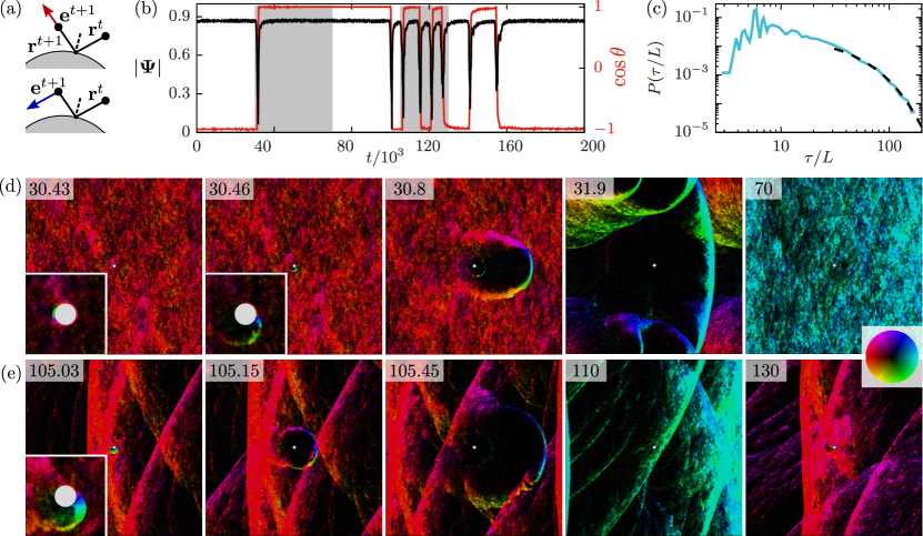
Figure 1: Typical flow reversals in a system of size $L=1024$ at $\eta=0.5$ with $\sigma=22$. (a) Sketch of collision rules: Orientation is either reflected (type 1, in red) or kept (type 2, in blue). (b) Time series of the global polarization $|\bm{\Psi}|$, in black, and its orientation $\cos\theta$, in red. Shaded regions indicate the time windows for the snapshots series in (d), and (e). (c) Distribution of Inter-reversal times $P(\tau)$. Dashed line indicates an exponential decay. (d) Snapshots of the system during an isolated reversal, and its recovery. On the color wheel on the right, color and intensity represent, respectively, the angle of the locally averaged polarity and the locally averaged density (with black for near-empty regions) The obstacle (at the center of the images) is in grey. Time marks are indicated at the top of each panel in units of 1000 timesteps. For the first 2 panels, a zoom is provided showing the birth of the counter-propagating front around the obstacle. (e) Same as (d) but during a sequence of reversals triggered by the passage of the dense band over the obstacle. See Movies S1 and S2 in SUP related to (d) and (e).

In this Letter, we explore the consequences of the introduction of a single fixed obstacle in the flow exhibited by 2D polar flocks using both self-propelled particles models and continuous theories. We show that, in a large part of the ordered liquid phase, even a small disk can reverse the global orientation of very large flocks. Such reversals occur via the nucleation, ballistic invasion, and complex interactions of counter-propagating dense bands. For very large systems, reversals become complex events of increasing duration, and we conjecture that asymptotically the flock never repairs itself. Our data indicate that orientational order is fully broken and self-averages in the infinite-size limit, albeit with very large correlation scales. At the continuous level, we find that the standard Toner-Tu hydrodynamic theory is unable to account for these phenomena, something low-order truncations of the Boltzmann equation for polar flocks can do.

In most of this work, we make use of a standard 2D Vicsek model with vectorial noise Grégoire and Chaté (2004): point particles $i=1,2,\ldots,N$, with positions ${\bf r}_{i}$ and unit orientations ${\bf e}_{i}$ move at constant speed $v_{0}$ in discrete time steps:

$${\bf r}_{i}^{t+1} = {\bf r}_{i}^{t}+v_{0}{\bf e}_{i}^{t+1},$$ (1a)

$${\bf e}_{i}^{t+1} = \vartheta\left[\langle{\bf e}_{j}^{t}\rangle_{j\sim i}+\eta\,{\bm{\xi}}\right],$$ (1b)

where $\vartheta$ normalizes vectors ($\vartheta({\bf u})={\bf u}/\|{\bf u}\|$), the average is taken over all particles $j$ within unit distance of $i$ including $i$, and ${\bm{\xi}}$ is a random-orientation unit vector drawn independently for each particle at each timestep. This may seem an odd choice for modeling collisions with an obstacle since particles have no physical size, and discrete-time dynamics look inconvenient. Our motivation here, though, is to be able to reach the asymptotic regime of polar flocks, which is known to require very large system sizes, even for Vicsek-like systems Mahault et al. (2019), and remains inaccessible with more realistic particles.

In this Vicsek context, collisions with an obstacle can be implemented in various ways. We have considered two types of interactions (cf. Fig. 1(a), with more details in SUP ). Colliding particles are those whose next position is calculated to land within the obstacle. This location is replaced by that given by a simple reflection on the obstacle. The two cases we considered are distinguished by the choice of ${\bf e}_{i}^{t+1}$, the orientation of the particle after collision with the obstacle. In Type 1 collisions, this orientation is simply given by the reflected trajectory used to calculate ${\bf r}_{i}^{t+1}$. In Type 2 collisions, the initially calculated orientation is kept, as for circular active particles (endowed with an intrinsic polarity axis) bumping on a hard surface (see e.g. Weber et al. (2013)). Despite these collision rules being rather different, we found that they do not lead to any significant difference in the behavior of the system. Below we use Type 2 collisions, while some results obtained with Type 1 collisions are shown in SUP .

We consider a single fixed circular obstacle of diameter $\sigma$ in a square domain of linear size $L$ with periodic boundary conditions. For simplicity, we set the global density $\rho_{0}=N/L^{2}=2$, $v_{0}=1$, and vary the remaining important parameter, the noise strength $\eta$. The pure, obstacle-less system, exhibits the 3 expected phases as $\eta$ decreases: a disordered gas for $\eta\gtrsim 0.65$, the homogeneous Toner-Tu polar flock phase for $\eta\lesssim 0.56$, and the coexistence phase with its signature traveling bands in between. Here, we are mostly concerned with the polar flock phase.

Monitoring the global order parameter ${\bm{\Psi}}=\langle{\bf e}_{i}\rangle_{i}$, we observe that any obstacle of diameter $\sigma$ significantly larger than the unit interaction length triggers sudden changes in $\theta=\arg{\bm{\Psi}}$, the global flow direction, accompanied by sharp dips of $|{\bm{\Psi}}|$ (Fig. 1(b)). Most of these events are full reversals during which $\theta$ changes by $\pi$, but some result in $\tfrac{\pi}{2}$ rotations. For simplicity, we call all of them reversals hereafter.

We observe two types of reversals. In the regime shown in Fig. 1, the flow around the obstacle recovers a homogeneous steady state between reversals that are sufficiently far apart in time. Our first type of reversal are those nucleated from this steady state, roughly as follows: An initial dense, counter-propagating blob of particles is first nucleated near the obstacle surface, at its rear. It then recruits more and more particles as it moves along and detaches from the obstacle, forming a dense, curved band which invades the whole system ballistically. In the final stage, the global polarity is now typically reversed, and this band, which has now connected itself across the periodic boundaries, widens slowly (Fig. 1(d), and Movie S1 in SUP ). This slow recovery can proceed until the homogeneous steady state is recovered, but it can also be interrupted at the occasion of one of the multiple passages of the band ‘through’ the obstacle. As shown in Fig. 1(e) and Movie S2 in SUP , a passing band can trigger a new counter-propagating dense front which can reverse (again) the global polarity. This constitutes our second type of reversal.

For the parameters and system size used in Fig. 1, second-type reversals are relatively rare, and the tail of the distribution of inter-reversal times $\tau$ is exponential, being dominated by the first-type nucleation events (Fig. 1(c)). This is rather typical, but the relative frequency of the two types of reversals varies with parameters and system size in a complicated manner, and there are regimes displaying almost periodic second type reversals . In all cases, though, we observe the same behavior for the variation of $\langle\tau\rangle$ with the noise strength $\eta$: $\langle\tau\rangle$ takes a minimal value near $\eta\simeq 0.5$ and increases very fast both when decreasing $\eta$ from this value and when approaching the boundary of the coexistence band phase (Fig. 2(a), note the log scale). The existence of a minimum of $\langle\tau\rangle(\eta)$ can be rationalized as follows: decreasing $\eta$, the homogeneous flock phase (and the incoming bands, in the case of the second type of reversal) is more and more stable, making it harder for the nucleated counter-propagating dense group to win. On the other side, approaching the coexistence phase, there are stronger fluctuations in the incoming flow, which lowers the probability of forming an initial counter-propagating group.

All results shown so far have been obtained with system sizes $L$ much larger than the obstacle diameter $\sigma$, and it is thus clear that a small object can frequently reverse the global order of even a large flock. But in cases such as that presented in Fig. 1, the time-averaged order parameter $\langle|{\bm{\Psi}}|\rangle_{t}$ keeps a fairly large value in spite of reversals, essentially because they remain rather well-separated events. However, simulating much larger systems reveals that the ballistic expansion of the counter-propagating band typically does not lead to simple ‘reconnection’ across the boundaries as it does in Fig. 1(d). Instead, the system can engage in a long, complicated process during which bands cross, or meet the obstacle, leading to the nucleation of more bands (Fig. 2(c), and Movie S3 in SUP ). One cannot distinguish reversals anymore and the global dynamics becomes chaotic as the system size is increased. Consequently, $\langle|{\bm{\Psi}}|\rangle_{t}$ decreases with increasing $L$, approaching the scaling of a self-averaging disordered phase (Fig. 2(b)). Extrapolating these results, we conclude that a single obstacle asymptotically destroys order. Data such as those in Fig. 2(b) could only be obtained for ‘favorable’ $\eta$ values near $0.5$, where, at moderate system size, $\langle\tau\rangle$ is not too large. We nevertheless believe global order is asymptotically destroyed over the larger range of noise strengths where we are able to observe reversals. This range, however, remains fairly limited.

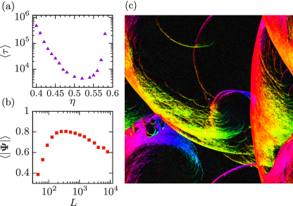
Figure 2: (a) Average inter-reversal time, $\langle\tau\rangle$ vs $\eta$ ($L=256$, $\sigma=35$). (b) Average global polarization vs system size with obstacle (red squares) and without (dashed line) ($\eta=0.5$, $\sigma=35$). (c) Snapshot of a $L=4096$ system ($\eta=0.5$, $\sigma=35$, colors as in Fig. 1(a)); at these parameters the system almost never recovers the homogeneous polar state. See related Movie S3 in SUP

Reversals due to the presence of an obstacle become exceedingly rare when decreasing $\eta$. To probe whether they can be triggered at low noise strengths, we study the fate of polar flocks in which we artificially introduce a dense blob of particles orientated against the main flow, and watch the subsequent evolution (details on our procedure can be found in SUP ). As for the fixed obstacle, we limit ourselves to circular blobs of diameter $\sigma_{\rm b}$ and density $\rho_{\rm b}$, and work with system sizes much larger than $\sigma_{\rm b}$ for which the number of particles in the blob remains much smaller than $N$. In the range of $\eta$ values where we can observe reversals triggered by an obstacle, a large-enough and dense-enough blob reverses the initial flow. These blob-induced reversals are similar to obstacle-induced ones, the main difference being that the blob vanishes completely after its introduction. As $\eta$ is decreased, though, a given blob does not always lead to a reversal (see Movie S4 in SUP ). We find that $P_{\rm rev}$, the probability to reverse the flow upon the introduction of a given blob, varies from 0 to 1 when $\eta$ is increased, in a manner consistent with a hyperbolic tangent (Fig. 3(a)). This allows to define a transitional value $\eta^{*}$ (at $P_{\rm rev}=\tfrac{1}{2}$), and to see how it varies with $\rho_{\rm b}$ and $\sigma_{\rm b}$. As expected, this procedure works not only for the $\eta$ values ‘accessible’ with a fixed obstacle, but also with smaller values. However, as shown in Fig. 3(b), we identify a minimal value $\eta\simeq 0.40$ below which no blob, however dense, triggers a reversal. This suggests that only a fraction of the Toner-Tu phase is destroyed by a single localized obstacle.

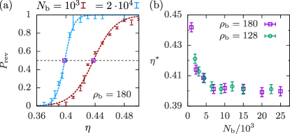
Figure 3: Reversals triggered by the introduction of a finite blob of counter-propagating particles ($L=1024$). (a) Reversal probability $P_{\rm rev}$ vs $\eta$ at different $N_{\rm b}$ for $\rho_{\rm b}=180$, magenta squares indicate the estimated value for $\eta^{*}$. (b) $\eta^{*}$ for different $\rho_{\rm b}$ as a function of the number of particles in the blob $N_{\rm b}$.

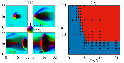
Figure 4: Simulations of the Boltzmann equation (3) truncated at $K=4$ at system density $\rho_{0}=2$ and blob radius $\sigma_{\rm b}=2$. (a) Snapshots showing the evolution of the momentum field ($f_{1}=p_{x}+ip_{y}$) at noise $\eta=0.5$ after introduction of a blob with density $\rho_{\rm b}=8\rho_{0}$ in the ordered solution at time $t=0$. Note that the bivariate color map leads dilute disordered regions to appear darker. (b) Fate of blob in the $(\rho_{\rm b},\eta)$ plane: dots mark parameters leading to a reversal, while squares indicate where no reversal occurs. More details about the numerical protocol in SUP .

We finally explore whether continuous kinetic or hydrodynamic theories of polar flocks can also account for the phenomena reported above. For numerical convenience, we did not consider a fixed obstacle but only studied the fate of an initial small circular blob oriented against the main order. Remarkably, when using standard hydrodynamic Toner-Tu equations SUP no blob, however dense, seems able to trigger a growing counter-propagating band (and thus a reversal) anywhere in the ordered phase. The initial blob splits into two wings which ‘diffuse away’ (not shown). On the other hand, reversals do occur when considering low-level truncations of the Boltzmann equation for the Vicsek/polar class. This equation has been introduced elsewhere and mostly used to derive hydrodynamic theories Bertin et al. (2006, 2009); Peshkov et al. (2014); Chaté and Mahault (2021). Here we only provide a sketch, with all details given in SUP . The Boltzmann equation governs the one-body probability distribution function $f({\bf r},\theta,t)$ of finding a particle with velocity orientation $\theta$ at position ${\bf r}$ and time $t$:

$$\partial_{t}f+v_{0}\,{\bf e}(\theta)\!\cdot\!\nabla f=I_{\rm sd}[f]+I_{\rm co}[f]$$ (2)

where ${\bf e}(\theta)$ is the unit vector along $\theta$, and $I_{\rm sd}$ and $I_{\rm co}$ are self-diffusion and collision integrals. Expanding $f$ in angular Fourier modes $f({\bf r},\theta,t)=\tfrac{1}{2\pi}\sum_{k}f_{k}({\bf r},t)\exp(-ik\theta)$, the Boltzmann equation is turned into a hierarchy of coupled partial differential equations for the complex fields $f_{k}$:

$$\partial_{t}f_{k}+\tfrac{1}{2}\left(\triangledown^{*}\!f_{k+1}\!+\!\triangledown f_{k-1}\right)=\alpha_{k}f_{k}+\sum_{q}J_{k,q}f_{q}f_{k-q}$$ (3)

where $\triangledown=\partial_{x}+i\partial_{y}$, and $\alpha_{k}$ and $J_{k,q}$ are coefficients depending on parameters given in SUP . The Toner-Tu hydrodynamic theory is recovered when truncating and closing (3) using a scaling ansatz which essentially sets all $f_{k>2}=0$, and enslaves $f_{2}$, the nematic order field, to the polar field $f_{1}$. Here, after realizing that this theory cannot account for reversals, we considered abrupt truncations of (3) at order $K$, simply setting $f_{k>K}=0$ and integrating the remaining set of $K+1$ equations (for numerical details, see SUP ).

The lowest order $K$ at which we could observe a full reversal is $K=4$ . Fig. 4(a) shows snapshots of the evolution of an initial blob in this case (see also Movie S5 in SUP ), which is remarkably similar to that observed with the Vicsek model. That our set of equations is able to reproduce the development of a reversal is testimony that this dynamics is essentially deterministic. This allows us to scan parameter space systematically using single runs. In Fig. 4(b) we show the result of such an exploration in the $(\eta,\rho_{\rm b})$ plane. We find an abrupt limit in $\eta$ below which no blob can lead to a reversal (see Movie S6 in SUP ), again in agreement with the microscopic-level results shown in Fig. 3(b).

To summarize, we have shown that arbitrarily large polar flocks are susceptible to the presence of a single small obstacle: In a fairly wide region of the ordered Toner-Tu phase, the obstacle triggers counter-propagating dense bands leading to reversals of the flow. We observed reversals at the microscopic level using two distinct rules for particle-obstacle collisions, and also in truncations of the relevant Boltzmann equation. This stresses the genericity of reversals. However, we were unable to observe them within the standard Toner-Tu hydrodynamic theory. This may be a manifestation of the limitations of simple hydrodynamic theories to account for highly nonlinear spatiotemporal dynamics (see Cai et al. (2019) for a similar observation in the context of active nematics).

In very large systems we observe complex chaotic dynamics where the bands triggered initially interact among themselves and with the obstacle. Increasing system size, the homogeneous Toner-Tu fluid is never recovered. Extrapolating to the infinite-size limit, the global order is thus broken. As a matter of fact, one can wonder whether the complicated band chaos observed could be sustained even in the absence of the obstacle. This important question, the answer to which looks so far only accessible via the observation of extremely large systems, is left for future studies.