Comprehensive study of muon-catalyzed nuclear reaction processes in the dt$\mu$ molecule

Abstract

Muon catalyzed fusion ($\mu$CF) has recently regained considerable research interest owing to several new developments and applications. In this regard, we have performed a comprehensive study of the most important fusion reaction, namely $(dt\mu)_{J=v=0}\to\alpha+n+\mu+17.6\,{\rm MeV}\>$ or $\;(\alpha\mu)_{nl}+n+17.6\,{\rm MeV}$. For the first time, the coupled-channels Schrödinger equation for the reaction is solved, satisfying the boundary condition for the muonic molecule $(dt\mu)_{J=v=0}$ as the initial state and the outgoing wave in the $\alpha n\mu$ channel. We employ the $dt\mu$- and $\alpha n\mu$-channel coupled three-body model. All the nuclear interactions, the $d$-$t$ and $\alpha$-$n$ potentials, and the $dt$-$\alpha n$ channel-coupling nonlocal tensor potential are chosen to reproduce the observed low-energy ($1-300$ keV) astrophysical $S$-factor of the reaction $d+t\to\alpha+n+17.6\,{\rm MeV}$, as well as the total cross section of the $\alpha+n$ reaction at the corresponding energies. The resultant $dt\mu$ fusion rate is $1.15\times 10^{12}\,{\rm s}^{-1}$. Substituting the obtained total wave function into the $T$-matrix based on the Lippmann-Schwinger equation, we have calculated absolute values of the fusion rates $\lambda_{\rm f}^{\rm bound}$ and $\lambda_{\rm f}^{\rm cont.}$ going to the bound and continuum states of the outgoing $\alpha$-$\mu$ pair, respectively. We then derived the initial $\alpha$-$\mu$ sticking probability $\omega_{S}^{0}=\lambda_{\rm f}^{\rm bound}/(\lambda_{\rm f}^{\rm bound}+\lambda_{\rm f}^{\rm cont.})=0.857\%$, which is $\sim\!7\%$ smaller than the literature values $(\simeq 0.91-0.93\%)$ , and can explain the recent observations (2001) at high D/T densities. We have much improved the sticking-probability calculation by employing the $D$-wave $\alpha$-$n$ outgoing channel with the non-local tensor-force $dt$-$\alpha n$ coupling and by deriving $\omega_{S}^{0}$ based on the absolute values of the $\lambda_{\rm f}^{\rm bound}$ and $\lambda_{\rm f}^{\rm cont.}$. We also calculate the absolute values for the momentum and energy spectra of the muon emitted during the fusion process. The most important result is that the peak energy is 1.1 keV although the mean energy is 9.5 keV owing to the long higher-energy tail. This is an essential result for the ongoing experimental project to realize the generation of an ultra-slow negative muon beam by utilizing the $\mu$CF for various applications e.g., a scanning negative muon microscope and an injection source for the muon collider.

I INTRODUCTION

In the mixture of deuterium (D) and tritium (T), an injected negatively charged muon ($\mu$) forms a muonic molecule with a deuteron ($d$) and a triton ($t$), namely, $dt\mu$. Since the mass of a muon is 207 times heavier than that of an electron, the nuclear wave funcitons of $d$ and $t$ overlap inside the $dt\mu$ molecule, which instantly results in an intramolecular nuclear fusion reaction $d+t\to$ $\alpha+n+17.6\,{\rm MeV}$. After this reaction, the muon becomes free and can facilitate another fusion reaction (Fig. 1). This cyclic reaction is called muon catalyzed fusion ($\mu$CF). Among various isotopic species of muonic molecules ($pp\mu$, $pd\mu$, $dd\mu$, $dt\mu$ and $tt\mu$), the $dt\mu$ has attracted particular attention in $\mu$CF with the expectation that it may be exploited as a future energy source.

The $\mu$CF has been dedicatedly studied since 1947 Frank (1947); Sakharov1948 , and is reviewed in Refs. Breunlich89 ; Ponomarev90 ; Froelich92 ; Nagamine98 . Efficiency of the $\mu$CF has been discussed in the literature as following: As seen in Fig. 1, the muon emitted after the $d$-$t$ fusion sticks to the $\alpha$ particle with a probability, $\omega_{S}^{0}$, and is lost from the cycle due to spending its lifetime ($\tau_{\mu}=2.2\times 10^{-6}$s) as a coupled entity, although the muon is reactivated (stripped) with a probability $R$ during the collision of an $(\alpha\mu)^{+}$ ion with the D-T mixture. The net loss-probability $\omega_{S}^{\rm eff}=\omega_{S}^{0}(1-R)$ is called effective sticking probability, whereas $\omega_{S}^{0}$ is referred to as initial sticking probability. The number of fusion events, $Y_{\mathrm{f}}$, catalyzed by one muon is essentially represented as Ponomarev90

$$Y_{\mathrm{f}}\simeq\left(\omega_{S}^{\rm eff}+\lambda_{0}/\lambda_{c}\phi\right)^{-1}$$ (1)

where $\lambda_{0}=1/\tau_{\mu}=0.455\times 10^{6}$ s^-1, $\lambda_{c}$ is a cycle rate, and $\phi$ is a target density relative to the liquid hydrogen ($4.25\times 10^{22}$ atoms cm^-3). A typical parameter set of $\omega_{S}^{\rm eff}\sim 0.5\%$ Ishida2001 and $\lambda_{c}\sim 1.1\times 10^{8}$ s^-1 Kawamura2003 at $\phi=1.25$ results in $Y_{\mathrm{f}}\sim 120$, which produces $\sim\!2.1$ GeV per a muon. A literature reported $Y_{\mathrm{f}}\sim 150$ Jones1986nature which was the highest value known so far, and results in $\sim\!2.6$ GeV, whereas $\sim\!5$ GeV of energy is required to generate a muon in accelerator; the efficiency of $\mu$CF for energy production is approximately half that required to achieve a scientific break-even. If $\omega_{S}^{\rm eff}$ is omitted in Eq. (1), $Y_{\mathrm{f}}\sim\!300$ cycles is obtained. On the other hand, if we omit $\lambda_{0}/\lambda_{c}\phi$ from Eq. (1), we have $Y_{\mathrm{f}}\sim\!200$. Therefore, the low efficiency of the $\mu$CF comes from both parameters of $\omega_{S}^{\rm eff}$ and $\lambda_{c}$; it is desirable to examine $\omega_{S}^{0}$, $R$ and $\lambda_{c}$ carefully.

Although the fusion yield $Y_{\mathrm{f}}$ as well as the fundamental parameters $\omega_{S}^{0}$, $R$ and $\lambda_{c}$ have been often investigated in liquid/solid targets thus far, such a cold target $\mu$CF would not be realistic as a practical energy source due to the low thermal efficiency of the Carnot cycle. The experimental knowledge of $\mu$CF at high-temperature conditions, however, is limited.

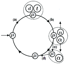
Figure 1: Schematic diagram of the $\mu$CF cycle by a muon injected into the D-T mixture. (a) Formation of $dt\mu$ molecule, (b) fusion reaction, (c) $\alpha$-$\mu$ initial sticking, and (d) muon reactivation.

The $\mu$CF has recently regained considerable interest owing to several new developments and applications. They are grouped into the following two types:

• To realize the production of energy by the $\mu$CF using the high-temperature gas target of the D-T mixture with high thermal efficiency.

• To realize an ultra-slow negative muon beam by utilizing the $\mu$CF for various applications e.g., a scanning negative muon microscope and an injection source for the muon collider.

They are explained as follows:

Type I): The $\mu$CF kinetics model in high-temperature gas targets is re-examined, including the excited (resonant) muonic molecules and fusion in-flight processes Iiyoshi et al. (2019); Yamashita et al. (submitted). Recent improvements in the energy resolution of X-ray detectors facilitate the examination of the dynamics of muon atomic processes Okada et al. (2020); Paul et al. (2021); Okumura et al. (2021), and may allow for the detection of the resonance states of muonic molecules during the $\mu$CF cycle. An intense muon beam Miyake et al. (2014) also creates the upgraded conditions required to explore these $\mu$CF fundamental studies. In parallel to the re-examination of the $\mu$CF kinetics model, there is a new proposal to strongly reduce the $\alpha$-$\mu$ sticking probability by boosting the negative muon stripping using resonance radio-frequency acceleration of $(\alpha\mu)^{+}$ ions in a spatially located D-T mixture gas stream Mori2021 . In addition to studies on the $\mu$CF as possible energy sources, the 14.1 MeV neutron has been considered as a source for the mitigation of long-lived fission products (LLFPs) with nuclear transmutation Yamamoto2021 . Since the mitigation of LLFPs requires a well-defined condition for a neutron beam, $\mu$CF-based monochromatic neutrons would be more suitable than those from a nuclear reactor and/or spallation neutron sources.

Type II): In general, muon beams generated by accelerators have $\sim$ MeV kinetic energies. At present, the negative muon beam, with a size of a few tens of millimeters, has proven to be suitable for non-destructive elemental analysis Rosen (1971); Daniel (1984); Kubo (2016) in various research fields such as archeology, earth-and-planetary science, and industry. In contrast to the accelerator-based muon beam, the mean kinetic energy of the muon released after the $\mu$CF reaction is $\sim\!10$ keV since the $dt\mu$ molecule nearly takes the $(^{5}{\rm He}\mu)_{1s}$ configuration at the instant of the fusion reaction. Therefore, the $\mu$CF can be utilized as a means for beam cooling  Nagamine (1989); NagamineMCF199091 ; Nagamine1996Hyp103 ; Strasser et al. (1993); Strasser1996 . Recently, the aim has been to produce a negative muon beam by reducing the beam size to an order of 10 $\mu$m using a set of beam optics, by utilizing the muons emitted by the $\mu$CF. This beam is called an ultra-slow negative muon beam Nagamine (1989); Nagamine1996Hyp103 ; Natori2020 , which will facilitate various applications such as a scanning negative muon microscope, as well as an injection source for a muon collider Nagamine1996Hyp103 . The scanning negative muon microscope that can utilize characteristic muonic X-rays will allow for three-dimensional analysis of elements and isotopes. Owing to the high penetrability of muon, such a microscope can be applied to biological samples under the atmospheric environment. Experiments for direct observation of the muon released after the $\mu$CF using a layered hydrogen thin disk target are in progress Nagamine (1989); NagamineMCF199091 ; Strasser et al. (1993); Nagamine1996Hyp103 ; Strasser1996 ; Okutsu et al. (2021); Yamashita et al. (2021).

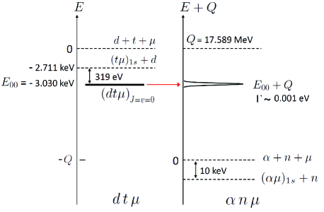
Figure 2: Schematic illustration of the energy relation between the $dt\mu$ and $\alpha n\mu$ channels. Owing to the nuclear interaction, the muonic molecular bound state $(dt\mu)_{J=v=0}$ at $E_{00}=-3.030$ keV becomes an extremely narrow Feshbach resonance that decays into the $\alpha+n+\mu$ and $(\alpha\mu)_{nl}+n$ continuum states. The width of the resonance ($\Gamma\sim 10^{-3}$ eV) was already derived, for example, using the $d$-$t$ optical-potential-model calculation of the reaction (3) Kamimura89 ; Bogdanova ; Bogdanova89 and by the $R$-matrix method Struensee88a ; Szalewicz90 ; Hale93 ; Hu1994 ; Cohen1996 ; Jeziorski91 .

Here, we note that two of the present authors (Y.K. and T.Y.) have contributed to the aforementioned studies of Type I in Refs. Iiyoshi et al. (2019); Yamashita et al. (submitted) and Type II in Refs. Okutsu et al. (2021); Yamashita et al. (2021).

The purpose of the present paper is that considering the latest developments regarding the new $\mu$CF applications, we thoroughly investigate the mechanism of the nuclear reaction

$$(dt\mu)_{J=v=0} \to\;\alpha\,+n\,+\mu+17.6\,\mbox{MeV}$$ (2a)

$$\searrow\;(\alpha\mu)_{nl}+n+17.6\,\mbox{MeV},$$ (2b)

by employing a sophisticated framework that has not been explored in the literature work on this reaction.

The reaction (2) is the most important among the nuclear reactions in $\mu$CF, but it has a complicated mechanism. Figure 2 illustrates schematically the energy relation between the $dt\mu$ and $\alpha n\mu$ channels; the molecular bound state $(dt\mu)_{J=v=0}$ becomes an extremely narrow Feshbach resonance with $\Gamma\!\sim\!10^{-3}$ eV Kamimura89 ; Bogdanova ; Bogdanova89 ; Struensee88a ; Szalewicz90 ; Hale93 ; Hu1994 ; Cohen1996 ; Jeziorski91 that decays into the $\alpha+n+\mu\,$ and $\,(\alpha\mu)_{nl}+n$ continuum states, owing to the nuclear interactions.

Therefore, due to the difficulty of the problem, the reaction (2) has not been studied in the literature using sufficiently sophisticated methods. Another reason is that such a precise calculation of the reaction has not been required in previous $\mu$CF studies; the required quantities were the fusion rate $\lambda_{\rm f}(=\Gamma/\hbar)$ and the $\alpha$-$\mu$ initial sticking probability $\omega_{S}^{0}$, which were calculated using approximate models (cf. Secs. 7 and 8 of the $\mu$CF review paper Froelich92 ), for example, in Ref. Kamimura89 by one of the present authors (M.K.).

For the new situation of $\mu$CF mentioned in Types I and II, it is desirable to precisely calculate the following quantities of the reaction (2):

• Reaction rates, in absolute values, going to the individual bound and continuum states of the outgoing $\alpha$-$\mu$ pair, together with the $\alpha$-$\mu$ sticking probability $\omega_{S}^{0}$ based on those reaction rates.

• Momentum and energy spectra, in absolute values, of the muon emitted by the fusion reaction.

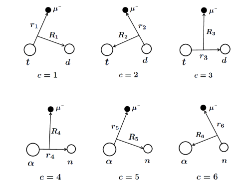
Figure 3: All the sets of Jacobi coordinates in the $dt\mu$ system $(c=1,2$ and 3) and in the $\alpha n\mu$ system $(c=4,5$ and 6).

To calculate these quantities and conduct additional analyses, we employ the $dt\mu$- and $\alpha n\mu$-channel coupled three-body model and perform the following:

• We first determine all the nuclear interactions (the $d$-$t$ and $\alpha$-$n$ potentials and the $dt$-$\alpha n$ channel coupling potential) to reproduce the observed astrophysical $S$-factor of the reaction

  $$d+t\to\alpha+n+17.6\>\mbox{MeV}$$ (3)

  at the low-energies of $1-300$ keV Sfactor-exp as well as the total cross section of the $\alpha+n$ reaction at the corresponding energies Haesner (see Sec. II).

• We solve a coupled-channels three-body Schrödinger equation on the Jacobi coordinates in Fig. 3, satisfying the boundary condition to have the muonic molecular bound state $(dt\mu)_{J=v=0}$ as the initial state (as the source term of Schrödinger equation) and the outgoing wave in the $\alpha n\mu$ channel with the 17.6-MeV $D$-state $\alpha$-$n$ relative motion based on the observation (see Sec. III).

• We calculate the quantities a) and b) by substituting the obtained total wave function into the $T$-matrix elements for a) and b) based on the Lippmann-Schwinger equation Lippmann (see Secs. IV,V and VI).

The reliability of these calculations shall be carefully examined as follows: The fusion rate $\lambda_{\rm f}$ (the number of fusions per second) is calculated in the three different prescriptions:

• $\lambda_{\rm f}$ from the $S$-matrix of the asymptotic amplitude of the total wave function solved using the coupled-channels Schrödinger equation (see Sec. III).

• $\lambda_{\rm f}$ from the $T$-matrix calculation of the reaction rates mentioned in item a) (see Sec.V).

• $\lambda_{\rm f}$ from the $T$-matrix calculation of the muon spectra mentioned in item b) (see Sec. VI).

If our total wave function is the exact rigorous solution of the coupled-channels Schrödinger equation, the fusion rates $\lambda_{\rm f}$ obtained by A)-C) should be equal according to the Lippmann-Schwinger equation that is equivalent to the Schrödinger equation. However, since the function space employed in our total wave function is not complete, the resultant $\lambda_{\rm f}$ are not equal, but they should be consistent with each other. This check of $\lambda_{\rm f}$ is one of the highlights of the present paper.

The authors possess their own three methods to solve the present coupled-channels three-body Schrödinger equation. Namely, the Kohn-type variational method for the reactions between composite particles Kamimura77 , the Gaussian expansion method (GEM) for few-body systems Kamimura88 ; Kameyama89 ; Hiyama03 here for describing the $(dt\mu)$ molecule nonadiabatically Kamimura88 , and the continuum-discretized coupled-channels (CDCC) method Kamimura86 ; Austern ; Yahiro12 here for discretizing the $\alpha$-$\mu$ and $\alpha$-$n$ continuum states.

This paper is organized as follows. In Sec. II we will determine all the nuclear interactions used in this work to reproduce the observed $S$-factor of the reaction (3) and the total cross section of the $\alpha+n$ reaction. In Sec. III we solve the coupled-channels Schrödinger equation for the reaction (2). Section IV is devoted to providing an overview of the $T$-matrix framework based on the Lippmann-Schwinger equation. In Sec. V, based on the $T$-matrix calculation, we derive the reaction rates going to the $\alpha$-$\mu$ bound and continuum states. In Sec. VI, we also derive the momentum and energy spectra of the muon ejected from the fusion reaction. Finally, a summary is given in Sec. VII.

II Nuclear interactions for low-energy $d+t\to\alpha+n$ reaction

To investigate the mechanism of the $\mu$CF reaction (2) based on the $dt\mu$- and $\alpha n\mu$-channels coupled three-body model, it is necessary to use the nuclear interactions (the $d$-$t$ and $\alpha$-$n$ potentials and the $dt$-$\alpha n$ coupling potential) that reproduce the observed low-energy astrophysical $S$ factor of the reaction (3) (cf. Fig. 4) as well as the total cross section of the $\alpha+n$ reaction at the corresponding energies (cf. Fig. 5).

Considering that a similar framework for channel coupling will also be used in the study of $\mu$CF reaction (2), we apply the same coordinates ${\bf r}_{3}$ and ${\bf r}_{4}$ in Fig. 3 to the $d$-$t$ and $\alpha$-$n$ relative coordinates, respectively, in this section.

The total wave function of the system has spin-parity $I=\frac{3}{2}^{+}$ in the energy region of the resonance and below. It is known that the $d$-$t$ channel has $S$-wave and spin $\frac{3}{2}$ and the $\alpha$-$n$ channel has $D$-wave with spin $\frac{1}{2}$ coupled to $I=\frac{3}{2}^{+}$. Let $E$ denote the c.m. energy of the $d$-$t$ relative motion. The total wave function is written as

$$\!\!\!\!\!\!\Phi_{\frac{3}{2}M}(E) = \phi_{0}({\bf r}_{3})\,\chi_{\frac{3}{2}M}(dt)+\big{[}\psi_{2}({\bf r}_{4})\,\chi_{\frac{1}{2}}(\alpha n)\big{]}_{\frac{3}{2}M}$$ (4)

$$= \frac{\bar{\phi}_{0}(r_{3})}{r_{3}}\,Y_{00}(\widehat{{\bf r}}_{3})\,\chi_{\frac{3}{2}M}(dt)$$

$$+ \frac{\bar{\psi}_{2}(r_{4})}{r_{4}}\,\big{[}Y_{2}(\widehat{{\bf r}}_{4})\,\chi_{\frac{1}{2}}(\alpha n)\big{]}_{\frac{3}{2}M}\>,$$

which has the asymptotic behavior

$$\bar{\phi}_{0}(r_{3})\stackrel{{\scriptstyle r_{3}\to\infty}}{{\longrightarrow}}\!\!\!U_{0}^{(-)}(k_{3},r_{3})-S_{0}^{(dt)}\,U_{0}^{(+)}(k_{3},r_{3}),\;\;$$ (5)

$$\bar{\psi}_{2}(r_{4})\stackrel{{\scriptstyle r_{4}\to\infty}}{{\longrightarrow}}\quad\quad-\,\sqrt{\frac{v_{3}}{v_{4}}}\,S_{2}^{(dt,\alpha n)}\,U_{2}^{(+)}(k_{4},r_{4}),\;\;$$ (6)

$$U_{L}^{(\pm)}(k,r)=G_{L}(k,r)\mp iF_{L}(k,r),$$ (7)

where $k_{3}(k_{4})$ and $v_{3}(v_{4})$ are the wave number and the velocity of relative motion along ${\bf r}_{3}({\bf r}_{4})$, respectively, and $F_{L}$ and $G_{L}$ are the regular and irregular Coulomb functions, respectively.

We assume that the $S$- and $D$-state wave functions are coupled to each other by the following tensor force, which is nonlocal between ${\bf r}_{3}$ and ${\bf r}_{4}$;

$$\!\!\!\!\!\!\!\!\!V_{dt,\alpha n}^{({\rm T})}({\bf r}_{3},{\bf r}_{4}) \!\!\!=\!\!\! v^{({\rm T})}(r_{34},R_{34})\big{[}Y_{2}({\widehat{\bf r}}_{34})\,{\cal S}_{2}(dt,\alpha n)\big{]}_{00},$$ (8)

$$\!\!\!\!\!\!\!\!\!v^{({\rm T})}(r_{34},R_{34}) \!\!=\!\! v_{0}^{({\rm T})}r_{34}^{2}\,e^{-\mu\,r_{34}^{2}-\mu^{\prime}R_{34}^{2}},$$ (9)

where ${\bf r}_{34}={\bf r}_{3}-{\bf r_{4}}$ and ${\bf R}_{34}={\bf r}_{3}+{\bf r_{4}}$. In Eq. (8), ${\cal S}_{2}(dt,\alpha n)$ is a spin-tensor operator composed of spins of $dt$- and $\alpha n$-pairs. However, it is not necessary to know the explicit form of ${\cal S}_{2}(dt,\alpha n)$ in the present work, as will be explained in the paragraph below Eq. (15).

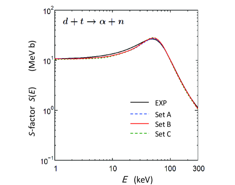
Figure 4: Calculated and observed $S$-factor $S(E)$ of the $d+t\to\alpha+n$ reaction with respect to the c.m. energy $E$ of the incoming $d$-$t$ wave. The three curves for Sets A, B, and C are obtained using the nuclear interactions listed in Table I. The black curve (EXP) is taken from a review paper Sfactor-exp ; it fits the literature data using the function $S(E)=(26-0.361E+248E^{2})/(1+((E-0.0479)/0.0392)^{2}){\rm MeV}\,{\rm b}$ ($E$ in MeV). The calculated curves lie within the error range of the data.

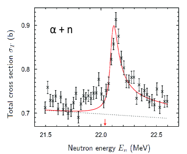
Figure 5: The total cross section $\sigma_{T}(E_{n})$ of the $\alpha+n$ reaction based on the observation Haesner and the present calculation with the nuclear interactions Set B (the red curve), where $E_{n}$ is the neutron incident energy. The dotted line denotes the background cross section based on partial waves other than the $D_{3/2^{+}}$ wave Haesner ; Barker . The calculated red curve for the $I={\frac{3}{2}}^{+}$ state is piled on the background dotted line. The peak at $E_{n}\approx 22.1$MeV corresponds to the peak in Fig. 4 for the $d$-$t$ channel. The $d$-$t$ threshold $(E=0)$ corresponds to $E_{n}=22.03$ MeV (at the red arrow) in the $\alpha$-$n$ channel.

The coupled-channels Schrödinger equation required to solve $\phi_{0}({\bf r}_{3})$ and $\psi_{2}({\bf r}_{4})$ is written as

$$\!\!\!\!(H_{dt}-E)\,\phi_{0}({\bf r}_{3})\,\chi_{\frac{3}{2}M}(dt)=-V^{({\rm T})}_{dt,\alpha n}\>\big{[}\psi_{2}({\bf r}_{4})\,\chi_{\frac{1}{2}}(\alpha n)\big{]}_{\frac{3}{2}M},\!\!\!$$ (10a)

$$\!\!\!\!\!\!\left(H_{\alpha n}-(E+Q)\right)\,\big{[}\psi_{2}({\bf r}_{4})\,\chi_{\frac{1}{2}}(\alpha n)\big{]}_{\frac{3}{2}M}\qquad\qquad\qquad\;\;\;$$

$$\!\!\!\!\!\!=-V^{({\rm T})}_{\alpha n,dt}\>\phi_{0}({\bf r}_{3})\,\chi_{\frac{3}{2}M}(dt),\quad$$ (10b)

where $Q=17.589$ MeV and

$$H_{dt} = T_{{\bf r}_{3}}+V_{dt}^{({\rm N})}(r_{3})+V_{dt}^{({\rm C})}(r_{3}),\;\;$$ (11)

$$H_{\alpha n} = T_{{\bf r}_{4}}+V_{\alpha n}^{({\rm N})}(r_{4}),$$ (12)

$$V^{({\rm T})}_{dt,\alpha n} = \int d{\bf r}_{4}\>V_{dt,\alpha n}^{({\rm T})}({\bf r}_{3},{\bf r}_{4}).$$ (13)

The coupled-channels Schrödinger equation (10) with the scattering boundary condition (5)-(7) can be accurately solved by using the couple-channels Kohn-type variational method for composite-particle reactions that was proposed by one of the authors (M.K.) Kamimura77 and has been employed in the literature in three-body transfer reactions, for example, in Refs. Kawai86 ; Kino93a ; Kamimura09 .

When the matrix element of the tensor force is calculated, the spin part $S^{({\rm T})}_{0}$ is factored out as follows:

$$\!\!\!\!\!\!\!\!\!\!\!\!\!\!\!\langle\,\big{[}\phi_{2}({\bf r}_{4})\,\chi_{\frac{1}{2}}(\alpha n)\big{]}_{\frac{3}{2}M}\,|\,V^{({\rm T})}_{\alpha n,dt}\,|\,\big{[}\phi_{0}({\bf r}_{3})\,\chi_{\frac{3}{2}}(dt)\big{]}_{\frac{3}{2}M}\rangle$$

$$\!\!\!\!\!\!\!\!\!\!\!\!\!\!\!\!=v^{({\rm T})}_{0}S^{({\rm T})}_{0}\langle\,\phi_{2m}({\bf r}_{4})|\,r_{34}^{2}\,e^{-\mu\,r_{34}^{2}-\mu^{\prime}R_{34}^{2}}|\,\big{[}Y_{2}({\widehat{\bf r}}_{34})\phi_{0}({\bf r}_{3})\big{]}_{2m}\rangle,\;$$ (14)

where

$$\!\!\!\!\!\!\!S^{({\rm T})}_{0}=\frac{1}{\sqrt{10}}\langle\,\chi_{\frac{1}{2}m_{s}}(\alpha n)\,|\,\big{[}{\cal S}_{2}(\alpha n,dt)\chi_{\frac{3}{2}}(dt)\big{]}_{\frac{1}{2}m_{s}}\rangle\>.$$ (15)

The R.H.S. of Eqs. (14) and (15) are independent of $m$ and $m_{s}$, respectively, and hence, the L.H.S. of Eqs. (14) does not depend on $M$. We shall verify, in Secs. III, V and VI, that the same $v^{({\rm T})}_{0}S^{({\rm T})}_{0}$ as above is factored out when calculating the three-body matrix elements of the tensor force and the $T$-matrix elements due to the same force. Consequently, we can treat the tensor force consistently throughout the present work without knowing the explicit forms of ${\cal S}_{2}(dt,\alpha n)$ and $S^{({\rm T})}_{0}$. It is sufficient to search for the optimum value of the product $v^{({\rm T})}_{0}S^{({\rm T})}_{0}$ when producing the observed data.

The nuclear $d$-$t$ potential and accompanied Coulomb potential are employed, respectively, in the form

$$\;V_{dt}^{{\rm(N})}(r_{3})=V_{0}/\{1+e^{(r_{3}-R_{0})/a}\},$$ (16)

$$V_{dt}^{({\rm C})}(r_{3})=\begin{cases}\frac{e^{2}}{R_{\rm c}}(\frac{3}{2}-\frac{r_{3}^{2}}{2R_{\rm c}^{2}})&\text{$(r_{3}<R_{\rm c}\!=\!R_{0})$},\\ \frac{e^{2}}{r_{3}}&\text{$(r_{3}\geq R_{\rm c}\!=\!R_{0})$}.\end{cases}$$ (17)

As the $\alpha$-$n$ potential $V_{\alpha n}^{({\rm N})}(r_{4})$, we employ the Kanada-Kaneko $\alpha$-$n$ potential Kaneko ; PTP-suppl-68-III (see Fig. 6), which is derived based on an equivalent local potential to the nonlocal kernel of the resonating-group method for the $\alpha$-$n$ system, and is often used in the $\alpha$-cluster-model calculations of light nuclei PTP-suppl-68-III . We then fix the potential as $V_{\alpha n}^{({\rm N})}(r_{4})$ throughout this work.

Table 1: Parameter Sets A, B, and C of the nuclear interactions $V_{dt}^{\rm(N)}(r_{3})$ in Eq. (16) and $V_{dt,\alpha n}^{\rm(T)}({\bf r}_{3},{\bf r}_{4})$ in Eq. (8) for reproducing the observed data in Figs. 4 and 5.

		$V_{0}$		$R_{0}$		$a_{0}$		$v_{0}^{({\rm T})}S_{0}^{({\rm T})}$		$\mu$		$\mu^{\prime}$
		(MeV)		(fm)		(fm)		$({\rm MeV}\,{\rm fm}^{-5})$		$({\rm fm}^{-2})$		$({\rm fm}^{-2})$
Set A		$-57.0$		$2.5$		$0.3$		$7.04$		$1/1.16^{2}$		$1/6.0^{2}$
Set B		$-37.2$		$3.0$		$0.5$		$5.43$		$1/1.16^{2}$		$1/6.0^{2}$
Set C		$-27.7$		$3.0$		$1.0$		$4.76$		$1/1.20^{2}$		$1/6.0^{2}$

As the nuclear interactions $V_{dt}^{({\rm N})}(r_{3})$ and $V^{({\rm T})}_{dt,\alpha n}({\bf r}_{3},{\bf r}_{4})$ introduced above are phenomenological ones, it is desirable to be shown that the calculated results for the reaction (2) are independent of the interaction details as long as they reproduce the observed data in Figs. 4 and 5. Concequently, three sets of the interactions, Sets A, B, and C shown in Table I, are examined. $V_{dt}^{\rm(N)}(r_{3})$ is acquired from the real part of the $d$-$t$ optical potentials A, B, and C in Ref. Kamimura89 with a slight change in $V_{0}$ while $R_{0}$ and $a_{0}$ are the same; in the study, the fusion rate $\lambda_{\rm f}=\mbox{(1.22 - 1.28)}\times 10^{12}{\rm s}^{-1}$ was derived using the optical-potential model. The potentials $V_{dt}^{({\rm N})}(r_{3})$ of Set B and $V_{\alpha n}^{({\rm N})}(r_{4})$ are illustrated in Fig. 6.

The reaction cross section $\sigma_{dt\to\alpha n}$ is given by

$$\sigma_{dt\to\alpha n}(E)=\frac{2I+1}{(2I_{d}+1)(2I_{t}+1)}\frac{\pi}{k_{3}^{2}}\,|S_{2}^{(dt,\alpha n)}|^{2},$$ (18)

and the $S$-factor $S(E)$ is derived from

$$\sigma_{dt\to\alpha n}(E)=S(E)\,e^{-2\pi\eta(E)}/E,$$ (19)

where $\eta(E)$ is the Sommerfeld parameter.

Calculated $S$-factor $S(E)$ using the nuclear interactions of Sets A, B, and C is illustrated in Fig. 4. The black curve represents the observed data summarized in a review paper  Sfactor-exp . All the calculated curves well reproduce the observed data within the error range of the data that are not shown here.

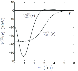
Figure 6: The nuclear $d$-$t$ potential $V_{dt}^{({\rm N})}(r)$ of Set B (the dashed curve) and the Kanada-Kaneko $\alpha$-$n$ potential $V_{\alpha n}^{({\rm N})}(r)$ Kaneko ; PTP-suppl-68-III for the even-parity case (the solid curve).

We then discuss the observed total cross section $\sigma_{T}(E_{n})$ of the $\alpha+n$ reaction for the $I={\frac{3}{2}}^{+}$ state Haesner given in Fig. 5. The nuclear interactions of Set B is used. The data should be explained by our calculation simultaneously as the $S$-factor $S(E)$ of the $d+t\to\alpha+n$ reaction. The total cross section can be expressed using our model as the sum of elastic and reaction cross sections, with the spin factor $\frac{2I+1}{(2I_{\alpha}+1)(2I_{n}+1)}=2$,

$$\!\!\!\!\!\!\sigma_{T}(E_{n})=\sigma_{\rm el.}(E_{n})+\sigma_{\rm re.}(E_{n})=\frac{4\pi}{k_{4}^{2}}\,[1-{\rm Re}(S_{2}^{(\alpha n)})],$$ (20)

with

$$\!\!\!\!\!\sigma_{\rm el.}(E_{n})=\frac{2\pi}{k_{4}^{2}}|1-S_{2}^{(\alpha n)}|^{2},\;\;\;\sigma_{\rm re.}(E_{n})=\frac{2\pi}{k_{4}^{2}}|S_{2}^{(\alpha n,dt)}|^{2},$$ (21)

and the unitarity $|S_{2}^{(\alpha n)}|^{2}+|S_{2}^{(\alpha n,dt)}|^{2}=1.$ The $S$-matrix elements are determined by the the asymptotic behavior, similarly to Eqs. (5) and (7),

$$\!\!\!\bar{\phi}_{0}(r_{3})\stackrel{{\scriptstyle r_{3}\to\infty}}{{\longrightarrow}} \!\!\quad\;\,\;\,-\,\sqrt{\frac{v_{4}}{v_{3}}}\,S_{2}^{(\alpha n,dt)}\,U_{0}^{(+)}(k_{3},r_{3}),\;\;$$ (22)

$$\!\!\!\bar{\psi}_{2}(r_{4})\stackrel{{\scriptstyle r_{4}\to\infty}}{{\longrightarrow}} \!\!\!\!\!U_{2}^{(-)}(k_{4},r_{4})-S_{2}^{(\alpha n)}\,U_{2}^{(+)}(k_{4},r_{4}).\;\;$$ (23)

Recall that when tuning the potential parameters to reproduce the $S$-factor $S(E)$ in Fig. 4, we fixed the $\alpha$-$n$ potential $V_{\alpha n}^{({\rm N})}(r_{4})$ and did not include the observed $\alpha+n$ data for fitting. Therefore, it is impressive to see in Fig. 5 that our result (the red curve) agrees well with the data.

However, this is not unexpected because of the following reason: The reaction $d+t\to\alpha+n$ in Fig. 4 is known as one of the most strongly channel-coupled reactions in nuclear physics Hale1987PRL ; Bogdanova1991 . Actually, at the peak, our calculation shows $|S_{2}^{(dt,\alpha n)}|\approx 1$ and $S_{0}^{(dt)}\approx 0$. Accordingly, we see that at the peak of the $\alpha+n$ reaction, $|S_{2}^{(\alpha n,dt)}|=|S_{2}^{(dt,\alpha n)}|\approx 1$ and $S_{2}^{(\alpha n)}\approx 0$ and hence $\sigma_{T}(I=\frac{3}{2}^{+})\approx 4\pi/k_{4}^{2}=0.19$ b with $k_{4}=0.824\,{\rm fm}^{-1}$. This is the peak value of $\sigma_{T}(I=\frac{3}{2}^{+})$ of the calculation (observation) in Fig. 5 piled on the dotted background line. It is asserted that even if we employ another $\alpha$-$n$ potential instead of the above $V_{\alpha n}^{({\rm N})}(r_{4})$, the same situation will be repeated as long as the observed data of the $d+t\to\alpha+n$ reaction are reproduced using the replaced $\alpha$-$n$ potential.

III Coupled-channels Schrödinger equation for $dt\mu$ fusion reaction

In this section, we formulate and solve the Schrödinger equation for the fusion reaction (2) using the nuclear interactions that were determined in the previous section and satisfying the boundary condition to have the muonic molecule $(dt\mu)_{J=v=0}$ as the initial state and the outgoing wave in the $\alpha n\mu$ channel. We first divide the fusion decay process into the following two steps:

Step 1)

Construction of the nonadiabatic wave function, denoted as $\mathring{\Phi}_{0}^{({\rm C})}({{\bf r}_{3},{\bf R}_{3}})$ (cf. Eq. (38)), of the initial $(dt\mu)_{J=v=0}$ state using the Coulomb potentials only Kamimura88 . The eigenenergy of the state, $E_{00}$, is given by

$$E_{00}=-0.003030\,{\rm MeV}$$ (24)

with respect to the $d+t+\mu$ threshold (cf. Fig. 2).

Step 2)

Decay of the $(dt\mu)_{J=v=0}$ state (now, a Feshbach resonance after the nuclear interactions are switched on) into the outgoing wave due to the nuclear $d$-$t$, $\alpha$-$n$ and $dt$-$\alpha n$ interactions. The kinetic energy of the outgoing wave with the wave number $k_{4}$ is given by

$$\frac{\hbar^{2}}{2\mu_{{\bf r}_{4}}}k_{4}^{2}=E_{00}+Q,\quad Q=17.589\,{\rm MeV}\,.$$ (25)

By employing the Step-1 wave function $\mathring{\Phi}_{0}^{({\rm C})}({{\bf r}_{3},{\bf R}_{3}})$ as the fixed source term of the coupled-channels Schrödinger equation, it becomes possible to impose the outgoing-wave boundary condition upon the $\alpha n\mu$ channel with no incoming wave for the entire system. The symbol ($\,\mathring{\>}\,$) placed on the top of $\mathring{\Phi}_{0}^{({\rm C})}({{\bf r}_{3},{\bf R}_{3}})$ is to show ’given’ before solving the Schrödinger equation of Step 2. $\mathring{\Phi}_{0}^{({\rm C})}({{\bf r}_{3},{\bf R}_{3}})$ will be calculated in Sec. III A.

The total angular momentum of the entire system is $\frac{3}{2}$ with its $z$-component $M$ similarly to the $dt$-$\alpha n$ case in Sec. II B (muon spin is neglected). We then describe the total wave function in term of the three parts based on the aforementioned two steps as follows:

$$\Psi_{\frac{3}{2}M}^{(+)}(E)=\mathring{\Psi}_{\frac{3}{2}M}^{({\rm C})}(dt\mu)+\Psi_{\frac{3}{2}M}^{({\rm N})}(dt\mu)+\Psi_{\frac{3}{2}M}^{(+)}(\alpha n\mu),$$ (26)

with

$$\mathring{\Psi}_{\frac{3}{2}M}^{({\rm C})}(dt\mu)=\mathring{\Phi}_{0}^{({\rm C})}({{\bf r}_{3},{\bf R}_{3}})\,\chi_{\frac{3}{2}M}(dt),$$ (27)

$$\Psi_{\frac{3}{2}M}^{({\rm N})}(dt\mu)=\Phi_{0}^{({\rm N})}({{\bf r}_{3},{\bf R}_{3}})\,\chi_{\frac{3}{2}M}(dt),$$ (28)

$$\Psi_{\frac{3}{2}M}^{(+)}(\alpha n\mu)=\big{[}\Phi_{2}^{(+)}({{\bf r}_{4},{\bf R}_{4}})\,\chi_{\frac{1}{2}}(\alpha n)\big{]}_{\frac{3}{2}M}\,.$$ (29)

Here, $\mathring{\Phi}_{0}^{({\rm C})},\Phi_{0}^{({\rm N})}$ and $\Phi_{2}^{(+)}$ are spatially $S\!$-, $S\!$- and $D$-wave functions, respectively. The spin functions $\chi_{\frac{3}{2}M}(dt)$ and $\chi_{\frac{1}{2}M}(\alpha n)$ were introduced in Eq. (4). However, the explicit form of the spin functions is not necessary because the phenomenological spin-tensor operator ${\cal S}_{2}(dt,\alpha n)$ and its matrix element $S_{0}^{(T)}$ of Eq. (15) are used.

In Eq. (26), the first component $\mathring{\Psi}_{\frac{3}{2}M}^{({\rm C})}(dt\mu)$ becomes the fixed source term of the coupled-channels Schrödinger equation. The second component $\Psi_{\frac{3}{2}M}^{({\rm N})}(dt\mu)$ is introduced to describe the $d$-$t$ relative motion due to the nuclear interactions. The third term $\Psi_{\frac{3}{2}M}^{(+)}(\alpha n\mu)$ is for the outgoing $\alpha n\mu$ channel. We can then derive the fusion rate from the asymptotic behavior of $\Psi_{\frac{3}{2}M}^{(+)}(\alpha n\mu)$.

The coupled-channels Schrödinger equation required to solve $\Psi_{\frac{3}{2}M}^{({\rm N})}(dt\mu)$ and $\Psi_{\frac{3}{2}M}^{(+)}(\alpha n\mu)$ can be written as

$$\!\!\!\!\!\!\!\!\!\!\!\!\big{(}H_{dt\mu}-E_{00}\big{)}\left[\mathring{\Psi}_{\frac{3}{2}M}^{({\rm C})}(dt\mu)+\Psi_{\frac{3}{2}M}^{({\rm N})}(dt\mu)\right]\qquad$$

$$\qquad\quad=-V^{({\rm T})}_{dt,\alpha n}\>\Psi_{\frac{3}{2}M}^{(+)}(\alpha n\mu),$$ (30a)

$$\big{(}H_{\alpha n\mu}-(E_{00}+Q)\big{)}\,\Psi_{\frac{3}{2}M}^{(+)}(\alpha n\mu)\qquad\qquad\;\;$$

$$\quad\quad\qquad\qquad=-V^{({\rm T})}_{\alpha n,dt}\>\left[\mathring{\Psi}_{\frac{3}{2}M}^{({\rm C})}(dt\mu)+\Psi_{\frac{3}{2}M}^{({\rm N})}(dt\mu)\right],\!\!\!\!\!\!\!\!$$ (30b)

where

$$\!\!\!\!H_{dt\mu} = T_{{\bf r}_{c}}+T_{{\bf R}_{c}}+V_{t\mu}^{({\rm C})}(r_{1})+V_{d\mu}^{({\rm C})}(r_{2})$$ (31)

$$+ V_{dt}^{({\rm C})}(r_{3})+V_{dt}^{({\rm N})}(r_{3}),\;\;(c=1,2\>\mbox{or}\>3),$$

$$\!\!\!\!H_{\alpha n\mu} = T_{{\bf r}_{4}}+T_{{\bf R}_{4}}+V_{\alpha n}^{({\rm N})}(r_{4})+V_{\alpha\mu}^{({\rm C})}(r_{5}),$$ (32)

$$\!\!\!\!V^{({\rm T})}_{dt,\alpha n} = \int d{\bf r}_{4}V_{dt,\alpha n}^{({\rm T})}({\bf r}_{3},{\bf r}_{4}).$$ (33)

An outline of the manner in which the three-body coupled-channels Schrödinger equation (30) is solved is provided based on the following senario presented in i) to iv):

i) It is to be noted that the kinetic energy (17.6 MeV) of the $\alpha$-$n$ relative motion is much larger than the potential energy (in the order of 10 keV) of $V_{\alpha\mu}^{({\rm C})}(r_{5})$, which can be neglected; the muon is located nearly around the $({\rm He}\mu)_{1s}$ orbital with the Bohr radius $\sim\!$ 130 fm when the fusion takes place in the $dt\mu$ molecule. Therefore, when solving the Schrödinger equation (30), the Coulomb potential $V_{\alpha\mu}^{({\rm C})}(r_{5})$ is omitted from $H_{\alpha n\mu}$ (32) for the $\alpha n\mu$ channel. The contribution of the potential $V_{\alpha\mu}^{({\rm C})}(r_{5})$ to the fusion rate $\lambda_{\rm f}$ is afterwards estimated by calculating the related $T$-matrix elements, which is then added to $\lambda_{\rm f}$ as a correction. A similar methodology can be followed for the contribution to the energy and momentum spectra of the emitted muons. Those contributions are found to be small (cf. Sec. VI).

ii) First, Eq. (3.7a) is solved with switching off the coupling to the $\alpha n\mu$ channel and treating $\mathring{\Phi}_{0}^{({\rm C})}({\bf r}_{3},{\bf R}_{3})$ as the given source term. The resulting nuclear-correlated amplitude, say ${\widehat{\Phi}}_{0}^{({\rm N})}({\bf r}_{3},{\bf R}_{3})$ (here, instead of $\Phi_{0}^{({\rm N})}({\bf r}_{3},{\bf R}_{3})$ in Eq. (28)), is found to be very well separated in the form (cf. Eqs. (44)-(46) and Figs. 7 and 8)

$${\widehat{\Phi}}_{0}^{({\rm N})}({\bf r}_{3},{\bf R}_{3})={\widehat{\varphi}}_{0}^{\,({\rm N})}(r_{3})\,\psi_{0}^{({\rm N})}(R_{3}).$$ (34)

This separation can be attributed to the fact that the nuclear $d$-$t$ interaction is very short ranged, whereas the $d$-$\mu$ and $t$-$\mu$ Coulomb potentials are quite long ranged. Further, the muon is located far away approximately in the $1s$ orbital around the ⁵He nucleus when the nuclear fusion takes place. Therefore, the Coulomb potentials do not affect the nuclear part of the $d$-$t$ motion. Moreover, as $\int|{\widehat{\Phi}}_{0}^{({\rm N})}({\bf r}_{3},{\bf R}_{3})|^{2}{\rm d}{\bf r}_{3}{\rm d}{\bf R}_{3}\ll\int|\mathring{\Phi}_{0}^{({\rm C})}({\bf r}_{3},{\bf R}_{3})|^{2}{\rm d}{\bf r}_{3}{\rm d}{\bf R}_{3}=1$ (cf. Fig. 9), the renormalization of $\mathring{\Phi}_{0}^{({\rm C})}({\bf r}_{3},{\bf R}_{3})$ due to ${\widehat{\Phi}}_{0}^{({\rm N})}({\bf r}_{3},{\bf R}_{3})$ does not need to be considered.

iii) The short-range nuclear interaction $V_{\alpha n,dt}^{({\rm T})}({\bf r}_{4},{\bf r}_{3})$ to couple $\Phi_{0}^{({\rm N})}({\bf r}_{3},{\bf R}_{3})$ and $\Phi_{2}^{(+)}({\bf r}_{4},{\bf R}_{4})$ does not affect the muon motion $\psi_{0}^{({\rm N})}(R_{3})$, and the $\alpha$-$\mu$ Coulomb potential is omitted.

Therefore, it is trivial that, after the $dt$-$\alpha n$ coupling is switched on, ${\widehat{\Phi}}_{0}^{({\rm N})}({\bf r}_{3},{\bf R}_{3})$ changes into $\Phi_{0}^{({\rm N})}({\bf r}_{3},{\bf R}_{3})$ taking the form

$$\Phi_{0}^{({\rm N})}({\bf r}_{3},{\bf R}_{3})=\varphi_{0}^{({\rm N})}(r_{3})\,\psi_{0}^{({\rm N})}(R_{3}),$$ (35)

and the $\alpha n\mu$ outgoing wave function is generated in the form (note ${\bf R}_{4}={\bf R}_{3}$)

$$\Phi_{2m}^{(+)}({\bf r}_{4},{\bf R}_{4})=\varphi^{(+)}_{2m}(k_{4},{\bf r}_{4})\,\psi_{0}^{({\rm N})}(R_{4}).$$ (36)

iv) The unknown functions $\varphi_{0}^{({\rm N})}(r_{3})$ and $\varphi^{(+)}_{2m}(k_{4},{\bf r}_{4})$ are determined by solving the Schrödinger equation (30) without $V_{\alpha\mu}^{({\rm C})}(r_{5})$ in a straightforward manner. The fusion rate of the $dt\mu$ molecule is derived from the asymptotic behavior of $\varphi_{2m}^{(+)}(k_{4},{\bf r}_{4})$ (cf. Eq. (48)).

III.1 Structure of $\mathring{\Psi}_{\frac{3}{2}M}^{({\rm C})}(dt\mu)$, $\Psi_{\frac{3}{2}M}^{({\rm N})}(dt\mu)$, and $\Phi_{\frac{3}{2}M}^{(+)}(\alpha n\mu)$

First, we calculate the initial-state ($dt\mu$) wave function $\mathring{\Phi}_{0}^{({\rm C})}({\bf r}_{3},{\bf R}_{3})$ of Eq. (27) and its energy $E_{00}$ by solving the Coulomb-three-body Schrödinger equation

$$(H_{dt\mu}^{0}-E_{00})\,\mathring{\Phi}_{0}^{({\rm C})}({\bf r}_{3},{\bf R}_{3})=0,$$ (37)

where $H_{dt\mu}^{0}$ is given by Eq. (31) omitting $V_{dt}^{({\rm N})}(r_{3})$. Since, we study fusion decay starting from one $dt\mu$ molecule, we normalize $\mathring{\Phi}_{0}^{({\rm C})}$ as $\langle\mathring{\Phi}_{0}^{({\rm C})}\,|\,\mathring{\Phi}_{0}^{({\rm C})}\rangle=1.$

We solve Eq. (37) by using the Gaussian expansion method (GEM). This method was proposed by one of the present authors (M.K.) to accurately solve the $dt\mu$ molecule Kamimura88 and has been applied to variou few-body systems (cf. its review papers Hiyama03 ; Hiyama09 ; Hiyama12FEW ; Hiyama18 ).

The Coulomb three-body wave function $\mathring{\Phi}_{0}^{({\rm C})}({\bf r}_{3},{\bf R}_{3})$ is described as a sum of the amplitudes of three rearrangement channels $c=1,2$ and $3$ (cf. Fig. 3):

$$\mathring{\Phi}_{0}^{({\rm C})}({\bf r}_{3},{\bf R}_{3})\!=\!\Phi_{IM}^{(1)}({\bf r}_{1},{\bf R}_{1})+\Phi_{IM}^{(2)}({\bf r}_{2},{\bf R}_{2})+\Phi_{IM}^{(3)}({\bf r}_{3},{\bf R}_{3}).$$ (38)

Each amplitude is expanded in terms of the Gaussian basis functions of the Jacobi coordinates ${\bf r}_{c}$ and ${\bf R}_{c}$ $(c=1-3)$,:

$$\!\!\!\!\!\!\!\!\!\!\Phi_{IM}^{(c)}({\bf r}_{c},{\bf R}_{c})=\!\!\!\!\!\sum_{n_{c}l_{c},N_{c}L_{c}}\!\!\!\!\!\!A^{(c)}_{n_{c}l_{c},N_{c}L_{c}}\big{[}\phi_{n_{c}l_{c}}({\bf r}_{c})\>\psi_{N_{c}L_{c}}({\bf R}_{c})\big{]}_{IM},$$ (39)

$$\!\!\!\!\!\!\!\!\!\!\phi_{nlm}({\bf r})=N_{nl}\,r^{l}\>e^{-\nu_{n}r^{2}}\>Y_{lm}({\widehat{\bf r}}),\quad(n=1-n_{\rm max})$$ (40)

$$\!\!\!\!\!\!\!\!\!\!\psi_{NLM}({\bf R})=N_{NL}\,R^{L}\>e^{-\lambda_{N}R^{2}}\>Y_{LM}({\widehat{\bf R}}),\;\;(N\!=\!1\!-\!N_{\rm max})\;$$ (41)

where $N_{nl}$ and $N_{NL}$ are the normalization constants. The Gaussian ranges are postulated to lie in geometric progression:

$$\!\!\!\!\!\!\!\!\!\!\!\!\nu_{n}=1/r_{n}^{2},\quad\;\;r_{n}=r_{1}\,a^{n-1},\;(n=1-n_{\rm max}),$$ (42)

$$\!\!\!\!\!\!\!\!\!\!\!\!\lambda_{N}\!=\!1/R_{N}^{2},\quad R_{N}\!=\!R_{1}\,A^{N-1},\;(N\!=\!1\!-\!N_{\rm max}).$$ (43)

$l_{c}$ and $L_{c}$ are restricted to $0\leq l_{c}\leq l_{{\rm max}}$ and $|I-l_{c}|\leq L_{c}\leq I+l_{c}$.

Eigenenergy $E_{00}$ and coefficients $A^{(c)}_{n_{c}l_{c},N_{c}L_{c}}$ are determined by the Rayleigh-Ritz variational principle. In the precise calculation Kamimura88 of the eigenenergies of the $(dt\mu)_{J,v}$ molecule, we took $l_{{\rm max}}=4$, but $l_{{\rm max}}=1$ is sufficient in the present fusion reaction problem. The Gaussian-basis parameters employed are the same as those in Ref. Kamimura88 . Although the large-size calculation Kamimura88 of the $J\!=\!v\!=\!0$ with $l_{{\rm max}}=4$ gave an eigenenergy of $-319.14$ eV with respect to the $(t\mu)_{1s}+d$ threshold, the case of $l_{{\rm max}}=1$ results in $-319.12$ eV, which is sufficient in the present reaction calculations. We have $E_{00}=-0.003030\;\mbox{MeV}$as mentioned in Eq. (24) (cf. Fig. 2).

We then derive the nuclear-part amplitude in Eq. (34) for the case of the $dt\mu$-$\alpha n\mu$ coupling switched off; namely, we solve the linear equation

$$\!\!\!\!\!\!(H_{dt\mu}-E_{00})\,{\widehat{\Phi}}_{0}^{({\rm N})}({\bf r}_{3},{\bf R}_{3})=-(H_{dt\mu}-E_{00})\,\mathring{\Phi}_{0}^{({\rm C})}({\bf r}_{3},{\bf R}_{3}),\>$$ (44)

where $E_{00}$ and the source term $\mathring{\Phi}_{0}^{({\rm C})}({\bf r}_{3},{\bf R}_{3})$ were given above. $\widehat{\Phi}_{0}^{({\rm N})}({\bf r}_{3},{\bf R}_{3})$ is expanded in terms of the Gaussian basis functions of the $c=3$ channel as in Eqs. (40)-(43); namely,

the Gaussian-range parameters with $l=\!L\!=0$ lie in the geometric progressions of $(n_{\rm max},r_{1},r_{n_{\rm max}})=(20,0.5\,{\rm fm},20\,{\rm fm})$ and $(N_{\rm max},R_{1},R_{N_{\rm max}})=(15,10\,{\rm fm},1500\,{\rm fm})$, which are suitable for correlating with the nuclear interactions. The bases with $l=L>0$ are not employed for the nuclear-interaction region since they have negligible contributions.

The resulting ${\widehat{\Phi}}_{0}^{({\rm N})}({\bf r}_{3},{\bf R}_{3})$, is found to be well expressed in the separated form of Eq. (34) with

$$\psi_{0}^{({\rm N})}(R_{3}) = {\widehat{\Phi}}_{0}^{({\rm N})}(0,{\bf R}_{3}),$$ (45)

$${\widehat{\varphi}}_{0}^{\,({\rm N})}(r_{3}) = {\widehat{\Phi}}_{0}^{({\rm N})}({\bf r}_{3},0)/{\widehat{\Phi}}_{0}^{({\rm N})}(0,0).$$ (46)

As the separation ambiguity $[\gamma{\widehat{\varphi}}_{0}^{\,({\rm N})}(r_{3})][\frac{1}{\gamma}\psi_{0}^{({\rm N})}(R_{3})]$ does not affect the expression (51) for $\lambda_{\rm f}$, $\gamma=1$ is taken here.

$\psi_{0}^{({\rm N})}(R_{4})$ and ${\widehat{\varphi}}_{0}^{\,({\rm N})}(r_{3})$ are illustrated by the solid curves in Figs. 7 and 8, respectively. The dotted curve in Fig. 7 is the wave function of the $(^{5}{\rm He}\mu)_{1s}$ atom, normalized to $\psi_{0}^{({\rm N})}(R_{3})$ at $R_{3}=0$ for comparison. The less-steep slope of the solid curve is due to that the charge density of the $d$-$t$ pair along ${\bf r}_{3}$ spreads up to $r_{3}\sim 20$ fm as shown in Fig. 8. The r.m.s. radius $\langle R_{3}^{2}\,\rangle^{1/2}$ of the solid- and dotted-curve wave functions in Fig. 7 are 260 and 227 fm, respectively.

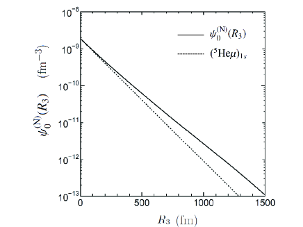
Figure 7: Amplitude $\psi_{0}^{({\rm N})}(R_{3})$ of the $(dt)$-$\mu$ relative motion in the nuclear-correlated term ${\widehat{\Phi}}_{0}^{({\rm N})}({\bf r}_{3},{\bf R}_{3})$ is represented by the solid curve, whereas the dotted curve represents the wave function of the $(^{5}{\rm He}\mu)_{1s}$ atom, $\propto e^{-R_{3}/a_{0}}$ with $a_{0}=131$ fm, normalized to $\psi_{0}^{({\rm N})}(R_{3})$ at $R_{3}=0$ for comparison. The solid curve is well simulated by the function $\propto e^{-R_{3}/a}$ with $a=154$ fm; this will be used in Eqs. (108) and (109). Here, the nuclear interactions of Set B is employed.

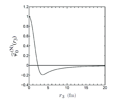
Figure 8: Amplitude of the $d$-$t$ relative motion ${\widehat{\varphi}}_{0}^{\,({\rm N})}(r_{3})$ in the nuclear-part wave function ${\widehat{\Phi}}_{0}^{({\rm N})}({\bf r}_{3},{\bf R}_{3})$ without the coupling of the $\alpha n\mu$ channel is illustrated by the solid curve. The curves have one node at $r_{3}\sim 2$ fm due to the orthogonality to the Pauli-forbidden (spurious) $0s$ wave function for the ⁵He nucleus of the $d$-$t$ potential model. Here, the nuclear interactions of Set B is employed.

Thus, we have reached a step closer to solving the coupled-channel Schrödinger equation (30) with the Coulomb force $V_{\alpha\mu}^{({\rm C})}(r_{5})$ omitted. As shown in Eqs. (35) and (36), the problem is deduced to solve the unknown functions $\varphi_{0}^{({\rm N})}(r_{3})$ and $\varphi_{2m}^{(+)}(k_{4},{\bf r}_{4})$. We expand $\varphi_{0}^{({\rm N})}(r_{3})$ in terms of the Gaussian basis functions in Eq. (40) with the parameters $(n_{\rm max},r_{1},r_{n_{\rm max}})=(20,0.5\,{\rm fm},20\,{\rm fm})$ as used in the case of ${\widehat{\varphi}}_{0}^{\,({\rm N})}(r_{3})$ in Eq. (46).

We rewrite $\varphi_{2m}^{(+)}(k_{4},{\bf r}_{4})$ as

$$\varphi^{(+)}_{2m}(k_{4},{\bf r}_{4})=\frac{u^{(+)}_{2}(k_{4},r_{4})}{r_{4}}\,Y_{2m}({\widehat{\bf r}}_{4})$$ (47)

and impose the outgoing boundary condition as

$$u^{(+)}_{2}(k_{4},r_{4})\stackrel{{\scriptstyle r_{4}\to\infty}}{{\longrightarrow}}\>S_{2}\,e^{ik_{4}r_{4}}.$$ (48)

The amplitude $S_{2}$ of the outgoing wave (48) is slightly different from the usual definition of $S$-matrix in the scattering with an incoming wave. In the present case, the dimension of $S_{2}$ is $L^{1}$ owing to the dimension $L^{-3}$ of the initial $(dt\mu)$ bound state $\mathring{\Phi}_{\frac{3}{2}M}^{({\rm C})}(dt\mu)$ in Eq. (26).

The flux of the $\alpha$-$n$ relative motion at $r_{4}\to\infty$ into the full direction ($4\pi$ sr) in a unit time is given as (note ${\widehat{\bf r}}_{4}={\widehat{\bf k}}_{4}$ )

$$v_{4}N_{\mu}\int\left|S_{2}\big{[}Y_{2}({\widehat{\bf k}_{4}})\chi_{\frac{1}{2}}(\alpha n)\big{]}_{\frac{3}{2}}\right|^{2}{\rm d}{\widehat{\bf k}}_{4}\,=v_{4}N_{\mu}|S_{2}|^{2}\>,\quad$$ (49)

where $v_{4}=\hbar k/\mu_{{\bf r}_{4}}$ is the velocity of the $\alpha$-$n$ relative motion, and $N_{\mu}$ is given by

$$N_{\mu}=\int|\,\psi_{0}^{({\rm N})}(R_{4})\,|^{2}\>{\rm d}{\bf R}_{4}.$$ (50)

The R.H.S. of Eq. (49) gives the fusion rate, namely, the number of $\alpha$-$n$ pair (number of muon) outgoing from one $(dt\mu)_{J=v=0}$ molecule:

$$\lambda_{\rm f}=v_{4}N_{\mu}|S_{2}|^{2}\,.\quad$$ (51)

III.2 Results

According to the above procedure, the coupled-channels Schrödinger equation (30) with the outgoing boundary condition (48) can be precisely solved by using the couple-channels Kohn-type variational method for composite-particle scattering Kamimura77 , which was used in Sec. II.

The $S$-matrix $S_{2}$ in Eq. (48) is obtained as

$$S_{2}=(0.5934+0.1985\,i)\>{\rm fm}.$$ (52)

Therefore, using $|S_{2}|^{2}=3.915\times 10^{-1}\,{\rm fm}^{2}$, $v_{4}=6.50\times 10^{22}\,{\rm fm\,s}^{-1}$ and $N_{\mu}=4.045\times 10^{-11}{\rm fm}^{-3}$ in Eq. (50), the calculated fusion rate is given as

$$\lambda_{\rm f}=1.03\times 10^{12}\>{\rm s}^{-1}.$$ (53)

This result is obtained by using the nuclear interaction Set B. Table II lists the fusion rates for three Sets A, B, and C; the rates imply that the present fusion-rate calculation is independent of the details of the employed nuclear interactions that reproduced the observed data in Figs. 4 and 5. Therefore, only Set B is used in Secs. V and VI.

A correction to $\lambda_{\rm f}$ owing to the $\alpha$-$\mu$ Coulomb potential, which is omitted when solving the Schrödinger equation, is discussed in Sec. VI A.

Table 2: Calculated fusion rate $\lambda_{\rm f}$ of $(dt\mu)_{J=v=0}$, Eq. (51), using the nuclear-interaction parameter sets A, B, and C in Table I.

		Set A		Set B		Set C
$\lambda_{\rm f}$ (s-1)		$1.03\times 10^{12}$		$1.03\times 10^{12}$		$1.02\times 10^{12}$

The above value of $\lambda_{\rm f}$ in (53) supports the literature results $\mbox{(1.0 - 1.3)}\times 10^{12}{\rm s}^{-1}$ (cf. Table 8 in the $\mu$CF review paper Froelich92 ) obtained in 1980’s - 90’s by using the $d$-$t$ optical-potential model Kamimura89 ; Bogdanova ; Bogdanova89 and by the $R$-matrix method Struensee88a ; Szalewicz90 ; Hale93 ; Hu1994 ; Cohen1996 ; Jeziorski91 .

It is found that $\varphi_{0}^{({\rm N})}(r_{3})$ is well simulated by

$$\varphi_{0}^{({\rm N})}(r_{3})\simeq(1.67+0.59\,i)\>{\widehat{\varphi}}_{0}^{\,({\rm N})}(r_{3}).$$ (54)

This enhancement in Eq. (54) by the $dt\mu$-$\alpha n\mu$ coupling will play an important role in the analysis in Secs. V and VI with the use of the $T$-matrix calculational method based on the Lippmann-Schwinger equation to be introduced in Sec. IV.

Figure 9 illustrates the three types of densities of the $d$-$t$ relative motion along ${\bf r}_{3}$;

$$\rho^{\rm(N)}(r_{3})\!\! = \!\!\!\int\big{|}\Phi_{0}^{({\rm N})}({\bf r}_{3},{\bf R}_{3})\big{|}^{2}\,{\rm d}{\bf R}_{3},$$ (55)

$${\widehat{\rho}}^{\rm(N)}(r_{3})\!\! = \!\!\!\int\big{|}{\widehat{\Phi}}_{0}^{({\rm N})}({\bf r}_{3},{\bf R}_{3})\big{|}^{2}\,{\rm d}{\bf R}_{3}$$ (56)

$${\mathring{\rho}}^{\rm(C)}(r_{3})\!\! = \!\!\!\int\big{|}{\mathring{\Phi}}_{0}^{({\rm C})}({\bf r}_{3},{\bf R}_{3})\big{|}^{2}\,{\rm d}{\bf R}_{3},$$ (57)

where the integration over the muon-coordinate ${\bf R}_{3}$ is performed. In Fig. 9, ${\mathring{\rho}}^{\rm(C)}(r_{3})$ multiplied by 100 is illustrated by the dashed curve for $r_{3}<10$ fm, whereas the inserted figure shows ${\mathring{\rho}}^{\rm(C)}(r_{3})$ for the entire region. The red curve gives $\rho^{\rm(N)}(r_{3})$ for the $d$-$t$ relative motion when all the nuclear interactions are employed. It should be emphasized that ${\mathring{\rho}}^{\rm(C)}(r_{3})$ is significantly smaller than $\rho^{\rm(N)}(r_{3})$ in the nuclear interaction region. Therefore, ${\mathring{\Phi}}_{0}^{({\rm C})}({\bf r}_{3},{\bf R}_{3})$ is expected to play a minor role compared to $\Phi_{0}^{({\rm N})}({\bf r}_{3},{\bf R}_{3})$ in the estimation of the $\alpha$-$\mu$ sticking and the ejected muon’s spectrum after the fusion; this will be discussed in detail in Secs. V and VI.

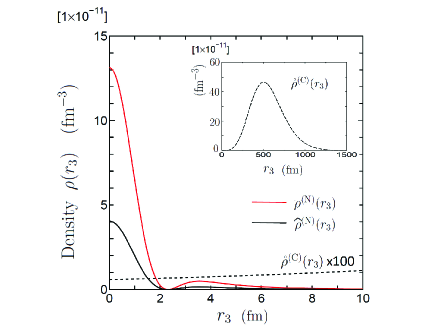
Figure 9: Three types of the densities of the $d$-$t$ relative motion associated with ${\bf r}_{3}$, which are defined in Eqs. (55)-(57). The dashed curve illutrates ${\mathring{\rho}}^{\rm(C)}(r_{3})$ multiplied by 100 for $r_{3}<10$ fm, whereas the entire behavior of ${\mathring{\rho}}^{\rm(C)}(r_{3})$ is given in the inserted figure. The red curve shows $\rho^{\rm(N)}(r_{3})$ for the nuclear part of the $d$-$t$ relative motion when the $dt\mu$-$\alpha n\mu$ coupling is switched on. The black solid curve for ${\widehat{\rho}}^{\rm(N)}(r_{3})$ represents the case for which the $dt\mu$-$\alpha n\mu$ coupling is switched off. We have $\int{\mathring{\rho}}^{\rm(C)}(r_{3})\,{\rm d}{\bf r}_{3}=1$ ($\langle\mathring{\Phi}_{0}^{({\rm C})}\,|\,\mathring{\Phi}_{0}^{({\rm C})}\rangle=1$), $\int\rho^{\rm(N)}(r_{3})\,{\rm d}{\bf r}_{3}=7.5\times 10^{-9}$ and $\int{\widehat{\rho}}^{\rm(N)}(r_{3})\,{\rm d}{\bf r}_{3}=2.4\times 10^{-9}$. Here, the nuclear interactions of Set B is used.

IV Use of Lippmann-Schwinger equation for $dt\mu$ fusion reaction

IV.1 $T$-matrix element

In this section, we propose the use of the Lippmann-Schwinger equation Lippmann as another method for studying the fusion reaction (2), in particular, to calculate the initial sticking of a muon to an $\alpha$ particle and the momentum and energy spectra of the emitted muon, respectively in Secs. V and VI.

Let’s suppose that the reaction from a plane-wave initial $\alpha$-channel is outgoing to the final $\beta$-channels assuming the following wave functions:

$$\mbox{Total wave function}:\Psi^{(+)}_{\alpha}(E_{\alpha}),$$

$$\mbox{Initial $\alpha$-channel wave function}:e^{i\,{\bf K}_{\alpha}\cdot{\bf R}_{\alpha}}\phi_{\alpha}(\xi_{\alpha}),$$

$$\mbox{Asymptotic form of final $\beta$-channel wave function}:$$

$$\quad f_{\beta\alpha}(\Omega_{\beta})\frac{e^{i\,K_{\beta}R_{\beta}}}{R_{\beta}}\,\phi_{\beta}(\xi_{\beta}),$$

where $\phi_{\alpha}(\xi_{\alpha})$ and $\phi_{\beta}(\xi_{\beta})$ are ortho-normalized intrinsic wave functions of the $\alpha$- and $\beta$-channels, respectively, and $f_{\beta\alpha}(\Omega_{\beta})$ is the scattering amplitude to be determined.

One can calculate the transition matrix elements $T_{\beta\alpha}$ from the well-known integral formula Lippmann ; Gell-Mann based on the Lippmann-Schwinger equation as

$$T_{\beta\alpha}=\langle\,e^{i\,{\bf K}_{\beta}\cdot{\bf R}_{\beta}}\phi_{\beta}(\xi_{\beta})\,|\,V_{\beta}\,|\,\Psi^{(+)}_{\alpha}(E_{\alpha})\,\rangle,$$ (58)

where $V_{\beta}$ is the interaction in the $\beta$-channel. Using this $T_{\beta\alpha}$, the $\beta$-channel asymptotic form of the total wave function $\Psi^{(+)}_{\alpha}(E_{\alpha})$ is written as

$$\langle\,\phi_{\beta}(\xi_{\beta})\,|\,\Psi^{(+)}_{JM}(E)\,\rangle\stackrel{{\scriptstyle R_{\beta}\to\infty}}{{\longrightarrow}}-\frac{\mu_{R_{\beta}}}{2\pi\hbar^{2}}\,T_{\beta\alpha}\,\frac{e^{iK_{\beta}R_{\beta}}}{R_{\beta}},$$ (59)

where $\mu_{R_{\beta}}$ is the reduced mass associated with ${\bf R}_{\beta}$. Therefore, we have

$$f_{\beta\alpha}(\Omega_{\beta})=-\frac{\mu_{R_{\beta}}}{2\pi\hbar^{2}}\,T_{\beta\alpha}\,.$$ (60)

The reaction cross section $\sigma_{\beta\alpha}$ is usually defined by the flux of the outgoing wave with a velocity $v_{\beta}(=\hbar K_{\beta}/\mu_{{\bf R}_{\beta}})$ into the full direction ($4\pi$ st) in a unit time divided by the flux of the incident wave $(=v_{\alpha})$ as

$$\!\!\!\sigma_{\beta\alpha}=\frac{v_{\beta}}{v_{\alpha}}\!\int|f_{\beta\alpha}(\Omega_{\beta})|^{2}\,{\rm d}\Omega_{\beta}=\frac{v_{\beta}}{v_{\alpha}}\left(\frac{\mu_{R_{\beta}}}{2\pi\hbar^{2}}\right)^{2}\!\!\int|T_{\beta\alpha}|^{2}\,{\rm d}{\widehat{\bf K}}_{\beta}.$$ (61)

The preceding expressions are exact provided that the total wave function $\Psi^{(+)}_{\alpha}(E_{\alpha})$ is rigorously exact. However, for typical reaction calculations, $\Psi^{(+)}_{\alpha}(E_{\alpha})$ in Eq. (58) is replaced by an approximate wave function.

In the present fusion reaction (2), however, the initial $\alpha$-channel is not the plane wave $e^{i\,{\bf K}_{\alpha}\cdot{\bf R}_{\alpha}}\phi_{\alpha}(\xi_{\alpha})$, but the $dt\mu$ bound state ${\mathring{\Phi}}_{\frac{3}{2}M}^{({\rm C})}(dt\mu)$ in Eq. (26). Therefore, in Eq. (61), we omit the incoming-channel information and replace the total wave function by our $\Psi_{\frac{3}{2}M}^{(+)}(E)$ of Eq. (26), and introduce the ‘reaction rate’, $r_{\beta\alpha}$, as

$$r_{\beta\alpha}=v_{\beta}\left(\frac{\mu_{R_{\beta}}}{2\pi\hbar^{2}}\right)^{2}\int|T_{\beta\alpha}|^{2}\,{\rm d}{\widehat{\bf K}_{\beta}}\,.$$ (62)

Since the initial-state wave function ${\mathring{\Phi}}_{\frac{3}{2}M}^{({\rm C})}(dt\mu)$ is normalized to unity (namely, starting with one molecule), $r_{\beta\alpha}$ represents the number (probability) of a molecule decaying into the $\beta$ channel per unit time. Therefore, the sum of $r_{\beta\alpha}$ over $\beta$ becomes the $T$-matrix expression of the fusion rate $\lambda_{\rm f}$:

$$\lambda_{\rm f}=\sum_{\beta}\;r_{\beta\alpha}\,.$$ (63)

Note that we call $r_{\beta\alpha}$ the reaction rate and $\lambda_{\rm f}$ the fusion rate throughout this work.

The definition of reaction rate $r_{\beta\alpha}$ is applied to the study of $\alpha$-$\mu$ sticking in Sec. V and to the momentum and energy spectra of the emitted muon in Sec. VI. In these applications, the fusion rates $\lambda_{\rm f}$ are calculated using $r_{\beta\alpha}$; these two types of additional calculations of the fusion rate should be consistent with the value already obtained in Eq. (53), which will be a significant test of the reliability of the present calculations.

IV.2 Discretization of two-body continuum states

In the definition of the $T$-matrix (58), $\phi_{\beta}(\xi_{\beta})$ are treated as ortho-normalized states. As the $\beta$-channel intrinsic states, however, we will consider the $\alpha$-$\mu$ continuum states associated with ${\bf r}_{5}$ (Sec. V) and the $\alpha$-$n$ continuum states associated with ${\bf r}_{4}$ (Sec. VI)

It is difficult to directly treat the continuum states in the $T$-matrix calculation. Instead, we discretize these states and construct the ortho-normalized discretized continuum states, such as ${\widetilde{\phi}}_{ilm}({\bf r}_{3})$ using $i$ to number the discretized states; we then consider their convergence back to the continuum. This discretization is performed by employing the CDCC (Continuum-Discretized-Coupled Channels) method that was developed by one of the present authors (M.K.) and his collaborators (for example, see review papers Kamimura86 ; Austern ; Yahiro12 ) for the study of projectile-breakup reactions. At present, this is one of the standard methods for investigating various reactions using light- and heavy-ion projectiles.

The discretization of continuum states is performed as follows: Let $\phi_{lm}(k,{\bf r})$ denote $k$-continuum states with angular-momentum $lm$ that satisfies the Schrödinger equation

$$\Big{[}-\frac{\hbar^{2}}{2\mu_{r}}\nabla^{2}_{r}+V(r)-\varepsilon\,\Big{]}\phi_{lm}(k,{\bf r})=0,\quad\varepsilon=\frac{\hbar^{2}\,k^{2}}{2\mu}.\quad$$ (64)

We confine the range of momentum as $0<k<k_{N}$ and divide it based on the interval $\mathit{\Delta}k_{i}=k_{i-1}-k_{i}\>(i=1,...,N)$; usually, $\mathit{\Delta}k_{i}$ is taken to be independent of $i$. We then take an average of the continuum wave functions in each momentum bin as

$${\widetilde{\phi}}_{ilm}({\bf r})=\frac{1}{\sqrt{\mathit{\Delta}k_{i}}}\int_{k_{i-1}}^{k_{i}}\!\!\phi_{lm}(k,{\bf r})\,dk,\;(i=1,...,N)$$ (65)

where the integration is performed numerically with the required accuracy.

Since $\phi_{lm}(k,{\bf r})$ is normalized as

$$\langle\,\phi_{lm}(k,{\bf r})\,|\,\phi_{lm}(k^{\prime},{\bf r})\,\rangle=\delta(k-k^{\prime}),$$ (66)

the discretized-continuum wave functions ${\widetilde{\phi}}_{ilm}({\bf r})$ have the ortho-normal relation

$$\langle\,{\widetilde{\phi}}_{ilm}({\bf r})\,|\,{\widetilde{\phi}}_{i^{\prime}lm}({\bf r})\rangle=\delta_{ii^{\prime}}.$$ (67)

Namely, ${\widetilde{\phi}}_{ilm}({\bf r})$ becomes an $L^{2}$-integrable function because of the cancelation between the asymptotic (oscillating) amplitudes of $\phi_{lm}(k,{\bf r})$ during the $k$-integration. A typical example of such a damping in the asymptotic region by averaging oscillating functions is as follows:

$$\int_{k_{i}}^{k_{i}+\mathit{\Delta}k_{i}}\!\!\!{\rm sin}\,kr\,dk=\frac{2\,{\rm sin}\frac{\mathit{\Delta}k_{i}}{2}r}{r}\,{\rm sin}\,(k_{i}\!+\!\frac{\mathit{\Delta}k_{i}}{2})r\,.$$ (68)

Each $\widetilde{\phi}_{ilm}$ can be regarded as if it were a discrete excited-state wave function with energy $\widetilde{\varepsilon}_{il}$ given by the expectation value of the Hamiltonian as

$$\widetilde{\varepsilon}_{i}=\frac{\hbar^{2}\,{\widetilde{k}}_{i}^{2}}{2\mu},\qquad{\widetilde{k}_{i}}^{2}=\Big{(}\frac{k_{i}+k_{i-1}}{2}\Big{)}^{2}+\frac{\mathit{\Delta}k_{i}^{2}}{12},\;$$ (69)

Convergence of the calculated results with $\mathit{\Delta}k_{i}\to 0$ is well discussed in review papers of the CDCC method Kamimura86 ; Austern ; Yahiro12 . Therefore, we can treat the $T$-matrix elements of three-body break-up systems similar to those of ‘two-body’ systems with many ‘discrete excited’ states.

V Muon sticking to $\alpha$ particle

After the fusion reaction (2) takes place, the emitted muon sticks to the $\alpha$ particle or goes to the $\alpha$-$\mu$ continuum states. The probability that this muon sticks to the bound state is referred to as the initial sticking probability, $\omega_{S}^{0}$, and is one of the most important parameters for determining fusion efficiency, since this muon is not available for further $\mu$CF cycles. However, as summarized in a previously published review paper Froelich92 , the $\alpha$-$\mu$ sticking is not yet completely understood.

In this section, we study the muon sticking problem in a much more sophisticated manner than that in the literature. We derive, for the first time, absolute values of the reaction (2) going to the $\alpha$-$\mu$ bound and continuum states. This is performed by calculating the $T$-matrix (58) for the reaction rate (62), in which the exact total wave function $\Psi^{(+)}_{\alpha}(E_{\alpha})$ is approximated by $\Psi_{\frac{3}{2}M}^{(+)}(E)$ of Eq. (26) that was already obtained by solving Schrödinger equation (30). In this Section, Set B is employed for the nuclear interactions.

V.1 $T$-matrix calculation of fusion rate

We calculate the $T$-matrix (58) for the reaction rate (62) of the fusion reaction

$$(dt\mu)_{J=v=0} \to (\alpha\mu)_{il}+n+17.6\,\mbox{MeV}$$ (70)

$$\searrow (\alpha\mu)_{nl}+n+17.6\,\mbox{MeV},$$

where $(\alpha\mu)_{nl}$ denotes the $n$-th $(\alpha\mu)$ bound state with $l$ presented by ${\phi}_{nlm}({\bf r}_{5})$ with the eigenenergy $\varepsilon_{nl}$, whereas $(\alpha\mu)_{il}$ describes the $i$-th discretized $\alpha$-$\mu$ continuum state that is obtained by discretizing $\phi_{lm}(k,{\bf r}_{5})$ into {${\widetilde{\varepsilon}}_{il},{\widetilde{\phi}}_{ilm}({\bf r}_{5}),i=1,...,N\}$ by performing Eqs. (65) and (69). We take $l=0$ to 25, $N=200$ and the maximum momentum $\hbar k_{N}=10\,{\rm MeV}/c$ ($\varepsilon_{N}\simeq 487$ keV) in this section.

In $T$-matrix (58), we replace the exact total wave function $\Psi^{(+)}_{\alpha}(E_{\alpha})$ by $\Psi_{\frac{3}{2}M}^{(+)}(E)$ that was given in Eq. (26) as the sum of the three components. Correspondingly, we divide the $T$-matrix (58) into three parts employing channel $c=5$ with the Jacobi coordinates $({\bf r}_{5},{\bf R}_{5})$ as

$$\!\!\!\!\!\!T^{({\rm C})}_{nl,mm_{s}}\!\!=\!\langle\,e^{i{\bf K}_{n}\cdot{\bf R}_{5}}\,\phi_{nlm}({\bf r}_{5})\chi_{\frac{1}{2}m_{s}}\!(n)\,|\,V^{({\rm T})}_{\alpha n,dt}\,|\mathring{\Psi}_{\frac{3}{2}M}^{({\rm C})}(dt\mu)\,\rangle,$$

$$\!\!\!\!\!\!T^{({\rm N})}_{nl,mm_{s}}\!\!=\!\langle\,e^{i{\bf K}_{n}\cdot{\bf R}_{5}}\,\phi_{nlm}({\bf r}_{5})\chi_{\frac{1}{2}m_{s}}\!(n)\,|\,V^{({\rm T})}_{\alpha n,dt}\,|\Psi_{\frac{3}{2}M}^{({\rm N})}(dt\mu)\,\rangle,$$

$$\!\!\!\!\!\!T^{(+)}_{nl,mm_{s}}\!\!=\!\langle\,e^{i{\bf K}_{n}\cdot{\bf R}_{5}}\,\phi_{nlm}({\bf r}_{5})\chi_{\frac{1}{2}m_{s}}\!(n)\,|\,V_{\alpha n}\,|\Psi_{\frac{3}{2}M}^{(+)}(\alpha n\mu)\,\rangle,$$

(71)

for the $\alpha$-$\mu$ bound states $\phi_{nlm}({\bf r}_{5})$ with the energy $\varepsilon_{nl}$, and

$$\!\!\!\!\!\!{\widetilde{T}}^{({\rm C})}_{il,mm_{s}}\!\!=\!\langle\,e^{i{\widetilde{\bf K}}_{i}\cdot{\bf R}_{5}}\,{\widetilde{\phi}}_{ilm}({\bf r}_{5})\chi_{\frac{1}{2}m_{s}}\!(n)\,|\,V^{({\rm T})}_{\alpha n,dt}\,|\mathring{\Psi}_{\frac{3}{2}M}^{({\rm C})}(dt\mu)\,\rangle,$$

$$\!\!\!\!\!\!{\widetilde{T}}^{({\rm N})}_{il,mm_{s}}\!\!=\!\langle\,e^{i{\widetilde{\bf K}}_{i}\cdot{\bf R}_{5}}\,{\widetilde{\phi}}_{ilm}({\bf r}_{5})\chi_{\frac{1}{2}m_{s}}\!(n)\,|\,V^{({\rm T})}_{\alpha n,dt}\,|\Psi_{\frac{3}{2}M}^{({\rm N})}(dt\mu)\,\rangle,$$

$$\!\!\!\!\!\!{\widetilde{T}}^{(+)}_{il,mm_{s}}\!\!=\!\langle\,e^{i{\widetilde{\bf K}}_{i}\cdot{\bf R}_{5}}\,{\widetilde{\phi}}_{ilm}({\bf r}_{5})\chi_{\frac{1}{2}m_{s}}\!(n)\,|\,V_{\alpha n}\,|\Psi_{\frac{3}{2}M}^{(+)}(\alpha n\mu)\,\rangle,$$

(72)

for the $\alpha$-$\mu$ discretized continuum states ${\widetilde{\phi}}_{ilm}({\bf r}_{5})$ with ${\widetilde{\varepsilon}}_{il}$.

In Eqs. (71) and (72), the plane-wave momenta ${\bf K}_{n}$ and ${\widetilde{\bf K}}_{i}$ are determined, respectively, as

$$\frac{\hbar^{2}}{2\mu_{R_{5}}}K_{n}^{2}=E_{00}+Q-{\varepsilon}_{nl},$$ (73)

$$\frac{\hbar^{2}}{2\mu_{R_{5}}}{\widetilde{K}}_{i}^{2}=E_{00}+Q-{\widetilde{\varepsilon}}_{i},\qquad{\widetilde{\varepsilon}}_{i}=\frac{\hbar^{2}}{2\mu_{r_{5}}}{\widetilde{k}}_{i}^{2}.\quad$$ (74)

The reaction rate (62) is written as

$$\!\!\!\!\!\!\!\!\!\!\!{r}_{nl}={v}_{nl}\left(\frac{\mu_{R_{5}}}{2\pi\hbar^{2}}\right)^{2}\!\sum_{m,m_{s}}\!\int\!\big{|}{T}^{({\rm C})}_{nl,mm_{s}}\!\!+\!{T}^{({\rm N})}_{nl,mm_{s}}\!\!+\!{T}^{(+)}_{nl,mm_{s}}\big{|}^{2}\,\!{\rm d}{\widehat{\bf K}_{n}},$$ (75)

$$\!\!\!\!\!\!\!\!\!\!\!{\widetilde{r}}_{il}={v}_{il}\left(\frac{\mu_{R_{5}}}{2\pi\hbar^{2}}\right)^{2}\!\sum_{m,m_{s}}\!\int\!\big{|}{\widetilde{T}}^{({\rm C})}_{il,mm_{s}}\!\!+\!{\widetilde{T}}^{({\rm N})}_{il,mm_{s}}\!\!+\!{\widetilde{T}}^{(+)}_{il,mm_{s}}\big{|}^{2}\,\!{\rm d}{\widehat{\widetilde{\bf K}}_{i}},$$ (76)

respectively, for the bound state $(nl)$ and for the discretized continuum state $(il)$. $v_{il}=\hbar{\widetilde{K}}_{i}/\mu_{R_{5}}$ is the velocity of the $(\alpha\mu)_{il}$-$n$ relative motion associated with ${\bf R}_{5}$, and similarly for ${v}_{nl}=\hbar K_{n}/\mu_{R_{5}}$. Since the reaction rates ${r}_{nl}\,({\widetilde{r}}_{il})$ do not depend on the $M$ ($z$-component of the total angular momentum $\frac{3}{2}$), it is not necessary to take the average with respect to $M$.

The components of the $T$-matrix elements are explicitly expressed to identify the dominant contribution to the reaction rates $r_{nl}({\widetilde{r}}_{il})$. This is a new approach for analyzing the initial sticking probability $\omega_{S}^{0}$ in Sec. V B.

We then transform the summation $\sum_{i}{\widetilde{r}}_{il}$ into the integration of a smooth continuum function $r_{l}(k)$ of $k$ as

$$\sum_{i=1}^{K_{N}}{\widetilde{r}}_{il}=\!\sum_{i=1}^{K_{N}}\Big{(}\frac{{\widetilde{r}}_{il}}{\mathit{\Delta}k}\Big{)}\mathit{\Delta}k\stackrel{{\scriptstyle\mathit{\Delta}k\to 0}}{{\longrightarrow}}\!\int_{0}^{k_{N}}\!r_{l}(k)\,{\rm d}k\equiv r_{l}^{\rm cont.}.\;$$ (77)

Test of this procedure is well explained in the review papers of the CDCC method Kamimura86 ; Austern ; Yahiro12

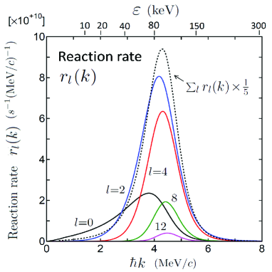
Figure 10: Calculated reaction rates ${r}_{l}(k)$ going to the $\alpha$-$\mu$ continuum states with the angular momentum $l$ defined in Eq. (77). The dotted black curve represents $\sum_{l=0}^{25}r_{l}(k)$ multiplied by $\frac{1}{5}$. The rates are given in units of ${\rm s}^{-1}({\rm MeV}/c)^{-1}$.

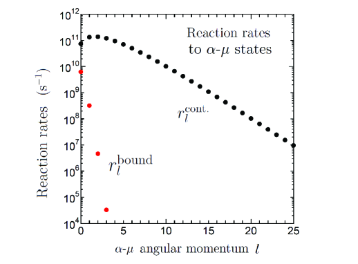
Figure 11: Calculated reaction rates $r_{l}^{\rm bound}$ (red circles) to the $\alpha$-$\mu$ bound states in Eq. (78) and $r_{l}^{\rm cont.}$ (black circles) to the $\alpha$-$\mu$ continuum states in Eq. (77) with respect to the angular momentum $l$. They are given in units of ${\rm s}^{-1}$.

The calculated reaction rates ${r}_{l}(k)$ are shown in Fig. 10 for angular momenta $l$ between $\alpha$ and $\mu$. The dotted black curve represents the summed rates $\sum_{l=0}^{25}\,r_{l}(k)$ multiplied by $\frac{1}{5}$. We see that the peak of the dotted curve is at $\hbar k\sim 4.3\,{\rm MeV}/c$ ($\varepsilon\sim 88$ keV). This is understood as follows: With the kinetic energy $3.5$ MeV (with speed $v_{\alpha}/c=0.043$), the $\alpha$ particle escapes from the muon cloud which has approximately the $(^{5}{\rm He}\mu)_{1s}$ wave function of ${\bf R}_{4}$. Conversely, the muon cloud is moving with respect to the $\alpha$ particle with the same speed $v_{\alpha}/c$, namely $\hbar k\sim 4.3$ MeV/c. The width of the peak of the dotted curve corresponds to the width of the momentum distribution within the muon cloud.

Furthermore, the reason why so many angular momenta $l$ appear in $r_{l}(k)$ in Fig. 11 is as follows: In the $T$-matrix elements (72), the component ’$|V|\Psi(dt\mu)\rangle$’ is composed of very short-range functions of ${\bf r}_{4}$ and long-range functions of ${\bf R}_{4}$. Therefore, many angular momenta $l$ are necessary to expand this unique function of $({\bf r}_{4},{\bf R}_{4})$ in terms of the functions $e^{i{\widetilde{\bf K}}_{i}\cdot{\bf R}_{5}}\,{\widetilde{\phi}}_{ilm}({\bf r}_{5})$ on the different Jacobi coordinates $({\bf r}_{5},{\bf R}_{5})$.

For comparison with $r_{l}^{\rm cont.}$ in Eq. (77), we introduce

$$r_{l}^{\rm bound}=\sum_{n}r_{nl}$$ (78)

for the transition to all the $\alpha$-$\mu$ bound states with $l$. Figure  11 illustrates how $r_{l}^{\rm bound}$ and $r_{l}^{\rm cont.}$ depend on the angular momentum $l$ of $0\leq l\leq 25$. $r_{l}^{\rm bound}$ are given by the red circles and $r_{l}^{\rm cont.}$ by the black ones. The rates $r_{l}^{\rm bound}$ decrease quickly with increasing $l$, whereas $r_{l}^{\rm cont.}$ changes slowly with respect to $l$. The ratio ($\sim 1\%$) of the strength of the red-circle group to that of the black-circle group is the essence of the initial $\alpha$-$\mu$ sticking probability, which is discussed in the next subsection.

Table 3: Fusion rates $\lambda_{\rm f}^{\rm cont.}$ and $\lambda_{\rm f}^{\rm bound}$ of the reaction $(dt\mu)_{J=v=0}\to(\alpha\mu)_{\rm cont.}+n\>$ or $\>(\alpha\mu)_{\rm bound}+n$, respectively, and their sum $\lambda_{\rm f}$, defined by Eqs. (79)-(80) on the Jacobi-coordinate channel $c=5$. Contribution to them from the full $T$-matrix and from the individual $T$-matrix elements $T^{({\rm C})},T^{({\rm N})}$ and $T^{(+)}$ are listed. The initial sticking probability $\omega_{S}^{0}(=\lambda_{\rm f}^{\rm bound}/\lambda_{\rm f})$ is given in the last line. Since the contribution from $T^{({\rm C})}$ and $T^{(+)}$ are minor, $\omega_{S}^{0}$ is not calculated there.

		$|T^{({\rm C})}\!+\!T^{({\rm N})}\!+\!T^{(+)}|^{2}$		$|T^{({\rm C})}|^{2}$		$|T^{({\rm N})}|^{2}$		$|T^{({\rm+})}|^{2}$
$\lambda_{\rm f}\,$ $({\rm s}^{-1})$		$8.05\times 10^{11}$		$3.70\times 10^{8}$		$7.73\times 10^{11}$		$1.18\times 10^{6}$
$\lambda_{\rm f}^{\rm cont.}$ $({\rm s}^{-1})$		$7.98\times 10^{11}$		$3.67\times 10^{8}$		$7.66\times 10^{11}$		$1.17\times 10^{6}$
$\lambda_{\rm f}^{\rm bound}$ $({\rm s}^{-1})$		$\!\!6.90\times 10^{9}$		$3.14\times 10^{6}$		$\!\!6.63\times 10^{9}$		$9.41\times 10^{3}$
$\omega_{S}^{0}\>(\%)$		$0.857$		—		$(0.857)$		—

Finally, we define the fusion rates to all the bound states and to all the continuum states, respectively as

$$\lambda_{\rm f}^{\rm bound}=\sum_{l=0}^{5}\>r_{l}^{\rm bound},\quad\lambda_{\rm f}^{\rm cont.}=\sum_{l=0}^{25}\>r_{l}^{\rm cont.}$$ (79)

and the sum of them as

$$\lambda_{\rm f} = \lambda_{\rm f}^{\rm bound}+\lambda_{\rm f}^{\rm cont.}.$$ (80)

This $\lambda_{\rm f}$ is the fusion rate of the reaction (2) defined by using the $T$-matrix in channel $c=5$.

In Table III, the calculated results of $\lambda_{\rm f},\lambda_{\rm f}^{\rm bound}$ and $\lambda_{\rm f}^{\rm cont.}$ are listed together with the contributions from the individual $T$-matrix elements $T^{({\rm C})},T^{({\rm N})}$ and $T^{(+)}$. We see that the fusion rate $\lambda_{\rm f}$ is obtained as

$$\lambda_{\rm f}=8.05\times 10^{11}\,{\rm s}^{-1}.$$ (81)

We consider that this value is consistent with $1.03\times 10^{12}\,{\rm s}^{-1}$ in Eq. (53) obtained by solving the couple-channels Schrödinger equation with the outgoing wave in channel $c\!=\!4$, taking into account the significant difference in the calculational methods and the fact that the $c\!=\!5$ channel component is not included in the total wave function $\Psi_{\frac{3}{2}M}^{(+)}(E)$.

Another important result in Table 3 is that the contribution to the fusion rates from $T^{({\rm C})}$ is much smaller than that from $T^{({\rm N})}$; this was expected from Fig. 9 since ${\mathring{\rho}}^{\rm(C)}(r_{3})$ is much smaller than $\rho^{\rm(N)}(r_{3})$ in the nuclear interaction region. This will be referred to in the next subsection for the $\alpha$-$\mu$ sticking probability $\omega_{S}^{0}$ .

V.2 Initial sticking probability $\omega_{S}^{0}$

The absolute values of the fusion rates $\lambda_{\rm f}^{\rm cont.}$ and $\lambda_{\rm f}^{\rm bound}$ have been explicitly calculated in the present three-body reaction calculation. This requires a change in the way of discussing the $\alpha$-$\mu$ sticking, as will be emphasized later.

Now, it is possible to calculate the initial muon-sticking probability by the definition

$$\omega_{S}^{0}=\frac{\lambda_{\rm f}^{\rm bound}}{\lambda_{\rm f}^{\rm bound}+\lambda_{\rm f}^{\rm cont.}}$$ (82)

that is based on the original idea for $\omega_{S}^{0}$ (cf., for example, Eq. (192) in Ref.  Froelich92 ), employing the nuclear interactions that reproduce the observation quantities in Figs. 4 and 5.

Before discussing our calculation of $\omega_{S}^{0}$, we review the essential point of previously reported studies on the $\alpha$-$\mu$ sticking probability referring to the review papers of $\mu$CF Ponomarev90 ; Froelich92 . Since the sudden approximation was used in the literature to define $\omega_{S}^{0}$, we first derive the same representation of their $\omega_{S}^{0}$ using our precise framework. We start from our definition (82) and make the following approximations i) to v):

i) In the $T$-matrix elements (71) and (72), the $\alpha n\mu$ outgoing wave $\Psi_{\frac{3}{2}M}^{(+)}(\alpha n\mu)$ is excluded from the total wave function $\Psi_{\frac{3}{2}M}^{(+)}(E)$ of (26). Omitting the spin component, the wave function of $(dt\mu)_{J=v=0}$ is represented by $\Phi_{0}^{(dt\mu)}({\bf r}_{3},{\bf R}_{3})$ that was obtained, for example in Ref. Kamimura89 , by diagonalizing the $dt\mu$ Hamiltonian (31). $\Phi_{0}^{(dt\mu)}({\bf r}_{3},{\bf R}_{3})$ is almost the same as $\mathring{\Phi}_{0}^{({\rm C})}({\bf r}_{3},{\bf R}_{3})\!+\!{\widehat{\Phi}}_{0}^{({\rm N})}({\bf r}_{3},{\bf R}_{3})$ obtained using the linear equation (44) (cf. Fig. 9).

ii) In Eqs. (71) and (72), the $dt$-$\alpha n$ transition interaction (33), $V^{({\rm T})}_{\alpha n,dt}$, is replaced as

$$\int d{\bf r}_{3}V_{dt,\alpha n}^{({\rm T})}({\bf r}_{3},{\bf r}_{4})\to V_{\delta}\!\!\,\int d{\bf r}_{3}\delta({\bf r}_{3})\,\delta({\bf r}_{4}),$$ (83)

which is the essence of the sudden approximation.

iii) The momentum ${\bf K}_{n}$ of the plane wave $e^{i{\bf K}_{n}\cdot{\bf R}_{5}}$ is fixed to ${\bf K}$ given by $\hbar^{2}K^{2}/2\mu_{R_{5}}=17.589$ MeV.

iv) The $T$-matrix elements and the fusion rates are given by

$$T_{nlm}=\langle\,e^{i{\bf K}\cdot{\bf R}_{5}}\,\phi_{nlm}({\bf r}_{5})|\,V_{\delta}\!\!\int\!{\rm d}{\bf r}_{3}\delta({\bf r}_{3})\delta({\bf r}_{4})|\,\Phi_{0}^{(dt\mu)}({\bf r}_{3},{\bf R}_{3})\rangle_{{\bf r}_{5},{\bf R}_{5}},$$

$$\qquad{=V_{\delta}\,\langle\,e^{i{\bf K}\cdot{\bf R}_{5}}\,\phi_{nlm}({\bf r}_{5})\,|\,\delta({\bf r}_{4})\,\Phi_{0}^{(dt\mu)}(0,{\bf R}_{4})\,\rangle_{{\bf r}_{5},{\bf R}_{5}},}$$

$$\qquad=V_{\delta}\,\langle\,e^{i{\bf q}\cdot{\bf r}_{5}}\,\phi_{nlm}({\bf r}_{5})|\,\Phi_{0}^{(dt\mu)}(0,{\bf r}_{5})\rangle_{{\bf r}_{5}},\quad$$ (84)

$$\lambda_{\rm f}^{\rm bound}=v\left(\frac{\mu_{R_{5}}}{2\pi\hbar^{2}}\right)^{2}\sum_{nlm}|T_{nlm}|^{2},\quad$$ (85)

$$\lambda_{\rm f}=v\left(\frac{\mu_{R_{5}}}{2\pi\hbar^{2}}\right)^{2}V_{\delta}^{2}\,\langle\Phi_{0}^{(dt\mu)}(0,{\bf r}_{5})|\,\Phi_{0}^{(dt\mu)}(0,{\bf r}_{5})\rangle_{{\bf r}_{5}},\quad\;\;$$ (86)

where ${\bf q}=\frac{m_{\mu}}{m_{\alpha}\!+\!m_{\mu}}{\bf K}$ and $v=\hbar K/\mu_{R_{5}}$. The completeness of the $\alpha$-$\mu$ basis functions {$\phi_{nlm}({\bf r}_{5}),\phi_{lm}(k,{\bf r}_{5})$} is used to derive $\lambda_{\rm f}$. The use of $\delta({\bf r}_{4})$ in Eq. (V.2) is based on the approximation that the nuclear interactions can be regarded as a contact interaction because the interaction range is much smaller than the muonic molecular size. This choice of the interaction, however, imposes $S$-wave for the $\alpha$-$n$ relative motion denoted with ${\bf r}_{4}$, which contradicts the observed fact of $D$-wave.

v) Finally, the sticking probability $\omega_{S}^{0}$ defined by (82) is approximated by ${\widehat{\omega}}_{S}^{0}$ as

$${\widehat{\omega}}_{S}^{0}=\frac{\sum_{nlm}|\,\langle\,e^{i{\bf q}\cdot{\bf r}_{5}}\,\phi_{nlm}({\bf r}_{5})|\,\Phi_{0}^{(dt\mu)}(0,{\bf r}_{5})\rangle_{{\bf r}_{5}}|^{2}}{\langle\,\Phi_{0}^{(dt\mu)}(0,{\bf r}_{5})|\,\Phi_{0}^{(dt\mu)}(0,{\bf r}_{5})\rangle_{{\bf r}_{5}}},$$ (87)

wherein no calculation is performed on the absolute values of $\lambda_{\rm f}^{\rm bound}$, $\lambda_{\rm f}^{\rm cont.}$ and $\lambda_{\rm f}$, since the $dt$-$\alpha n$ coupling interaction $V_{\delta}\!\int\!{\rm d}{\bf r}_{3}\delta({\bf r}_{3})\delta({\bf r}_{4})$ is not appropriate for the purpose.

We see that Eq. (87) is the same as the previous expression for $\omega_{S}^{0}$ under the sudden approximation (for example, see Eq. (207) of Ref. Froelich92 and Eq. (36) of Ref. Ponomarev90 ). Most of the literature calculations gave values in the region of

$${\widehat{\omega}}_{S}^{0}\simeq 0.88-0.89\%$$ (88)

without nuclear $d$-$t$ interactions (see the lines for ’Theory: Coulombic problem’ in Table 10 of the $\mu$CF review paper Froelich92 ). Similarly, with the nuclear $d$-$t$,

$${\widehat{\omega}}_{S}^{0}\simeq 0.91-0.93\%$$ (89)

were obtained by the optical-potential model Kamimura89 ; Bogdanova89 and the $R$-matrix method Struensee88a ; Szalewicz90 ; Hale93 ; Hu1994 ; Cohen1996 ; Jeziorski91 (In Refs. Hu1994 ; Cohen1996 ; Jeziorski91 , an internuclear distance $a_{dt}=0.51$ fm was taken in place of $r_{3}=a_{dt}=0$ in Eq. (87)). One of the present authors (M.K.) Kamimura89 participated in those calculations.

However, it should be noted that there is a serious problem in the discussion of ${\widehat{\omega}}_{S}^{0}$ in the case of (88) with the Coulomb force only for $\Phi_{dt\mu}({\bf r}_{3},{\bf R}_{3})$. This problem occurs because attention was not paid to the absolute values of $\lambda_{\rm f}^{\rm bound}$ and $\lambda_{\rm f}^{\rm cont.}$. This is made clear in Table 3 for $\lambda_{\rm f}^{\rm bound}$ and $\lambda_{\rm f}^{\rm cont.}$ together with their contributions from the three types of $T$-matrix, namely, $T^{({\rm C})},T^{({\rm N})}$ and $T^{(+)}$. The column $|T^{({\rm C})}|^{2}$ is responsible for the calculation of (88). We see that the contribution from $T^{({\rm C})}$ to $\lambda_{\rm f}^{\rm cont.}$ and $\lambda_{\rm f}^{\rm bound}$ is much smaller than that from $T^{({\rm N})}$; this is known from Fig. 9 since ${\mathring{\rho}}^{\rm(C)}(r_{3})$ is much smaller than $\rho^{\rm(N)}(r_{3})$ in the nuclear interaction region.

Therefore, we say that such a calculation of ${\widehat{\omega}}_{S}^{0}$ using the minor components of $\lambda_{\rm f}^{\rm cont.}$ and $\lambda_{\rm f}^{\rm bound}$ is not so meaningful (although it is useful when comparing the accuracy of the employed calculation methods with each other). In this sense, we placed the symbol ‘—’ in the column of $|T^{({\rm C})}|^{2}$ in the last line for $\omega_{S}^{0}$, and similarly in the column of $|T^{({\rm+})}|^{2}$. We also note that the statement “the additional effect of the nuclear force to the sticking probability” is not appropriate since $T^{({\rm N})}$ dominantly contributes to $\lambda_{\rm f}$ (Table 3), not additionally.

Our final result on the initial sticking probability is, as shown in the full $T$-matrix column of Table 3,

$$\omega_{S}^{0}=0.857\%\qquad\mbox{(present)},$$ (90)

which is reduced by $\sim 7\%$ from the value in (89). The origin of this reduction will be discussed in the next-to-last paragraph of Sec. V C.

Table 4 lists the calculated result of the muon initial sticking probability $\omega_{S}^{0}$ (%) of the $(dt\mu)_{J=v=0}$ state together with the $(\alpha\mu)_{nl}$-components. The last column is shown , only for reference, and is from our previous result in Ref. Kamimura89 based on the sudden approximation (87), in which the $d$-$t$ nuclear interaction is included but the $\alpha$-$n$ channel is not considered.

Table 4: The initial $\alpha$-$\mu$ sticking probability $\omega_{S}^{0}$ (%) of the (dt$\mu)_{J=v=0}$ state together with the $(\alpha\mu)_{nl}$-components. The present wave function includes the $\alpha n\mu$ channel with $D$-wave $\alpha$-$n$ relative motion. The last column is from our previous result Kamimura89 which employed the sudden approximation (87); the $d$-$t$ nuclear interaction was included but the $\alpha n\mu$ channel was not considered.

$J\!=\!v\!=\!0$		Present		Ref. Kamimura89
$\Psi_{\frac{3}{2}M}^{(+)}(\alpha n\mu)$		$\alpha$-$n\>D$ wave		No $\alpha$-$n$ wave
				(sudden approx.)
$\lambda_{\rm f}({\rm s}^{-1})$		$8.05\times 10^{12}$		$-$
$\lambda_{\rm f}^{{\rm bound}}({\rm s}^{-1})$		$6.90\times 10^{10}$		$-$
$\omega_{S}^{0}(\%)$		0.857		0.9261
$1s$		0.6583		0.7141
$2s$		0.0950		0.1021
$2p$		0.0233		0.0248
$3s$		0.0289		0.0310
$3p$		0.0084		0.0089
$3d$		0.0002		0.0002
$4s$		0.0123		0.0132
$4p$		0.0038		0.0040
$4d+4f$		0.0001		0.0001
$5s$		0.0063		0.0068
all others		0.0204		0.0208

V.3 Effective sticking probability $\omega_{S}^{\rm eff}$

Finally, we discuss the effective sticking probability $\omega_{S}^{\rm eff}$ that is defined as

$$\omega_{S}^{\rm eff}=\omega_{S}^{0}\,(1-R),$$ (91)

where $R$ is the muon reactivation coefficient that expresses the probability that the muon is shaken off from the $(\alpha\mu)_{nl}$ state during slowing down from the initial kinetic energy 3.5 MeV. The effective sticking $\omega_{S}^{\rm eff}$ is the most crucial parameter in the $\mu$CF cycle because it sets a limit on the maximum possible fusion output per muon.

Regarding the sticking problem, we understand as follows from Secs. 8.4-8.6 of the $\mu$CF review paper Froelich92 (1992): Using $R=0.287$ (for a low density $\phi=0.17$) of Ref. Stodden90 , the theoretical values of $\omega_{S}^{0}\simeq 0.91-0.93\%$ in (89) result in $\omega_{S}^{\rm eff}\sim 0.66\%$ , which is 10% larger than the experimental value $\omega_{S}^{\rm eff}=0.59\pm 0.07\%$ ($\phi=0.175$) at PSI Petitjean1990 (1991). Ref. Froelich92 states that the 10% difference is large enough to motivate further studies, because it may be a signal that the sticking problem is not yet completely understood.

In 2001, the final (last) precise experimental data on $\omega_{S}^{\rm eff}$ were reported from RIKEN-RAL Ishida2001 and PSI Petitjean2001 at high densities $(\phi=1.2-1.4)$. The results showed that

$$\omega_{S}^{\rm eff}=\begin{cases}\;0.532\pm 0.030\%\quad\text{({\rm Liquid}~{}\cite[cite]{\@@bibref{Authors Phrase1YearPhrase2}{Ishida2001}{\@@citephrase{(}}{\@@citephrase{)}}})},\\ \;0.515\pm 0.030\%\quad\text{({\rm Solid}~{}\cite[cite]{\@@bibref{Authors Phrase1YearPhrase2}{Ishida2001}{\@@citephrase{(}}{\@@citephrase{)}}})},\;\;\\ \;0.505\pm 0.029\%\quad\text{({\rm Liquid}~{}\cite[cite]{\@@bibref{Authors Phrase1YearPhrase2}{Petitjean2001}{\@@citephrase{(}}{\@@citephrase{)}}})}.\end{cases}$$ (92)

We derive our $\omega_{S}^{\rm eff}$ with the use of $\omega_{S}^{0}=0.857$ % in (90) and $R=0.35$ Struensee88b ; Stodden90 ; Markushin ; Rafelski for high densities (density dependence seems to be very small for $\phi\sim 1.2-1.5$ in Table VI of Ref. Stodden90 ). We obtain

$$\omega_{S}^{\rm eff}=0.557\%\qquad\mbox{(present)},$$ (93)

which can explain the observed values illustrated in Fig. 12, whereas the ${\widehat{\omega}}_{S}^{0}\simeq 0.91-0.93\%$ by the previous work gives $\omega_{S}^{\rm eff}\simeq 0.60$%.

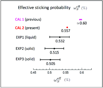
Figure 12: Comparison of the calculated effective sticking probability $\omega_{S}^{\rm eff}$ with the observed values based on from the precise high-density experiments EXP1 Ishida2001 , EXP2 Ishida2001 and EXP3 Petitjean2001 in 2001. CAL1 is given by the previous work with $\omega_{S}^{0}\simeq 0.91-0.93\%$ Kamimura89 ; Bogdanova89 ; Struensee88a ; Szalewicz90 ; Hale93 ; Hu1994 ; Cohen1996 ; Jeziorski91 , and CAL2 is owing to the present result with $\omega_{S}^{0}=0.857$ % of (90), with the definition $\omega_{S}^{\rm eff}=\omega_{S}^{0}(1-R)$ taking the reactivation coefficient as $R=0.35$ for high densities Struensee88b ; Stodden90 ; Markushin ; Rafelski .

To consider the origin of the change to $\omega_{S}^{0}=0.857$% in (90) from $0.91-0.93$% in (89), we perform an additional calculation in which the $\alpha$-$n$ outgoing $D$-wave is replaced by $S$-wave. This is performed only for a reference calculation since this change contradicts the observation that the outgoing $\alpha$-$n$ channel with $I^{\pi}=\frac{3}{2}^{+}$ has $D$-wave angular momentum.

We consider the following nonlocal central-force coupling, instead of the tensor force $V_{dt,\alpha n}^{({\rm T})}({\bf r}_{3},{\bf r}_{4})$ in Eq. (8):

$$V_{dt,\alpha n}^{({\rm S})}({\bf r}_{3},{\bf r}_{4}) \!\!\!=\!\!\! v_{0}^{(S)}\,e^{-\mu\,r_{34}^{2}-\mu^{\prime}R_{34}^{2}}$$ (94)

with $\mu=1/(1.0\,{\rm fm})^{2}$, $\mu^{\prime}=1/(6.0\,{\rm fm})^{2}$ and $v_{0}^{(S)}=0.81$ ${\rm MeV\,fm}^{-3}$ with a slight change to $V_{0}=-38.05\,$ MeV in the $d$-$t$ potential. The quality of the fitting to the observed $S$-factors is almost the same as the red curve in Fig. 4.

We have obtained $\lambda_{\rm f}\!=8.87\times 10^{11}\,{\rm s}^{-1}$ by solving the coupled-channels Schrödinger equation (30) and $\lambda_{\rm f}=7.56\times 10^{11}\,{\rm s}^{-1}$ by calculating the $T$-matrix elements (71) and (72); this result is not unreasonable. As for the $\alpha$-$\mu$ sticking problem, we see the change as follows:

$$\!\!\!\!\lambda_{\rm f,S{\rm-wave}}^{\rm bound}\!=7.09\times\!10^{9}{\rm s}^{-1}\to\lambda_{\rm f,D{\rm-wave}}^{\rm bound}\!=6.90\times\!10^{9}{\rm s}^{-1}$$

$$\!\!\!\!\lambda_{\rm f,S{\rm-wave}}^{\rm cont.}\!=7.49\times\!10^{11}{\rm s}^{-1}\!\!\to\lambda_{\rm f,D{\rm-wave}}^{\rm cont.}\!=7.98\times\!10^{11}{\rm s}^{-1},$$

which gives the change of $\omega_{S}^{0}=\lambda_{\rm f}^{\rm bound}/(\lambda_{\rm f}^{\rm bound}+\lambda_{\rm f}^{\rm cont.})$ from 0.938% ($S$-wave) to 0.857% ($D$-wave). Furthermore, we see that the former number of $\omega_{S}^{0}$ is close to that in (89) by the sudden approximation.

In conclusion, we have much improved the sticking-probability calculation by employing the $D$-wave $\alpha$-$n$ outgoing channel with the non-local tensor-force $dt$-$\alpha n$ coupling and by deriving the probability based on the absolute values of the $\lambda_{\rm f}^{\rm bound}$ and $\lambda_{\rm f}^{\rm cont.}$. The calculated result can reproduce the experimental value as mentioned above.

For more progress in the theoretical study of the effective sticking probability $\omega_{S}^{\rm eff}$, development of studying the reactivation coefficient $R$ is expected. Our result on the absolute values of the transition rates to the individual $(\alpha\mu)$ bound and continuum states in Table 4 and Fig. 10 will be useful.

VI Momentum and Energy spectra of emitted muon

In this section we calculate the momentum and energy spectra (in absolute values) of the emitted muon after the $dt\mu$ fusion (2). It is often stated that ‘10-keV’ muons are emitted during the reaction. However, it should be noted that 10 keV is the ‘average’ of the muon kinetic energy in the $({\rm He}\mu)_{1s}$ atom wherein the muon momentum distribution has a long higher-momentum tail. If one considers the utilization of such muons, for example, as the source of an ultra-slow negative muon beam Nagamine (1989); NagamineMCF199091 ; Strasser et al. (1993); Nagamine1996Hyp103 ; Strasser1996 ; Natori2020 ; Okutsu et al. (2021); Yamashita et al. (2021), it is important to determine the momentum and energy spectra of the released muon. In this Section, Set B is emplyed for the nuclear interactions.

For simplicity in expression, in this section, we refer to ${\bf K},{\bf K}_{i}$ and ${\widetilde{\bf K}}_{i}$ as ‘muon momentum’; more precisely, it is the momentum of the relative motion between the muon and the $\alpha$-$n$ pair; and similarly for ‘muon energy’ $E,E_{i}$ and ${\widetilde{E}}_{i}$.

To derive the momentum (energy) spectra as a continuous function of $K(E)$, prcise discretization of the momentum space both in the ($\alpha n)$-$\mu$ and the $\alpha$-$n$ relative motions is required while maintaining the energy conservation of the energy-sum of such motions. Such a correlated discretization is shown in Fig. 13. We start by assuming an upper limit of the muon momentum $K_{N}$ at the top of the left end of the figure, whereas the minimum momentum is $K_{0}=0$. We then divide the $K$-space $[K_{0},K_{N}]$ into $N$ bins ($K_{i},i=0-N$) with equal intervals $\mathit{\Delta}K$. Correspondingly, we divide the $k$-space $[k_{N},k_{0}]$ of the $\alpha$-$n$ relative motion on the right half of the figure into $N$ bins ($k_{i},i=0-N$) with the energy conservation kept as

$$E_{i}+\varepsilon_{i}=E_{00}+Q,\quad E_{i}=\frac{\hbar^{2}}{2\mu_{R_{4}}}K_{i}^{2},\quad\varepsilon_{i}=\frac{\hbar^{2}}{2\mu_{r_{4}}}k_{i}^{2},$$ (95)

where $K_{i}$ increases with increasing $i$, but $k_{i}$ decreases with increasing $i$. The bin width $\mathit{\Delta}\!K=K_{i}-K_{i-1}$ is constant in the left-half muon momentum space, whereas $\mathit{\Delta}k_{i}=|k_{i}-k_{i-1}|$ on the right half depends on $i$. Now, ${\widetilde{\phi}}_{ilm}({\bf r}_{4})$ is constructed using Eq. (65) but the $k$-integration runs from $k_{i}$ till $k_{i-1}$. The energy ${\widetilde{\varepsilon}}_{i}$ is given by Eq. (69). We take $N=200$ as the number of discretized momentum bins in Fig. 13, setting $\hbar K_{N}=6.0$  MeV/$c\,(E_{N}=175$ keV). This precise discretization is necessary for deriving the continuous muon $K(E)$-spectrum.

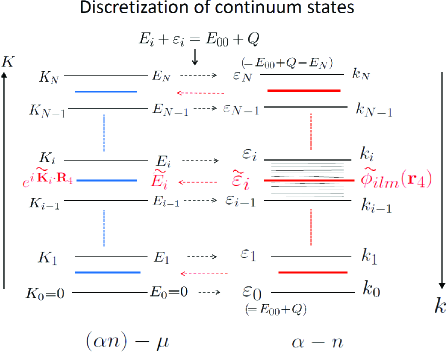
Figure 13: Schematic illustration for discretization of the momentum space $[K_{0},K_{N}]$ of the ($\alpha n$)-$\mu$ relative motion along ${\bf R}_{4}$ (left half) and that of the $\alpha$-$n$ relative motion $[k_{N},k_{0}]$ along ${\bf r}_{4}$ (right half) while maintaining $E_{i}+\varepsilon_{i}=E_{00}+Q$. The resulting discretized $\alpha$-$n$ continuum states ${\widetilde{\phi}}_{ilm}({\bf r}_{4})(i=1-N)$ are shown by the red lines and the associated muon plane waves $e^{i{\widetilde{\bf K}}_{i}\cdot{\bf R}_{4}}$ are represented by the blue lines in the left half. See text.

VI.1 $T$-matrix calculation of fusion rate

We calculate the muon spectra using the $T$-matrix procedure in Sec. VI A and the total wave function $\Psi_{\frac{3}{2}M}^{(+)}(E)$ that was already obtained in Sec. III as the sum of three components (cf. Eq. (26)). Correspondingly, as in Sec. V A, we divide the $T$-matrix (58) into three components on the Jacobi coordinates $({\bf r}_{4},{\bf R}_{4})$ in channel $c=4$ (cf. Fig. 3) as

$$\!\!\!\!\!\!{T}^{({\rm C})}_{il,mm_{s}}\!\!=\!\langle\,e^{i{\widetilde{\bf K}}_{i}\cdot{\bf R}_{4}}\,{\widetilde{\phi}}_{ilm}({\bf r}_{4})\chi_{\frac{1}{2}m_{s}}\!(n)\,|\,V^{({\rm T})}_{\alpha n,dt}\,|\mathring{\Psi}_{\frac{3}{2}M}^{({\rm C})}(dt\mu)\,\rangle,$$

$$\!\!\!\!\!\!{T}^{({\rm N})}_{il,mm_{s}}\!\!=\!\langle\,e^{i{\widetilde{\bf K}}_{i}\cdot{\bf R}_{4}}\,{\widetilde{\phi}}_{ilm}({\bf r}_{4})\chi_{\frac{1}{2}m_{s}}\!(n)\,|\,V^{({\rm T})}_{\alpha n,dt}\,|\Psi_{\frac{3}{2}M}^{({\rm N})}(dt\mu)\,\rangle,$$

$$\!\!\!\!\!\!{T}^{(+)}_{il,mm_{s}}\!\!=\!\langle\,e^{i{\widetilde{\bf K}}_{i}\cdot{\bf R}_{4}}\,{\widetilde{\phi}}_{ilm}({\bf r}_{4})\chi_{\frac{1}{2}m_{s}}\!(n)\,|\,V_{\alpha\mu}\,|\Psi_{\frac{3}{2}M}^{(+)}(\alpha n\mu)\,\rangle,$$ (96)

where ${\widetilde{\phi}}_{ilm}({\bf r}_{4})\,(i=1-N)$ is the discretized $\alpha$-$n$ continuum state with energy $\widetilde{\varepsilon}_{il}$, and $e^{i{\widetilde{\bf K}}_{i}\cdot{\bf R}_{4}}$ is the associated $(\alpha n)$-$\mu$ plane wave, satisfying the energy conservation

$$\qquad\quad{\widetilde{E}}_{i}+{\widetilde{\varepsilon}}_{i}=E_{00}+Q\qquad(i=1-N).$$ (97)

The third component $T^{(+)}$ of (96) estimates the effect of the Coulomb potential $V_{\alpha\mu}(r_{5})$ on the $T$-matrix. Here, we note that it is not necessary to use the Coulomb wave function, instead of the plane wave, in the bra-vector of the above $T$-matrix elements; the reason is explained in Appendix.

The reaction rate (62) for a muon emitted to the discretized continuum state $(\alpha n)_{il}$-$\mu$ is written as

$$\!\!\!{r}_{il}={v}_{il}\left(\frac{\mu_{R_{4}}}{2\pi\hbar^{2}}\right)^{2}\sum_{m,m_{s}}\int\big{|}{T}^{({\rm C})}_{il,mm_{s}}+{T}^{({\rm N})}_{il,mm_{s}}+{T}^{(+)}_{il,mm_{s}}\big{|}^{2}\,{\rm d}{\widehat{\widetilde{\bf K}}}_{i},$$ (98)

where ${v}_{il}=\hbar{\widetilde{K}}_{i}/\mu_{R_{4}}$ is the velocity of the $(\alpha n)_{il}$-$\mu$ relative motion. Since ${r}_{il}$ does not depend on the $M$ ($z$-component of the total angular momentum $\frac{3}{2}$), it is not necessary to take the average with respect to $M$. The sum of the transition rates

$$\lambda_{\rm f}=\sum_{il}\;{r}_{il}$$ (99)

is the fusion rate of the reaction (2) using the $T$-matrix based on channel $c=4$. This $\lambda_{\rm f}$ is compared with the $\lambda_{\rm f}$ obtained in Secs. II B and V C using different prescriptions.

To investigate the role of the three types of $T$-matrix elements in Eq. (98), we calculate the individual reaction rates

$$\lambda_{\rm f}^{\rm(C)}=\sum_{il}\;{r}_{il}^{\rm(C)},\quad{r}_{il}^{({\rm C})}={v}_{il}\left(\frac{\mu_{R_{4}}}{2\pi\hbar^{2}}\right)^{2}\sum_{m,m_{s}}\int\big{|}{T}^{({\rm C})}_{il,mm_{s}}\big{|}^{2}\,{\rm d}{\widehat{\widetilde{\bf K}}}_{i}\,,$$

$$\lambda_{\rm f}^{\rm(N)}=\sum_{il}\;{r}_{il}^{\rm(N)},\quad{r}_{il}^{({\rm N})}={v}_{il}\left(\frac{\mu_{R_{4}}}{2\pi\hbar^{2}}\right)^{2}\sum_{m,m_{s}}\int\big{|}{T}^{({\rm N})}_{il,mm_{s}}\big{|}^{2}\,{\rm d}{\widehat{\widetilde{\bf K}}}_{i}\,,$$

$$\lambda_{\rm f}^{\rm(+)}=\sum_{il}\;{r}_{il}^{\rm(+)},\quad{r}_{il}^{(+)}={v}_{il}\left(\frac{\mu_{R_{4}}}{2\pi\hbar^{2}}\right)^{2}\sum_{m,m_{s}}\int\big{|}{T}^{({\rm+})}_{il,mm_{s}}\big{|}^{2}\,{\rm d}{\widehat{\widetilde{\bf K}}}_{i}\,.$$

(100)

In the calculation of the $\lambda_{\rm f}^{({\rm C})}$ and $\lambda_{\rm f}^{({\rm N})}$, the contribution from the final states ${\widetilde{\phi}}_{ilm}({\bf r}_{4})$ with $l\neq 2$ is negligible under the $dt$-$\alpha n$ tensor coupling interaction. In $\lambda_{\rm f}^{({\rm+})}$ for the $\alpha$-$\mu$ Coulomb force effect, the contribution from $l>4$ is negligible.

The calculated fusion rate $\lambda_{\rm f}$ and the individual contributions $\lambda_{\rm f}^{\rm(C)},\lambda_{\rm f}^{\rm(N)}$ and $\lambda_{\rm f}^{\rm(+)}$ are listed in Table 5. Finally, we obtain the full fusion rate as

$$\lambda_{\rm f}=1.15\times 10^{12}\,{\rm s}^{-1}.$$ (101)

From $\lambda_{\rm f}^{({\rm C})}$ and $\lambda_{\rm f}^{({\rm N})}$ in Table 5, it is observed that a fusion reaction occurs mostly from $\Psi_{\frac{3}{2}M}^{({\rm N})}(dt\mu)$, whereas the contribution from $\mathring{\Psi}_{\frac{3}{2}M}^{({\rm C})}(dt\mu)$ is minor; this was already expected based on Fig. 9 since ${\mathring{\rho}}^{\rm(C)}(r_{3})$ is much smaller than $\rho^{\rm(N)}(r_{3})$ in the nuclear interaction region.

The term $T^{({\rm+})}$ describes the effect of the Coulomb force that acts on the $\alpha$ and $\mu$ in the outgoing $\alpha n\mu$ channel. This force was omitted when solving the Schrödinger equation (30); however, this approximation is corrected via the $T$-matrix calculation presented in this subsection. The correction was obtained as $\lambda_{\rm f}-\lambda_{\rm f}^{({\rm N})}=0.11\times 10^{12}\,{\rm s}^{-1}$. Therefore, the final result of the fusion rate in this study is expressed as Eq. (101), $1.15\times 10^{12}\,{\rm s}^{-1}$.

Table 5: Fusion rate $\lambda_{\rm f}$ (in units of ${\rm s}^{-1}$) calculated by (99) and individual rates $\lambda_{\rm f}^{({\rm C})}$, $\lambda_{\rm f}^{({\rm N})}$, and $\lambda_{\rm f}^{({\rm+})}$ by (100) on the Jacobi-coordinate channel $c=4$. The second line shows the type of used $T$-matrix.

$\lambda_{\rm f}$		$\lambda_{\rm f}^{({\rm C})}$		$\lambda_{\rm f}^{({\rm N})}$		$\lambda_{\rm f}^{({\rm+})}$
$|T^{({\rm C})}\!+\!T^{({\rm N})}\!+\!T^{(+)}|^{2}$		$|T^{({\rm C})}|^{2}$		$|T^{({\rm N})}|^{2}$		$|T^{({\rm+})}|^{2}$
$1.15\times 10^{12}$		$4.58\times 10^{8}$		$1.04\times 10^{12}$		$1.80\times 10^{11}$

It should be noted that, in some cases, the calculation of $T$-matrix elements for the Coulomb force between the continuum states is hindered by a problem in the integration up to the infinity. However, this issue is circumvented in the present work since we employ the discretization of the continuum states then smooth it as done in Eqs. (103) and (104).

Here, it is to be emphasized that both the solution of the Schrödinger equation and the calculation of $T$-matrix elements are very accurate in the case wherein the Coulomb force $V_{\alpha\mu}^{({\rm C})}(r_{5})$ is omitted. The reason is as follows: As shown in Sec. IV, provided that the total wave function $\Psi_{\frac{3}{2}M}^{(+)}(E)$ obtained by solving the Schrödinger equation is exact, the asymptotic behavior exhibited by the $T$-matrix calculation is the same as that given by $\Psi_{\frac{3}{2}M}^{(+)}(E)$. In the present case, the fusion rate $\lambda_{\rm f}$ was obtained as $1.04\times 10^{12}\,{\rm s}^{-1}$ by the $T$-matrix calculation (cf. the case $|T^{({\rm C})}\!+\!T^{({\rm N})}|^{2}\simeq|T^{({\rm N})}|^{2}$ in Table 5) and as $1.03\times 10^{12}\,{\rm s}^{-1}$ using the $S$-matrix of $\Psi_{\frac{3}{2}M}^{(+)}(E)$ (cf. Eq.(53)).

VI.2 Muon spectrum

The aim of this Sec. VI is to calculate the muon momentum and energy spectra as continuous functions of $K$ and the kinetic energy $E$, respectively. Here, $K(E)$ is the momentum (kinetic energy) of the $(\alpha n)$-$\mu$ relative motion associated with ${\bf R}_{4}$, whereas the muon momentum $K_{\mu}$ (kinetic energy $E_{\mu}$) measured from the center of mass of the $\alpha n\mu$ system is given by

$$K_{\mu}=K,\quad\quad E_{\mu}=\gamma E,\quad$$ (102)

with $\gamma=\frac{m_{\alpha}+m_{n}}{m_{\alpha}+m_{n}+m_{\mu}}=0.9779$. We note that the center of mass of the $\alpha n\mu$ is almost at rest in the laboratory system since the $(dt\mu)$ molecule is also almost at rest at the fusion (2).

The momentum spectra $r(K)$ and $r^{({\rm N})}(K)$ can be obtained, by smoothing ${r}_{il}$ and ${r}_{il}^{({\rm N})}$, respectively, as

$$\!\!\!\!\lambda_{\rm f}=\sum_{il}\Big{(}\frac{{r}_{il}}{\mathit{\Delta}\!K}\Big{)}\,\mathit{\Delta}\!K\stackrel{{\scriptstyle\mathit{\Delta}\!K\to 0}}{{\longrightarrow}}\int_{0}^{K_{N}}\!r(K)\,{\rm d}K,$$ (103)

$$\!\!\!\!\lambda_{\rm f}^{({\rm N})}=\sum_{il}\Big{(}\frac{{r}^{({\rm N})}_{il}}{\mathit{\Delta}\!K}\Big{)}\,\mathit{\Delta}\!K\stackrel{{\scriptstyle\mathit{\Delta}\!K\to 0}}{{\longrightarrow}}\int_{0}^{K_{N}}\!r^{({\rm N})}(K)\,{\rm d}K,\qquad$$ (104)

and similarly for $r^{({\rm C})}(K)$ and $r^{({\rm+})}(K)$.

Figure 14: Momentum spectrum of the muon emitted by the $dt\mu$ fusion. The red and black curves denote ${r}(K)$ and ${r}^{({\rm N})}(K)$ defined in (103) and (104), respectively. The dotted curve shows $r^{({\rm N})}_{\rm AD}(K)$ by the adiabatic approximation for $r^{({\rm N})}(K)$ (see text); $r^{({\rm N})}_{\rm AD}(K)$ is normalized to $r^{({\rm N})}(K)$ to have the same $K$-integrated values, $\lambda_{\rm f}^{\rm(N)}=1.04\times 10^{12}\,{\rm s}^{-1}$.

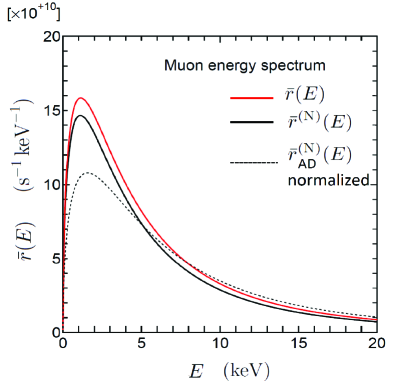
Figure 15: Energy spectrum of the muon emitted during the $dt\mu$ fusion. The red and black curves denote ${\bar{r}}(E)$ and ${\bar{r}}^{({\rm N})}(E)$ defined in (105) and (106), respectively. The peak position is at $E=1.1$ keV in the two cases. The dotted curve shows ${\bar{r}}^{({\rm N})}_{\rm AD}(E)$ obtained using the adiabatic approximation for ${\bar{r}}^{({\rm N})}(E)$ (see text); ${\bar{r}}^{({\rm N})}_{\rm AD}(E)$ is normalized to ${\bar{r}}^{({\rm N})}(E)$ to have the same $E$-integrated values, $\lambda_{\rm f}^{\rm(N)}=1.04\times 10^{12}\,{\rm s}^{-1}$.

The energy spectra ${\bar{r}}(E)$ and ${\bar{r}}^{({\rm N})}(E)$ are derived, with the use of $E=\hbar^{2}K^{2}/2\mu_{{\rm R}_{4}}$, by

$${\bar{r}}(E)\,{\rm d}E=\!\!\!\! r(K)\,{\rm d}K,$$ (105)

$${\bar{r}}^{({\rm N})}(E)\,{\rm d}E=\!\!\!\! r^{({\rm N})}(K)\,{\rm d}K,$$ (106)

and similarly for ${\bar{r}}^{({\rm C})}(E)$ and ${\bar{r}}^{({\rm+})}(E)$.

The calculated momentum spectrum $r(K)$ is illustrated in Fig. 14 by the red curve in units of ${\rm s}^{-1}({\rm MeV}/c)^{-1}$, whereas $r^{({\rm N})}(K)$ is represented by the black curve. The energy spectrum ${\bar{r}}(E)$ is shown in Fig. 15 by the red curve in units of ${\rm s}^{-1}({\rm keV})^{-1}$, whereas ${\bar{r}}^{({\rm N})}(E)$ is represented by the black curve.

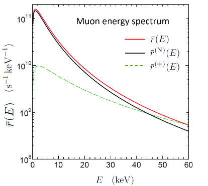
Figure 16: Energy spectrum of the muon emitted during the $dt\mu$ fusion in log scale. The red and black curves denote ${\bar{r}}(E)$ and ${\bar{r}}^{({\rm N})}(E)$ defined in (105) and (106), respectively. The dotted green curve represents ${\bar{r}}^{({\rm+})}(E)$ when only $|{T}^{(+)}|^{2}$ is used.

The difference between the red and black curves in Figs. 14 and 15 originates from the $\alpha$-$\mu$ Coulomb-force contribution $T^{({\rm+})}$ in Eq. (98). The contribution from $T^{({\rm C})}$ is minor. The effect of $T^{({\rm+})}$ is small at low energies but becomes relatively large at high energies, which is seen in Fig. 16 for the log scale, in the dotted green curve derived based on only $|T^{(+)}|^{2}$.

Table 6: Property of the energy spectrum of muon emitted from $(dt\mu)_{J=v=0}\to\alpha+n+\mu$ given by the present calculation, ${\bar{r}}(E)$ and ${\bar{r}}^{({\rm N})}(E)$, and the adiabatic approximation ${\bar{r}}^{({\rm N})}_{\rm AD}(E)$ which gives no absolute value (cf. Fig. 15).

Muon energy spectrum		Peak		Average		Peak
		energy		energy		strength
		(keV)		(keV)		$({\rm s}\cdot{\rm keV})^{-1}$
Present, ${\bar{r}}(E)$		1.1		9.5		$1.60\times 10^{11}$
Present, ${\bar{r}}^{({\rm N})}(E)$		1.1		8.5		$1.47\times 10^{11}$
Adiabatic, ${\bar{r}}^{({\rm N})}_{\rm AD}(E)$		1.6		10.9		$-$

As shown in Fig. 15 and Table 6, the peak of the energy spectrum is located at $E=1.1$ keV both for ${\bar{r}}(E)$ and ${\bar{r}}^{\rm(N)}(E)$. Since the spectrum has a long high-energy tail, the average energy is $9.5$ keV $(8.5$ keV) for ${\bar{r}}(E)\,({\bar{r}}^{\rm(N)}(E))$. Therefore, ‘muons with 1-keV peak energy and 10-keV average energy’ are emitted by the $dt\mu$ fusion. This result (more precisely, Figs. 14 and 15) will be useful for the ongoing experimental project to realize an ultra-slow negative muon beam using the $\mu$CF Nagamine (1989); NagamineMCF199091 ; Strasser et al. (1993); Strasser1996 ; Nagamine1996Hyp103 ; Natori2020 (cf. Type II of Sec. I).

When the authors of Refs.Nagamine (1989); NagamineMCF199091 ; Nagamine1996Hyp103 proposed the solid D-T layer system that cools the incident muon beam by utilizing the $\mu$CF, they used the calculated muon energy spectrum in Fig. 1 of Ref. Mueller , wherein the spectrum was represented by a shape that was set to unity at $E=0$. However, the definition of this energy spectrum is different from our energy spectrum ${\bar{r}}(E)\,(=0$ at $E=0$) that is represeted in absolute value and $\int_{0}^{\infty}\bar{r}(E){\rm d}E$ gives the fusion rate $\lambda_{\rm f}=1.15\times 10^{12}{\rm s}^{-1}$. The role of the $\alpha$-$\mu$ Coulomb force, which was discussed in Ref. Mueller by using their convoy-muon approximation, is properly included in our formulation via the $T$-matrix $T^{(+)}$.

For the sake of the observation of the muon energy spectrum, we present a cumulative distribution function, $P(E_{\rm x})$, associated with the muon energy spectrum ${\bar{r}}(E)$, defined by

$$P(E_{\rm x})=\frac{\int_{0}^{E_{\rm X}}\,{\bar{r}}(E)\,{\rm d}E}{\int_{0}^{\infty}\,{\bar{r}}(E)\,{\rm d}E}\leq 1\>,$$ (107)

which is illustrated by the red curve in Fig. 17. The dotted black curve is for $P(E_{\rm x})$ calculated with the adiabatic approximation, namely using ${\bar{r}}^{({\rm N})}_{\rm AD}(E)$ instead of ${\bar{r}}(E)$ in Eq. (107). Here, absolute value of the energy spectrum is not concerned.

The red curve indicates that 24 % of the emitted muon is in the region $0<E<2$ keV and 35% is in $0<E<3$ keV, and hence 11% is from $2<E<3$ keV, whereas the muon having $0<E<4.7$ keV is 50% and the one with $0<E<10$ keV amounts to 75%. The curve reaches 99% when $E_{\rm x}=80$ keV.

Figure 17: Cumulative distribution function $P(E_{\rm x})$ associated with the muon energy spectrum ${\bar{r}}(E)$. $P(E_{\rm x})$ is defined by Eq. (107). The red curve is derived by integrating ${\bar{r}}(E)$ of Fig. 15, whereas the dotted curve is given by using ${\bar{r}}^{({\rm N})}_{\rm AD}(E)$ instead of ${\bar{r}}(E)$.

It is found that the ‘shape’ of the two black curves for $r^{({\rm N})}(K)$ and ${\bar{r}}^{({\rm N})}(E)$ in Figs. 14 and 15, respectively, are well simulated by simple functions as

$$r^{\rm(N)}(K)\propto\frac{K^{2}}{(1+K^{2}a^{2})^{4}},\quad$$ (108)

$${\bar{r}}^{\rm(N)}(E)\propto\frac{K}{(1+K^{2}a^{2})^{4}},\quad E=\hbar^{2}K^{2}/2\mu_{{\rm R}_{4}}\qquad$$ (109)

with $a=154$ fm (this number appeared in Fig. 7). The reason is as follows: Using the property (34) of ${\widehat{\Phi}}_{0}^{({\rm N})}({\bf r}_{3},{\bf R}_{3})$, we can represent the $T$-matrix (96), without the spin part, as

$$\!\!\!\!\!T_{il,m}^{({\rm N})}\!=\!\langle{\widetilde{\phi}}_{ilm}({\bf r}_{4})|V^{({\rm T})}({\bf r}_{4},{\bf r}_{3})|\,\varphi^{({\rm N})}_{0}({\bf r}_{3})\rangle\langle e^{i{\bf{\widetilde{K}}_{i}}\cdot{\bf R}_{4}}\,|\,\psi^{({\rm N})}_{0}({\bf R}_{4})\rangle.\;$$ (110)

Taking $E_{N}\approx 0.2\,{\rm MeV}\ll Q$ and the relations (cf. Fig. 13)

$$Q-E_{N}\leq\varepsilon_{i}\leq Q\;\;\;({\rm namely,}\;\varepsilon_{i}\approx Q,\>k_{i}\approx k_{0})$$ (111)

together with Eq. (95), we can derive

$$\mathit{\Delta}k_{i}\approx\frac{\mu_{r_{4}}}{\mu_{R_{4}}}\frac{K_{i}}{k_{0}}\mathit{\Delta}\!K\propto{K_{i}}.$$ (112)

We then obtain, in the interaction region of $V^{({\rm T})}({\bf r}_{4},{\bf r}_{3})$,

$$\!\!\!\!\!\!\!{\widetilde{\phi}}_{ilm}({\bf r}_{4})\!\!\!\!\! =\frac{1}{\sqrt{\mathit{\Delta}k_{i}}}\int_{k_{i}}^{k_{i-1}}\!\!\phi_{lm}(k,{\bf r}_{4})\,{\rm d}k\approx\!\sqrt{\mathit{\Delta}k_{i}}\,\phi_{lm}(k_{i},{\bf r}_{4})$$ (113)

$$\approx\sqrt{\mathit{\Delta}k_{i}}\,\phi_{lm}(k_{0},{\bf r}_{4})\propto\!\sqrt{K_{i}}\,\phi_{lm}(k_{0},{\bf r}_{4}).$$

Substituting this ${\widetilde{\phi}}_{ilm}({\bf r}_{4})$ into Eq. (110) and smoothing ${\bf K}_{i}$ and ${\bf{\widetilde{K}}_{i}}$ to ${\bf K}$, we finally obtain (note $v_{il}\propto{\widetilde{K}}_{i}$)

$$r^{({\rm N})}(K)\propto K^{2}\!\!\int\!\!\,\big{|}\langle\,e^{i{\bf K}\cdot{\bf R}_{4}}\,|\,\psi^{({\rm N})}_{0}({\bf R}_{4})\rangle\big{|}^{2}{\rm d}{\widehat{\bf K}}.$$ (114)

As shown in Fig. 7 (note ${\bf R}_{4}={\bf R}_{3}$), $\psi_{0}^{({\rm N})}(R_{4})$ is well represented by $\propto e^{-R_{4}/a}$ with $a=154$ fm. Putting this function form into Eq. (114), we immediately obtain Eq. (108), from which we have Eq. (109) with Eq. (106). We found that both of the simulated functions well reproduce the corresponding black solid curves in Figs. 14 and 15 within the width of the curves under the normalization at the peaks.

Finally, we discuss the muon momentum and energy spectra if we take the adiabatic approximation for the $d$-$t$ relative motion just before the fusion reaction occurs. In this case, the wave function of the $(dt)$-$\mu$ relative motion is simply given by $\propto e^{-R_{4}/a_{0}}$ with $a_{0}=131$ fm (namely, the $1s$ wave function of the ${\rm He}\mu$ atom as seen in Fig. 7), which has the mean kinetic energy of 10.9 keV. Based on the preceding discussion, the ‘shape’ of the muon momentum spectrum, $r^{({\rm N})}_{\rm AD}(K)$, is given by Eq. (108) with $a=a_{0}$; similarly for the muon energy spectrum, ${\bar{r}}^{({\rm N})}_{\rm AD}(E)$, given by Eq. (109). The spectra are illustrated in Figs. 14 and 15 by the dotted curves that are normalized as explained in the figure captions. It should be noted that, in both figures, the peak of the dotted curve has higher energy and broader width than the solid black curve (cf. Table 6).

VII Summary

Recently, the study of $\mu$CF has regained significant interest owing to several new developments and applications as explained in Introduction. In this regards, we have comprehensively studied the fusion reaction $(dt\mu)_{J=v=0}\to\alpha+\mu+n\,$ and $\;(\alpha\mu)_{nl}+n$, by employing the $dt\mu$- and $\alpha n\mu$-channel coupled three-body model. For the first time, we have solved the coupled-channels Schrödinger equation (30) under the boundary condition whereby the muonic molecular bound state $(dt\mu)_{J=v=0}$ is the initial state and the outgoing wave in the $\alpha n\mu$ channel. The total wave function (26) is composed of the three components $\mathring{\Psi}^{({\rm C})}(dt\mu)+\Psi^{({\rm N})}(dt\mu)+\Psi^{(+)}(\alpha n\mu)$. Here, $\mathring{\Psi}^{({\rm C})}(dt\mu)$ is the given function employed to describe nonadiabatically the $(dt\mu)_{J=v=0}$ state with only the Coulomb force, and is treated as the source term in the Schrödinger equation. $\Psi^{({\rm N})}(dt\mu)$ is the additional $dt\mu$ wave function required to correlate with the nuclear interactions. $\Psi^{(+)}(\alpha n\mu)$ is the outgoing wave function of the $\alpha n\mu$ channel.

We take the $d$-$t$ and $\alpha$-$n$ nuclear potentials together with the nonlocal tensor force to couple the $S$-wave $d$-$t$ channel and the $D$-wave $\alpha$-$n$ channel. They were then determined to reproduce the observed low-energy $S$-factor of the reaction $d+t\to\alpha+n+$ 17.6 MeV (Fig. 4). Use of the determined interactions simultaneously accounted for the $\alpha+n$ total cross section (Fig. 5). Applying the obtained total wave function to the $T$-matrix framework based on the Lippmann-Schwinger equation, we have investigated the reaction rates going to the individual $\alpha$-$\mu$ bound states and the continuum states together with the $\alpha$-$\mu$ sticking probability. We also studied the momentum and energy spectra of the muon emitted via the $\mu$CF.

The main conclusions are summarized as follows.

i) From the calculated $S$-matrix of the outgoing wave, we have derived the fusion rate $\lambda_{\rm f}=1.03\times 10^{12}{\rm s}^{-1}$. This is consistent with the previously obtained values, for example, by utilizing the $d$-$t$ optical-potential model Kamimura89 ; Bogdanova89 and the $R$-matrix method Struensee88a ; Szalewicz90 ; Hale93 ; Hu1994 ; Cohen1996 ; Jeziorski91 . As the nuclear interactions employed in this work are phenomenological ones, we examined three different interactions, Sets A, B, and C (Table I). We have found that the calculated fusion rates $\lambda_{\rm f}$ (Table II) are independent of the details of the employed interactions that reproduced the observed data in Figs. 4 and 5. Set B is employed for other calculations in this work.

ii) By performing the $T$-matrix calculation on the Jacobi-coordinate channel $c=5$ (Fig. 3) with the use of the total wave function obtained in the above item i), we have calculated for the first time the absolute values of the reaction (2) going to the $\alpha$-$\mu$ bound and continuum states. Using those values we obtain the fusion rate $\lambda_{\rm f}^{\rm bound}=6.90\times 10^{9}{\rm s}^{-1}$ to the $(\alpha\mu)_{\rm bound}+n$ states and $\lambda_{\rm f}^{\rm cont.}=7.98\times 10^{11}{\rm s}^{-1}$ to the $(\alpha\mu)_{\rm cont.}+n$ states, giving their sum as $\lambda_{\rm f}=8.05\times 10^{11}{\rm s}^{-1}$. According to the original definition of sticking probability $\omega_{S}^{0}=\lambda_{\rm f}^{\rm bound}/(\lambda_{\rm f}^{\rm cont.}+\lambda_{\rm f}^{\rm bound})$, we obtain $\omega_{S}^{0}=0.857\%$. This is smaller by $\sim\!$ 7% than the literature result $\omega_{S}^{0}\simeq 0.91-0.93\%$ based on the sudden approximation including the nuclear $d$-$t$ potential. Here, it is to be emphasized that we have much improved the sticking-probability calculation by employing the $D$-wave $\alpha$-$n$ outgoing channel with the non-local tensor-force $dt$-$\alpha n$ coupling and by deriving the probability based on the aboslute values of the $\lambda_{\rm f}^{\rm bound}$ and $\lambda_{\rm f}^{\rm cont.}$.

iii) The value of $\omega_{S}^{0}=0.857\%$ corresponds, with the reactivation coefficient $R=0.35$ Struensee88b ; Stodden90 ; Markushin ; Rafelski , to $\omega_{S}^{\rm eff}=(1-R)\,\omega_{S}^{0}=0.557\%$ which can explain the experimental data (Fig. 12). For further progress on the study of $\omega_{S}^{\rm eff}$, development in the calculation of $R$ is expected; our result on the absolute values of the transition rates to the individual $\alpha$-$\mu$ bound and continuum states (Fig. 10 and Table IV) will be useful.

iv) In the $T$-matrix calculation of $\lambda_{\rm f}^{\rm cont.}$, $\lambda_{\rm f}^{\rm bound}$ and their sum $\lambda_{\rm f}$, we have found that $\Psi^{({\rm N})}(dt\mu)$ dominantly contributed to the fusion rates, whereas $\mathring{\Psi}^{({\rm C})}(dt\mu)$ and $\Psi^{({\rm+})}(\alpha n\mu)$ play a minor role (Table 3). We then conclude that the calculation of the initial sticking $\omega_{S}^{0}$ using $\mathring{\Psi}^{({\rm C})}(dt\mu)$ only is not meaningful and that the statement “the additional effect of the nuclear force to the sticking probability” is not appropriate since $\Psi^{({\rm N})}(dt\mu)$ dominantly contributes to the fusion rate $\lambda_{\rm f}$.

v) We have performed another $T$-matrix calculation to derive absolute values for the momentum and energy spectra of the muon emitted during the fusion process (Figs. 14 and 15). The most important conclusion is that the ‘peak’ energy of the muon energy spectrum is 1.1 keV, whereas the ‘mean’ energy is 9.5 keV (Table 6) owing to the long higher-energy tail. This result will be useful to the new ongoing experimental project to realize an ultra-slow negative muon beam by utilizing the fusion reactions in the $dt\mu$ molecule as well as in the $dd\mu$ one, and for a variety of applications e.g. a scanning negative muon microscope and an injection source for the muon collider. The $T$-matrix calculation for the channel $c=4$ (Fig. 3) gives $\lambda_{\rm f}=1.15\times 10^{12}\,{\rm s}^{-1}$. We have examined the fusion rate $\lambda_{\rm f}$ and concluded that this value with the correction owing to the $\alpha$-$\mu$ Coulomb force is the final result in this study (sec. VI A).

vi) As mentioned above, we have reported three numbers for the fusion rate $\lambda_{\rm f}$ in items i), ii), and v), which are calculated using very different methods. The values are consistent with each other but not equal. This is because the solution of the Schrödinger equation (30) used in the $T$-matrix calculations is not exact. However, before this situation will be improved, we shall proceed, in the next coming paper, to the detailed study of nuclear fusion reactions in the $dd\mu$ molecule because of its urgent importance, as indicated in v).

Appendix

In Sec. VI for the muon spectrum emitted by the $\mu$CF, we employed the $T$-matrix (96). Here, we explain that it is not necessary to use the Coulomb wave function, instead of the plane wave, in the bra-vector of the $T$-matrix elements.

Taking the $\alpha$-$\mu$ Coulomb potential into account, we examined the following $T$-matrix elements:

$$\!\!\!\!\!\!{T}^{({\rm C})}_{iLl,Mmm_{s}}\!\!=\!\langle\,f_{ilLM}({\widetilde{K}}_{i},{\bf R}_{4})\,{\widetilde{\phi}}_{ilm}({\bf r}_{4})\chi_{\frac{1}{2}m_{s}}\!(n)\,|\,V^{({\rm T})}_{\alpha n,dt}\,|\,\mathring{\Psi}_{\frac{3}{2}M}^{({\rm C})}(dt\mu)\,\rangle,$$

$$\!\!\!\!\!\!{T}^{({\rm N})}_{iLl,Mmm_{s}}\!\!=\!\langle\,f_{ilLM}({\widetilde{K}}_{i},{\bf R}_{4})\,{\widetilde{\phi}}_{ilm}({\bf r}_{4})\chi_{\frac{1}{2}m_{s}}\!(n)\,|\,V^{({\rm T})}_{\alpha n,dt}\,|\,\Psi_{\frac{3}{2}M}^{({\rm N})}(dt\mu)\,\rangle,$$

$$\!\!\!\!\!\!{T}^{(+)}_{iLl,Mmm_{s}}\!\!=\!\langle\,f_{ilLM}({\widetilde{K}}_{i},{\bf R}_{4})\,{\widetilde{\phi}}_{ilm}({\bf r}_{4})\chi_{\frac{1}{2}m_{s}}\!(n)\,|\,V_{\alpha\mu}(R_{5})-U_{il}(R_{4})\,|$$

$$\hskip 28.45274pt\times\,\Psi_{\frac{3}{2}M}^{(+)}(\alpha n\mu)\,\rangle,$$

where ${\widetilde{\phi}}_{ilm}({\bf r}_{4})\,(i=1-N)$ is the discretized $\alpha$-$n$ continuum state with energy $\widetilde{\varepsilon}_{il}$, and $f_{ilLM}({\widetilde{K}}_{i},{\bf R}_{4})$ is the associated $(\alpha n)$-$\mu$ Coulomb wave function which satisfies the energy conservation

$$\quad{\widetilde{E}}_{i}+{\widetilde{\varepsilon}}_{i}=E_{00}+Q,\quad{\widetilde{E}}_{i}=\frac{\hbar^{2}}{2\mu_{R_{4}}}{\widetilde{K}}_{i}^{2}\quad(i=1-N).$$

$f_{ilLM}({\widetilde{K}}_{i},{\bf R}_{4})$ is obtained as the regular solution of

$$\big{(}T_{{\bf R}_{4}}+U_{il}(R_{4})-{\widetilde{E}}_{i}\big{)}\,f_{ilLM}({\widetilde{K}}_{i})=0,$$

where the potential $U_{il}(R_{4})$ is derived by folding the $\alpha$-$\mu$ Coulomb potential into the density of the $i$th discretized state ${\widetilde{\phi}}_{ilm}({\bf r}_{4})$ of the $\alpha$-$n$ momentum space.

$$U_{il}(R_{4})=\langle\,{\widetilde{\phi}}_{ilm}({\bf r}_{4})\,|\,-\frac{2e^{2}}{r_{5}}\,|\,{\widetilde{\phi}}_{ilm}({\bf r}_{4})\,.\rangle_{{\bf r}_{4}}$$

To understand the behavior of $f_{ilLM}({\widetilde{K}}_{i},{\bf R}_{4})$ and $U_{il}(R_{4})$ both in the asymptotic region and the muon’s amplitude ($\psi_{0}^{({\rm N})}(R_{3,4})$) region in the total wave function $\Psi_{\frac{3}{2}M}^{(+)}(E)$, we explain by using Fig. 13, the discretization of the $K$-space of the $(\alpha n)$-$\mu$ motion and associated $k$-space in the $\alpha$-$n$ motion.

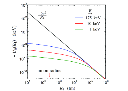
Figure 18: Folding potentials $U_{il}(R_{4})$ used to determine the Coulomb wave function $f_{ilLM}({\widetilde{K}}_{i},{\bf R}_{4})$ with the muon energy ${\widetilde{E}}_{i}$. The green, red, and blue curves illustrate $U_{il}(R_{4})$ for the cases of $l=2$ and $i=$ 16, 49, and 200, which correspond to the muon energies ${\widetilde{E}}_{i}\simeq$ 1, 10, and 175 keV, respectively. The black line denotes the pure Coulomb potential $-2e^{2}/R_{4}$.

Figure 18 illustrates the folding potentials for the muon energies $E_{i}=$ 1, 10, and 175 keV ($i=$ 16, 49, and 200, respectively); note that 1 keV almost corresponds to the the peak energy of the muon spectrum Fig. 15) and 10 keV is almost the mean energy of the emitted muon. The potentials asymptotically converge to the pure Coulomb potential $-2e^{2}/R_{4}$, but we note that they are very shallow in the region of muon amplitude $\psi_{0}^{({\rm N})}(R_{3,4})$ ($R_{4}\lesssim 10^{3}$ fm) of the total wave function $\Psi_{\frac{3}{2}M}^{(+)}(E)$ which appears as the ket wave function in the third member of the $T$-matrix (96).

If the discretization is made more precise by using larger $N$ values, the attractive folding potentials become shallower. Therefore, in actual calculations in Secs. VI A and B, we can neglect $U_{il}(R_{4})$ and replace $f_{ilLM}({\widetilde{K}}_{i},{\bf R}_{4})$ by the plane wave $e^{i{\widetilde{\bf K}}_{i}\cdot{\bf R}_{4}}$.

References

- (1)
- Frank (1947) F. C. Frank, Nature 160, 525 (1947).
- (3) A.D. Sakharov, Rep. Lebedev Phys. Inst. Acad. Sci. USSR (1948)
- (4) W.H. Breunlich, P. Kammel, J.S. Cohen, and M. Leon, Ann. Rev. Nucl. Part. Sci. 39, 311 (1989).
- (5) L.I. Ponomarev, Contemp. Phys. 31, 219 (1990).
- (6) P. Froelich, Adv. Phys., 41, 405 (1992).
- (7) K. Nagamine and M. Kamimura, Adv. Nucl. Phys. 24, 150 (1998).
- (8) K. Ishida et al., Hyperfine Interactions 138, 225 (2001).
- (9) N. Kawamura et al., Phys. Rev. Lett. 90, 043401 (2003).
- (10) S. E. Jones, Nature 321, 127 (1986).
- Iiyoshi et al. (2019) A. Iiyoshi, Y. Kino, M. Sato, Y. Tanahashi, N. Yamamoto, S. Nakatani, T. Yamashita, M. Tendler, and O. Motojima, AIP Conference Proceedings 2179, 020010 (2019).
- Yamashita et al. (submitted) T. Yamashita, K. Okutsu, Y. Kino, S. Okada, and M. Sato, Scientific Reports 12, 6393 (2022).
- Okada et al. (2020) S. Okada, et al., J. Low Temp. Phys. 200, 445 (2020).
- Paul et al. (2021) N. Paul, G. Bian, T. Azuma, S. Okada, and P. Indelicato, Phys. Rev. Lett. 126, 173001 (2021).
- Okumura et al. (2021) T. Okumura, et al., Phys. Rev. Lett. 127, 053001 (2021).
- Miyake et al. (2014) Y. Miyake, et al., J. Phys.: Conf. Ser. 551, 012061 (2014).
- (17) Y. Mori, Prog. Theor. Exp. Phys. 2021, 093G01 (2021).
- (18) N. Yamamoto, M. Sato, H. Takano, and A. Iiyoshi, Plasma Fusion Res. 16, 1405074 (2021).
- Rosen (1971) L. Rosen, Science 173, 490 (1971).
- Daniel (1984) H. Daniel, Nuclear Instruments and Methods in Physics Research Section B 3, 65 (1984).
- Kubo (2016) M. K. Kubo, Journal of the Physical Society of Japan 85, 091015 (2016).
- Nagamine (1989) K. Nagamine, Proceedings of the Japan Academy, Series B 65, 225 (1989).
- (23) K. Nagamine, Muon Catalyzed Fusion 5/6, 371,(1990/91).
- (24) K. Nagamine, Hyperfine Interact. 103, 123 (1996).
- Strasser et al. (1993) P. Strasser, K. Ishida, S. Sakamoto, M. Iwasaki, E. Torikai, K. Nagamine, and G. M. Marshall, Hyperfine Interact. 82, 543 (1993).
- (26) P. Strasser, K. Ishida, S. Sakamoto, K. Shimoura, N. Kawamura, E. Torikai, M. iwasaki, and K. Nagamine, Phys. Lett. B 368, 32 (1996).
- (27) H. Natori, PoSProc. Sci. 369 (NuFact2019), 090 (2020).
- Yamashita et al. (2021) T. Yamashita, K. Okutsu, Y. Kino, R. Nakashima, K. Miyashita, K. Yasuda, S. Okada, M. Sato, T. Oka, N. Kawamura, et al., Fus. Eng. Des. 169, 112580 (2021).
- Okutsu et al. (2021) K. Okutsu, T. Yamashita, Y. Kino, R. Nakashima, K. Miyashita, K. Yasuda, S. Okada, M. Sato, T. Oka, N. Kawamura, et al., Fus. Eng. Des. 170, 112712 (2021).
- (30) M. Kamimura, AIP Conference Proceedings 181 (1989) 330.
- (31) L.N. Bogdanova, V.E. Markushin, and V.S. Melezhik, Zh. Eksp. Teor. Fiz. 81, 829 (1981) [Sov. Phys. JETP 54, 442 (1981)].
- (32) L.N. Bogdanova, V.E. Markushin, V.S. Melezhik, L.I. Ponomarev, Sov. J. Nucl. Phys. 50, 848 (1989)
- (33) M.C. Struensee, G.M. Hale, R.T Pack, and J.S. Cohen Phys. Rev. A37, 340 (1988).
- (34) K. Szalewicz, B.Jeziorski, A. Scrinzi, X. Zhao, R. Moszynski, W. Kolos, P. Froelich, H. J. Monkhorst, and A. Velenik, Phys. Rev., A 42, 3768 (1990).
- (35) G.M. Hale, M.B. Chadwick, J.S. Cohen, and C.-Y. Hu, Hyperfine Interactions, 82, 213 (1993).
- (36) C.Y. Hu, G.M. Hale, and J.S. Cohen, Phys. Rev. A 49, 4481 (1994).
- (37) J.S. Cohen, G.M. Hale, and C.Y. Hu, Hyperfine Interactions, 101/102, 349 (1996).
- (38) B. Jeziorski, K. Szalewicz, A. Scrinzi, X. Zhao, R. Moszynski, W.Kolos, and A.Velenik, Phys. Rev., A 43, 1640 (1991).
- (39) P.D. Serpico, S. Esposito, F. Iocco, G.Mangano, G. Miele and O. Pisanti, J. Cosmol. Astropart. Phys. (JCAP) 0412, 010 (2004).
- (40) B. Haesner, W. Heeringa, H. O. Klages, H. Dobiasch, G. Schmalz, P. Schwarz, J. Wilczynski, B. Zeitnitz, and F. Käppeler, Phys. Rev. C 28, 995 (1983).
- (41) B. A. Lippmann and J. Schwinger, Phys. Rev. 79, 469 (1950).
- (42) M. Kamimura, Prog. Theor. Phys. Suppl. 62 (1977) 236.
- (43) M. Kamimura, Phys. Rev. A38, 621 (1988).
- (44) H. Kameyama, M. Kamimura and Y. Fukushima, Phys. Rev. C 40, 974 (1989).
- (45) E. Hiyama, Y. Kino and M. Kamimura, Prog. Part. Nucl. Phys. 51, 223 (2003).
- (46) M. Kamimura, M. Yahiro, Y. Iseri, Y. Sakuragi, H. Kameyama, and M. Kawai, Prog. Theor. Phys. Suppl. 89, 1 (1986).
- (47) N. Austern, Y. Iseri, M. Kamimura, M. Kawai, G. Rawitscher, and M. Yahiro, Phys. Rep. 154, 125 (1987).
- (48) M. Yahiro, K. Ogata, T. Matsumoto and K. Minomo, Prog. Theor. Exp. Phys. 2012, 1A206 (2012).
- (49) M. Kawai, M. Kamimura and K. Takesako, Prog. Theor. Phys. Suppl. 89, 118 (1986).
- (50) Y. Kino and M. Kamimura, Hyperfine Interactions, 82, 45 (1993).
- (51) M. Kamimura, E. Hiyama, and Y. Kino, Prog. Theor. Phys. 121, 1059 (2009).
- (52) H. Kanada, T. Kaneko, S. Nagata, and M. Nomote, Prog. Theor. Phys. 61, 1327 (1979).
- (53) H. Furutani, H. Kana, T. Kaneko, S. Nagata, H. Nishioka, S. Okabe, S. Saito, T. Sakuda, and M. Seya, Prog. Theor. Phys. Suppl. No. 68, 193 (1980).
- (54) F.C. Barker, Phys. Rev. C 56, 2646 (1997).
- (55) G.M. Hale, R.E. Brown, and N. Jarmie. Phys. Rev. Lett. 59, 763 (1987).
- (56) L.N. Bogdanova, G.M. Hale, and V.E. Markushin, Phys. Rev. C 44, 1289 (1991).
- (57) E. Hiyama and T. Yamada, Prog. Part. Nucl. Phys. 63, 339 (2009).
- (58) E. Hiyama, Few-Body Systems 53, 189 (2012).
-
(59)
E. Hiyama and M. Kamimura, Frontiers of Physics
13,
132106 (2018). - (60) M. Gell-Mann and M.L. Goldberger, Phys. Rev. 91, 369 (1953).
- (61) C.D. Stodden, H.J. Monkhorst, K. Szalewicz, and T.G. Winter, Phys. Rev. A 41, 1281 (1990).
- (62) C. Petitjean et al., Muon Catalyzed Fusion 5/6, 261 (1990/1991).
- (63) C. Petitjean, Hyperfine Interactions 138, 191 (2001).
- (64) M.C. Struensee and J.S. Cohen, Phys. Rev. A 38, 44 (1988).
- (65) V.E. Markushin, Muon Catal. Fusion, 3, 395 (1988).
- (66) H.E. Rafelski, B. Müller, J. Rafelski, D. Trautmann, and R.D. Viollier, Prog. Part. Nucl. Phys. 22, 279, (1989).
- (67) B. Müller, H. E. Rafelski, and J. Rafelski Phys. Rev. A 40, 2839, (1989).