Symbolic Implementation of Extensions of the PyCosmo Boltzmann Solver

Abstract

PyCosmo is a Python-based framework for the fast computation of cosmological model predictions. One of its core features is the symbolic representation of the Einstein-Boltzmann system of equations. Efficient C/C++ code is generated from the SymPy symbolic expressions making use of the sympy2c package. This enables easy extensions of the equation system for the implementation of new cosmological models. We illustrate this with three extensions of the PyCosmo Boltzmann solver to include a dark energy component with a constant equation of state, massive neutrinos and a radiation streaming approximation. We describe the PyCosmo framework, highlighting new features, and the symbolic implementation of the new models. We compare the PyCosmo predictions for the $\Lambda$CDM model extensions with CLASS, both in terms of accuracy and computational speed. We find a good agreement, to better than $0.1\%$ when using high-precision settings and a comparable computational speed. Links to the Python Package Index (PyPI) page of the code release and to the PyCosmo Hub, an online platform where the package is installed, are available at: https://cosmology.ethz.ch/research/software-lab/PyCosmo.html.

1 Introduction

Our understanding of the Universe relies on the possibility to predict cosmological observables from theoretical principles. One of the key theoretical predictions is the evolution over time of the linear order perturbations of the constituents of the Universe, captured by the Einstein-Boltzmann equations (see, e.g., Ma & Bertschinger [1995], Dodelson [2003]). The system of ordinary differential equations, due to its complexity and the coupling of the fields, needs to be solved numerically (see, e.g.,  Nadkarni-Ghosh & Refregier [2017]). For this purpose, several codes have been developed since the release of the pivotal Boltzmann code COSMICS [Bertschinger, 1995], closely followed in time by CMBFAST [Seljak & Zaldarriaga, 1996], later ported to C++ with the name CMBEASY [Doran, 2005a]. The currently maintained Boltzmann solvers are CAMB [Lewis et al., 2000], CLASS [Lesgourgues, 2011a] and PyCosmo  [Refregier et al., 2018]. Both for CAMB and CLASS  several codes have been written to include extensions beyond $\Lambda$CDM, for example hi_class [Zumalacárregui et al., 2017] and EFTCAMB [Hu et al., 2014] for modified gravity theories, CLASS_EDE [Hill et al., 2020] for early dark energy and CLASSgal [Dio et al., 2013] to include general relativistic effects in the computation of galaxy number counts. PyCosmo was introduced by Refregier et al. [2018] as a novel Python library that uses symbolic representation of equations for generating efficient C/C++ code. The framework includes both a Boltzmann solver as well as prediction tools for the computation of cosmological observables with several different fitting functions and approximations [Tarsitano et al., 2021]. With these tools, PyCosmo offers similar utilities as, e.g., the Core Cosmology Library CCL [Chisari et al., 2019] developed by the Dark Energy Science Collaboration (DESC).

An important feature of PyCosmo is the possibility to easily implement model extensions in symbolic form in the code, while taking advantage of the computational speed of the generated C/C++ code. This feature has been improved by rewriting and refactoring the related code as a new sympy2c package presented in Schmitt et al. [2022], which expands the idea of generating fast C/C++ code from symbolic representations of equations. Both sympy2c and PyCosmo are publicly available in the Python Package Index (PyPI). In this work, we illustrate how the PyCosmo Boltzmann solver can be extended thanks to the symbolic framework by implementing several extensions. We introduce two extensions of the Standard Model of Cosmology: a constant dark energy equation of state and massive neutrinos. We also include a radiation streaming approximation (RSA) for photons and massless relics, which approximates the evolution of radiation at late times and includes reionisation, following the treatment in Blas et al. [2011] implemented in CLASS. This approximation speeds up the code by reducing the number of equations in the ODE system and avoiding the reflection of power caused by the truncation of the multipole expansion of the radiation equations.

We begin by giving an overview of the new features of the PyCosmo framework in Section 2, where we discuss also the usage of the code and the precision settings used to compare with CLASS. We then present the equations of the models, implementation details and code comparisons with CLASS, both in terms of agreement and performance. In Section 3 we present the implementation of the constant dark energy equation of state, since it is a minimal modification of the Boltzmann system of equations for $\Lambda$CDM. We describe the inclusion of massive neutrinos, treated as non-interacting and non relativistic relics, in Section 4. In Section 5 we present the Radiation Streaming Approximation, which requires sympy2c to handle a switch between two different equation systems and is then applied to all models. In Section 6 we discuss the results obtained by benchmarking the speed of the computations and comparing the numerical results to CLASS. We conclude in Section 7. This work heavily relies on the Boltzmann equations presented in Ma & Bertschinger [1995]. To translate the PyCosmo notation to the Ma-Bertschinger and CLASS notation, we refer the reader to Appendix A. Appendix B presents the Einstein-Boltzmann system of ODE in PyCosmo notation, using $\ln{a}$ as the independent variable. The adiabatic initial conditions for $\Lambda$CDM and all the other implemented models are shown in Appendix C. We report in Appendix D the parameters of PyCosmo and CLASS that have been kept constant throughout the paper. In Appendix E, we provide a self contained summary of the computation of the total matter power spectrum, including general relativistic corrections, and using the $\mathcal{A}_{s}$ normalisation parameter.

2 PyCosmo framework

2.1 C/C++ code generation

We reimplemented and improved the C/C++ code generation related parts of previous versions of PyCosmo [Refregier et al., 2018] as a separate Python package named sympy2c which we describe in detail in Schmitt et al. [2022]. sympy2c translates symbolic representations of expressions and ordinary differential equations to C/C++ code and compiles this code as a Python extension module.

sympy2c replaces the Backward-Differentiation-Formula (BDF) solver from the previous version of PyCosmo by the established and robust Livermore Solver for Ordinary Differential Equations (LSODA) solver [Petzold, 1983] for improved step-size control and error diagnostics. LSODA detects stiff and nonstiff time domains automatically and switches between the nonstiff Adams method and the stiff BDF method. The BDF method solves a linear system derived from the Jacobian matrix of the differential equations at each time step. This affects runtime significantly for large systems. sympy2c leverages the symbolic form of the ODE and generates code to solve such systems efficiently by avoiding unnecessary computations based on the known sparsity structure of the involved Jacobian matrix.

To solve such linear systems sympy2c unrolls loops occurring in used LU factorization with partial pivoting (LUP) algorithm during code generation. This procedure depends on predetermined row permutations of the system, and the generated code includes checks for whether the considered permutation is appropriate for ensuring numerical accuracy. When solving the ODE, a new, not yet considered, permutation might arise. In this case, the solver delegates to a fall-back general LUP solver and records the new permutation. The result is a valid result but with a sub-optimal computation time. In this case, the warning message "there are new permutations pending, you might want to recompile" will be displayed together with the command necessary to recompile. Running the code-generator again will then also create optimized code for the newly recorded permutation(s), so that future runs of the solver will benefit from this. This approach starts with the identity permutation and could require several steps of solving the Boltzmann equations followed by code generation and compilation to achieve optimal performance. In our experiments not more than one such iteration is needed.

A large ODE systems can result in C/C++ functions with millions of lines of code which challenge the compiler and can cause long compilation times and high memory consumption, especially during the optimization phase of the compiler. To mitigate this, sympy2c can split the original matrix into smaller blocks and then generate code to implement blocked Gaussian elimination using Schur-complements. This affects the generated C/C++ code by creating more but significantly shorter functions and thus supports the optimization step of the compiler. Another benefit of this approach is that runtime is improved by reducing the number of cache misses on the CPU.

Depending on the size and sparsity structure of the system, this code generation and compilation step can take seconds up to 30 minutes or even more. PyCosmo and sympy2c  use caching strategies that consider previously generated code so that cached solvers are available within fractions of a second.

2.2 Usage

The equations for $\Lambda$CDM and the extended models are implemented symbolically in PyCosmo, both with and without radiation streaming approximation, in the CosmologyCore_model.py and CosmologyCore_model_rsa.py files. Supported models are currently "lcdm", "wcdm" or "mnulcdm".

The method PyCosmo.build initializes an instance of the Cosmo class for subsequent computations. Cosmo is the class that manages most of the functionalities of PyCosmo and on which all the other classes rely. PyCosmo.build requires the name of the model as well as all parameters which influence the code generation and compilation step. The argument rsa enables or disables the RSA and l_max specifies the maximum moment for truncating the photons and massless neutrinos hierarchies. The "mnulcdm" model also accepts parameters l_max_mnu and mnu_relerr which we describe later. Furthermore, parameters controlling the compiler, such as the optimization flag -On and the splits to use to reduce memory consumption and compilation time, can be specified when calling PyCosmo.build. All the parameters that can be passed to build are specified in Table 1.

Parameters which do not affect code generation, such as cosmological parameters, precision settings, parameters specific for approximations and physical constants can be set or modified using the Cosmo.set method. Each cosmological model is equipped with a default set of such parameters, contained in a default_model.ini file. Listing 1 demonstrates how to create a cosmology and change parameters.

⬇

1import PyCosmo

2cosmo = PyCosmo.build("lcdm", l_max=50, rsa=True)

3cosmo.set(omega_m=0.28)

4cosmo.print_params()

Listing 1: Creation of a $\Lambda$CDM cosmology using RSA and truncating photons and massless neutrino hierarchies at l_max = 50. We override the default value of $\Omega_{m}$ by $0.28$ and print a report of all parameter values.

One parameter that is particularly relevant is pk_type, since it allows the user to switch between the Boltzmann solver (pk_type = "boltz") and the approximations (pk_type = "EH" for the fitting function by Eisenstein and Hu [Eisenstein & Hu, 1998] and pk_type = "BBKS" for the BBKS polynomial fitting function [Peacock, 1997]). In this work we will always set pk_type = "boltz". Other cosmological and precision parameters which are kept fixed throughout the paper are reported in D. Tutorials for the computation of cosmological observables and the usage of the Boltzmann solver can be found on the PyCosmo Hub (see Tarsitano et al. [2021]), a public platform hosting the current version of PyCosmo, along with CLASS, CCL, and iCosmo [Refregier et al., 2011], an IDL predecessor of PyCosmo. The link to the PyCosmo Hub can be found at https://cosmology.ethz.ch/research/software-lab/PyCosmo.html.

2.3 Code comparisons setup

In order to validate the newly introduced models, we carry out detailed comparisons with CLASS. We evaluate the accuracy in terms of relative difference:

$$\mathrm{Relative\ difference({\texttt{PyCosmo}},{\texttt{CLASS}})}=\frac{X_{{\texttt{PyCosmo}}}-X_{{\texttt{CLASS}}}}{X_{{\texttt{PyCosmo}}}}$$

where $X$ is the cosmological observable we want to compare, for example the total matter power spectrum. Since this is a function of the wavenumber $k$, we compare it visually by plotting as a function of $k$ or, when specified, we look at the maximum relative difference in a $k$ interval.

Comparing the two codes implies carefully setting the cosmological parameters and the precision settings. In the case of CLASS, we use the precision files shipped with the code: cl_permille.pre for fast and accurate computation and pk_ref.pre for high precision. cl_permille.pre guarantees a precision of $0.1\%$ up to $k=1h\mathrm{Mpc^{-1}}$ for the matter power spectrum, and pk_ref.pre a precision of $0.001\%$ on scales $k<50h\mathrm{Mpc^{-1}}$ [Lesgourgues, 2011b]. Both CLASS precision settings use the Radiation Streaming Approximation, described in detail in Section 5. They also include the Tight Coupling Approximation and Ultra-relativistic Fluid Approximation (see Blas et al. [2011]), whereas only cl_permille.pre uses the fluid approximation for massive neutrinos (presented in Lesgourgues & Tram [2011]). The main parameters controlling precision in PyCosmo are the l_max parameter which defines the truncation of the multipole hierarchy for radiation fields (same for photons and massless neutrinos) and the boltzmann_rtol and boltzmann_atol parameters defining the relative and absolute tolerance of the LSODA ODE solver. Massive neutrinos also add two important precision parameters which will be described more in detail in section 4: mnu_relerr controlling the number of momenta $q$ used for the massive neutrino integrals and l_max_mnu, controlling the truncation of the multipole expansion for massive neutrinos. We summarise all the precision parameters available in PyCosmo in Table 1.

Parameter	Description	Method	Deafult
rsa	Switch for the RSA	build	False
compilation_flags	GCC compiler’s optimization flag	build	“-O3”
splits	Splittings of the ODE system	build	None
reorder	Whether to reorder the ODE system to speed up	build	True
	code generation when using splits
l_max	Hierarchy truncation of the relativistic relics	build	20
l_max_mnu	Hierarchy truncation of massive neutrinos	build	20
mnu_relerr	Relative error for massive neutrinos integral	build	1e-5
sec_factor	Safety factor for permuting rows	set	10
	in the LUP decomposition within LSODA
boltzmann_rtol	Relative tolerance of the LSODA solver	set	1e-5
boltzmann_atol	Absolute tolerance of the LSODA solver	set	1e-5
boltzmann_max_bdf_order	Maximum order used by the BDF integrator	set	5
boltzmann_max_iter	Max number of iterations of the LSODA solver	set	2000000

Table 1: Description of the precision parameters available in the PyCosmo Boltzmann solver, along with the method they are passed to and their default values.

The two precision settings that we use in PyCosmo when comparing respectively to CLASS cl_permille.pre and pk_ref.pre are:

• speed: l_max = $17$, l_max_mnu = $17$, rtol = $10^{-5}$, atol = $10^{-5}$, mnu_relerr = $10^{-5}$

• precision: l_max = $50$, l_max_mnu = $50$, rtol = $10^{-6}$ and atol =$10^{-6}$, mnu_relerr = $10^{-6}$.

When using the RSA in PyCosmo, we set the RSA trigger parameters (detailed in Section 5) to:

• speed: rsa_trigger_taudot_eta = 5, rsa_trigger_k_eta = 45

• precision: rsa_trigger_taudot_eta = 100, rsa_trigger_k_eta = 240

which match the equivalent CLASS parameters in cl_permille.pre and pk_ref.pre. All the other precision parameters have default values, as in Table 1. We do not attempt to exactly match the precision parameters in the two packages, since CLASS includes a number of approximations that are not available in PyCosmo. It is possible to switch off most of the approximations but this would imply losing the precision guarantees of the default precision files.

The cosmological parameters that remain constant throughout the paper are listed in Appendix D, whereas the matter energy density $\Omega_{m}$, the number of massless neutrinos $N_{\nu}$, the number of massive neutrinos $N_{\nu,m}$, the total sum of the massive neutrinos $\Sigma m_{\nu}$ and the dark energy equation of state parameter $w_{\mathrm{de}}$ (corresponding in CLASS to $\Omega_{cdm}=\Omega_{m}-\Omega_{b}$ since $\Omega_{b}$ is fixed, $N_{ur}$, $N_{ncdm}$, $m_{ncdm}$ = $\Sigma m_{\nu}/N_{\nu,m}$ and $w_{0,fld}$) change in different models and are reported in the corresponding sections. $\Omega_{\Lambda}$ is computed by imposing the flatness condition $\sum_{i}\Omega_{i}=1$.

3 A simple model: Dark Energy with a constant equation of state

3.1 Equations

In order to search for deviations from a cosmological constant, we consider here a dark energy equation of state with $w_{\mathrm{de}}=p_{\mathrm{de}}/\rho_{\mathrm{de}}\neq-1$. The equations for this model have been studied in detail in Ballesteros & Lesgourgues [2010], and experimental constraints have been presented in, e.g., Tripathi et al. [2017], Scolnic et al. [2018], Aghanim et al. [2020], Abbott et al. [2021].

For a constant dark energy equation of state $w_{\mathrm{de}}$, the dark energy density is given by

$$\rho(a)=\rho_{0}\cdot a^{-3(1+w_{\mathrm{de}})}.$$ (1)

We immediately see that $\rho=\textrm{const}$. for a cosmological constant with $w_{\mathrm{de}}=-1$. The Hubble parameter is given by

$$\frac{H(a)}{H_{0}}=\Big{[}\Omega_{r}a^{-4}+\Omega_{m}a^{-3}+\Omega_{\kappa}a^{-2}+\Omega_{\Lambda}\cdot a^{-3(1+w_{\mathrm{de}})}\Big{]}^{\frac{1}{2}}.$$ (2)

In this equation, $\Omega_{r}$ is the radiation density which includes photons and massless neutrinos, $\Omega_{m}$ the matter density, $\Omega_{\kappa}$ the curvature density (listed for completeness, even though the Boltzmann solver in PyCosmo currently only supports flat models) and $\Omega_{\Lambda}$ the dark energy density. In all cases, $\Omega_{i}$ is defined as the fraction of the energy density of the corresponding component today and the critical energy density $\rho_{\mathrm{crit}}$ of the Universe.

In the case of a cosmological constant, there are no dark energy perturbations. For $w_{\mathrm{de}}\neq-1$, we can write down the dark energy equations following Ma & Bertschinger [1995], Dodelson [2003] and obtain

$$\begin{split}\dot{\delta}_{\mathrm{de}}&=-(1+w_{\mathrm{de}})(ku_{\mathrm{de}}+3\dot{\Phi})-3\frac{\dot{a}}{a}\Big{(}\frac{\delta p_{\mathrm{de}}}{\delta\rho_{\mathrm{de}}}-w_{\mathrm{de}}\Big{)}\delta_{\mathrm{de}}\\ \dot{u}_{\mathrm{de}}&=-\frac{\dot{a}}{a}\Big{(}1-3w_{\mathrm{de}}\Big{)}u_{\mathrm{de}}+\frac{\delta p_{\mathrm{de}}/\delta\rho_{\mathrm{de}}}{1+w_{\mathrm{de}}}k\delta_{\mathrm{de}}-k\sigma_{\mathrm{de}}+k\Psi,\end{split}$$ (3)

where all derivatives are with respect to the conformal time $\eta$ and we use the conformal Newtonian gauge as in Refregier et al. [2018]. The anisotropic stress, $\sigma_{\mathrm{de}}$, vanishes, which deletes one term in the second perturbation equation.

In general, the sound speed $\tilde{c}_{\mathrm{s,de}}^{2}=\frac{\delta p_{\mathrm{de}}}{\delta\rho_{\mathrm{de}}}$ is a Gauge-dependent variable, which can be expressed in terms of the rest frame sound speed $c_{\mathrm{s,de}}^{2}$ and the adiabatic sound speed $c_{\mathrm{a}}^{2}$. The latter is equal to $w_{\mathrm{de}}$ for a constant dark energy equation of state [Ballesteros & Lesgourgues, 2010]. Here, we use the expression [Ballesteros & Lesgourgues, 2010]

$$\tilde{c}_{\mathrm{s,de}}^{2}\delta_{\mathrm{de}}=c_{\mathrm{s,de}}^{2}\delta_{\mathrm{de}}+3\frac{d\ln{a}}{d\eta}(1+w_{\mathrm{de}})(c_{\mathrm{s,de}}^{2}-w_{\mathrm{de}})\frac{u_{\mathrm{de}}}{k},$$ (4)

which is valid for a constant dark energy equation of state.

Inserting this expression in Eq. 3 we obtain

$$\begin{split}\dot{\delta}_{\mathrm{de}}&=-(1+w_{\mathrm{de}})(ku_{\mathrm{de}}+3\dot{\Phi})-3\frac{\dot{a}}{a}\Big{(}c_{\mathrm{s,de}}^{2}-w_{\mathrm{de}}\Big{)}\delta_{\mathrm{de}}-9\Big{(}\frac{\dot{a}}{a}\Big{)}^{2}(1+w_{\mathrm{de}})(c_{\mathrm{s,de}}^{2}-w_{\mathrm{de}})\frac{u_{\mathrm{de}}}{k}\\ \dot{u}_{\mathrm{de}}&=-\frac{\dot{a}}{a}(1-3c_{\mathrm{s,de}}^{2})u_{\mathrm{de}}+\frac{c_{\mathrm{s,de}}^{2}}{1+w_{\mathrm{de}}}k\delta_{\mathrm{de}}+k\Psi.\end{split}$$ (5)

Compared to the system of equations in Refregier et al. [2018], the Einstein equations are modified to

$$k^{2}\Phi+3\frac{\dot{a}}{a}\left(\dot{\Phi}-\frac{\dot{a}}{a}\Psi\right) = 4\pi Ga^{2}\left[\rho_{m}\delta_{m}+4\rho_{r}\Theta_{r0}+\rho_{\mathrm{de}}\delta_{\mathrm{de}}\right]$$ (6)

$$\dot{\Phi}-\frac{\dot{a}}{a}\Psi = -4\pi G\frac{a^{2}}{k}\left[\rho_{m}u_{m}+4\rho_{r}\Theta_{r1}+\rho_{\mathrm{de}}(1+w_{\mathrm{de}})u_{\mathrm{de}}\right]$$ (7)

$$k^{2}(\Phi+\Psi) = -32\pi Ga^{2}\rho_{r}\Theta_{r2}.$$ (8)

In order to evolve the perturbation equations, we also need to define the initial conditions for these. We choose the adiabatic initial conditions from CLASS, outlined in Ballesteros & Lesgourgues [2010] in the synchronous gauge, and then transform them into the conformal Newtonian gauge. We report the initial conditions for all the fields in Appendix C.

3.2 Numerical implementation

In order to implement the new equations outlined in the previous section, we generated a new file for the symbolic Boltzmann equations, called CosmologyCore_wcdm.py. This can be used instead of the default equations file CosmologyCore.py for the $\Lambda$CDM model, by setting the model to "wcdm" as shown in Listing 1.

In PyCosmo, all derivatives are written with respect to $\ln{a}$ (in the code lna) instead of $\eta$. The perturbation equations for a $\Lambda$CDM model in this notation are detailed in B. In the previous section, we presented the dark energy perturbation equations with respect to $\eta$. Using the conversion $\frac{d\ln{a}}{d\eta}=aH$, we can rewrite the two dark energy perturbation equations from Eq. 5 as

$$\begin{split}\frac{d\delta_{\mathrm{de}}}{d\ln{a}}&=-(1+w_{\mathrm{de}})\Big{(}\frac{ku_{\mathrm{de}}}{aH(a)}+3\frac{d\Phi}{d\ln{a}}\Big{)}-3(c_{\mathrm{s,de}}^{2}-w_{\mathrm{de}})\Big{(}\delta_{\mathrm{de}}+3(1+w_{\mathrm{de}})\frac{aH(a)u_{\mathrm{de}}}{k}\Big{)}\\ \frac{du_{\mathrm{de}}}{d\ln{a}}&=-(1-3c_{\mathrm{s,de}}^{2})u_{\mathrm{de}}+\frac{c_{\mathrm{s,de}}^{2}}{1+w_{\mathrm{de}}}\frac{k\delta_{\mathrm{de}}}{aH(a)}+\frac{k}{aH(a)}\Psi.\end{split}$$ (9)

Then the two dark energy perturbation equations in Eq. 9 can be expressed with SymPy as

⬇

1ddelta_de_dlan = - (1 + w0) * (k / (a * H) * u_de + 3 * dPhi_dlan)

2 - 3 * (cs_de2 - w0) * delta_de

3 - 9 * (1 + w0) * (cs_de2 - w0) * (a * H) / k * u_de

4

5du_de_dlan = - (1 - 3 * cs_de2) * u_de

6 + cs_de2 / (1 + w0) * k * delta_de / (a * H)

7 + k / (a * H) * Psi

Listing 2: The two dark energy perturbation equations as implemented in CosmologyCore_wcdm.py.

CosmologyCore_wcdm.py also contains the background equations and the initial conditions for the linear perturbations.

3.3 Code comparisons

In Figure 1 we show the dark energy perturbations $\delta_{\mathrm{de}}$ and $u_{\mathrm{de}}$ as a function of scale factor $a$ for three wavenumbers $k=0.005,0.05$ and $5\ \mathrm{Mpc}^{-1}$, plotted both with PyCosmo as well as CLASS. We also display the relative difference between the evolution of the perturbations obtained by the two codes. The cosmology we consider is

• $w$CDM: {$\Omega_{\Lambda}$, $\Omega_{m}$, $N_{\nu}$, $N_{\nu,m}$, $\Sigma m_{\nu}$, $w_{\mathrm{de}}$} = {0.69992, 0.3, 3.044, 0, 0, -0.9}

with all other parameters as specified in D and using the precision settings from 2.3. In general, we find good agreement between the codes. When the fields are highly oscillating around zero, we observe a degradation of the agreement, as expected, given the impact of step-size control and numerical precision of the solver in that regime. We also notice a discrepancy at initial time for small values of $k$, which is caused by the tight coupling approximation in CLASS. In Figure 2 we show the wCDM total matter power spectrum computed with the two codes for 200 log-spaced $k$ values between $10^{-4}$ and $10\ \mathrm{Mpc^{-1}}$ at redshifts $z=0$, $z=1$ and $z=5$. In general, we observe that the results for $w$CDM show the same level of agreement with CLASS as $\Lambda$CDM. The discrepancies tend to grow on large scales for $z=5$ but remain below the $10^{-3}$ level. The same is observed for higher redshifts. In Section 6 we summarize the comparisons in terms of computing time and power spectrum relative difference for different $k$ ranges at $z=0$.

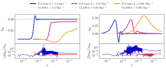
Figure 1: In the top left panel, we show the dark energy perturbation $\delta_{\mathrm{de}}$ as a function of scale factor $a$ for a dark energy equation of state with $w=-0.9$ and sound speed $c_{\mathrm{s,de}}^{2}=1$ at three values of the wavenumber $k=0.005,0.05$ and $5\ \mathrm{Mpc}^{-1}$. In the top right panel, we show dark energy perturbation $u_{\mathrm{de}}$ as a function of scale factor $a$ for the same wavenumbers. Perturbations computed with PyCosmo are displayed by thick lines, while CLASS values by dash-dotted lines. The bottom panels display relative differences between the two codes.

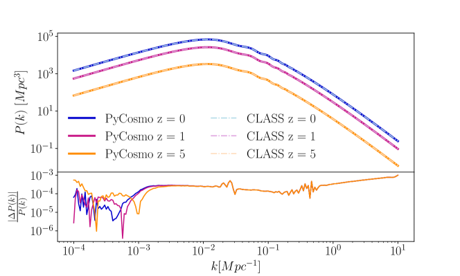
Figure 2: Total matter power spectrum at redshifts $z=0$, $z=1$ and $z=5$ for a dark energy equation of state with $w=-0.9$ and sound speed $c_{\mathrm{s,de}}^{2}=1$, plotted both with PyCosmo (thick solid lines) and CLASS (dash-dotted lines) for 200 log-spaced $k$ values between $10^{-4}$ and $10\ \mathrm{Mpc^{-1}}$. On the bottom panel we display the relative difference between the two codes.

4 A complex model: Massive Neutrinos

4.1 Equations

Oscillation experiments provide evidence that neutrinos have mass (see e.g. Fukuda et al. [1998], Ahmad et al. [2002], Eguchi et al. [2003] and also de Salas et al. [2021] for a recent global fit of neutrino oscillation data) and since their masses are imprinted onto cosmological observables, we need to include the evolution of light massive relics in the system of equations. This allows cosmological probes to constrain the properties of neutrinos, in particular the sum of the neutrino masses (see e.g. Lesgourgues & Pastor [2006], Lesgourgues et al. [2013], Lattanzi & Gerbino [2018] for reviews on neutrino cosmology).

In this section, we present the implementation of the Einstein-Boltzmann equations for massive neutrinos into the PyCosmo Boltzmann solver. Massive neutrinos modify both the background evolution and the linear order perturbations. Qualitatively, massive neutrinos undergo a phase transition: they behave like radiation at early times, when they are fully relativistic, and shift to a matter-like behaviour at late times (see, e.g., Lattanzi & Gerbino [2018], Ichikawa et al. [2005]). The transition happens smoothly through cosmic time and the dependence on mass, scale factor and momentum in the evolution of the distribution function prevents from integrating out the momentum dependence. This can be done only when considering approximations. For this reason, the inclusion of massive neutrinos in the Boltzmann equations is highly non trivial and has a strong impact on the size of the ODE system.

In this section we write the equations for $N_{\nu,m}$ massive neutrinos with degenerate masses and total neutrino mass sum $\Sigma m_{\nu}$, where the sum goes over the three neutrino mass eigenstates. A generalization to neutrinos with different masses is simply achieved by suppressing the $N_{\nu,m}$ in front of the equations and writing separate equations for each neutrino species with mass $m_{\nu,i}$. In PyCosmo we introduce degenerate massive neutrinos. The introduction of neutrino hierarchies is left as future development.

The massive neutrino density can be written as

$$\rho_{\nu,m}(a)=4\pi a^{-4}\int_{0}^{\infty}dqq^{2}f_{0}(q)\epsilon,$$ (10)

where $q=ap$, with $p$ the proper momentum, related to the 4-momentum by $P_{i}=a(1-\Phi)p_{i}$ in the Newtonian conformal gauge. Then $\epsilon=\sqrt{q^{2}+a^{2}m^{2}}$ is the proper energy measured by a comoving observer multiplied by the scale factor and $f_{0}(q)$ is the Fermi-Dirac distribution

$$f_{0}(q)=\frac{g_{s}}{(2\pi\hbar)^{3}}\frac{1}{e^{q/k_{b}T_{0}}+1},$$ (11)

where $g_{s}$ is the spin degeneracy factor that equals $2N_{\nu,m}$ in the case of degenerate neutrinos. $T_{0}$ is the temperature of the Cosmic Neutrino Background today expressed in units of the CMB temperature $T_{0}=T_{{\nu},m}T_{\mathrm{CMB}}$, $T_{{\nu},m}=\left(\frac{4}{11}\right)^{1/3}$ for neutrinos that undergo instantaneous decoupling and $k_{b}$ is the Boltzmann constant. The Friedmann equation results in

$$\frac{H(a)}{H_{0}}=\left[(\Omega_{r}+\Omega_{\nu,m}(a))a^{-4}+\Omega_{m}a^{-3}+\Omega_{\kappa}a^{-2}+\Omega_{\Lambda}\right]^{\frac{1}{2}}$$ (12)

where $\Omega_{r}$ still includes massless neutrinos if present (denoted with the subscript $\nu$ such that $\Omega_{r}=\Omega_{\gamma}+\Omega_{\nu}$), whereas the massive neutrino energy density is $\Omega_{\nu,m}(a)$. Note that we factor out the $a^{-4}$ term from $\Omega_{\nu,m}(a)$ for similarity with the other energy densities, but $\Omega_{\nu,m}(a)$ still contains a dependency on the scale factor $a$, differently from the other species, since the proper energy $\epsilon$ contains a factor of $a$ that we cannot integrate out (see equation 10, $\Omega_{\nu,m}(a)a^{-4}=\rho_{\nu,m}(a)/\rho_{crit}$).

The massive neutrino perturbations arise from a linear expansion of the distribution function $f(x,q,\hat{q},\eta)=f_{0}(q)\left[1+\mathcal{M}(x,q,\hat{q},\eta)\right]$ around the Fermi-Dirac distribution $f_{0}(q)$. The function $\mathcal{M}(x,q,\hat{q},\eta)$ is Fourier transformed and expanded in a Legendre series as

$$\mathcal{M}(\vec{k},\hat{q},q,\eta)=\sum_{l=0}^{\infty}(-i)^{l}(2l+1)\mathcal{M}_{l}(\vec{k},q,\eta)P_{l}(\mu)$$ (13)

with $\mu=\hat{k}\cdot\hat{q}$, $\mathcal{P}_{l}$ the Legendre polynomials and $\mathcal{M}_{l}$ defined as

$$\mathcal{M}_{l}=\frac{1}{(-i)^{l}}\int_{-1}^{1}\frac{d\mu}{2}{\mathcal{P}}_{l}(\mu)\mathcal{M}(\mu).$$ (14)

The massive neutrino Boltzmann equations are then derived similarly to those of the ultra-relativistic fields, setting the collision term to $0$, since neutrinos are only weakly interacting. Using the definition of $\mathcal{M}_{l}$ to express the Boltzmann equations as a hierarchy of moments, we obtain

$$\dot{\mathcal{M}}_{0} =-\frac{qk}{\epsilon}\mathcal{M}_{1}-\dot{\Phi}\frac{d\ln{f_{0}}}{d\ln q}$$ (15)

$$\dot{\mathcal{M}}_{1} =\frac{qk}{3\epsilon}\left(\mathcal{M}_{0}-2\mathcal{M}_{2}\right)-\ \frac{\epsilon k}{3q}\Psi\frac{d\ln{f_{0}}}{d\ln{q}}$$ (16)

$$\dot{\mathcal{M}}_{l} =\frac{qk}{(2l+1)\epsilon}\left[l\mathcal{M}_{l-1}-(l+1)\mathcal{M}_{l+1}\right],\ \ l\geq 2.$$ (17)

The hierarchy is truncated at a multipole $l_{max}$ (l_max_mnu in the code) when solving the system of equations numerically with a hierarchy truncation from Ma & Bertschinger [1995], which is analogous to that for photons and massless neutrinos

$$\dot{\mathcal{M}}_{l_{max}}\simeq\frac{qk}{\epsilon}\mathcal{M}_{l_{max}-1}-\frac{(l_{max}+1)}{\eta}\mathcal{M}_{l_{max}}.$$ (18)

Massive neutrinos also modify the Einstein equations due to the extra terms in the stress-energy tensor. These now read

$$k^{2}(\Psi+\Phi) =-12\left(\frac{H_{0}}{a}\right)^{2}\left(\Omega_{\gamma}\Theta_{2}+\Omega_{\nu}\mathcal{N}_{2}+\frac{N_{\nu,m}}{(2\pi)^{2}\rho_{crit}}\int{q^{2}dq\frac{q^{2}}{\epsilon}\frac{\mathcal{M}_{2}}{e^{q/k_{b}T_{0}}+1}}\right)$$ (19)

$$k^{2}\Phi+3\frac{\dot{a}}{a}\left(\dot{\Phi}-\frac{\dot{a}}{a}\Psi\right) =\frac{3}{2}\left(H_{0}a\right)^{2}\left[\Omega_{m}\delta_{m}a^{-3}+4a^{-4}\left(\Omega_{r}\Theta_{r0}+\frac{N_{\nu,m}}{(2\pi)^{2}\rho_{crit}}\int{q^{2}dq\frac{\epsilon\mathcal{M}_{0}}{e^{q/k_{b}T_{0}}+1}}\right)\right],$$

where $\Omega_{m}\delta_{m}$ is a shortcut for $\Omega_{dm}\delta+\Omega_{b}\delta_{b}$, $\Omega_{r}\Theta_{r0}=\Omega_{\gamma}\Theta_{0}+\Omega_{\nu}\mathcal{N}_{0}$ and $\rho_{crit}$ is the critical energy density of the Universe. The massive neutrino quantities we are interested in are the density fluctuation, the fluid velocity and the shear stress which are computed by integrating over the moments $\mathcal{M}_{l}$:

$$\delta_{\nu,m} =\frac{\int{q^{2}dq\epsilon f_{0}(q)\mathcal{M}_{0}}}{\int{q^{2}dq\epsilon f_{0}(q)}}$$ (20)

$$u_{\nu,m} =\frac{\int{q^{2}dqqf_{0}(q)\mathcal{M}_{1}}}{\int{q^{2}dq\epsilon f_{0}(q)}+\frac{1}{3}\int{q^{2}dq\frac{q^{2}}{\epsilon}f_{0}(q)}}$$

$$\sigma_{\nu,m} =\frac{2}{3}\frac{\int{q^{2}dq\frac{q^{2}}{\epsilon}f_{0}(q)\mathcal{M}_{2}}}{\int{q^{2}dq\epsilon f_{0}(q)}+\frac{1}{3}\int{q^{2}dq\frac{q^{2}}{\epsilon}f_{0}(q)}}.$$

Note that in the PyCosmo implementation, we substitute $q$ with $q^{\prime}=\frac{q}{k_{b}T_{0}}$ for convenience.

4.2 Numerical implementation

The implementation of the massive neutrino equations uses sympy2c similarly to the PyCosmo implementation of $\Lambda$CDM and $w$CDM. The background integral over momentum $q$ is computed using indefinite numerical integration from sympy2c , whereas the integrals at perturbation level use a Gauss-Laguerre quadrature integration scheme in our symbolic representation of the ODE system, since we need to evolve a finite number of equations. This follows the approach used in Lesgourgues & Tram [2011]. The number of discrete $q$ values is governed by the parameter mnu_relerr, which sets the relative difference between the Gauss-Laguerre integration of a test function ($\sum_{n=2}^{n=4}q^{n}f_{0}(q)$) with respect to its analytical result. This parameter is specified using PyCosmo.build since it affects the size of the ODE system and thus also code generation. We introduce an additional parameter influencing code generation in addition to the truncation parameter l_max of the photon and massless neutrino hierarchies: l_max_mnu that truncates the Legendre series $\mathcal{M}_{l}$ as described above.

The implementation of massive neutrino cosmologies results in a large systems of equations and thus C functions with millions of lines of generated code, challenging the optimizer of the used C compiler. To mitigate significantly compilation time and memory requirements, we enable sympy2c to use the matrix splitting feature (enabled by specifying the splits parameter and reorder=True in PyCosmo.build) described in Section 2. The user can also pass a compilation_flags parameter, that enables or disables compiler optimizations of the C code and has a diametrical effect on compilation vs. runtime.

We implement initial conditions for massive neutrinos that match the adiabatic initial conditions in CLASS and Cosmics and can be triggered using the initial_conditions parameter. We report the equations in Appendix C.

4.3 Code comparisons

One of the key effects of massive neutrinos on cosmological observables is the suppression of small scale matter overdensities due to neutrino free streaming [Lesgourgues & Pastor, 2006]. In Figure 3 we show the total matter power spectrum obtained with PyCosmo and CLASS for 200 log-spaced $k$ values between $10^{-4}$ and $10\ \mathrm{Mpc^{-1}}$ at redshifts $z=0$, $z=1$ and $z=5$ with the following cosmological parameters:

• degenerate $\Sigma m_{\nu}$ = 60 meV: {$\Omega_{m}$, $N_{\nu}$, $N_{\nu,m}$, $\Sigma m_{\nu}$, $w_{\mathrm{de}}$} = {0.29869, 0.00440, 3, 0.06, -1}.

All other parameters are set to default values (see D) and we use the precision settings for the two codes (see 2.3). In the bottom panel we display the relative difference between PyCosmo and CLASS.

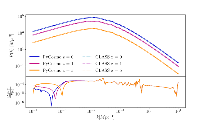
Figure 3: Total matter power spectrum at redshifts $z=0$, $z=1$ and $z=5$ for a cosmology with three massive neutrinos with $\Sigma m_{\nu}$ = 60 meV, plotted both with PyCosmo and CLASS for 200 log-spaced $k$ values between $10^{-4}$ and $10\ \mathrm{Mpc^{-1}}$. In the bottom panel, we display the relative difference between the two codes.

In Appendix E we outline the equation of the total matter power spectrum, following a fully general relativistic treatment in the presence of massive neutrinos [Yoo et al., 2009, Yoo, 2010, Bonvin & Durrer, 2011, Challinor & Lewis, 2011, Dio et al., 2013]. In general, we observe a very good agreement, with a maximum relative discrepancy of $5\times 10^{-4}$ on intermediate scales. The redshift evolution does not impact the agreement. We also show the suppression of the total matter power spectrum with respect to the power spectrum with massless neutrinos in Figure 4 both for $\Sigma m_{\nu}$ = 60 meV and 120 meV ($\Omega_{m}$=0.29737), when keeping $\Omega_{m,tot}=\Omega_{m}+\Omega_{\nu,m}$ fixed to $\Omega_{m,tot}=0.3$ and $N_{\mathrm{eff}}=3.044$. The cosmological parameters for the $\Lambda$CDM model are set to:

• $\Lambda$CDM: {$\Omega_{m}$, $N_{\nu}$, $N_{\nu,m}$, $\Sigma m_{\nu}$, $w_{\mathrm{de}}$} = {0.3, 3.044, 0, 0., -1}.

On the left panel of the figure, we show the suppression of the power spectrum computed with PyCosmo and CLASS, using the default precision settings and the relative difference between the two codes. The suppression has a large discrepancy at low $k$ values when it is approaching and crossing zero. Furthermore, there is a $\sim 1\%$ difference on small scales (large $k$ values), where the effects of the hierarchy truncation and the approximations are most dominant. We verify that this discrepancy is reduced when matching the l_max parameters in the two codes (l_max_g = l_max_pol_g = l_max_ur = l_max_ncdm = 50 in CLASS, PyCosmo remains in precision settings) and suppressing the Ultra-relativistic Fluid Approximation in CLASS, as shown in the right panel of Figure 4.

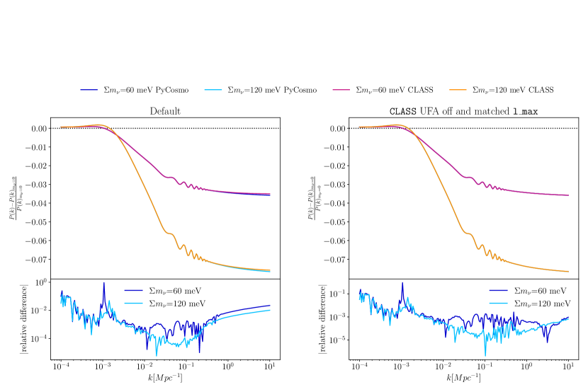
Figure 4: Suppression of the total matter power spectrum for two cosmologies with three neutrinos and $\Sigma m_{\nu}$ = 60 and 120 meV, respectively, compared to a $\Lambda$CDM cosmology with massless neutrinos only computed with PyCosmo and CLASS. For all cosmologies, we set the total matter density to $\Omega_{m,tot}$ = 0.3 and $N_{\mathrm{eff}}=3.044$. The left panel displays the power spectrum and the relative difference with the default precision settings for CLASS and PyCosmo. In the right plot, we display the same quantities when setting l_max = 50 for all the radiation fields and massive neutrinos and switching off the UFA in CLASS.

5 An approximation scheme: Radiation Streaming Approximation

5.1 Equations

After decoupling, photons and massless neutrinos behave approximately like test particles free-streaming in the gravitational field determined by the massive components, making it possible to derive a non-oscillatory solution of the inhomogeneous Boltzmann equations inside the Hubble radius. This approximation, called the Radiation Streaming Approximation (RSA), was introduced in the Newtonian gauge by Doran [2005b] and in the synchronous gauge by Blas et al. [2011]. This treatment allows both to avoid unphysical oscillations resulting from the hierarchy truncation and to speed up the integration, which is slowed down by fast late time oscillations of the radiation fields especially on small scales. At late times, the approximation does not need to be precise, since the contribution of the radiation energy density to the overall energy density is negligible. This approximation only impacts the linear perturbations. The evolution of the relativistic fields can be written as

$$\begin{split}\Theta_{0}&=\Phi+\frac{\dot{\tau}u_{b}}{k}\\ \Theta_{1}&=-\frac{2}{k}\dot{\Phi}+\frac{\dot{\tau}}{k}\left(\frac{aH}{k}u_{b}-c_{b}^{2}\delta_{b}+\Phi\right)\\ \mathcal{N}_{0}&=\Phi\\ \mathcal{N}_{1}&=-\frac{2}{k}\dot{\Phi}\\ \Theta_{2}&=\Theta_{P0,1,2}=\mathcal{N}_{2}=0,\\ \end{split}$$ (21)

with all the higher order multipoles set to 0. This approximation is switched on when two conditions are satisfied, following the CLASS [Blas et al., 2011] scheme:

• $\texttt{rsa\_trigger\_k\_eta}\leq k\eta$

• $\texttt{rsa\_trigger\_taudot\_eta}\leq-(\dot{\tau}\eta)^{-1}$,

corresponding to decoupled radiation within the horizon.

5.2 Numerical implementation

In order to implement the Radiation Streaming Approximation within PyCosmo  we use a functionality from sympy2c  to switch between two different ODEs at a dynamically computed time point.

This requires:

• Two ODE systems specified as sympy2c OdeFast objects. In our case these will be the symbolic representations of the model of interest ($\Lambda$CDM, $\Lambda$CDM with massive neutrinos or $w$CDM) and its equivalent RSA system. Note that the two systems can have different dimensions.

• A switch_time function which determines at which time to switch from the first system of equations to the second. In the RSA implementation we use the switching conditions described above.

• A switch function, computing the initial conditions for the second system of equations from the state of the first system before and at the switching time. In the RSA implementation, this function just discards the matrix entries for the fields $\Theta_{i}$, $\Theta_{Pi}$ and $\mathcal{N}_{i}$, $i\geq 0$ since $\Theta_{0}$, $\Theta_{1}$, $\mathcal{N}_{0}$ and $\mathcal{N}_{1}$ have analytical expressions and thus do not need initial conditions.

• A merge function which specifies how to combine the matrix valued results from both numerical solutions into a final matrix. Our RSA implementation keeps the full matrix from the solution of the full system of equations and extends the matrix from the RSA solution using the analytical formula for $\Theta_{i}$ and $\mathcal{N}_{i}$ for $i\leq 1$. All other entries are set to $0$ for $i\geq 2$ and for all the polarization terms $\Theta_{Pi}$.

In order to use the RSA in PyCosmo  one needs to pass the rsa = True flag to PyCosmo.build for any of the models. This will switch the CosmologyCore_model.py equation file to a
CosmologyCore_model_rsa.py file containing the RSA equations for the radiation fields and all the other equations of the system.

5.3 Internal code consistency

The main achievement obtained by implementing the RSA is a significant reduction of the computation time for the fields, especially for high values of $k$, as we will discuss in detail in the next section. This is especially true when choosing the $\Lambda$CDM and $w$CDM models, where most of the system of ODEs consists of radiation perturbations. In Figure 5, we show the effects of the RSA and of the hierarchy truncation on the $\Lambda$CDM matter power spectrum ($\Lambda$CDM cosmological parameters as specified in the Section 4.3). To show the effects of the RSA alone we display in light blue in both panels of Figure 5 the relative difference between a reference power spectrum with l_max = 200 and atol = rtol = $10^{-6}$ and the same power spectrum computed with RSA (rsa_trigger_taudot_eta = 100, rsa_trigger_k_eta = 240) for 200 log-spaced $k$ values between $10^{-3}$ and $10\ \mathrm{Mpc^{-1}}$. We observe that the oscillations around zero correspond to a relative difference of the order of 0.001%, but the computation time is reduced by approximately 80%. In Figure 5 we also display the relative difference between the power spectrum computed using PyCosmo  speed (panel a) and precision (panel b) settings from Section 2.3, both with and without RSA, and the reference power spectrum just described.

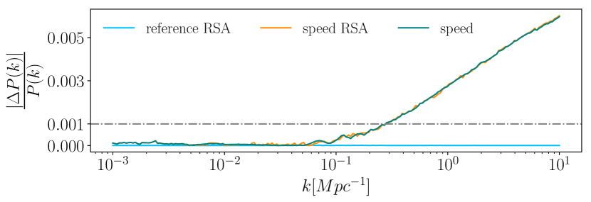
(a) Relative difference between PyCosmo reference and speed settings with (orange) and without (green) RSA.

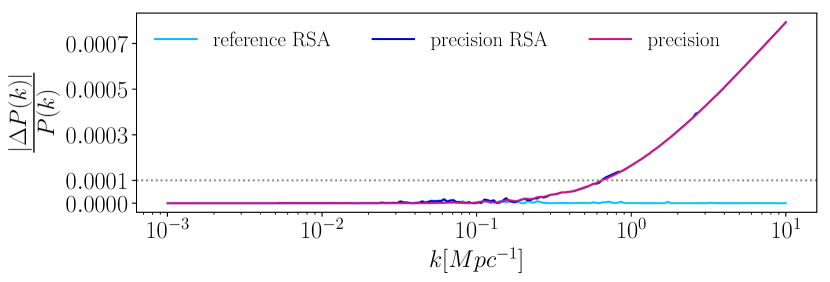
(b) Relative difference between PyCosmo reference and precision settings with (blue) and without (purple) RSA.

Figure 5: Relative difference between the $\Lambda$CDM matter power spectrum computed with l_max = 200 and atol = rtol = $10^{-6}$ (reference) and the same power spectrum computed with PyCosmo speed (top panel) and precision (bottom panel) settings with and without RSA. We also display in both panels in light blue the relative difference between the reference matter power spectrum with and without RSA. The grey horizontal lines correspond to a $10^{-3}$ (dash-dotted) and $10^{-4}$ (dotted) precision level.

Reducing the l_max parameter to 50 (precision settings) increases the discrepancy with the reference power spectrum to $\sim$0.08% for the full system, regardless of whether the RSA is turned on or not. For the speed settings, the discrepancy is $\sim$0.6% both when using or not using the RSA. The computation time is again reduced by roughly 80% when using RSA compared to solving the full equation system with the same l_max, meaning that the approximation is essential to reduce the computational time of the perturbations for mid to high $k$ values without sacrificing the accuracy. The unphysical reflection of power caused by the hierarchy truncation dominates on small scales, making the inaccuracy introduced by the approximation completely negligible.

6 Agreement and performance comparison with CLASS

In this section, we present benchmarks of the PyCosmo Boltzmann solver for all the models described in the previous sections, both in terms of relative difference to CLASS and in terms of computing times. The cosmological parameters that are modified in each model are specified in the $\Lambda$CDM, $w$CDM and degenerate $\Sigma m_{\nu}$ = 60 meV parameter settings in the previous sections, while the fixed parameters are reported in D. In order to perform a comparison purely on the Boltzmann solver, we read in the CLASS recombination files for each model and set the same initial conditions. All the computations are carried out on a single core on a full node of the ETH Zurich Euler cluster, by disabling parallel execution in CLASS and not enabling parallel computation for the PyCosmo power spectrum. We run on a full node on the cluster, instead of on a laptop, in order to only run the Boltzmann solver and not get impacted by other processes being executed by the operating system. In the case of PyCosmo, we only report the time necessary for the power spectrum computation, which does not include the compilation time for the first time the C/C++ code is generated for each model. Most models also require a second compilation (recompilation) that applies permutations to the existing equations in order to enable the use of specialized solvers instead of the standard solver as explained in Section 2.1. The runtime we report is the best time obtained in three executions.

We begin by comparing the runtime between the computation of the matter power spectrum in PyCosmo, with and without turning on the RSA, and CLASS, both for the speed and precision settings (defined in Section 2.3). In Table 2, we display the time necessary to compute the power spectrum with PyCosmo and CLASS for a 100 log-spaced $k$ values between $k_{min}$ and $k_{max}$. We fix $k_{min}$ = $10^{-4}\ \mathrm{Mpc^{-1}}$, and set $k_{max}$ first to $1\ \mathrm{Mpc^{-1}}$ and then to $10\ \mathrm{Mpc^{-1}}$, where the effects of the Radiation Streaming Approximation are most evident.

Model	$k_{max}$	Speed settings, time [s]			Precision settings, time [s]
		PyCosmo	PyCosmo RSA	CLASS	PyCosmo	PyCosmo RSA	CLASS
$\Lambda$CDM	1 $\mathrm{Mpc^{-1}}$	1.26	0.23	0.42	3.80	1.05	2.02
$\Lambda$CDM	10 $\mathrm{Mpc^{-1}}$	8.80	0.44	0.80	20.5	2.20	5.28
$w$CDM	1 $\mathrm{Mpc^{-1}}$	1.32	0.65	1.29	3.84	1.55	2.86
$w$CDM	10 $\mathrm{Mpc^{-1}}$	9.08	0.82	4.91	20.93	2.72	10.18
degenerate $M_{\nu}$	1 $\mathrm{Mpc^{-1}}$	54.54	29.04	10.19	237.26	154.93	105.87
degenerate $M_{\nu}$	10 $\mathrm{Mpc^{-1}}$	357.24	98.52	13.78	1337.32	471.22	417.95

Table 2: Best execution time from three executions on a full Euler VI node.

We observe that, while PyCosmo achieves a slower runtime than CLASS before introducing the RSA, the RSA reverts the situation for all the models, except for massive neutrinos. This happens despite the presence of further approximations in the CLASS implementation. Previous versions of PyCosmo achieved a comparable execution time with CLASS without physical approximations [Refregier et al., 2018]. This was due to the reduction of the dynamic range of the time step based on a consistency relation of the Einstein equations. The adaptive control of the time step was highly optimized for $\Lambda$CDM and proved difficult to extend to more general models. The new approach has also the advantage of reducing the number of permutations necessary to create the optimized code.

In the case of massive neutrinos, the size of the system determines a considerable decline in the performance of both codes. PyCosmo is significantly slower than CLASS when using the speed settings, mainly due to the presence of the fluid approximation for non cold dark matter in CLASS. For the $precision$ settings, the time needed for the computation is comparable for CLASS and PyCosmo. The ODE system used by CLASS is larger in this case, since the tol_ncdm parameters are set to $10^{-10}$ in pk_ref.pre, and the three neutrinos are treated independently despite having the same mass. We do not decrease mnu_relerr, equivalent to tol_ncdm, in PyCosmo since we do not deem it necessary to achieve the desired precision. The error caused by sampling less $q$ values is always subdominant compared to the hierarchy truncation, due to the small contribution of massive neutrinos to the overall matter density.

We compare the numerical results of PyCosmo and CLASS in Table 3. We report the maximum relative difference between the matter power spectra in PyCosmo and CLASS in five $k$ ranges for the different models and precision settings. The RSA is not relevant here because it leads to a $10^{-5}$ relative difference, when compared to the full computation with the same l_max, as shown for $\Lambda$CDM in the previous section.

Model	precision	$k$ range [$\mathrm{Mpc^{-1}}$]
		$10^{-4}-10^{-3}$	$10^{-3}-10^{-2}$	$10^{-2}-10^{-1}$	$10^{-1}-1$	$1-10$
$\Lambda$CDM	speed	$0.0006$	$0.0007$	$0.0007$	$0.0031$	$0.0077$
	precision	$0.0001$	$0.0003$	$0.0005$	$0.0003$	$0.0008$
$w$CDM	speed	$0.0006$	$0.0007$	$0.0008$	$0.0031$	$0.0078$
	precision	$0.0002$	$0.0003$	$0.0005$	$0.0003$	$0.0008$
degenerate $M_{\nu}$	speed	$0.0004$	$0.0010$	$0.0010$	$0.0046$	$0.0146$
	precision	$0.0001$	$0.0003$	$0.0005$	$0.0002$	$0.0001$

Table 3: Maximum relative differences in $k$ ranges between PyCosmo and CLASS for given models and precision settings.

We start by noting that the size of the relative differences is comparable in all models when using the same $k$ ranges, with the exception of the model with massive neutrinos for $k>0.1\ \mathrm{Mpc^{-1}}$. We also see that the difference in precision between speed and precision settings is dominant on scales $k>0.1\ \mathrm{Mpc^{-1}}$, where the truncation effects have the largest impact. The precision settings lead to a relative difference to CLASS that is better than $0.1\%$ on all scales $k<10\ \mathrm{Mpc^{-1}}$, while the speed settings lead to a relative difference of order $0.5-1\%$ beyond $k=0.1\ \mathrm{Mpc^{-1}}$. This is acceptable, especially since cl_permille.pre comes with no guarantees for scales $k>1\ h\mathrm{Mpc^{-1}}$.

7 Conclusion

In this paper, we demonstrated how the PyCosmo Boltzmann solver can be easily modified to include extensions of the $\Lambda$CDM cosmological model and approximation schemes, by taking advantage of the SymPy symbolic implementation of equations. The symbolic expressions are translated into optimized C/C++ code by the sympy2c package presented in Schmitt et al. [2022]. In this way, PyCosmo combines the speed of C/C++ with the user-friendliness of symbolic Python.

We first presented two cosmological model extensions: dark energy with a constant equation of state, which is a minimal modification of $\Lambda$CDM, and massive neutrinos, which enlarge considerably the ODE system and comprise numerical integrations, constituting a more complex extension. The inclusion of these models makes PyCosmo more widely applicable for constraining cosmology. We also implemented an approximation scheme, the radiation streaming approximation. In order to trigger the approximation, sympy2c includes a functionality to switch between two different ODE systems when a condition is verified. The radiation streaming approximation makes the solution of the ODE system considerably faster, up to an 80% speed-up, since it suppresses oscillations of the radiation fields for large $k$ values. The errors introduced by the approximation are largely sub-dominant compared to the artificial power reflection induced by the hierarchy truncation. For convenience, we presented a conversion table between common conventions for cosmological perturbations (A) and a clarification of the computation of the total matter power spectrum with $A_{s}$ normalization (E).

We compared the numerical results obtained by computing the total matter power spectrum with CLASS and found an agreement better than 0.1% with high precision settings. With more relaxed precision settings, we found an agreement of 0.5% for scales $k<1\mathrm{Mpc^{-1}}$ for all models. The PyCosmo Boltzmann solver achieves precision and speed that is comparable to CLASS, while not relying on physical approximations (such as tight coupling and ultra relativistic fluid approximation) other than the radiation streaming approximation introduced in this work. In the future, we plan to include more beyond $\Lambda$CDM models in PyCosmo. Possible extensions include time-varying dark energy, early dark energy [Poulin et al., 2019, Hill et al., 2020], curvature [Pitrou et al., 2020], dark matter models [Hui, 2021], such as axions and fuzzy dark matter, and extensions of the neutrino sector. We believe that our symbolic implementation will be applicable for most model extensions, with some refactoring needed when a model introduces an ODE system already at background level (for example in the case of scalar field models).

8 Acknowledgements

This work was supported in part by grant 200021_192243 from the Swiss National Science Foundation. The authors thank Thomas Tram for answering questions about the CLASS implementation. We thank Joel Mayor for his comments that led to some corrections and clean up of the code, and Silvan Fischbacher for helpful discussions. The authors also thank Joel Akeret, Adam Amara, Lukas Gamper, Jörg Herbel, Tomasz Kacprzak and Andrina Nicola for discussions and contributions to earlier versions of PyCosmo. In this work, we rely on the Python packages numpy [van der Walt et al., 2011], scipy [Virtanen et al., 2020], matplotlib [Hunter, 2007] and SymPy [Meurer et al., 2017].

Appendix A Notation table

Ma-Bertschinger	PyCosmo	Meaning
$a$	$a$	scale factor
$k$	$k$	wavenumber of Fourier mode
$P_{i}$	$P_{i}$	conjugate momentum to $x_{i}$
$p_{i}$	$p_{i}$	proper momentum
$q_{i}$	$q_{i}$	$ap_{i}$
$\epsilon_{i}$	$\epsilon_{i}$	$(q_{i}^{2}+am^{2})^{1/2}$
$\delta_{\gamma}$	$4\Theta_{0}$	photons overdensity
$\theta_{\gamma}$	$3k\Theta_{1}$	photons velocity divergence
$\sigma_{\gamma}$	$2\Theta_{2}$	photons shear stress
$F_{\gamma l}$	$4\Theta_{l}$	$l$th Legendre component of photons perturbations
$\delta_{ur}$	$4\mathcal{N}_{0}$	massless neutrinos overdensity
$\theta_{ur}$	$3k\mathcal{N}_{1}$	divergence of massless neutrinos velocity
$\sigma_{ur}$	$2\mathcal{N}_{2}$	shear stress of massless neutrino fluid
$\psi,\phi$	$\Psi,-\Phi$	Newtonian gravitational potentials
$\tau$	$\eta$	conformal time
$\tau_{c}$=1/$\kappa^{\prime}$	$-\dot{\tau}$	Thomson scattering rate
$\theta_{c}$	$ku=ikv$	velocity divergence of dark matter
$\theta_{b}$	$ku_{b}=ikv_{b}$	velocity divergence of baryons
$\Psi_{1},\Psi_{2},\Psi_{l}$	$\mathcal{M}_{1},\mathcal{M}_{2},\mathcal{M}_{l}$	Legendre components of massive neutrinos perturbations
$\delta_{h}$	$\delta_{\nu,m}$	massive neutrinos overdensity
$\theta_{h}$	$ku_{\nu,m}$	massive neutrinos velocity divergence
$\sigma_{h}$	$\sigma_{\nu,m}$	massive neutrinos shear stress

Table 4: Relations between the notation in Ma-Bertschinger and PyCosmo. Ma-Bertschinger notation is used in both the Boltzmann solvers COSMICS and CLASS. Some exceptions include $\theta_{ur}$ that is denoted $\theta_{r}$ in COSMICS and all the massive neutrino quantities that are denoted $\delta_{ncdm},\ \theta_{ncdm}$ and $\sigma_{ncdm}$ in CLASS (ncdm = non cold dark matter) and $\delta_{n},\ \theta_{n}$ and $\sigma_{n}$ in COSMICS.

Appendix B Linear perturbations in $\ln(a)$

In PyCosmo we use $\ln(a)$ (from here on simply $lna$) as the independent variable of the Einstein-Boltzmann ODE system. The relation between $\ln(a)$ and $\eta$ is simply: $\frac{d\ln(a)}{d\eta}=aH$. We report the Einstein-Boltzmann equations in $\Lambda$CDM, as used in the code, in the following:

• Einstein equations:

  $$\Psi =-\Phi-12\left(\frac{H_{0}}{ka}\right)^{2}\left(\Omega_{\gamma}\Theta_{2}+\Omega_{\nu}\mathcal{N}_{2}\right)$$

  $$\Pi =\Theta_{2}+\Theta_{P,0}+\Theta_{P,2}$$

  $$\frac{d\Phi}{dlna} =\Psi-\left(\frac{k}{aH}\right)^{2}\frac{\Phi}{3}+\frac{1}{2}\left(\frac{H_{0}}{H}\right)^{2}\left(\left(\Omega_{dm}\delta+\Omega_{b}\delta_{b}\right)a^{-3}+4a^{-4}\left(\Omega_{\gamma}\Theta_{0}+\Omega_{\nu}\mathcal{N}_{0}\right)\right)$$

• Dark matter:

  $$\frac{d\delta}{dlna} =-\frac{k}{aH}u-3\frac{d\Phi}{dlna}$$

  $$\frac{du}{dlna} =-u+\frac{k}{aH}\Psi$$

• Baryonic matter:

  $$\frac{d\delta_{b}}{dlna} =-\frac{k}{aH}u_{b}-3\frac{d\Phi}{dlna}$$

  $$\frac{du_{b}}{dlna} =-u_{b}+\frac{k}{aH}\Psi+\frac{\dot{\tau}}{RaH}\left(u_{b}-3\Theta_{1}\right)+\frac{k}{aH}{c_{s}}^{2}\delta_{b}$$

• Photons temperature:

  $$\frac{d\Theta_{0}}{dlna} =-\frac{k}{aH}\Theta_{1}-\frac{d\Phi}{dlna}$$

  $$\frac{d\Theta_{1}}{dlna} =\frac{k}{3aH}\left(\Theta_{0}-2\Theta_{2}+\Psi\right)+\frac{\dot{\tau}}{aH}\left(\Theta_{1}-\frac{u_{b}}{3}\right)$$

  $$\frac{d\Theta_{2}}{dlna} =\frac{k}{5aH}\left(2\Theta_{1}-3\Theta_{3}\right)+\frac{\dot{\tau}}{aH}\left(\Theta_{P,0}-\frac{\Pi}{2}\right)$$

  For $l>2$

  $$\frac{d\Theta_{l}}{dlna}=\frac{k}{aH(2l+1)}\left(l\Theta_{l-1}-(l+1)\Theta_{l+1}\right)+\frac{\dot{\tau}}{aH}\Theta_{l}$$

• Photons polarization:

  $$\frac{d\Theta_{P,0}}{dlna} =-\frac{k}{aH}\Theta_{P,1}+\frac{\dot{\tau}}{aH}\left(\Theta_{P,0}-\frac{\Pi}{2}\right)$$

  $$\frac{d\Theta_{P,1}}{dlna} =\frac{k}{3aH}\left(\Theta_{P,0}-2\Theta_{P,2}\right)+\frac{\dot{\tau}}{aH}\Theta_{P,1}$$

  $$\frac{d\Theta_{P,2}}{dlna} =\frac{k}{5aH}\left(2\Theta_{P,1}-3\Theta_{P,3}\right)+\frac{\dot{\tau}}{aH}\left(\Theta_{P,2}-\frac{\Pi}{10}\right)$$

  For $l>2$

  $$\frac{d\Theta_{P,l}}{dlna}=\frac{k}{aH(2l+1)}\left(l\Theta_{P,l-1}-(l+1)\Theta_{P,l+1}\right)+\frac{\dot{\tau}}{aH}\Theta_{P,l}$$

• Massless neutrinos:

  $$\frac{d\mathcal{N}_{0}}{dlna} =-\frac{k}{aH}\mathcal{N}_{1}-\frac{d\Phi}{dlna}$$

  $$\frac{d\mathcal{N}_{1}}{dlna} =\frac{k}{3aH}\left(\mathcal{N}_{0}-2\mathcal{N}_{2}+\Psi\right)$$

  For $l\geq 2$

  $$\frac{d\mathcal{N}_{l}}{dlna}=\frac{k}{(2l+1)aH}\left(l\mathcal{N}_{l-1}-(l+1)\mathcal{N}_{l+1}\right)$$

  The hierarchy truncations for relativistic species read:

  $$\frac{d\Theta_{l_{max}}}{dlna} =\frac{1}{aH}\left(k\Theta_{l_{max}-1}-\left(\frac{(l_{max}+1)}{\eta}-\dot{\tau}\right)\Theta_{l_{max}}\right)$$

  $$\frac{d\Theta_{P,l_{max}}}{dlna} =\frac{1}{aH}\left(k\Theta_{P,l_{max}}-\left(\frac{(l_{max}+1)}{\eta}-\dot{\tau}\right)\Theta_{P,l_{max}}\right)$$

  $$\frac{d\mathcal{N}_{l_{max}}}{dlna} =\frac{1}{aH}\left(k\mathcal{N}_{l_{max}-1}-\frac{l_{max}+1}{\eta}\mathcal{N}_{l_{max}}\right)$$

The equations for the extended models are easily obtained with the same change of variables from the equations in $\eta$, reported in the corresponding sections of the paper.

Appendix C Adiabatic initial conditions

The default setting of PyCosmo is to use the adiabatic initial conditions from CLASS [Blas et al., 2011, Cyr-Racine & Sigurdson, 2011, Bucher et al., 2000]. We present the initial conditions for $\Lambda$CDM, wCDM and massive neutrinos in the following. We start by introducing auxiliary notation which is useful to define the initial conditions:

$$\eta_{0} =\eta(a_{0})\hskip 93.89418pt\frac{\dot{a}}{a} =aH(a_{0})\hskip 56.9055pt\omega =\frac{\Omega_{m}H_{0}}{\sqrt{\Omega_{r,tot}}}\hskip 56.9055pt\frac{\rho_{m}}{\rho_{r}} =\frac{\Omega_{m}a_{0}}{\Omega_{r}}$$

$$F_{\nu} =\frac{\Omega_{\nu,tot}}{\Omega_{r,tot}}\hskip 79.6678ptF_{cdm} =\frac{\Omega_{cdm}}{\Omega_{m}}\hskip 56.9055ptF_{b} =1-F_{cdm}\hskip 56.9055ptF_{g} =1-F_{\nu}$$

where $\Omega_{\nu,tot}=\frac{7}{8}N_{\mathrm{eff}}\left(\frac{4}{11}\right)^{\frac{4}{3}}\Omega_{\gamma}$ which includes massless and massive neutrinos (assumed to be relativistic at early times), $\Omega_{r,tot}=\Omega_{\gamma}+\Omega_{\nu,tot}$ and $\eta_{0}$ is defined as the minimum between $0.001/k$ and $0.1h$ with $k$ expressed in $h$Mpc^-1. $a_{0}$ is computed from $\eta_{0}$ assuming radiation domination as $a_{0}=\eta_{0}\sqrt{\Omega_{r,tot}}/H_{0}$. We use these conservative definitions of initial times to avoid using an iterative shooting algorithm. The initial perturbations are computed in synchronous gauge as

$$\delta_{g} =-\frac{(k\eta_{0})^{2}(1-\frac{\omega\eta_{0}}{5})}{3}$$

$$\theta_{g} =-\frac{k(k\eta_{0})^{3}}{36}\left(1-\frac{3(1+5F_{b}-F_{\nu})}{20(1-F_{\nu})}\omega\eta_{0}\right)$$

$$\delta_{b} =\frac{3\delta_{g}}{4}=\delta_{c}$$

$$\theta_{b} =\theta_{g}$$

$$\delta_{ur} =\delta_{g}$$

$$\theta_{ur} =-\frac{k(k\eta_{0})^{3}}{36(4F_{\nu}+15)}\left(4F_{\nu}+23-\frac{3(8F_{\nu}^{2}+50F_{\nu}+275)}{20(2F_{\nu}+15)}\eta_{0}\omega\right)$$

$$\sigma_{ur} =\frac{2(k\eta_{0})^{2}}{45+12F_{\nu}}\left(1+\frac{(4F_{\nu}-5)}{4(2F_{\nu}+15)}\eta_{0}\omega\right)$$

$$l3_{ur} =\frac{2(k\eta_{0})^{3}}{7(12F_{\nu}+45)}$$

$$\eta_{sync} =1-\frac{(k\eta_{0})^{2}}{12(15+4F_{\nu})}(5+4F_{\nu}-\frac{(16F_{\nu}^{2}+280F_{\nu}+325)}{10(2F_{\nu}+15)}\eta_{0}\omega).$$

In the wCDM case we add the generalized initial adiabatic conditions from Ballesteros & Lesgourgues [2010] for the dark energy fields:

$$\delta_{\mathrm{de}} =-\frac{1}{4}(1+w_{\mathrm{de}})\frac{4-3c_{\mathrm{s,de}}^{2}}{4-6w_{\mathrm{de}}+3c_{\mathrm{s,de}}^{2}}(k\eta_{0})^{2}$$

$$\theta_{\mathrm{de}} =-\frac{kc_{\mathrm{s,de}}^{2}}{4(4-6w_{\mathrm{de}}+3c_{\mathrm{s,de}}^{2})}(k\eta_{0})^{3}.$$

We then need to introduce the transformation from synchronous to conformal Newtonian gauge that uses the following quantities

$$\delta_{tot} =\frac{F_{g}\delta_{g}+F_{\nu}\delta_{ur}+\frac{\rho_{m}}{\rho_{r}}(F_{b}\delta_{b}+F_{cdm}\delta_{c})}{1+\frac{\rho_{m}}{\rho_{r}}}$$

$$v_{tot} =\frac{\frac{4}{3}(F_{g}\theta_{g}+F_{\nu}\theta_{ur})+\frac{\rho_{m}}{\rho_{r}}F_{b}\theta_{b}}{(1+\frac{\rho_{m}}{\rho_{r}})}$$

$$\alpha =\frac{\eta_{sync}+\frac{3}{2}\left(\frac{\dot{a}}{a}\right)^{2}\frac{1}{k^{2}}(\delta_{tot}+3\frac{\dot{a}}{a}\frac{v_{tot}}{k^{2}})}{\frac{\dot{a}}{a}}$$

and reads

$$-\Phi =\eta_{sync}-\frac{\dot{a}}{a}\alpha$$

$$\delta_{c} =\delta_{c}(sync)-3\frac{\dot{a}}{a}\alpha \theta_{c} =k^{2}\alpha$$

$$\delta_{b} =\delta_{b}(sync)-3\frac{\dot{a}}{a}\alpha \theta_{b} =\theta_{b}(sync)+k^{2}\alpha$$

$$\delta_{g} =\delta_{g}(sync)-4\frac{\dot{a}}{a}\alpha \theta_{g} =\theta_{g}(sync)+k^{2}\alpha$$

$$\delta_{ur} =\delta_{ur}(sync)-4\frac{\dot{a}}{a} \theta_{ur} =\theta_{ur}(sync)+k^{2}\alpha$$

$$\delta_{\mathrm{de}} =\delta_{\mathrm{de}}(sync)-3(1+w_{\mathrm{de}})\frac{\dot{a}}{a}\alpha \theta_{\mathrm{de}} =\theta_{\mathrm{de}}(sync)+k^{2}\alpha.$$

The fields where we did not specify a conversion are gauge invariant, including the massive neutrinos’ perturbations of the distribution function. The initial conditions imposed to the multipoles of $\mathcal{M}(\mu)$ are

$$\mathcal{M}_{0} =-\frac{1}{4}\delta_{\nu}\frac{dlnf_{0}}{d\ln{q}}=\frac{q}{k_{b}T_{0}}\frac{\mathcal{N}_{0}}{e^{-q/k_{b}T_{0}}+1}$$

$$\mathcal{M}_{1} =-\frac{\epsilon}{3qk}\theta_{\nu}\frac{dlnf_{0}}{d\ln{q}}=\frac{\epsilon}{k_{b}T_{0}}\frac{\mathcal{N}_{1}}{e^{-q/k_{b}T_{0}}+1}$$

$$\mathcal{M}_{2} =-\frac{1}{2}\sigma_{\nu}\frac{dlnf_{0}}{d\ln{q}}=\frac{q}{k_{b}T_{0}}\frac{\mathcal{N}_{2}}{e^{-q/k_{b}T_{0}}+1}$$

$$\mathcal{M}_{3} =-\frac{1}{4}l3_{ur}\frac{dlnf_{0}}{d\ln{q}}=\frac{q}{k_{b}T_{0}}\frac{\mathcal{N}_{3}}{e^{-q/k_{b}T_{0}}+1}$$

and are set after transforming the other fields to the conformal Newtonian gauge. We can then relate the fields from CLASS to those of PyCosmo with the following conversions (already introduced in Appendix A):

$$u =\theta_{c}/k u_{b} =\theta_{b}/k u_{\mathrm{de}} =\theta_{\mathrm{de}}/k \Theta_{0} =\delta_{g}/4 \mathcal{N}_{0} =\delta_{ur}/4$$

$$\Theta_{1} =\theta_{g}/3k \mathcal{N}_{1} =\theta_{ur}/3k \mathcal{N}_{2} =\sigma_{ur}/2 \mathcal{N}_{3} =l3_{ur}/4.$$

Appendix D Fixed cosmological parameters

We report all the parameters of the configuration file of PyCosmo that are kept fixed throughout the paper:

[cosmology]
h = 0.7
omega_b = 0.06
flat_universe = True
Tcmb = 2.725
Yp = 0.24
wa = 0.0
cs_de2 = 1.0
T_mnu = 0.71611

[recombination]
recomb = ‘class’

[linear_perturbations]
pk_type = ‘boltz’
pk_norm_type = ‘A_s’
pk_norm = 2.1e-9
k_pivot = 0.05

[internal:boltzmann_solver]
initial_conditions = ‘class’
dt_0 = 1.5e-2
sec_factor = 10.0
boltzmann_max_bdf_order = 5
boltzmann_max_iter = 10000000
fast_solver = True

[internal:physical_constants]
kb = 8.617342790900664e-05
evc2 = 1.7826617580683397e-36
G = 6.67428e-11
hbar = 6.582118991312934e-16
mpc = 3.085677581282e22
mp = 938.272013425824
msun = 1.98855e30
sigmat = 6.6524616e-29

Note that the physical constants are not set to the default values in PyCosmo, but to default values from CLASS (found in the header files thermodynamics.h and background.h).

The same parameters are passed to CLASS and are also fixed throughout this work:

output = ‘mPk’
T_cmb = 2.725
Omega_b = 0.06
h = 0.7
T_ncdm =  0.71611, 0.71611, 0.71611
ksi_ncdm = 0, 0, 0
Omega_fld = 0
wa_fld = 0
cs2_fld = 1
reio_parametrization = ‘reio_none’
YHe = 0.24
gauge = ‘newtonian’
A_s = 2.1e-09
n_s = 1
alpha_s = 0
k_pivot = 0.05

Note that some parameters (for instance $T_{\nu,m}$ or $c^{2}_{s,de}$) are specified only when necessary.

Appendix E Power spectrum computation

We compute the gauge invariant real space matter power spectrum, using a fully general relativistic treatment [Yoo et al., 2009, Yoo, 2010, Bonvin & Durrer, 2011, Challinor & Lewis, 2011], accounting for real space matter fluctuations and volume distortions, similarly to CLASS [Dio et al., 2013]. Note that general relativistic corrections are not included in other observables in PyCosmo, but are left as future development. Prior versions of PyCosmo separated transfer function and growth factor and used the Poisson equation to relate the Newtonian gauge matter density perturbation to the Newtonian gravitational potential. This is still the case when setting pk_norm_type to deltah and using the power spectrum fitting functions.

We define $\Omega_{m,tot}=\Omega_{dm}+\Omega_{b}+\Omega_{\nu,m}$ as the total matter energy density, including massive neutrinos and $P_{m,tot}=P_{\nu,m}$, since the massive neutrino component is the only matter ingredient that has a non-zero pressure term. Then the gauge invariant matter density reads

$$\begin{split}\delta_{m,tot}=\frac{\delta\rho_{m,tot}}{\bar{\rho}_{m,tot}}+3\frac{aH}{k^{2}}\theta_{m,tot}=\ &\frac{\Omega_{dm}\delta+\Omega_{b}\delta_{b}+\Omega_{\nu,m}\delta_{\nu,m}}{\Omega_{m,tot}}\\ &+3\frac{aH}{k}\frac{\Omega_{dm}u+\Omega_{b}u_{b}+(\Omega_{\nu,m}+P_{\nu,m})u_{\nu,m}}{\Omega_{m,tot}+P_{m,tot}},\end{split}$$ (22)

where we omitted the $a$ dependencies for brevity.

The power spectrum is defined in terms of the primordial power spectrum of gauge invariant curvature perturbations, $P_{\mathcal{R}}(k)=\mathcal{A}_{s}\left(\frac{k}{k_{p}}\right)^{n_{s}-1}$ with $n_{s}$ the tilt of the primordial power spectrum and $k_{p}$ the pivot scale with corresponding $\mathcal{A}_{s}$ amplitude , as

$$P(k,a)=2\pi^{2}\mathcal{A}_{s}\frac{k^{n_{s}-4}}{k_{p}^{n_{s}-1}}\delta_{m,tot}(k,a)^{2},$$ (23)

valid in the case of adiabatic initial conditions for which the initial curvature $\mathcal{R}$ is normalized to 1. These are the only initial conditions currently implemented in PyCosmo. PyCosmo also allows to output $P_{cb}(k,a)$, the power spectrum of dark and baryonic matter, where massive neutrinos are excluded.

References

- Abbott et al. [2021] Abbott, T. M. C. et al. (DES) (2021). Dark Energy Survey Year 3 Results: Cosmological Constraints from Galaxy Clustering and Weak Lensing, . arXiv:2105.13549.
- Aghanim et al. [2020] Aghanim, N. et al. (Planck) (2020). Planck 2018 results. VI. Cosmological parameters. Astron. Astrophys., 641, A6. doi:10.1051/0004-6361/201833910. arXiv:1807.06209.
- Ahmad et al. [2002] Ahmad, Q. R. et al. (SNO Collaboration) (2002). Direct evidence for neutrino flavor transformation from neutral-current interactions in the sudbury neutrino observatory. Phys. Rev. Lett., 89, 011301. URL: https://link.aps.org/doi/10.1103/PhysRevLett.89.011301. doi:10.1103/PhysRevLett.89.011301.
- Ballesteros & Lesgourgues [2010] Ballesteros, G., & Lesgourgues, J. (2010). Dark energy with non-adiabatic sound speed: initial conditions and detectability. JCAP, 10, 014. doi:10.1088/1475-7516/2010/10/014. arXiv:1004.5509.
- Bertschinger [1995] Bertschinger, E. (1995). COSMICS: Cosmological Initial Conditions and Microwave Anisotropy Codes. arXiv e-prints, (pp. astro--ph/9506070). arXiv:astro-ph/9506070.
- Blas et al. [2011] Blas, D., Lesgourgues, J., & Tram, T. (2011). The cosmic linear anisotropy solving system (class). part ii: Approximation schemes. Journal of Cosmology and Astroparticle Physics, 2011, 034–034. URL: http://dx.doi.org/10.1088/1475-7516/2011/07/034. doi:10.1088/1475-7516/2011/07/034.
- Bonvin & Durrer [2011] Bonvin, C., & Durrer, R. (2011). What galaxy surveys really measure. Physical Review D, 84. URL: http://dx.doi.org/10.1103/PhysRevD.84.063505. doi:10.1103/physrevd.84.063505.
- Bucher et al. [2000] Bucher, M., Moodley, K., & Turok, N. (2000). General primordial cosmic perturbation. Physical Review D, 62. URL: https://doi.org/10.1103%2Fphysrevd.62.083508. doi:10.1103/physrevd.62.083508.
- Challinor & Lewis [2011] Challinor, A., & Lewis, A. (2011). Linear power spectrum of observed source number counts. Physical Review D, 84. URL: http://dx.doi.org/10.1103/PhysRevD.84.043516. doi:10.1103/physrevd.84.043516.
- Chisari et al. [2019] Chisari, N. E. et al. (LSST Dark Energy Science) (2019). Core Cosmology Library: Precision Cosmological Predictions for LSST. Astrophys. J. Suppl., 242, 2. doi:10.3847/1538-4365/ab1658. arXiv:1812.05995.
- Cyr-Racine & Sigurdson [2011] Cyr-Racine, F.-Y., & Sigurdson, K. (2011). Photons and baryons before atoms: Improving the tight-coupling approximation. Physical Review D, 83. URL: https://doi.org/10.1103%2Fphysrevd.83.103521. doi:10.1103/physrevd.83.103521.
- Dio et al. [2013] Dio, E. D., Montanari, F., Lesgourgues, J., & Durrer, R. (2013). The classgal code for relativistic cosmological large scale structure. Journal of Cosmology and Astroparticle Physics, 2013, 044–044. URL: http://dx.doi.org/10.1088/1475-7516/2013/11/044. doi:10.1088/1475-7516/2013/11/044.
- Dodelson [2003] Dodelson, S. (2003). Modern Cosmology. Academic Press, Elsevier Science.
- Doran [2005a] Doran, M. (2005a). Cmbeasy: an object oriented code for the cosmic microwave background. Journal of Cosmology and Astroparticle Physics, 2005, 011–011. URL: http://dx.doi.org/10.1088/1475-7516/2005/10/011. doi:10.1088/1475-7516/2005/10/011.
- Doran [2005b] Doran, M. (2005b). Speeding up cosmological Boltzmann codes. JCAP, 06, 011. doi:10.1088/1475-7516/2005/06/011. arXiv:astro-ph/0503277.
- Eguchi et al. [2003] Eguchi, K. et al. (KamLAND Collaboration) (2003). First results from kamland: Evidence for reactor antineutrino disappearance. Phys. Rev. Lett., 90, 021802. URL: https://link.aps.org/doi/10.1103/PhysRevLett.90.021802. doi:10.1103/PhysRevLett.90.021802.
- Eisenstein & Hu [1998] Eisenstein, D. J., & Hu, W. (1998). Baryonic features in the matter transfer function. The Astrophysical Journal, 496, 605–614. URL: http://dx.doi.org/10.1086/305424. doi:10.1086/305424.
- Fukuda et al. [1998] Fukuda, Y. et al. (Super-Kamiokande Collaboration) (1998). Evidence for oscillation of atmospheric neutrinos. Phys. Rev. Lett., 81, 1562--1567. URL: https://link.aps.org/doi/10.1103/PhysRevLett.81.1562. doi:10.1103/PhysRevLett.81.1562.
- Hill et al. [2020] Hill, J. C., McDonough, E., Toomey, M. W., & Alexander, S. (2020). Early dark energy does not restore cosmological concordance. Phys. Rev. D, 102, 043507. doi:10.1103/PhysRevD.102.043507. arXiv:2003.07355.
- Hu et al. [2014] Hu, B., Raveri, M., Frusciante, N., & Silvestri, A. (2014). Effective Field Theory of Cosmic Acceleration: an implementation in CAMB. Phys. Rev. D, 89, 103530. doi:10.1103/PhysRevD.89.103530. arXiv:1312.5742.
- Hui [2021] Hui, L. (2021). Wave Dark Matter, . arXiv:2101.11735.
- Hunter [2007] Hunter, J. D. (2007). Matplotlib: A 2d graphics environment. Computing in Science & Engineering, 9, 90--95. doi:10.1109/MCSE.2007.55.
- Ichikawa et al. [2005] Ichikawa, K., Fukugita, M., & Kawasaki, M. (2005). Constraining neutrino masses by CMB experiments alone. Phys. Rev. D, 71, 043001. doi:10.1103/PhysRevD.71.043001. arXiv:astro-ph/0409768.
- Lattanzi & Gerbino [2018] Lattanzi, M., & Gerbino, M. (2018). Status of neutrino properties and future prospects - Cosmological and astrophysical constraints. Front. in Phys., 5, 70. doi:10.3389/fphy.2017.00070. arXiv:1712.07109.
- Lesgourgues [2011a] Lesgourgues, J. (2011a). The Cosmic Linear Anisotropy Solving System (CLASS) I: Overview. Technical Report CERN. URL: [arXiv:1104.2932].
- Lesgourgues [2011b] Lesgourgues, J. (2011b). The cosmic linear anisotropy solving system (class) iii: Comparision with camb for lambdacdm. arXiv:1104.2934.
- Lesgourgues et al. [2013] Lesgourgues, J., Mangano, G., Miele, G., & Pastor, S. (2013). Neutrino Cosmology. Cambridge University Press. doi:10.1017/CBO9781139012874.
- Lesgourgues & Pastor [2006] Lesgourgues, J., & Pastor, S. (2006). Massive neutrinos and cosmology. Phys. Rept., 429, 307--379. doi:10.1016/j.physrep.2006.04.001. arXiv:astro-ph/0603494.
- Lesgourgues & Tram [2011] Lesgourgues, J., & Tram, T. (2011). The cosmic linear anisotropy solving system (class) iv: efficient implementation of non-cold relics. Journal of Cosmology and Astroparticle Physics, 2011, 032–032. URL: http://dx.doi.org/10.1088/1475-7516/2011/09/032. doi:10.1088/1475-7516/2011/09/032.
- Lewis et al. [2000] Lewis, A., Challinor, A., & Lasenby, A. (2000). Efficient computation of cosmic microwave background anisotropies in closed friedmann-robertson-walker models. The Astrophysical Journal, . URL: [arXiv:astro-ph/9911177].
- Ma & Bertschinger [1995] Ma, C., & Bertschinger, E. (1995). Cosmological perturbation theory in the synchronous and conformal newtonian gauges. Astrophys.J., (pp. 7--25). URL: [arXiv:astro-ph/9506072].
- Meurer et al. [2017] Meurer, A., Smith, C., Paprocki, M., Čertík, O., Kirpichev, S., Rocklin, M., Kumar, A., Ivanov, S., Moore, J., Singh, S., Rathnayake, T., Vig, S., Granger, B., Muller, R., Bonazzi, F., Gupta, H., Vats, S., Johansson, F., Pedregosa, F., & Scopatz, A. (2017). Sympy: Symbolic computing in python. PeerJ Computer Science, 3, e103. doi:10.7717/peerj-cs.103.
- Nadkarni-Ghosh & Refregier [2017] Nadkarni-Ghosh, S., & Refregier, A. (2017). The einstein–boltzmann equations revisited. Monthly Notices of the Royal Astronomical Society, 471, 2391–2430. URL: http://dx.doi.org/10.1093/mnras/stx1662. doi:10.1093/mnras/stx1662.
- Peacock [1997] Peacock, J. A. (1997). The evolution of galaxy clustering. Monthly Notices of the Royal Astronomical Society, 284, 885–898. URL: http://dx.doi.org/10.1093/mnras/284.4.885. doi:10.1093/mnras/284.4.885.
- Petzold [1983] Petzold (1983). Automatic selection of methods for solving stiff and nonstiff systems of ordinary differential equations. SIAM Journal on Scientific and Statistical Computing, 4, 136--148.
- Pitrou et al. [2020] Pitrou, C., Pereira, T. S., & Lesgourgues, J. (2020). Optimal Boltzmann hierarchies with nonvanishing spatial curvature. Phys. Rev. D, 102, 023511. doi:10.1103/PhysRevD.102.023511. arXiv:2005.12119.
- Poulin et al. [2019] Poulin, V., Smith, T. L., Karwal, T., & Kamionkowski, M. (2019). Early Dark Energy Can Resolve The Hubble Tension. Phys. Rev. Lett., 122, 221301. doi:10.1103/PhysRevLett.122.221301. arXiv:1811.04083.
- Refregier et al. [2011] Refregier, A., Amara, A., Kitching, T. D., & Rassat, A. (2011). icosmo: an interactive cosmology package. Astronomy & Astrophysics, 528, A33. URL: http://dx.doi.org/10.1051/0004-6361/200811112. doi:10.1051/0004-6361/200811112.
- Refregier et al. [2018] Refregier, A., Gamper, L., A. Amara, & Heisenberg, L. (2018). PyCosmo: An integrated cosmological boltzmann solver. Astronomy and Computing, . URL: [arXiv:1708.05177].
- de Salas et al. [2021] de Salas, P. F., Forero, D. V., Gariazzo, S., Martínez-Miravé, P., Mena, O., Ternes, C. A., Tórtola, M., & Valle, J. W. F. (2021). 2020 global reassessment of the neutrino oscillation picture. Journal of High Energy Physics, 2021. URL: http://dx.doi.org/10.1007/JHEP02(2021)071. doi:10.1007/jhep02(2021)071.
- Schmitt et al. [2022] Schmitt, U., Moser, B., Lorenz, C. S., & Refregier, A. (2022). sympy2c: from symbolic expressions to fast c/c++ functions and ode solvers in python. URL: https://arxiv.org/abs/2203.11945. doi:10.48550/ARXIV.2203.11945.
- Scolnic et al. [2018] Scolnic, D. M. et al. (2018). The Complete Light-curve Sample of Spectroscopically Confirmed SNe Ia from Pan-STARRS1 and Cosmological Constraints from the Combined Pantheon Sample. Astrophys. J., 859, 101. doi:10.3847/1538-4357/aab9bb. arXiv:1710.00845.
- Seljak & Zaldarriaga [1996] Seljak, U., & Zaldarriaga, M. (1996). A line-of-sight integration approach to cosmic microwave background anisotropies. The Astrophysical Journal, 469, 437. URL: http://dx.doi.org/10.1086/177793. doi:10.1086/177793.
- Tarsitano et al. [2021] Tarsitano, F., Schmitt, U., Refregier, A., Fluri, J., Sgier, R., Nicola, A., Herbel, J., Amara, A., Kacprzak, T., & Heisenberg, L. (2021). Predicting cosmological observables with pycosmo. Astronomy and Computing, 36, 100484. URL: https://www.sciencedirect.com/science/article/pii/S221313372100038X. doi:https://doi.org/10.1016/j.ascom.2021.100484.
- Tripathi et al. [2017] Tripathi, A., Sangwan, A., & Jassal, H. K. (2017). Dark energy equation of state parameter and its evolution at low redshift. JCAP, 06, 012. doi:10.1088/1475-7516/2017/06/012. arXiv:1611.01899.
- Virtanen et al. [2020] Virtanen, P., Gommers, R., Oliphant, T. E., Haberland, M., Reddy, T., Cournapeau, D., Burovski, E., Peterson, P., Weckesser, W., Bright, J., & et al. (2020). Scipy 1.0: fundamental algorithms for scientific computing in python. Nature Methods, 17, 261–272. URL: http://dx.doi.org/10.1038/s41592-019-0686-2. doi:10.1038/s41592-019-0686-2.
- van der Walt et al. [2011] van der Walt, S., Colbert, S. C., & Varoquaux, G. (2011). The numpy array: A structure for efficient numerical computation. Computing in Science & Engineering, 13, 22–30. URL: http://dx.doi.org/10.1109/MCSE.2011.37. doi:10.1109/mcse.2011.37.
- Yoo [2010] Yoo, J. (2010). General relativistic description of the observed galaxy power spectrum: Do we understand what we measure? Physical Review D, 82. URL: http://dx.doi.org/10.1103/PhysRevD.82.083508. doi:10.1103/physrevd.82.083508.
- Yoo et al. [2009] Yoo, J., Fitzpatrick, A. L., & Zaldarriaga, M. (2009). New perspective on galaxy clustering as a cosmological probe: General relativistic effects. Physical Review D, 80. URL: http://dx.doi.org/10.1103/PhysRevD.80.083514. doi:10.1103/physrevd.80.083514.
- Zumalacárregui et al. [2017] Zumalacárregui, M., Bellini, E., Sawicki, I., Lesgourgues, J., & Ferreira, P. G. (2017). hi_class: Horndeski in the Cosmic Linear Anisotropy Solving System. JCAP, 08, 019. doi:10.1088/1475-7516/2017/08/019. arXiv:1605.06102.