$(g-2)_{e,\,\mu}$ and strongly interacting dark matter with collider implications

Abstract

The quest for new physics beyond the Standard Model is boosted by the recently observed deviation in the anomalous magnetic moments of muon and electron from their respective theoretical prediction. In the present work, we have proposed a suitable extension of the minimal $L_{\mu}-L_{\tau}$ model to address these two experimental results as the minimal model is unable to provide any realistic solution. In our model, a new Yukawa interaction involving first generation of leptons, a singlet vector like fermion ($\chi^{\pm}$) and a scalar (either an SU(2)_L doublet $\Phi^{\prime}_{2}$ or a complex singlet $\Phi^{\prime}_{4}$) provides the additional one loop contribution to $a_{e}$ only on top of the usual contribution coming from the $L_{\mu}-L_{\tau}$ gauge boson ($Z_{\mu\tau}$) to both electron and muon. The judicious choice of $L_{\mu}-L_{\tau}$ charges to these new fields results in a strongly interacting scalar dark matter in $\mathcal{O}({\rm MeV})$ range after taking into account the bounds from relic density, unitarity and self interaction. The freeze-out dynamics of dark matter is greatly influenced by $3\rightarrow 2$ scatterings while the kinetic equilibrium with the SM bath is ensured by $2\rightarrow 2$ scatterings with neutrinos where $Z_{\mu\tau}$ plays a pivotal role. The detection of dark matter is possible directly through scatterings with nuclei mediated by the SM $Z$ bosons. Moreover, our proposed model can also be tested in the upcoming $e^{+}e^{-}$ colliders by searching opposite sign di-electron and missing energy signal i.e. $e^{+}e^{-}\rightarrow\chi^{+}\chi^{-}\rightarrow e^{+}e^{-}\cancel{E}_{T}$ at the final state.

I Introduction

The Standard Model (SM) is a very well established theory of nature and is confirmed fully with the discovery of the Higgs boson. But with time, we have understood from various astrophysical phenomena Sofue:2000jx ; Bartelmann:1999yn ; Clowe:2003tk that the matter content of the Universe is not only made up of with the elementary particles described by the SM but more than 80$\%$ matter content of the Universe is unknown to us. This mysterious part is the so called dark matter (DM), and its presence has been confirmed by many pieces of evidence from large scale to small scale observations. The most precise determination of dark matter abundance at the present epoch is $\Omega_{\rm DM}h^{2}=0.120\pm 0.001$ by the Planck satellite Planck:2018vyg . Therefore, in order to have a viable dark matter candidate(s), it is essential to extend the particle spectrum of the SM. Moreover, a long standing discrepancy exits over the last two decades between the theoretical prediction of the SM and the experimental measurement of the anomalous magnetic moment of muon Muong-2:2001kxu ; Muong-2:2006rrc ; Jegerlehner:2009ry ; Davier:2019can ; Aoyama:2020ynm . Recently, Fermilab has announced a $4.2\sigma$ discrepancy between the experimental and theoretical value Muong-2:2021ojo ,

$$\Delta a_{\mu}=a^{\rm exp}_{\mu}-a^{\rm SM}_{\mu}=\left(2.51\pm 0.59\right)\times 10^{-9}\,.$$ (1)

The uncertainty in $\Delta{a_{\mu}}$ will go down in future when more data will be available from the ongoing experiment at Fermilab Muong-2:2021vma as well as the future experiment at JPARC Abe:2019thb . Besides $(g-2)_{\mu}$, there is also an inconsistency in $(g-2)$ for electron between theoretical and experimental values. However, the magnitude of the deviation is four orders smaller than that of muon and depending on measurement of the fine structure constant $\alpha^{-1}_{em}$ using ¹³⁷Cs atom at Berkeley Parker:2018vye ($\alpha^{-1}_{em}=$137.035999046(27)) and ⁸⁷Rb atom at LKB Morel:2020dww ($\alpha^{-1}_{em}=137.035999206(11)$), we have deviations both in negative and positive directions respectively from the SM expectation, as described below,

$$\Delta a_{e} = a^{\rm exp}_{e}-a^{\rm B(LKB)}_{e}$$ (2)

$$= \left(-8.8\pm 3.6\right)\times 10^{-13}\,\,{\rm using}\,\,^{137}{\rm Cs}\,\,{\rm at}\,\,{\rm Berkeley}\,\,{\rm with}\,\,2.4\sigma\,\,{\rm discrepancy}\,,$$

$$= \left(+4.8\pm 3.0\right)\times 10^{-13}\,\,{\rm using}\,\,^{87}{\rm Rb}\,\,{\rm at}\,\,{\rm LKB}\,\,{\rm with}\,\,1.6\sigma\,\,{\rm discrepancy}\,,$$

and we need further investigations of the electron anomalous magnetic moment in future by using different techniques Bell:1982qr ; Anghel:2012zz to confirm the deviation in one particular direction.

Keeping in view of the above discussions, in this work, we have considered an extension of the minimal $L_{\mu}-L_{\tau}$ model He:1990pn ; He:1991qd to address both the anomalies in $(g-2)$ of muon and electron on the basis of the experimental data available to us so far. The $L_{\mu}-L_{\tau}$ gauge extension of the SM is not only an anomaly free theory but also is very well motivated from the neutrino mass generation and produces correct mixing angles as measured by several experiments over the last two decades Ma:2001md ; Grimus:2005jk ; Rodejohann:2005ru ; Aizawa:2005yy ; Xing:2006xa ; Adhikary:2006rf ; Fuki:2006ag ; Haba:2006hc ; Joshipura:2009tg ; Adhikary:2009kz ; Joshipura:2009fu ; Xing:2010ez ; Araki:2010kq ; He:2011kn ; Heeck:2011wj ; Grimus:2012hu ; Altmannshofer:2014pba ; Xing:2015fdg ; Asai:2017ryy ; Dev:2017fdz ; Chen:2017gvf ; Nomura:2018vfz ; Nomura:2018cle ; Banerjee:2018eaf . Moreover, both thermal as well as nonthermal dark matter have also been studied earlier in $L_{\mu}-L_{\tau}$ model by several authors Altmannshofer:2016jzy ; Patra:2016shz ; Biswas:2016yan ; Biswas:2016yjr ; Biswas:2017ait ; Arcadi:2018tly ; Singirala:2018mio ; Foldenauer:2018zrz ; Escudero:2019gzq ; Biswas:2019twf ; Okada:2019sbb ; Borah:2020jzi ; Asai:2020qlp ; Borah:2021khc ; Drees:2021rsg ; Hapitas:2021ilr ; Tapadar:2021kgw . First, we have considered the kinetic mixing between $U(1)_{L_{\mu}-L_{\tau}}$ and $U(1)_{Y}$ and discussed its relevance in the present work. Due to the kinetic mixing, the detection prospects of the present model increase at the different ongoing and proposed experiments namely Borexino Borexino:2017rsf ; Altmannshofer:2019zhy and ShiP SHiP:2015vad . We have found that to explain electron and muon ($g-2$) anomalies together we need larger kinetic mixing which is already ruled out by the Borexino experiment Borexino:2017rsf ; Altmannshofer:2019zhy . In Fig. 2, we have shown in detail the regions which are already ruled out by different experiments in $g_{\mu\tau}-M_{Z_{\mu\tau}}$ plane and the regions which will be accessed at the different proposed experiments.

We have extended the minimal model by a singlet scalar $\Phi^{\prime}_{4}$, a SU(2)_L scalar doublet $\Phi^{\prime}_{2}$ and a “vector-like” charged fermion $\chi^{\pm}$ which is singlet under both SU(2)_L and SU(3)_c. We have assigned suitable $L_{\mu}-L_{\tau}$ charges to all these new fields which allow us to incorporate two additional Yukawa terms. This results in an additional one loop contribution to $\Delta{a}_{e}$ over the contribution due to $Z_{\mu\tau}$ through $Z-Z_{\mu\tau}$ mixing. On the other hand, $\Delta{a}_{\mu}$ gets only the $Z_{\mu\tau}$ induced one loop contribution and it does not depend significantly on the $Z-Z_{\mu\tau}$ mixing as unlike electron, muon has nonzero $L_{\mu}-L_{\tau}$ charge. Due to this additional contribution to $\Delta{a_{e}}$, we now have the freedom to choose the kinetic mixing parameter respecting the current bounds Bauer:2018onh . There are earlier works where authors have explored both electron and muon anomalous magnetic moments which can be found in Davoudiasl:2018fbb ; Crivellin:2018qmi ; Liu:2018xkx ; Han:2018znu ; Bauer:2019gfk ; Endo:2019bcj ; Badziak:2019gaf ; Hiller:2019mou ; Bigaran:2020jil ; Endo:2020mev ; Dorsner:2020aaz ; Haba:2020gkr ; Calibbi:2020emz ; Chen:2020jvl ; Dutta:2020scq ; Abdallah:2020biq ; Chen:2020tfr ; Botella:2020xzf ; Jana:2020joi ; Hati:2020fzp ; Chun:2020uzw ; Li:2020dbg ; Banerjee:2020zvi ; Cao:2021lmj ; DelleRose:2020oaa ; Escribano:2021css ; Frank:2021nkq ; Borah:2021khc ; Bharadwaj:2021tgp .

Apart from addressing the anomalous magnetic moments, we have also studied the phenomenology of a viable dark matter candidate which is an admixture of two neutral complex scalars namely, $\Phi_{4}^{\prime}$ and $\phi^{\prime}_{2}$ (neutral component of the scalar doublet $\Phi_{2}^{\prime}$). The dynamics of the dark sector especially our dark matter candidate $\phi_{4}$ is greatly influenced by the choice of $L_{\mu}-L_{\tau}$ charges of the fields involving in the new Yukawa interaction necessary for $(g-2)_{e}$. This results in the strongly interacting dark matter scenario as we get a cubic self interaction term for $\phi_{4}$ when $L_{\mu}-L_{\tau}$ symmetry is broken by the vacuum expectation value (VEV) of $\Phi^{\prime}_{3}$. Therefore, the freeze-out era of $\phi_{4}$ is predominantly determined by the competition between $3\rightarrow 2$ interaction rates with the Hubble expansion rate. Moreover, the kinetic equilibrium of the dark matter with the SM bath, as required for the Strongly Interacting Massive Particle (SIMP) scenario Hochberg:2014dra , is achieved by the elastic scattering between $\phi_{4}$ and $\nu_{\alpha}$ ($\alpha=\mu$, $\tau$) where $Z_{\mu\tau}$ plays the role of the dominant mediator. Therefore, in this way parameters of the new gauge interaction such as $g_{\mu\tau}$ and $M_{Z_{\mu\tau}}$ have large impact on the cosmic evolution of dark matter and at the same time they are tightly constrained by the precise experimental measurement of $(g-2)_{\mu}$. We have shown that the $2\sigma$ parameter space for addressing $(g-2)_{\mu}$ has some overlap with the region in $g_{\mu\tau}-M_{Z_{\mu\tau}}$ plane that keeps an MeV scale dark matter in kinetic equilibrium till freeze-out. For earlier works focusing on the SIMP scenario see Refs.  Hochberg:2014kqa ; Hochberg:2015vrg ; Daci:2015hca ; Bernal:2015xba ; Bernal:2015bla ; Lee:2015gsa ; Choi:2015bya ; Choi:2016tkj ; Choi:2017zww ; Choi:2017mkk ; Ho:2017fte ; Davis:2017noy ; Hochberg:2018rjs ; Bhattacharya:2019mmy ; Smirnov:2020zwf ; Katz:2020ywn ; Choi:2021yps . Finally, we have looked for the prospect of collider signature of the charged fermion ($\chi^{\pm}$) at the $e^{+}e^{-}$ linear collider for the centre of mass (c.o.m) energies $\sqrt{s}=1000$ GeV and $3000$ GeV respectively. Here we have investigated the opposite sign di-electron and missing energy signal at the final state i.e. $e^{+}e^{-}\rightarrow\chi^{+}\chi^{-}\rightarrow e^{+}e^{-}\cancel{E}_{T}$. We have shown that the signal strength of the charged fermion significantly improved for the presence of the $t$-channel process mediated by SIMP dark matter $\phi_{4}$ which remains absent at the hadron collider. This enhancement in the cross section will ensure the detection of the present model in the early run of $e^{+}e^{-}$ collider.

The rest of the paper is organised in the following way. In the Section  II we have described the minimal $L_{\mu}-L_{\tau}$ model and have shown that it is not possible to address both the anomalies simultaneously in the minimal model. The extended model has been described in detail in the Section  III. A brief discussion on neutrino masses via Type-I seesaw mechanism in the context of the present model is presented in the Section  IV. The Section  V is devoted to a comprehensive study on the SIMP dark matter and related numerical analyses. The signature of the new charged fermion $\chi^{\pm}$ has been studied in the Section  VI. Finally, we summarise in the Section  VII. The contributions in the anomalous magnetic moment of electron due to new scalars are given in the Appendix  A. The couplings necessary for calculating all the Feynman diagrams are listed in the Appendix  B.

II The minimal $L_{\mu}-L_{\tau}$ Model and anomalous magnetic moment

As discussed in the previous section, one of our prime motivations is to address both the anomalies reported in the anomalous magnetic moments of $\mu$ and $e$ within a single framework. It is well known for quite a while that the minimal U(1)${}_{L_{\mu}-L_{\tau}}$ model can resolve the enduring discrepancy between the experimentally measured value of $(g-2)_{\mu}$ and the SM prediction efficiently, where an MeV scale ($\mathcal{O}(10\,\,{\rm MeV}\sim 100\,\,{\rm MeV})$) new gauge boson ($Z_{\mu\tau}$) provides the require deficit on top of the SM contribution to match the experimental prediction Biswas:2016yan ; Biswas:2019twf . Keeping this in mind, we have investigated the possibility of addressing $(g-2)$ of electron in the minimal $L_{\mu}-L_{\tau}$ model alongside $(g-2)_{\mu}$. Since the electrons are not charged under U(1)${}_{L_{\mu}-L_{\tau}}$ symmetry, the effect of $L_{\mu}-L_{\tau}$ gauge boson on the anomalous magnetic moment comes only through the kinetic mixing between U(1)${}_{L_{\mu}-L_{\tau}}$ and U(1)_Y of the SM. Before going into the details of anomalous magnetic moments of $e$ and $\mu$ we would first like to describe the minimal $L_{\mu}-L_{\tau}$ model briefly.

In the minimal $L_{\mu}-L_{\tau}$ model, in addition to the SM gauge symmetry, we demand another local U(1)${}_{L_{\mu}-L_{\tau}}$ gauge invariance, where $L_{\ell}$ represents the lepton number corresponding to the lepton $\ell$. Therefore, the ${L_{\mu}-L_{\tau}}$ charges for three generations of the SM leptons are $Q^{{}^{e,\,\nu_{e}}}_{\mu\tau}=0$, $Q^{{}^{\mu,\,\nu_{\mu}}}_{\mu\tau}=+1$ and $Q^{{}^{\tau,\,\nu_{\tau}}}_{\mu\tau}=-1$ respectively while all the quarks possess zero ${L_{\mu}-L_{\tau}}$ charge. One of the biggest advantages of ${L_{\mu}-L_{\tau}}$ gauge extension is that it does not introduce any axial vector anomaly Bilal:2008qx ; Adler:1969gk ; Bardeen:1969md and gauge-gravitational anomaly Delbourgo:1972xb ; Eguchi:1976db since they cancel automatically between second and third generations of the SM leptons. In addition to the usual SM fields, we only need a scalar field having nonzero ${L_{\mu}-L_{\tau}}$ charge to break this local U(1) symmetry spontaneously and thereby generating a massive neutral gauge boson $Z_{\mu\tau}$. The ${L_{\mu}-L_{\tau}}$ symmetric Lagrangian for the minimal model is given by

$$\mathcal{L} = \mathcal{L}_{\rm SM}+\left(D_{\alpha}{\Phi^{\prime}_{3}}\right)^{\dagger}\left(D^{\alpha}{\Phi^{\prime}_{3}}\right)-\frac{1}{4}\hat{X}_{\alpha\beta}\hat{X}^{\alpha\beta}+\frac{\epsilon}{2}\hat{X}_{\alpha\beta}\hat{B}^{\alpha\beta}-g_{\mu\tau}\sum_{\begin{subarray}{c}\ell=\mu,\nu_{\mu},\\ \,\,\,\tau,\nu_{\tau}\end{subarray}}Q^{\ell}_{\mu\tau}\bar{\ell}\gamma^{\alpha}\ell\hat{X}_{\alpha}$$ (3)

$$-\lambda_{13}\left({\Phi^{\prime}_{1}}^{\dagger}\Phi^{\prime}_{1}\right)\left({\Phi^{\prime}_{3}}^{\dagger}\Phi^{\prime}_{3}\right),$$

where $\mathcal{L}_{\rm SM}$ denotes the SM Lagrangian. Here we have considered a SM singlet scalar field ($\Phi^{\prime}_{3}$) having ${L_{\mu}-L_{\tau}}$ charge equal to unity which breaks the $L_{\mu}-L_{\tau}$ symmetry spontaneously. As mentioned above, the fourth term represents kinetic mixing between the hypercharge gauge boson ($\hat{B}_{\mu}$) and the ${L_{\mu}-L_{\tau}}$ gauge boson ($\hat{X}_{\mu}$), where the respective abelian field strength tensor is denoted by the same letter but with two Lorentz indices. The last but one term corresponds to the interactions of second and third generation leptons with $L_{\mu}-L_{\tau}$ gauge boson while the last term is the only gauge invariant interaction between the SM Higgs doublet $\Phi^{\prime}_{1}$ and the singlet scalar $\Phi^{\prime}_{3}$.

To obtain the physical gauge boson $Z_{\mu\tau}$, first we need a basis transformation from the “hat” states ($\hat{B}_{\alpha}$, $\hat{X}_{\alpha}$) to the “un-hat” states (${B}_{\alpha}$, ${X}_{\alpha}$) so that the off-diagonal term proportional to $\epsilon$ vanishes. This requires a transformation like

$$\hat{B}_{\alpha} = B_{\alpha}-\epsilon\,X_{\alpha}\,,$$

$$\hat{X}_{\alpha} = \,X_{\alpha}+\mathcal{O}(\epsilon^{2})\,.$$ (4)

Where, we have considered terms up to linear order of $\epsilon$ as there exist various experimental constraints on the kinetic mixing parameter ($\epsilon$), which forces us to consider $\epsilon\ll 1$ Bauer:2018onh . We would like to mention here that the above transformation is neither an orthogonal transformation nor it is a unique one. Although, the basis transformation given in Eq.  (4) removes the off-diagonal term (proportional to $\epsilon$), it reintroduces $\epsilon$ again in the mass matrix of neutral gauge bosons written in the “un-hat” basis ($W^{3}_{\alpha},\,\,B_{\alpha},\,\,X_{\alpha}$) after both electroweak symmetry breaking and $L_{\mu}-L_{\tau}$ breaking as

$$\mathcal{M}^{2}_{\rm gauge}=\left(\begin{array}[]{ccc}\frac{1}{4}g^{2}_{2}v^{2}&-\frac{1}{4}g_{2}g_{1}v^{2}&-\frac{1}{4}g_{2}g_{1}v^{2}\epsilon\\ -\frac{1}{4}g_{2}g_{1}v^{2}&\frac{1}{4}g^{2}_{1}v^{2}&\frac{1}{4}g^{2}_{1}v^{2}\epsilon\\ -\frac{1}{4}g_{2}g_{1}v^{2}\epsilon&\frac{1}{4}g^{2}_{1}v^{2}\epsilon&g^{2}_{\mu\tau}v^{2}_{\mu\tau}\end{array}\right)\,\,,$$ (8)

where $g_{1}$, $g_{2}$ and $g_{\mu\tau}$ are the gauge couplings of U(1)_Y, SU(2)_L and U(1)${}_{L_{\mu}-L_{\tau}}$ respectively while the VEVs of $\Phi^{\prime}_{1}$ and $\Phi^{\prime}_{3}$ are $v/\sqrt{2}$ and $v_{\mu\tau}/\sqrt{2}$ respectively. The above mass matrix has a special symmetry that if we rotate the upper $2\times 2$ block between $W^{3}_{\alpha}$ and $B_{\alpha}$ by the Weinberg angle $\theta_{W}$ ($\tan\theta_{W}=\frac{g_{1}}{g_{2}}$), not only the $2\times 2$ block becomes diagonal but also the entire mass matrix reduces to a block diagonal form where a new $2\times 2$ block is formed between $\mathcal{Z}_{\alpha}$ ($\equiv\cos\theta_{W}W^{3}_{\alpha}-\sin\theta_{W}B_{\alpha}$) and $X_{\alpha}$ while the state $A_{\alpha}$ ($\equiv\sin\theta_{W}W^{3}_{\alpha}+\cos\theta_{W}B_{\alpha}$), orthogonal to the state $\mathcal{Z}_{\alpha}$, decouples completely with a zero eigenvalue. It is then natural to identify the state ${A_{\alpha}}$ as the photon, the gauge boson corresponding to the unbroken U(1)_em symmetry. This is the reason behind our choice of Eq.  (4) among many other possibilities.

Finally, to obtain the other two physical gauge bosons, we need to diagonalise the $2\times 2$ block between $\mathcal{Z}_{\alpha}$ and $X_{\alpha}$, the elements of which are given by

$$\mathcal{M}^{2}_{\mathcal{Z}X}\,=\,\dfrac{1}{4}\left(\begin{array}[]{cc}(g_{1}^{2}+g_{2}^{2})v^{2}&-{\epsilon}g_{1}\sqrt{g_{1}^{2}+g_{2}^{2}}\,v^{2}\\ -{\epsilon}g_{1}\sqrt{g_{1}^{2}+g_{2}^{2}}\,v^{2}&4\,g^{2}_{\mu\tau}v^{2}_{\mu\tau}\end{array}\right)\,.$$ (11)

After diagonalisation, the physical gauge bosons are given by

$$Z^{\alpha} = \cos\theta_{\mu\tau}\mathcal{Z}^{\alpha}-\sin\theta_{\mu\tau}X^{\alpha}=\cos\theta_{\mu\tau}\left(\cos\theta_{W}W^{3}_{\alpha}-\sin\theta_{W}B_{\alpha}\right)-\sin\theta_{\mu\tau}X^{\alpha}\,,$$ (12)

$$Z_{\mu\tau}^{\alpha} = \sin\theta_{\mu\tau}\mathcal{Z}^{\alpha}+\cos\theta_{\mu\tau}X^{\alpha}=\sin\theta_{\mu\tau}\left(\cos\theta_{W}W^{3}_{\alpha}-\sin\theta_{W}B_{\alpha}\right)+\cos\theta_{\mu\tau}X^{\alpha}\,$$ (13)

having masses as follows

$$M_{Z} = \sqrt{\frac{(g^{2}_{1}+g^{2}_{2})v^{2}}{4}\cos^{2}\theta_{\mu\tau}+g^{2}_{\mu\tau}v^{2}_{\mu\tau}\sin^{2}\theta_{\mu\tau}+\epsilon\,\frac{g_{1}\sqrt{g^{2}_{1}+g^{2}_{2}}\,v^{2}}{4}\sin 2\theta_{\mu\tau}}\;,$$ (14)

$$M_{Z_{\mu\tau}} = \sqrt{\frac{(g^{2}_{1}+g^{2}_{2})v^{2}}{4}\sin^{2}\theta_{\mu\tau}+g^{2}_{\mu\tau}v^{2}_{\mu\tau}\cos^{2}\theta_{\mu\tau}-\epsilon\,\frac{g_{1}\sqrt{g^{2}_{1}+g^{2}_{2}}\,v^{2}}{4}\sin 2\theta_{\mu\tau}}\;,$$ (15)

and the $Z-Z_{\mu\tau}$ mixing angle $\theta_{\mu\tau}$ has the following expression

$$\theta_{\mu\tau}=\frac{1}{2}\,\tan^{-1}\left(\dfrac{\dfrac{2\,g_{1}\,\epsilon}{\sqrt{g^{2}_{1}+g^{2}_{2}}}}{1-\dfrac{4g^{2}_{\mu\tau}}{g^{2}_{1}+g^{2}_{2}}\dfrac{v^{2}_{\mu\tau}}{v^{2}}}\right)\,\,.$$ (16)

As expected the mixing angle is proportional to the kinetic mixing parameter $\epsilon$. The Eq.  (12) represents the neutral gauge boson of weak interaction namely, the $Z$ boson. If we set $\epsilon=0$, Eq.  (12) reduces to the well known SM $Z$ boson with mass $M_{Z}=\frac{1}{2}\sqrt{g_{1}^{2}+g_{2}^{2}}\,v$ (see Eq.  (14)) as given in the SM. Moreover, one can notice that in spite of the kinetic mixing between U(1)_Y and U(1)${}_{L_{\mu}-L_{\tau}}$, the state representing photon ($A_{\alpha}$) remains unaltered. The effect of $\epsilon$ enters only into the expressions of $Z$ and $Z_{\mu\tau}$.

Due to this $Z-Z_{\mu\tau}$ mixing all the SM fermions, particularly the first generation of leptons which do not possess any $L_{\mu}-L_{\tau}$ charge, will now be able to interact with $Z_{\mu\tau}$. Consequently, we have an additional contribution in the anomalous magnetic moment of electron, analogous to muon, besides the usual SM contribution involving photon. However, the only difference is that the magnitude of such BSM effect in the context of electron will be much less compared to that of $\mu$ as the $e^{+}e^{-}Z_{\mu\tau}$ vertex is suppressed by tiny $Z-Z_{\mu\tau}$ mixing angle $\theta_{\mu\tau}$. The general structure of $\overline{\ell}\ell Z_{\mu\tau}(Z)$ interaction is $\overline{\ell}\gamma_{\alpha}(g^{Z_{\mu\tau}(Z)}_{{}_{V}}+g^{Z_{\mu\tau}(Z)}_{{}_{A}}\gamma_{{}_{5}})\ell\,Z^{\alpha}_{\mu\tau}(Z^{\alpha})$ for any lepton $\ell$. The expressions of $g_{{}_{V}}$ and $g_{{}_{A}}$ for both $e$ and $\mu$ are given in Table 1. One can easily recover the familiar $\overline{\ell}\ell Z$ vertex of the SM in the limit $\epsilon\rightarrow 0$. Moreover, we can see that in the $\epsilon\rightarrow 0$ limit, both vector and axial vector couplings of the $\overline{e}eZ_{\mu\tau}$ vertex disappear while the $\overline{\mu}\mu Z_{\mu\tau}$ vertex becomes purely vectorial with $g^{Z_{\mu\tau}}_{{}_{V}}=-g_{\mu\tau}$.

Field	$Z_{\mu\tau}$
	$g^{Z_{\mu\tau}}_{{}_{V}}$	$g^{Z_{\mu\tau}}_{{}_{A}}$
$\ell$	$-\dfrac{g_{2}\left(T^{\ell}_{3}-2\,Q^{\ell}_{em}\sin^{2}\theta_{W}\right)}{2\,\cos\theta_{W}}\sin\theta_{\mu\tau}$ $-\left[g_{\mu\tau}\,Q^{\ell}_{\mu\tau}-\dfrac{g_{2}\,\epsilon\left(T^{\ell}_{3}-2\,Q^{\ell}_{em}\right)}{2\,\cot\theta_{W}}\right]\cos\theta_{\mu\tau}$	$\dfrac{g_{2}}{2\,\cos\theta_{W}}\Big{(}\sin\theta_{\mu\tau}$ $-\,\epsilon\sin\theta_{W}\cos\theta_{\mu\tau}\Big{)}\,T^{\ell}_{3}$
$e$	$-\dfrac{g_{2}\left(-1+4\,\sin^{2}\theta_{W}\right)}{4\,\cos\theta_{W}}\sin\theta_{\mu\tau}$ $+\left(\dfrac{3\,g_{2}\,\epsilon}{4\,\cot\theta_{W}}\right)\cos\theta_{\mu\tau}$	$-\dfrac{g_{2}}{4\,\cos\theta_{W}}\Big{(}\sin\theta_{\mu\tau}$ $-\,\epsilon\sin\theta_{W}\cos\theta_{\mu\tau}\Big{)}$
$\mu$	$-\dfrac{g_{2}\left(-1+4\,\sin^{2}\theta_{W}\right)}{4\,\cos\theta_{W}}\sin\theta_{\mu\tau}$ $-\left(g_{\mu\tau}-\dfrac{3\,g_{2}\,\epsilon}{4\,\cot\theta_{W}}\right)\cos\theta_{\mu\tau}$	$-\dfrac{g_{2}}{4\,\cos\theta_{W}}\Big{(}\sin\theta_{\mu\tau}$ $-\,\epsilon\sin\theta_{W}\cos\theta_{\mu\tau}\Big{)}$
	$Z$
	$g^{Z}_{{}_{V}}$	$g^{Z}_{{}_{A}}$
$\ell$	$-\dfrac{g_{2}\left(T^{\ell}_{3}-2\,Q^{\ell}_{em}\sin^{2}\theta_{W}\right)}{2\,\cos\theta_{W}}\cos\theta_{\mu\tau}$ $+\,\left[g_{\mu\tau}\,Q^{\ell}_{\mu\tau}-\dfrac{g_{2}\,\epsilon\left(T^{\ell}_{3}-2\,Q^{\ell}_{em}\right)}{2\,\cot\theta_{W}}\right]\sin\theta_{\mu\tau}$	$\dfrac{g_{2}}{2\,\cos\theta_{W}}\Big{(}\cos\theta_{\mu\tau}$ $+\,\epsilon\sin\theta_{W}\sin\theta_{\mu\tau}\Big{)}\,T^{\ell}_{3}$
$e$	$-\dfrac{g_{2}\left(-1+4\,\sin^{2}\theta_{W}\right)}{4\,\cos\theta_{W}}\cos\theta_{\mu\tau}$ $-\left(\dfrac{3\,g_{2}\,\epsilon}{4\,\cot\theta_{W}}\right)\sin\theta_{\mu\tau}$	$-\dfrac{g_{2}}{4\,\cos\theta_{W}}\Big{(}\cos\theta_{\mu\tau}$ $+\,\epsilon\sin\theta_{W}\sin\theta_{\mu\tau}\Big{)}$
$\mu$	$-\dfrac{g_{2}\left(-1+4\,\sin^{2}\theta_{W}\right)}{4\,\cos\theta_{W}}\cos\theta_{\mu\tau}$ $+\left(g_{\mu\tau}-\dfrac{3\,g_{2}\,\epsilon}{4\,\cot\theta_{W}}\right)\sin\theta_{\mu\tau}$	$-\dfrac{g_{2}}{4\,\cos\theta_{W}}\Big{(}\cos\theta_{\mu\tau}$ $+\,\epsilon\sin\theta_{W}\sin\theta_{\mu\tau}\Big{)}$

Table 1: $\overline{\ell}\ell Z_{\mu\tau}(Z)$ vertex factors for a general lepton $\ell$ with third component of weak isospin $T^{\ell}_{3}$, electric charge $Q^{\ell}_{em}$ and $L_{\mu}-L_{\tau}$ charge $Q^{\ell}_{\mu\tau}$. The vertex factors for electron ($T^{e}_{3}=-\frac{1}{2},\,Q^{e}_{em}=-1,\,Q^{e}_{\mu\tau}=0$) and muon ($T^{\mu}_{3}=-\frac{1}{2},\,Q^{\mu}_{em}=-1,\,Q^{\mu}_{\mu\tau}=+1$) are also listed.

The Feynman diagrams contributing to the anomalous magnetic moments of both $\mu$ and $e$ at one loop level are shown in Fig.  1. The expression $\Delta{a}_{{}_{\ell}}$ ($\ell=e$, $\mu$) due to the $L_{\mu}-L_{\tau}$ gauge boson $Z_{\mu\tau}$ is given by Biswas:2019twf

$$\Delta a_{{}_{\ell}}=\frac{1}{8\pi^{2}}~{}\left((g^{Z_{\mu\tau}}_{{}_{V}})^{2}\,F^{V}_{Z_{\mu\tau}}(R_{Z_{\mu\tau}})-(g^{Z_{\mu\tau}}_{{}_{A}})^{2}\,F^{A}_{Z_{\mu\tau}}(R_{Z_{\mu\tau}})\right)\,,$$ (17)

where $R_{Z_{\mu\tau}}=\dfrac{M^{2}_{Z_{\mu\tau}}}{m^{2}_{\ell}}$ and

$$g^{Z_{\mu\tau}}_{{}_{V}} = -\dfrac{g_{2}\left(T^{\ell}_{3}-2\,Q^{\ell}_{em}\sin^{2}\theta_{W}\right)}{2\,\cos\theta_{W}}\sin\theta_{\mu\tau}-\left[g_{\mu\tau}\,Q^{\ell}_{\mu\tau}-\dfrac{g_{2}\,\epsilon\left(T^{\ell}_{3}-2\,Q^{\ell}_{em}\right)}{2\,\cot\theta_{W}}\right]\cos\theta_{\mu\tau}\,,$$ (18)

$$g^{Z_{\mu\tau}}_{{}_{A}} =- \dfrac{g_{2}}{2\,\cos\theta_{W}}\Big{(}\sin\theta_{\mu\tau}-\,\epsilon\sin\theta_{W}\cos\theta_{\mu\tau}\Big{)}\,T^{\ell}_{3}\;.$$ (19)

The loop functions for the vectorial and axial vectorial interactions are given by Biswas:2019twf

$$F^{V}_{Z_{\mu\tau}}(R_{Z_{\mu\tau}}) = \int_{0}^{1}dx\,\frac{2x(1-x)^{2}}{(1-x)^{2}+R_{Z_{\mu\tau}}x}\;,$$ (20)

$$F^{A}_{Z_{\mu\tau}}(R_{Z_{\mu\tau}}) = \int_{0}^{1}dx\,\frac{2x(1-x)(3+x)}{(1-x)^{2}+R_{Z_{\mu\tau}}x}\;.$$ (21)

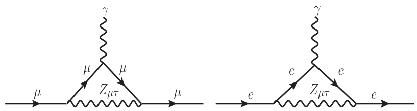
Figure 1: Feynman diagrams for one loop contributions in the anomalous magnetic moments of muon and electron.

From Eq.  (17), it is clearly seen that the vectorial part and the axial vectorial part of the interaction between $Z_{\mu\tau}$ and leptons act oppositely (true for any gauge boson) in the anomalous magnetic moment and the net effect due to a new gauge boson is the difference between the contributions of both interactions. In the limit of small kinetic mixing ($\epsilon\rightarrow 0$), $\Delta{a}_{e}$ goes to zero while $\Delta{a}_{\mu}\propto g^{2}_{\mu\tau}$, gets contribution from the vectorial part only.

The recent measurement of $(g-2)_{\mu}$ shows a $4.2\sigma$ deviation from the SM prediction with a magnitude of $\Delta{a}_{\mu}=a^{exp}_{\mu}-a^{SM}_{\mu}=(2.51\pm 0.59)\times 10^{-9}$ Muong-2:2021ojo . On the other hand, there are two existing values of $\Delta{a}_{e}$ due to two different measurements of the fine structure constant ($\alpha_{em}$) at Berkeley with ${}^{137}{\rm Cs}$ atom Parker:2018vye and LKB with ${}^{87}{\rm Rb}$ atom Morel:2020dww respectively. Using these measurements, the SM prediction for $a_{e}\equiv\dfrac{(g-2)_{e}}{2}$ is either higher ($2.4\sigma$ deviation) or lower ($1.6\sigma$ deviation) than the experiment value Hanneke:2008tm . More importantly, the nature of new physics is determined by the measurement of $\alpha_{em}$, where the former case requires a destructive BSM contribution while an opposite situation is need for the latter. In the case of muon we always need a positive contribution to $a_{\mu}$ from the BSM theory as the SM prediction is lower than the experimental measurement. Therefore, depending upon the value of $\alpha_{em}$, we either need positive values of $\Delta{a_{\ell}}$ for both $e$ and $\mu$ or we require a positive $\Delta{a_{\mu}}$ along with a negative $\Delta{a_{e}}$. Although, there is a relative sign difference between the contributions coming from the vectorial and the axial vectorial parts of the interaction to $\Delta{a}_{\ell}$ as seen from Eq. (17), it is not possible to achieve the second possibility in the minimal $L_{\mu}-L_{\tau}$ model. The reason behind this is that for muon we need dominance of the vectorial part of interaction while for $e$ the axial vectorial dominance, which mainly comes from tiny $Z-Z_{\mu\tau}$ mixing, is required. On the other hand, the first possibility where we need same sign of $\Delta{a_{\ell}}$ can be achieved easily in the minimal model. However, the parameter space addressing both the experimental values for $\Delta{a_{\mu}}=(2.51\pm 0.59)\times 10^{-9}$ and $\Delta{a_{e}}=(4.8\pm 3.0)\times 10^{-13}$ is already excluded by the measurement of $\nu_{e}\,e$ scattering at Borexino experiment. In Fig.  2 we have summarised all results in the familiar $g_{\mu\tau}-M_{Z_{\mu\tau}}$ plane.

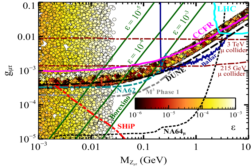
Figure 2: Parameter space for $(g-2)_{e}$ (circular points) and $(g-2)_{\mu}$ (plus shaped points) with relevant experimental constraints in $g_{\mu\tau}-M_{Z_{\mu\tau}}$ plane. Solid lines represent existing bounds while other lines are projected exclusion limits from future experiments.

In this figure, the $2\sigma$ contour of $(g-2)_{\mu}$ has been shown by plus shaped points while the corresponding contour for $(g-2)_{e}$ is denoted by circular points. The colour-bar indicates variation of the kinetic mixing parameter in the following range $10^{-6}\leq\epsilon\leq 10^{-3}.$ It is clearly seen that to obtain a sufficient contribution in $\Delta{a_{e}}$ from $Z_{\mu\tau}$ we need $\epsilon\gtrsim 10^{-4}$ while for $\mu$, the parameter $\epsilon$ can be as low as $10^{-6}$ or even smaller. This is mainly due to the fact that the interaction of $e^{+}\,e^{-}$ with $Z_{\mu\tau}$ is entirely governed by the $Z-Z_{\mu\tau}$ mixing since $e^{\pm}$ do not have any $L_{\mu}-L_{\tau}$ charge. However, the vectorial part of interaction for $\mu^{\pm}$, responsible for getting a positive $\Delta{a_{\mu}}$, is dominated by a factor proportional to the $L_{\mu}-L_{\tau}$ charge. The overlapping region in Fig. 2 satisfies both the experimental values of anomalous magnetic moments and the corresponding parameters are $3\times 10^{-4}\lesssim g_{\mu\tau}\lesssim 10^{-3}$, $M_{Z_{\mu\tau}}\lesssim 0.3$ GeV and $\epsilon\gtrsim 10^{-4}$. However, as one can see from Fig. 2 that the above parameter space for $\epsilon\gtrsim 10^{-4}$ is already ruled-out from the observation of $e-\nu$ scatterings at Borexino experiment. We have depicted excluded regions in $g_{\mu\tau}-M_{Z_{\mu\tau}}$ plane for three different values of the kinetic mixing parameters for which the $e-\nu$ scattering cross section in the minimal $L_{\mu}-L_{\tau}$ model lies outside the $2\sigma$ range obtained from Borexino experiment i.e. $0.88<\dfrac{\sigma^{L_{\mu}-L_{\tau}}_{e\nu}}{\sigma^{\rm SM}_{e\nu}}<1.24$ Borexino:2017rsf ; Altmannshofer:2019zhy . The other relevant existing/proposed experimental bounds from CCFR, DUNE using neutrino tridents ($\nu_{\mu}N\rightarrow\nu_{\mu}N\mu^{+}\mu^{-}$) Altmannshofer:2014pba and also from four $\mu$ production at LHC ($p\,p\rightarrow Z_{\mu\tau}\mu^{+}\mu^{-}\rightarrow\mu^{+}\mu^{-}\mu^{+}\mu^{-}$) CMS:2018yxg , BaBar ($e^{+}\,e^{-}\rightarrow Z_{\mu\tau}\mu^{+}\mu^{-}\rightarrow\mu^{+}\mu^{-}\mu^{+}\mu^{-}$) BaBar:2016sci are also shown in Fig. 2. Additionally, projected bounds from the proposed muon collider MuonCollider:2022xlm for two different centre of mass energies are also presented in the $g_{\mu\tau}-M_{Z_{\mu\tau}}$ plane, where the corresponding bounds are obtained from a combination of $Z_{\mu\tau}$+$\gamma$ searches and from variation in angular observables of the Bhabha scattering. Moreover, proposed exclusion limits in the $g_{\mu\tau}-M_{Z_{\mu\tau}}$ plane from different beam-dump experiments namely, Na62 (from charged kaon decays, $K\rightarrow\mu\nu Z_{\mu\tau}\rightarrow\nu\mu\,\nu\bar{\nu}$) Krnjaic:2019rsv , Na64_μ (from large missing energy of muon beam due to bremsstrahlung of muons in presence of target nuclei and subsequent invisible decay of $Z_{\mu}\rightarrow\nu\bar{\nu}$) Gninenko:2014pea , SHiP SHiP:2015vad etc. are included to indicate the future detection prospects of the $L_{\mu}-L_{\tau}$ scenario. Finally, for completeness, we have also demonstrated the proposed sensitivity region from a new muon missing momentum experiment M³ at Fermi lab Kahn:2018cqs . Therefore, it is quiet evident that there are lots of experimental efforts to detect a possible light $Z_{\mu\tau}$ and within a next few years the entire $g_{\mu\tau}-M_{Z_{\mu\tau}}$ parameter space that satisfies $(g-2)_{\mu}$ in $2\sigma$ range will be probed.

III Extended $L_{\mu}-L_{\tau}$ Model

In the previous section, we have tried to expound both the anomalies reported in $g-2$ of muon and electron in a common framework. While doing so we have noticed that the minimal model is not sufficient and we need some extension of the minimal model. Moreover, we would also like to see that the extended model is good enough to address issues related to neutrino mass and dark matter. Therefore, in order to accomplish these unresolved issues, we extend particle contents of the minimal $L_{\mu}-L_{\tau}$ model. In particular, we introduce a vector like fermion $\chi$ with nonzero U(1)_Y and U(1)${}_{L_{\mu}-L_{\tau}}$ quantum numbers and has no colour and weak-isospin charges. Additionally, in the fermionic sector we include three right handed neutrinos, having transformation properties similar to the SM leptons under U(1)${}_{L_{\mu}-L_{\tau}}$, for neutrino mass generation via Type-I seesaw mechanism. In the scalar sector, besides the SM Higgs doublet $\Phi^{\prime}_{1}$ and previously introduced $L_{\mu}-L_{\tau}$ breaking scalar $\Phi^{\prime}_{3}$, we have one SU(2)_L doublet $\Phi^{\prime}_{2}$ and a SU(2)_L singlet $\Phi^{\prime}_{4}$ with suitable $L_{\mu}-L_{\tau}$ charges to construct new Yukawa interactions between the SM Leptons and $\chi$. As we will see later, both these scalars along with the charged fermion $\chi$ have played a pivotal role in generating $(g-2)_{e}$ in the ballpark of experimental measurements. In Tables (2, 3), we have shown the complete particle spectrum and associated charges under the complete gauge group $SU(3)_{C}\times SU(2)_{L}\times U(1)_{Y}\times U(1)_{L_{\mu}-L_{\tau}}$ of the present model. Here we would like to note that since all fermions are vector like under the $L_{\mu}-L_{\tau}$ symmetry the extended model is also anomaly free as it was for the minimal model.

Gauge Group ${\rm SU(2)}_{\rm L}$ ${\rm U(1)}_{\rm Y}$

Baryon Fields $Q_{L}^{i}=(u_{L}^{i},d_{L}^{i})^{T}$ $u_{R}^{i}$ $d_{R}^{i}$ $2$ $1$ $1$ $1/6$ $2/3$ $-1/3$

Lepton Fields $L_{L}^{i}=(\nu_{L}^{i},e_{L}^{i})^{T}$ $e_{R}^{i}$ $N_{R}^{i}$ $\chi_{{}_{L}}$ $\chi_{{}_{R}}$ $2$ $1$ $1$ $1$ $1$ $-1/2$ $-1$ $0$ $-1$ $-1$

Scalar Fields $\Phi^{\prime}_{1}$ $\Phi^{\prime}_{2}$ $\Phi^{\prime}_{3}$ $\Phi^{\prime}_{4}$ $2$ $2$ $1$ $1$ $1/2$ $1/2$ $0$ $0$

Table 2: Particle contents and their corresponding charges under the SM gauge group.

Gauge Group ${\rm U(1)}_{L_{\mu}-L_{\tau}}$

Baryonic Fields $(Q^{i}_{L},u^{i}_{R},d^{i}_{R})$ $0$

Lepton Fields $(L_{L}^{e},e_{R},N_{R}^{e})$ $(L_{L}^{\mu},\mu_{R},N_{R}^{\mu})$ $(L_{L}^{\tau},\tau_{R},N_{R}^{\tau})$ $\chi_{{}_{L}}$ $\chi_{{}_{R}}$ $0$ $1$ $-1$ $1/3$ $1/3$

Scalar Fields $\Phi^{\prime}_{1}$ $\Phi^{\prime}_{2}$ $\Phi^{\prime}_{3}$ $\Phi^{\prime}_{4}$ $0$ $-1/3$ $1$ $-1/3$

Table 3: $L_{\mu}-L_{\tau}$ charges for fermions and scalars of the present model.

The full Lagrangian of the present model is given by

$$\mathcal{L}=\mathcal{L}_{\rm SM}-\frac{1}{4}\hat{X}_{\alpha\beta}\hat{X}^{\alpha\beta}+\frac{\epsilon}{2}\hat{X}_{\alpha\beta}\hat{B}^{\alpha\beta}-g_{\mu\tau}\sum_{\begin{subarray}{c}\ell=\mu,\nu_{\mu},\\ \,\,\,\tau,\nu_{\tau}\end{subarray}}Q^{\ell}_{\mu\tau}\bar{\ell}\gamma^{\alpha}\ell\hat{X}_{\alpha}+\bigg{[}i\,\bar{\chi}\not{\partial}\chi-\bar{\chi}\gamma^{\alpha}\chi\left(\dfrac{g_{\mu\tau}}{3}\hat{X}_{\alpha}-{g_{1}}\hat{B}_{\alpha}\right)$$

$$-M_{\chi}\overline{\chi}\chi-\biggl{(}\beta^{R}_{e\chi}\overline{L_{e}}\Phi^{\prime}_{2}\chi_{{}_{R}}+\beta^{L}_{e\chi}\overline{e_{R}}\,\chi_{{}_{L}}\Phi^{\prime}_{4}+{\it h.c.}\biggr{)}\bigg{]}+\mathcal{L}_{N}+\sum_{i=2}^{4}\left(D_{\alpha}{\Phi^{\prime}_{i}}\right)^{\dagger}\left(D^{\alpha}{\Phi^{\prime}_{i}}\right)-\mathcal{V}(\Phi^{\prime}_{1},\Phi^{\prime}_{2},\Phi^{\prime}_{3},\Phi^{\prime}_{4})\,.$$

(22)

Apart from the terms which have already defined in the previous section, the terms within the square brackets represent the Lagrangian of vector like fermion $\chi$ including the new Yukawa interactions with couplings $\beta^{R}_{e\chi}$ and $\beta^{L}_{e\chi}$ respectively. The Lagrangian for three right handed neutrinos are denoted by $\mathcal{L}_{N}$. We have written the exact form of $\mathcal{L}_{N}$ below.

$$\mathcal{L}_{N} = \frac{i}{2}\sum_{\begin{subarray}{c}i=e,\mu,\\ \tau\end{subarray}}\overline{N_{i}}\not{D}N_{i}+\sum_{\begin{subarray}{c}i=e,\mu,\\ \tau\end{subarray}}\big{(}y_{ii}\,\overline{L_{i}}\Phi^{\prime}_{1}N_{i}+{\it h.c.}\big{)}+\big{(}M_{ee}N_{e}N_{e}+h_{e\mu}N_{e}N_{\mu}{\Phi^{\prime}_{3}}^{\dagger}$$ (23)

$$+h_{e\tau}N_{e}N_{\tau}\Phi^{\prime}_{3}+M_{\mu\tau}e^{i\theta}N_{\mu}N_{\tau}+{\it h.c.}\big{)}\,,$$

where, the first term is the kinetic term of $N_{i}$ while the rest are interaction terms responsible for the light neutrino mass generation via Type-I seesaw mechanism. We refrain further discussion on this topic and will discuss again when we talk about neutrino mass in Section IV. Finally, the last two terms in Eq. (22) are the kinetic and interaction terms for the BSM scalars ($\Phi^{\prime}_{i},\,i=2,\,3,\,4$). In the kinetic term, $D_{\alpha}$ being the usual covariant derivative involving gauge boson(s) and generator(s) of each group under which $\Phi^{\prime}_{i}$ transforms non-trivially. The explicit form of $\mathcal{V}$, invariant under the full gauge group, is given below

$$\mathcal{V}(\Phi^{\prime}_{1},\Phi^{\prime}_{2},\Phi^{\prime}_{3},\Phi^{\prime}_{4}) = \sum^{4}_{i=2}\left[\mu^{2}_{i}\left({\Phi^{\prime}}^{\dagger}_{i}\Phi^{\prime}_{i}\right)+\lambda_{i}\left({\Phi^{\prime}}^{\dagger}_{i}\Phi^{\prime}_{i}\right)^{2}\right]+\sum_{i,j,j>i}\lambda_{ij}\left({\Phi^{\prime}}^{\dagger}_{i}\Phi^{\prime}_{i}\right)\left({\Phi^{\prime}}^{\dagger}_{j}\Phi^{\prime}_{j}\right)$$ (24)

$$+\lambda^{\prime}_{12}\left({\Phi^{\prime}}^{\dagger}_{1}\Phi^{\prime}_{2}\right)\left({\Phi^{\prime}}^{\dagger}_{2}\Phi^{\prime}_{1}\right)+\left[\mu\left({\Phi^{\prime}_{1}}^{\dagger}\Phi^{\prime}_{2}\right){\Phi^{\prime}_{4}}^{\dagger}+\xi\left(\Phi^{\prime}_{3}{\Phi^{\prime}_{4}}^{3}\right)+{\it h.c.}\right].$$

Here for necessary vacuum alignment we need $\mu^{2}_{1,3}<0$, $\mu^{2}_{2,4}>0$ and $\lambda_{i}>0$. The second condition, $\mu^{2}_{2,4}>0$, ensures that two new $L_{\mu}-L_{\tau}$ charged scalars $\Phi^{\prime}_{2}$ and $\Phi^{\prime}_{4}$ do not have any VEV. Apart from the usual self-conjugate terms, we have two non-self-conjugate terms also in the Lagrangian which have utmost importance in the present context. The trilinear term with coefficient $\mu$ introduces mixing between the neutral component of $\Phi^{\prime}_{2}$ and $\Phi^{\prime}_{4}$. Since the VEVs of both these scalars are zero, the lightest one is automatically stable and can be a viable dark matter candidate. Therefore, for a singlet like dark matter candidate (dominated by $\Phi^{\prime}_{4}$), which is precisely the case we are considering, this mixing opens up a direct detection prospect through exchange of the SM $Z$ boson. On the other hand, the quartic term proportional to $\xi$ is responsible for cubic interaction among the dark matter particles, which results in some higher order number changing processes ($3\rightarrow 2$). After both EWSB and $L_{\mu}-L_{\tau}$ breaking, the $2\times 2$ mass matrix for the neutral component of $\Phi^{\prime}_{2}$ ($\phi^{\prime}_{2}$) and $\Phi^{\prime}_{4}$ is given by

$$M^{2}_{\phi^{\prime}_{2}-\Phi^{\prime}_{4}}=\begin{pmatrix}a&b\\ b&c\end{pmatrix}\,.$$ (25)

where $a=\mu^{2}_{2}+(\lambda_{12}+\lambda^{\prime}_{12})\frac{v^{2}}{2}+\lambda_{23}\frac{v_{\mu\tau}}{2}$, $c=\mu^{2}_{4}+\lambda_{14}\frac{v^{2}}{2}+\lambda_{34}\frac{v_{\mu\tau}}{2}$ and $b=\frac{\mu v}{\sqrt{2}}$. One can easily diagonalise the above mass matrix using an orthogonal transformation by an angle $\theta_{D}$ and the resultant eigenstates are related to the old basis sates $(\phi^{\prime}_{2},\,\,\Phi^{\prime}_{4})$ in the following way

$$\begin{pmatrix}\phi_{2}\\ \phi_{4}\end{pmatrix}=\begin{pmatrix}\cos\theta_{D}&-\sin\theta_{D}\\ \sin\theta_{D}&\cos\theta_{D}\end{pmatrix}\,\,\begin{pmatrix}\phi^{\prime}_{2}\\ \Phi^{\prime}_{4}\end{pmatrix}\,,$$ (26)

where, the mixing angle $\theta_{D}$ can be expressed in terms of the parameters of the Lagrangian as,

$$\theta_{D} = \dfrac{1}{2}\tan^{-1}\left(\dfrac{2b}{c-a}\right)\,,$$ (27)

$$= \dfrac{1}{2}\tan^{-1}\left[\dfrac{\sqrt{2}\,{\mu v}}{\mu^{2}_{4}-\mu^{2}_{2}+(\lambda_{14}-\lambda_{12}-\lambda^{\prime}_{12})\frac{v^{2}}{2}+(\lambda_{34}-\lambda_{23})\frac{v_{\mu\tau}}{2}}\right]$$

and the masses corresponding to the physical states $\phi_{2}$ and $\phi_{4}$ are

$$M^{2}_{\phi_{2}} = \left[\mu^{2}_{2}+(\lambda_{12}+\lambda^{\prime}_{12})\frac{v^{2}}{2}+\lambda_{23}\frac{v_{\mu\tau}}{2}\right]\cos^{2}\theta_{D}+\left[\mu^{2}_{4}+\lambda_{14}\frac{v^{2}}{2}+\lambda_{34}\frac{v_{\mu\tau}}{2}\right]\sin^{2}\theta_{D}-\frac{\mu v}{\sqrt{2}}\sin 2\theta_{D}\,,$$

$$M^{2}_{\phi_{4}} = \left[\mu^{2}_{2}+(\lambda_{12}+\lambda^{\prime}_{12})\frac{v^{2}}{2}+\lambda_{23}\frac{v_{\mu\tau}}{2}\right]\sin^{2}\theta_{D}+\left[\mu^{2}_{4}+\lambda_{14}\frac{v^{2}}{2}+\lambda_{34}\frac{v_{\mu\tau}}{2}\right]\cos^{2}\theta_{D}+\frac{\mu v}{\sqrt{2}}\sin 2\theta_{D}\,.$$

In our work, we have considered that $\phi_{4}$ is the lightest state and is a suitable for dark matter candidate. Similar to the $\phi^{\prime}_{2}-\Phi^{\prime}_{4}$ mixing, there is another mass mixing between the CP even neutral components $(\phi^{\prime}_{1},\,\,\phi^{\prime}_{3})$ of the Higgs doublet $\Phi^{\prime}_{1}$ and the $L_{\mu}-L_{\tau}$ breaking scalar $\Phi^{\prime}_{3}$ respectively. This mixing is due to the presence of a quartic interaction term with coefficient $\lambda_{13}$. Therefore, after spontaneous symmetry breaking this quartic interaction generates off-diagonal terms in the $2\times 2$ mass matrix which is given by

$$M^{2}_{\phi^{\prime}_{1}-\phi^{\prime}_{3}}=\begin{pmatrix}2\lambda_{1}v^{2}&\lambda_{13}vv_{\mu\tau}\\ \lambda_{13}vv_{\mu\tau}&2\lambda_{3}v^{2}_{\mu\tau}\end{pmatrix}\,.$$ (29)

This symmetric mass matrix can be diagonalised in a similar manner as above and as a result, we get two physical states $h_{1}$ and $h_{3}$ with a mixing angle $\theta$ which can be expressed as,

$$\theta=\dfrac{1}{2}\tan^{-1}\left[\frac{\lambda_{13}vv_{\mu\tau}}{\lambda_{3}v_{\mu\tau}^{2}-\lambda^{2}_{1}v^{2}}\right].$$ (30)

In this work we have considered $h_{1}$ as the SM like Higgs boson which was discovered by the ATLAS ATLAS:2012yve and the CMS CMS:2012qbp collaborations in 2012 and having mass $M_{h_{1}}=125.5$ GeV. We would like to mention in passing that the CP odd neutral components of $\Phi^{\prime}_{1}$ and $\Phi^{\prime}_{3}$ turn into the Goldstone bosons after both $Z$ and $Z_{\mu\tau}$ become massive. Therefore, in the scalar sector of the extended model, apart from the SM like Higgs boson $h_{1}$, we have one CP even scalar ($h_{2}$), one charged scalar (part of the doublet $\Phi^{\prime}_{2}$) and two complex scalars ($\phi_{2}$, $\phi_{4}$). The latter take part in one loop diagram contributing to $(g-2)_{e}$ while $\phi_{4}$ plays the role of dark matter with enhanced detection possibilities directly due to $\phi_{2}$. As mentioned in the previous section, besides the contribution coming from $Z_{\mu\tau}$ through kinetic mixing, the new Yukawa interactions (defined in Eq. (22) involving $e$, $\chi$ and $\phi_{i}$ ($i=2,\,4$) provide additional contribution to $(g-2)_{e}$. The details about $(g-2)_{e}$ have been discussed in Appendix A. In Fig. 15, we have shown the allowed parameter space in $\beta^{L}_{e\chi}-M_{\chi}$ plane after demanding $\Delta{a}_{e}$ in $2\sigma$ range of experimental measurement. Moreover, for the same parameter space we have also shown the $3\sigma$ and $5\sigma$ statistical significance of the charged fermion at the $e^{+}e^{-}$ linear collider.

IV Neutrino mass

As described in Eq. (23), the Lagrangian associated with the right handed neutrinos generate light neutrino masses by the Type-I seesaw mechanism Minkowski:1977sc ; Yanagida:1979as ; Mohapatra:1979ia ; Schechter:1980gr . A similar technique for generating neutrino masses in the context of ${\rm U(1)}_{L_{\mu}-L_{\tau}}$ symmetry has already been explored in detail by the present authors in Biswas:2016yan . We get both Dirac and Majorana masses when the SM Higgs doublet $\Phi^{\prime}_{1}$ and the singlet scalar $\Phi^{\prime}_{3}$ acquire VEVs. The Dirac mass matrix $M_{D}$ has the following form once the electroweak symmetry breaks,

$$M_{D}=\left(\begin{array}[]{ccc}\frac{y_{ee}v}{\sqrt{2}}{}{}&~{}~{}0{}{}&~{}~{}0\\ {}{}\hfil&{}{}\hfil\\ 0{}{}&~{}~{}\frac{y_{\mu\mu}v}{\sqrt{2}}{}{}&~{}~{}0\\ {}{}\hfil&{}{}\hfil\\ 0{}{}&~{}~{}0{}{}&~{}~{}\frac{y_{\tau\tau}v}{\sqrt{2}}\\ \end{array}\right)\,,$$ (36)

and the Majorana mass matrix $M_{R}$ takes the following form when ${\rm U(1)}_{L_{\mu}-L_{\tau}}$ symmetry gets broken,

$$\mathcal{M}_{N}=\left(\begin{array}[]{ccc}M_{ee}{}{}&~{}~{}\dfrac{v_{\mu\tau}}{\sqrt{2}}h_{e\mu}{}{}&~{}~{}\dfrac{v_{\mu\tau}}{\sqrt{2}}h_{e\tau}\\ {}{}\hfil&{}{}\hfil\\ \dfrac{v_{\mu\tau}}{\sqrt{2}}h_{e\mu}{}{}&~{}~{}0{}{}&~{}~{}M_{\mu\tau}\,e^{i\xi}\\ {}{}\hfil&{}{}\hfil\\ \dfrac{v_{\mu\tau}}{\sqrt{2}}h_{e\tau}{}{}&~{}~{}M_{\mu\tau}\,e^{i\xi}{}{}&~{}~{}0\\ \end{array}\right)\,.$$ (42)

In the Dirac mass matrix, we can rotate away the phases by redefining the left handed neutrinos on the other hand we cannot get rid of all the phases associated with the Majorana mass matrix and one phase remains which we have considered in (2,3) position. We can write down the neutrino mass matrix in the basis $({\nu_{L}}_{\alpha},{N_{R}}^{c}_{\alpha})$ ($\alpha=e,\mu,\tau$) as follows,

$$M_{\nu}=\begin{pmatrix}0&M_{D}\\ M^{T}_{D}&M_{N}\end{pmatrix}\,.$$ (43)

As demanded by the oscillation experiments and cosmology, we have the following allowed range of the oscillation parameters,

• bound on the sum of all three light neutrinos from cosmology, $\sum_{i}m_{i}<0.23$ eV at $2\sigma$ C.L. Ade:2015xua ,

• $2\sigma$ range of mass squared differences, $7.20<\dfrac{\Delta m^{2}_{21}}{10^{-5}}\,{\text{eV}^{2}}<7.94$ and
  $2.44(2.34)<\dfrac{\Delta m^{2}_{31}}{10^{-3}}\,{\text{eV}^{2}}<2.57(2.47)$ for NO(IO) deSalas:2017kay ,

• $2\sigma$ bound on the mixing angles $32.5^{\circ}<\,\theta_{12}\,<36.8^{\circ}$, $43.1^{\circ}(44.5^{\circ})<\,\theta_{23}\,<49.8^{\circ}(48.9^{\circ})$ and $8.2^{\circ}(8.3^{\circ})<\,\theta_{13}\,<8.8^{\circ}$ for NO(IO) deSalas:2017kay .

Moreover, we also have the bound on the effective number of relativistic d.o.f ($N_{eff}$) allowed from cosmology which is $N_{eff}=2.99\pm 0.17$ Planck:2018vyg . Therefore, to be consistent with all these observations and experimental measurements we can have three neutrinos in the sub-eV scale and other three are in the higher scale. This is indeed possible if we go to the seesaw regime where $M_{N}\gg M_{D}$. Then we can diagonalize the $M_{\nu}$ matrix as follows,

$$m^{light}_{\nu}\simeq-M^{T}_{D}M^{-1}_{N}M_{D}\,,\,\,\,{\rm and}\,\,\,m^{heavy}_{N}\simeq M_{N}$$ (44)

where $m^{light}_{\nu}$ corresponds to three sub-eV scale Majorana neutrinos while $m^{heavy}_{N}$ corresponds to three heavier Majorana neutrinos. The detailed numerical analysis and the ranges of associated parameters are given in Biswas:2016yan .

V SIMP dark matter

We have seen in Section III that there are two neutral scalars $\phi_{2}$, $\phi_{4}$. The $L_{\mu}-L_{\tau}$ charge assignment (see Table 3) among the scalar fields is extremely crucial not only to get a stable dark matter candidate but also it dictates the nature of dark matter As a result, the lightest scalar $\phi_{4}$ is naturally stable and has a cubic self-interaction term when $\Phi^{\prime}_{3}$ gets a VEV. The latter is responsible for number changing interactions occurring through higher order scattering like $3\rightarrow 2$ processes. When the coupling $\xi$ of the cubic term is large enough so that the main number changing processes are $3\rightarrow 2$ scatterings rather than the usual $2\rightarrow 2$ pair annihilations of dark matter into the SM fields, the freeze-out of $\phi_{4}$ is primarily determined by the condition $\Gamma_{3\rightarrow 2}\lesssim\mathcal{H}$. Moreover, the dark matter $\phi_{4}$ maintains kinetic equilibrium with the SM bath by virtue of elastic scattering with $Z_{\mu\tau}$ where the latter remains thermally connected with the SM leptons. This is known as the SIMP paradigm Carlson:1992fn ; Hochberg:2014dra . In this work, we have explored the phenomenology of SIMP dark matter in the context of U(1)${}_{L_{\mu}-L_{\tau}}$ gauge extension. The Boltzmann equation expressing the evolution of comoving number density of dark matter is given by

$$\frac{dY_{\rm DM}}{dx} = \dfrac{{\rm s}^{2}}{\mathcal{H}\,x}\langle\sigma_{3\rightarrow 2}^{\rm tot}{\rm v}^{2}\rangle\,Y^{2}_{\rm DM}\left(Y_{\rm DM}-Y^{\rm eq}_{\rm DM}\right)-\dfrac{\rm s}{\mathcal{H}\,x}\langle\sigma_{2\rightarrow 2}^{\rm tot}{\rm v}\rangle\left(Y^{2}_{\rm DM}-(Y^{\rm eq}_{\rm DM})^{2}\right).$$

(45)

Where $Y_{\rm DM}$ is the total comoving number densities of both $\phi_{4}$ and $\phi^{\dagger}_{4}$ respectively while $x=M_{\phi_{4}}/T$ with $T$ being the photon temperature. Here we have assumed that there is no asymmetry between the number densities of particle and anti-particle of dark matter. The entropy density and the Hubble parameters are denoted by ${\rm s}$ and $\mathcal{H}$. The quantity $\langle\sigma_{3\rightarrow 2}^{\rm tot}{\rm v}^{2}\rangle$ is the thermal average of total scattering cross section for all relevant number changing $3\rightarrow 2$ processes for $\phi_{4}$ taking into account all symmetry factors

$$\sigma_{3\rightarrow 2}^{\rm tot}=-\dfrac{2}{3!}\,\sigma_{\phi_{4}\phi_{4}\phi_{4}\rightarrow\phi^{\dagger}_{4}\phi_{4}}-\dfrac{2}{2!}\,\sigma_{\phi^{\dagger}_{4}\phi_{4}\phi_{4}\rightarrow\phi^{\dagger}_{4}\phi^{\dagger}_{4}}+\dfrac{1}{3!}\,\sigma_{\phi^{\dagger}_{4}\phi^{\dagger}_{4}\phi^{\dagger}_{4}\rightarrow\phi^{\dagger}_{4}\phi_{4}}+\dfrac{1}{2!}\,\sigma_{\phi_{4}\phi^{\dagger}_{4}\phi^{\dagger}_{4}\rightarrow\phi_{4}\phi_{4}}\,.$$ (46)

Here, $+(-)$ represents increase(decrease) of $\phi_{4}$ due to a particular scattering, e.g.  the first term is the scattering cross section for a $3\rightarrow 2$ process like $\phi_{4}\phi_{4}\phi_{4}\rightarrow\phi_{4}\phi^{\dagger}_{4}$ which reduces the comoving number density of $\phi_{4}$ by 2 unit per scattering. Moreover, the factor $3!$ in the denominator is due to three identical particles in the initial state. As we have computed these $3\rightarrow 2$ processes in the non-relativistic limit of dark matter following Berlin:2016gtr , the thermal average $\langle\sigma_{3\rightarrow 2}^{\rm tot}{\rm v^{2}}\rangle$ is identical to $\sigma_{3\rightarrow 2}^{\rm tot}{\rm v^{2}}$. The matrix amplitude square ($|\mathcal{M}|^{2}$) for a particular $3\rightarrow 2$ process is related to $\sigma{\rm v^{2}}$, in the non-relativistic limit, as Berlin:2016gtr

$$\langle\sigma{\rm v}^{2}\rangle_{3\rightarrow 2}=\frac{\sqrt{5}}{S\times 384\pi M^{3}_{\phi_{4}}}\int_{-1}^{+1}d\cos\theta\,|\mathcal{M}_{3\rightarrow 2}|^{2}\,,$$ (47)

where initial and final state particles are either $\phi_{4}$ or $\phi_{4}^{\dagger}$ or both. The symmetry factor $S$ depends on number of identical particles in the final state. We have determined these amplitudes using CalcHEP Belyaev:2012qa while the necessary model files have been generated by the Mathematica based package FeynRules Alloul:2013bka . Relevant diagrams for the scattering $\phi_{4}\phi_{4}\phi_{4}\rightarrow\phi^{\dagger}_{4}\phi_{4}$ are shown in Fig. 3 and the Feynman diagrams for other processes can be generated easily following these diagrams. The necessary vertex factors are listed in Appendix  B.

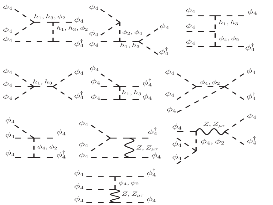
Figure 3: Feynman diagrams for the $3\rightarrow 2$ scattering $\phi_{4}\phi_{4}\phi_{4}\rightarrow\phi_{4}\phi^{\dagger}_{4}$, where comoving number density of $\phi_{4}$ decreases by 2 unit per scattering.

The second term in Eq.  (45) is coming from $2\rightarrow 2$ scatterings. These can be proceed through mediation of scalars ($h_{1}$, $h_{2}$) and gauge bosons ($Z$, $Z_{\mu\tau}$). In this work, since we want to explore the phenomenon of freeze-out within the dark sector only, we have chosen feeble scalar couplings. Therefore, the pair-annihilations of $\phi_{4}$ and $\phi^{\dagger}_{4}$ into light SM fermions are possible through exchange of $L_{\mu}-L_{\tau}$ gauge boson. Additionally, we have annihilation channel like $\phi^{\dagger}_{4}\phi_{4}\rightarrow Z_{\mu\tau}Z_{\mu\tau}$. Once we obtain these scattering cross sections using CalcHEP, the thermal average $\langle\sigma^{\rm tot}_{2\rightarrow 2}{\rm v}\rangle$ can be computed as

$$\langle\sigma^{\rm tot}_{2\rightarrow 2}{\rm v}\rangle=\dfrac{1}{4}\dfrac{1}{r^{4}_{\phi_{4}}x^{4}\,{\rm K^{2}_{2}}(r_{\phi_{4}}x)}\int_{2\,r_{\phi_{4}}x}^{\infty}dZ\,\left(\sum_{Y}\sigma_{\phi_{4}\phi^{\dagger}_{4}\rightarrow Y\overline{Y}}\right)\,Z^{2}\left(Z^{2}-4r^{2}_{\phi_{4}}x^{2}\right){\rm K_{1}}(Z)\,.$$ (48)

The sum is over all possible final states $Y$ and $Z=\dfrac{\sqrt{s}}{T}$ where $s$ is one of the Mandelstam variables. The variables $r_{\phi_{4}}=\dfrac{M_{\phi_{4}}}{M_{0}}$ and $x=\dfrac{M_{0}}{T}$ where $M_{0}$ is an arbitrary mass scale. In this work we have chosen $M_{0}=M_{\phi_{4}}$, hence $r_{\phi_{4}}=1$. We would like to note here that we need sufficient elastic scatterings between dark matter and light $L_{\mu}-L_{\tau}$ charged leptons to keep the dark sector thermally connected with the SM bath. We have discussed our numerical results later and we now discuss the relevant bounds that we have considered in the present work. These are listed below.

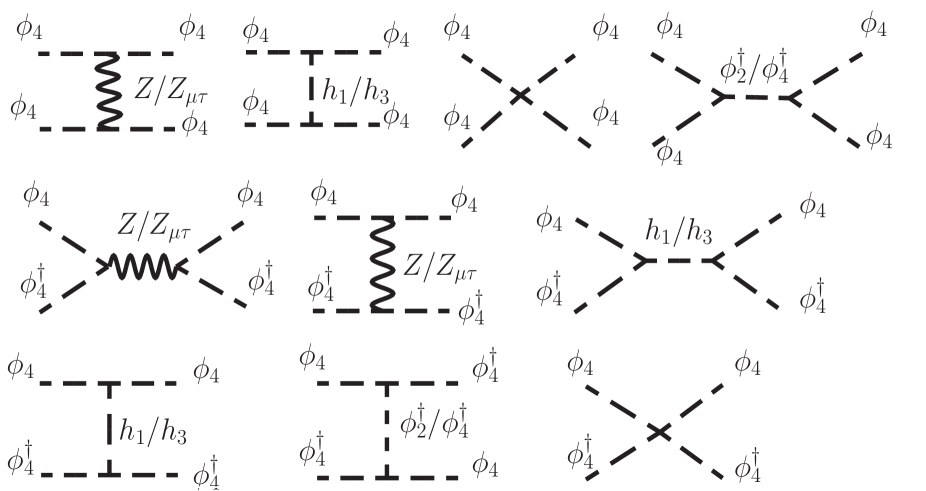
Figure 4: Feynman diagrams for the self interactions between $\phi_{4}\phi_{4}$ and $\phi_{4}\phi^{\dagger}_{4}$. The diagrams for the process $\phi^{\dagger}_{4}\phi^{\dagger}_{4}\rightarrow\phi^{\dagger}_{4}\phi^{\dagger}_{4}$ are same as those for $\phi_{4}\phi_{4}\rightarrow\phi_{4}\phi_{4}$.

• Self Interaction: Dark matter $\phi_{4}$ and $\phi^{\dagger}_{4}$ in our present model have the following self scatterings which conserve their individual numbers

  $$\phi_{4}\phi_{4}\rightarrow\phi_{4}\phi_{4}\,,\,\,\,\phi_{4}\phi^{\dagger}_{4}\rightarrow\phi_{4}\phi^{\dagger}_{4}\,,\,\,\,\phi^{\dagger}_{4}\phi^{\dagger}_{4}\rightarrow\phi^{\dagger}_{4}\phi^{\dagger}_{4}\,.$$ (49)

  The effective self interaction cross section, considering both $\phi_{4}$ and $\phi^{\dagger}_{4}$ contribute an equal amount to the relic density, is given by

  $$\sigma_{\rm self}=\dfrac{1}{4}\left(\sigma_{\phi_{4}\phi_{4}}+\sigma_{\phi_{4}\phi^{\dagger}_{4}}+\sigma_{\phi^{\dagger}_{4}\phi^{\dagger}_{4}}\right)\,.$$ (50)

  The individual scattering cross sections are obtained using the package CalcHEP and the corresponding Feynman diagrams are shown in Fig.  4. Thereafter we have enforced the non-relativistic limit by putting $s\simeq 4\,M^{2}_{\phi_{4}}+M^{2}_{\phi_{4}}\,{\rm v}^{2}$ and taking ${\rm v}\rightarrow 0$ where ${\rm v}$ is the relative velocity in the centre of mass frame. From the observation of the bullet cluster Clowe:2003tk ; Markevitch:2003at there is a bound on the ratio $\frac{\sigma_{\rm self}}{M_{\phi_{4}}}\lesssim 1\,\,{\rm cm^{2}}/{\rm g}$. The bound depends on the relative velocity of dark matter particles in a particular galaxy. Similarly, the Abell 520 cluster merger predicts $\frac{\sigma_{\rm self}}{M_{\phi_{4}}}\sim 1\,\,{\rm cm^{2}}/{\rm g}$ . Moreover, there is a wide range of the allowed values of $\frac{\sigma_{\rm self}}{M_{\phi_{4}}}$ from various astrophysical observations and N-body simulations Tulin:2017ara . To be consistent with maximum number of observations, in this work, we have considered $0.1\,\,{\rm cm^{2}/g}\leq\frac{\sigma_{\rm self}}{M_{\phi_{4}}}\leq 10\,\,{\rm cm^{2}}/{\rm g}$.

• Perturbativity and Unitarity: We have considered perturbative limit ($<4\pi$) on all the quartic couplings in Eq.  (24) so that the vacuum does not become unbounded from below for the large value of scalar fields.  Moreover, decomposing the matrix amplitude of a scattering process into partial waves, the requirement of unitarity of S-matrix demands

  $$|\mathcal{M}|\leq 16\pi\,.$$ (51)

• Direct Detection bound: The dark matter candidates $\phi_{4}$ and $\phi^{\dagger}_{4}$ in the present model can be detected at the direct detection experiments by scattering with heavy nuclei and electrons as well. Instead of being predominantly an SU(2)_L singlet like state, the mixing of $\Phi^{\prime}_{4}$ with the neutral component of inter doublet $\Phi^{\prime}_{2}$ generates $\phi_{4}\phi_{4}^{\dagger}Z$ vertex. This is a vectorial interaction (proportional to $\gamma_{\mu}$) only. On the other hand, the $\bar{f}fZ$ ($f$ is any SM fermion) vertex factor has both the vectorial as well as the axial vectorial (proportional to $\gamma_{\mu}\gamma_{5}$) parts. While the vectorial part is responsible for spin independent scattering, spin dependent scattering is possible due to the axial vectorial part. As a result, we have both spin independent as well as spin dependent scatterings when dark matter scatters off through $Z$ boson.  The spin independent elastic scattering cross sections is given by

  $$\sigma_{\rm SI} = \left(\dfrac{g_{2}\,\sin^{2}\theta_{D}}{2\,\cos\theta_{W}}\right)^{2}\dfrac{\mu^{2}_{\phi_{4}\,N}}{\pi\,M^{4}_{Z}}\times$$ (52)

  $$\left[\dfrac{\mathbb{Z}\left\{2a_{q}(\frac{1}{2},\frac{2}{3})+a_{q}(-\frac{1}{2},-\frac{1}{3})\right\}+(\mathbb{A-Z})\left\{a_{q}(\frac{1}{2},\frac{2}{3})+2a_{q}(-\frac{1}{2},-\frac{1}{3})\right\}}{\mathbb{A}}\right]^{2},$$

  where,

  $$a_{q}(T_{3},Q^{q}_{em})=-\dfrac{g}{2\,\cos\theta_{W}}\left\{\left(T_{3}-2\,Q^{q}_{em}\sin^{2}\theta_{W}\right)\cos\theta_{\mu\tau}+\epsilon\sin\theta_{W}\left(T_{3}-2\,Q^{q}_{em}\right)\sin\theta_{\mu\tau}\right\}$$

  is the vectorial part of $\bar{q}qZ$ coupling while $\mathbb{Z}$, $\mathbb{A}$ are atomic number and mass number of the detector nucleus respectively. The reduced mass between dark matter matter and nucleon $N$ is denoted by $\mu_{\phi_{4}\,N}$. The spin dependent scattering cross section is given by

  $$\sigma_{\rm SD}=\left(\dfrac{g_{2}\,\sin^{2}\theta_{D}}{2\,\cos^{2}\theta_{W}}\right)^{2}\dfrac{\mu^{2}_{\phi_{4}\,N}}{\pi\,M^{4}_{Z}}{\rm v^{2}_{lab}}\,F_{q}^{2}\,,$$ (53)

  the quantity $F_{q}$ is given by

  $$F_{q}=\dfrac{b_{q}(\frac{1}{2})\left\{\Delta^{p}_{u}\,\langle S_{p}\rangle+\Delta^{n}_{u}\,\langle S_{n}\rangle\right\}+b_{q}(-\frac{1}{2})\left\{\Delta^{p}_{d}\,\langle S_{p}\rangle+\Delta^{n}_{d}\,\langle S_{n}\rangle\right\}+b_{q}(-\frac{1}{2})\left\{\Delta^{p}_{s}\,\langle S_{p}\rangle+\Delta^{n}_{s}\,\langle S_{n}\rangle\right\}}{\langle S_{p}\rangle+\langle S_{n}\rangle}$$

  where, $\Delta^{p(n)}_{q}$ represents the spin content of quark $q$ in proton(neutron). The recent values of $\Delta$’s are $\Delta^{p}_{u}=\Delta^{n}_{d}=0.84$, $\Delta^{p}_{d}=\Delta^{n}_{u}=-0.43$ and $\Delta^{p}_{s}=\Delta^{n}_{s}=-0.09$ Cheng:2012qr . The contributions of proton and neutron to nuclear spin are denoted by $\langle S_{p}\rangle$ and $\langle S_{n}\rangle$ respectively. For ¹²⁹Xe isotope $\langle S_{p}\rangle=0.010$ and $\langle S_{n}\rangle=0.329$ XENON:2019rxp . The function $b_{q}(T_{3})=\dfrac{g_{2}}{2\,\cos\theta_{W}}\left(\cos\theta_{\mu\tau}+\epsilon\sin\theta_{W}\sin\theta_{\mu\tau}\right)T_{3}$ is the axial vectorial part of $\bar{q}qZ$ coupling and ${\rm v_{lab}}\simeq 10^{-3}$ is the local velocity of dark matter with respect to the laboratory frame. Moreover, in the present work since the dark mass range is in sub-GeV range, the elastic scatterings with electron also transfer energy efficiently 1108.5383 . As shown in Essig:2015cda , MeV scale DM can excite electron from valence band to conduction band and give rise to ionisation excitation. Therefore, our dark matter can also be detected through elastic scatterings with electron. We have calculated $\phi_{4}-e$ elastic scattering for the range of parameters we needed for the phenomenology and we have found that it is well below the current bound. The cross section for $\phi_{4}-e$ elastic scattering has the following form,

  $$\sigma_{elec} = \left(\dfrac{g_{2}\,\sin^{2}\theta_{D}}{2\,\cos\theta_{W}}\right)^{2}\dfrac{\mu^{2}_{\phi_{4}\,e}}{\pi\,M^{4}_{Z}}\left\{a^{2}_{e}(-\frac{1}{2},-1)+b^{2}_{e}(-\frac{1}{2}){\rm v^{2}_{lab}}\right\}\,,$$ (54)

  where the functions $a_{e}(T_{3},Q^{e}_{em})$ and $b_{e}(T_{3})$ are identical with $a_{q}$ and $b_{q}$ for the quarks. We can easily notice that the axial vector part (proportional to $b_{e}$) of $\bar{e}eZ$ interaction gives a velocity suppressed contribution to $\sigma_{elec}$ as in the case for spin dependent scattering with nuclei (Eq.  (53)).

• Kinetic equilibrium: In this work, although the freeze-out occurs after the chemical imbalance for $3\rightarrow 2$ scatterings is created within the dark sector, the kinetic equilibrium between the two sectors continues and it is primarily possible through elastic scatterings of dark matter with $\nu_{\mu}$ and $\nu_{\tau}$ where light gauge boson $Z_{\mu\tau}$ plays an important role.

  

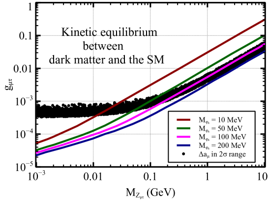
  Figure 5: The range of $g_{\mu\tau}$ and $M_{Z_{\mu\tau}}$ for which dark matter maintains kinetic equilibrium with the SM bath through elastic scatterings with $\nu_{\mu}$ and $\nu_{\tau}$ respectively.

  In Fig  5, we show the regions in $g_{\mu\tau}-M_{Z_{\mu\tau}}$ plane for four different values of $M_{\phi_{4}}$, where the kinetic equilibrium is maintained between the dark and the visible sectors. The allowed regions are the upper portions of the solid lines. For that we have used the condition $\dfrac{1}{n_{\rm scatt}}\dfrac{\Gamma_{\rm el}}{\mathcal{H}}\bigg{|}_{T\simeq M_{\phi_{4}}/20}>1$ Gorbunov:2011zz ; Gondolo:2012vh ; Biswas:2021kio , where $\Gamma_{\rm el}=\sum_{\alpha=\mu,\,\tau}n^{\rm eq}_{\nu_{\alpha}}\langle\sigma_{\phi_{4}\nu_{\alpha}\rightarrow\phi_{4}\nu_{\alpha}}{\rm v}\rangle$ is the total scattering rate per dark matter and $n_{\rm scatt}=M_{\phi_{4}}/T$ is the number of scatterings needed to transfer energy $\sim T$ between the SM bath and $\phi_{4}$. We have compared the effective interaction rate $\Gamma_{\rm el}/n_{\rm scatt}$ with the Hubble parameter ($\mathcal{H}$) around the freeze-out era of $\phi_{4}$ which is $\sim M_{\phi_{4}}/20$. For completeness, in the same $g_{\mu\tau}-M_{Z_{\mu\tau}}$ plane, we have shown the allowed parameter space satisfying $(g-2)_{\mu}$ in $2\sigma$ range by the black dots.

• Relic density bound: The abundance of dark matter has been determined quite precisely by satellite borne CMB experiments particularly the Planck experiment. The current value of dark matter relic density is Planck:2018vyg

  $$\Omega_{\rm DM}h^{2}=0.120\pm 0.001$$ (55)

• Invisible Higgs Decay: We are considering sub-GeV dark matter in the present case. As a result, the SM like Higgs boson $h_{1}$ can decay into a pair of $\phi_{4}$ and $\phi^{\dagger}_{4}$. Moreover, $h_{1}$ can decay into a pair of light gauge boson $Z_{\mu\tau}$ also. These additional decay modes contribute to the invisible decay of $h_{1}$. The LHC has placed an upper bound on the branching ratio of total invisible decay of the Higgs boson, which is CMS:2018yfx ,

  $${\rm Br}(h_{1}\rightarrow{\rm invisible\,\,channels})<0.19\,.$$ (56)

  However, the bound is easily satisfied in our model as we have considered feeble scalar portal couplings while the other decay mode $h_{1}\rightarrow Z_{\mu\tau}Z_{\mu\tau}$ is suppressed by $\sin^{4}\theta_{\mu\tau}$.

V.1 Numerical Results

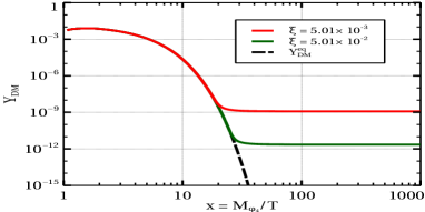
(a) $Y_{\rm DM}$ vs $x$ plot for two different values of $\xi$

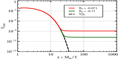
(b) $Y_{\rm DM}$ vs $x$ plot for two different values of $\theta_{D}$

(c) $Y_{\rm DM}$ vs $x$ plot for two different $M_{\phi_{2}}$

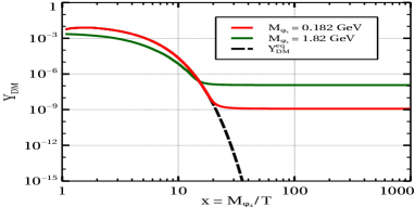
(d) $Y_{\rm DM}$ vs $x$ plot for two values of $M_{\phi_{4}}$

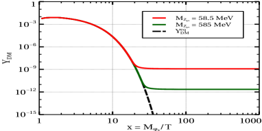
(e) $Y_{\rm DM}$ vs $x$ plot for two values of $M_{Z_{\mu\tau}}$

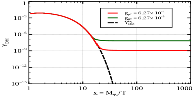
(f) $Y_{\rm DM}$ vs $x$ plot for two different values of $g_{\mu\tau}$

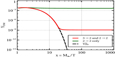
(g) Comparison on the effect of $3\rightarrow 2$ and $2\rightarrow 2$ scatterings in dark matter freeze-out

Figure 6: Numerical results: Evolution of $Y_{\rm DM}$ with $x$ for various model parameters like $\xi$, $\theta_{D}$, $M_{\phi_{2}}$, $M_{\phi_{4}}$, $M_{Z_{\mu\tau}}$ and $g_{\mu\tau}$.

In this section we have shown our results which we have obtained by solving the Boltzmann equation (Eq  (45)) numerically. The solution of Eq.  (45) is shown in Fig.  6 where we have demonstrated the evolution of $Y_{\rm DM}$ with $x$ for different model parameters. In all these plots of Fig.  6, the red solid line is the solution of the Boltzmann equation for the following set of model parameters $\xi=0.501\times 10^{-2}$, $\theta_{D}=-0.071$, $M_{\phi_{2}}=2.27$ TeV, $M_{\phi_{4}}=0.182$ GeV, $g_{\mu\tau}=6.27\times 10^{-4}$ and $M_{Z_{\mu\tau}}=58.5$ MeV, which reproduces the correct relic density. In plot (a) of Fig. 6, we have shown how the era of freeze-out and the final abundance both change when we increase $\xi$ from $0.501\times 10^{-2}$ to 0.0501 and it is indicated by the green solid line. As the $3\rightarrow 2$ scattering cross section increases with $\xi$ this results in a delayed freeze-out with a reduced final abundance. In plot (b), we have demonstrated the effect of increasing $\theta_{D}$ on $Y_{\rm DM}$. We have found that the change in mixing angle $\theta_{D}$ has a similar effect on $Y_{\rm DM}$ as it is shown in plot (a) for the parameter $\xi$. However, in this case $Y_{\rm DM}$ does not decrease as much as it is for the parameter $\xi$ for one order increase in magnitude of $\theta_{D}$.

In plot (c) we have shown the impact of $M_{\phi_{2}}$ on $Y_{\rm DM}$. Here we have increased the value of $M_{\phi_{2}}$ from $2.27$ TeV to 22.7 TeV and corresponding $Y_{\rm DM}$ has been indicated by the green solid line. Any increase in $M_{\phi_{2}}$ enhances the magnitude of cubic coupling $\mu$ as $\mu=-\dfrac{\left(M^{2}_{\phi_{2}}-M^{2}_{\phi_{4}}\right)\sin 2\theta_{D}}{\sqrt{2}v}$ with $M_{\phi_{2}}>>M_{\phi_{4}}$, which eventually increases the trilinear interaction among $\phi_{1}$, $\phi_{1}$ and $h_{1}(h_{3})$ and hence the scattering cross section $\sigma^{\rm tot}_{3\rightarrow 2}$. The effect of the mass of dark matter on $Y_{\rm DM}$ has been demonstrated in plot (d) where we have considered $M_{\phi_{4}}=0.182$ GeV (red solid line) and 1.82 GeV (green solid line) respectively. Plots (e) and (f) show the dependence of $L_{\mu}-L_{\tau}$ gauge coupling $g_{\mu\tau}$ and gauge boson mass $M_{Z_{\mu\tau}}$ on $Y_{\rm DM}$. It is seen from both the plots that any increase in $g_{\mu\tau}$ and $M_{Z_{\mu\tau}}$ has opposite effect on $Y_{\rm DM}$ respectively and it is determined by the corresponding change in $v_{\mu\tau}$ that appears in the couplings. Finally, in plot (g) we have shown the effect of $2\rightarrow 2$ and $3\rightarrow 2$ scatterings on the freeze-out of dark matter. Here the red solid line represents a situation when both $3\rightarrow 2$ as well as $2\rightarrow 2$ scatterings are present and the dark matter freezes-out around $x\simeq 20$. However, if we switch off the $3\rightarrow 2$ interactions, the freeze-out of dark matter occurs a lot earlier ($x\simeq 2$). It is due to the reason that the cross sections of $2\rightarrow 2$ scatterings are not as large as that of the $3\rightarrow 2$ scatterings which are predominantly responsible for the number changing processes.

(a) Variation of $\Omega_{\phi_{4}}h^{2}$ with $\xi$ for three different values of $M_{\phi_{4}}$.

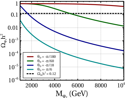
(b) Variation of $\Omega_{\phi_{4}}h^{2}$ with $M_{\phi_{4}}$ for four different values of $\theta_{D}$.

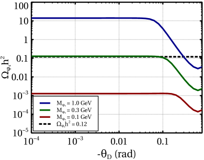
(c) $\Omega_{\phi_{4}}h^{2}$ vs $\theta_{D}$ for three different values $M_{\phi_{4}}$.

Figure 7: Variation of relic density with relevant model parameters

The variation of relic density with three most relevant parameters $\xi$, $M_{\phi_{2}}$ and $\theta_{D}$ is depicted in Fig.  7. In plot (a), dependence of $\Omega_{\phi_{4}}h^{2}$ with $\xi$ has been shown for three different values of $M_{\phi_{4}}$. Analogous to the previous plot in Fig.  6(a), here also we have noticed a similar behaviour except for $\xi<10^{-3}$, as the relic density decreases sharply with the increase of quartic coupling $\xi$ due to enhancement of $\sigma^{\rm tot}_{3\rightarrow 2}$. In plot (b), the effect of $M_{\phi_{2}}$ on $\Omega_{\phi_{4}}h^{2}$ is shown for different values of $\theta_{D}$. We can see that for low value of mixing angle ($|\theta_{D}|=\pi/180$ rad), the relic density is almost insensitive to the mass of $\phi_{2}$. However, as we increase the magnitude of $\theta_{D}$, $\Omega_{\phi_{4}}h^{2}$ decreases with $M_{\phi_{2}}$ replicating the situation shown in Fig.  6(c). The last figure in plot (c) demonstrates $\Omega_{\phi_{4}}h^{2}$ as a function of $\theta_{D}$. Here, three lines are for three different values of $M_{\phi_{4}}$ and the nature of all three lines are exactly identical to each other, i.e. the relic density is independent of the dark sector mixing angle for $|\theta_{D}|\lesssim 0.1$ rad and thereafter it starts decreasing with the increase of magnitude of $\theta_{D}$. The difference in magnitude of $\Omega_{\phi_{4}}h^{2}$ in these three lines for different $M_{\phi_{4}}$ originates from two factors. The relic density is proportional to both $M_{\phi_{4}}$ and $Y_{\rm DM}$ where the latter also gets enhanced with $M_{\phi_{4}}$ as shown in Fig.  6(d).

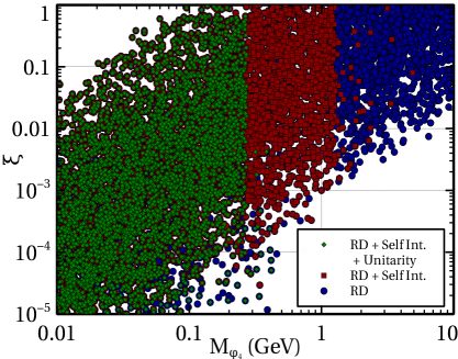
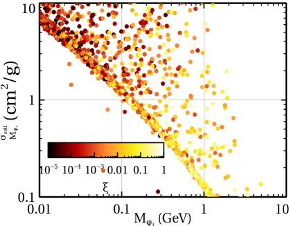
Figure 8: Left panel: Allowed parameter space is $\xi-M_{\phi_{4}}$ plane for different constraints. Right pane: Variation of $\sigma_{\rm self}/M_{\phi_{4}}$ with $M_{\phi_{4}}$.

In Fig.  8, we show our allow parameter space in $\xi-M_{\phi_{4}}$ plane. In order to obtain this we have scanned over the parameters in the following range

$$\begin{array}[]{cccccc}10^{-5}&\leq&\xi&\leq&1.0\,\,,\\ 10^{-3}\,\,{\rm rad}&\leq&|\theta_{D}|&\leq&0.1\,\,{\rm rad}\,\,,\\ 10^{-4}&\leq&g_{\mu\tau}&\leq&10^{-2}\,\,,\\ 10^{-3}\,\,{\rm GeV}&\leq&{M_{Z_{\mu\tau}}}&\leq&1.0\,\,{\rm GeV}\,\,,\\ 10^{3}\,\,{\rm GeV}&\leq&{M_{\phi_{4}}}&\leq&10^{4}\,\,{\rm GeV}\,\,,\\ 10^{-2}\,\,{\rm GeV}&\leq&{M_{\phi_{2}}}&\leq&10.0\,\,{\rm GeV}\,\,,\end{array}$$ (63)

and have imposed necessary constraints one by one. The result is shown in the left panel of Fig.  8. In this plot, the blue dots describe a region in $\xi-M_{\phi_{4}}$ plane that reproduces the correct dark matter relic density in $3\sigma$ range as determined by the Planck experiment. On top of that, we have imposed bound from dark matter self-interaction $0.1\,\,{\rm cm^{2}/g}\leq\frac{\sigma_{\rm self}}{M_{\phi_{4}}}\leq 10\,\,{\rm cm^{2}}/{\rm g}$. The resultant parameter space is indicated by the red square shaped points. Finally, we have introduced another constraint coming from the unitarity limit of scattering amplitudes as mentioned in Eq.  (51). The parameter space satisfying all three constraints is shown by the green diamond shaped points. We can notice that in order to satisfy these three constraints we need $M_{\phi_{4}}\lesssim 200$ MeV while the corresponding quartic coupling is restricted to be $\lesssim 1$. The similar result has also been presented in a different manner in the right panel of Fig.  8. Here we have shown the variation of $\sigma_{\rm self}/M_{\phi_{4}}$ with $M_{\phi_{4}}$ and the corresponding value of the parameter $\xi$ has been indicated by the colour bar. The only constraint applied in this plot is that each and every point in $\sigma_{\rm self}/M_{\phi_{4}}-M_{\phi_{4}}$ plane satisfies the relic density bound i.e. $0.117\leq\Omega_{\phi_{4}}h^{2}\leq 0.123$.

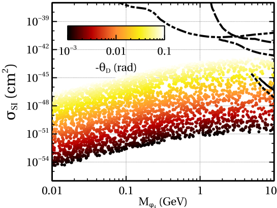
Figure 9: Spin independent scattering cross sections with exclusion limits on $\sigma_{\rm SI}$ from various ongoing as well as future experiments.

The spin independent and spin dependent elastic scattering cross sections are calculated using Eqs.  (52, 53) for the parameter range given in Eq.  (63). We have found that the spin dependent cross section is several orders of magnitude below the present bound from XENON1T XENON:2019rxp . Moreover, we also notice that $\sigma_{\rm SD}$ for a particular value of $M_{\phi_{4}}$ is almost $10^{-6}$ times smaller than the corresponding $\sigma_{\rm SI}$ and it is primarily due to the reason that $\sigma_{\rm SD}$ is suppressed by ${\rm v^{2}_{\rm lab}}$ (Eq.  (53)) where ${\rm v}_{\rm lab}\simeq 10^{-3}$ is the local velocity of dark matter particles with respect to the laboratory frame. Therefore, in Fig. 9, we have shown the spin independent scattering cross section only. In this figure, we demonstrate $\sigma_{\rm SI}$ as a function of $M_{\phi_{4}}$ and the colour bar provides the value of dark mixing angle $\theta_{D}$. Moreover, we have shown existing and future bounds from various direct detection experiments for comparison.  In the low mass region where $M_{\phi_{4}}\leq 1$ GeV, we mainly have exclusion limit on $\sigma_{\rm SI}$ from NEWS-G Durnford:2021mzg and it has been indicated by the black dashed dot dot line. The current bounds from two other low mass dark matter experiments namely, CDMSlite SuperCDMS:2017nns and DarkSide-50 DarkSide:2018bpj are shown by the dashed and the dashed dot lines respectively. The upper limit on $\sigma_{\rm SI}$ from “GeV-TeV” scale experiment like XENON1T XENON:2018voc , which has a very small overlap with our considered range of dark matter mass, has also been depicted by the black solid line. Finally, the future prediction from DARWIN DARWIN:2016hyl is shown by the dotted line.

VI Collider Signature

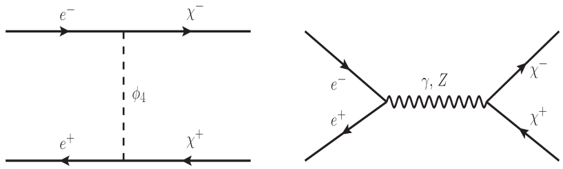
Figure 10: Charged particle production at the $e^{+}e^{-}$ collider with dark matter $\phi_{4}$ as one of the intermediate states.

In this work, we have studied the pair production of charged particles ($\chi^{+}\chi^{-}$) defined as $\chi=\chi_{L}\oplus\chi_{R}$. The produced $\chi^{\pm}$ subsequently decays into lepton and SIMP dark matter i.e. $e^{+}e^{-}\rightarrow\chi^{+}(e^{+}\phi_{4})\chi^{-}(e^{-}\phi_{4})\rightarrow e^{+}e^{-}\cancel{E}_{T}$. The Feynman diagrams contributing in the signal are mediated by $\gamma$, $Z$ and $\phi_{4}$ respectively and have been displayed in Fig.  10. We have studied the signal at two different $e^{+}e^{-}$ colliders namely, Compact Linear Collider (CLIC) CLICPhysicsWorkingGroup:2004qvu ; Dannheim:2012rn ; Linssen:2012hp ; CLICDetector:2013tfe ; CLICdp:2017vju ; Aicheler:2018arh   and International Linear Collider (ILC) Behnke:2013xla ; Adolphsen:2013kya ; Behnke:2013lya ; Baer:2013cma ; Adolphsen:2013jya . In the former case, we have considered centre of mass (c.o.m) energy $\sqrt{s}=380$ GeV and $3000$ GeV while $\sqrt{s}=500$ GeV and $1000$ GeV for the latter at the time of the pair production of vector like fermion. Depending on the c.o.m energy of the collider, we have an upper bound on the mass of $\chi^{\pm}$ upto which it can be produced. In particular, in the present work we have investigated the signal at the detector level for c.o.m energy $\sqrt{s}=1000$ GeV and $3000$ GeV of the $e^{+}e^{-}$ linear collider. Although there is no dedicated search for the present model at the CMS or ATLAS detector, still the same kind of signal can be produced at the hadron collider. We have produced the $\chi^{+}\chi^{-}$ final state at the $pp$ collider using MadGraph Alwall:2014hca ; Alwall:2011uj for $\sqrt{s}=13$ TeV and find that this is lower than the current exclusion limit given by the CMS collaboration for the 13 TeV run of LHC with 35.9 $fb^{-1}$ integrated luminosity CMS:2018xqw . This has been displayed in Fig.  11 where the red points correspond to the upper limit on the pair production cross section of the singly charged fermion coming from the study of 13 TeV run of LHC by CMS whereas the blue cross points correspond to the cross section for the present model at the $pp$ collider mediated by gauge bosons like $\gamma$ and $Z$. Therefore, we conclude that the charge particle mass range we have considered in the present model is safe from the LHC bound. In contrary to the $pp$ collider, at $e^{+}e^{-}$ collider the signal $e^{+}e^{-}\cancel{E}_{T}$ has an additional $t-$ channel diagram mediated by the MeV scale SIMP dark matter $\phi_{4}$. This $t-$channel diagram enhances the cross section by an order of magnitude larger than the $s$-channel diagrams mediated by $\gamma$ and $Z$ gauge bosons.

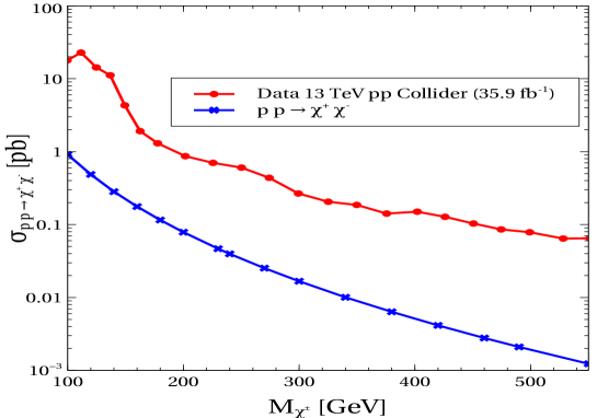
Figure 11: Production of $\chi^{+}\chi^{-}$ at the 13 TeV pp collider. Red line corresponds the bound for the production of singly charged fermion when we look for the $l^{+}l^{-}+$ MET signal at the final state. Any model which predicts the production rate above the red line is already ruled out.

In accomplishing the collider analysis for the present model, we have considered cut based analysis using a series of sophisticated packages available for the collider study. In particular, we have used FeynRules Alloul:2013bka for implementing the present model and generated the UFO model files which fed into the MadGraph Alwall:2014hca ; Alwall:2011uj subsequently. We have then used MadGraph for generating the parton level process. For showering we have used inbuilt PYTHIA Sjostrand:2006za in the MadGraph and finally for the event analysis we use DELPHES package deFavereau:2013fsa ; Selvaggi:2014mya ; Mertens:2015kba .

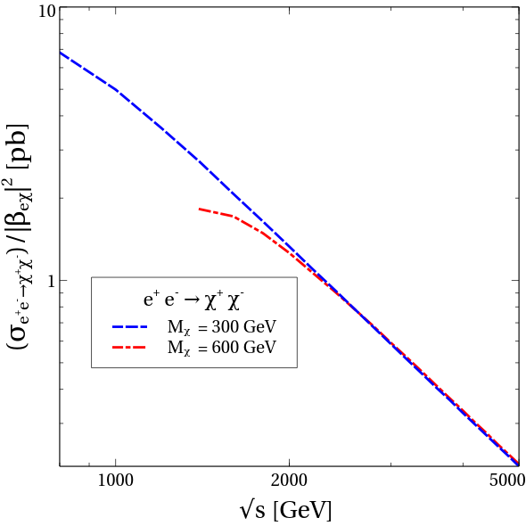
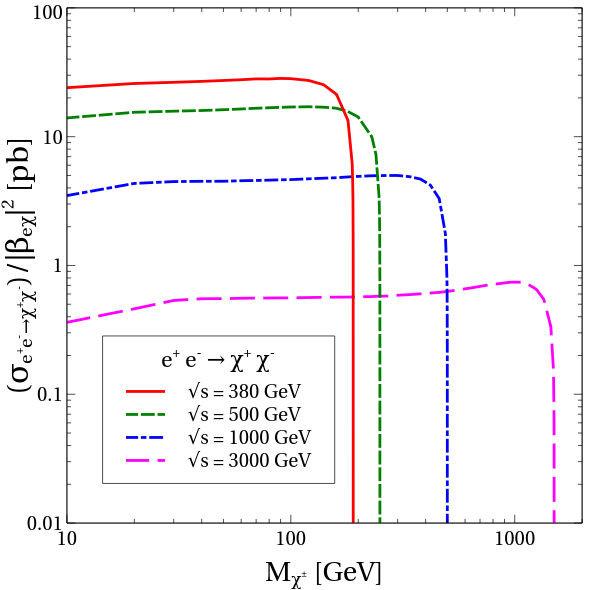
Figure 12: Left panel shows the pair production of $\chi^{+}$ and $\chi^{-}$ for different c.o.m energy for two values of $\chi^{\pm}$ mass at the $e^{+}e^{-}$ lepton collider. Right panel shows the variation of $\chi^{+}$ and $\chi^{-}$ production rate with $\chi^{\pm}$ mass $M_{\chi^{\pm}}$ for different values of c.o.m energies.

In the left and right panels of Fig. (12), we have shown the variation of $\chi^{+}\chi^{-}$ production cross section at $e^{+}e^{-}$ collider with the centre of mass energy of the collider for two different values of $\chi^{\pm}$ mass and the mass of the charged particle for the different centre of mass energies respectively. In the left panel, blue dashed line corresponds to $M_{\chi}=300$ GeV and the red dashed-dot line corresponds to $M_{\chi}=600$ GeV and both the line varies inversely with the center of mass energy $\sqrt{s}$. For $M_{\chi^{+}}=600$ GeV (red dash-dotted line), we can see that $\chi^{+}\chi^{-}$ starts producing when the c.o.m energy of the $e^{+}e^{-}$ reached a minimum threshold energy which is $\sqrt{s}=1200$ GeV. For the higher values of the c.o.m energy, we can see that blue dashed and red dashed-dot lines coincide with each other implies that the production cross section does not depend on mass for higher c.o.m values. Whereas the right panel shows the variation of $\chi^{+}\chi^{-}$ production cross section with the mass $M_{\chi^{+}}$ for different values of the c.o.m energy. One can easily see that the production cross section decrease with the increasing value of the c.o.m energy which is consistent with the discussion of the left panel. The different c.o.m energies are the proposed experimental set up for CLIC and ILC colliders. When the $\chi^{+}$ mass reached the threshold value i.e. $M_{\chi^{\pm}}\sim\frac{\sqrt{s}}{2}$, there is a sharp fall in the production cross section. In the later part of the draft, we have done the collider analysis for $\sqrt{s}=1000$ GeV and $\sqrt{s}=3000$ GeV c.o.m energy.

VI.1 Analysis

In the present work, we are interested in the signal which contains opposite sign di-electrons ($e^{+}e^{-}$) and transverse missing energy ($\cancel{E}_{T}$) in the final state. In discovering the signal from the present model, same kind of signal morphology can appear in the final state from the known SM backgrounds. The dominant backgrounds which can mimic the signal are as follows,

1. At the electron positron collider, the dominant background which can mimic the signal is $e^{+}e^{-}\rightarrow e^{+}e^{-}Z$, where $Z$ can decay to $\nu_{l}\bar{\nu}_{l}$. Therefore, finally it gives $e^{+}e^{-}\cancel{E}_{T}$ which exactly resembles the signal. This kind of background also includes $ZZ$ production channel which subsequently decays to electrons ($e^{+}e^{-}$) and neutrinos ($\nu_{l}\bar{\nu}_{l}$).

2. Another dominant background can come from the pair production of $W^{+}W^{-}$ mode at the $e^{+}e^{-}$ collider. The W-boson subsequently decays leptonically to leptons and neutrinos and can replicate the signal as $e^{+}e^{-}\rightarrow W^{+}(\rightarrow l^{+}\nu_{l})W^{-}(\rightarrow l^{-}\bar{\nu}_{l})\rightarrow e^{+}e^{-}\cancel{E}_{T}$ .

3. Another potentially relevant background is the pair production of $t\bar{t}$ mode which can also mimic the signal when $t$ quark decays leptonically associated with two b-quarks. This background can mock the signal at the electron positron collider as $e^{+}e^{-}\rightarrow t(\rightarrow b\,l^{+}\nu_{l})\bar{t}(\rightarrow\bar{b}\,l^{-}\bar{\nu}_{l})\rightarrow b\bar{b}\,e^{+}e^{-}\cancel{E}_{T}$. As we will see, this kind of signal is easy to avoid with the $b$-tagging.

At the time of generating the events, we have not put any veto to forbid the processes contains other particles than the leptons and missing energy. We can put b-veto which will reduce $t\bar{t}$ background. In Figs. (13, 14), we have shown the variation of backgrounds and signals about the different kinematical variables namely, transverse momentum of the leading electron ($P^{e_{1}}_{T}$) and second leading electron ($P^{e_{2}}_{T}$), pseudorapidity of the leading electron ($\eta_{e_{1}}$) and transverse missing energy ($\cancel{E}_{T}$). From the figures, we can choose the values of the kinematical variables which will prefer the signal over backgrounds. In this work, we have used the following kind of cuts on the kinematical variables in order to reduce the backgrounds without affecting the signal much. The details of the cuts on the kinematical variables are as follows,

1. We have considered the events which contain opposite sign di-electron ($e^{+}e^{-}$) and transverse missing energy ($\cancel{E}_{T}$). We have also put the minimal cut on the transverse momentum of the electrons which is $p^{min}_{T,e}\geq 10$ GeV. We have collected the events which satisfy the pseudorapidity of the electrons $\eta_{e}<2.5$. These cuts have been implemented at the time of the partonic generation of the events.

2. We consider events that have opposite sign di-electron pair ($e^{+}e^{-}$) in the final state.

3. From the left panel of Fig. (13), we can see that if we put strong cut on the leading electron $P^{e_{1}}_{T}\geq 130$ GeV then we can reduce the $t\bar{t}$ background. We have chosen relatively soft cut on the second leading electron which is $P^{e_{2}}_{T}\geq 60$ GeV .

4. To reduce the background which comes from $ZZ$ mode, we have used $Z-veto$. $Z-veto$ means, we have accepted the the events which violate the condition $|m_{ee}-91.2|<10$ GeV, where $m_{ee}$ is the di-electron invariant mass.

5. In order to eliminate the $t\bar{t}$ background, we have implemented $b-$veto. This implies we have rejected the events which contains $b-$quarks in the final state.

6. From the left panel of Fig. (14), we can see that background and signal peak at different values of pseudorapidity. Therefore, to reduce the background without affecting the signal much we have considered the events which have pseudorapidity in the range, $|\eta^{e}|<1.5$.

7. From the right panel of Fig. (14), we can see that if we implement a cut on the transverse missing energy then background can be reduced significantly. We have adapted the missing energy cut which is $\cancel{E}_{T}>160$ GeV.

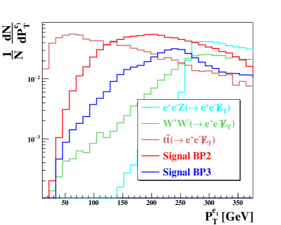
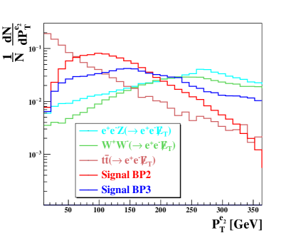
Figure 13: Left panel shows the variation of fraction of events distribution for backgrounds and signal with the transverse momentum of leading electron whereas the right panel shows the variation with respect to the rapidity of the leading electron.

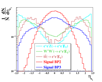
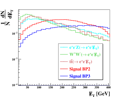
Figure 14: Variation of fraction of events for backgrounds and signal with respect to transverse missing energy and invariant mass of the di-electron in the left and right panels respectively.

SM Backgrounds at 1 TeV ILC Channels Cross section (fb) $e^{+}e^{-}Z\,(\rightarrow\nu_{l}\bar{\nu_{l}})$ $15.59$ $W^{+}(\rightarrow e^{+}\nu_{l})\,W^{-}(\rightarrow e^{-}\bar{\nu_{l}})$ $13.24$ $t(\rightarrow be^{+}\nu_{l})\,\bar{t}(\rightarrow\bar{b}e^{-}\bar{\nu_{l}})$ $1.61$ Total Backgrounds

Effective Cross section after applying cuts (fb) A0 + A1     A2      A3      A4      A5     A6 $10.07$ $6.07$ $5.88$ $5.88$ $3.92$ $2.43$ $8.88$ $6.25$ $6.25$ $6.25$ $4.28$ $1.57$ $0.73$ $0.20$ $0.20$ $0.05$ $0.04$ $0.02$ 4.02

Table 4: Cut-flow table for the obtained cross sections corresponding to the different SM backgrounds. See the text for the details of the cuts A0-A6. The c.m.energy is $\sqrt{s}=1$ TeV, relevant for ILC.

SM Backgrounds at $3$ TeV CLIC Channels Cross section (fb) $e^{+}e^{-}Z\,(\rightarrow\nu_{l}\bar{\nu_{l}})$ $6.18$ $W^{+}(\rightarrow e^{+}\nu_{l})\,W^{-}(\rightarrow e^{-}\bar{\nu_{l}})$ $1.44$ $t(\rightarrow be^{+}\nu_{l})\,\bar{t}(\rightarrow\bar{b}e^{-}\bar{\nu_{l}})$ $0.19$ Total Backgrounds

Effective Cross section after applying cuts (fb) A0 + A1     A2      A3      A4      A5     A6 $2.95$ $2.85$ $2.83$ $2.83$ $1.06$ $0.82$ $0.74$ $0.73$ $0.73$ $0.73$ $0.36$ $0.27$ $0.01$ $0.004$ $0.004$ 0.001 0.0006 0.0005 1.09

Table 5: Cut-flow table for the obtained cross sections corresponding to the SM backgrounds. The details of the cuts A0-A6 are mentioned in the text. We perform the simulation for $3$ TeV CLIC.

In Tables (4,5), we have shown the survival of the backgrounds for ILC ($\sqrt{s}=1$ TeV) and CLIC ($\sqrt{s}=3$ TeV) colliders, respectively. In Table (6), we have shown the response of the signal production cross section after applying different cuts, A0 to A6. We can see that the cuts are effective in lowering the backgrounds and at the same time cuts reduce the signal cross section less significantly than the backgrounds. In determining the statistical significance of signal over background, we have used Eq. (64). in Eq. (64), $s$ corresponds to number of events for signal after applying all the cuts and $b$ is the number of background events after applying all the cuts,

$$\mathcal{S}=\sqrt{2\times\left[(s+b){\rm ln}(1+\frac{s}{b})-s\right]}.$$ (64)

Signal at $e^{+}e^{-}$ Collider				Effective CS after cuts (fb)						Stat Significance ($\mathcal{S}$)
Experiment	Mass (GeV)	$\beta_{e\chi}$	CS (fb)	A0+A1	A2	A3	A4	A5	A6	$\mathcal{L}=1~{}{\rm fb^{-1}}$	$\mathcal{L}=10$ ${\rm fb^{-1}}$
1 TeV ILC	350.0	0.1	41.20	29.60	24.03	23.73	23.73	22.57	19.53	6.65	21.03
	450.0	0.1	29.56	21.30	19.83	19.60	19.60	19.50	17.38	6.11	19.32
3 TeV CLIC	600.0	0.1	5.13	2.91	2.78	2.78	2.78	2.16	2.05	1.60	5.04
	700.0	0.1	5.47	3.08	2.99	2.99	2.99	2.45	2.34	1.78	5.64

Table 6: Cut-flow table of signal cross section at ILC ($\sqrt{s}=1$ TeV) and CLIC ($\sqrt{s}=3$ TeV). We have considered $\beta^{L}_{e\chi}=\beta^{R}_{e\chi}=\beta_{e\chi}=0.1$ and different values of $\chi^{\pm}$ mass.

The last two columns in Table  6 corresponds to the statistical significance of the signal. For $1$ TeV collider, we can see that the present model can have more than $6\sigma$ significance for $1\,\,fb^{-1}$ luminosity. For $3$ TeV collider, we need $10\,\,fb^{-1}$ luminosity in order to get the $5\sigma$ statistical significance for the signal. We can see that the current model can be tested at the very early run of the ILC and CLIC colliders.

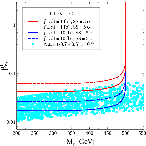
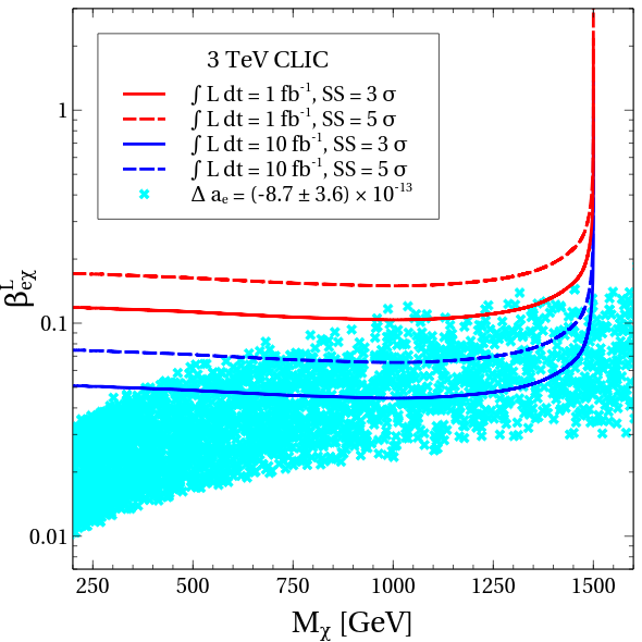
Figure 15: Left and right panels show the allowed regions (by cyan colour points) after satisfying the $(g-2)_{e}$ in $\beta^{L}_{e\chi}-M_{\chi}$ plane for 1 TeV and 3 TeV lepton colliders, respectively. The solid and dashed lines correspond to the variation of $3\sigma$ and $5\sigma$ statistical significance lines of $e^{+}e^{-}\cancel{E}_{T}$ signal with the charged singlet fermion mass for the luminosity 1 $fb^{-1}$ and 10 $fb^{-1}$, respectively. The other parameters kept fixed at $\beta^{R}_{e\chi}=\beta^{L}_{e\chi}$, $M_{\phi_{4}}=100$ MeV, $\theta_{D}=0.1$ and $M_{\phi_{2}}$ has been varied between 1 to 10 TeV.

In Fig. (15), we have shown the scatter plots in the $M_{\phi_{4}}-\beta^{L}_{e\chi}$ plane after satisfying $(g-2)_{e}$ by the cyan colour points. In the figure, the left panel corresponds to the 1 TeV ILC collider whereas the right panel is for the 3 TeV CLIC collider. The variation among the cyan colour points are due to the variation of $\phi_{2}$ mass, $M_{\phi_{2}}$, which we have considered in the range $1-10$ TeV. We have kept fixed the other parameters as mentioned in the caption of the figure. We see from both the panel that a sharp correlation between $M_{\chi}$ and $\beta^{L}_{e\chi}$ after satisfying the $(g-2)_{e}$ in the range $\Delta a_{e}=(-8.7\pm 3.6)\times 10^{-13}$. Moreover, the parameters which we have varied for $(g-2)_{e}$ also affect the production cross section of $\chi^{+}\chi^{-}$ channel at $e^{+}e^{-}$ collider. We have displayed the $1\sigma$ and $3\sigma$ statistical significance lines of the signal, $e^{+}e^{-}\rightarrow e^{+}e^{-}\cancel{E}_{T}$, by the solid and dashed lines, respectively, whereas the red and blue colors on them imply the $1\,fb^{-1}$ and $10\,fb^{-1}$ luminosity. It is easily understood from the figure that if we increased the luminosity keeping statistical significance fixed then we can access the lower values of $\beta^{L}_{e\chi}$ as well. As exhibited in the right panel of Fig. (12), the production cross section of $\chi^{+}\chi^{-}$ with the charged fermion mass, $M_{\chi}$, is flat except at the kinematical threshold limit $M_{\chi}\lesssim\frac{\sqrt{s}}{2}$ where the production cross section falls abruptly. In Table 6, we have shown the signal strength remains after applying different cuts $A0-A6$ for two benchmark points. Therefore, from the table, we can determine the average value of cut efficiency for the signal which is the ratio of the signal cross section after applying the A6 cut and the production cross section without any cuts. We find the average value of the cut efficiency for 1 TeV collider is 0.53 whereas for 3 TeV, it is 0.43. We used these values in finding the $1\sigma$ and $3\sigma$ isocontours of statistical significance for the signal in the $M_{\chi}-\beta^{L}_{e\chi}$ plane. We see that we need constant value of $\beta^{L}_{e\chi}$ for wide range of $\chi^{\pm}$ mass. Moreover, one can notice that we need higher values of $\beta^{L}_{e\chi}$ in the kinematical threshold region ($M_{\chi}\simeq\frac{\sqrt{s}}{2}$, $s$ is c.o.m energy) limit because the production cross section of $\chi^{+}\chi^{-}$ sharply falls there. Additionally, the most appealing thing to be noticed here is that we have overlap region in the $M_{\chi}-\beta^{L}_{e\chi}$ plane which gives us the correct value of $(g-2)_{e}$ and the $\geq 3\sigma$ statistical significance of the signal over background.

In order to provide an overall picture to the readers, in Table 7, we present four plausible benchmark points (BP1, BP2, BP3 and BP4) of the present model and the corresponding numerical values of several physical quantities such as dark matter relic density, direct detection cross sections, dark matter self interaction and discrepancy in leptons anomalous magnetic moment.

Parameters/	BP1	BP2	BP3	BP4
Observables
$M_{\phi_{4}}$ (GeV)	$29.216\times 10^{-3}$	$128.116\times 10^{-3}$	$168.756\times 10^{-3}$	$236.691\times 10^{-3}$
$M_{\phi_{2}}$ (GeV)	7536.32	3511.42	1282.32	3123.67
$M_{Z_{\mu\tau}}$ (GeV)	$39.405\times 10^{-3}$	$15.986\times 10^{-3}$	$124.048\times 10^{-3}$	$168.81\times 10^{-3}$
$g_{Z_{\mu\tau}}$	$6.626\times 10^{-4}$	$5.878\times 10^{-4}$	$1.003\times 10^{-3}$	$1.282\times 10^{-3}$
$\theta_{\mu\tau}$	$4.720\times 10^{-6}$	$4.720\times 10^{-6}$	$4.720\times 10^{-6}$	$4.720\times 10^{-6}$
$\theta_{D}$	$-2.347\times 10^{-2}$	$-0.815\times 10^{-2}$	$-0.1422\times 10^{-2}$	$-9.559\times 10^{-2}$
$\xi$	$0.034\times 10^{-2}$	$1.022\times 10^{-2}$	$0.343\times 10^{-2}$	$0.413\times 10^{-2}$
$\beta^{L}_{e\chi}$	0.12	0.22	0.70	0.066
$\beta^{R}_{e\chi}$	0.12	0.22	0.70	0.066
$\Omega_{\phi_{4}}h^{2}$	0.1191	0.1196	0.1199	0.1220
$\sigma_{\rm SI}$ (cm2)	$5.719\times 10^{-49}$	$1.317\times 10^{-49}$	$1.966\times 10^{-52}$	$6.958\times 10^{-45}$
$\sigma_{elec}$ (cm2)	$7.073\times 10^{-54}$	$1.057\times 10^{-55}$	$9.819\times 10^{-59}$	$1.994\times 10^{-51}$
$\sigma_{\rm SD}$ (cm2)	$2.352\times 10^{-54}$	$5.416\times 10^{-55}$	$8.085\times 10^{-58}$	$2.861\times 10^{-50}$
$\frac{\sigma_{\rm self}}{M_{\phi_{4}}}$ cm${}^{2}/$g	3.171	1.024	0.808	0.529
$\Delta{a_{\mu}}$	$2.551\times 10^{-9}$	$2.995\times 10^{-9}$	$2.213\times 10^{-9}$	$2.502\times 10^{-9}$
$\Delta{a_{e}}$	$-9.867\times 10^{-13}$	$-9.620\times 10^{-13}$	$-9.441\times 10^{-13}$	$-9.661\times 10^{-13}$

Table 7: Plausible four benchmark points (BP1, BP2, BP3 and BP4) with the numerical values of other physical quantities considered in this work.

VII Summary and conclusion

In this work, we have extended the minimal U(1)${}_{L_{\mu}-L_{\tau}}$ model by a scalar doublet ($\Phi^{\prime}_{2}$), a singlet scalar ($\Phi^{\prime}_{4}$) and a vector like singlet fermion $\chi$ to address the deviations found in experiments from the theoretical predictions of anomalous magnetic moments for both muon and electron. All these new fields have specific ${L_{\mu}-L_{\tau}}$ charges as required by the new Yukawa interactions. We have shown that in the minimal model, considering the present bounds on $Z_{\mu\tau}$ from various experiments particularly from Borexino, it is not possible to address both these anomalies simultaneously. Apart from the one loop contribution due to the neutral gauge boson $Z_{\mu\tau}$ similar to the minimal ${L_{\mu}-L_{\tau}}$ model, the additional contribution coming from one loop diagrams involving $\chi$ and $\phi_{2}$ or $\phi_{4}$ provide the deficit in $(g-2)_{e}$ as required by the experimental data when the relevant parameters remain within the following range $\beta^{L}_{e\chi}\gtrsim 5\times 10^{-2}$, $10^{-3}\,\,{\rm rad}\lesssim|\theta_{D}|\lesssim 0.1$ rad and $1\,\,{\rm TeV}\leq M_{\phi_{2}}\leq$ 10 TeV. Interestingly, in order to achieve this, we also have a natural SIMP dark matter candidate $\phi_{4}$, an admixture of $\Phi^{\prime}_{4}$ and $\phi^{\prime}_{2}$ (neutral part of $\Phi^{\prime}_{2}$), the signature of which can be found as missing energy at the upcoming $e^{+}e^{-}$ linear colliders like ILC and CLIC. In order to explore the dynamics of dark matter in detail we have considered all possible theoretical and experimental constraints arising from dark matter self interaction, perturbativity and unitarity, spin dependent and spin independent elastic scatterings, kinetic equilibrium between dark and visible sectors, Higgs invisible decay branching and the relic density bound. The kinetic equilibrium of the SIMP dark matter with the SM bath is possible due to the elastic scatterings with $\nu_{\mu}$ and $\nu_{\tau}$ where $Z_{\mu\tau}$ plays the role of mediator. We have shown that the parameter space in $g_{\mu\tau}-M_{Z_{\mu\tau}}$ plane satisfying $(g-2)$ is fully consistent with the range of $g_{\mu\tau}$ and $M_{Z_{\mu\tau}}$ necessary for maintaining kinetic equilibrium of dark matter with the SM bath.

The characteristics of the SIMP dark matter is achieved through the number changing $3\rightarrow 2$ processes like $\phi_{4}\phi_{4}\phi_{4}\rightarrow\phi^{\dagger}_{4}\phi_{4}$, $\phi^{\dagger}_{4}\phi_{4}\phi_{4}\rightarrow\phi^{\dagger}_{4}\phi^{\dagger}_{4}$ which supersede the contribution coming from $2\rightarrow 2$ processes ($\phi_{4}\phi_{4}\rightarrow f\bar{f}$) due to the appearance of the $\phi^{3}_{4}$ term when $\Phi^{\prime}_{3}$ gets a VEV $v_{\mu\tau}$ and breaks the $L_{\mu}-L_{\tau}$ symmetry. Therefore, the symmetry breaking scale is involved in the freeze-out dynamics of dark matter and thereby determining the final abundance of $\phi_{4}$. We have found that we need an MeV scale dark matter with $M_{\phi_{4}}\lesssim 200$ MeV to satisfy the unitarity bound which at the same time being consistent with the self interaction limit $0.1\,\,{\rm cm^{2}/g}\leq\frac{\sigma_{\rm self}}{M_{\phi_{4}}}\leq 10\,\,{\rm cm^{2}}/{\rm g}$ and the relic density bound $0.117\leq\Omega_{\phi_{4}}h^{2}\leq 0.123$ considered in this work. Moreover, we have also searched for the collider signature of the charged fermion ($\chi^{\pm}$) at the $e^{+}e^{-}$ linear colliders. For the present model, at $e^{+}e^{-}$ collider, we have an additional $t$-channel diagram, in comparison to the hadron collider, mediated by the MeV scale SIMP dark matter, which enhances $\chi^{+}\chi^{-}$ pair production cross section. The produced $\chi^{\pm}$ can decay as $\chi^{\pm}\rightarrow e^{\pm}\phi_{4}$. Therefore, we have studied an opposite sign di-electron and missing energy ($e^{+}e^{-}\cancel{E}_{T}$) signal at the final state. After investigating the relevant backgrounds which can mimic the present signal and performing the cut based analysis of signal and backgrounds we find that TeV scale $\chi^{\pm}$ can be detected at the early run of $e^{+}e^{-}$ collider with $\geq 3\sigma$ statistical significance for luminosity as low as 10 $fb^{-1}$. We have also discussed the compatible region in the $\beta^{L}_{e\chi}-M_{\chi}$ parameter space which can simultaneously explain the $(g-2)_{e}$ and also demands $\geq 3\sigma$ statistical significance for the signal. Therefore, upon conclusion, our model can accommodate both $(g-2)_{e,\mu}$, neutrino masses and mixings, a natural SIMP dark matter and also an interesting collider imprint of the dark sector including the charged fermion $\chi^{\pm}$ at the upcoming $e^{+}e^{-}$ linear colliders.

Appendix

Appendix A $(g-2)_{e}$ in the extended model

The one loop Feynman diagrams for $(g-2)_{e}$ where we have contributions from the dark sector scalars including dark matter $\phi_{4}$ are shown in Fig. 16.

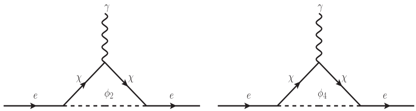
Figure 16: Feynman diagrams contributing to the anomalous magnetic moment.

The expression of $\Delta{a}_{e}$ due to these scalar mediated diagrams is given by Leveille:1977rc

$$\Delta{a}^{scalar}_{e} = -\dfrac{Q^{\chi}_{em}\,m_{e}}{8\pi^{2}}\left[(g^{s}_{\phi_{2}})^{2}\,\mathcal{I}(m_{e},\,M_{\chi},\,M_{\phi_{2}})+(g^{p}_{\phi_{2}})^{2}\,\mathcal{I}(m_{e},\,-M_{\chi},\,M_{\phi_{2}})\right.$$ (65)

$$\left.(g^{s}_{\phi_{4}})^{2}\,\mathcal{I}(m_{e},\,M_{\chi},\,M_{\phi_{4}})+(g^{p}_{\phi_{4}})^{2}\,\mathcal{I}(m_{e},\,-M_{\chi},\,M_{\phi_{4}})\right]\,,$$

where the loop integral function $\mathcal{I}(m_{1},m_{2},m_{3})$ is defined as

$$\mathcal{I}(m_{1},\,m_{2},\,m_{3})=\int_{0}^{1}dx\dfrac{x^{2}-x^{3}+\frac{m_{2}}{m_{1}}x^{2}}{m_{1}^{2}x^{2}+(m_{2}^{2}-m_{1}^{2})x+m^{2}_{3}(1-x)}\,$$ (66)

and the associated coefficients $g^{(s,\,p)}_{({\phi_{2}},\,{\phi_{4}})}$ have the following expressions

$$g^{s}_{\phi_{2}} = -\dfrac{1}{2}\left(\beta^{R}_{e\chi}\cos\theta_{D}-\beta_{e\chi}^{L}\sin\theta_{D}\right),$$

$$g^{p}_{\phi_{2}} = -\dfrac{1}{2}\left(\beta^{R}_{e\chi}\cos\theta_{D}+\beta_{e\chi}^{L}\sin\theta_{D}\right),$$

$$g^{s}_{\phi_{4}} = -\dfrac{1}{2}\left(\beta^{R}_{e\chi}\sin\theta_{D}+\beta_{e\chi}^{L}\cos\theta_{D}\right),$$

$$g^{p}_{\phi_{4}} = -\dfrac{1}{2}\left(\beta^{R}_{e\chi}\sin\theta_{D}-\beta_{e\chi}^{L}\cos\theta_{D}\right).$$ (67)

These are scalar and pseudo scalar couplings of $\phi_{i}$ with $e$ and $\chi$ i.e.  we have an interaction like $\overline{e}\left(g^{s}_{\phi_{i}}+\gamma_{5}\,g^{p}_{\phi_{i}}\right)\chi\phi_{i}$. The total BSM contribution in $(g-2)_{e}$ in the extended model is $\Delta{a}_{e}=\Delta{a}^{scalar}_{e}+\Delta{a}^{Z_{\mu\tau}}_{e}$, where $\Delta{a}^{Z_{\mu\tau}}_{e}$, the contribution due to $Z_{\mu\tau}$, is given in Eq.  (17). However, since there is no new Yukawa coupling for muon, the BSM effect in the anomalous magnetic moment of muon is solely due to $Z_{\mu\tau}$ as also in the minimal $L_{\mu}-L_{\tau}$ model.

Appendix B Necessary Vertex factors

In this appendix we have listed the necessary vertex factors.

$$\phi_{4}\phi_{4}\phi_{4}:-3\sqrt{2}\,\xi v_{\mu\tau}\cos^{3}\theta_{D}\,,$$ (68)

$$\phi^{\dagger}_{4}\phi^{\dagger}_{4}\phi^{\dagger}_{4}:-3\sqrt{2}\,\xi v_{\mu\tau}\cos^{3}\theta_{D}\,,$$ (69)

$$\phi_{4}\phi_{4}\phi^{\dagger}_{4}\phi^{\dagger}_{4}:-4\left(\lambda_{4}\,\cos^{4}\theta_{D}+\lambda_{2}\,\sin^{4}\theta_{D}+\lambda_{24}\sin^{2}\theta_{D}\cos^{2}\theta_{D}\right)\,,$$ (70)

$$h_{1}\phi^{\dagger}_{2}\phi_{4}:-\dfrac{1}{2}\cos\theta\left(\sqrt{2}\,\mu\cos 2\theta_{D}+v(\lambda_{12}+\lambda^{\prime}_{12}-\lambda_{14})\sin 2\theta_{D}\right)$$

$$~{}~{}~{}~{}~{}~{}~{}~{}~{}~{}~{}~{}~{}~{}~{}~{}~{}~{}+v_{\mu\tau}(\lambda_{23}-\lambda_{34})\cos\theta_{D}\sin\theta_{D}\sin\theta\,,$$ (71)

$$h_{1}\phi_{2}\phi^{\dagger}_{4}:-\dfrac{1}{2}\cos\theta\left(\sqrt{2}\,\mu\cos 2\theta_{D}+v(\lambda_{12}+\lambda^{\prime}_{12}-\lambda_{14})\sin 2\theta_{D}\right)$$

$$~{}~{}~{}~{}~{}~{}~{}~{}~{}~{}~{}~{}~{}~{}~{}~{}~{}~{}+v_{\mu\tau}(\lambda_{23}-\lambda_{34})\cos\theta_{D}\sin\theta_{D}\sin\theta\,,$$ (72)

$$h_{3}\phi^{\dagger}_{2}\phi_{2}:-v_{\mu\tau}\cos\theta\left(\lambda_{23}\cos^{2}\theta_{D}+\lambda_{34}\sin^{2}\theta_{D}\right)-\sin\theta\Big{(}-\sqrt{2}\mu\sin\theta_{D}\cos\theta_{D}$$

$$~{}~{}~{}~{}~{}~{}~{}~{}~{}~{}~{}~{}~{}~{}~{}~{}~{}~{}+v\cos^{2}\theta_{D}(\lambda_{12}+\lambda^{\prime}_{12})+\lambda_{14}v\sin^{2}\theta_{D}\Big{)}\,,$$ (73)

$$h_{3}\phi^{\dagger}_{4}\phi_{4}:-v_{\mu\tau}\cos\theta\left(\lambda_{34}\cos^{2}\theta_{D}+\lambda_{23}\sin^{2}\theta_{D}\right)-\sin\theta\Big{(}+\sqrt{2}\mu\sin\theta_{D}\cos\theta_{D}$$

$$~{}~{}~{}~{}~{}~{}~{}~{}~{}~{}~{}~{}~{}~{}~{}~{}~{}~{}+v\sin^{2}\theta_{D}(\lambda_{12}+\lambda^{\prime}_{12})+\lambda_{14}v\cos^{2}\theta_{D}\Big{)}\,,$$ (74)

$$h_{3}\phi_{4}\phi_{4}\phi_{4}:-3\sqrt{2}\,\xi\cos^{3}\theta_{D}\cos\theta\,,$$ (75)

$$h_{3}\phi^{\dagger}_{4}\phi^{\dagger}_{4}\phi^{\dagger}_{4}:-3\sqrt{2}\,\xi\cos^{3}\theta_{D}\cos\theta\,,$$ (76)

$$h_{1}\phi_{4}\phi_{4}\phi_{4}:3\sqrt{2}\,\xi\cos^{3}\theta_{D}\sin\theta\,,$$ (77)

$$h_{1}\phi^{\dagger}_{4}\phi^{\dagger}_{4}\phi^{\dagger}_{4}:3\sqrt{2}\,\xi\cos^{3}\theta_{D}\sin\theta\,,$$ (78)

$$\phi_{2}\phi_{4}\phi_{4}:3\sqrt{2}\,v_{\mu\tau}\,\xi\cos^{2}\theta_{D}\sin\theta_{D}\,,$$ (79)

$$\phi^{\dagger}_{2}\phi^{\dagger}_{4}\phi^{\dagger}_{4}:3\sqrt{2}\,v_{\mu\tau}\,\xi\cos^{2}\theta_{D}\sin\theta_{D}\,,$$ (80)

$$h\phi^{\dagger}_{4}\phi_{4}:-\sin\theta\Big{(}v\lambda_{14}\cos^{2}\theta_{D}+\sqrt{2}\mu\cos\theta_{D}\sin\theta_{D}+v(\lambda_{12}+\lambda_{12}^{\prime})\sin^{2}\theta_{D}\Big{)}+$$

$$v_{\mu\tau}\cos\theta\Big{(}\lambda_{34}\cos^{2}\theta_{D}+\lambda_{23}\sin^{2}\theta_{D}\Big{)}$$ (81)

$$\phi^{\dagger}_{4}(p_{1})\phi_{4}(p_{2})Z:\dfrac{g_{2}}{2\,\cos\theta_{W}}\sin^{2}\theta_{D}(p_{1}-p_{2})^{\alpha}\,,$$ (82)

$$\phi^{\dagger}_{4}(p_{1})\phi_{4}(p_{2})Z_{\mu\tau}:\dfrac{g_{\mu\tau}}{3}(p_{1}-p_{2})^{\alpha}\,.$$ (83)

References

- (1) Y. Sofue and V. Rubin, Rotation curves of spiral galaxies, Ann. Rev. Astron. Astrophys. 39 (2001) 137 [astro-ph/0010594].
- (2) M. Bartelmann and P. Schneider, Weak gravitational lensing, Phys. Rept. 340 (2001) 291 [astro-ph/9912508].
- (3) D. Clowe, A. Gonzalez and M. Markevitch, Weak lensing mass reconstruction of the interacting cluster 1E0657-558: Direct evidence for the existence of dark matter, Astrophys. J. 604 (2004) 596 [astro-ph/0312273].
- (4) Planck collaboration, Planck 2018 results. VI. Cosmological parameters, Astron. Astrophys. 641 (2020) A6 [1807.06209].
- (5) Muon g-2 collaboration, Precise measurement of the positive muon anomalous magnetic moment, Phys. Rev. Lett. 86 (2001) 2227 [hep-ex/0102017].
- (6) Muon g-2 collaboration, Final Report of the Muon E821 Anomalous Magnetic Moment Measurement at BNL, Phys. Rev. D 73 (2006) 072003 [hep-ex/0602035].
- (7) F. Jegerlehner and A. Nyffeler, The Muon g-2, Phys. Rept. 477 (2009) 1 [0902.3360].
- (8) M. Davier, A. Hoecker, B. Malaescu and Z. Zhang, A new evaluation of the hadronic vacuum polarisation contributions to the muon anomalous magnetic moment and to , Eur. Phys. J. C 80 (2020) 241 [1908.00921].
- (9) T. Aoyama et al., The anomalous magnetic moment of the muon in the Standard Model, Phys. Rept. 887 (2020) 1 [2006.04822].
- (10) Muon g-2 collaboration, Measurement of the Positive Muon Anomalous Magnetic Moment to 0.46 ppm, Phys. Rev. Lett. 126 (2021) 141801 [2104.03281].
- (11) Muon g-2 collaboration, Measurement of the anomalous precession frequency of the muon in the Fermilab Muon Experiment, Phys. Rev. D 103 (2021) 072002 [2104.03247].
- (12) M. Abe et al., A New Approach for Measuring the Muon Anomalous Magnetic Moment and Electric Dipole Moment, PTEP 2019 (2019) 053C02 [1901.03047].
- (13) R. H. Parker, C. Yu, W. Zhong, B. Estey and H. Müller, Measurement of the fine-structure constant as a test of the Standard Model, Science 360 (2018) 191 [1812.04130].
- (14) L. Morel, Z. Yao, P. Cladé and S. Guellati-Khélifa, Determination of the fine-structure constant with an accuracy of 81 parts per trillion, Nature 588 (2020) 61.
- (15) J. S. Bell and J. M. Leinaas, Electrons as accelerated thermometers, Nucl. Phys. B 212 (1983) 131.
- (16) A. Anghel, F. Ardana-Lamas, F. Le Pimpec and C. P. Hauri, Large Charge Extraction from Metallic Multifilamentary Nb Sn-3 Photocathode, Phys. Rev. Lett. 108 (2012) 194801.
- (17) X. G. He, G. C. Joshi, H. Lew and R. R. Volkas, NEW Z-prime PHENOMENOLOGY, Phys. Rev. D 43 (1991) 22.
- (18) X.-G. He, G. C. Joshi, H. Lew and R. R. Volkas, Simplest Z-prime model, Phys. Rev. D 44 (1991) 2118.
- (19) E. Ma, D. P. Roy and S. Roy, Gauged L(mu) - L(tau) with large muon anomalous magnetic moment and the bimaximal mixing of neutrinos, Phys. Lett. B 525 (2002) 101 [hep-ph/0110146].
- (20) W. Grimus, S. Kaneko, L. Lavoura, H. Sawanaka and M. Tanimoto, mu-tau antisymmetry and neutrino mass matrices, JHEP 01 (2006) 110 [hep-ph/0510326].
- (21) W. Rodejohann and M. A. Schmidt, Flavor symmetry L(mu) - L(tau) and quasi-degenerate neutrinos, Phys. Atom. Nucl. 69 (2006) 1833 [hep-ph/0507300].
- (22) I. Aizawa and M. Yasue, A New type of complex neutrino mass texture and mu-tau symmetry, Phys. Rev. D 73 (2006) 015002 [hep-ph/0510132].
- (23) Z.-z. Xing, H. Zhang and S. Zhou, Nearly Tri-bimaximal Neutrino Mixing and CP Violation from mu-tau Symmetry Breaking, Phys. Lett. B 641 (2006) 189 [hep-ph/0607091].
- (24) B. Adhikary, Soft breaking of L(mu) - L(tau) symmetry: Light neutrino spectrum and Leptogenesis, Phys. Rev. D 74 (2006) 033002 [hep-ph/0604009].
- (25) K. Fuki and M. Yasue, What does mu-tau symmetry imply in neutrino mixings?, Phys. Rev. D 73 (2006) 055014 [hep-ph/0601118].
- (26) N. Haba and W. Rodejohann, A Supersymmetric contribution to the neutrino mass matrix and breaking of mu-tau symmetry, Phys. Rev. D 74 (2006) 017701 [hep-ph/0603206].
- (27) A. S. Joshipura, B. P. Kodrani and K. M. Patel, Fermion Masses and Mixings in a mu-tau symmetric SO(10), Phys. Rev. D 79 (2009) 115017 [0903.2161].
- (28) B. Adhikary, A. Ghosal and P. Roy, mu tau symmetry, tribimaximal mixing and four zero neutrino Yukawa textures, JHEP 10 (2009) 040 [0908.2686].
- (29) A. S. Joshipura and W. Rodejohann, Scaling in the Neutrino Mass Matrix, mu-tau Symmetry and the See-Saw Mechanism, Phys. Lett. B 678 (2009) 276 [0905.2126].
- (30) Z.-z. Xing and Y.-L. Zhou, A Generic Diagonalization of the 3 x 3 Neutrino Mass Matrix and Its Implications on the Flavor Symmetry and Maximal CP Violation, Phys. Lett. B 693 (2010) 584 [1008.4906].
- (31) T. Araki and C. Q. Geng, \mu-\tau symmetry in Zee-Babu model, Phys. Lett. B 694 (2011) 113 [1006.0629].
- (32) H.-J. He and F.-R. Yin, Common Origin of and CP Breaking in Neutrino Seesaw, Baryon Asymmetry, and Hidden Flavor Symmetry, Phys. Rev. D 84 (2011) 033009 [1104.2654].
- (33) J. Heeck and W. Rodejohann, Gauged Symmetry at the Electroweak Scale, Phys. Rev. D 84 (2011) 075007 [1107.5238].
- (34) W. Grimus and L. Lavoura, mu-tau Interchange symmetry and lepton mixing, Fortsch. Phys. 61 (2013) 535 [1207.1678].
- (35) W. Altmannshofer, S. Gori, M. Pospelov and I. Yavin, Neutrino Trident Production: A Powerful Probe of New Physics with Neutrino Beams, Phys. Rev. Lett. 113 (2014) 091801 [1406.2332].
- (36) Z.-z. Xing and Z.-h. Zhao, A review of - flavor symmetry in neutrino physics, Rept. Prog. Phys. 79 (2016) 076201 [1512.04207].
- (37) K. Asai, K. Hamaguchi and N. Nagata, Predictions for the neutrino parameters in the minimal gauged U(1) model, Eur. Phys. J. C 77 (2017) 763 [1705.00419].
- (38) A. Dev, Gauged - Model with an Inverse Seesaw Mechanism for Neutrino Masses, 1710.02878.
- (39) C.-H. Chen and T. Nomura, Neutrino mass in a gauged model, Nucl. Phys. B 940 (2019) 292 [1705.10620].
- (40) T. Nomura and H. Okada, Zee-Babu type model with gauge symmetry, Phys. Rev. D 97 (2018) 095023 [1803.04795].
- (41) T. Nomura and H. Okada, Neutrino mass generation with large multiplets under local symmetry, Phys. Lett. B 783 (2018) 381 [1805.03942].
- (42) H. Banerjee, P. Byakti and S. Roy, Supersymmetric gauged U(1) model for neutrinos and the muon anomaly, Phys. Rev. D 98 (2018) 075022 [1805.04415].
- (43) W. Altmannshofer, S. Gori, S. Profumo and F. S. Queiroz, Explaining dark matter and B decay anomalies with an model, JHEP 12 (2016) 106 [1609.04026].
- (44) S. Patra, S. Rao, N. Sahoo and N. Sahu, Gauged model in light of muon anomaly, neutrino mass and dark matter phenomenology, Nucl. Phys. B 917 (2017) 317 [1607.04046].
- (45) A. Biswas, S. Choubey and S. Khan, Neutrino Mass, Dark Matter and Anomalous Magnetic Moment of Muon in a Model, JHEP 09 (2016) 147 [1608.04194].
- (46) A. Biswas, S. Choubey and S. Khan, FIMP and Muon () in a U Model, JHEP 02 (2017) 123 [1612.03067].
- (47) A. Biswas, S. Choubey, L. Covi and S. Khan, Explaining the 3.5 keV X-ray Line in a Extension of the Inert Doublet Model, JCAP 02 (2018) 002 [1711.00553].
- (48) G. Arcadi, T. Hugle and F. S. Queiroz, The Dark Rises via Kinetic Mixing, Phys. Lett. B 784 (2018) 151 [1803.05723].
- (49) S. Singirala, S. Sahoo and R. Mohanta, Exploring dark matter, neutrino mass and anomalies in model, Phys. Rev. D 99 (2019) 035042 [1809.03213].
- (50) P. Foldenauer, Light dark matter in a gauged model, Phys. Rev. D 99 (2019) 035007 [1808.03647].
- (51) M. Escudero, D. Hooper, G. Krnjaic and M. Pierre, Cosmology with A Very Light Lμ Lτ Gauge Boson, JHEP 03 (2019) 071 [1901.02010].
- (52) A. Biswas and A. Shaw, Reconciling dark matter, anomalies and in an scenario, JHEP 05 (2019) 165 [1903.08745].
- (53) N. Okada and O. Seto, Inelastic extra charged scalar dark matter, Phys. Rev. D 101 (2020) 023522 [1908.09277].
- (54) D. Borah, S. Mahapatra, D. Nanda and N. Sahu, Inelastic fermion dark matter origin of XENON1T excess with muon and light neutrino mass, Phys. Lett. B 811 (2020) 135933 [2007.10754].
- (55) K. Asai, S. Okawa and K. Tsumura, Search for U(1) charged Dark Matter with neutrino telescope, JHEP 03 (2021) 047 [2011.03165].
- (56) D. Borah, M. Dutta, S. Mahapatra and N. Sahu, Lepton Anomalous Magnetic Moment with Singlet-Doublet Fermion Dark Matter in Scotogenic Model, 2109.02699.
- (57) M. Drees and W. Zhao, for Light Dark Matter, , the keV excess and the Hubble Tension, 2107.14528.
- (58) T. Hapitas, D. Tuckler and Y. Zhang, General Kinetic Mixing in Gauged Model for Muon and Dark Matter, 2108.12440.
- (59) A. Tapadar, S. Ganguly and S. Roy, Non-adiabatic evolution of dark sector in the presence of gauge symmetry, 2109.13609.
- (60) Borexino collaboration, First Simultaneous Precision Spectroscopy of , 7Be, and Solar Neutrinos with Borexino Phase-II, Phys. Rev. D 100 (2019) 082004 [1707.09279].
- (61) W. Altmannshofer, S. Gori, J. Martín-Albo, A. Sousa and M. Wallbank, Neutrino Tridents at DUNE, Phys. Rev. D 100 (2019) 115029 [1902.06765].
- (62) SHiP collaboration, A facility to Search for Hidden Particles (SHiP) at the CERN SPS, 1504.04956.
- (63) M. Bauer, P. Foldenauer and J. Jaeckel, Hunting All the Hidden Photons, JHEP 07 (2018) 094 [1803.05466].
- (64) H. Davoudiasl and W. J. Marciano, Tale of two anomalies, Phys. Rev. D 98 (2018) 075011 [1806.10252].
- (65) A. Crivellin, M. Hoferichter and P. Schmidt-Wellenburg, Combined explanations of and implications for a large muon EDM, Phys. Rev. D 98 (2018) 113002 [1807.11484].
- (66) J. Liu, C. E. M. Wagner and X.-P. Wang, A light complex scalar for the electron and muon anomalous magnetic moments, JHEP 03 (2019) 008 [1810.11028].
- (67) X.-F. Han, T. Li, L. Wang and Y. Zhang, Simple interpretations of lepton anomalies in the lepton-specific inert two-Higgs-doublet model, Phys. Rev. D 99 (2019) 095034 [1812.02449].
- (68) M. Bauer, M. Neubert, S. Renner, M. Schnubel and A. Thamm, Axionlike Particles, Lepton-Flavor Violation, and a New Explanation of and , Phys. Rev. Lett. 124 (2020) 211803 [1908.00008].
- (69) M. Endo and W. Yin, Explaining electron and muon anomaly in SUSY without lepton-flavor mixings, JHEP 08 (2019) 122 [1906.08768].
- (70) M. Badziak and K. Sakurai, Explanation of electron and muon g 2 anomalies in the MSSM, JHEP 10 (2019) 024 [1908.03607].
- (71) G. Hiller, C. Hormigos-Feliu, D. F. Litim and T. Steudtner, Anomalous magnetic moments from asymptotic safety, Phys. Rev. D 102 (2020) 071901 [1910.14062].
- (72) I. Bigaran and R. R. Volkas, Getting chirality right: Single scalar leptoquark solutions to the puzzle, Phys. Rev. D 102 (2020) 075037 [2002.12544].
- (73) M. Endo, S. Iguro and T. Kitahara, Probing flavor-violating ALP at Belle II, JHEP 06 (2020) 040 [2002.05948].
- (74) I. Doršner, S. Fajfer and S. Saad, selecting scalar leptoquark solutions for the puzzles, Phys. Rev. D 102 (2020) 075007 [2006.11624].
- (75) N. Haba, Y. Shimizu and T. Yamada, Muon and electron and the origin of the fermion mass hierarchy, PTEP 2020 (2020) 093B05 [2002.10230].
- (76) L. Calibbi, M. L. López-Ibáñez, A. Melis and O. Vives, Muon and electron and lepton masses in flavor models, JHEP 06 (2020) 087 [2003.06633].
- (77) C.-H. Chen and T. Nomura, Electron and muon , radiative neutrino mass, and in a model, Nucl. Phys. B 964 (2021) 115314 [2003.07638].
- (78) B. Dutta, S. Ghosh and T. Li, Explaining , the KOTO anomaly and the MiniBooNE excess in an extended Higgs model with sterile neutrinos, Phys. Rev. D 102 (2020) 055017 [2006.01319].
- (79) W. Abdallah, R. Gandhi and S. Roy, Understanding the MiniBooNE and the muon and electron anomalies with a light and a second Higgs doublet, JHEP 12 (2020) 188 [2006.01948].
- (80) K.-F. Chen, C.-W. Chiang and K. Yagyu, An explanation for the muon and electron anomalies and dark matter, JHEP 09 (2020) 119 [2006.07929].
- (81) F. J. Botella, F. Cornet-Gomez and M. Nebot, Electron and muon anomalies in general flavour conserving two Higgs doublets models, Phys. Rev. D 102 (2020) 035023 [2006.01934].
- (82) S. Jana, P. K. Vishnu, W. Rodejohann and S. Saad, Dark matter assisted lepton anomalous magnetic moments and neutrino masses, Phys. Rev. D 102 (2020) 075003 [2008.02377].
- (83) C. Hati, J. Kriewald, J. Orloff and A. M. Teixeira, Anomalies in 8Be nuclear transitions and : towards a minimal combined explanation, JHEP 07 (2020) 235 [2005.00028].
- (84) E. J. Chun and T. Mondal, Explaining anomalies in two Higgs doublet model with vector-like leptons, JHEP 11 (2020) 077 [2009.08314].
- (85) S.-P. Li, X.-Q. Li, Y.-Y. Li, Y.-D. Yang and X. Zhang, Power-aligned 2HDM: a correlative perspective on , JHEP 01 (2021) 034 [2010.02799].
- (86) H. Banerjee, B. Dutta and S. Roy, Supersymmetric gauged model for electron and muon anomaly, JHEP 03 (2021) 211 [2011.05083].
- (87) J. Cao, Y. He, J. Lian, D. Zhang and P. Zhu, Electron and muon anomalous magnetic moments in the inverse seesaw extended NMSSM, Phys. Rev. D 104 (2021) 055009 [2102.11355].
- (88) L. Delle Rose, S. Khalil and S. Moretti, Explaining electron and muon 2 anomalies in an Aligned 2-Higgs Doublet Model with right-handed neutrinos, Phys. Lett. B 816 (2021) 136216 [2012.06911].
- (89) P. Escribano, J. Terol-Calvo and A. Vicente, in an extended inverse type-III seesaw model, Phys. Rev. D 103 (2021) 115018 [2104.03705].
- (90) M. Frank, Y. Hiçyılmaz, S. Mondal, O. Özdal and C. S. Ün, Electron and muon magnetic moments and implications for dark matter and model characterisation in non-universal U(1)’ supersymmetric models, JHEP 10 (2021) 063 [2107.04116].
- (91) H. Bharadwaj, S. Dutta and A. Goyal, Leptonic g 2 anomaly in an extended Higgs sector with vector-like leptons, JHEP 11 (2021) 056 [2109.02586].
- (92) Y. Hochberg, E. Kuflik, T. Volansky and J. G. Wacker, Mechanism for Thermal Relic Dark Matter of Strongly Interacting Massive Particles, Phys. Rev. Lett. 113 (2014) 171301 [1402.5143].
- (93) Y. Hochberg, E. Kuflik, H. Murayama, T. Volansky and J. G. Wacker, Model for Thermal Relic Dark Matter of Strongly Interacting Massive Particles, Phys. Rev. Lett. 115 (2015) 021301 [1411.3727].
- (94) Y. Hochberg, E. Kuflik and H. Murayama, SIMP Spectroscopy, JHEP 05 (2016) 090 [1512.07917].
- (95) N. Daci, I. De Bruyn, S. Lowette, M. H. G. Tytgat and B. Zaldivar, Simplified SIMPs and the LHC, JHEP 11 (2015) 108 [1503.05505].
- (96) N. Bernal and X. Chu, SIMP Dark Matter, JCAP 01 (2016) 006 [1510.08527].
- (97) N. Bernal, C. Garcia-Cely and R. Rosenfeld, WIMP and SIMP Dark Matter from the Spontaneous Breaking of a Global Group, JCAP 04 (2015) 012 [1501.01973].
- (98) H. M. Lee and M.-S. Seo, Communication with SIMP dark mesons via Z’ -portal, Phys. Lett. B 748 (2015) 316 [1504.00745].
- (99) S.-M. Choi and H. M. Lee, SIMP dark matter with gauged Z3 symmetry, JHEP 09 (2015) 063 [1505.00960].
- (100) S.-M. Choi, Y.-J. Kang and H. M. Lee, On thermal production of self-interacting dark matter, JHEP 12 (2016) 099 [1610.04748].
- (101) S.-M. Choi, Y. Hochberg, E. Kuflik, H. M. Lee, Y. Mambrini, H. Murayama et al., Vector SIMP dark matter, JHEP 10 (2017) 162 [1707.01434].
- (102) S.-M. Choi, H. M. Lee and M.-S. Seo, Cosmic abundances of SIMP dark matter, JHEP 04 (2017) 154 [1702.07860].
- (103) S.-Y. Ho, T. Toma and K. Tsumura, A Radiative Neutrino Mass Model with SIMP Dark Matter, JHEP 07 (2017) 101 [1705.00592].
- (104) J. H. Davis, Probing Sub-GeV Mass Strongly Interacting Dark Matter with a Low-Threshold Surface Experiment, Phys. Rev. Lett. 119 (2017) 211302 [1708.01484].
- (105) Y. Hochberg, E. Kuflik, R. Mcgehee, H. Murayama and K. Schutz, Strongly interacting massive particles through the axion portal, Phys. Rev. D 98 (2018) 115031 [1806.10139].
- (106) S. Bhattacharya, P. Ghosh and S. Verma, SIMPler realisation of Scalar Dark Matter, JCAP 01 (2020) 040 [1904.07562].
- (107) J. Smirnov and J. F. Beacom, New Freezeout Mechanism for Strongly Interacting Dark Matter, Phys. Rev. Lett. 125 (2020) 131301 [2002.04038].
- (108) A. Katz, E. Salvioni and B. Shakya, Split SIMPs with Decays, JHEP 10 (2020) 049 [2006.15148].
- (109) S.-M. Choi, J. Kim, P. Ko and J. Li, A multi-component SIMP model with , JHEP 09 (2021) 028 [2103.05956].
- (110) A. Bilal, Lectures on Anomalies, 0802.0634.
- (111) S. L. Adler, Axial vector vertex in spinor electrodynamics, Phys. Rev. 177 (1969) 2426.
- (112) W. A. Bardeen, Anomalous Ward identities in spinor field theories, Phys. Rev. 184 (1969) 1848.
- (113) R. Delbourgo and A. Salam, The gravitational correction to pcac, Phys. Lett. B 40 (1972) 381.
- (114) T. Eguchi and P. G. O. Freund, Quantum Gravity and World Topology, Phys. Rev. Lett. 37 (1976) 1251.
- (115) D. Hanneke, S. Fogwell and G. Gabrielse, New Measurement of the Electron Magnetic Moment and the Fine Structure Constant, Phys. Rev. Lett. 100 (2008) 120801 [0801.1134].
- (116) CMS collaboration, Search for an gauge boson using Z events in proton-proton collisions at 13 TeV, Phys. Lett. B 792 (2019) 345 [1808.03684].
- (117) BaBar collaboration, Search for a muonic dark force at BABAR, Phys. Rev. D 94 (2016) 011102 [1606.03501].
- (118) Muon Collider collaboration, The physics case of a 3 TeV muon collider stage, in 2022 Snowmass Summer Study, 3, 2022, 2203.07261.
- (119) G. Krnjaic, G. Marques-Tavares, D. Redigolo and K. Tobioka, Probing Muonphilic Force Carriers and Dark Matter at Kaon Factories, Phys. Rev. Lett. 124 (2020) 041802 [1902.07715].
- (120) S. N. Gninenko, N. V. Krasnikov and V. A. Matveev, Muon g-2 and searches for a new leptophobic sub-GeV dark boson in a missing-energy experiment at CERN, Phys. Rev. D 91 (2015) 095015 [1412.1400].
- (121) Y. Kahn, G. Krnjaic, N. Tran and A. Whitbeck, M3: a new muon missing momentum experiment to probe (g2)μ and dark matter at Fermilab, JHEP 09 (2018) 153 [1804.03144].
- (122) ATLAS collaboration, Observation of a new particle in the search for the Standard Model Higgs boson with the ATLAS detector at the LHC, Phys. Lett. B 716 (2012) 1 [1207.7214].
- (123) CMS collaboration, Observation of a New Boson at a Mass of 125 GeV with the CMS Experiment at the LHC, Phys. Lett. B 716 (2012) 30 [1207.7235].
- (124) P. Minkowski, at a Rate of One Out of Muon Decays?, Phys. Lett. B 67 (1977) 421.
- (125) T. Yanagida, Horizontal gauge symmetry and masses of neutrinos, Conf. Proc. C 7902131 (1979) 95.
- (126) R. N. Mohapatra and G. Senjanovic, Neutrino Mass and Spontaneous Parity Nonconservation, Phys. Rev. Lett. 44 (1980) 912.
- (127) J. Schechter and J. W. F. Valle, Neutrino Masses in SU(2) x U(1) Theories, Phys. Rev. D 22 (1980) 2227.
- (128) Planck collaboration, Planck 2015 results. XIII. Cosmological parameters, Astron. Astrophys. 594 (2016) A13 [1502.01589].
- (129) P. F. de Salas, D. V. Forero, C. A. Ternes, M. Tortola and J. W. F. Valle, Status of neutrino oscillations 2018: 3 hint for normal mass ordering and improved CP sensitivity, Phys. Lett. B 782 (2018) 633 [1708.01186].
- (130) E. D. Carlson, M. E. Machacek and L. J. Hall, Self-interacting dark matter, Astrophys. J. 398 (1992) 43.
- (131) A. Biswas, S. Ganguly and S. Roy, When Freeze-out occurs due to a non-Boltzmann suppression: A study of degenerate dark sector, JHEP 06 (2021) 108 [2011.02499].
- (132) A. Berlin, D. Hooper and G. Krnjaic, Thermal Dark Matter From A Highly Decoupled Sector, Phys. Rev. D 94 (2016) 095019 [1609.02555].
- (133) A. Belyaev, N. D. Christensen and A. Pukhov, CalcHEP 3.4 for collider physics within and beyond the Standard Model, Comput. Phys. Commun. 184 (2013) 1729 [1207.6082].
- (134) A. Alloul, N. D. Christensen, C. Degrande, C. Duhr and B. Fuks, FeynRules 2.0 - A complete toolbox for tree-level phenomenology, Comput. Phys. Commun. 185 (2014) 2250 [1310.1921].
- (135) M. Markevitch, A. H. Gonzalez, D. Clowe, A. Vikhlinin, L. David, W. Forman et al., Direct constraints on the dark matter self-interaction cross-section from the merging galaxy cluster 1E0657-56, Astrophys. J. 606 (2004) 819 [astro-ph/0309303].
- (136) S. Tulin and H.-B. Yu, Dark Matter Self-interactions and Small Scale Structure, Phys. Rept. 730 (2018) 1 [1705.02358].
- (137) H.-Y. Cheng and C.-W. Chiang, Revisiting Scalar and Pseudoscalar Couplings with Nucleons, JHEP 07 (2012) 009 [1202.1292].
- (138) XENON collaboration, Constraining the spin-dependent WIMP-nucleon cross sections with XENON1T, Phys. Rev. Lett. 122 (2019) 141301 [1902.03234].
- (139) R. Essig, J. Mardon and T. Volansky, Direct Detection of Sub-GeV Dark Matter, Phys. Rev. D 85 (2012) 076007 [1108.5383].
- (140) R. Essig, M. Fernandez-Serra, J. Mardon, A. Soto, T. Volansky and T.-T. Yu, Direct Detection of sub-GeV Dark Matter with Semiconductor Targets, JHEP 05 (2016) 046 [1509.01598].
- (141) V. A. Rubakov and D. S. Gorbunov, Introduction to the Theory of the Early Universe: Hot big bang theory. World Scientific, Singapore, 2017, 10.1142/10447.
- (142) P. Gondolo, J. Hisano and K. Kadota, The Effect of quark interactions on dark matter kinetic decoupling and the mass of the smallest dark halos, Phys. Rev. D 86 (2012) 083523 [1205.1914].
- (143) A. Biswas, D. Borah and D. Nanda, Light Dirac neutrino portal dark matter with observable Neff, JCAP 10 (2021) 002 [2103.05648].
- (144) CMS collaboration, Search for invisible decays of a Higgs boson produced through vector boson fusion in proton-proton collisions at 13 TeV, Phys. Lett. B 793 (2019) 520 [1809.05937].
- (145) D. Durnford and M.-C. Piro, The search for Light Dark Matter with NEWS-G, 2111.02796.
- (146) SuperCDMS collaboration, Low-mass dark matter search with CDMSlite, Phys. Rev. D 97 (2018) 022002 [1707.01632].
- (147) DarkSide collaboration, Low-Mass Dark Matter Search with the DarkSide-50 Experiment, Phys. Rev. Lett. 121 (2018) 081307 [1802.06994].
- (148) XENON collaboration, Dark Matter Search Results from a One Ton-Year Exposure of XENON1T, Phys. Rev. Lett. 121 (2018) 111302 [1805.12562].
- (149) DARWIN collaboration, DARWIN: towards the ultimate dark matter detector, JCAP 11 (2016) 017 [1606.07001].
- (150) CLIC Physics Working Group collaboration, Physics at the CLIC multi-TeV linear collider, in 11th International Conference on Hadron Spectroscopy, CERN Yellow Reports: Monographs, 6, 2004, DOI [hep-ph/0412251].
- (151) D. Dannheim, P. Lebrun, L. Linssen, D. Schulte, F. Simon, S. Stapnes et al., CLIC e+e- Linear Collider Studies, 1208.1402.
- (152) Physics and Detectors at CLIC: CLIC Conceptual Design Report, 1202.5940.
- (153) CLIC Detector, Physics Study collaboration, Physics at the CLIC e+e- Linear Collider – Input to the Snowmass process 2013, in Community Summer Study 2013: Snowmass on the Mississippi, 7, 2013, 1307.5288.
- (154) CLICdp collaboration, CLICdet: The post-CDR CLIC detector model, .
- (155) CLIC accelerator collaboration, The Compact Linear Collider (CLIC) - Project Implementation Plan, 1903.08655.
- (156) The International Linear Collider Technical Design Report - Volume 1: Executive Summary, 1306.6327.
- (157) The International Linear Collider Technical Design Report - Volume 3.II: Accelerator Baseline Design, 1306.6328.
- (158) H. Abramowicz et al., The International Linear Collider Technical Design Report - Volume 4: Detectors, 1306.6329.
- (159) The International Linear Collider Technical Design Report - Volume 2: Physics, 1306.6352.
- (160) The International Linear Collider Technical Design Report - Volume 3.I: Accelerator \& in the Technical Design Phase, 1306.6353.
- (161) J. Alwall, R. Frederix, S. Frixione, V. Hirschi, F. Maltoni, O. Mattelaer et al., The automated computation of tree-level and next-to-leading order differential cross sections, and their matching to parton shower simulations, JHEP 07 (2014) 079 [1405.0301].
- (162) J. Alwall, M. Herquet, F. Maltoni, O. Mattelaer and T. Stelzer, MadGraph 5 : Going Beyond, JHEP 06 (2011) 128 [1106.0522].
- (163) CMS collaboration, Searches for pair production of charginos and top squarks in final states with two oppositely charged leptons in proton-proton collisions at 13 TeV, JHEP 11 (2018) 079 [1807.07799].
- (164) T. Sjostrand, S. Mrenna and P. Z. Skands, PYTHIA 6.4 Physics and Manual, JHEP 05 (2006) 026 [hep-ph/0603175].
- (165) DELPHES 3 collaboration, DELPHES 3, A modular framework for fast simulation of a generic collider experiment, JHEP 02 (2014) 057 [1307.6346].
- (166) M. Selvaggi, DELPHES 3: A modular framework for fast-simulation of generic collider experiments, J. Phys. Conf. Ser. 523 (2014) 012033.
- (167) A. Mertens, New features in Delphes 3, J. Phys. Conf. Ser. 608 (2015) 012045.
- (168) J. P. Leveille, The Second Order Weak Correction to (G-2) of the Muon in Arbitrary Gauge Models, Nucl. Phys. B 137 (1978) 63.