Abstract

We introduce a generalized notion of finiteness that provides a structural principle for the set of effective theories that can be consistently coupled to quantum gravity. More concretely, we propose a Tameness Conjecture that states that all valid effective theories are labelled by a definable parameter space and must have scalar field spaces and coupling functions that are definable using the tame geometry built from an o-minimal structure. We give a brief introduction to tame geometry and describe how it restricts sets, manifolds, and functions. We then collect evidence for the Tameness Conjecture by studying various effective theories arising from string theory compactifications by using some recent advances in tame geometry. In particular, we will exploit the fact that coset spaces and period mappings are definable in an o-minimal structure and argue for non-trivial tameness results in higher-supersymmetric theories and in Calabi-Yau compactifications. As strongest evidence for the Tameness Conjecture over a discrete parameter space, we then discuss a recent theorem stating that the locus of self-dual flux vacua of F-theory admits a tame geometry even if one allows for any flux choice satisfying the tadpole constraint. This result implies the finiteness of self-dual flux vacua in F-theory.

1 Introduction and a conjecture

In recent years the search for general principles restricting the form of any effective theories that can be consistently coupled to quantum gravity has attracted much attention [1, 2]. These principles have been formulated in a number of quantum gravity or ‘swampland’ conjectures. They aim to discriminate consistent effective theories that are part of the landscape, from those that are fundamentally flawed and reside in the swampland. One of such principles is the claim that the number of effective theories that are valid below a fixed cut-off scale that are consistent with quantum gravity is finite [3, 4, 5]. The finiteness of effective theories implies constraints on the allowed scalar potentials and the scalar field spaces on which the effective theory is valid, since a new effective theory can arise when lowering the energy scale and settling in a new vacuum. Despite the fact that this clearly restricts valid effective theories, it has not been clear how to turn this into a structural principle. The aim of this work is to introduce a mathematical structure –a tame geometry– and argue that it provides a concrete way to implement finiteness constraints on the set of consistent effective theories. Furthermore, we conjecture that it should be used as a novel general principle to constrain field spaces and coupling functions of UV-completable effective theories.

In this paper we will give a novel perspective on the set of consistent effective theories by claiming that the landscape admits a certain well-defined geometric structure. More precisely, we will propose a Tameness Conjecture that constrains the set of all effective theories that are valid up to some fixed finite energy cut-off scale and can be consistently coupled to quantum gravity. We conjecture that all such theories are labelled by a parameter space that is definable in a so-called o-minimal structure. Furthermore, we claim that also the scalar field spaces and coupling functions, which might depend on these parameters, are definable in the same o-minimal structure. O-minimal structures implement finiteness on a fundamental level and are the prime example of a topologie modérée, a tame topology, envisioned by Grothendieck [6]. Grothendieck’s vision was to develop a topology for geometers that excludes pathological situations that can arise in classical topology. Notably, o-minimal structures can be defined over the real numbers and provide an extension of real algebraic geometry while keeping some of its powerful results intact. They thus provide us with a framework to leave the world of complex geometry, which is often only occurring in effective theories due to the presence of supersymmetry, while setting a completely new focus on finiteness and tameness. It is interesting to highlight that the original interest on o-minimal structures arose from model theory, which is a part of mathematical logic that studies the relationship between formal theories and their models. By now, however, these structures have found applications in several fields of mathematics reaching from number theory to geometry.

The basic strategy in defining a tame topology based on o-minimal structures [7] is to specify the space of allowed subsets of $\mathbb{R}^{n}$, for every $n$. On this space of ‘tame sets’, also called definable sets, one can then define ‘tame functions’, which are termed definable functions. Hereby one always means that these sets and functions are defined with respect to a specified o-minimal structure. The fundamental tameness property of each o-minimal structure is the fact that the only definable sets in one real dimension are the finite union of points and intervals. This property becomes powerful when combined with the requirement that all linear projections of higher-dimensional sets eventually reduce to sets of this type on the real line. Tame topology hereby treats a connected set of infinitely many points, such as an interval or the full real line, as a single object. While the simplest example of an o-minimal structure is formed by collecting sets that are defined by polynomial equalities and inequalities, the existence of much richer o-minimal structures will be central in this work. Firstly, it is a remarkable mathematical fact that extensions exist in which the sets can be defined by also using transcendental functions. In particular, an important result of Wilkie [8], which states that adding the real exponential function does not violate the tameness axioms, has allowed mathematicians to use o-minimal structures in a wide set of geometric applications, such as the Hodge theory application that we will exploit in this work. Secondly, it is apparent that such extensions are needed to describe well-known physical settings since many effective theories cannot be described by purely algebraic data. In particular, instanton corrections to coupling functions should be consistent with the Tameness Conjecture and hence describable within tame geometry. It is interesting that o-minimal structures are, on the one hand, rich enough for many applications, while on the other hand they possess strong finiteness constraints.

To provide evidence for the Tameness Conjecture, we will have a detailed look at some of the well-understood effective actions derived from string theory. String theory has only one free parameter, the string length, and the ten-dimensional effective supergravity actions admit simple scalar field spaces for the arising massless scalars. At the two-derivative level the Tameness Conjecture is readily shown in these highly supersymmetric settings. However, if we consider the theories on a compact manifold, it is well-known that a plethora of effective theories will arise in less than ten dimensions. The scalar field spaces of these effective theories can be very involved and numerous new parameters arise from the geometry of the compactification space and possible backgrounds for the other fields of the higher-dimensional theory, such as background fluxes. It turns out that in theories with more than 8 supercharges, supersymmetry together with some simple-to-state finiteness conditions already ensures that the Tameness Conjecture holds. We will argue that this conclusion requires us to use some recent mathematical results about the tameness of double cosets, i.e. arithmetic quotients of the form $\mathcal{M}_{\Gamma,G,K}=\Gamma\backslash G/K$. The Tameness Conjecture is then satisfied if the free parameter choices, e.g. labelling the allowed groups $G$ and $\Gamma$, are finite. Showing finiteness statements of this type is the aim of much current research [10, 11, 12, 13, 14, 15, 16, 17, 18, 19, 20, 21, 22].

When reducing the amount of supersymmetry, the Tameness Conjecture provides a more independent criterium from this symmetry, since one can find field spaces and coupling functions that are compatible with supergravity but are not tame. Nevertheless, we will show that in some of the best understood string compactifications we only encounter field spaces and coupling functions that are definable in an o-minimal structure. More precisely, we will look at compactifications of Type II string theory on Calabi-Yau threefolds leading to four-dimensional effective theories with $\mathcal{N}=2$ supersymmetry. In these cases the field spaces are built from the moduli spaces of the compact geometry and we will argue that these admit a tame geometry. Moreover, we will introduce a recent foundational result of Bakker, Klingler, Tsimerman [23] that shows that the period mapping is definable in an o-minimal structure denoted by $\mathbb{R}_{\rm an,exp}$. We use this result to argue that at least in the vector sector of $\mathcal{N}=2$ actions arising from Calabi-Yau compactifications the scalar field space metric and gauge coupling function are definable. This provides a very non-trivial test of the Tameness Conjecture if one makes a choice for the topology of the Calabi-Yau manifold. Picking different topologies should be viewed as picking different discrete parameters of the effective theory and the Tameness Conjecture asserts that there are only finitely many such choices.

It is a central statement of the Tameness Conjecture that all viable scalar potentials are definable in an o-minimal structure. This statement ensures finiteness when lowering the cut-off scale of the theory further. Indeed, if after lowering the cut-off some of the fields are too heavy and need to be integrated out, tameness of the original scalar potential will ensure that the resulting new low-energy scalar field space is also definable in an o-minimal structure. In the last part of this work we will provide evidence for this property of the scalar potential in flux compactifications of Type IIB string theory and F-theory reviewed in [24, 25, 26]. These compactifications yield a well-understood class of effective theories with $\mathcal{N}=1$ supersymmetry that admit a positive definite scalar potential solely induced by background fluxes. The Minkowski vacua of this potential arise if the fields adjust such that the fluxes become (imaginary) self-dual. These vacua admit well-defined lifts to higher dimensions and we expect the effective theory with $\mathcal{N}=1$ or $\mathcal{N}=0$ obtained when integrating out the massive scalar field to be well-behaved. We will argue that the flux scalar potential is definable in the o-minimal structure $\mathbb{R}_{\rm an,exp}$ following [23] for fixed fluxes. In this setting, however, we can go further and treat the fluxes as discrete parameters. Definability is retained if the fluxes satisfy the tadpole cancellation condition and we consider the potential sufficiently close to a Minkowski vacuum. This will follow from a result of Bakker, Schnell, Tsimerman, and the author [27], which states that the locus of self-dual fluxes is definable in the o-minimal structure $\mathbb{R}_{\rm an,exp}$. We will briefly summarize the argument and explain how it shows the finiteness of flux choices. Evidence for such a finiteness result has appeared previously in [28, 29, 30, 31, 32, 33, 34]. The theorem of [27] generalizes a famous theorem of Cattani, Deligne, Kaplan [35] proving the finiteness of Hodge classes satisfying a ‘tadpole cancellation condition’.

Let us close by stating the Tameness Conjecture in a weak and a strong form, where the latter specifies an o-minimal structure that suffices in all considered string theory examples: Tameness Conjecture
All effective theories valid below a fixed finite energy cut-off scale that can be consistently coupled to quantum gravity are labelled by a definable parameter space and must have scalar field spaces and coupling functions that are definable in an o-minimal structure. Strong Tameness Conjecture
The o-minimal structure that makes the effective theory definable is $\mathbb{R}_{\rm an,exp}$.

This paper is organized as follows. In section 2 we explain in more detail which aspects of an effective theory we are considering in this work. In particular, we introduce the relevant notion of parameter space, scalar field space, the coupling functions of an effective theory. We then comment on various effective theories arising in string compactifications and highlight additional challenges that need to be faced when a scalar potential is present. In section 3 we then give a lightning introduction to o-minimal structures and tame topology with a focus on some of the foundational results. This will help to clarify the statement of the Tameness Conjecture and provide the background for the more advanced results used in the third part of this work. In fact, in section 4 we will introduce the evidence for the Tameness Conjecture, by discussing various string theory compactifications. In particular, we will also sketch the argument that the flux scalar potential is a tame function and that there are only finitely many self-dual fluxes.

2 On effective theories and their coupling functions

The Tameness Conjecture claims that the scalar field spaces and coupling functions in any effective theory that can be consistently coupled to quantum gravity are definable in a tame geometry introduced in section 3. To make this more concrete let us consider a set of scalar fields $\phi^{i}$ and gauge fields $A^{C}$ coupled to Einstein gravity. In addition to these fields, the effective theory can also contain other fields, such as fermions or higher-form fields, but we will not display them in the following. Then the Lagrangian of the effective theory then schematically takes the form

$$\mathcal{L}=R-g_{ij}(\phi,\lambda)\ D_{\mu}\phi^{i}D^{\mu}\phi^{j}-f_{AB}(\phi,\lambda)\ F^{A}_{\mu\nu}F^{B\,\mu\nu}-V(\phi,\lambda)+\ldots\ ,$$ (2.1)

where $V$ is the scalar potential of the theory. Let us denote by $\mathcal{M}_{\lambda}$ the field space spanned by the $\phi^{i}$ with metric $g_{ij}$. In general, the coupling functions $g_{ij},f_{AB},V,\ldots$ will vary over $\mathcal{M}_{\lambda}$. In addition, we will allow for the field space $\mathcal{M}_{\lambda}$ and the coupling functions to depend on a set of parameters $\lambda_{\alpha}$, which we consider to be part of a parameter space $\mathcal{P}$. These parameters can be vacuum expectation values of fields that have been integrated out, or they can be discrete parameters. Hence, the space $\mathcal{P}$ does not have to be a smooth manifold, but rather can be just some general set. The Tameness Conjecture both restricts the geometry of the set

$$\mathcal{D}=\{(\phi^{i},\lambda_{\alpha}),\ \phi\in\mathcal{M}_{\lambda},\,\lambda\in\mathcal{P}\}$$ (2.2)

as well as the behavior of the coupling functions, such as $g_{ij},f_{AB},V$. The crucial point is here, that we view these coupling functions as maps valued on $\mathcal{D}$ with a set of special tameness properties introduced in section 3.

In this section we recall some effective theories arising in compactifications of string theory. This will allow us to highlight some necessary requirements on the geometry of the Tameness Conjecture that need to be satisfied in order that it is general enough to apply to well-understood examples. Clearly, our discussion will not be exhaustive and should only be seen as a motivation for the structures introduced later. In a first step, we will concentrate on theories without scalar potential in subsection 2.1. We discuss the inclusion of a scalar potential in subsection 2.2 and point out some additional complications arising in this case. The reader familiar with string compactifications does not need to spend much time on this section.

2.1 On scalar field spaces and coupling functions in string compactifications

String theory is originally formulated in ten space-time dimensions. We note that already in ten dimensions all five string theories have massless scalar fields. In particular, Type IIB string theory has a complex scalar $\tau$, the dilaton-axion that takes values on a field space $\text{SL}(2,\mathbb{Z})\backslash SL(2,\mathbb{R})/SO(2)$. This space is non-compact, but admits a complex algebraic structure. While this space has much structure, it turns out that this is not a general feature of the field spaces arising in string theory, but rather a remnant of supersymmetry. In particular, the complex algebraic structure is not necessarily present when looking at string compactifications. To see this, recall that the moduli space of a torus $T^{d}$ is the arithmetic quotient, sometimes called double coset, $SO(d,d;\mathbb{Z})\backslash SO(d,d;\mathbb{R})/SO(d)\times SO(d)$. Purely for dimensional reasons this space is not always complex. The fact that such arithmetic quotients arise as field spaces can be tied to the presence of some supersymmetry in the effective theory. In fact, for more than 8 supercharges, the field spaces take the general form

$$\mathcal{M}_{\Gamma,G,K}=\Gamma\backslash G/K\ ,$$ (2.3)

where $\Gamma$ is a lattice and $K$ is a maximal compact subgroup of $G$. In these supersymmetric theories also the coupling functions take a particularly simple form. Roughly speaking these functions can always expressed as (quotients of) polynomials in a suitable set of coordinates on the field space $\mathcal{M}$. This simple form is compatible with the fact that instanton corrections are often forbidden by supersymmetry.

More involved examples of field spaces and coupling functions arise when compactifying string theory on a Calabi-Yau threefold such that the resulting four-dimensional theory has 8 supercharges or less. If one insists that the Calabi-Yau condition is preserved then the deformation spaces of these spaces split into complex structure and Kähler structure deformations. In the following we will review some facts about the complex structure moduli space $\mathcal{M}_{\rm cs}$, keeping in mind that the geometry of the Kähler structure moduli space is a special case of this more general discussion after using mirror symmetry. For polarized Calabi-Yau threefolds $Y_{3}$ the moduli space $\mathcal{M}_{\rm cs}$ is quasi-projective [36] and non-compact. It has complex dimension $h^{2,1}=\text{dim}H^{2,1}(Y_{3})$ and we will use local coordinates $z^{i}$, $i=1,...,h^{2,1}$ in the following. The natural metric on $\mathcal{M}_{\rm cs}$ that arises in string theory effective actions is the so-called Weil-Petersson metric $g_{i\bar{\jmath}}$. This metric is Kähler and can be derived from a Kähler potential $K=-\log i\bar{\Pi}^{I}\eta_{IJ}\Pi^{J}$. Here $\eta_{IJ}=\gamma_{I}\cap\gamma_{J}$ is the intersection matrix of a basis of three-cycles $\gamma_{I}$ and we have abbreviated

$$\Pi^{I}(z)=\int_{\gamma_{I}}\Omega\ .$$ (2.4)

These integrals are known as period integrals, or periods for short, of the, up to rescaling, unique $(3,0)$-form $\Omega$. The resulting metric takes the form

$$g_{i\bar{\jmath}}=\partial_{z^{i}}\partial_{\bar{z}^{j}}K=\frac{\eta_{IJ}(D_{i}\Pi^{I})(\overline{D_{j}\Pi}\phantom{\Pi}^{\!\!\!\!\!\!J})}{\eta_{KL}\Pi^{K}\bar{\Pi}^{L}}\ ,$$ (2.5)

where $D_{i}\Pi^{I}=(\partial_{z^{i}}+\partial_{z^{i}}K)\Pi^{I}$.

The periods also determine some of the other couplings of the effective theory. For example, consider Type IIB string theory on $Y_{3}$. In the four-dimensional effective theory arising after compactification also the gauge coupling functions $f_{AB}$ for the R-R U(1)s can be expressed in terms of the periods $\Pi$. To explicitly give $f_{AB}$, we first need to introduce a symplectic homology basis $\gamma_{I}=(\gamma^{A},\tilde{\gamma}_{B}$, such that $\gamma^{A}\cap\gamma^{B}=\tilde{\gamma}_{A}\cap\tilde{\gamma}_{B}=0$ and $\gamma^{A}\cap\tilde{\gamma}_{B}=\delta^{A}_{B}$. This allows us to split $\Pi=(\Pi^{A},\Pi_{B})$ and the $\mathcal{N}=2$ gauge coupling function is then given by

$$f_{AB}=(\Pi_{A},\overline{D_{j}\Pi}\phantom{\Pi}_{\!\!\!\!\!A})(\Pi^{B},\overline{D_{j}\Pi}\phantom{\Pi}^{\!\!\!\!\!B})^{-1}\ .$$ (2.6)

Hence, in order that the Tameness Conjecture for coupling functions can possibly be true, it has to hold at least for the couplings (2.5) and (2.6) derived from the period map.

The periods $\Pi^{I}$ are holomorphic but, in general, complicated transcendental functions. However, it is known from the work of Schmid [37] that in a sufficiently small neighbourhood near every boundary of $\mathcal{M}_{\rm cs}$ they admit an expansion that splits them into a polynomial plus exponentially suppressed part. Let us pick coordinates $t^{\alpha},\zeta^{a}$, such that the considered boundary is at $t^{\alpha}=i\infty$ and $\zeta^{a}$ finite. Then one can expand

$$\Pi=e^{t^{i}N_{i}}\Big{(}a_{0}+\sum_{r_{i}}e^{2\pi r_{i}t^{i}}a_{r_{1},...,r_{n}}\Big{)}\ ,$$ (2.7)

where the $N_{i}$ are nilpotent matrices and the coefficients $a_{\bullet}$ can still vary holomorphically with $\zeta^{a}$. Focusing on the behaviour in the $t^{i}$, this implies that the metric $g_{ij}$ will in general involve finitely many polynomial terms as well as a host of exponentially suppressed corrections. This rather constrained behaviour in the asymptotic, non-compact directions, will reappear in a much more general way in the tame geometry introduced in section 3. In fact, it will turn out to be one of the hallmarks of tameness that only a certain set of functions can arise on such non-compact tails. Before explaining this in detail, let us discuss some further issues that arise when one includes a scalar potential.

2.2 Scalar potentials and the challenges to implement finiteness

An additional challenge in understanding the structure of the landscape of the effective theories arises when one includes a potential for the fields, since then a cut-off dependence is apparent. To make this clearer, let us consider an effective theory with a cut-off $\Lambda$. For simplicity, we will only discuss bosonic scalars $\phi^{i}$ in the following and focus on the scalar potential $V(\phi,\lambda)$. The scalar potentials varies over $\mathcal{D}$ defined in (2.2), where $\mathcal{M}_{\lambda}$ is the field space and $\mathcal{P}$ is a space of parameters. The notion of effective potential and $\mathcal{M}_{\lambda}$ will change when lowering the cut-off, say to $\hat{\Lambda}<\Lambda$. In this case some of the $\phi^{i}$ might have masses above this scale and have to be integrated out. Classically, this can be done by solving the vacuum conditions $\partial_{\phi^{k}}V=0$ for the massive fields. Clearly, there might be several solutions to this equation and, depending on our choice of solutions, we end up with a different effective theory. The field space $\mathcal{M}(\Lambda)$ can thus reduce to $\mathcal{M}(\hat{\Lambda})=\cup_{\alpha}\mathcal{M}_{\alpha}$, where $\mathcal{M}_{\alpha}$ is the field space associated to the $\alpha$th effective theory. To each of these theories a parameter space $\mathcal{P}_{\alpha}$ can appear, which now might include the vacuum expectation values of the fields that have been integrated out. Note that if we continue lowering the cut-off, eventually only the massless fields with a moduli space will remain and the effective theories will not have any potential.

The Tameness Conjecture claims that there is a constraint on allowed scalar potentials. It was motivated by the aim to implement finiteness of effective theories below a certain cut-off. Hence, we can again highlight some of the necessary properties of the tame geometry such that this is actually achieved. In fact, finiteness is to demand that for every viable $\mathcal{M}$ and $V(\phi)$ only finitely many $\mathcal{M}_{\alpha}$ can arise when lowering the cut-off. In particular, this implies that the scalar potential has only finitely many minima. It is easy to think of functions that violate such a condition. Clearly, some periodic function such as sin$(\phi)$ has infinitely many vacua distributed over the real line, but we can also accumulate vacua near $\phi=0$, by considering

$$V(\phi)=\text{sin}(\phi^{-1})\ ,\qquad V(\phi)=\phi^{8}\text{sin}(\phi^{-1})\ .$$ (2.8)

As discussed in [4], these functions appear to be not very special and, at first, it seems very hard to state a principle that excludes these choices as viable scalar potentials. However, the tame geometry introduced in section 3 actually gives precisely such a restriction. This then implies that potentials of the form (2.8) should not appear in string compactifications.

One of the best understood string theory compactifications that leads to a four-dimensional effective theory with minimal supersymmetry are Type IIB orientifold compactifications with O3/O7-planes and a flux background [38, 39, 24, 25]. The compactification space is, up to a conformal factor, a Calabi-Yau threefold $Y_{3}$ supplemented by an orientifold involution. Before including background fluxes the complex structure deformations of $Y_{3}$ that are compatible with the orientifold involution are flat directions of the effective theory, i.e. they do not receive a mass through a classical potential. This changes when including background fluxes $H_{3},F_{3}\in H^{3}_{-}(Y_{3},\mathbb{Z})$, which are non-trivial background values of the field-strengths of the NS-NS and R-R two-forms of Type IIB string theory that are compatible with the orientifold involution. These fluxes are constrained by a tadpole cancellation condition $\int_{Y_{3}}F_{3}\wedge H_{3}=N_{\rm b}$, where $N_{\rm b}$ can be derived when studying the background source terms for D-branes and O-planes that are included in the setting. $N_{\rm b}$ is a fixed integer number independent of the fluxes. The resulting scalar potential can then be given in terms of $G_{3}=F_{3}-\tau H_{3}$, where $\tau$ is the dilaton-axion of Type IIB string theory. It takes the form

$$V(z,\tau,G_{3})=\frac{c}{8\,\text{Im}\tau}\int_{Y_{3}}(\bar{G}_{3}-i\star\bar{G}_{3})\wedge\star(G_{3}+i\star G_{3})\ ,$$ (2.9)

where the coefficient $c$ can depend on the volume of $Y_{3}$, which will be irrelevant in this section. This scalar potential non-trivially depends on $\tau$ and the complex structure deformation in $\mathcal{M}_{\rm cs}$ compatible with the orientifold involution. We have indicated this dependence by introducing complex scalar fields $z^{i}$ as local coordinates on $\mathcal{M}_{\rm cs}$. Compared with our general discussion after (2.1), we thus have a field space $\mathcal{M}$ containing $\text{SL}(2,\mathbb{Z})\backslash SL(2,\mathbb{R})/SO(2)\times\mathcal{M}_{\rm cs}$ and a parameter space containing the flux lattice $H^{3}_{-}(Y_{3},\mathbb{Z})\times H^{3}_{-}(Y_{3},\mathbb{Z})$.

We now note that the scalar potential can be written as a norm-square of the complex flux $iG_{3}-\star G_{3}$ when introducing the Hodge norm

$$\|\omega\|^{2}=\int_{Y_{3}}\bar{\omega}\wedge\star\omega\ >0\ ,$$ (2.10)

which is non-vanishing for a non-trivial element $\omega\in H^{3}(Y_{3},\mathbb{C})$. Hence, we find that $V(z,\tau,G_{3})\geq 0$ and global minima of this potential are obtained when

$$V(z,\tau,G_{3})=0\qquad\Leftrightarrow\qquad\star G_{3}=iG_{3}\ .$$ (2.11)

Recalling the aim of establishing finiteness properties, we might thus ask if the number of ‘distinct’ solutions of (2.11) is finite if one is allowed to also chose the fluxes $H_{3},F_{3}$ that satisfy the tadpole bound. Here we count different flux choices and different connected components $\mathcal{M}_{\alpha}\subset\mathcal{M}_{\rm cs}$, which means that there could be flat directions that are not stabilized by (2.11). As we will explain below it is, in fact, true that the number of solutions is finite. In other words, the Hodge star as a function on complex structure moduli space $\mathcal{M}_{\rm cs}$ must be special and, in particular, potentials that are similar to the ones appearing in (2.8) should not occur.

Let us note that one might wonder if the restriction to a weakly coupled orientifold setting is relevant for finiteness. In the above expressions one actually has to assume $\text{Im}\tau\gg 1$, since the string coupling $g_{s}$ is related to the vacuum expectation value $\langle\text{Im}\tau\rangle=g_{s}^{-1}$. In order to extend to all values of $\tau$ it is best to realize the orientifold setting directly in F-theory. The compactification geometry in this case is an elliptically fibered Calabi-Yau fourfold $Y_{4}$ and $\tau$ becomes part of the complex structure moduli space of this higher-dimensional geometry. Furthermore, the fluxes $F_{3},H_{3}$ lift to a single four-form flux $G_{4}$. The scalar potential in this case takes the form

$$V=c\|G_{4}-\star G_{4}\|^{2}\ ,$$ (2.12)

where $c$ is independent of $G_{4}$ and the complex structure moduli of $Y_{4}$. We again look at the global minima of this potential and note that $G_{4}$ is constrained by a tadpole cancellation condition. To focus on the complex structure moduli dependence of (2.12), we impose the primitivity condition $J\wedge G_{4}=0$, where $J$ is the Kähler form. Restricting to such primitive $G_{4}\in H^{4}_{\rm prim}(Y_{4},\mathbb{R})$, we then look in F-theory at the solutions of the conditions

$$G_{4}\in H^{4}(Y_{4},\mathbb{Z})\ ,\qquad\star G_{4}=G_{4}\ ,\qquad\int_{Y_{4}}G_{4}\wedge G_{4}=N^{\prime}_{\rm b}\ ,$$ (2.13)

where $N_{\rm b}^{\prime}$ is again a fixed integer number. The finiteness claim now concerns the solutions to (2.13) and states that this equation is solved only along finitely many connected components $\mathcal{M}_{\alpha}$ in the complex structure moduli space of the fourfold $Y_{4}$ together with finitely many different fluxes $G_{4}^{\alpha}$. Formulated as a condition on $V(z,G_{4})$, we would like to check that this potential has only finitely many zero-loci. As in the orientifold setting this implies that $V$ is a special function. In the next section we will introduce the mathematical framework that allows us to make this more precise.

3 A brief introduction to tame geometry

In this section we give a lightning introduction to the theory of o-minimal structures that define a form of tame topology of $\mathbb{R}^{n}$. This topology is more constrained, but can nevertheless be used to introduce manifolds, morphisms, and many other objects familiar when defined using ‘ordinary’ topology of $\mathbb{R}^{n}$. The resulting tame geometry is the base of the Tameness Conjecture and implements a general notion of finiteness. An introduction to the basics of tame topology and o-minimal structures is the book by van den Dries [7]. For a shorter summary including also some of the recent results connecting tame geometry with Hodge theory the reader may consult the lecture notes of Bakker [43] or the brief discussion in [27].

3.1 O-minimal structures and definable sets, functions, and manifolds

The rough idea behind the definition of an o-minimal structure $\mathcal{S}$ is the following. It will contain subsets of all $\mathbb{R}^{n}$, $n=1,2,..$, which will be called $\mathcal{S}$-definable, or definable for short, that give an intermediate notion between sets of solutions to finitely many real algebraic equations and the general set of subsets of $\mathbb{R}^{n}$. One demands that the sets contain any finite union, finite intersection, complements, and Cartesian product of other $\mathcal{S}$-definable sets. Crucially, we also require that any linear projection of a definable set is still a definable set. With this requirement at hand, we can implement a finiteness constraint, i.e. ensure the tameness of the structure, by demanding that any projection to the real line always yields an union of finitely many points or intervals. The latter can be closed or open and even infinitely long, see figure 1.

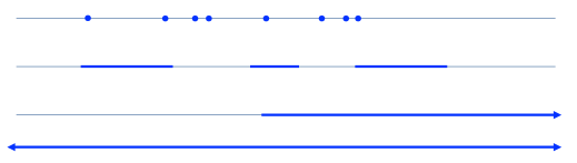
Figure 1: Examples of definable sets of $\mathbb{R}$.

O-minimal structures and definable sets: Let us give the full definition of an o-minimal structure. An o-minimal structure $\mathcal{S}$ is given by a collection $\mathcal{S}_{n}$ of subsets of $\mathbb{R}^{n}$ with $n\geq 1$ with the following properties

• The zero-set of any polynomial $P$ in $n$ variables is in $\mathcal{S}_{n}$;

• each $\mathcal{S}_{n}$ is closed under finite intersections, finite unions, and complements;

• if $A\in\mathcal{S}_{n}$ and $B\in\mathcal{S}_{m}$, then $A\times B\in\mathcal{S}_{n+m}$;

• if $\pi:\mathbb{R}^{n+1}\rightarrow\mathbb{R}^{n}$ is a linear projection and $A\in\mathcal{S}_{n+1}$, then $\pi(A)\in\mathcal{S}_{n}$;

• the set $\mathcal{S}_{1}$ consists of finite unions of points and intervals.

The elements of $\mathcal{S}_{n}$ are called the $\mathcal{S}$-definable sets of $\mathbb{R}^{n}$.

Definable maps: Having introduced the notion of an o-minimal structure, we can now define what we mean by a tame map in this setting. A map $f:A\rightarrow B$ between two $\mathcal{S}$-definable sets is called a $\mathcal{S}$-definable map if its graph is an $\mathcal{S}$-definable subset of $A\times B$. The notion of definable maps will be central in the following. For simplicity we will often drop the $\mathcal{S}$ and call the sets and maps to be definable. Some basic results for definable maps are: (1) the image and preimage of a definable set under a definable map is definable; (2) the composition of two definable maps is definable.

Definable topological spaces and manifolds: Given these definitions we can now proceed by defining an $\mathcal{S}$-definable topological space $M$. In order to do that one first introduces a definable atlas as a finite open covering $\{U_{i}\}$ of $M$ and a set of homeomorphisms $\phi_{i}:U_{i}\rightarrow V_{i}\subset\mathbb{R}^{n_{i}}$. Definability is imposed by requiring that (1) the $V_{i}$ and the pairwise intersections $\phi_{i}(U_{i}\cap U_{j})$ are definable sets, and (2) the transition functions are definable. Such a definable topological space can be upgraded to a $\mathcal{S}$-definable manifold $\mathcal{M}$ by requiring that the $V_{i}$ are open subsets of $\mathbb{R}^{n}$ and the transition functions are smooth. Complex definable manifolds are then obtained by viewing $\mathbb{C}^{n}\cong\mathbb{R}^{2n}$ and requiring the transition functions to be holomorphic. We can now develop this further and introduce definable subsets, definable morphisms, definable analytic spaces etc. The reader can consult [7] for further details. More important for the purpose of this work is to highlight in subsection 3.2 some of the implications that follow from imposing $\mathcal{S}$-definability. Before doing that it is crucial to give actual examples of o-minimal structures.

Examples of o-minimal structures: Note that there is no unique choice of o-minimal structure $\mathcal{S}$ of $\mathbb{R}^{n}$. The simplest example is the smallest structure that contains all the algebraic sets. It is given by collecting all semi-algebraic subsets of $\mathbb{R}^{n}$ and will be denoted by $\mathbb{R}_{\rm alg}$. These sets can be defined by polynomials $P(x_{1},...,x_{n})=0$ and polynomial inequalities $P(x_{1},...,x_{n})>0$, in $n$ variables, together with their finite unions. There are, however, various notable extensions of the smallest o-minimal structure $\mathbb{R}_{\rm alg}$ that are relevant in the following:

• An o-minimal structure, denoted by $\mathbb{R}_{\rm exp}$, is generated by $\mathbb{R}_{\rm alg}$ and the graph of the real exponential exp$:\mathbb{R}\rightarrow\mathbb{R}$ as shown in [8]. This implies that this structure is generated by all sets given by exponential polynomial equations $P(x_{1},...,x_{m},e^{x_{1}},...,e^{x_{m}})=0$ and projections thereof.

• An o-minimal structure, denoted by $\mathbb{R}_{\rm an}$, is generated by $\mathbb{R}_{\rm alg}$ extended by the graphs of all restricted real analytic functions. Such functions are all restrictions $f|_{B(R)}$ of functions $f$ that are real analytic on a ball $B(R^{\prime})$ of finite radius $R^{\prime}$ to a ball $B(R)$ of strictly smaller radius $R<R^{\prime}$.

• An o-minimal structure, denoted by $\mathbb{R}_{\rm an,exp}$, is generated by $\mathbb{R}_{\rm alg}$ extended by the graphs of the exponential function and all restricted real analytic functions.

Let us stress that it is a non-trivial task to find extensions of $\mathbb{R}_{\rm alg}$ that preserve o-minimality and Wilkie’s deep theorem that $\mathbb{R}_{\rm exp}$ is o-minimal is an example of this fact. However, it will be clear from the concrete applications to string theory effective actions that these extensions are crucially needed. In fact, we will see that we will be quickly led to use the o-minimal structure $\mathbb{R}_{\rm an,exp}$ as soon as exponential corrections, e.g. arising from instantons, play a role. For this reason the Tameness Conjecture is referring to $\mathbb{R}_{\rm an,exp}$.

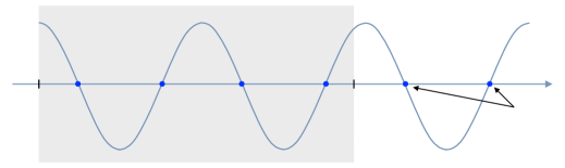
Figure 2: Graph of cosine function on $\mathbb{R}$ is non-definable set, but becomes definable when restricted to domain $0\leq\phi\leq a$.

Complex exponential function: To further highlight the relevance of $\mathbb{R}_{\rm an,exp}$, let us briefly discuss the complex exponential $e^{z}:\mathbb{C}\rightarrow\mathbb{C}$. Firstly, note that this function with domain $\mathbb{C}$ is never definable. This follows from the general fact that any definable and holomorphic function $f:\mathbb{C}^{n}\rightarrow\mathbb{C}$ has to be algebraic [7]. A more direct way to see that $e^{z}$ is never definable on $\mathbb{C}$ is to write $e^{z}=e^{r+i\phi}=e^{r}(\cos\phi+i\sin\phi)$. However, the graph of the sine- and cosine-functions on all of $\mathbb{R}$, cannot be definable, since the projection to the $\phi$-axis gives an infinite discrete set of zeros (see figure 2). To make $e^{z}$ definable, we first have to restrict the domain of $z$, say by demanding $0\leq\phi\leq a$. This resolves the issue of periodicity since $\cos(\phi)$ is definable in $\mathbb{R}_{\rm an}$, when restricting the domain if $\phi$. $e^{r}$ is, however, not in $\mathbb{R}_{\rm an}$ and we are thus lead to consider $\mathbb{R}_{\rm an,exp}$ to have a definable $e^{z}$ on the domain $0\leq\phi\leq a$.

Functions not definable in $\mathbb{R}_{\rm an,exp}$: As shown for the complex exponential, definability depends on the domain on which one considers a function. In the following we list a number of functions and domains, which have been shown in [44] to be not definable in $\mathbb{R}_{\rm an,exp}$. Firstly, we have the non-definability of the Gamma-function and Zeta-function

$$\Gamma(x)=\int_{0}^{\infty}e^{-t}t^{x-1}dt\ ,\qquad\zeta(x)=\sum_{n=1}^{\infty}\frac{1}{n^{x}}\ ,$$ (3.1)

when restricting the domain to $(0,\infty)$ and $(1,\infty)$, respectively. Secondly, also the error function $\int_{0}^{x}e^{-t^{2}}dt$ and the logarithmic integral $\int_{x}^{\infty}t^{-1}e^{-t}dt$ are not definable in $\mathbb{R}_{\rm an,exp}$ for $x\in\mathbb{R}$. It should be noted, however, that there can be cases in which an o-minimal structure exists that make these functions definable. This has been shown for $\Gamma(x)$, $\zeta(x)$ in [45].

3.2 On definable functions and the cell decomposition

In the following we want to summarize some basic results about $\mathcal{S}$-definable functions and $\mathcal{S}$-definable sets [7]. As above we will drop the symbol $\mathcal{S}$ if the statement is true for any o-minimal structure, but reintroduce it when making statements concerning a special structure.

Definable functions in one dimension: Let us begin by considering a definable function $f:(a,b)\rightarrow\mathbb{R}$. The open interval $(a,b)\subset\mathbb{R}$ can be of finite or infinite size, including the whole $\mathbb{R}$. Definability of $f$ implies [7] that $(a,b)$ admits a finite subdivision, i.e. a split

$$a=:a_{0}<a_{1}<...<a_{m-1}<a_{m}:=b\ ,$$ (3.2)

with the property that $f$ on the intervals $(a_{k},a_{k+1})$ is either constant or strictly monotonic and continuous. In particular, this implies that $f$ can only have finitely many discontinuities. One can even go one step further and show that there always exists a finite (possibly finer) decomposition of $(a,b)$, such that $f$ is once (or even multiple times) differentiable on the resulting open intervals. It also follows that $f$ can only admit finitely many minima and maxima. We depict a definable function in figure 3.

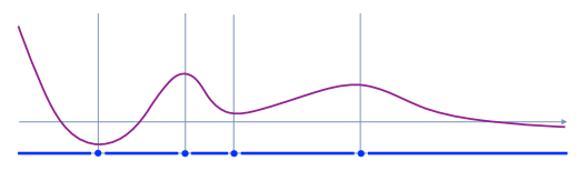
Figure 3: Sketch of the graph of a definable function from $\mathbb{R}\rightarrow\mathbb{R}$ and the split of the domain into finitely many open intervals.

Let us note that the notion of having a definable function has both local as well as global implications. To highlight one other implication let us now consider the o-minimal structure $\mathbb{R}_{\rm an,exp}$. If we consider a definable function in this o-minimal structure $f:\mathbb{R}\rightarrow\mathbb{R}$, we realize that for each such function there will be two infinitely long intervals $(-\infty,a_{1})$ and $(a_{m-1},\infty)$ along which the function is either constant or continuous and strictly monotonic. Since $\mathbb{R}_{\rm an,exp}$ only offers restricted analytic functions, they will actually not be relevant in some appropriately chosen subintervals $(-\infty,\tilde{a}_{1})$ and $(\tilde{a}_{m-1},\infty)$. This implies that in these ‘asymptotic regions’ of $\mathbb{R}$ the definable functions have either an algebraic or an exponential behavior.

Definable cylindrical cell decomposition: The use of the decomposition (3.2) of the interval $(a,b)$ hints towards a more general strategy that applies to dealing with definable sets and functions. More precisely, we will now introduce a definable cylindrical cell decomposition of $\mathbb{R}^{n}$. The following discussion might, at first, look rather technical and can be skipped in first reading. However, eventually the resulting description of definable sets is the base of many subsequent theorems in the study of o-minimal structures and gives an intuitive understanding about the properties of higher-dimensional definable sets and functions. To describe a definable cylindrical cell decomposition, we first note that it is a partition of $\mathbb{R}^{n}=\cup_{i}D_{i}$ into finitely many pairwise disjoint definable subsets $D_{i}$, which are called cells. The crucial part is that these cells have special inductive description:

• For $n=0$, i.e. $\mathbb{R}^{0}$, there is a unique cell, which is simply all of $\mathbb{R}^{0}$, i.e. a point.

• For $n=1$, i.e. $\mathbb{R}$, the cells are obtained by a decomposition (3.2) of the interval $(-\infty,\infty)$. They consist of the points $\{a_{k}\}$ for $0<k<m$, and the open intervals $(a_{k},a_{k+1})$ for $0\leq k<m$. We depict such a decomposition in figure 4.

  

  Figure 4: A definable cylindrical cell decomposition of $\mathbb{R}$.

• In general, for $n>0$, we write $\mathbb{R}^{n}=\mathbb{R}^{n-1}\times\mathbb{R}$. Now we can assume that we have a definable cylindrical cell decomposition $\{\mathcal{D}_{\alpha}\}$ for $\mathbb{R}^{n-1}$. For each cell $\mathcal{D}_{\alpha}$ we now have an integer $m_{\alpha}>0$ and definable continuous functions $f^{(\alpha)}_{k}:\mathcal{D}_{\alpha}\rightarrow\mathbb{R}$ for $0<k<m_{\alpha}$ such that

  $$-\infty=:f^{(\alpha)}_{0}<f^{(\alpha)}_{1}<\ldots<f^{(\alpha)}_{m_{\alpha}-1}<f^{(\alpha)}_{m_{\alpha}}:=\infty\ ,$$ (3.3)

  where the inequalities are meant to hold on all of $\mathcal{D}_{\alpha}$. Having such a set of functions the cells in $\mathbb{R}^{n}$ are:
  (1) graphs of the functions, i.e. $\{(x,f^{(\alpha)}_{k}(x))\subset\mathbb{R}^{n}:x\in\mathcal{D}_{\alpha}\}$ for each $\mathcal{D}_{\alpha}$;
  (2) bands between the functions, i.e. $\{(x,y)\subset\mathbb{R}^{n}:x\in\mathcal{D}_{\alpha},\text{ $y$ in interval}\ (f^{(\alpha)}_{k}(x),f^{(\alpha)}_{k+1}(x))\}$.

Due to its iterative nature, the definition of a definable cylindrical cell decomposition uses an ordering of the coordinates. The arising cells are thus admitting special directions along which there is a simple projection to a low-dimensional cell decomposition. We illustrate this in figure 5, where we depict a definable cylindrical cell decomposition of $\mathbb{R}^{2}$ build from the decomposition of $\mathbb{R}$ depicted in figure 4.

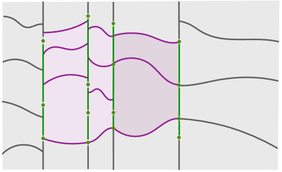
Figure 5: A definable cylindrical cell decomposition of $\mathbb{R}^{2}$ build from the decomposition in figure 4. The new $\mathbb{R}^{2}$-cells are graphs and bands of definable functions on the $\mathbb{R}$-cells. The new cells over the open intervals $(a_{1},a_{2})$, …, $(a_{3},a_{4})$ are shown in purple, while the new cells over the points $a_{1},...,a_{4}$ are shown in green. We have coloured all cells stretching to $\pm\infty$ in grey.

Cell decomposition theorem: The remarkable fact about the cell decomposition is that they are sufficient to describe any definable set. In fact, one can show the cell decomposition theorem: (1) Given any finite collection of definable sets $A_{1},...,A_{k}\in\mathbb{R}^{n}$ there is a definable cylindrical cell decomposition such that each $A_{i}$ is a finite union of cells; (2) For each definable function $f:A\rightarrow\mathbb{R}$, $A\subset\mathbb{R}^{n}$ there is a cylindrical cell decomposition of $\mathbb{R}^{n}$ such that partitions $A$ as in (1) in such a way that $f$ restricted to each cell is continuous. This theorem can be further refined by replacing the requirement of having continuous functions in the definition of the cells by having functions that are once (or multiple times) differentiable. In this case the cells might be smaller, but the cell decomposition theorem still holds.

Dimension and Euler characteristic: The cell decomposition theorem has many applications. For example, it can be used to show that one can associate a dimension and an Euler characteristic to each definable set. Let us consider a definable set $A$ and denote by $\mathcal{D}_{i}$ the finite number of cells in which it can be partitioned using the cell decomposition theorem. The dimension $\text{dim}(A)$ of $A$ is simply defined to be maximum found for the dimensions $\text{dim}(\mathcal{D}_{i})$ of the cells $\mathcal{D}_{i}$. The Euler characteristic is defined to be

$$E(A)=\sum_{\mathcal{D}_{i}}(-1)^{\text{dim}(\mathcal{D}_{i})}=k_{0}-k_{1}+...+(-1)^{\text{dim}(A)}k_{\text{dim}(A)}\ ,$$ (3.4)

where $k_{s}$ is the number of $s$-dimensional cells in $\{\mathcal{D}_{i}\}$. Crucially, the values of $\text{dim}(A)$ and $E(A)$ are independent of the chosen cell decomposition and hence can serve as invariants associated to the definable set $A$.

Definable family and uniform boundedness: In the concrete applications to effective theories, the notion of having a definable family of sets will be useful. To define such a family we consider a definable set $S\subset\mathbb{R}^{m+n}=\mathbb{R}^{m}\times\mathbb{R}^{n}$. We then introduce the subsets $S_{\lambda}\subset\mathbb{R}^{n}$ by setting

$$S_{\lambda}=\{x\in\mathbb{R}^{n}:(\lambda,x)\in S\}\ .$$ (3.5)

The sets $S_{\lambda}$ are the fibers of the definable family $\{S_{\lambda}\}_{\lambda\in\mathbb{R}^{m}}$. Note that the definable family is defined over all of $\mathbb{R}^{m}$, but will have empty fibers at points that do not lie in the projection of $S$ to $\mathbb{R}^{m}$. The cell decomposition theorem can now be used to prove uniform boundedness results for definable families. For example, consider a definable family $S_{\lambda}$. Then there exists a positive integer $m$, such that $S_{\lambda}$ has at most $m$ isolated points. In particular, each fiber containing only a finite number of points has at most $m$ such points.

Definability in an o-minimal structure has found numerous applications in geometry. In particular, it is interesting to point out that ‘definability’ has been used in various theorems as a replacement of stronger properties of geometric spaces in algebraic geometry. To quote two influential theorems in which definability replaces compactness, let us mention the definable Chow theorem [46] and the Pila-Wilkie theorem [47].

This ends our brief account on o-minimal structures and tame geometry. It is important to stress that this is a broad and well-developed field and the preceding summary should be seen more as an invitation to the field rather than aiming at giving a complete account.

4 Tame geometry of the string landscape

In this section we discuss the evidence for the validity of the Tameness Conjecture. Before doing so, we want to use the mathematical background introduced in section 3 to elaborate on the statement of the conjecture itself.

The Tameness Conjecture makes the assertion that the allowed parameter spaces, scalar field spaces, and coupling functions are definable in an o-minimal structure. While at first this statement deals with very different objects, we now realize from subsection 3.1 that we should understand the parameter space $\mathcal{P}$, and the field spaces $\mathcal{M}_{\lambda}$ as subsets of $\mathbb{R}^{n}$ and $\mathbb{R}^{m}$ for sufficiently large $n$ and $m$, respectively. The coupling functions we then understand as maps from these subsets into suitable target spaces that are also embedded into some real Euclidean ambient space. As discussed in the beginning of section 2 the field space $\mathcal{M}_{\lambda}$ can depend on the parameters chosen from $\mathcal{P}$ and, therefore, should be understood as being part of the combined set $\mathcal{D}$ defined in (2.2), which has fibers $\mathcal{M}_{\lambda}$. The definability statement now asserts that the set $\mathcal{D}$, understood as a subset of $\mathbb{R}^{m+n}$, is a definable set in some o-minimal structure. We can also use the notion of definable family introduced in subsection 3.2, see (3.5). The Tameness Conjecture then implies the statement:

The scalar field spaces $$\{\mathcal{M}_{\lambda}\}_{\lambda\in\mathbb{R}^{n}} \mathcal{M}_{\lambda}=\emptyset \lambda\notin\mathcal{P}$$ form a definable family, where if . (4.1)

If $\mathcal{M}_{\lambda}$ would be merely a set, a non-trivial consequence of definability is the fact that there is a well-defined $\text{dim}(\mathcal{M}_{\lambda})$ with $\text{dim}(\mathcal{M}_{\lambda})\leq n$ for all $\lambda$. This fits with our assertion that $\mathcal{M}_{\lambda}$ has more structure, since it is considered to be the field space of some scalars $\phi^{i}$. In particular, we want to endow $\mathcal{M}_{\lambda}$ with a metric to define the kinetic terms of $\phi^{i}$. Hence, we require $\mathcal{M}_{\lambda}$ to be a Riemannian manifold. The definability statement then amounts to the statement that $\mathcal{M}_{\lambda}$ is a definable manifold with a definable metric $g:T\mathcal{M}_{\lambda}\times T\mathcal{M}_{\lambda}\rightarrow\mathbb{R}$. The statement (4.1) can then be strengthened to: $\{\mathcal{M}_{\lambda}\}_{\lambda\in\mathbb{R}^{n}}$ forms a definable family of Riemannian manifolds. We similarly proceed for the other coupling functions in the effective theory. If a coupling function admits some additional property, the Tameness Conjecture asserts that definability in an o-minimal structure should arise as an additional and compatible feature.

In the remainder of this section we provide evidence for the Tameness Conjecture by going through the various compactifications mentioned in section 2 and introduce some recent mathematical results that confirm definability in the o-minimal structure $\mathbb{R}_{\rm an,exp}$. In subsection 4.1 we comment on string theory effective actions with 8 or more supercharges and exploit the fact that arithmetic quotients are definable manifolds and that period mappings are definable maps. In subsection 4.2 we sketch the proof that also the Type IIB/F-theory flux landscape is definable.

4.1 Effective theories with extended supersymmetry

In order to provide evidence for the Tameness Conjecture we will first comment on the higher-supersymmetric settings and then turn to Calabi-Yau threefold compactifications with $\mathcal{N}=2$ supersymmetry. The settings that we are going to discuss have been already introduced in subsection 2.1.

Definability in higher-supersymmetric settings. In theories with more than 8 supercharges we recalled that the moduli spaces are arithmetic quotients (2.3). Fixing the groups $G,K$ and the lattice $\Gamma$, it is a central result of Bakker, Klingler, Tsimerman [23] that the manifolds $\mathcal{M}_{\Gamma,G,K}=\Gamma\backslash G/K$ are definable in the o-minimal structure $\mathbb{R}_{\rm alg}$. Remarkably, the definable structure of $\mathcal{M}_{\Gamma,G,K}$ is inherited from the natural definable structure of $G/K$. This implies that the field spaces for these theories are definable also in $\mathbb{R}_{\rm an,exp}$ containing $\mathbb{R}_{\rm alg}$. Furthermore, it should then be not too hard to check that also the coupling functions varying over $\mathcal{M}_{\Gamma,G,K}$ are definable in $\mathbb{R}_{\rm alg}$ due to the fact that they are given by polynomial expressions.

More subtle is the question if $\mathcal{M}_{\Gamma,G,K}$ and the coupling functions are also definable when considered jointly with the parameter space $\mathcal{P}$. Note that in general there are infinitely many choices for the groups $(G,K,\Gamma)$. Each choice we consider as being labelled by a discrete parameter in the space $\mathcal{P}$. Whether or not the allowed set is finite is, at least in some of the settings, still an open question. For example, consider a six-dimensional effective theory with $\mathcal{N}=(1,0)$ supersymmetry. This theory has 8 supercharges, but the scalar field space in the tensor and vector sector of the theory is still an arithmetic quotient with $G=SO(1,T)$, where $T$ is the number of tensor multiplets. Bounds on $T$ and general finiteness statements about such six-dimensional theories were recently discussed in [22]. Evidence in this direction can therefore be directly interpreted as evidence for the Tameness Conjecture. Conversely, assuming the Tameness Conjecture a finiteness constraint on $T$ is a necessary criterion, since infinite discrete sets are never definable.

Definability in Calabi-Yau threefold compactifications with $\mathcal{N}=2$. Let us now turn to the four-dimensional supergravity theory with $\mathcal{N}=2$ supersymmetry, i.e. 8 supercharges, that arise when compactifying Type IIB string theory on a Calabi-Yau threefold. We have introduced some basics on these settings already in subsection 2.1. Recall that supersymmetry implies that the field space spanned by the complex scalars in the vector multiplets is a special Kähler manifold $\mathcal{M}_{\rm cs}$. The relevant local metric $g_{i\bar{\jmath}}$ on this manifold takes the form (2.5), while the gauge coupling functions $f_{AB}$ for the vector fields was given in (2.6). Both can be expressed in terms of the periods $\Pi$ of the $(3,0)$-form $\Omega$ introduced in (2.4). Note that supersymmetry already implies that $g_{i\bar{\jmath}}$ and $f_{AB}$ can be expressed in terms of a holomorphic function $\Pi$, but there are no general constraints on $\Pi$ that go beyond the special geometry relations (see, e.g. [48], for an introduction to this subject). In Calabi-Yau compactifications $\Pi$ is much more constrained, since it arises from a so-called period mapping. In fact, it is a very remarkable result of Bakker, Klingler, and Tsimerman [23] that the period mappings are definable in $\mathbb{R}_{\rm an,exp}$.

To introduce the precise statement we first recall some facts about $\mathcal{M}_{\rm cs}$ and then explain the notion of a period mapping. In preparation for the discussion of the scalar potential in subsection 4.2 we will present the following discussion for a general Calabi-Yau manifold of complex dimension $D$. For a polarized Calabi-Yau $D$-fold the moduli space $\mathcal{M}_{\rm cs}$ is complex quasi-projective [36] and smooth after possibly performing a resolution [49]. We can view $\mathcal{M}_{\rm cs}$ as an $\mathbb{R}_{\rm an,exp}$-definable manifold by extending its $\mathbb{R}_{\rm alg}$-definable manifold structure. To introduce the period mapping, our starting point is the Hodge decomposition of the middle cohomology of $Y_{D}$. Let us thus consider the decomposition

$$\mathcal{H}_{\mathbb{C}}=\bigoplus_{p+q=D}H^{p,q}\ ,$$ (4.2)

where $\mathcal{H}_{\mathbb{C}}$ is the primitive part of the middle cohomology $\mathcal{H}_{\mathbb{C}}=H^{D}_{\rm prim}(Y_{D},\mathbb{C})$, i.e. we impose $J\wedge\omega=0$ for $\omega\in\mathcal{H}_{\mathbb{C}}$ and $J$ being a Kähler form on $Y_{D}$. Note that $H^{3}_{\rm prim}(Y_{3})=H^{3}(Y_{3})$, if we require that $H^{1}(Y_{3})$ vanishes. Importantly, the decomposition (4.2) depends on the point in $\mathcal{M}_{\rm cs}$ at which it is evaluated. The period map $h$, which in turn determines the period integrals, encodes this dependence by expressing the relation of the $H^{p,q}$ at some point $z$ with respect to a reference point $H^{p,q}_{\rm ref}$. Concretely, let us define $h$ as

$$H^{p,q}=h(z,\bar{z})H^{p,q}_{\rm ref}\ ,$$ (4.3)

where $h$ can be represented by a matrix acting on fixed basis of $\mathcal{H}_{\mathbb{C}}$. This allows us to identify the period integrals

$$\Pi=\int_{\gamma_{I}}h\Omega_{\rm ref}\ ,$$ (4.4)

where $\Omega_{\rm ref}$ is representing the one-dimensional space $H^{D,0}_{\rm ref}$. We note that $h$ becomes holomorphic when evaluated on a suitable basis $F^{p}_{\rm ref}=\bigoplus_{k=p}^{D}H^{k,D-k}$.

The map $h$ can be understood as maps into arithmetic quotients of the form (2.3). To see this, we first introduce two real groups $V\subset G\subset\text{Gl}(\mathcal{H}_{\mathbb{R}})$. To define $G$, we first introduce on $\mathcal{H}_{\mathbb{C}}$ the bilinear form

$$(a,b)\equiv\int_{Y_{D}}a\wedge b\ ,$$ (4.5)

where $a,b\in\mathcal{H}_{\mathbb{C}}$. The group $G$ consist of all elements in $\text{Gl}(\mathcal{H}_{\mathbb{R}})$ that preserve this bilinear form, i.e. obey $(ga,gb)=(a,b)$. A subgroup of $G$, denoted by $V$, is the group of elements that additionally preserve the whole reference $(p,q)$-splitting, i.e. obey $vH^{p,q}_{\rm ref}=H^{p,q}_{\rm ref}$. Up to global symmetries, which we will discuss in a moment, one can use these groups to identify $h$ as a map $h:\mathcal{M}_{\rm cs}\rightarrow G/V$. In order to discuss the global symmetries, note that $\mathcal{M}_{\rm cs}$ is not simply connected. The monodromy group $\Gamma$, being a representation of the fundamental group of $\mathcal{M}_{\rm cs}$ on $\mathcal{H}_{\mathbb{Z}}=\mathcal{H}_{\mathbb{C}}\cap H^{D}(M,\mathbb{Z})$, captures the information about the non-trivial fibration structure of the Hodge decomposition $H^{p,q}$ arising due to this fact. Hence, $h$ should actually be viewed as a map

$$h:\ \mathcal{M}_{\rm cs}\rightarrow\Gamma\backslash G/V.$$ (4.6)

A foundational result of Bakker, Klingler, Tsimerman [23] is the theorem:

$$\boxed{\rule[-2.84544pt]{0.0pt}{14.22636pt}\quad\text{The period mapping $h$ is definable in the o-minimal structure}\ \mathbb{R}_{\rm an,exp}\ .\quad}$$ (4.7)

While we will not aim at reviewing the details of the proof of this statement, a few remarks might help to illuminate the steps that go into the argument. Firstly, as mentioned above, $h$ can be viewed as a holomorphic map, just like $\Pi$. The essential part of the proof is then to control the asymptotic behavior near the boundaries of $\mathcal{M}_{\rm cs}$, since we can ‘discard’ the compact region making up the interior of the moduli space. This is due to the fact that $\mathbb{R}_{\rm an,exp}$-definable functions include any restricted analytic function, which endows us with a sufficiently large set of choices for this compact region. The fact that the asymptotic form of $h$ is constrained as shown by Schmid [37], see (2.7) for the analog statement for $\Pi$, suffices to establish that $h$ is compatible with $\mathbb{R}_{\rm an,exp}$-definability at least before modding out by $\Gamma$. To show that the quotient by $\Gamma$ does not ruin definability is more involved and requires to use another important result of asymptotic Hodge theory, namely the sl(2)-orbit theorem [37, 50].

We are now in the position to discuss the validity of the Tameness Conjecture in these $\mathcal{N}=2$ settings using the fact (4.7). Since the periods $\Pi$ are given by (4.4) they are also definable in $\mathbb{R}_{\rm an,exp}$. This fact can now be used in the expressions (2.5) and (2.6) for the field space metric $g_{i\bar{\jmath}}$ and the gauge coupling functions $f_{\alpha\beta}$ to establish their definability in $\mathbb{R}_{\rm an,exp}$ over $\mathcal{M}_{\rm cs}$. Hence, we have assembled another non-trivial piece of evidence for the Tameness Conjecture. Let us stress that our analysis only establishes definability over the moduli space $\mathcal{M}_{\rm cs}$. It is well-known that the periods $\Pi$ also depend on parameters that are fixed in terms of the geometric data of $Y_{D}$. For example, $\Pi$ near the large complex structure point in $\mathcal{M}_{\rm cs}$ depends on the topological data of the mirror Calabi-Yau manifold associated to $Y_{D}$, such as its intersection numbers and Chern classes. The parameter space $\mathcal{P}$ therefore contains a discrete set of data and definability would be lost if this set is infinite. In particular, it is a consequence of the Tameness Conjecture that the number of topologically distinct compact Calabi-Yau manifolds is finite (see [51] for a more precise notion of distinguishing Calabi-Yau manifolds). Establishing this finiteness statement would thus be a central test of the Tameness Conjecture. While we will not be able to address finiteness of geometries, the next subsection will be devoted to establishing a non-trivial definability result over another discrete parameter space, namely a flux lattice.

4.2 Definability of the flux landscape

In this subsection we discuss a definability statement that establishes the Tameness Conjecture being satisfied over a discrete parameter space. More precisely, we will study flux compactifications introduced in subsection 2.2 and show that the scalar potential as a function of the complex structure deformations and the flux parameters is definable close to its self-dual vacuum locus (2.13). We will summarize the proof of this statement by following the work of Bakker, Schnell, Tsimerman, and the author [27]. For simplicity, we restrict the following arguments to a study of $G_{4}$ flux on a Calabi-Yau fourfold that yields a scalar potential (2.12).

To begin with, we introduce in addition to (4.5) a second bi-linear form on $\mathcal{H}_{\mathbb{C}}=H^{4}_{\rm prim}(Y_{4},\mathbb{C})$ which is associated with the Hodge norm by setting

$$\qquad\langle a|b\rangle\equiv(\bar{a},Cb)=\int_{Y_{D}}\bar{a}\wedge\star b\ ,$$ (4.8)

and we denote $\|a\|^{2}=\langle a|a\rangle$ as in (2.10). Here we have introduced the Weil operator $C$, which is nothing else than the Hodge star acting on elements of the cohomology. Note that $C$ acts on elements in $H^{p,q}$ with an eigenvalue $(-1)^{\frac{1}{2}(p-q)}$ and hence satisfies $C^{2}=1$ for even $D$ and $C^{2}=-1$ for odd $D$. Just as the periods $\Pi$ and the period mapping $h$, also $C$ will vary over the complex structure moduli space $\mathcal{M}_{\rm cs}$. To describe this behavior we again fix a reference Hodge decomposition $H^{p,q}_{\rm ref}$ and an associated Weil operator $C_{\rm ref}$. The Weil operator at the point $z$ in $\mathcal{M}_{\rm cs}$ can be obtained from $C_{\rm ref}$ by using the period mapping introduced in the previous section by

$$C(z,\bar{z})=h^{-1}C_{\rm ref}h$$ (4.9)

but it turns out to be better to consider $C(z,\bar{z})$ directly and study its properties as a map from $\mathcal{M}_{\rm cs}$ into some quotient space. To find this quotient we note that every Weil operator $C^{\prime}$ can be obtained from $C_{\rm ref}$ by acting with an element $g\in G$ as $C^{\prime}=gC_{\rm ref}g^{-1}$. For later use, let us denote this operator by

$$C_{g}:=gC_{\rm ref}g^{-1}\ .$$ (4.10)

Denoting by $K$ the group elements preserving $C_{\rm ref}$ we thus identify $C$ as a map

$$C:\mathcal{M}_{\rm cs}\rightarrow G/K\ .$$ (4.11)

Here the symmetric space $G/K$ labels all inequivalent Weil operators that can be defined on $\mathcal{H}_{\mathbb{C}}$.

Scalar potential for fixed flux. Let us now turn to the analysis of the flux scalar potential. As a first step, we will fix the flux $G_{4}$ and only consider the dependence on $\mathcal{M}_{\rm cs}$. In this case the argument for $V$ being definable in $\mathbb{R}_{\rm an,exp}$ is analog to the analysis of the field space metric and gauge coupling function outlined in subsection 4.1. Recall that the Hodge star in (2.12) reduces to $C$ on cohomology classes, and hence we can write in the notation of this section

$$V(z,v)=c\|Cv-v\|^{2}\ .$$ (4.12)

As we move along $\mathcal{M}_{\rm cs}$ the Hodge decomposition will vary and hence also the associated Weil operator. It now follows from (4.9) and the definability of the period map (4.7) that

$$\boxed{\rule[-2.84544pt]{0.0pt}{12.80365pt}\quad\text{The Weil operator $C$ is definable in the o-minimal structure}\ \mathbb{R}_{\rm an,exp}\ .\quad}$$ (4.13)

Since $\|\cdot\|$ is built using $C$, we readily apply (4.30) to conclude that

$$V(G_{4}):\ \mathcal{M}_{\rm cs}\rightarrow\mathbb{R}\ \ \text{is}\ \ \mathbb{R}_{\rm an,exp}\text{-definable}\ .$$ (4.14)

By a generalization of the statements of subsection 3.2 one sees that it therefore has only finitely many disconnected sets of zeros and minima. Note that this is also true if we replace $V$ with any definable function of $C$.

It is important to stress at this point that the statement (4.14) only holds when fixing the flux $G_{4}$. Since, $G_{4}$ takes values on a lattice, definability as a function of the parameter $G_{4}$ will be lost if no further constraints are imposed on $G_{4}$. It is not hard to see that also the tadpole constraint $(G_{4},G_{4})=\ell$ still allows for infinitely many choices of $G_{4}$ and hence does not suffice to ensure definability. In the next step we will see, however, that $V$ as a function of $G_{4}$ is actually definable near self-dual vacua when imposing the tadpole constraint.

Definability and self-dual fluxes. Let us now also take into account that one can choose the fluxes $G_{4}$ in the scalar potential from a lattice $\mathcal{H}_{\mathbb{Z}}=H^{4}(Y_{4},\mathbb{Z})\cap H^{4}_{\rm prim}(Y_{4},\mathbb{R})$ as long as they satisfy the tadpole constraint. We sketch the proof that definability is retained in the product of $\mathcal{M}_{\rm cs}$ and the flux lattice when considering the zeros of $V(v,z)$ given in (4.12). More precisely, let us introduce the Hodge bundle $E$ with fibers $\mathcal{H}_{\mathbb{C}}$, which encodes the variation of the $(p,q)$-decomposition of $\mathcal{H}_{\mathbb{C}}$ when moving over the base $\mathcal{M}_{\rm cs}$. Note that $E$ is an algebraic bundle and hence is a definable manifold in $\mathbb{R}_{\rm alg}\subset\mathbb{R}_{\rm an,exp}$. Our aim is to study the subsets of $E$ at which the integral fluxes in the fibers of $E$ satisfy the self-duality and the tadpole condition. The statement proved in [27] is

$$\boxed{\rule[-11.38092pt]{0.0pt}{31.2982pt}\quad\begin{array}[]{l}\text{The subset $\{(z,G_{4})\subset E$ with fluxes $G_{4}$ s.t.~{}$C(z)G_{4}=G_{4},(G_{4},G_{4})=\ell\}$ }\\[2.84544pt] \text{is definable in the o-minimal structure}\ \mathbb{R}_{\rm an,exp}\ .\end{array}\quad}$$ (4.15)

In particular, this includes the observation that a reduction of $E$ to this set has finite fibers. Using the statements about definable families and uniform boundedness from subsection 3.2 one thus concludes that there are only finitely many fluxes $G_{4}$ that possibly can satisfy the self-duality and tadpole conditions.

To elucidate some of the steps that go into showing (4.15), let us fix a $\mathcal{H}_{\mathbb{Z}}$ not changing over $\mathcal{M}_{\rm cs}$ and note the all integral elements in $E$ can be reached from this $\mathcal{H}_{\mathbb{Z}}$ up to monodromy. Hence we want to study the sets

$$(\mathcal{M}_{\alpha},G^{\alpha}_{4})\subset\mathcal{M}_{\rm cs}\times\mathcal{H}_{\mathbb{Z}}\ ,\qquad{\alpha=1,2,...}\ ,$$ (4.16)

by requiring

$$(1) (G_{4}^{\alpha},G_{4}^{\alpha})=\ell\ ,$$ (4.17)

$$(2) C(z,\bar{z})G_{4}^{\alpha}=G_{4}^{\alpha}\quad\forall z\in\mathcal{M}_{\alpha}\ ,$$ (4.18)

where no sum over $\alpha$ needs to be performed in $(1)$. To obtain these sets, we pick a flux $G^{\alpha}$ satisfying (1) and then determine all points in $\mathcal{M}_{\rm cs}$ that are obeying (2). At first, since there infinitely many choices for $G^{\alpha}_{4}\in\mathcal{H}_{\mathbb{Z}}$, the index range of $\alpha$ is infinite. Furthermore, also $\mathcal{M}_{\alpha}$ could have infinitely many disconnected components. For the second statement, however, definability of $C$ as stated in (4.30) actually ensures that $\mathcal{M}_{\alpha}$ is $\mathbb{R}_{\rm an,exp}$-definable, and hence has only finitely many connected components. We now want to show that the index range of $\alpha$ is actually finite.

Let us introduce the symmetry group $\Gamma_{\mathcal{H}}$ of the lattice $\mathcal{H}_{\mathbb{Z}}$ preserving the inner product by setting

$$\Gamma_{\mathcal{H}}=O(\mathcal{H}_{\mathbb{Z}},(\cdot,\cdot))\ ,$$ (4.19)

An important step in [27] is to use this symmetry group and reduce the lattice into finitely many orbits of $\Gamma_{\mathcal{H}}$ along which we then are able to show definability. To do that we use a result of Kneser [52] on lattices and bilinear forms. Let us pick a $G_{4}\in\mathcal{H}_{\mathbb{Z}}$ and act with all elements in $\Gamma_{\mathcal{H}}$ on $G_{4}$ to define the equivalence class $[G_{4}]$. Kneser now shows that the set of fluxes $G_{4}$ with a fixed $(G_{4},G_{4})=\ell$ is obtained from only finitely many such classes. In other words, one can select finitely many fluxes

$$G_{4}^{A}\ ,\quad A=1,...,n\ :\qquad(G^{A}_{4},G^{A}_{4})=\ell\ ,$$ (4.20)

and generate the whole set of solutions to $(G_{4},G_{4})=\ell$ by acting with $\Gamma_{\mathcal{H}}$. Remarkably, the tadpole condition thus gives us a reduction to checking definability in finitely many orbits $\Gamma_{\mathcal{H}}G_{4}^{A}$.

Let us fix a reference Weil operator $C_{\rm ref}$ as in (4.9) and pick one flux $F\in\mathcal{H}_{\mathbb{Z}}$ that obeys $(F,F)=\ell$ and is self-dual with respect to $C_{\rm ref}$, $C_{\rm ref}F=F$. Clearly, $F$ can be taken to be one of the $G_{4}^{A}$ in (4.20) from which we generate a $\Gamma_{\mathcal{H}}$-orbit. We now want to consider all $C_{g}$ introduced in (4.10) that preserve self-duality of $F$, i.e. we will look at the set

$$\big{\{}(gK,F):\ C_{g}F=F\big{\}}_{g\in G}\ \subset\ G/K\times\mathcal{H}_{\mathbb{Z}}\ ,$$ (4.21)

where we recall that each set $gK$ represents a Weil operator via (4.10), since $K$ preserves $C_{\rm ref}$. Looking at sets (4.21) is analogous to (4.16), but we now work with sets representing Weil operators instead of subsets of $\mathcal{M}_{\rm cs}$. It will be the final key step to ensure that going from $\mathcal{M}_{\rm cs}$ to Weil operators can be done in an $\mathbb{R}_{\rm an,exp}$-definable way. We note that the equations $C_{g}F=F$ and $(F,F)=\ell$ have the symmetry

$$C_{g}\rightarrow kC_{g}k^{-1}\ ,\qquad F\rightarrow kF\ ,\qquad k\in\Gamma_{\mathcal{H}}\ .$$ (4.22)

Hence, it will suffice the think about the set $\Gamma_{\mathcal{H}}(gK,F)$, where the action of the group $\Gamma_{\mathcal{H}}$ is via $\alpha(gK,F)=(\alpha gK,\alpha F)$, and work on the quotient

$$\Gamma_{\mathcal{H}}\backslash(G/K\times\mathcal{H}_{\mathbb{Z}})\ .$$ (4.23)

Let us now consider the orbit $\Gamma_{\mathcal{H}}F\subset\mathcal{H}_{\mathbb{Z}}$ generated when acting with all elements of $\Gamma_{\mathcal{H}}$ on $F$. To begin with, we define the real groups $G_{F},K_{F},\Gamma_{F}$ as the subgroups preserving $F$, i.e. we set

$$G_{F}=\{h\in G:hF=F\}\ ,\qquad K_{F}=K\cap G_{F}\ ,\qquad\Gamma_{F}=\Gamma_{\mathcal{H}}\cap G_{F}\ .$$ (4.24)

Since $F$ is self-dual with respect to $C_{\rm ref}$ it is an element in $G_{F}/K_{F}$. In fact, the symmetric space $G_{F}/K_{F}$ labels all Weil operators $C_{g}$ that fix the element $F$. We now consider a $F_{\gamma}=\gamma F\in\Gamma_{\mathbb{Z}}F$ that is also self-dual with respect to $C_{g}$. This implies that we can write

$$F=\gamma^{-1}F_{\gamma}=\gamma^{-1}C_{g}F_{\gamma}=\gamma^{-1}C_{g}\gamma F=C_{\gamma^{-1}g}F\ .$$ (4.25)

Since $C_{\gamma^{-1}g}$ is a Weil operator fixing $F$ there should be an $h\in G_{F}$ such that $C_{h}=C_{\gamma^{-1}g}$. Reading this as the condition $C_{\rm ref}=C_{h^{-1}\gamma^{-1}g}$ we conclude that $h^{-1}\gamma^{-1}g\in K$. This implies that

$$\Gamma_{\mathcal{H}}(gK,F_{\gamma})=\Gamma_{\mathcal{H}}(hK,F)\ .$$ (4.26)

This relation implies that the set of $\{F_{\gamma}\}_{\gamma\in\Gamma_{\mathcal{H}}}$ with $C_{g}F_{\gamma}=F_{\gamma}$ is actually the image of a map

$$i:\Gamma_{F}\backslash G_{F}/K_{F}\rightarrow\Gamma_{\mathcal{H}}\backslash(G/K\times\mathcal{H}_{\mathbb{Z}})\ ,\qquad\Gamma_{F}hK_{F}\mapsto\Gamma_{\mathcal{H}}(hK,F)\ .$$ (4.27)

However, by of another result of [23] (see also [27]), such maps between algebraic quotients are actually $\mathbb{R}_{\rm alg}$-definable. The locus of Weil operators mod $\Gamma_{\mathcal{H}}$ and self-dual classes in $\Gamma_{\mathcal{H}}F$, i.e.

$$\big{\{}\ \Gamma_{\mathcal{H}}(gK,F_{\gamma}):\ C_{g}F_{\gamma}=F_{\gamma}\ \big{\}}_{g\in G,\gamma\in\Gamma_{\mathcal{H}}}\ \subset\ \Gamma_{\mathcal{H}}\backslash(G/K\times\mathcal{H}_{\mathbb{Z}})$$ (4.28)

is therefore an $\mathbb{R}_{\rm alg}$-definable subset that is isomorphic to the smaller arithmetic quotient $\Gamma_{F}\backslash G_{F}/K_{F}$.

It remains to show that definability of the set (4.28) in $\Gamma_{\mathcal{H}}\backslash(G/K\times\mathcal{H}_{\mathbb{Z}})$ can be carried over to the space $\mathcal{M}_{\rm cs}\times\mathcal{H}_{\mathbb{Z}}$. This actually follows from an extension of the definability property of the Weil operator (4.30). In fact, in order to show the definability of the period mapping (4.7), the authors of [23] actually first prove the definability of $C$ mod $\Gamma_{\mathcal{H}}$. Let us define the Weil operator period map

$$[C]:\ \mathcal{M}_{\rm cs}\rightarrow\Gamma_{\mathcal{H}}\backslash G/K\ ,$$ (4.29)

which associates to each point in $\mathcal{M}_{\rm cs}$ its Weil operator modulo $\Gamma_{\mathcal{H}}$. The definability statement then reads [23]

$$\boxed{\rule[-2.84544pt]{0.0pt}{12.80365pt}\quad\text{The Weil operator period map $[C]$ is definable in the o-minimal structure}\ \mathbb{R}_{\rm an,exp}\ .\quad}$$ (4.30)

We stress that this is a stronger statement than the definability of the period mapping stated in (4.7), since the latter involves the monodromy group $\Gamma$ and $\Gamma\subset\Gamma_{\mathcal{H}}$. Finally, one has to extend the map (4.29) to an $\mathbb{R}_{\rm an,exp}$-definable map $E\rightarrow\Gamma_{\mathcal{H}}\backslash(G/K\times\mathcal{H}_{\mathbb{Z}})$. This is straightforward if one thinks about $E$ being the product $\mathcal{M}_{\rm cs}\times\mathcal{H}_{\mathbb{C}}$, but requires some extra work to incorporate the bundle structure in a definable way as explained in [27, 53]. Since the pre-image of the sets (4.28) are precisely the self-dual integral classes satisfying the tadpole constraint, and a definable set under a definable map is definable, we can conclude the statement (4.15).

Let us close this section by stressing that (4.15) is a statement about the global minima of $V(z,G_{4})$, which does not imply definability for every minimum of $V(z,G_{4})$ when we allow changes of $z$ and $G_{4}$. Whether or not a more general statement about all minima of $V(z,G_{4})$ can be proved is an open question. On the one hand, one can try to extend the approach of [27], maybe restricting attention solely to the Calabi-Yau fourfold case discussed here. On the other hand, it can very well be the case that such a more general statement is simply not true. This would indicate that there exist infinitely many vacua with broken supersymmetry due to non-vanishing F-terms for the complex structure moduli (see [54] for a study of such settings). If one would be able to trust all the effective theories arising near these vacua this would be a clear violation of the Tameness Conjecture. While we cannot make any conclusive statements on this, let us note that the string embedding of the flux backgrounds that are not self-dual is more obscure and one might argue that these vacua simply do not yield controllable effective theories. In contrast, recalling (4.14), we can consider $V(z,G_{4})$ near its self-dual vacua $V(z,G_{4})=0$ and conclude that the Tameness Conjecture is satisfied for $V$ as a function of over the accessible field space and the parameter space of allowed fluxes.

5 Conclusions and discussions

In this work we have proposed a Tameness Conjecture, which states all effective theories compatible with quantum gravity are labelled by a definable parameter space and must have scalar field spaces and coupling functions that are definable in an o-minimal structure. Here one considers the set of all effective theories valid below a fixed finite cut-off scale. The weak version of this conjecture asserts that any o-minimal structure can be used, while the stronger version fixes the underlying o-minimal structure to be $\mathbb{R}_{\rm an,exp}$. This choice of o-minimal structure was supported by all examples of string theory effective actions. Independent of the precise choice of o-minimal structure, the resulting tame geometry has strong finiteness properties and thus imposes structural constraints on attainable parameter spaces, field spaces, and coupling functions. Accordingly, our initial motivation for these condition is the conjectured finiteness of the set of effective theories arising from string theory [3, 4, 5]. The Tameness Conjecture implements this in an intriguing way. On the one hand, the definability of the parameter space imposes that there are only finitely many ‘disconnected’ choices to obtain a scalar field space and coupling functions. On the other hand, definability of the scalar field space and coupling functions then ensures that an initial effective theory admits only finitely many effective theories when lowering the cut-off. While finiteness was the central motivation, tame geometry actually provides us with a set of local and global constraints that go beyond finiteness restrictions that we expect are relevant to further connect some of the swampland conjectures.

To provide evidence for the Tameness Conjecture we have analyzed various effective theories that arise after compactifying string theory. While for ten-dimensional supergravity theories the conjecture is readily checked at the level of the two-derivative effective action, it becomes increasingly hard to test it in full generality when going to lower dimensions. This can be traced back to the facts that (1) supersymmetry does not necessarily strongly constrain the form of the field space and the coupling functions, and (2) there is an increasing number of parameters in the theory. For more than 8 supercharges, one still finds that definability of the field spaces with fixed parameters follows from supersymmetry. We have argued that this is due to the fact that they are given as arithmetic quotients $\Gamma\backslash G/K$ that are definable in $\mathbb{R}_{\rm alg}$ for a fixed choice of $G,\Gamma,K$. String theory then has to ensure that there are only finitely many choices of parameters, e.g. only finitely many allowed groups $G,\Gamma,K$. For settings with $8$ or less supercharges also field spaces with fixed parameters can be non-definable, since supersymmetry is not strong enough to ensure the presence of the tameness properties. We have shown, however, that in string compactifications, in particular on Calabi-Yau manifolds, the non-trivial constraints of the allowed deformations of the compactification geometry ensure definability. More concretely, we have seen that the complex structure and Kähler structure moduli space of Calabi-Yau manifolds are definable and admit a physical metric that is definable. This latter fact is a consequence of the non-trivial fact that the period mapping is definable in $\mathbb{R}_{\rm an,exp}$ as recently shown in [23]. By using the definability of the period mapping we also concluded the definability of the gauge coupling functions in four-dimensional Type II compactifications on Calabi-Yau threefolds.

As the most involved test of the Tameness Conjecture we studied Type IIB and F-theory flux compactifications yielding to a four-dimensional theory with $\mathcal{N}=1$ supersymmetry. A non-trivial background flux induces a scalar potential and we investigated in detail its tameness properties. We have found that for fixed fluxes, this scalar potential is definable as a consequence of the definability of the Hodge star operator. When allowing to also change the flux, definability appears to be lost, since the flux takes values on an infinite discrete set even after imposing the tadpole constraint. However, we have shown that definability is restored when constraining the attention to effective theories near self-dual flux vacua. To see this, we have sketched the proof of [27] that the locus of self-dual flux vacua is definable in $\mathbb{R}_{\rm an,exp}$ even if one collects all possible flux choices consistent with the tadpole constraint. In other words, the Tameness Conjecture for the scalar potential is even satisfied over the discrete parameter space set by the fluxes, if we take into account the required existence of a self-dual flux vacuum. We have discussed that the latter constraint might be necessary since only in the self-dual cases one has $V(z_{\rm vac})=0$ and there is a clean higher-dimensional description of the vacuum in Type IIB or F-theory. These facts might be needed to justify the notion of working in a well-defined effective theory. Alternatively, if one aims to extend this result to other vacua of $V$ one might have to impose additional conditions on $V(z_{\rm vac})$ or the masses of the scalars to retain definability for a theory at fixed cut-off. This example already highlights many of the issues that arise in any theory with a scalar potential. In particular, we assert that the Tameness Conjecture remains satisfied when lowering the cut-off and integrating out fields. Our results show that for self-dual flux vacua one can send the cut-off to zero and obtain a new effective theory with only massless complex structure moduli that is definable in the considered sector.

Let us now turn to a more general discussion of the statement and the implications of the Tameness Conjecture. We will collect some thoughts on our findings and indicate some future directions for research:

Tameness and gravity. The Tameness Conjecture has been formulated as a requirement on effective theories that can be consistently coupled to quantum gravity. However, from its formulation it is not apparent which role gravity plays in its statements. From the study of examples we note that gravity genuinely appears to constrain the parameter space of the effective theory. The Tameness Conjecture states that the parameter space should never include infinite discrete sets. However, without considering a UV-completion it is not hard to find infinite sets of supersymmetric theories with field spaces that are individually definable but have no bound on the parameter labelling the dimension of these spaces. It is believed that gravity will eventually provide us with a bound on the maximal dimensionality of allowed field spaces and hence restrict the associated discrete parameter space to a definable set. We have seen something analogous happening in our flux compactification example, where the tadpole constraint, which is a crucial consistency condition on compact internal manifolds, was needed as a key element to reduce to finitely many flux orbits. It remains to provide more tests of the reduction to finite discrete sets when it comes to geometry. The Tameness Conjecture implies, in particular, that there should be only finitely many topologically distinct manifolds that one can choose to obtain valid effective theories. In Calabi-Yau compactifications this seems to require the finiteness of topologically distinct compact Calabi-Yau manifolds. Moreover, validity of the effective theory can impose constraints on curvatures and volumes of the compactification space, and it has been discussed in [4] that these can lead to a reduction to finitely many topological types by a theorem of Cheeger [55]. While these arguments support definability of the parameter space, it would be interesting to provide a more in-depth study of the necessary minimal conditions on the compactification spaces.

Tameness and other swampland conjectures. It is an interesting open question to investigate connections between the Tameness Conjecture and other well-known swampland conjectures beyond the ones mentioned above. Note that tame geometry is a rather flexible framework, which allowed us to suggest that any effective theory, in particular also without supersymmetry, can be covered by the Tameness Conjecture. Hence, due to the novel nature of the constraints imposed by the Tameness Conjecture, we would not expect that it directly implies any of the other conjectures. In fact, one may expect that this conjecture becomes really powerful when combined with additional constraints that have been suggested before. In particular, the Tameness Conjecture suggests some interesting interrelation with the Distance Conjecture [56] and the Emergence Proposal [57, 58, 59, 60, 61, 1]. We have explained that every definable function has a more constrained ‘tame’ behavior in non-compact directions. It would be interesting to see if this fact can be linked with the Distance Conjecture when considering infinite distance directions in field space. Furthermore, it might be that the existence of tame non-compact directions in field space is only an emergent phenomenon that arises when integrating out states of an underlying quantum gravity theory. If this were true it would imply that the Tameness Conjecture actually imposes general constraints on the degrees of freedom and their interaction in the underlying fundamental theory. It is an exciting task to test this idea for simple examples and we hope to return to this in a future work.

Tameness replacing compactness. Let us point out that the Tameness Conjecture for field spaces also offers a more general perspective on the properties of brane moduli space. While for lower-dimensional branes these moduli spaces were conjectured to be compact [21, 62], it is well-known that for higher-dimensional branes, such as 7-branes in Type IIB string theory compactness is not a suitable criterion. However, it is known from the geometric realization of 7-branes in an elliptically fibered Calabi-Yau manifold in F-theory that the moduli space of these extended objects is definable in an o-minimal structure. In other words, while colliding 7-branes can admit a non-compact moduli space, the geometry of this space is tame in the asymptotic direction. It would thus be interesting to investigate whether one finds direct arguments for the Tameness Conjecture by analyzing the physics of 7-branes in non-compact directions. Conversely, we have mentioned already that tame geometry provides strong theorems that replace compactness with tameness and we expect that they can be used to prove general results about the behavior of 7-branes in F-theory.

Tameness and the classification of effective theories. Another remarkable implication of the Tameness Conjecture is that it allows for a novel way to classify effective theories. The triangulation theorem in tame geometry states that any definable set is definably homeomorphic to a polyhedron [7]. This identification occurs if and only if the sets and the polyhedron have the same dimension and Euler characteristic introduced in subsection 3.2. The triangulation theorem states that the topological information in the set can be described in finite combinatorial terms. Hence, it provides a new way to compare the information defining two effective theories by comparing their parameter spaces, field spaces, and coupling functions as definable sets. It would be very interesting to explore this for simple quantum field theories or conformal field theories. The definability in an o-minimal structure hereby can serve as an additional structure on the space of theories that could allow to further extend the ideas put forward in [63].

Acknowledgments

I am indebted to Benjamin Bakker, Christian Schnell, and Jacob Tsimerman for their collaboration on [27], which motivated this work. In particular, I am grateful to Christian Schnell for introducing me to the subject and answering many of my questions. I would also like to thank Michael Douglas, Stefano Lanza, Chongchuo Li, Jeroen Monnee, Miguel Montero, Eran Palti, Damian van de Heisteeg, Cumrun Vafa, Stefan Vandoren, and Mick van Vliet for insightful discussions and correspondence. This research is partly supported by the Dutch Research Council (NWO) via a Start-Up grant and a Vici grant.

References

- [1] E. Palti, The Swampland: Introduction and Review, Fortsch. Phys. 67 (2019) 1900037 [1903.06239].
- [2] M. van Beest, J. Calderón-Infante, D. Mirfendereski and I. Valenzuela, Lectures on the Swampland Program in String Compactifications, 2102.01111.
- [3] M. R. Douglas, The Statistics of string / M theory vacua, JHEP 05 (2003) 046 [hep-th/0303194].
- [4] B. S. Acharya and M. R. Douglas, A Finite landscape?, hep-th/0606212.
- [5] Y. Hamada, M. Montero, C. Vafa and I. Valenzuela, Finiteness and the Swampland, 2111.00015.
- [6] A. Grothendieck, Esquisse d’un Programme, Research Proposal (unpublished) (1984) .
- [7] L. van den Dries, Tame topology and o-minimal structures, vol. 248 of London Mathematical Society Lecture Note Series. Cambridge University Press, Cambridge, 1998, 10.1017/CBO9780511525919.
- [8] A. J. Wilkie, Model completeness results for expansions of the ordered field of real numbers by restricted pfaffian functions and the exponential function, J. Amer. Math. Soc 9 (1996) 1051.
- [9] S. Cecotti, Swampland geometry and the gauge couplings, JHEP 09 (2021) 136 [2102.03205].
- [10] V. Kumar and W. Taylor, String Universality in Six Dimensions, Adv. Theor. Math. Phys. 15 (2011) 325 [0906.0987].
- [11] V. Kumar and W. Taylor, A Bound on 6D N=1 supergravities, JHEP 12 (2009) 050 [0910.1586].
- [12] V. Kumar, D. R. Morrison and W. Taylor, Global aspects of the space of 6D N = 1 supergravities, JHEP 11 (2010) 118 [1008.1062].
- [13] A. Adams, O. DeWolfe and W. Taylor, String universality in ten dimensions, Phys. Rev. Lett. 105 (2010) 071601 [1006.1352].
- [14] D. S. Park and W. Taylor, Constraints on 6D Supergravity Theories with Abelian Gauge Symmetry, JHEP 01 (2012) 141 [1110.5916].
- [15] H.-C. Kim, G. Shiu and C. Vafa, Branes and the Swampland, Phys. Rev. D 100 (2019) 066006 [1905.08261].
- [16] S.-J. Lee and T. Weigand, Swampland Bounds on the Abelian Gauge Sector, Phys. Rev. D 100 (2019) 026015 [1905.13213].
- [17] H.-C. Kim, H.-C. Tarazi and C. Vafa, Four-dimensional SYM theory and the swampland, Phys. Rev. D 102 (2020) 026003 [1912.06144].
- [18] M. Dierigl and J. J. Heckman, Swampland cobordism conjecture and non-Abelian duality groups, Phys. Rev. D 103 (2021) 066006 [2012.00013].
- [19] A. Font, B. Fraiman, M. Graña, C. A. Núñez and H. P. De Freitas, Exploring the landscape of heterotic strings on , JHEP 10 (2020) 194 [2007.10358].
- [20] A. Font, B. Fraiman, M. Graña, C. A. Núñez and H. Parra De Freitas, Exploring the landscape of CHL strings on T^d, 2104.07131.
- [21] Y. Hamada and C. Vafa, 8d supergravity, reconstruction of internal geometry and the Swampland, JHEP 06 (2021) 178 [2104.05724].
- [22] H.-C. Tarazi and C. Vafa, On The Finiteness of 6d Supergravity Landscape, 2106.10839.
- [23] B. Bakker, B. Klingler and J. Tsimerman, Tame topology of arithmetic quotients and algebraicity of Hodge loci, J. Amer. Math. Soc. 33 (2020) 917.
- [24] M. Graña, Flux compactifications in string theory: A Comprehensive review, Phys. Rept. 423 (2006) 91 [hep-th/0509003].
- [25] M. R. Douglas and S. Kachru, Flux compactification, Rev. Mod. Phys. 79 (2007) 733 [hep-th/0610102].
- [26] F. Denef, Les Houches Lectures on Constructing String Vacua, Les Houches 87 (2008) 483 [0803.1194].
- [27] B. Bakker, T. W. Grimm, C. Schnell and J. Tsimerman, Finiteness for self-dual classes in integral variations of Hodge structure, 2112.06995.
- [28] M. R. Douglas, B. Shiffman and S. Zelditch, Critical points and supersymmetric vacua, Commun. Math. Phys. 252 (2004) 325 [math/0402326].
- [29] M. R. Douglas, B. Shiffman and S. Zelditch, Critical points and supersymmetric vacua, II: Asymptotics and extremal metrics, J. Diff. Geom. 72 (2006) 381 [math/0406089].
- [30] M. R. Douglas, B. Shiffman and S. Zelditch, Critical points and supersymmetric vacua. III. String/M models, Commun. Math. Phys. 265 (2006) 617 [math-ph/0506015].
- [31] M. R. Douglas and Z. Lu, On the geometry of moduli space of polarized Calabi-Yau manifolds, math/0603414.
- [32] Z. Lu and M. R. Douglas, Gauss-Bonnet-Chern theorem on moduli space, Math. Ann. 357 (2013) 469 [0902.3839].
- [33] T. W. Grimm, C. Li and I. Valenzuela, Asymptotic Flux Compactifications and the Swampland, JHEP 06 (2020) 009 [1910.09549].
- [34] T. W. Grimm, Moduli space holography and the finiteness of flux vacua, JHEP 10 (2021) 153 [2010.15838].
- [35] E. Cattani, P. Deligne and A. Kaplan, On the locus of Hodge classes, Jour. A.M.S. 8-2 (1995) 483 [alg-geom/9402009].
- [36] E. Viehweg, Quasi-projective Moduli for Polarized Manifolds. Springer Berlin Heidelberg, 1995.
- [37] W. Schmid, Variation of Hodge structure: the singularities of the period mapping, Invent. Math. , 22:211–319, 1973 .
- [38] S. B. Giddings, S. Kachru and J. Polchinski, Hierarchies from fluxes in string compactifications, Phys. Rev. D 66 (2002) 106006 [hep-th/0105097].
- [39] T. W. Grimm and J. Louis, The Effective action of N = 1 Calabi-Yau orientifolds, Nucl. Phys. B 699 (2004) 387 [hep-th/0403067].
- [40] T. W. Grimm, The N=1 effective action of F-theory compactifications, Nucl. Phys. B845 (2011) 48 [1008.4133].
- [41] T. W. Grimm, T. G. Pugh and M. Weissenbacher, The effective action of warped M-theory reductions with higher derivative terms — part I, JHEP 01 (2016) 142 [1412.5073].
- [42] T. W. Grimm, T. G. Pugh and M. Weissenbacher, The effective action of warped M-theory reductions with higher-derivative terms - Part II, JHEP 12 (2015) 117 [1507.00343].
- [43] B. Bakker, Hodge theory and o-minimality, Notes from the Felix Klein lecture series in Bonn (2019) .
- [44] L. van den Dries, A. Macintyre and D. Marker, Logarithmic-exponential series, Annals of Pure and Applied Logic 111 (2001) 61.
- [45] L. van den Dries and P. Speissegger, The field of reals with multisummable series and the exponential function, Proceedings of The London Mathematical Society 81 (2000) 513.
- [46] Y. Peterzil and S. Starchenko, Complex analytic geometry in a nonstandard setting, vol. 1 of London Mathematical Society Lecture Note Series, p. 117?166. Cambridge University Press, 2008. 10.1017/CBO9780511735226.008.
- [47] J. Pila and A. J. Wilkie, The rational points of a definable set, Duke Mathematical Journal 133 (2006) 591 .
- [48] B. Craps, F. Roose, W. Troost and A. Van Proeyen, What is special Kahler geometry?, Nucl. Phys. B 503 (1997) 565 [hep-th/9703082].
- [49] H. Hironaka, Resolution of singularities of an algebraic variety over a field of characteristic 0. Ann. of Math.,79:109–326, 1964.
- [50] E. Cattani, A. Kaplan and W. Schmid, Degeneration of Hodge Structures, Annals of Mathematics 123 (1986) 457.
- [51] C. T. C. Wall, Classification Problems in Differential Topology. V On Certain 6-Manifolds, Invent. Math. 1 (1966) 355.
- [52] M. Kneser, Quadratische Formen. Springer-Verlag, Berlin, 2002, 10.1007/978-3-642-56380-5.
- [53] B. Bakker and S. Mullane, Definable structures on flat bundles, in preparation (2021) .
- [54] F. Denef and M. R. Douglas, Distributions of nonsupersymmetric flux vacua, JHEP 03 (2005) 061 [hep-th/0411183].
- [55] J. Cheeger, Finiteness theorems for riemannian manifolds, American Journal of Mathematics 92 (1970) 61.
- [56] H. Ooguri and C. Vafa, On the Geometry of the String Landscape and the Swampland, Nucl. Phys. B766 (2007) 21 [hep-th/0605264].
- [57] D. Harlow, Wormholes, Emergent Gauge Fields, and the Weak Gravity Conjecture, JHEP 01 (2016) 122 [1510.07911].
- [58] B. Heidenreich, M. Reece and T. Rudelius, The Weak Gravity Conjecture and Emergence from an Ultraviolet Cutoff, Eur. Phys. J. C 78 (2018) 337 [1712.01868].
- [59] T. W. Grimm, E. Palti and I. Valenzuela, Infinite Distances in Field Space and Massless Towers of States, JHEP 08 (2018) 143 [1802.08264].
- [60] B. Heidenreich, M. Reece and T. Rudelius, Emergence of Weak Coupling at Large Distance in Quantum Gravity, Phys. Rev. Lett. 121 (2018) 051601 [1802.08698].
- [61] P. Corvilain, T. W. Grimm and I. Valenzuela, The Swampland Distance Conjecture for Kähler moduli, JHEP 08 (2019) 075 [1812.07548].
- [62] A. Bedroya, Y. Hamada, M. Montero and C. Vafa, Compactness of Brane Moduli and the String Lamppost Principle in , 2110.10157.
- [63] M. R. Douglas, Spaces of Quantum Field Theories, J. Phys. Conf. Ser. 462 (2013) 012011 [1005.2779].