Quantum Polarimetry

Abstract

Polarization is one of light’s most versatile degrees of freedom for both classical and quantum applications. The ability to measure light’s state of polarization and changes therein is thus essential; this is the science of polarimetry. It has become ever more apparent in recent years that the quantum nature of light’s polarization properties is crucial, from explaining experiments with single or few photons to understanding the implications of quantum theory on classical polarization properties. We present a self-contained overview of quantum polarimetry, including discussions of classical and quantum polarization, their transformations, and measurements thereof. We use this platform to elucidate key concepts that are neglected when polarization and polarimetry are considered only from classical perspectives.

I Introduction

Polarization, in its essence, describes the behaviour of the electric field within an electromagnetic wave. This behaviour can readily be manipulated [88, 162, 357] and measured [170, 280], making it useful for encoding classical and quantum information. Polarization has successfully been used for communication and metrology and is so ubiquitous that it is treated in a large number of authoritative works [394, 399, 272, 92, 29, 97, 264, 187, 70, 193, 155, 98, 73, 135, 71, 75, 229, 212, 309, 137].

Because light’s polarization changes when it interacts with an object, be it through reflection or transmission, it is readily used for characterizing objects without disturbing the latter. Polarimetry and its relative ellipsometry [32] do just that: they characterize substances by the unique changes they impart on light’s polarization degrees of freedom [97]. Highly precise measurements of polarization and its changes, i.e., polarimetry, have found applications in photonics [405], bioimaging [113, 129, 377, 119], oceanography [387], remote sensing [379], astronomy [370, 113], and beyond.

It is now taken for granted by practitioners of quantum optics that light is fundamentally described by a quantum field [141, 142, 359]. Light’s polarization properties are no different, also fundamentally arising from quantum theory [116, 115, 117, 199, 272, 96], and have been the subject of recent reviews [206, 256, 147], where the nuances of quantum polarization are seen to overthrow certain concepts from classical polarization [219, 380, 183]. In fact, quantum states may appear to be “classically unpolarized” while possessing “hidden” polarization properties, leading to quantum polarization effects with no classical parallel [304, 219, 218, 376, 380, 78, 252, 8, 55, 53, 257, 334, 148, 61, 149, 150]. Quantum polarization has been used for quantum key distribution [45, 291], Einstein-Podolsky-Rosen tests [231], quantum teleportation [63], quantum tomography [196], weak value amplification [166], and more. However, the study of the changes in quantum polarization have not, to our knowledge, been the focus of any major review, which is a void that must especially be filled due to the proliferation of recent experiments on polarimetry with explicitly quantum mechanical states of light [281, 58, 374, 161, 298, 21, 349, 104, 405, 316, 361, 408]. We set forth to present a complete picture of quantum polarimetry in this work.

There are a number of steps required for understanding quantum polarimetry. First, we briefly review light’s polarization properties from a classical standpoint in Section II, making note of the different geometrical and mathematical representations of these properties and various schemes for determining them in the laboratory. Next, we discuss the mathematical structures describing classical changes in polarization, which lead to discussions of the physically viable and forbidden transformations. These structures are then directly useful for characterizing materials through polarimetry. In turn, we introduce light’s polarization properties from a quantum mechanical perspective in Section III, explaining the correspondences with classical polarization properties and giving examples of the peculiar properties about which classical polarization is ignorant. The stage is now set for quantum polarimetry, beginning with a rigorous discussion of the possible quantum mechanical transformations underlying classical polarimetry. Additionally, quantum polarimetry can then incorporate the tools of quantum estimation theory, so we discuss in Section IV the possible quantum enhancements in polarimetry. We also include discussions of techniques for measuring quantum polarization properties and how they compare to classical techniques. Deviations from and fortuitous agreement with classical polarization predictions abound, but they tend to be neglected in treatments of classical polarization, so we review them in Section V and stress some nuances that are often overlooked. We hope this reference will serve as a useful guide in the rapidly evolving world of polarization.

II Classical Polarization

Light’s polarization degrees of freedom stem from Maxwell’s equations. The simplest electromagnetic field obeying these equations is a plane wave:

$$\mathbf{E}(\mathbf{r},t)=\mathcal{E}_{0}\left(a\mathbf{e}_{a}+b\mathbf{e}_{b}\right)\text{e}^{\text{i}\left(\mathbf{k}\cdot\mathbf{r}-\omega t\right)}.$$ (1)

Here, the plane wave is travelling in direction $\mathbf{k}$ within some large quantization volume $V$, $\mathbf{e}_{a}$ and $\mathbf{e}_{b}$ are mutually orthogonal unit vectors that are orthogonal to $\mathbf{k}$, $\omega$ is the wave’s angular frequency, all dimensionful constants are absorbed into $\mathcal{E}_{0}=\sqrt{\hbar\omega/2V\varepsilon_{0}}$, and $\varepsilon_{0}$ is the permittivity of free space. The quantity $\mathbf{E}(\mathbf{r},t)$ represents the analytic signal of the electric field and the true physical quantity that can be measured is the real part thereof [60]; the positive-frequency component of the true field is given by $\mathbf{E}(\mathbf{r},t)/2$ [142]. The polarization properties of the electromagnetic field correspond to the path taken by the tip of the electric field vector $\mathbf{E}(\mathbf{r},t)$ over time in the $\mathbf{e}_{a}$-$\mathbf{e}_{b}$ plane.

Electromagnetic fields carry energy in direction $\mathbf{k}$, which we set to be the $\mathbf{z}$ direction for convenience. The electric field for a plane wave then traverses an ellipse in the $x$-$y$ plane. This ellipse is parametrized by the measured $a$ and $b$ components of the electric field, $E_{a}=\mathop{\mathrm{Re}}\nolimits\left[\mathbf{e}_{a}\cdot\mathbf{E}(\mathbf{r},t)\right]$ and $E_{b}=\mathop{\mathrm{Re}}\nolimits\left[\mathbf{e}_{b}\cdot\mathbf{E}(\mathbf{r},t)\right]$, through [60]

$$\left(\frac{E_{a}}{\left|a\right|}\right)^{2}+\left(\frac{E_{b}}{\left|b\right|}\right)^{2}-2\frac{E_{a}E_{b}}{\left|ab\right|}\cos\delta=\mathcal{E}_{0}^{2}\sin^{2}\delta.$$ (2)

We observe that the relative phase $\delta=\arg(a/b)$ and the amplitudes $|a|$ and $|b|$ completely describe the orientation and relative sizes of the axes of the ellipse, while $\mathcal{E}_{0}$ governs the size of the ellipse. This equation is explicitly independent of time, as it simply governs the shape of the ellipse, and the electric field itself rotates around the ellipse over time when view along the direction of propagation. This is the sense in which the electric field’s tip traverses the $\mathbf{e}_{a}$-$\mathbf{e}_{b}$ plane over time; we do not have to worry about defining complex amplitudes therein.

The polarization ellipse is commonly defined using the $x$ and $y$ components of $\mathbf{E}$ for $a$ and $b$, so as to categorize beams of light by the ellipticity of their polarization ellipses. We will adopt the slightly nonstandard notation in which $\mathbf{e}_{a}$ and $\mathbf{e}_{b}$ refer to right- and left-handed circularly polarized light, respectively, through the unit vectors $\mathbf{e}_{a}=\mathbf{e}_{\mathrm{R}}=\left(\mathbf{x}-\text{i}\mathbf{y}\right)/\sqrt{2}$ and $\mathbf{e}_{b}=\mathbf{e}_{\mathrm{L}}=\left(\mathbf{x}+\text{i}\mathbf{y}\right)/\sqrt{2}$, so in this notation the shape of the polarization ellipse itself does not follow the nomenclature describing the polarization as “linear” or “circular.” One reason for choosing circularly polarized light as our fundamental elements is that these are the components that directly feature in the interactions mediated by beams of light to enact transitions between atomic sublevels [354]. We will elucidate other motivations for prioritizing the circular components in our later descriptions of polarization.

Polarization is easy to measure because it can be determined through intensity measurements alone. In terms of energy flow, the flux received in a given area averaged over a time that involves many oscillations of $1/\omega$ is given by the irradiance of the field

$$I\propto\mathbf{E}^{*}\cdot\mathbf{E}=\mathcal{E}_{0}^{2}\left(\left|a\right|^{2}+\left|b\right|^{2}\right),$$ (3)

where $\,{}^{*}$ denotes the complex conjugate. The field’s intensity, in slight contrast, is the energy flux per unit area in the $x$-$y$ plane (i.e., perpendicular to $\mathbf{k}$), but we will presently refer to $I$ as the intensity of the field, per common parlance [e.g., in the original work by Stokes [356] and the authoritative work by Born and Wolf [60]]; we can equivalently assert that all detectors measuring irradiance are in the $x$-$y$ plane. We can, further, define the intensities of the various components of the light through

$$I_{i}=\left|\mathbf{e}_{i}\cdot\mathbf{E}\right|^{2}.$$ (4)

II.1 Characterizing Polarization

Light’s polarization properties can be described in many equivalent ways. For example, one may determine the total intensity $I$ as well as the relative phase and amplitude of the two components $a$ and $b$. Similarly, one may consider the orientation and ellipticity of the polarization ellipse through the combined parameter

$$\frac{a}{b}=\left|\frac{a}{b}\right|\text{e}^{\text{i}\delta}.$$ (5)

Employing units that absorb the proportionality constant and $\mathcal{E}_{0}$ from Eq. (3), we can also describe light’s polarization using the four Stokes parameters, which codify the intensity differences between three pairs of orthogonal components of the light:

$$S_{0} =\frac{I_{\mathrm{H}}+I_{\mathrm{V}}}{2}=\frac{I_{\mathrm{D}}+I_{\mathrm{A}}}{2}=\frac{I_{\mathrm{R}}+I_{\mathrm{L}}}{2}=\frac{\left|a\right|^{2}+\left|b\right|^{2}}{2},$$ (6)

$$S_{1} =\frac{I_{\mathrm{H}}-I_{\mathrm{V}}}{2}=\left|ab\right|\cos\delta,$$

$$S_{2} =\frac{I_{\mathrm{D}}-I_{\mathrm{A}}}{2}=\left|ab\right|\sin\delta,$$

$$S_{3} =\frac{I_{\mathrm{R}}-I_{\mathrm{L}}}{2}=\frac{\left|a\right|^{2}-\left|b\right|^{2}}{2}.$$

We have now made use of the horizontal and vertical unit vectors $\mathbf{e}_{\mathrm{H}}=\mathbf{x}$ and $\mathbf{e}_{\mathrm{V}}=\mathbf{y}$ and their diagonal and antidiagonal counterparts $\mathbf{e}_{\mathrm{D}}=\left(\mathbf{x}+\mathbf{y}\right)/\sqrt{2}$ and $\mathbf{e}_{\mathrm{A}}=\left(\mathbf{x}-\mathbf{y}\right)/\sqrt{2}$. Other definitions of the Stokes parameters differ from ours by a nonessential factor of 2. We note that, even though Stokes first published work on these parameters in 1852 [356], they were only rediscovered by Soleillet in 1929 [351] and made famous by Chandrasekhar in the 1940s [82]. In the interim, the so-called Poincaré sphere was developed, which describes plane waves’ polarization by a point on the unit sphere [301]. This is made apparent by realizing that the Stokes parameters for a plane wave obey

$$S_{0}^{2}=S_{1}^{2}+S_{2}^{2}+S_{3}^{2},$$ (7)

so the polarization properties other than the total intensity are completely specified by the two angular coordinates of the polarization vector $\mathbf{S}=\left(S_{1},S_{2},S_{3}\right)^{\top}$, where $\,{}^{\top}$ denotes the transpose. As well, the Jones vector formalism was also developed, expressing the electric field in the circular basis with the time and space dependence removed, or expressed in a frame counter-rotating with angular frequency $\left(\mathbf{k}\cdot\mathbf{r}-\omega t\right)$, as [201]

$$\mathbf{A}=\mathbf{E}\text{e}^{-\text{i}\left(\mathbf{k}\cdot\mathbf{r}-\omega t\right)}=\begin{pmatrix}a\\ b\end{pmatrix}.$$ (8)

Soon after, the coherency matrix description of polarization was developed [399]:

$$\bm{\Psi}=\mathbf{A}\mathbf{A}^{\dagger}=\begin{pmatrix}a^{*}a&b^{*}a\\ a^{*}b&b^{*}b\end{pmatrix}.$$ (9)

where $\,{}^{\dagger}$ denotes the Hermitian conjugate. The Stokes parameters are related to the coherency matrix through the compact expression

$$S_{\mu}=\frac{1}{2}\mathbf{A}^{\dagger}\sigma_{\mu}\mathbf{A}=\frac{1}{2}\mathop{\mathrm{Tr}}\nolimits\left(\bm{\Psi}\sigma_{\mu}\right),$$ (10)

using the Pauli matrices $\sigma_{\mu}$ and letting Greek indices run from $0$ to $3$. This description in terms of the Pauli matrices is another reason for preferentially choosing the circular basis in our description of the electric field. We will see in our discussions of polarization from a quantum perspective the mathematical usefulness of the physically irrelevant factors of $2$ that we have incorporated into all of our expressions.

Far from any source, plane waves are a good approximation to any freely propagating monochromatic wave. The polarization formalism developed for planes waves, fortunately, extends to quasimonochromatic light. Quasimonochromatic waves with average frequencies $\bar{\omega}$ are now characterized by their two complex components at a particular position $z$ (again, in units of $\mathcal{E}_{0}$)

$$E_{a}(t)=a(t)\text{e}^{-\text{i}\bar{\omega}t}\quad\mathrm{and}\quad E_{b}(t)=b(t)\text{e}^{-\text{i}\bar{\omega}t}.$$ (11)

Here, in contradistinction to Eq. (1), the amplitudes $a(t)$ and $b(t)$ depend on time, but they only vary on timescales that are long compared to $1/\bar{\omega}$. We can then define the coherency matrix and Stokes parameters as before by taking a time average that includes many oscillations of $\bar{\omega}$, which, under the standard assumptions of stationarity and ergodicity, is equivalent to taking an ensemble average $\langle\cdot\rangle$:

$$\bm{\Psi}=\langle\mathbf{A}\mathbf{A}^{\dagger}\rangle=\begin{pmatrix}\langle a^{*}a\rangle&\langle b^{*}a\rangle\\ \langle a^{*}b\rangle&\langle b^{*}b\rangle\end{pmatrix}$$ (12)

and

$$S_{\mu}=\frac{1}{2}\mathop{\mathrm{Tr}}\nolimits\left(\bm{\Psi}\sigma_{\mu}\right)=\frac{1}{2}\langle\mathbf{A}^{\dagger}\sigma_{\mu}\mathbf{A}\rangle.$$ (13)

Now, the Stokes vectors no longer satisfy Eq. (7) and are, thus, not constrained to the surface of the Poincaré sphere. Instead, the Stokes parameters define a vector pointing somewhere inside the Poincaré sphere of radius $S_{0}$. The orientation of the vector $\mathbf{S}$ has two angular coordinates as before. Now, the length of $\mathbf{S}$ defines a new parameter called the degree of polarization [394, 49, 389, 398, 399]

$$p=\frac{\sqrt{\mathbf{S}\cdot\mathbf{S}}}{S_{0}}.$$ (14)

The degree of polarization ranges from $0$, for completely unpolarized light, to $1$, for perfectly polarized light. This can be inferred from the positivity of the coherency matrix, which is equivalent to the constraint

$$S_{1}^{2}+S_{2}^{2}+S_{3}^{2}\leq S_{0}^{2}.$$ (15)

When the degree of polarization is less than $1$, the electric field no longer traces out a perfect ellipse over time, with decreasing $p$ implying an increasingly erratic behaviour for this vector. We will see later that these properties are important to revisit with the quantum theory of polarization.

II.1.1 Polarized States

We saw before that plane waves have $p=1$, making them perfectly polarized. Any other beam of light with $p=1$ is again perfectly polarized, which can be determined in a number of different ways.

To start, a beam of light whose electric field traces a closed ellipse over time is completely polarized. Next, a beam whose Stokes vector lies on the surface of the Poincaré sphere is fully polarized. This means that the polarization vector must obey $\mathbf{S}=S_{0}\mathbf{e}$ for some unit vector $\mathbf{e}$, such that, defining the “vector” of Stokes parameters $\mathcal{S}=\left(S_{0},S_{1},S_{2},S_{3}\right)^{\top}$,

$$\mathcal{S}_{\mathrm{pol}}=S_{0}\begin{pmatrix}1\\ \sin\Theta\cos\Phi\\ \sin\Theta\sin\Phi\\ \cos\Theta\end{pmatrix}.$$ (16)

Here, the parameters $\Theta$ and $\Phi$ correspond to the angular coordinates of $\mathbf{S}$ and thus to the direction of the Stokes vector on the Poincaré sphere.

In terms of the coherency matrix, polarized light must be a rank-one projector. This is because any single Jones vector $\mathbf{A}$ corresponds to completely polarized light and only through an ensemble average of nonparallel Jones vectors does the coherency matrix lose polarization. As such, perfectly polarized light has the determinant of $\bm{\Psi}$ vanish, through

$$\bm{\Psi}_{\mathrm{pol}}=2S_{0}\begin{pmatrix}\cos\frac{\Theta}{2}\\ \sin\frac{\Theta}{2}\text{e}^{\text{i}\Phi}\end{pmatrix}\begin{pmatrix}\cos\frac{\Theta}{2}&\sin\frac{\Theta}{2}\text{e}^{-\text{i}\Phi}\end{pmatrix},$$ (17)

where the angular coordinates $\Theta$ and $\Phi$ are the same as for the Stokes parameters.

Translating between different states of light with perfect polarization is equivalent to changing the angular coordinates $\Theta$ and $\Phi$. Mathematically, this corresponds to rotating the polarization vector $\mathbf{S}$ and the coherency matrix $\bm{\Psi}$ or to changing the polarization ellipse, while these translations can be physically enacted by common devices such as waveplates.

II.1.2 Unpolarized States

Unpolarized light has $p=0$ and is, in some sense, the most different from plane waves. The trace of its electric field does not return to its starting position at the same angle, instead exhibiting chaotic behaviour to cover the entire disk. As with perfectly polarized light, unpolarized light can be determined in a variety of manners.

The most important property of unpolarized light is that it is unchanged by physical devices that rotate the direction of polarization. For this to be true of a Stokes vector, it must have a vanishing polarization vector $\mathbf{S}=\mathbf{0}$:

$$\mathcal{S}_{\mathrm{unpol}}=S_{0}\begin{pmatrix}1\\ 0\\ 0\\ 0\end{pmatrix}.$$ (18)

Similarly, the coherency matrix must be unchanged by rotations, meaning that it must be proportional to the identity matrix:

$$\bm{\Psi}_{\mathrm{unpol}}=S_{0}\begin{pmatrix}1&0\\ 0&1\end{pmatrix}.$$ (19)

The angular coordinates $\Theta$ and $\Phi$ are undefined for such light and no waveplate can affect the polarization properties of unpolarized light.

II.1.3 Decomposition of Light into Polarized and Unpolarized Elements

The classical polarization properties of quasimonochromatic light are completely described by four parameters, which are often organized into the polarization direction information, given by the direction of $\mathbf{S}$, the degree of polarization, given by $p$, and the total intensity, given by $S_{0}$. There is another useful interpretation of these parameters that follows from the linearity properties of independent electromagnetic waves. Superposing more than one wave leads to the summing of their electric field amplitudes. Then, ensemble averages over components from different fields all vanish when those fields are independent. For example, if the first field has amplitudes $a^{(1)}$ and $b^{(1)}$ and the second $a^{(2)}$ and $b^{(2)}$, independence of the two fields dictates that

$$\langle a^{(1)*}a^{(2)}\rangle=\langle a^{(1)*}\rangle\langle a^{(2)}\rangle=0=\langle a^{(1)*}\rangle\langle b^{(2)}\rangle=\langle a^{(1)*}b^{(2)}\rangle.$$ (20)

This directly implies that the polarization properties of the superposed fields are equal to the sums of their respective components from the two contributing fields: the Stokes parameters are comprised by

$$S_{\mu}^{(1+2)}=S_{\mu}^{(1)}+S_{\mu}^{(2)}$$ (21)

and the coherency matrix takes the form

$$\bm{\Psi}^{(1+2)}=\bm{\Psi}^{(1)}+\bm{\Psi}^{(2)}.$$ (22)

This lets us imagine every partially polarized field ($0<p<1$) to have arisen from the incoherent superposition of a field that is completely unpolarized with a field that is perfectly polarized, with the relative weight in the sum being given by the degree of polarization $p$.

How is this constructed? We take convex combinations of the polarized and unpolarized components from Eqs. (16), (17), (18), and (19). In terms of Stokes parameters, we find the general expression

$$\mathcal{S}=p\mathcal{S}_{\mathrm{pol}}+\left(1-p\right)\mathcal{S}_{\mathrm{unpol}},$$ (23)

and we find a similar decomposition in terms of the coherency matrix

$$\bm{\Psi}=p\bm{\Psi}_{\mathrm{pol}}+\left(1-p\right)\bm{\Psi}_{\mathrm{unpol}}.$$ (24)

This implies that, regardless of the physical origin of a beam of light, we can always consider it to have arisen from the probabilistic mixture of a pefectly polarized and a completely unpolarized beam of light, with the probability of the former being given by the degree of polarization. We stress here that this is a local description, in that the relative weight in the probabilistic mixture changes upon propagation [195] and across the $x$-$y$ plane [223], so we cannot, in general, consider the polarized and unpolarized fractions to each simply propagate as independent beams of light for arbitrary beam profiles [223]. The locality caveat can be removed if one looks at the polarization properties integrated over the $x$-$y$ plane, as those do not change upon propagation [195].

In all of the decompositions, there is one parameter governing the total intensity, two parameters governing the orientation of the perfectly polarized component, and a final parameter, the degree of polarization, responsible for the relative contributions of the polarized and unpolarized components. These degrees of freedom can be used to specify a wide range of quantum states underlying the same classical beams of light. Extra degrees of freedom beyond the four in the decompositions of Eqs. (23) and (24) give rise to numerous novel polarization phenomena that can only be investigated quantum mechanically, a topic to which we will give much consideration.

II.2 Measuring Polarization

Determining the four Stokes parameters is tantamount to providing complete knowledge of a classical polarization state. As per Eq. (6), these parameters can be found by measuring six different intensities and computing various differences and sums between them. Fortunately, polarizing beam splitters (PBSs) can be used to spatially separate two orthogonal polarization components of a beam of light to each have their intensities measured by a photodector, while waveplates can be used to rotate a beam’s polarization to properly arrange the two components of a beam to be measured. This led to the universal SU(2) gadget for measuring polarization the Stokes parameters [346], depicted in Fig. 1.

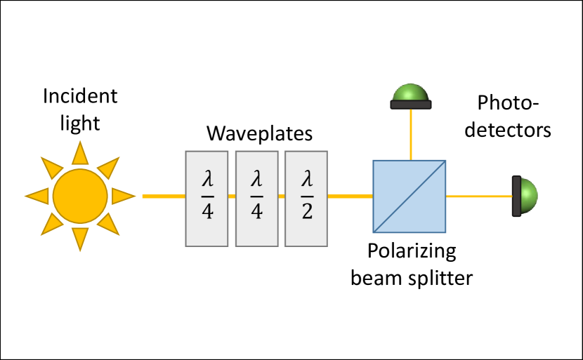
Figure 1: SU(2) gadget for measuring Stokes parameters. The polarizing beam splitter (PBS) separates the horizontal and vertical components of the light to have their intensities measured by separate photodetectors. The two quarter waveplates (“$\lambda/4$”) and one half waveplate (“$\lambda/2$”) are sufficient to enact any polarization rotation, such that the PBS can split the light into any pair of orthogonal polarization components. The original scheme by Simon and Mukunda [346] used two quarter waveplates and two half waveplates but modern schemes reduce this number [327] and the order of the waveplates is immaterial [346].

The SU(2) gadget is useful for serially measuring all of the Stokes parameters, but what if one desires to measure all four parameters simultaneously? One trick is to first divide the light into three beams and then measure three different orthogonal pairs of polarization intensities as with a single SU(2) gadget [31, 28, 30]. Alternatively, one can employ an SU(2) gadget whose waveplates rotate continuously, such that one can recover the Stokes parameters from the ensuing interferograms [156, 326]. More intricacies are required if one wants to measure the quantum polarization properties of a beam of light, such as by appropriately splitting the light into eight beams [17, 18].

Instead of waveplates, liquid crystals can also be used in creating an SU(2) gadget. Then, instead of rotating waveplates to change the polarization direction, one can adjust the voltage applied to the liquid crystals to enact the same transformation [248]. This method is a promising new tool in the polarimeter’s arsenal [358].

According to classical electrodymanics, all of the polarization components can be measured with arbitrary precision. This is in contradistinction with quantum polarization, where we will see explicitly that there exists a lower limit to the precision with which all of the Stokes parameters can be simultaneously measured.

II.3 Changes in Polarization

Polarimetry is useful because changes in polarization contain useful information about objects being measured. There are a few related methods for arranging this information, which we explore in turn.

II.3.1 Jones Matrix Calculus

The most basic question to ask is how an electric field changes when it interacts with an object. When these transformations are linear, the most general possible result is

$$\mathbf{A}^{(\mathrm{in})}\to\mathbf{A}^{(\mathrm{out})}=\mathbf{J}\mathbf{A}^{(\mathrm{in})}\qquad\iff\qquad\mathbf{E}^{(\mathrm{in})}\to\mathbf{E}^{(\mathrm{out})}=\mathbf{J}\mathbf{E}^{(\mathrm{in})},$$ (25)

where $\mathbf{J}$ is a $2\times 2$ complex matrix known as the Jones matrix. These transformations are deemed “nondepolarizing” polarization transformations because they do not change the degree of polarization of perfectly polarized states. A range of physical and linguistic arguments in favour of adopting the nomenclature “deterministic” instead of “nondepolarizing” are due to Simon [345], but we will see that this is at odds with the standard quantum definition of deterministic transformations.

When the electric field undergoes a Jones matrix transformation, the coherency matrix transforms as

$$\bm{\Psi}^{(\mathrm{in})}\to\bm{\Psi}^{(\mathrm{out})}=\mathbf{J}\bm{\Psi}^{(\mathrm{in})}\mathbf{J}^{\dagger}.$$ (26)

This equation now holds even for quasimonochromatic incident light. Then, there are some linear transformations that cannot be described by a single Jones matrix transformation. Instead, the most general linear transformation of the coherency matrix is

$$\bm{\Psi}^{(\mathrm{in})}\to\bm{\Psi}^{(\mathrm{out})}=\sum_{i}\mathbf{J}_{i}\bm{\Psi}^{(\mathrm{in})}\mathbf{J}_{i}^{\dagger},$$ (27)

where each $2\times 2$ complex matrix $\mathbf{J}_{i}$ describes a deterministic transformation. These new transformations with more than a single $\mathbf{J}_{i}$ are termed “depolarizing” or “nondeterministic” and distinctions between the two types of transformations have been investigated thoroughly [210, 345, 230, 2, 122, 36, 343, 132, 344, 93, 72, 224, 275, 74, 225, 24, 181, 94, 158, 159, 133, 114, 406].

What cannot be described by convex combinations of Jones matrix transformations are linear transformations of the form

$$\bm{\Psi}^{(\mathrm{in})}\to\bm{\Psi}^{(\mathrm{out})}=\sum_{i}\lambda_{i}\mathbf{J}_{i}\bm{\Psi}^{(\mathrm{in})}\mathbf{J}_{i}^{\dagger}$$ (28)

with negative “weights” $\lambda_{i}$. The standard assumption is that only transformations with positive weights $\lambda_{i}>0$ are physically viable [95], which is equivalent to requiring the transformations of the coherency matrix to be completely positive in the sense of Choi’s theorem [12, 13, 360, 123]. This allows us to interpret nondeterministic transformations as probabilistic mixtures of Jones matrix transformations.

Transformations governed by a single Jones matrix can result from a number of physical processes. Standard electrodynamic theory dictates that different polarizations of light have different probabilities of being reflected off of a surface and, in terms of transmission, different polarization components experience different indices of refraction, leading to the development of a relative phase between the components [193]. In turn, different physical interactions lead to different transformations of the coherency matrix. By preparing a variety of states of light with known input coherency matrices and measuring the output coherency matrices after the physical interaction, one can identify the full Jones matrix description of the interaction and thereby classify the object with which the light interacted.

II.3.2 Mueller Matrix Calculus

Linear polarization transformations are naturally described by the Stokes vector transformation

$$\mathcal{S}^{(\mathrm{in})}\to\mathcal{S}^{(\mathrm{out})}=\mathbf{M}\mathcal{S}^{(\mathrm{in})}.$$ (29)

Here, the $4\times 4$ real Mueller matrix $\mathbf{M}$ encodes all of the possible classical information that can be garnered from a linear polarization transformation. As with coherency matrices, by preparing a variety of input states of light with known Stokes parameters and measuring the output Stokes parameters after the physical interaction, one can identify the full Mueller matrix description of the interaction and thereby classify the object with which the light interacted [171]. For example, in the type of polarimetry alternatively known as transmission ellipsometry, one compares the measured $\mathbf{M}$ to various models of Mueller matrices for a medium through which the light has passed [29]. Linearity lets one assume that all sets of input Stokes parameters transform according to an identical Mueller matrix when transmitted through the same physical system, such that all $16$ components of $\mathbf{M}$ can be estimated using the same set of probe beams without any a priori knowledge of the object being measured.

Mueller matrices corresponding to Jones matrix transformations can be calculated using

$$M_{\mu\nu}=\frac{1}{2}\mathop{\mathrm{Tr}}\nolimits\left(\sigma_{\mu}\mathbf{J}\sigma_{\nu}\mathbf{J}^{\dagger}\right).$$ (30)

This compact correspondence is yet another motivation for singling out circular polarization in our basis elements. Similarly, Mueller matrices corresponding to nondeterministic polarization transformations can be calculated through

$$M_{\mu\nu}=\sum_{i}\lambda_{i}\frac{1}{2}\mathop{\mathrm{Tr}}\nolimits\left(\sigma_{\mu}\mathbf{J}_{i}\sigma_{\nu}\mathbf{J}_{i}^{\dagger}\right).$$ (31)

While it is clear that Mueller matrices can exist with $\lambda_{i}<0$, such as the matrix

$$\mathbf{M}=\begin{pmatrix}1&0&0&0\\ 0&1&0&0\\ 0&0&1&0\\ 0&0&0&-\frac{1}{3}\end{pmatrix},$$ (32)

which corresponds to a transformation of the coherency matrix with a negative weight

$$\bm{\Psi}^{(\mathrm{out})}=\frac{2}{3}\sigma_{0}\bm{\Psi}^{(\mathrm{in})}\sigma_{0}+\frac{1}{3}\sigma_{1}\bm{\Psi}^{(\mathrm{in})}\sigma_{1}+\frac{1}{3}\sigma_{2}\bm{\Psi}^{(\mathrm{in})}\sigma_{2}-\frac{1}{3}\sigma_{3}\bm{\Psi}^{(\mathrm{in})}\sigma_{3},$$ (33)

it is contended that such transformations are not physically viable. Evidence to the contrary [297] must be investigated on a case-by-case basis.

II.3.3 Deterministic Transformations in terms of Scale Factor and SL$(2,\mathds{C})$

There are four free complex components of a generic Jones matrix. However, the global phase of $\mathbf{J}$ is irrelevant in its action on the coherency matrix, as it cancels in Eq. (26), and does not show up in Mueller matrices, as it cancels in Eq. (30), so deterministic polarizations transformations are determined by seven parameters. In this and the next subsection we present a number of equivalent ways to organize these parameters, each of which comes with its own physical insights.

Removing an overall multiplicative factor from a Jones matrix can always lead to the decomposition

$$\mathbf{J}=t\pmb{J},$$ (34)

where $t\leq 1$ is an overall attenuation factor and $\pmb{J}$ belongs to the group of complex $2\times 2$ matrices with unit determinant SL$(2,\mathds{C})$, except in limiting situations in which $\det\mathbf{J}=0$. The factor $t$ does not affect the degree or direction of polarization, merely lowering $S_{0}$ by a factor of $t^{2}$ and shrinking the radius of the Poincaré sphere accordingly. One can separate measurement of the the scale factor from the other changes in polarization, by first measuring the total intensity of the transmitted beam, which transforms as

$$S_{0}\to t^{2}S_{0},$$ (35)

then separately determining the changes in orientation and length of the vector $\mathbf{S}$ normalized by the new intensity $t^{2}S_{0}$ to determine the corresponding matrix $\pmb{J}$.

After dealing with the scale factor $t$, all Jones matrices are fundamentally related to the Lorentz group. This is because transformation matrices $\pmb{J}$ maintain the quadratic form [35]

$$\mu^{2}=S_{0}^{2}-\mathbf{S}\cdot\mathbf{S},$$ (36)

as with four vectors in special relativity. Deterministic polarization transformations can thus be though of as Lorentz transformations, with some transformations corresponding to rotations of the vector $\mathbf{S}$ and others corresponding to boosts along a particular axis. To rotate the polarization vector $\mathbf{S}$ by an angle $\Theta$ about the $\mathbf{n}$-axis, we employ a Jones matrix of the form

$$\pmb{J}_{\mathrm{rot}}\left(\Theta,\mathbf{n}\right)=\exp\left(-\text{i}\Theta\mathbf{n}\cdot\bm{\sigma}/2\right).$$ (37)

Equation (37) is an example of an SU(2) rotation generated by the vector of Pauli matrices $\bm{\sigma}=\left(\sigma_{1},\sigma_{2},\sigma_{3}\right)^{\top}$.

When the electric field undergoes a rotation transformation $\mathbf{A}\to\pmb{J}_{\mathrm{rot}}\mathbf{A}$, its polarization properties correspondingly rotate in the Poincaré sphere. This is described by a Mueller matrix of the form

$$\mathbf{M}_{\mathrm{rot}}\left(\Theta,\mathbf{n}\right)=\begin{pmatrix}1&\mathbf{0}^{\top}\\ \mathbf{0}&\mathbf{R}\left(\Theta,\mathbf{n}\right)\end{pmatrix},$$ (38)

where $\mathbf{R}\left(\Theta,\mathbf{n}\right)$ is a standard $3\times 3$ rotation matrix that can be parametrized by a rotation angle $\Theta$ and axis of rotation $\mathbf{n}$, or equivalently by three Euler angles or another triad of parameters. We explicitly give one parametrization of $\mathbf{R}$ through the Rodrigues rotation formula

$$R_{ij}\left(\Theta,\mathbf{n}\right)=\delta_{ij}\cos\Theta-\sum_{k=1}^{3}\epsilon_{ijk}n_{k}\sin\Theta+n_{i}n_{j}\left(1-\cos\Theta\right),$$ (39)

where $\epsilon_{ijk}$ is the Levi-Civita tensor. Rotations leaves the $S_{0}$ component unchanged, which accords with waveplates not changing the intensity of an incident beam of light, and maintains the length of $\mathbf{S}$, as such transformations do not affect light’s degree of polarization. These properties carry through to the quantum description of polarization. We remark that these rotations are polarization rotations, in the sense that they rotate the polarization vector $\mathbf{S}$ in the Poincaré sphere and not in three-dimensional space; the effect of rotating a beam of light in three dimensions can be found in various works by Białynicki-Birula [47], Białynicki-Birula and Białynicka-Birula [48].

Similarly to the rotations expressed by Eq. (37), to boost the Stokes vector along the $\mathbf{n}$-axis by a rapidity $\eta$, we employ the Jones matrix

$$\pmb{J}_{\mathrm{boost}}\left(\eta,\mathbf{n}\right)=\exp\left(\eta\mathbf{n}\cdot\bm{\sigma}/2\right).$$ (40)

Eq. (40) differs from Eq. (37) by the crucial difference that the argument of the exponential is now real, so the Lorentz boost transformations can be thought of as rotations by an imaginary phase (or as hyperbolic rotations).

Readers versed in special relativity may be more familiar with the $4\times 4$ representation of the Lorentz group, which is directly provided by Mueller matrices. Using Eq. (30), we can immediately match the various types of transformations with the more well-known representation. For example, a boost by “rapidity” $\eta$ along the $\mathbf{e}_{3}$ axis corresponds to the Mueller matrix

$$\mathbf{M}_{\mathrm{boost}}\left(\eta,\mathbf{e}_{3}\right)=\exp\left[\eta\begin{pmatrix}0&0&0&1\\ 0&0&0&0\\ 0&0&0&0\\ 1&0&0&0\end{pmatrix}\right]=\begin{pmatrix}\cosh\eta&0&0&\sinh\eta\\ 0&1&0&0\\ 0&0&1&0\\ \sinh\eta&0&0&\cosh\eta\end{pmatrix},$$ (41)

which is exactly the transformation matrix for “boosts” between reference frames with constant relative velocity. Technically, Jones matrices correspond to the “proper” Lorentz group SO$\vphantom{a}(1,3)$, which removes the possibility of “spatial” reflections of the polarization vector $\mathbf{S}$ such as in Eq. (32). By disallowing spatial reflections, the proper Lorentz group is comprised only from rotations and boosts, each with three real parameters corresponding to the axis and strength of the transformations. This lets us arrange the seven free parameters of deterministic polarization transformations into:

• The intensity reduction factor $t$.

• The restricted Lorentz transformation $\pmb{J}$:

  • Three parameters describing the rotation $\pmb{J}_{\mathrm{rot}}$.

  • Three parameters describing the boost $\pmb{J}_{\mathrm{boost}}$.

Incidentally, the matrix polar decomposition guarantees that the Lorentz transformations can always be decomposed into a nonunique product of a single rotation and a single boost, as [249]

$$\pmb{J}=\pmb{J}_{\mathrm{rot}}\left(\Theta,\mathbf{n}_{1}\right)\pmb{J}_{\mathrm{boost}}\left(\eta,\mathbf{n}_{2}\right)=\pmb{J}_{\mathrm{boost}}\left(\eta^{\prime},\mathbf{n}_{2}^{\prime}\right)\pmb{J}_{\mathrm{rot}}\left(\Theta,\mathbf{n}_{1}\right).$$ (42)

A deterministic polarization transformation, described by a single Jones matrix, can thus always be interpreted as resulting from an intensity reduction, a rotation, and a boost applied sequentially, in any order, to an incident beam of light’s polarization degrees of freedom.

We note that the composition of two rotations is another rotation, while the same does not hold true for two boosts. Instead, the product of two boosts becomes the composition of a boost and a rotation. This extra rotation is present in many physical situations [263, 378], such as through the Thomas precession in special relativity [369] and the Wigner rotation in mathematical physics [395]. This effect has indeed been investigated for light’s polarization degrees of freedom [383, 384, 287, 286, 285], with the fascinating mathematical equivalence between indices of refraction for polarized light traveling through planar media and relative velocities of inertial frames in special relativity [383].

II.3.4 Deterministic Transformations in terms of Rotation and Diattenuation

While the rotation transformations seen above are readily enacted by waveplates and liquid crystals, it is not immediately obvious to what laboratory equipment a Lorentz boost corresponds. Fortunately, the three boost parameters and the intensity reduction factor can be alternatively arranged into four “diattenuation” parameters, which is so named because diattenuations attenuate each of the field’s polarization components by a different amount.

The simplest example of a diattenuation is when the two circular components of polarization are each diminished by a different amount:

$$\mathbf{J}_{\mathrm{diatten}}\left(q,r,\mathbf{e}_{3}\right)\begin{pmatrix}a\\ b\end{pmatrix}=\begin{pmatrix}a\sqrt{q}\\ b\sqrt{r}\end{pmatrix}.$$ (43)

This transformation can arise from, for example, light reflecting off of a surface where there is a difference in reflectivity for electric fields that are parallel versus perpendicular to the plane of reflection [193]. We can compare this transformation with Eqs. (34) and (40) to reveal the correspondences

$$q =t^{2}\text{e}^{\eta}$$ (44)

$$r =t^{2}\text{e}^{-\eta}.$$

Since attenuations only serve to decrease the intensity of light in any mode, we can use the requirements $q,r\leq 1$ to provide physical constraints on the boost and overall transmission parameters from Eqs. (34) and (40). For example, a polarizer that transmits only left-handed circularly polarized light but not its right-handed counterpart is described by the pair $\left(q,r\right)=\left(0,1\right)$; this then implies the limit of an infinite boost $\eta\to-\infty$ along the $\mathbf{e}_{3}$ axis, subject to the constraint $t=\exp\left(\eta/2\right)$.

We can also determine the Mueller matrices for arbitrary diattenuations using Eq. (30). The above example of a boost along the $\mathbf{e}_{3}$ axis, with Jones matrix given by Eq. (43), corresponds to the Mueller matrix

$$\mathbf{M}_{\mathrm{diatten}}\left(q,r,\pmb{e}_{3}\right)=\begin{pmatrix}\frac{q+r}{2}&0&0&\frac{q-r}{2}\\ 0&\sqrt{qr}&0&0\\ 0&0&\sqrt{qr}&0\\ \frac{q-r}{2}&0&0&\frac{q+r}{2}\end{pmatrix}.$$ (45)

Following a diattenuation, the total intensity $S_{0}$ decreases unless both $q$ and $r$ are equal to unity and all four Stokes parameters may decrease in magnitude. In the example of extreme attenuation corresponding to a polarizer, two components of $\mathbf{S}$ are completely nullified and the intensity of the retained component depends only on the original intensity of that component alone. The two polarizers to which our Eqs. (43) and (45) may refer are

$$\pmb{M}_{\mathrm{diatten}}\left(1,0,\mathbf{e}_{3}\right)=\begin{pmatrix}\frac{1}{2}&0&0&\frac{1}{2}\\ 0&0&0&0\\ 0&0&0&0\\ \frac{1}{2}&0&0&\frac{1}{2}\end{pmatrix}\qquad\iff\qquad I_{\mathrm{R}}+I_{\mathrm{L}}\to I_{\mathrm{R}}$$ (46)

and

$$\pmb{M}_{\mathrm{diatten}}\left(0,1,\mathbf{e}_{3}\right)=\begin{pmatrix}\frac{1}{2}&0&0&-\frac{1}{2}\\ 0&0&0&0\\ 0&0&0&0\\ -\frac{1}{2}&0&0&\frac{1}{2}\end{pmatrix}\qquad\iff\qquad I_{\mathrm{R}}+I_{\mathrm{L}}\to I_{\mathrm{L}}.$$ (47)

The two other free parameters, in addition to $q$ and $r$, in a general diattentuation are the two angular coordinates of $\mathbf{n}$ dictating which two orthogonal modes are being attenuated. A general diattenuation is physically equivalent to first rotating the polarization such that the modes to be attenuated are $\mathrm{R}$ and $\mathrm{L}$, next applying the diattenuation given by Eqs. (43) and (45), and finally rotating the light back to its original polarization orientation. Even though a general rotation depends on three parameters, these rotations here depend only on the two parameters required to enact the rotation

$$\mathbf{R}\left(\mathbf{n}\to\mathbf{e}_{3}\right)\mathbf{n}=\mathbf{e}_{3}.$$ (48)

As such, more than one rotation is sufficient to describe this situation. Using any of these rotations, which are all orthogonal in the sense that $\mathbf{R}\left(\mathbf{n}\to\mathbf{e}_{3}\right)^{\top}=\mathbf{R}\left(\mathbf{n}\to\mathbf{e}_{3}\right)^{-1}=\mathbf{R}\left(\mathbf{e}_{3}\to\mathbf{n}\right)$, we can write the most general diattenuation transformation as

$$\mathbf{M}_{\mathrm{diatten}}\left(q,r,\mathbf{n}\right) =\mathbf{M}_{\mathrm{rot}}\left(\mathbf{n}\to\mathbf{e}_{3}\right)^{-1}\mathbf{M}_{\mathrm{diatten}}\left(q,r,\mathbf{e}_{3}\right)\mathbf{M}_{\mathrm{rot}}\left(\mathbf{n}\to\mathbf{e}_{3}\right)$$ (49)

$$=\begin{pmatrix}1&\mathbf{0}^{\top}\\ \mathbf{0}&\mathbf{R}\left(\mathbf{e}_{3}\to\mathbf{n}\right)\end{pmatrix}\begin{pmatrix}\frac{q+r}{2}&0&0&\frac{q-r}{2}\\ 0&\sqrt{qr}&0&0\\ 0&0&\sqrt{qr}&0\\ \frac{q-r}{2}&0&0&\frac{q+r}{2}\end{pmatrix}\begin{pmatrix}1&\mathbf{0}^{\top}\\ \mathbf{0}&\mathbf{R}\left(\mathbf{n}\to\mathbf{e}_{3}\right)\end{pmatrix}.$$

Combining diattenuations with the matrix polar decomposition, any deterministic polarization transformation given by a single Jones matrix can be composed from a single rotation and a single diattenuation transformation, in either order [249]. As the set of rotations forms a group under multiplication and inversion, we conclude that arbitrary deterministic polarization transformations can be obtained from waveplates and a single diattenuating element.

II.3.5 Nondeterministic Transformations

Deterministic transformations account for seven of the $16$ degrees of freedom of a general polarization transformation contained by the Mueller matrices of Eq. (29). The remaining nine parameters must arise from transformations requiring more than a single Jones matrix, such as through the convex combination in Eq. (27), which is what gives rise to the “nondeterministic” nomenclature. Such transformations are also denoted as depolarizing because they almost always depolarize incident light that is perfectly polarized light (unless they simply do not effect any transformation on the latter).

Nondeterministic polarization transformations are usually ascribed to the inability to experimentally discriminate between physical processes that each enact a different deterministic polarization transformation, as opposed to arising from fundamentally indeterminate laws of nature [135]. For example, when a detector absorbs photons with a range of frequencies that are present in a quasimonochromatic beam of light and each frequency experiences a different polarization rotation after travelling through a birefringent crystal, the resultant polarization state must be taken to be the convex combination of the polarization states of the various frequency components, each with their individual polarization rotations [247, 245, 108, 81]. Similarly, light whose polarization is rotated more quickly than can be resolved by a detector will have its degree of polarization reduced accordingly [50]. Finally, light scattering off of optically active media has its polarization change depending on the direction of scattering [81], so a detector receiving light from a nonzero range of solid angles leads to convex combinations of the deterministic processes ascribed to each scattering angle. These examples are well summarized by the assertion that that all depolarization processes can, in principle, be reversed but cannot be reversed in practice [247].

The simplest example of a nondeterministic polarization transformation is that of an ideal depolarizer, whose Mueller matrix reads

$$\mathbf{M}_{\mathrm{depol}}=\begin{pmatrix}1&0&0&0\\ 0&0&0&0\\ 0&0&0&0\\ 0&0&0&0\end{pmatrix}.$$ (50)

An ideal depolarizer maintains $S_{0}$, leaving the total intensity and total energy of the light unchanged, while enacting $p\to 0$, regardless of the input state. Equivalently, an ideal depolarizer transforms the perfectly polarized component of the beam represented in Eqs. (23) and (24) into a completely unpolarized component. The polarization scrambling methods mentioned are made to simulate ideal depolarizers [247], with work continuing to be done in this field of depolarizer design [407, 125, 335, 266, 227, 267].

Nondeterministic polarization transformations do not affect the total intensity $S_{0}$, only altering the polarization vector $\mathbf{S}$. The nine remaining parameters of general nondeterministic (“depolarizing”) Mueller matrices take the form of a $3\times 3$ symmetric real matrix $\mathbf{m}$ and a real vector $\mathbf{p}$ with magnitude less than or equal to unity [249]:

$$\mathbf{M}_{\mathrm{depol}}=\begin{pmatrix}1&\mathbf{0}^{\top}\\ \mathbf{p}&\mathbf{m}\end{pmatrix}.$$ (51)

The assumption that only positive weights feature in Eqs. (28) and (31) restricts the matrix $\mathbf{m}$ to being positive [135], which precludes transformations of the form of Eq. (32). Under some physical assumptions, such matrices can always be decomposed into the product of a single diattenuation, a single rotation, and a single depolarizing transformation with $\mathbf{p}=0$, through [135]

$$\mathbf{M}_{\mathrm{depol}}=\mathbf{M}_{\mathrm{rot}}\left(\Theta,\mathbf{n}\right)\mathbf{M}_{\mathrm{diatten}}\left(q,r,\mathbf{n^{\prime}}\right)\begin{pmatrix}1&\mathbf{0}^{\top}\\ \mathbf{0}&\mathbf{m^{\prime}}\end{pmatrix}.$$ (52)

How can we achieve an ideal depolarizer using this formalism? We note that, due to Eq. (31), nondeterministic Mueller matrices come from probabilistic mixtures of deterministic Mueller matrices

$$\bm{\Psi}\to\sum_{i}\lambda_{i}\mathbf{J}_{i}\bm{\Psi}\mathbf{J}_{i}^{\dagger}\qquad\Rightarrow\qquad\mathbf{M}=\sum_{i}\lambda_{i}\mathbf{M}_{i}.$$ (53)

If each of the deterministic transformations in the combination correspond to a rotation by angle $\Theta_{i}$ about axis $\mathbf{n}_{i}$, we achieve a depolarizing transformation with $\mathbf{p}=0$ and $\mathbf{m}=\sum_{i}\lambda_{i}\mathbf{R}\left(\Theta_{i},\mathbf{n}_{i}\right)$. A sufficient number of rotations in a sufficient number of directions leads to $\mathbf{m}=\mathbf{0}\mathbf{0}^{\top}$. We further note that an arbitrary symmetric matrix $\mathbf{m}$ can be obtained from a convex combination of sufficiently many rotation matrices with appropriate weights, provided that those weights are allowed to be negative [144]. Otherwise, only positive matrices $\mathbf{m}$ can be generated.

We collect two few key facts before proceeding. First, any polarization transformation can be realized by the sequential application of a rotation, a diattenuation, and a depolarization, in any order [249, 134]. Next, all such transformations can be realized via convex combinations of four or fewer deterministic transformations [95]. We thereby possess a complete description of all polarization transformations from a classical perspective.

II.3.6 Physical Constraints on Polarization Changes

Many works have investigated physical constraints on the viability of various Jones and Mueller matrices [122, 343, 132, 93, 275, 181, 133, 406, 95, 249, 182, 37, 140, 293, 342, 412, 134]. We will not review all of them here, instead focusing on a few constraints that become relevant in the quantum theory of polarimetry.

Foremost, polarization changes are only considered to be physically viable if they are composed of probabilistic mixtures of pure Jones transformations, equivalent to Eqs. (28) and (31) restricted to $\lambda_{i}>0$. This assertion can be traced to Cloude [95], which we will quote directly due to the challenge of obtaining this reference: “What are the weighting coefficients [$\lambda_{i}$] and how are they determined?” They proceed to answer this question “by considering a new formulation of the scattering problem” based on rearranging the elements of a rescaled Jones matrix $\pmb{J}$ into a $4\times 1$ vector $\mathcal{K}$. Then, a general Mueller matrix can be formed by taking linear combinations of the outer products $\mathbf{T}=\sum_{i}\lambda_{i}\mathcal{K}_{i}\mathcal{K}_{i}^{\dagger}$, eventually giving rise to Eq. (31) with the eigenvalues of $\mathbf{T}$, $\lambda_{i}$, acting as the weights up to unitary transformations (“plane rotations in a 6 dimensional real target space”). This leads to the assertion that, because $\mathbf{T}$ “is a complex correlation matrix [with] a much clearer physical interpretation than the Mueller matrix,” it follows that “the eigenvalues are positive real and each eigenvector corresponds . . . to a single scattering matrix.” Physically, no reason is provided to prohibit a single Mueller matrix of the form of Eq. (32) arising on its own in nature other than the, perhaps circular, perhaps physically reasonable, assertion that all Mueller matrices arise from probabilistic mixtures of deterministic transformations associated with single Jones matrices.

A flurry of attention revisited this problem motivated by quantum theory [12, 13, 360, 342, 123], which we have conjectured to truly underlie the necessity of positive weights in Eqs. (28) and (31) [144]. It was first noted that the transformations responsible for transforming coherency matrices look like completely positive quantum channels, where the Jones matrices of Eq. (27) can be thought of as Kraus operators [12, 13, 360, 123]. This hints at the well-known connection with the quantum theory of polarization, viz., that single photons have density matrices described by their coherency matrices $\bm{\Psi}$; the transformations of classical polarization states are akin to transformations of single-photon polarization states. Then, all physically viable transformations that take single-photon polarization states to single-photon polarization states must be completely positive, immediately restricting the weights in Eqs. (28) and (31) to be positive. We learn that, if all light were to be described by the behaviours of single photons (which precludes studies of attenuation), quantum theory would enforce the positivity assertion of classical polarization transformations. Then, inspired by a phenomenon known as “nonquantum entanglement,” Simon et al. [342] showed that the only way for an extended version of Eq. (15) to hold is through the positivity assertion of classical polarization transformations. In the extended version, the Stokes parameters are extended to two-point correlation functions, wherein the electric fields are taken to be at different points in the $x$-$y$ plane [cf. Eq. (13)]:

$$S_{\mu}\left(x,y;x^{\prime},y^{\prime}\right)=\frac{1}{2}\langle\mathbf{E}\left(x^{\prime},y^{\prime},z;t\right)^{\dagger}\sigma_{\mu}\mathbf{E}\left(x,y,z;t\right)\rangle.$$ (54)

In order to act linearly on these extended Stokes parameters, Mueller matrices must be made from positive-weight combinations of deterministic elements. Of course, this is asking more of Mueller matrices than the standard definition in Eq. (29), so it remains to be proven whether the necessity of positive weights in Eqs. (28) and (31) follows from any deeper physical condition.

The most natural constraint on Mueller and Jones matrices is that they take physically viable polarization states to physically viable polarization states. This means that all linear polarization transformations must ensure their output states satisfy the constraint of Eq. (15) regardless of the input state. All pure Jones matrices automatically satisfy this constraint, as do convex combinations thereof, so we learn that the 16 parameters of a polarization transformation are not independently free, instead satisfying

$$\mathrm{Tr}\left(\mathbf{M}\mathbf{M}^{\top}\right)\leq 4M_{0,0}^{2}.$$ (55)

Finally, we mention the transmittance and reverse transmittance conditions for Mueller matrices [133]. Under the assumption that a single deterministic transformation does not increase the intensity of an incident beam, it can be verified that any Mueller matrix arising from a single deterministic transformation satisfies

$$M_{0,0}+\sqrt{M_{0,1}^{2}+M_{0,2}^{2}+M_{0,3}^{2}}=M_{0,0}+\sqrt{M_{1,0}^{2}+M_{2,0}^{2}+M_{3,0}^{2}}\leq 1\,\,\iff\,\,\mathrm{Tr}\left(\mathbf{M}\mathbf{M}^{\top}\right)=4M_{0,0}^{2}.$$ (56)

Then, any Mueller matrix arising from a convex combination of deterministic elements must satisfy

$$M_{0,0}+\sqrt{M_{0,1}^{2}+M_{0,2}^{2}+M_{0,3}^{2}} \leq 1\qquad\mathrm{and}\qquad M_{0,0}+\sqrt{M_{1,0}^{2}+M_{2,0}^{2}+M_{3,0}^{2}} \leq 1$$ (57)

$$\qquad\iff\qquad\lambda_{i}>0\mathrm{\,in\,Eqs.\,\eqref{eq:coherency multiple Jones with weights}\,and\,\eqref{eq:Mueller from Jones with weights}}.$$

These conditions preclude the possibility of transformations such as lossless polarizers, which would be able to convert all input light of a given polarization component into light with the opposite component regardless of input beam, such as

$$\mathbf{M}_{\mathrm{lossless\,polarizer}}=\begin{pmatrix}1&0&0&0\\ 0&0&0&0\\ 0&0&0&0\\ 1&0&0&0\end{pmatrix}.$$ (58)

It turns out that we can concoct polarization transformations that satisfy all of the requisite conditions, even that of positive weights, while breaking the transmittance conditions. For example, we can consider the pair of pure Jones matrices

$$\mathbf{J}_{1}=\begin{pmatrix}1&0\\ 0&0\end{pmatrix}\qquad\mathrm{and}\qquad\mathbf{J}_{2}=\begin{pmatrix}0&1\\ 0&0\end{pmatrix},$$ (59)

which directly lead to the Mueller matrix of Eq. (58) when added with $\lambda_{1}=\lambda_{2}=1$ as in Eq. (27) (similarly, if we employ $\mathbf{J}_{2}^{\top}$ instead of $\mathbf{J}_{2}$, we find $\mathbf{M}_{\mathrm{lossless\,polarizer}}^{\top}$, which disobeys the forward instead of the reverse transmittance condition). On the contrary, if we consider adding them with $\lambda_{1}=\lambda_{2}=1/2$ as in Eq. (28), we find the resulting Mueller matrix to be $\mathbf{M}=\mathbf{M}_{\mathrm{lossless\,polarizer}}/2$, which indeed satisfies the reverse transmittance condition. How should we rectify this situation? Requiring the coefficients $\lambda_{i}$ to sum to unity would suffice, because the transmittance conditions assume we cannot rescale these Jones matrices by a factor greater than unity. In contradistinction, the unital nature of quantum channels only requires Kraus operators to satisfy $\mathbf{J}_{1}^{\dagger}\mathbf{J}_{1}+\mathbf{J}_{2}^{\dagger}\mathbf{J}_{2}=\mathds{1}$, which is indeed satisfied here with $\lambda_{1}=\lambda_{2}=1$, so there seems to exist a quantum channel that would act like a lossless polarizer on a single photon. Further inspection reveals that $\mathbf{J}_{1}$ ensures that all right-handed circularly polarized light retains its polarization and $\mathbf{J}_{2}$ converts all left-handed circularly polarized light to its right-handed counterpart. This can only be achieved in a “linear” manner by a device that measures the total incident intensity, then prepares a right-handed circularly polarized state with that same intensity to be output: a highly nonlinear device poising as a linear one. Because this must hold regardless of the input Stokes parameters, it must be capable of measuring and generating output states of light with arbitrarily large intensities. These considerations prohibit such a device from being physically viable and reinforce the transmittance conditions; we will return to this consideration when discussing quantum polarization transformations.

III Quantum Polarization

Maxwell’s equations equally apply to quantized light fields. In the quantum theory, the field amplitudes $a$ and $b$ from Eq. (1) get promoted to bosonic operators $\hat{a}$ and $\hat{b}$ that annihilate right- and left-handed circularly polarized photons:

$$\hat{\mathbf{E}}=\mathcal{E}_{0}\left(\hat{a}\mathbf{e}_{a}+\hat{b}\mathbf{e}_{b}\right)\text{e}^{\text{i}\left(kz-\omega t\right)}.$$ (60)

These operators satisfy the standard bosonic commutation relations

$$\left[\hat{a},\hat{a}^{\dagger}\vphantom{a}\right]=\left[\hat{b},\hat{b}^{\dagger}\vphantom{a}\right]=1\qquad\mathrm{and}\qquad\left[\hat{a},\hat{b}^{\dagger}\vphantom{a}\right]=\left[\hat{b},\hat{a}^{\dagger}\vphantom{a}\right]=0$$ (61)

and can be used to create states with definite photon numbers in a single spatial mode from the two-mode vacuum $\lvert\mathrm{vac}\rangle$ via

$$\lvert m,n\rangle\equiv\lvert m\rangle_{\mathrm{R}}\otimes\lvert n\rangle_{\mathrm{L}}=\frac{\hat{a}^{\dagger}\vphantom{a}{}^{m}\hat{b}^{\dagger}\vphantom{a}{}^{n}}{\sqrt{m!n!}}\lvert\mathrm{vac}\rangle.$$ (62)

The intensity of the field is given by the average number of excitations $\langle\hat{a}^{\dagger}\vphantom{a}\hat{a}^{\dagger}\vphantom{a}+\hat{b}^{\dagger}\vphantom{a}\hat{b}\rangle$ and similarly for the intensities within each polarization component.

Following the above quantization rule, we can define the Stokes operators as

$$\hat{S}_{0} =\frac{\hat{n}_{\mathrm{H}}+\hat{n}_{\mathrm{V}}}{2}=\frac{\hat{n}_{\mathrm{D}}+\hat{n}_{\mathrm{A}}}{2}=\frac{\hat{n}_{\mathrm{R}}+\hat{n}_{\mathrm{L}}}{2}=\frac{\hat{a}^{\dagger}\vphantom{a}\hat{a}+\hat{b}^{\dagger}\vphantom{a}\hat{b}}{2},$$ (63)

$$\hat{S}_{1} =\frac{\hat{n}_{\mathrm{H}}-\hat{n}_{\mathrm{V}}}{2}=\frac{\hat{a}^{\dagger}\vphantom{a}\hat{b}+\hat{b}^{\dagger}\vphantom{a}\hat{a}}{2},$$

$$\hat{S}_{2} =\frac{\hat{n}_{\mathrm{D}}-\hat{n}_{\mathrm{A}}}{2}=-\text{i}\frac{\hat{a}^{\dagger}\vphantom{a}\hat{b}-\hat{b}^{\dagger}\vphantom{a}\hat{a}}{2},$$

$$\hat{S}_{3} =\frac{\hat{n}_{\mathrm{R}}-\hat{n}_{\mathrm{L}}}{2}=\frac{\hat{a}^{\dagger}\vphantom{a}\hat{a}-\hat{b}^{\dagger}\vphantom{a}\hat{b}}{2},$$

or succinctly through [cf. Eq. (13)]

$$\hat{S}_{\mu}=\frac{1}{2}\begin{pmatrix}\hat{a}^{\dagger}\vphantom{a}&\hat{b}^{\dagger}\vphantom{a}\end{pmatrix}\sigma_{\mu}\begin{pmatrix}\hat{a}\\ \hat{b}\end{pmatrix},$$ (64)

with the quantum-to-classical correspondence

$$S_{\mu}=\langle\hat{S}_{\mu}\rangle.$$ (65)

The factor of $2$ that we have been carrying through these definitions allows us to realize the Stokes operators as obeying the commutation relations of angular momentum,

$$\left[\hat{S}_{i},\hat{S}_{j}\right]=\sum_{k=1}^{3}\epsilon_{ijk}\hat{S}_{k}\qquad\mathrm{and}\qquad\left[\hat{S}_{0},\hat{S}_{i}\right]=0,$$ (66)

and we see that the Schwinger mapping [83, 295] governs the translation between two-mode states and angular momentum eigenstates.

Classically, all of the Stokes parameters can be measured with arbitrary precision. However, since they arise as expectation values of noncommuting operators, the same cannot be said at a fundamental level; instead, there is a lower limit to the joint precision with which a pair of Stokes parameters can be measured. Methods of optimizing tradeoffs such as

$$4\mathop{\mathrm{Var}}\nolimits\hat{S}_{1}\mathop{\mathrm{Var}}\nolimits\hat{S}_{2}\geq\left|\langle\hat{S}_{3}\rangle\right|^{2}$$ (67)

and

$$\mathop{\mathrm{Var}}\nolimits\hat{S}_{1}+\mathop{\mathrm{Var}}\nolimits\hat{S}_{2}+\mathop{\mathrm{Var}}\nolimits\hat{S}_{3}\geq\langle\hat{S}_{0}\rangle,$$ (68)

where we denote operator variances by $\mathop{\mathrm{Var}}\nolimits X=\langle X^{2}\rangle-\langle X\rangle^{2}$, have led to the fruitful discovery and implementation of “polarization squeezing,” which may ultimately have applications in quantum-enhanced polarimetry and other communication tasks [397, 86, 211, 177, 9, 396, 208, 20, 69, 218, 19, 165, 352, 221, 64, 1, 328, 174, 202, 23, 339, 391, 157, 175, 222, 303, 258, 337, 268, 84, 233, 278, 312, 99, 111, 191, 336, 128, 186, 260, 279, 173, 306, 259, 38, 163, 308, 91, 217, 43, 282, 85, 307, 292, 386, 392, 167, 385, 52, 33]. Polarization squeezing is significantly reviewed in Refs [259], with briefer reviews in, e.g., Refs. [372, 85, 147].

From the theory of angular momentum, we immediately find that

$$\hat{\mathbf{S}}^{2}\equiv\hat{S}_{1}^{2}+\hat{S}_{2}^{2}+\hat{S}_{3}^{2}=\hat{S}_{0}\left(\hat{S}_{0}+1\right)\geq\hat{S}_{0}^{2}.$$ (69)

This does not imply that quantum states may disobey criterion of Eq. (15), which remains true in the guise of

$$\langle\hat{S}_{1}\rangle^{2}+\langle\hat{S}_{2}\rangle^{2}+\langle\hat{S}_{3}\rangle^{2}\leq\langle\hat{S}_{0}\rangle^{2};$$ (70)

these together enforce the variance inequality in Eq. (68). Interestingly, the ultimate quantum limit with which the Stokes parameters for classical light may be simultaneously estimated obeys stricter conditions than Eq. (68):

$$\mathop{\mathrm{Var}}\nolimits\hat{S}_{1}+\mathop{\mathrm{Var}}\nolimits\hat{S}_{2}+\mathop{\mathrm{Var}}\nolimits\hat{S}_{3}\geq\frac{5}{2}\langle\hat{S}_{0}\rangle$$ (71)

when the value of $S_{0}$ is unknown [209, 273, 197] and

$$\mathop{\mathrm{Var}}\nolimits\hat{S}_{1}+\mathop{\mathrm{Var}}\nolimits\hat{S}_{2}+\mathop{\mathrm{Var}}\nolimits\hat{S}_{3}\geq 2\langle\hat{S}_{0}\rangle$$ (72)

when the value of $S_{0}$ is known a priori [197].

The four Stokes parameters can be simultaneously measured by mixing the input light with six other vacuum modes input to an interferometer and computing sum or difference currents among four particular pairs of output modes [17, 18]. Each sum or difference photocurrent yields one half of one of the Stokes parameters, even in the quantum regime, but the variances of these photocurrents are not proportional to the variances of the Stokes parameters; instead, the former are all offset from the latter by an amount proportional to the total intensity of the field and are thus never nonzero. Similar schemes can be created using interferometers with two [250, 310] or four [250, 313] input ports in their vacuum states. Mathematical postprocessing of such a measurement can be used to verify the presence of polarization squeezing and the potential saturation of inequalities such as Eq. (68).

It is instructive to investigate the properties of single-photon polarization states, spanned by $\lvert 1,0\rangle$ and $\lvert 0,1\rangle$, as these directly encompass classical polarization phenomena, which are governed by the $2\times 2$-density-matrix-like object $\bm{\Psi}$. The most general density matrix for such a state is given in this basis by

$$\hat{\rho}_{\mathrm{single\,photon}}=\begin{pmatrix}\rho_{0,0}&\rho_{1,0}^{*}\\ \rho_{1,0}&1-\rho_{0,0}\end{pmatrix},$$ (73)

subject to the constraints of positivity. The Stokes parameters are readily calculable using Pauli matrices, yielding

$$\mathcal{S}=\begin{pmatrix}\frac{1}{2}\\ \mathop{\mathrm{Re}}\nolimits\rho_{1,0}\\ \mathop{\mathrm{Im}}\nolimits\rho_{1,0}\\ \rho_{0,0}-\frac{1}{2}\end{pmatrix}.$$ (74)

The density matrix can be decomposed into density matrices corresponding to pure and maximally mixed states, via

$$\hat{\rho}_{\mathrm{single\,photon}}=\sum_{\mu=0}^{3}S_{\mu}\sigma_{\mu}=p\frac{\mathds{1}+\frac{\mathbf{S}}{\left|\mathbf{S}\right|}\cdot\bm{\sigma}}{2}+\left(1-p\right)\frac{\mathds{1}}{2},$$ (75)

where the degree of polarization is, as usual, $p=\left|\mathbf{S}\right|/S_{0}$. Pure single photons have degree of polarization $p=1$ and maximally mixed single photons have $p=0$, which can alternatively be expressed via the purity parameter $\mathop{\mathrm{Tr}}\nolimits\left(\hat{\rho}^{2}\right)$ through

$$p=\frac{\left|\mathbf{S}\right|}{S_{0}}=\sqrt{\frac{\mathop{\mathrm{Tr}}\nolimits\left(\bm{\Psi}^{2}\right)}{2S_{0}^{2}}-1}=\sqrt{2\mathop{\mathrm{Tr}}\nolimits\left(\hat{\rho}^{2}\right)-1}.$$ (76)

The density matrix for single photons thus completely reproduces the classical coherency matrix for describing polarization states. We next explore properties of quantum states with more than a single photon.

III.1 Characterizing Polarization

The Stokes operators presented in Eq. (63) conserve photon number, as each creation operator is paired with an annihilation operator. This is one way to see why they commute with the total-photon-number operator $\hat{N}=2\hat{S}_{0}$ and ensures that the polarization properties of a beam of light can be broken into the polarization properties of each photon-number subspace, where the latter are sometimes called Fock layers [110, 292]. We next explore the polarization properties of pure states with a fixed number of photons $N$, equivalent to states with spin $N/2$, whose most general form is given by

$$\lvert\psi^{(N)}\rangle=\sum_{m=0}^{N}\psi_{m}\lvert m,N-m\rangle,\qquad\sum_{m=0}^{N}\left|\psi_{m}\right|^{2}=1.$$ (77)

Geometrically, it is easy to visualize pure single-photon states on the surface of the Poincaré (or Bloch) sphere, as they can be parametrized by two angular coordinates $\Omega=\left(\Theta,\Phi\right)$:

$$\lvert\Omega^{(1)}\rangle=\cos\frac{\Theta}{2}\lvert 1,0\rangle+\text{e}^{\text{i}\Phi}\sin\frac{\Theta}{2}\lvert 0,1\rangle.$$ (78)

We can alternatively write these states as resulting from the action of a single creation operator, parametrized by $\Omega$, acting on the two-mode vacuum, through

$$\lvert\Omega^{(1)}\rangle=\hat{a}_{\Omega}^{\dagger}\lvert\mathrm{vac}\rangle,\qquad\hat{a}_{\Omega}^{\dagger}=\cos\frac{\Theta}{2}\hat{a}^{\dagger}\vphantom{a}+\text{e}^{\text{i}\Phi}\sin\frac{\Theta}{2}\hat{b}^{\dagger}\vphantom{a}.$$ (79)

However, we cannot visualize an $N$-photon state as a series of $N$ Poincaré spheres, as the photons are, in general, mutually correlated. This challenge is addressed by the Majorana representation [261, 44].

The Majorana representation begins by realizing the one-to-one correspondence between the amplitudes $\left\{\psi_{m}\right\}$ and the set of $N$ angular coordinates $\left\{\Omega_{k}\right\}$, through

$$\lvert\psi^{(N)}\rangle=\frac{1}{\sqrt{\mathcal{N}}}\prod_{k=1}^{N}\hat{a}_{\Omega_{k}}^{\dagger}\lvert\mathrm{vac}\rangle,$$ (80)

where the normalization constant $\mathcal{N}$ depends on the coordinates and does not affect the geometry of the state. This correspondence allows us to represent any $N$-photon pure state by a constellation of $N$ points on the surface of a sphere, where each point is sometimes referred to as a star in the Majorana constellation. Notably, the entire constellation rotates rigidly under a polarization rotation, lending geometric intuition to multiphoton polarization states. The usefulness of the Majorana representation has been realized in topics from metrology [89, 61, 149, 270, 144, 152, 90] to Bose-Einstein condensates [236, 102] to non-Hermitian physics [39] and beyond [168, 169, 55, 53, 139, 220, 262, 269, 232, 76, 381, 403, 238, 80, 109]. We exemplify some Majorana constellations in Fig. 2 and note that states whose Majorana constellations are randomly distributed have intriguing properties that are only now being elucidated [143].

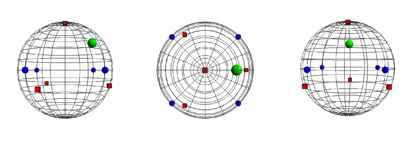
Figure 2: Three views of three different Majorana constellations for four-photon states. The large green ball corresponds to the fourfold degenerate constellation of an SU(2)-coherent state with $\Omega_{1}=\Omega_{2}=\Omega_{3}=\Omega_{4}$, the smaller blue balls correspond to a NOON state with Majorana stars equally spread about the equator, and the red cubes correspond to a state whose Majorana constellation is a regular tetrahedron.

The Majorana constellation, as it stands, pertains to pure $N$-photon states. What can we retain when considering more general quantum states? For mixed states with a fixed number of photons, representations have been derived that retain some of the geometrical properties of the standard constellation by either decomposing the density matrix into its eigenbasis [277] or into the spherical tensor basis [331] and finding a constellation for each element in said basis. For pure states with indeterminate numbers of photons, one can consider a Majorana representation within each photon-number subspace, where one must also keep track of the relative weights and relative phases between each subspace (ignoring the relative phases, one can consider a set of Majorana constellations for a convex combination of pure states that each have a different number of photons) [55]. Regrettably, a unified geometrical picture for arbitrary quantum states à la Majorana is still lacking.

III.1.1 Polarized States

We are now in a position to ascertain which quantum mechanical states underlie their classical counterparts with degree of polarization $p=1$ [148], expanding upon earlier work by Mehta and Sharma [276], Prakash and Singh [305], Singh and Prakash [347], Luis [256]. These quantum states have significant complementarity properties [296]. We note in passing that other degrees of polarization have been proposed in light of the quantum nature of polarization [19, 17, 214, 252, 253, 254, 256, 324, 255, 56, 126, 127, 184, 226, 54, 323], each with their own merits and motivations, but continue our investigation along the lines of the canonical degree of polarization because the proposed new degrees are mutually inconsistent in their orderings of partially polarized states [127].

The easiest example of a perfectly polarized quantum state is that of a pure single photon. This is readily generalized to pure states with exactly $N$ photons, where the resulting state is completely polarized if and only if all $N$ of the constituent photons have the same direction of polarization. In terms of the Majorana constellation, this requires all $N$ of the angular coordinates to degenerate to a single point on the surface of the sphere as in Fig. 2, with the angular coordinates of that point dictating the state’s polarization direction. These states are the well-known SU(2)-coherent, or spin-coherent, states [25]

$$\lvert\Omega^{(N)}\rangle=\frac{\hat{a}_{\Omega}^{\dagger}\vphantom{a}{}^{N}}{\sqrt{N!}}\lvert\mathrm{vac}\rangle=\sum_{m=0}^{N}\psi_{m}^{\Omega;N}\lvert m,N-m\rangle,$$ (81)

where

$$\psi_{m}^{\Omega;N}=\sqrt{\binom{N}{m}}\cos^{m}\frac{\Theta}{2}\sin^{N-m}\frac{\Theta}{2}\text{e}^{\text{i}\Phi(N-m)}.$$ (82)

SU(2)-coherent states are eigenstates of an angular momentum operator projected in the direction $\mathbf{n}_{\Omega}=\left(\sin\Theta\cos\Phi,\sin\Theta\sin\Phi,\cos\Theta\right)^{\top}$ with eigenvalue $S_{0}=N/2$:

$$\left(\hat{\mathbf{S}}\cdot\mathbf{n}_{\Omega}\right)\lvert\Omega^{(N)}\rangle=\frac{N}{2}\lvert\Omega^{(N)}\rangle$$ (83)

and have many other useful properties [300, 124]. The Stokes parameters for SU(2)-coherent states are exactly those of perfectly polarized light with intensity equal to that of $N$ photons

$$\mathcal{S}=\frac{N}{2}\begin{pmatrix}1\\ \mathbf{n}_{\Omega}\end{pmatrix}$$ (84)

and SU(2)-coherent states can be considered as spin states with maximal spin projection. Notably, these perfectly polarized states behave sensibly when undergoing polarization rotations, with the direction of polarization rotating as expected for classical beams of light.

The only states, pure or mixed, with exactly $N$ photons that are perfectly polarized are the SU(2)-coherent states of Eq. (81). The rest of the quantum states with $p=1$ must therefore have indeterminate photon number (i.e., not be eigenstates of $\hat{S}_{0}$).

One simple extension of SU(2)-coherent states is to convex combinations of SU(2)-coherent states, each with the same angular coordinates. One can prove that such states, given by

$$\hat{\rho}=\sum_{N=0}^{\infty}\rho_{N}\lvert\Omega^{(N)}\rangle\langle\Omega^{(N)}\rvert,\quad\sum_{N=0}^{\infty}\rho_{N}=1,\quad\rho_{N}\geq 0,$$ (85)

are all perfectly polarized in direction $\Omega$, with intensity equal to the average photon number (in the appropriate units) $\hat{S}_{0}\propto\sum_{N=0}^{\infty}\rho_{N}N$ [276]. Even though there is a probabilistic mixture present, all of the states in the mixture have the same direction of polarization, so they conspire to yield a state that is completely polarized overall. Equation (85) is markedly different from the case of single photons: for single photons, purity and degree of polarization are the same quantity, as seen in Eq. (76); when more than one photon number is involved, mixed states can still have degree of polarization $p=1$.

Returning momentarily from mixed states back to pure states, superpositions of SU(2)-coherent states in different photon-number subspaces whose directions of polarization are all collinear are also perfectly polarized. In fact, these are the only possible pure states with degree of polarization $p=1$ [148]:

$$\lvert\Psi\rangle=\sum_{N=0}^{\infty}\text{e}^{\text{i}\varphi_{N}}\sqrt{\rho_{N}}\lvert\Omega^{(N)}\rangle,\quad\sum_{N=0}^{\infty}\rho_{N}=1,\quad\rho_{N}\geq 0,\quad\varphi_{N}\in\mathds{R}.$$ (86)

This simply means that classical polarization properties may be underlain by quantum superpositions about which the former are ignorant, especially because even the Stokes operators themselves do not distinguish between the pure superpositions of Eq. (86) and the mixed states of Eq. (85) in any of their correlation functions. In that sense, another form of correlation gadget is required to be sensitive to these relative phases between Fock layers, as outlined in the conclusions of [151], such as by using weak-field homodyne detection [110].

The pure states we are now discussing encompass canonical coherent states, which are generally agreed to be the most classical states according to quantum optics[264]:

$$\lvert\alpha\rangle\propto\exp(\alpha\hat{a}^{\dagger}\vphantom{a})\lvert\mathrm{vac}\rangle.$$ (87)

These states obey the restrictions of Eqs. (71) and (72) in terms of their simultaneously measurable properties. From the perspective of polarization, these states take the form [26]

$$\lvert\alpha_{\Omega}\rangle\propto\exp(\alpha\hat{a}_{\Omega}^{\dagger})\lvert\mathrm{vac}\rangle=\sum_{N=0}^{\infty}\frac{\alpha^{N}}{N!}\hat{a}_{\Omega}^{\dagger}\vphantom{a}{}^{N}\lvert\mathrm{vac}\rangle=\sum_{N=0}^{\infty}\frac{\alpha^{N}}{\sqrt{N!}}\lvert\Omega^{(N)}\rangle.$$ (88)

These are the states sometimes thought to underlie classical polarization phenomena, as they can be described solely using the Stokes vector [cf. Eqs. (16) and (83)]

$$\mathcal{S}=\frac{\left|\alpha\right|^{2}}{2}\begin{pmatrix}1\\ \mathbf{n}_{\Omega}\end{pmatrix}$$ (89)

with no other free parameters (i.e., no additional “quantum” degrees of freedom present beyond the classical description), but we will see later that even this thinking has its pitfalls when we begin to consider partially polarized states.

We are now in the position to write the most general perfectly polarized quantum state:

$$\hat{\rho}=\sum_{M,N=0}^{\infty}\sigma_{M,N}\lvert\Omega^{(M)}\rangle\langle\Omega^{(N)}\rvert,\quad\mathop{\mathrm{Tr}}\nolimits\pmb{\sigma}=1,$$ (90)

for any positive-semidefinite matrix $\pmb{\sigma}$. These states can be thought of as probabilistic mixtures of pure states of the form of Eq. (86), which can also be realized using a single element from a pair of orthogonal creation operators via:

$$\hat{\rho}=\sum_{i=0}^{\infty}F_{i}\left(\hat{a}_{\Omega}^{\dagger}\right)\lvert\mathrm{vac}\rangle\langle\mathrm{vac}\rvert F_{i}^{*}\left(\hat{a}_{\Omega}\right),$$ (91)

where the functions $F_{i}(z)=\sum_{N}f_{N}^{(i)}z^{N}$ need only be normalized by a common factor. Moreover, these states arise exclusively from polarization rotations of states that have all of their excitations in a single mode, using the polarization rotation operators $\hat{R}$ that we will discuss in Section III.2.1:

$$\hat{\rho}=\hat{R}\left(\hat{\sigma}_{\mathrm{R}}\otimes\lvert 0\rangle_{\mathrm{L}}\langle 0\rvert\right)\hat{R}^{\dagger}.$$ (92)

While a formal proof of these facts can be found in [148], we presented a simpler proof in [145] that only relies on polarization rotations and that

$$\langle\hat{b}^{\dagger}\vphantom{a}\hat{b}\rangle=0\qquad\iff\qquad\hat{\rho}=\hat{\sigma}_{\mathrm{R}}\otimes\lvert 0\rangle_{\mathrm{L}}\langle 0\rvert.$$ (93)

In summary, perfectly polarized states have all of their photons conspire to seem completely classical. We stress, still, that the purity of such states can be quite low, in contradistinction to our classical intuition. We are now positioned to discuss the other term in the decompositions of Eq. (23) and (24), corresponding to unpolarized states, to partner with the perfectly polarized states and complete our quantum description of classical polarization.

III.1.2 Unpolarized States

Classically, unpolarized states are those that are unchanged by polarization rotations and such states have $p=0$. Quantum mechanically, there is a marked difference between states unchanged by polarization rotations and states with $p=0$. This strongly underscores the differences between classical and quantum intuition in the realm of polarization.

Quantum states with $p=0$ must have $\langle\hat{\mathbf{S}}\rangle=\mathbf{0}$. This imposes three constraints onto a generic state that has many more than three degrees of freedom, so it is not surprising than many different states may underly classically unpolarized light.

We begin with unpolarized single-photon states. These are given by the density matrices from Eq. (75) with $\mathbf{S}=\mathbf{0}$ and correspond to maximally mixed states, according with the purity condition of Eq. (76). No free parameters remain, so all unpolarized single-photon states are the same, without any extra quantum mechanical degrees of freedom.

Unpolarized pure states of $N$ photons must satisfy the constraints

$$\sum_{m=0}^{N}\left|\psi_{m}\right|^{2}=1,\quad 2\sum_{m=0}^{N}m\left|\psi_{m}\right|^{2}=N,\quad\sum_{m=1}^{N}\psi_{m}^{*}\psi_{m-1}\sqrt{m\left(N-m+1\right)}=0.$$ (94)

These four constraints, including normalization, can be compared to the free parameters of an $N$ photon state: the latter has $N+1$ complex degrees of freedom subject to normalization and the irrelevance of a global phase. Such unpolarized states thus retain $2N-3$ degrees of freedom, in stark contrast to the classical picture that cannot distinguish between any of these degrees of freedom. In addition, this directly shows that all unpolarized pure states of light must have more than one photon, signifying that one must look beyond $2\times 2$ matrices for investigating all polarization phenomena.

It is easy to geometrically concoct quantum states that are unpolarized with $p=0$ by taking advantage of symmetry properties through the Majorana representation. For example, the so-called NOON states are given by superpositions of SU(2)-coherent states pointed in opposite directions [$\Omega_{\perp}=\left(\Pi-\Theta,\Phi+\Theta\right)$]

$$\lvert\psi_{\mathrm{NOON}}\rangle=\frac{\lvert\Omega^{(N)}\rangle+\lvert\Omega_{\perp}^{(N)}\rangle}{\sqrt{2}};$$ (95)

such states have Majorana constellations equally spread about a single great circle, as depicted along the equator in Fig. 2. Similarly, one can consider states whose Majorana constellations have three-dimensional symmetry, including those corresponding to platonic solids like the tetrahedron (again, see Fig. 2)

$$\lvert\psi_{\mathrm{tet}}\rangle=\frac{\lvert 4,0\rangle+\sqrt{2}\lvert 1,3\rangle}{\sqrt{3}}\propto\hat{a}^{\dagger}\vphantom{a}\left(\hat{a}^{\dagger}\vphantom{a}+\sqrt{2}\hat{b}^{\dagger}\vphantom{a}\right)\left(\hat{a}^{\dagger}\vphantom{a}+\text{e}^{\text{i}2\pi/3}\sqrt{2}\hat{b}^{\dagger}\vphantom{a}\right)\left(\hat{a}^{\dagger}\vphantom{a}+\text{e}^{\text{i}4\pi/3}\sqrt{2}\hat{b}^{\dagger}\vphantom{a}\right)\lvert\mathrm{vac}\rangle.$$ (96)

Since Majorana constellations rotate rigidly under polarization rotations, any such rotation will preserve the unpolarized nature of a state.

We can also use the geometrical picture without much elegance by considering unpolarized states to be, for example, superpositions of SU(2)-coherent states pointed in opposite directions in different photon-number subspaces. A straightforward example is a state such as

$$\lvert\psi_{\mathrm{NOON-inspired}}\rangle=\frac{\sqrt{N}\lvert\Omega^{(M)}\rangle+\sqrt{M}\lvert\Omega_{\perp}^{(N)}\rangle}{\sqrt{M+N}}.$$ (97)

This should make it clear that there are an infinite number of possible quantum states with classical degree of polarization $p=0$, even though the classical picture assumes them all to be identical. Moreover, we have only shown an infinite number of possible pure unpolarized states; any convex combination of such states will also be unpolarized, so there are a plethora of unpolarized mixed states according to the classical degree.

A final note about classically unpolarized states is due to Klyshko [219]. Orthogonal states such as $\lvert 1,1\rangle$ and $\left(\lvert 2,0\rangle+\lvert 0,2\rangle\right)/\sqrt{2}$ seem to be unpolarized, but they have the same Majorana constellation up to a rigid rotation (two antipodal points), so they can be interconverted via polarization rotations. The same is true of any pure $N$-photon state with odd number $N$ [330]. This is terrible from the perspective of classical polarization: polarization rotations should not change the measurable properties of a state, yet, somehow, a polarization rotation is here converting a state into an orthogonal one, which can readily be distinguished from the former. The pitfalls of classical polarization intuition continue to be elucidated.

An alternative to states simply satisfying $p=0$ is the set of states that are completely unchanged by polarization rotations. These states were shown by Agarwal [7], Prakash and Chandra [304] to uniquely correspond to convex combinations of maximally mixed states in each photon-number subspace [alternative derivations were demonstrated by Lehner et al. [235], Söderholm et al. [350]]:

$$\hat{\rho}_{\mathrm{isotropic}}=\sum_{N=0}^{\infty}\beta_{N}\frac{\hat{\mathds{1}}_{N}}{N+1},\quad\sum_{N=0}^{\infty}\beta_{N}=1,\quad\beta_{N}\geq 0.$$ (98)

Here, the maximally mixed states are projections onto an $N$-photon subspace that can be written explicitly as

$$\hat{\mathds{1}}_{N}=\sum_{m=0}^{N}\lvert m\rangle_{\mathrm{R}}\langle m\rvert\otimes\lvert N-m\rangle_{\mathrm{L}}\langle N-m\rvert =\sum_{m=0}^{N}\lvert m\rangle_{\mathrm{D}}\langle m\rvert\otimes\lvert N-m\rangle_{\mathrm{A}}\langle N-m\rvert$$ (99)

$$=\sum_{m=0}^{N}\lvert m\rangle_{\mathrm{H}}\langle m\rvert\otimes\lvert N-m\rangle_{\mathrm{V}}\langle N-m\rvert.$$

The minimum distance between a given state and the isotropic states has been posited as a way of determining new quantum degrees of polarization [126, 216, 324, 56]. Within a given photon-number subspace, these states have no remaining degrees of freedom, just like the classical description of unpolarized states. The only degrees of freedom in these states come from the probability distributions $\bm{\beta}$, which may be interpreted as the intensity distribution information to which classical polarization could, in theory, be privy. For example, the intensity for classical states may follow a Poisson distribution, taking the form

$$\hat{\rho}_{\mathrm{isotropic\,classical}}=\sum_{N=0}^{\infty}\frac{\left|\alpha\right|^{2N}\text{e}^{-\left|\alpha\right|^{2}}}{N!}\frac{\hat{\mathds{1}}_{N}}{N+1},$$ (100)

which could arise from the convex combination of the classically polarized states given in Eq. (88) averaged over all polarization directions.

The distinction between classically unpolarized states with $p=0$ and the completely isotropic states $\hat{\rho}_{\mathrm{isotropic}}$ can be summarized using the anticoherence concept uncovered by Zimba [411]: classical unpolarization implies that $\langle\left(\hat{\mathbf{S}}\cdot\mathbf{n}\right)\rangle=0$ for all unit vectors $\mathbf{n}$, while quantum unpolarization implies that $\langle\left(\hat{\mathbf{S}}\cdot\mathbf{n}\right)^{k}\rangle$ is independent from $\mathbf{n}$ for larger integers $k$. States satisfying these constraints for the largest integers $k$ are now known as Kings of Quantumness [55, 53] and have been explored numerically in many dimensions.

We present a final method for finding unpolarized states stemming from the classical definition. Given the decompositions of Eqs. (18) and (19), we are inspired to write

$$\hat{\rho}=p\hat{\rho}_{\mathrm{pol}}+(1-p)\hat{\rho}_{\mathrm{unpol}},$$ (101)

where $\hat{\rho}_{\mathrm{pol}}$ has degree of polarization $p=1$ and $\hat{\rho}_{\mathrm{unpol}}$ has $p=0$. Classically, we can thus always take any partially polarized state and subtract the polarized component to find the unpolarized component, such as through

$$\bm{\Psi}_{\mathrm{unpol}}=\frac{\bm{\Psi}-p\bm{\Psi}_{\mathrm{pol}}}{1-p}.$$ (102)

Quantum mechanically, this is not always tenable. Making the same construction with quantum states, we have

$$\hat{\rho}_{\mathrm{unpol,\,candidate}}=\frac{\hat{\rho}-p\hat{\rho}_{\mathrm{pol}}}{1-p},$$ (103)

but this is not unique, because there is no single unique $\hat{\rho}_{\mathrm{pol}}$ to subtract. Moreover, the resulting candidate is not always a quantum state, as it may fail to be positive. For example, given that the initial state may be pure, the subtracted state will always fail to be positive:

$$\hat{\rho}_{\mathrm{unpol,\,poor\,candidate}}=\frac{\lvert\psi\rangle\langle\psi\rvert-p\hat{\rho}_{\mathrm{pol}}}{1-p}\leq 0.$$ (104)

We thus find that this classical method for finding unpolarized states only sometimes works in the quantum domain, requiring both a judicious choice of polarized component $\hat{\rho}_{\mathrm{pol}}$ and the verification that the resultant state is physically viable.

III.2 Changes in Polarization

What is the quantum perspective on classical polarization transformations? From the proceeding discussions, it will be clear that there are quantum transformations about which classical polarization is ignorant, while the quantum theory is fully cognisant of the classical transformations. We can analyze each of the classical transformations in turn.

III.2.1 Quantum Transformations Underlying Jones Matrix Calculus

We first inspect the quantum transformations that can be described by pure Jones matrix transformations, as in Eqs. (26) and (30). Classically, these are referred to as deterministic transformations, while we will see this notation to be at odds with some standard quantum nomenclature.

First, we consider polarization rotations. The Jones matrix given in Eq. (37) directly corresponds to its quantum counterpart, where a rotation operator is defined by

$$\hat{R}\left(\Theta,\mathbf{n}\right)=\exp\left(-\text{i}\Theta\mathbf{n}\cdot\hat{\mathbf{S}}\right).$$ (105)

When a quantum state undergoes a polarization rotation

$$\hat{\rho}^{(\mathrm{in})}\to\hat{\rho}^{(\mathrm{out})}=\hat{R}\hat{\rho}^{(\mathrm{in})}\hat{R}^{\dagger},$$ (106)

the Stokes operators transform as

$$\hat{\mathbf{S}}^{(\mathrm{in})}\to\hat{\mathbf{S}}^{(\mathrm{out})}=\hat{R}\hat{\mathbf{S}}^{(\mathrm{in})}\hat{R}^{\dagger}=\mathbf{R}\hat{\mathbf{S}},$$ (107)

where $\mathbf{R}$ is the $3\times 3$ rotation matrix found in Eq. (38). This type of transformation is unitary, is known as an SU(2) rotation, and leaves $\hat{S}_{0}$ unchanged, thereby allowing the Stokes operators to transform in the same way as the Stokes parameters, through

$$\hat{S}_{\mu}\to\sum_{\nu=0}^{3}M_{\mu\nu}\hat{S}_{\nu}.$$ (108)

In fact, because we seek descriptions of polarization transformations that remain valid regardless of the input state, it will remain a generic feature that the Stokes operators transform via the Mueller matrices describing the transformations of the associated Stokes parameters.

When acting on creation and annihilation operators, the rotation operations enact

$$\hat{R}\hat{A}\hat{R}^{\dagger}=\mathbf{J}_{\mathrm{rot}}\hat{A},$$ (109)

for the quantized Jones vector [cf. Eq. (8)]

$$\hat{A}=\begin{pmatrix}\hat{a}\\ \hat{b}\end{pmatrix}.$$ (110)

This is what guarantees that the Majorana constellation rotates rigidly under a polarization rotation, as the creation operators $\hat{a}^{\dagger}_{\Omega}$ have their angular coordinates rotate together through

$$\hat{R}\lvert\psi^{(N)}\rangle\propto\hat{R}\prod_{k=1}^{N}\hat{a}^{\dagger}_{\Omega_{k}}\lvert\mathrm{vac}\rangle=\left(\prod_{k=1}^{N}\hat{R}\hat{a}^{\dagger}_{\Omega_{k}}\hat{R}^{\dagger}\right)\hat{R}\lvert\mathrm{vac}\rangle=\left(\prod_{k=1}^{N}\hat{R}\hat{a}^{\dagger}_{\Omega_{k}}\hat{R}^{\dagger}\right)\lvert\mathrm{vac}\rangle.$$ (111)

In addition, that the Stokes operators themselves transform in the same way as the Stokes parameters means that higher-order moments such as $\langle\hat{S}_{i}\hat{S}_{j}\rangle$ also transform as expected classically under polarization rotations, albeit under the assumption that the classical values for operator correlations are already correctly given by the quantum expectation values. These facts make the quantum rotation transformations very similar to their classical counterparts, explaining the true origin of classical polarization rotations.

Arbitrary Jones matrices acting on $A$ cannot, in contrast to rotations, simply act on the quantized vector $\hat{A}$. The diattenuation transformation of Eq. (43) applied to quantized fields through

$$\hat{a}\to\sqrt{q}\hat{a},\quad\hat{b}\to\sqrt{r}\hat{b},$$ (112)

for example, is not a trace-preserving quantum channel and does not preserve the bosonic commutation relations of the two modes. To make these transformations preserve unitarity, an auxiliary, possibly fictious, extra pair of modes annihilated by some bosonic operators $\hat{v}_{1}$ and $\hat{v}_{2}$ must be introduced, to create transformations of the form

$$\hat{a}\to\sqrt{q}\hat{a}-\sqrt{1-q}\hat{v}_{1},\quad\hat{b}\to\sqrt{r}\hat{b}-\sqrt{1-r}\hat{v}_{2}.$$ (113)

Then, ignoring the auxiliary modes leads to an effective transformation that looks like that of a diattenuation of the two modes $a$ and $b$ in which the underlying physical transformation implies that some photons from those two modes were transferred to auxiliary modes.

We can consider an attenuation transformation to be a rotation between some polarization mode $a$ and another mode $v_{1}$ initially in its vacuum state. Physically, this is also equivalent to introducing a beam splitter that intermixes modes $a$ and $v_{1}$ and then ignores the latter mode. The transmission probability of the beam splitter or the effective transmission probability of the fictitious beam splitter is exactly equal to the attenuation coefficient $q$. Notably, since the effect of sequential attenuations can be collated into that of a single attenuation by a larger factor $q=q_{1}\cdots q_{n}$, we only need a single rotation matrix with a single auxiliary mode to describe attenuation from a quantum standpoint.

A quantum state undergoing attenuation in mode $a$ has the quantum channel

$$\hat{\rho}\to\sum_{l}\hat{K}_{l}\hat{\rho}\hat{K}_{l},\quad\sum_{l}\hat{K}_{l}^{\dagger}\hat{K}_{l}^{\dagger}=\hat{\mathds{1}},$$ (114)

with Kraus operators given by [145]

$$\hat{K}_{l}=\sum_{m=0}^{\infty}\sqrt{\binom{m+l}{m}q^{l}\left(1-q\right)^{m}}\lvert m\rangle_{a}\langle m+l\rvert.$$ (115)

The Stokes operators for such a process transform, in turn, as

$$\hat{S}_{\mu}\to\sum_{l}\hat{K}_{l}^{\dagger}\hat{S}_{\mu}\hat{K}_{l}.$$ (116)

This can be combined with an attenuation in the second mode to yield the classical transformations of Eq. (43).

As seen in the classical picture of Eq. (49), the most general diattenuation transformation has four free parameters: two govern the strengths of the attenuations and two govern the pair of orthogonal polarization modes being attenuated. These can all be accounted for using rotation operations: two polarization rotations enable the basis changes to find the modes to be attenuated and two rotations into vacuum modes perform the attenuations. This most general diattenuation transformation is schematized in Fig. 3. When the vacuum modes are ignored, it is as if the quantized Jones vector undergoes a classical diattenuation transformation

$$\hat{A}\to\mathbf{J}\hat{A}.$$ (117)

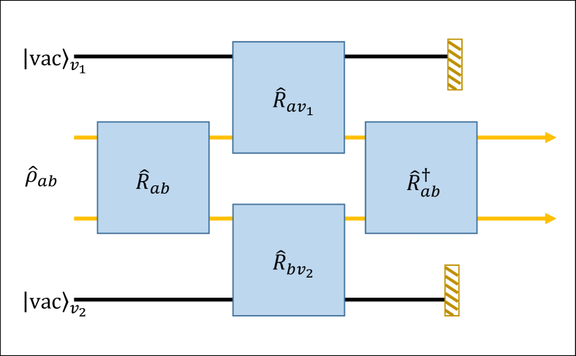
Figure 3: Quantum circuit diagram underlying classical polarization diattenuations. The input polarization state $\hat{\rho}_{ab}$ is first rotated to a desired configuration, the two modes are each attenuated via a rotation with their auxiliary vacuum modes $v_{1}$ and $v_{2}$, the vacuum modes are ignored, the polarization modes are rotated back to the original configuration, and the output two arrows correspond to the diattenuated polarization state.

The marked difference between polarization rotations and diattenuations is that the former is a unitary transformation on the polarization state and the latter is not, instead given by a quantum channel of the form of Eq. (114) with more than one Kraus operator $\hat{K}_{l}$. Regrettably, the quantum theory refers to unitary channels as deterministic and nonunitary channels as nondeterministic, even though both transformations are classically referred to as deterministic from a polarization standpoint.

It is noteworthy that all of transformations governed by a single Jones matrix, classically referred to as deterministic, can be considered to conserve photon number in some enlarged Hilbert space. We will see this to change when inspecting classically nondeterministic polarization transformations.

III.2.2 Quantum Transformations Underlying Mueller Matrix Calculus

It is straightforward to generalize the quantum transformations underlying “deterministic” polarization transformations to those underlying transformations of the form of Eqs. (28) and (31) with more than one nonzero weight $\lambda_{i}$. Under the standard assumption that the classical weights can only be positive, the quantum transformations immediately follow as probabilistic mixtures of the underlying quantum transformations. These can be seen as the nondeterministic transformations

$$\hat{\rho}\to\sum_{i}\lambda_{i}\sum_{l}\hat{K}_{l}^{(i)}\hat{\rho}\hat{K}_{l}^{(i)\dagger}\quad\Rightarrow\quad\mathbf{M}=\sum_{i}\lambda_{i}\mathbf{M}^{(i)},$$ (118)

where each Mueller matrix $\mathbf{M}^{(i)}$ arises from a deterministic polarization transformation with Kraus operators $\hat{K}_{l}^{(i)}$. The new transformations are now governed by the larger set of Kraus operators $\sqrt{\lambda_{i}}\hat{K}_{l}^{(i)}$, indexed by both $i$ and $l$, which can also be used in Eq. (116) to describe the most general quantum mechanical transformation on the Stokes operators that leads to Mueller matrix transformations of the Stokes parameters.

Many examples serve to tease apart the nuances of quantum polarization transformations. For example, consider a classical transformation whereby a state has an equal probability of undergoing one of two rotations parametrized as $\mathbf{R}_{i}=\mathbf{R}\left(\Theta_{i},\mathbf{n}_{i}\right)$. Quantum mechanically, this may arise by a unitary operation between a polarization state $\lvert\psi\rangle_{ab}$ and an auxiliary mode initially in its vacuum state as

$$\lvert\psi\rangle_{ab}\otimes\lvert 0\rangle_{v}\to\frac{\hat{R}_{1}\lvert\psi\rangle_{ab}\otimes\lvert 1\rangle_{v}+\hat{R}_{2}\lvert\psi\rangle_{ab}\otimes\lvert 2\rangle_{v}}{\sqrt{2}}.$$ (119)

Since the amount of rotation becomes entangled with the auxiliary mode, which may have gone a photon-number nonconserving operation, ignoring the vacuum mode leads to the effective polarization transformation

$$\hat{\rho}_{ab}\to\frac{1}{2}\hat{R}_{1}\hat{\rho}\hat{R}_{1}^{\dagger}+\frac{1}{2}\hat{R}_{2}\hat{\rho}\hat{R}_{2}^{\dagger}.$$ (120)

This is equivalent to a transformation with the pair of Kraus operators $\hat{K}_{i}=\hat{R}_{i}/\sqrt{2}$ that manifestly satisfy the normalization requirement of Eq. (114). Even though this operation is unitary in a larger Hilbert space, it is markedly different from the simple rotation transformations that enact diattenuations in larger Hilbert spaces.

III.2.3 Speculative Constraints on Polarization Changes

Quantum channels acting on a quantum state must be completely positive. A general further assumption is that they preserve the trace of the quantum state, so as to preserve total probability. How do these considerations, encompassed by Eq. (114), constrain the possible Mueller matrix transformations of Eq. (29)?

We do not yet have an answer to this question. It is clear from the above sections that all classical transformations falling under the assumptions of Section II.3.6 can be reproduced by the quantum theory. Can we justify these assumptions by assuming only quantum theory? Can we circumvent these assumptions using quantum theory? As mentioned before, these questions have been touched on previously by Ahnert and Payne [12], Aiello et al. [13], Sudha et al. [360], Simon et al. [342], Gamel and James [123], but we believe them to remain unanswered.

The linearity assumption is easiest to break, but that can be broken using both classical and quantum perspectives. Namely, many transformations ascribing to the form of Eq. (116) do not lead to linear transformations among the Stokes parameters; an easy example is a unitary operation corresponding to a nonlinear Hamiltonian, such as

$$\hat{U}=\exp\left(-\text{i}\chi\hat{S}_{3}^{2}\right).$$ (121)

Similarly, not all classical transformations are linear, as with light experiencing the Kerr effect, so we should not expect every operation in the universe to produce a transformation with a Mueller matrix as in Eq. (29). In fact, nonlinear polarimetry is a field unto itself that merits its own attention [42, 66, 320, 322, 228]. These considerations let us refine our current questions to ask whether quantum considerations affect the constraints of classical linear polarization transformations that are simply governed by Mueller matrices as in Eq. (29).

The most tantalizing question is whether quantum transformations alone can be used to restrict the weights in Eqs. (28) and (31) to be positive, as conjectured by Goldberg [144]. Quantum transformations restricted to the single-photon subspace automatically necessitate the positivity assumption [123], so our conjecture would be proven if one could prove that all quantum transformations that enforce linear transformations among the Stokes parameters must necessarily take single-photon states to single-photon states, but we have already seen that diattenuations do not maintain a single photon-number subspace. Similarly, our conjecture could be proven if one could show that the only quantum transformations that enable linear transformations among the extended Stokes parameters of Eq. (54) are those that enact linear transformations among the regular Stokes parameters. It would be nice to use the SU(4)–O⁺(6) homomorphism discussed in the classical context of Cloude [95] to attack this problem from a quantum standpoint, but not all Mueller matrices are unitary, so there indeed remains work to be done.

We can also continue our classical discussion of the restriction on Mueller matrices to satisfy the transmittance and reverse transmittance conditions. It is evident that two Kraus operators $\hat{K}_{1}=\mathbf{J}_{1}$ and $\hat{K}_{2}=\mathbf{J}_{2}$ expressed in the single-photon basis as in Eq. (59) lead to the transformation

$$\hat{\rho}_{\mathrm{single\,photon}}\to\sum_{l=1}^{2}\hat{K}_{l}\hat{\rho}_{\mathrm{single\,photon}}\hat{K}_{l}^{\dagger}=\lvert 1\rangle_{\mathrm{R}}\langle 1\rvert\otimes\lvert 0\rangle_{\mathrm{L}}\langle 0\rvert.$$ (122)

Somehow, there exists a quantum mechanical transformation that leads to the Mueller matrix of Eq. (58), when restricted to act on single-photon input states, that violates the reverse transmittance condition. Have we uncovered a contradiction between the theories?

As with all paradoxes in the technical sense of the word, a resolution awaits. The creation of such an input-agnostic polarization transformer from linear optical devices requires postselection to enable a lossless polarizer [408]; in actuality, some light is always lost by such a polarizer. Such a transformation with Kraus operators enacting Eq. (122) certainly exists, because it is always possible to create a quantum channel on a finite-dimensional Hilbert space that takes arbitrary input states to a fixed output state [401], but it raises concerns that we presently address: What about infinite-dimensional input states? Is this transformation really linear?

One can concoct a quantum channel that transforms arbitrary input states into a given pure output state $\lvert\psi_{\mathrm{target}}\rangle$ by amassing an infinite set of Kraus operators that transform a complete set of basis states into the desired final state:

$$\hat{K}_{m,n}=\lvert\psi_{\mathrm{target}}\rangle\langle m,n\rvert,\qquad\forall\,m,n\in\left(0,1,\cdots,\infty\right).$$ (123)

These Kraus operators readily satisfy the normalization constraint of Eq. (114) and so represent a viable physical transformation; similar results can be obtained if the target state is mixed [401]. However, such a channel does not enact a linear transformation among the Stokes parameters, as it creates output states with the same total intensity regardless of the input intensity. We can modify this scheme to create an ideal lossless polarizer that polarizes all input light into the direction $\Omega$ by using the infinite set of Kraus operators

$$\hat{K}_{m,n}=\lvert\Omega^{(m+n)}\rangle\langle m,n\rvert,\qquad\forall\,m,n\in\left(0,1,\cdots,\infty\right),$$ (124)

which again satisfies all of the requirements of a quantum channel. This appears to act linearly, as it directly enacts a Mueller matrix with the form of Eq. (58):

$$\mathbf{M}=\begin{pmatrix}1&\mathbf{0}^{\top}\\ \mathbf{n}_{\Omega}&\mathbf{0}\mathbf{0}^{\top}\end{pmatrix}$$ (125)

(as a reminder, the outer product $\mathbf{0}\mathbf{0}^{\top}$ equals a $3\times 3$ matrix of zeroes). Quantum theory here contradicts the standard assumptions of classical polarization theory.

For many reasons, one should not expect transformations with Kraus operators such as those in Eqs. (123) and (124) to ever be feasible in practice. The Kraus operators can be physically interpreted as a measure-and-prepare operation that checks what the input state is and outputs some state depending on that input. Currently, Kraus operators as in Eq. (124) must measure the intensity of the input state and coherently output a perfectly polarized state with that same intensity in order to act like a lossless polarizer. Such a measurement process alone is unlikely to be linear, but an even greater challenge is to create a physical setup that can enact this transformation for arbitrary input intensities (and, likewise, arbitrary superpositions and convex combinations of intensities). Additionally, when considering these Kraus operators as arising from a unitary operation in an enlarged Hilbert space, the unitary must necessarily create a different output state when the initial state of the auxiliary system $v$ is different. For example, the single-photon transformation from Eq. (122) must be constructed from a unitary of the form

$$\hat{U} =\lvert R\rangle\langle R\rvert\otimes\lvert 0\rangle_{v}\langle 0\rvert+\lvert R\rangle\langle L\rvert\otimes\lvert 1\rangle_{v}\langle 0\rvert+\lvert L\rangle\langle R\rvert\otimes\lvert 0\rangle_{v}\langle 1\rvert+\lvert L\rangle\langle L\rvert\otimes\lvert 1\rangle_{v}\langle 1\rvert,\,\mathrm{or}$$ (126)

$$\hat{U} =\lvert R\rangle\langle R\rvert\otimes\lvert 0\rangle_{v}\langle 0\rvert+\lvert R\rangle\langle L\rvert\otimes\lvert 1\rangle_{v}\langle 0\rvert+\lvert L\rangle\langle L\rvert\otimes\lvert 0\rangle_{v}\langle 1\rvert+\lvert L\rangle\langle R\rvert\otimes\lvert 1\rangle_{v}\langle 1\rvert,$$

up to a relabelling of the auxiliary mode. This performs the correct transformation on $\hat{\rho}_{\mathrm{single\,photon}}\otimes\lvert 0\rangle_{v}\langle 0\rvert$, sending it to a right-handed circularly polarized state, while doing the opposite to $\hat{\rho}_{\mathrm{single\,photon}}\otimes\lvert 1\rangle_{v}\langle 1\rvert$, sending it to a left-handed circularly polarized state, so the device would have to be reset each time to ensure the proper input state in the auxiliary system. The infeasibility of such operations is then a quantum justification for the polarization transmittance conditions that are classically assumed. Future work could certainly bolster this connection, which we have only here begun to undertake.

IV Quantum Polarimetry from the Perspective of Quantum Estimation Theory

The crux of polarimetry is the ability to measure polarization and its changes well. There has been significant research showing that techniques from or inspired by quantum theory can be used to outperform their classical counterparts for particular tasks in sensing and metrology [79, 112, 281, 138, 46, 368, 188, 365, 375, 241], so quantum polarimetry offers the potential for similar quantum advantages. Polarimetry tasks have been explored directly from a quantum perspective in a variety of guises that we presently review.

IV.1 Quantum Fisher Information

A central quantity in quantum sensing applications is the quantum Fisher information matrix (QFIM), which characterizes how sensitive a given probe state is to changes in the parameters being measured. The QFIM differs from its classical counterpart in that it is optimized over all possible measurement strategies such that it depends only on the probe state and the parameters being measured. This facilitates a direct search for the most sensitive probe states, which can be used to produce estimates of the underlying parameters with the lowest possible uncertainties.

We start with a few properties of QFIMs [271, 299, 372, 362, 67, 239, 340, 14, 302, 107, 240]. Given a series of of parameters to be estimated $\pmb{\theta}$, we wish to find as small as possible of a covariance matrix for an estimator $\tilde{\pmb{\theta}}$

$$\mathop{\mathrm{Cov}}\nolimits\left(\tilde{\pmb{\theta}}\right)=\langle\left(\tilde{\pmb{\theta}}-\pmb{\theta}\right)\left(\tilde{\pmb{\theta}}-\pmb{\theta}\right)^{\top}\rangle,$$ (127)

where we have assumed unbiased estimators such that

$$\langle\tilde{\pmb{\theta}}\rangle=\pmb{\theta}.$$ (128)

Then, the pivotal result from quantum estimation theory is that the covariance matrix for a measurement repeated $\nu\gg 1$ times is bounded from below by the inverse of the QFIM through the quantum Cramér-Rao bound (qCRB):

$$\mathop{\mathrm{Cov}}\nolimits\left(\tilde{\pmb{\theta}}\right)\geq\nu^{-1}\mathbf{Q}\left(\pmb{\theta};\hat{\rho}_{\pmb{\theta}}\right)^{-1}.$$ (129)

The QFIM is computed from the evolved probe state $\hat{\rho}_{\pmb{\theta}}$ as

$$Q_{ij}\left(\pmb{\theta};\hat{\rho}_{\pmb{\theta}}\right)=\mathop{\mathrm{Tr}}\nolimits\left(\hat{\rho}_{\pmb{\theta}}\frac{\left\{\hat{L}_{\theta_{i}},\hat{L}_{\theta_{j}}\right\}}{2}\right),$$ (130)

where the symmetric logarithmic derivative operators are implicitly defined through

$$\frac{\partial\hat{\rho}_{\pmb{\theta}}}{\partial\theta_{i}}=\frac{\left\{\hat{L}_{\theta_{i}},\hat{\rho}_{\pmb{\theta}}\right\}}{2}$$ (131)

and we are using the anticommutator $\left\{A,B\right\}=AB+BA$. For pure probe states with unitary generators

$$\frac{\partial\hat{\rho}_{\pmb{\theta}}}{\partial\theta_{i}}=\text{i}\left[\hat{\rho}_{\pmb{\theta}},\hat{G}_{i}\right]$$ (132)

the QFIM takes the particularly simple form

$$Q_{ij}\left(\pmb{\theta};\hat{\rho}_{\pmb{\theta}}\right)=4\mathop{\mathrm{Cov}}\nolimits_{\hat{\rho}_{\pmb{\theta}}}\left(\hat{G}_{i},\hat{G}_{j}\right),$$ (133)

where we are using the symmetrized covariance $\mathop{\mathrm{Cov}}\nolimits_{\hat{\rho}}\left(A,B\right)=\langle\left\{A,B\right\}\rangle/2-\langle A\rangle\langle B\rangle$ that takes expectation values with respect to state $\hat{\rho}$. When there is a single parameter $\theta$ to be estimated, the qCRB of Eq. (129) is always saturable. For multiparameter estimation, the bound is saturable when, for all $i$ and $j$,

$$\mathop{\mathrm{Tr}}\nolimits\left(\hat{\rho}_{\pmb{\theta}}\left[\hat{L}_{\theta_{i}},\hat{L}_{\theta_{j}}\right]\right)=0.$$ (134)

Many other details about quantum estimation can be found in the above-mentioned reviews and we, further, draw attention to recent work investigating situations in which the QFIM in Eq. (129) cannot be inverted or changes discontinuously [388, 149, 409, 332, 404, 153].

IV.2 Rotation Measurements

IV.2.1 Phase Estimation

One main quantum-enhanced measurement protocol is mathematically equivalent to a subset of rotation measurements: phase estimation. Many physical processes amount to estimating a single parameter $\theta$ from a unitary of the form $\hat{U}=\exp\left(-\text{i}\theta\hat{G}\right)$. In the language of polarization, this arises when trying to estimate the angle of a polarization rotation about a known axis such as $\mathbf{n}=\mathbf{e}_{3}$:

$$\hat{U}(\theta)=\hat{R}\left(\theta,\mathbf{z}\right)=\exp\left(-\text{i}\theta\hat{S}_{3}\right).$$ (135)

Using a classical state for such an estimation problem leads to the evolution

$$\lvert\psi_{\mathrm{classical}}(\theta)\rangle=\hat{U}(\theta)\left(\lvert\alpha\rangle_{\mathrm{R}}\otimes\lvert 0\rangle_{\mathrm{L}}\right)=\lvert\alpha\text{e}^{-\text{i}\frac{\theta}{2}}\rangle_{\mathrm{R}}\otimes\lvert 0\rangle_{\mathrm{L}}.$$ (136)

We can compute the QFIM as a function of the average photon number (i.e., energy) of the input light

$$H=\langle\hat{N}\rangle$$ (137)

to find the “shot-noise-scaling” QFIM

$$Q\left(\theta;\lvert\psi_{\mathrm{classical}}\rangle\right)=H.$$ (138)

A NOON state such as that of Eq. (95) with $\Theta=0$ is much more sensitive, evolving as

$$\lvert\psi_{\mathrm{NOON}}(\theta)\rangle=\hat{U}(\theta)\frac{\lvert N,0\rangle+\lvert 0,N\rangle}{\sqrt{2}}=\frac{\text{e}^{-\text{i}\frac{\theta}{2}}\lvert N,0\rangle+\text{e}^{\text{i}\frac{\theta}{2}}\lvert 0,N\rangle}{\sqrt{2}}.$$ (139)

This leads to a “Heisenberg-scaling” QFIM

$$Q\left(\theta;\lvert\psi_{\mathrm{NOON}}\rangle\right)=H^{2},$$ (140)

allowing for much more sensitive measurements than the classical scheme with a commensurate amount of input energy.

This advantage in phase estimation is readily extendible to simultaneously estimating multiple phases [188]. There, an additional advantage is seen versus the sequential estimation of each of the parameters. Caveats exist in terms of the availability of a reference mode [198, 146] and the number of required measurements [160], but we cannot consider generalized polarimetry to be a multiphase estimation protocol because the polarimetric parameters are not all mutually independent. Instead, we continue to investigate quantum-enhanced polarimetry along the standard decompositions of polarization transformations.

IV.2.2 Rotations about Unknown Axes

A more intricate estimation problem is that of estimating both the rotation angle and rotation axis of an unknown rotation. This has been done using a variety of parametrizations for the three parameters of a rotation [40, 149, 121, 180, 152], which can all be unified from a geometrical perspective [154].

No matter the parametrization of the triad of rotation parameters $\pmb{\theta}$, rotation operations are unitary, per Eq. (105). This facilitates three unitary generators of the transformation

$$\hat{G}_{i}=\text{i}\frac{\partial\hat{R}\left(\pmb{\theta}\right)}{\partial\theta_{i}}\hat{R}^{\dagger}\left(\pmb{\theta}\right),$$ (141)

one for each parameter $\theta_{i}$. Since these can be shown to be comprised from linear combinations of Stokes operators [152, 154], in the form of

$$\hat{G}_{i}=\mathbf{g}\cdot\mathbf{S},$$ (142)

they can readily be computed using any representation of SU(2), which is especially straightforward using Pauli matrices. The QFIM then takes the form

$$\mathbf{Q}\left(\pmb{\theta};\psi\right)=4\mathbf{G}\left(\pmb{\theta}\right)^{\top}\mathbf{C}\left(\psi_{\pmb{\theta}}\right)\mathbf{G}\left(\pmb{\theta}\right),\quad\mathbf{G}=\begin{pmatrix}\mathbf{g}_{1}&\mathbf{g_{2}}&\mathbf{g}_{3}\end{pmatrix},\quad\mathbf{C}_{ij}\left(\psi\right)=\mathop{\mathrm{Cov}}\nolimits_{\lvert\psi\rangle\langle\psi\rvert}\left(\hat{S}_{i},\hat{S}_{j}\right),$$ (143)

which, by rotating the covariance matrix to that of the unrotated state via $\mathbf{C}\left(\psi_{\pmb{\theta}}\right)=\mathbf{R}\left(\pmb{\theta}\right)^{\top}\mathbf{C}\left(\psi\right)\mathbf{R}\left(\pmb{\theta}\right)$, allows us to fully separate the parametric dependence of the QFIM from its state dependence:

$$\mathbf{Q}\left(\pmb{\theta};\psi\right)=4\pmb{G}\left(\pmb{\theta}\right)^{\top}\mathbf{C}\left(\psi\right)\pmb{G}\left(\pmb{\theta}\right),\quad\pmb{G}=\mathbf{R}\mathbf{G}.$$ (144)

This allows one to maximize the “sensitivity covariance matrix” over all probe states $\lvert\psi\rangle$ without having to worry about the absolute values of the parameters or the parametrization being considered.

The qCRB of Eq. (129) is a matrix bound, which is hard to uniquely optimize. A scalar bound can be found by using a positive-definite weight matrix $\mathbf{W}$ to produce the lower bound for a certain linear combination of the parameters’ variances and covariances

$$\mathop{\mathrm{Tr}}\nolimits\left[\mathbf{W}\mathop{\mathrm{Cov}}\nolimits\left(\tilde{\pmb{\theta}},\tilde{\pmb{\theta}}^{\top}\right)\right]\geq\mathop{\mathrm{Tr}}\nolimits\left[\mathbf{W}\mathbf{Q}\left(\pmb{\theta};\hat{\rho}_{\pmb{\theta}}\right)^{-1}\right].$$ (145)

When the weight matrix is chosen to be the metric tensor for SU(2), $\mathbf{W}=\bm{\eta}$, all of the matrices $\pmb{G}$ cancel and we are left with the scalar qCRB for the weighted mean-square error wMSE [154]

$$\mathrm{wMSE}(\tilde{\pmb{\theta}})=\mathop{\mathrm{Tr}}\nolimits\left[\bm{\eta}\mathop{\mathrm{Cov}}\nolimits\left(\tilde{\pmb{\theta}},\tilde{\pmb{\theta}}^{\top}\right)\right]\geq\mathop{\mathrm{Tr}}\nolimits\left[\mathbf{C}\left(\psi\right)^{-1}\right].$$ (146)

This can then be uniquely optimized to find the most sensitive probe states for simultaneously estimating all three parameters of a rotation.

Probe states with the smallest values of $\mathrm{wMSE}(\tilde{\pmb{\theta}})$ for a given average energy $H$ have a few properties [149, 150, 152, 154]:

• They are pure states

• They have definite total spin $S_{0}=H/2$.

• They are classically unpolarized ($p=0$), meaning that the Stokes operators have vanishing expectation value $\hat{\mathbf{S}}=\mathbf{0}$.

• They are unpolarized to second order, making them anticoherent states or Kings of Quantumness to second order, with isotropic sensitivity covariance matrices $\mathbf{C}\left(\psi\right)\propto\mathds{1}$.

The tetrahedral state given in Fig. 2 is an example of such an ideal probe state, with other examples also having highly symmetric Majorana constellations. They achieve the Heisenberg-scaling lower bound

$$\mathrm{wMSE}(\tilde{\pmb{\theta}})\geq 4\frac{9}{H\left(H+1\right)},$$ (147)

which can be saturated by an optimal measurement scheme [152]. NOON states, by contrast, only have symmetries about a single axis in their Majorana constellations, so they are no longer superior in rotation estimation, instead achieving only shot-noise scaling

$$\mathrm{wMSE}(\tilde{\pmb{\theta}})\geq 4\frac{2H+1}{H^{2}}.$$ (148)

Such ideal second-order unpolarized states have been generated using light’s orbital angular momentum degree of freedom [61] and work is underway to do likewise in the polarization degrees of freedom.

The qCRB is saturable for the simultaneous estimation of all three rotation parameters for all pure unpolarized states. This is in stark contrast to classical light, which we saw in Eqs. (71) and (72) to obey stricter inequalities due to them violating the commutativity condition of Eq. (134) [197]. The nature of the optimal detection scheme for a given probe state thereby depends on the polarization properties of the probe, with the ultimate limit being achieved by second-order unpolarized states of light.

IV.3 Diattenuation Measurements

It is also possible to obtain quantum enhancements in diattenuation measurements. These are physically equivalent to transmission and absorption measurements, which have been shown to benefit from quantum enhancements [194, 176, 172, 284, 65, 200, 6, 16, 101, 274, 294, 246, 190]; however, these enhancements are modest, as they do not allow for improved scaling with probe energy beyond the shot-noise limit.

IV.3.1 Attenuation

As described above, attenuation enacts the input-output relation

$$\hat{a}\to\sqrt{q}\hat{a}+\sqrt{1-q}\hat{v},$$ (149)

where mode $a$ is being attenuated and mode $v$ is initially in its vacuum state. This evolution also governs absorption, reflection, and transmission measurements, all of which seek to estimate $q$ or a related parameter. A canonical coherent state evolves as

$$\lvert\alpha\rangle\to\lvert\sqrt{q}\alpha\rangle=\text{e}^{\left(1-q\right)\left|\alpha\right|^{2}/2}q^{\hat{a}^{\dagger}\vphantom{a}\hat{a}/2}\lvert\alpha\rangle,$$ (150)

yielding the QFIM

$$Q(q;\lvert\alpha\rangle)=\frac{H}{q},\quad H=\left|\alpha\right|^{2}.$$ (151)

The optimal quantum strategy, by contrast, uses Fock states $\lvert N\rangle$ that evolve as

$$\lvert N\rangle\langle N\rvert\to\sum_{k=0}^{N}\binom{N}{k}q^{k}\left(1-q\right)^{N-k}\lvert k\rangle\langle k\rvert.$$ (152)

The coefficients in this probability distribution take the same form as for SU(2)-coherent states in Eq. (82) because attenuations are akin to rotations with an ignored auxiliary mode. Fock states have the improved QFIM

$$Q(q;\lvert N\rangle)=\frac{H}{q\left(1-q\right)},$$ (153)

which is especially helpful in the limit of small losses $q\approx 1$. No enhanced scaling with $H$ is possible, so the improvements are not as dramatic as for enhanced rotation sensing and can equally be achieved with $N$ single-photon states or a single $N$-photon state. This has been demonstrated with single photons heralded using spontaneous parametric downconversion [402, 68, 288, 319, 318, 393, 405].

Practically speaking, it is often easier to create two-mode squeezed vacuum (TMSV) states of the form

$$\lvert\psi_{\mathrm{TMSV}}\rangle=\frac{1}{\cosh\zeta}\sum_{N=0}^{\infty}\left(-\text{e}^{\text{i}\varphi}\tanh\zeta\right)^{N}\lvert N,N\rangle,$$ (154)

with average energy $H=2\sinh^{2}\zeta$, than Fock states $\lvert N\rangle$. In fact, this is what is generated via spontaneous parametric downconversion when no heralding is performed. These states evolve as

$$\lvert\psi_{\mathrm{TMSV}}\rangle\langle\psi_{\mathrm{TMSV}}\rvert\to\sum_{m=0}^{\infty}\left(1-q\right)^{m}\lvert\psi_{m}\rangle\langle\psi_{m}\rvert$$ (155)

for the mutually orthogonal, unnormalized states

$$\lvert\psi_{m}\rangle=\frac{1}{\cosh\zeta}\sum_{N=0}^{\infty}\sqrt{\binom{N+m}{m}}\left(-\text{e}^{\text{i}\varphi}\sqrt{q}\tanh\zeta\right)^{N}\lvert N,N+m\rangle.$$ (156)

TMSV states have the same QFIM as Fock states to lowest order in $H$, making them similarly useful in the limit of small $q$ and small $H$ for providing quantum advantages, which has indeed been demonstrated [364, 353, 105, 338, 27].

IV.3.2 Diattenuation

The estimation of two attenuation factors for orthogonal modes can simply consist of two parallel single attenuation measurements. Seeing that a Fock state $\lvert N\rangle$ is optimal for sensing a single attenuation parameter $q$, a pair of Fock states is ideal for measuring a pair of attenutation parameters:

$$\mathbf{Q}\left(q,r;\lvert N_{1},N_{2}\rangle\right)=H\begin{pmatrix}\frac{h_{1}}{q\left(1-q\right)}&0\\ 0&\frac{h_{2}}{r\left(1-r\right)}\end{pmatrix},$$ (157)

where $h_{i}=N_{i}/\left(N_{1}+N_{2}\right)$ is the energy fraction in each mode. This is a special sort of quantum probe state that is only partially polarized with degree of polarization $p=\left|h_{1}-h_{2}\right|$, in contrast to a fully polarized classical probe state that achieves

$$\mathbf{Q}\left(q,r;\lvert\alpha_{\Omega}\rangle\right)=H\begin{pmatrix}\frac{\cos^{2}\Theta}{q}&0\\ 0&\frac{\sin^{2}\Theta}{r}\end{pmatrix}.$$ (158)

One could, in theory, use a pair of TMSV states to measure two attenuation parameters in parallel. This, however, presents physical challenges because the two polarization modes being attenuated are in the same spatial mode, making it difficult to entangle each polarization mode with a different external mode. In this multiparameter context, it is possible to directly use a single TMSV state to measure diattenuation, where the two modes are the polarization modes being attenuated. We have not found this idea directly discussed in the literature, so we briefly sketch such a scheme. A diattenuation of the form of Eq. (113) acting on the two modes of the TMSV leads to the transformation

$$\lvert\psi_{\mathrm{TMSV}}\rangle\langle\psi_{\mathrm{TMSV}}\rvert\to\hat{\varrho}=\sum_{m,n=0}^{\infty}\left(\frac{1-q}{q}\right)^{m}\left(\frac{1-r}{r}\right)^{n}\lvert\psi_{m,n}\rangle\langle\psi_{m,n}\rvert,$$ (159)

$$\qquad\lvert\psi_{m,n}\rangle=\frac{1}{\cosh\zeta}\sum_{N\geq m,n}\left(-\text{e}^{\text{i}\varphi}\sqrt{qr}\tanh\zeta\right)^{N}\sqrt{\binom{N}{m}\binom{N}{n}}\lvert N-m,N-n\rangle.$$

To lowest order in the amount of loss, the QFIM for this evolved state is

$$\mathbf{Q}\left(q,r;\lvert\psi_{\mathrm{TMSV}}\rangle\right)=\frac{H}{2}\begin{pmatrix}\frac{1}{1-q}+\mathcal{O}\left(1\right)&-\frac{3H}{2}-2+\mathcal{O}\left(1-q,1-r\right)\\ -\frac{3H}{2}-2+\mathcal{O}\left(1-q,1-r\right)&\frac{1}{1-r}+\mathcal{O}\left(1\right)\end{pmatrix}.$$ (160)

This evidently performs as well as a pair of Fock states, outperforming coherent states in the small-loss limit, and could readily be used for quantum-enhanced multiparameter diattenuation estimation by taking advantage of the polarization correlations generated by Type II spontaneous parametric downconversion.

IV.4 Combined Measurements

It is not always possible to isolate individual Mueller- or Jones-matrix components for estimation; many realistic scenarios require the simultaneous estimation of, say, rotation and diattenuation parameters. As may be expected, there are tradeoffs in the precision with which each of these parameters may be simultaneously estimated due to different probe states being optimally sensitive for different parameters.

IV.4.1 Phase and Loss

The study of how to achieve quantum enhancements in the simultaneous estimation of two unrelated polarimetry parameters is much younger than its single-parameter counterpart. Crowley et al. [101] first showed that one cannot achieve the ultimate quantum limit in measuring both a rotation angle and an attenuation parameter. Even though the QFIM for estimating these parameters is diagonal, the qCRB is not saturable, precluding an estimate with zero correlation between the two parameters. Perhaps the most disappointing result is that the Heisenberg-scaling performance of phase estimation is overwhelmed by the shot-noise scaling performance of loss estimation in such a scenario for most nonzero values of loss, even when one does not desire to estimate the attenuation parameter [106], due to physical constraints imposed by the Kramers-Kronig relations [131]; this makes quantum-enhanced polarimetry even more of a challenge. The main conclusion is that one has to determine the relative importance of the parameters being estimated in order to best optimize the tradeoffs in their estimation [101]. This type of tradeoff is present in other quantum estimation tasks including the measurment of a phase and a phase diffusion parameter [382, 22, 363, 314]. Possible methods to circumvent these tradeoffs include having the parameters be correlated [51] and using postselection [178].

IV.4.2 Ellipsometry

Until now we have not made any distinction between polarimetry and ellipsometry, as they both investigate polarization properties of the electric field. Ellipsometry typically focuses on determining a specific pair of polarization parameters, namely the ratio between two reflection or transmission components and the difference between two phase shifts, which can be cast as the ratio between two diattenuation parameters $\left(1-q\right)/\left(1-r\right)$ or $q/r$ and a rotation angle about the $\mathbf{e}_{3}$ axis. This has been studied from a few quantum perspectives [3, 4, 373, 374, 161, 317, 390] that we review here. First, one can show that particular quantum states, such as entangled photon pairs, can be used for measuring these two parameters [3, 4, 373, 374, 161, 390]. The QFIM for this measurement has recently been calculated and shown to outperform that of coherent states, especially in the small-absorption regime [390], similar to other attenuation measurement results. Then, the ultimate quantum limit for such a measurement was studied by Rudnicki et al. [317], where it was found that certain squeezed states allow for a simultaneous estimate of both ellipsometry parameters that approaches the Heisenberg limit. This is done by recasting the parameters as eigenvalues of an operator like $\hat{S}_{3}$ and an exponential-of-the-relative-phase operator

$$\hat{E}=\sum_{N}\hat{E}^{(N)},\qquad\hat{E}^{(N)}=\lvert N,0\rangle\langle 0,N\rvert+\sum_{m=0}^{N-1}\lvert m,N-m\rangle\langle m+1,N-m-1\rvert$$ (161)

that serves to shift eigenstates of $\hat{S}_{3}$ by one quantum of angular momentum [251] and finding a probe state that minimizes the uncertainty relation between these two operators. The optimal states in the limit of a large input energy are squeezed vacuum states; for finite energy, the probability distribution of the coefficients $\psi_{m}$ in Eq. (77) is the Fourier transform of a Mathieu function. Such optimal ellipsometric measurements have yet to be performed for large input energies $H$.

IV.4.3 Depolarization

Finally, we mention that estimating the weights $\lambda_{i}$ from a general nondeterministic Mueller matrix stemming from Eq. (31) can never be done with better than shot-noise scaling. This significant result is due to an argument given by Ji et al. [200] relating quantum estimation to programmable quantum channels. Quantum-enhanced polarimetry must therefore be reserved for particular scenarios in which it is worth the cost of preparing special probe states and the ranges of parameters being estimated fall within the appropriate regions discussed above (pure rotations, small loss, etc.).

IV.5 Higher-Order Polarimetry: Measuring Quantum Polarization

No discussion of quantum polarimetry is complete without describing measurements capable of discerning quantum polarization properties about which classical polarimetry is ignorant. A quantum decomposition following the classical form, as given in Eq. (101), is not unique, with $\left(N+1\right)^{2}-4$ remaining degrees of freedom. Similarly, a pure-state decomposition following the classical form

$$\lvert\psi^{(N)}\rangle=\sqrt{p}\lvert\psi_{\mathrm{pol}}^{(N)}\rangle+\text{e}^{\text{i}\varphi}\sqrt{1-p}\lvert\psi_{\mathrm{unpol}}^{(N)}\rangle,\quad\langle\psi_{\mathrm{pol}}^{(N)}\rvert\hat{S}_{\mu}\lvert\psi_{\mathrm{unpol}}^{(N)}\rangle=0$$ (162)

has $2N-7$ remaining parameters after the degree and direction of polarization have been specified. The quantum polarization properties can be arranged in many ways, all of which deal with the extra degrees of freedom present in quantum states beyond the four given by the Stokes parameters.

Quantum tomography can be inspired by classical polarimetry for determining all of the free parameters of a quantum state. By assuming the polarization state to be an arbitrary state of $N$ photons that are not necessarily indistinguishable and thus not necessarily in a symmetric state, measuring the $4^{N}$ generalized Stokes parameters operators

$$\hat{S}_{\mu\nu\cdots\xi}=\sigma_{\mu}\otimes\sigma_{\nu}\otimes\cdots\otimes\sigma_{\xi}$$ (163)

will provide enough information to fully determine the state [196], where we have used a first-quantized notation to delineate the operators acting on each photon as $2\times 2$ Pauli matrices. Linear combinations of these operators may be easier to measure for polarimetry [237], but this does not improve the exponential scaling of the number of measurements required for full tomography. Many other such methods have been proposed using tools from maximum likelihood estimation [185], Bayesian inference [57], and principal component analysis [244], as well as using mutually unbiased bases [234, 315, 215, 5]. The number of measurements to be performed can be reduced using techniques from compressed sensing when the quantum state in question is close to being pure in terms of its matrix rank [164, 100, 243, 333, 120, 242, 203, 34, 355, 311, 62, 130, 136] and these measurements can be done adaptively [10, 11] and have their completeness verified by machine-learning techniques [366]. In practice, overcomplete measurement sets with redundant information tend to be much more useful than minimal measurement sets [77, 410].

The SU(2) symmetry underlying quantum polarization dramatically reduces the number of parameters needed to be estimated for full tomography [265, 103, 371]. Inspecting Eq. (77), for example, the number of free parameters in a pure $N$-photon state is reduced from $2^{N+1}-2$ to $2N$ and in a mixed state from $4^{N}-1$ to $\left(N+1\right)^{2}-1$. This makes the determination of all higher-order polarization properties feasible in practice.

How is quantum polarization best determined? The minimal set of projection operators required for fully determining quantum polarization have been explicitly determined but are challenging to implement experimentally because they require entangled measurements [213]. In an analogous system with SU(2) symmetry, the basis states $\lvert m,N-m\rangle$ can be spatially separated by applying an appropriate magnetic field as in a Stern-Gerlach experiment, facilitating a reconstruction of the quantum state using projectors [103].

$$\hat{P}_{m}=\lvert m,N-m\rangle\langle m,N-m\rvert$$ (164)

Measurement of the projectors can be used to fully determine the properties of a mixed quantum polarization state if one measures these projectors as well as their rotated counterparts for an appropriate set of rotation angles [265]

$$\hat{P}_{m}\left(\pmb{\theta}\right)=\hat{R}\left(\pmb{\theta}\right)\lvert m,N-m\rangle\langle m,N-m\rvert\hat{R}^{\dagger}\left(\pmb{\theta}\right).$$ (165)

This facilitates the experimental reconstruction of the SU(2) Wigner function that completely describes the quantum polarization state [283]. Instead of spatially separating the components $\lvert m,N-m\rangle$, they can be determined by the correlations between the intensities at the two detectors in the SU(2) gadget of Fig. 1, through a scheme that can be traced back to Mukunda and Jordan [290]. First, using the SU(2) gadget with nine specific waveplate orientations allows one to directly measure all of the variances and covariances between the Stokes operators [8]. Next, if only the difference between the intensities at the two detectors is recorded for a sufficient variety of rotation angles, amounting to determining the expectation value of $\hat{P}_{m}(\pmb{\theta})$ summed over all $N\geq m$, a complete polarization tomogram can be constructed [78, 207, 204, 205]. This can also be used to furnish an analysis of a cumulants for the Stokes parameters to arbitrary orders [87], which is another way of arranging the higher-order polarization properties present in a quantums state. Recording all of the intensity correlations for the gadget in Fig. 1 amounts to measuring the expectation values of the correlation operators [327]

$$\hat{W}_{m}=\hat{a}^{\dagger m}\hat{b}^{\dagger N-m}\hat{a}^{m}\hat{b}^{N-m}$$ (166)

that, when rotated appropriately, facilitate a complete reconstruction of the quantum polarization state [192]. The intensity correlations can be directly determined using detectors with sufficient photon-number resolution [41]. Alternatively, one can measure correlations between Stokes operators such as [184]

$$\hat{T}_{l}=\hat{S}_{3}^{l}$$ (167)

and its rotated counterparts, where again the particular sets of sufficient rotations have been studied [118]. These types of correlation measurements allow one to express the quantum polarization properties in a hierarchy of multipole moments [151] that generalizes the according hierarchy in coherence theory [400].

Another method for determining quantum polarization properties is measuring projectors onto SU(2)-coherent states

$$\hat{P}\left(\Omega\right)=\lvert\Omega\rangle\langle\Omega\rvert$$ (168)

and appropriately normalizing the results due to the overcompleteness of these states. This is possible due to the Husimi $Q$-function

$$q(\Omega)=\langle\hat{P}\left(\Omega\right)\rangle$$ (169)

containing complete information about a quantum state [189], which requires obtaining $q(\Omega)$ for a sufficient number of coordinates $\Omega$. For estimating polarization rotations, only four such measurements tend to be necessary [152], while the higher-order quantum polarization properties require $\left(N+1\right)^{2}-1$ measurements along a sufficient set of directions to completely specify the state [179].

The aforementioned compressed sensing techniques can even be used within the symmetric subspace to further enhance the efficiency of quantum polarization measurements for near-pure states [329], with the current state of affairs reviewed by Teo and Sánchez-Soto [367].

We mention in conclusion that the higher-order polarization properties undergo higher-order transformations, leading to objects such as Mueller matrices with dimensions larger than $4\times 4$ [321]. This type of polarimetry could benefit from quantum process tomography and may be useful to understanding high harmonic generation.

V Evaluating Classical Intuitions in Light of Quantum Polarimetry

Armed with a full description of quantum polarization and its transformations, what do we have to say to classical physicists studying polarization? Different nuances are required in different scenarios, so we here highlight a few that we deem most relevant.

V.1 Which Photons are Measured Classically?

No detector measures every photon in an incoming beam of light. Given that the photonic nature underlying classical beams adds extra richness to their polarization properties, how does this affect the outcome of a classical polarization measurement? We here explain that the polarization properties of any subset of photons from a beam of light mimic the polarization properties of the whole beam from a classical standpoint.

We begin by inspecting a general quantum state with some fixed number of photons $N$:

$$\hat{\rho}^{(N)}=\sum_{m,n=0}^{N}\rho_{m,n}^{(N)}\lvert m,N-m\rangle\langle n,N-n\rvert.$$ (170)

Each basis state can be rewritten in a first-quantized description as a symmetric (i.e., permutationally invariant) superposition of single-photon states through

$$\lvert m,N-m\rangle=\frac{1}{\sqrt{\binom{N}{m}}}\sum_{\mathrm{permutations}}\lvert\mathrm{R}\rangle^{\otimes m}\otimes\lvert\mathrm{L}\rangle^{\otimes N-m}.$$ (171)

Then, if a detector only receives $N-1$ of the photons comprising the state, we can describe the state seen by the detector as the result of ignoring one of the permutationally invariant photons, which we set to be the final one for convenience:

$$\hat{\rho}^{(N-1)}=\mathop{\mathrm{Tr}}\nolimits_{\mathrm{one\,photon}}\left(\hat{\rho}^{(N)}\right)=\sum_{\mathrm{X}=\mathrm{R},\mathrm{L}}\langle X\rvert_{N}\hat{\rho}^{(N)}\lvert X\rangle_{N}.$$ (172)

After performing the calculation for each basis state, we find the relationship between the state coefficients to be

$$\rho_{m,n}^{(N-1)}=\frac{\sqrt{\left(N-m\right)\left(N-n\right)}}{N}\rho_{m,n}^{(N)}+\frac{\sqrt{\left(m+1\right)\left(n+1\right)}}{N}\rho_{m+1,n+1}^{(N)},$$ (173)

which may be iterated to find the coefficients for any $\hat{\rho}^{(M)}$ with $0\leq M\leq N$. This immediately yields interesting relationships, such as that obtaining any number of photons from a perfectly polarized or completely isotropic state with definite photon number yields a state with identical properties:

$$\mathop{\mathrm{Tr}}\nolimits_{\mathrm{one\,photon}}\left(\lvert\Omega^{(N)}\rangle\langle\Omega^{(N)}\rvert\right)=\lvert\Omega^{(N-1)}\rangle\langle\Omega^{(N-1)}\rvert,\qquad\mathop{\mathrm{Tr}}\nolimits_{\mathrm{one\,photon}}\left(\hat{\mathds{1}}_{N}\right)=\hat{\mathds{1}}_{N-1}.$$ (174)

Even more, we find that the Stokes parameters for the states remain the same up to the intensity normalization, with [145]

$$\frac{1}{N}\mathop{\mathrm{Tr}}\nolimits\left(\rho_{m,n}^{(N)}\hat{S}_{\mu}\right)=\frac{1}{M}\mathop{\mathrm{Tr}}\nolimits\left(\rho_{m,n}^{(M)}\hat{S}_{\mu}\right);$$ (175)

the degree and direction of any subset $M$ photons from an $N$-photon beam are identical. This is a scenario in which quantum polarization reinforces classical intuition, even though the description of the light seems radically different from the latter. At the extreme of $M=1$, every photon that one examines from a beam with $N$ photons will reproduce the same polarization properties as the whole beam [this was noted for $N=2$ by Dogra et al. [109]].

We can ask the same question when given a beam of light with indeterminate photon number

$$\hat{\rho}=\sum_{N}\rho_{N}\hat{\rho}^{(N)}.$$ (176)

Following immediately from the above results, we learn that, when $\hat{\rho}\to\mathop{\mathrm{Tr}}\nolimits_{\mathrm{one\,photon}}\left(\hat{\rho}\right)$, the Stokes operators transform as

$$S_{\mu}=\sum_{N}\rho_{N}\mathop{\mathrm{Tr}}\nolimits\left(\hat{\rho}^{(N)}\hat{S}_{\mu}\right)\to\sum_{N}\rho_{N}\frac{N-1}{N}\mathop{\mathrm{Tr}}\nolimits\left(\hat{\rho}^{(N)}\hat{S}_{\mu}\right).$$ (177)

When the Stokes parameters within each photon-number subspace have the same direction and degree of polarization, i.e., when

$$\mathop{\mathrm{Tr}}\nolimits\left(\hat{\rho}^{(N)}\hat{S}_{\mu}\right)=Ns_{\mu}$$ (178)

for some $N$-independent constants $s_{\mu}$, the overall direction and degree of polarization will be independent from the subset of photons that one obtains from the entire beam. If, however, the polarization properties are not the same in the different Fock layers, then inspecting $N$ photons will, in general, lead to different polarization properties than inspecting some other number $M$ photons. This forces us to distrust classical polarization properties whenever there is a possibility that different photon-number subspaces are polarized to different amounts or in different directions.

The stark differences between states of light with fixed and indeterminate numbers of photons emphasizes the additional complexities and richness that arise when quantum polarization properties are brought to bear.

V.2 Rotating Unpolarized Light leads to Measurable Changes

In classical optics, all unpolarized states of light are the same, up to specifying the total intensity of the light. Remarkably, this same conclusion does not follow quantum mechanically, even for the quantum states of light deemed to be closest to their classically described counterparts.

To recapitulate, we mentioned in Section III.1.2 that certain unpolarized quantum states of light are completely distinguishable from themselves after undergoing a polarization rotation. This is a marked difference from classically unpolarized light, as classical polarization dictates that unpolarized states do not transform when subject to polarization rotations. Similar discrepancies abound.

One method for obtaining classically unpolarized light is by incoherently mixing two perfectly polarized beams of light with equal intensities and orthogonal polarization components. Quantum mechanically, we similarly find that the state

$$\hat{\rho}=\frac{1}{2}\lvert\Omega^{(N)}\rangle\langle\Omega^{(N)}\rvert+\frac{1}{2}\lvert\Omega_{\perp}^{(N)}\rangle\langle\Omega_{\perp}^{(N)}\rvert$$ (179)

is classically unpolarized, where $\langle\Omega^{(N)}\rvert\Omega_{\perp}^{(N)}\rangle=0$, paralleling the discussion surrounding Eq. (95). However, this state is far from isotropic: the variances of the Stokes parameters are not all the same. Choosing, for example, $\Omega$ to point along the $\mathbf{e}_{3}$ axis, we find

$$\mathop{\mathrm{Var}}\nolimits_{\hat{\rho}}\hat{S}_{1}=\mathop{\mathrm{Var}}\nolimits_{\hat{\rho}}\hat{S}_{2}=\frac{N}{4},\quad\mathop{\mathrm{Var}}\nolimits_{\hat{\rho}}\hat{S}_{3}=\frac{N^{2}}{4},$$ (180)

which is responsible for the suboptimal precision of NOON states in metrology seen in Eq. (148). One might think that this anisotropy arises because the states being mixed in Eq. (179) are not fully classical. However, a similar result arises when two canonical coherent states with orthogonal polarization properties are incoherently mixed:

$$\hat{\rho}=\frac{1}{2}\lvert\alpha_{\Omega}\rangle\langle\alpha_{\Omega}\rvert+\frac{1}{2}\lvert\alpha_{\Omega_{\perp}}\rangle\langle\alpha_{\Omega_{\perp}}\rvert.$$ (181)

Again choosing $\Omega$ to point along the $\pmb{e}_{3}$ axis leads to the anisotropic Stokes parameter variances

$$\mathop{\mathrm{Var}}\nolimits_{\hat{\rho}}\hat{S}_{1}=\mathop{\mathrm{Var}}\nolimits_{\hat{\rho}}\hat{S}_{2}=\frac{\left|\alpha\right|^{2}}{4},\quad\mathop{\mathrm{Var}}\nolimits_{\hat{\rho}}\hat{S}_{3}=\frac{\left|\alpha\right|^{2}\left(1+\left|\alpha\right|^{2}\right)}{4}.$$ (182)

These anisotropies mean that the variance of a Stokes parameter will change if such a classically unpolarized state has its polarization rotated and, further, that mixing a right- with a left-handed circularly polarized beam leads to a different state than mixing a horizontally with a vertically polarized beam. Such information is completely lost in a classical description of polarization and yet these properties are completely discernable in classical polarization experiments. The only method to circumvent such problems is to acquire completely isotropic states of the form of Eq. (98), which may be obtained by the complete depolarization of a beam of light

$$\hat{\rho}\to\int d\pmb{\theta}\,\hat{R}\left(\pmb{\theta}\right)\hat{\rho}\hat{R}\left(\pmb{\theta}\right)^{\dagger}.$$ (183)

These discrepancies can all be attributed to the plethora of quantum states underlying a single classical decomposition of the form of Eq. (24).

V.3 Transformations of the Polarized-Plus-Unpolarized Decomposition

Polarization transformations act linearly on the polarized and unpolarized components in Eqs. (23) and (24). This means that we can inspect the action of all classical polarization transformations on polarized and unpolarized states in vacuo and combine the actions for partially polarized states. We will see here that such a correspondence only works for the quantum decomposition of Eq. (101), even though other decompositions have other strong physical motivations.

We will iterate three possible quantum decompositions underlying the classical one, following Eqs. (101), (162), and more:

$$\mathrm{I:}\,\,\,\lvert\psi\rangle=\sqrt{p}\lvert\psi_{\mathrm{pol}}\rangle+\text{e}^{\text{i}\varphi}\sqrt{p}\lvert\psi_{\mathrm{unpol}}\rangle,\quad\langle\psi_{\mathrm{unpol}}\rvert\hat{S}_{\mu}\lvert_{\mathrm{pol}}\rangle=0,$$ (184)

$$\mathrm{II:}\,\,\,\hat{\rho}=p\hat{\rho}_{\mathrm{pol}}+\left(1-p\right)\hat{\rho}_{\mathrm{unpol}},$$

$$\mathrm{III:}\,\hat{\rho}=p\hat{\rho}_{\mathrm{pol}}+\left(1-p\right)\hat{\rho}_{\mathrm{isotropic}}.$$

Each of these decompositions transforms as expected classically under polarization rotations, in that the polarized component remains polarized in a new direction as per the classical rotation of the Stokes vector, the unpolarized component remains unpolarized, and the degree of polarization remains unchanged. Such agreement will not be seen with other polarization transformations. We can also inspect the minimum number of nonclassical polarization degrees of freedom in each decomposition, which happens in a single $N$-photon subspace, where I, II, and III have $2N-7$, $\left(N+1\right)^{2}-4$, and $0$ remaining degrees of freedom. This points to III best resembling the classical decomposition, but we will see this to not be the case following polarization transformations. Of note, pure, partially polarized states such as $\lvert m,n\rangle$ with $m\neq n$ and $m,n\neq 0$ obey none of the decompositions, so the classical decomposition cannot be taken for granted.

Diattenuation and depolarization transformations, in general, reduce the purity of an input quantum state. This means that the pure-state decomposition I will no longer hold following a general polarization transformation, so we cannot simply say that quantum superpositions underly the classical decompositions into polarized and unpolarized fractions.

Partial attenuation ruins decomposition III. Choosing $q=1$ and a nontrivial value of $r$ for the attenuation of the second mode, an isotropic unpolarized state transforms into

$$\frac{\hat{\mathds{1}}_{N}}{N+1}\quad\underset{r}{\to}\quad\frac{1}{N+1}\sum_{m=0}^{N}\sum_{M=m}^{N}\binom{N-m}{M-m}r^{M-m}\left(1-r\right)^{N-M}\lvert m,M-m\rangle\langle m,M-m\rvert.$$ (185)

The unpolarized component of this state is only isotropic in the vacuum and $M=1$ photon-number subspaces; otherwise, it no longer follows decomposition III. This is why we generally state that only decomposition II, i.e., Eq. (101), may underlie the classical decomposition, even though decomposition III is preferable in terms of degrees of freedom and isotropy properties.

It is clear from the discussion of unpolarized states that decomposition III will also perform poorly for depolarization transformations. For example, we expect a convex combination of a do-nothing operation and rotation by $\pi$ to be able to completely depolarize an incident polarized state:

$$\hat{\rho}_{\mathrm{pol}}\quad\underset{\mathrm{depolarization}}{\to}\quad\frac{1}{2}\hat{\rho}_{\mathrm{pol}}+\frac{1}{2}\hat{R}\left(\pi,\mathbf{n}\right)\hat{\rho}_{\mathrm{pol}}\hat{R}^{\dagger}\left(\pi,\mathbf{n}\right)=\hat{\rho}_{\mathrm{unpol}}\neq\hat{\rho}_{\mathrm{isotropic}},$$ (186)

where $\mathbf{n}$ may be any axis orthogonal to the direction of polarization of $\hat{\rho}_{\mathrm{pol}}$. Other depolarizing transformations do indeed suffice for decomposition III, such as that of complete depolarization

$$\hat{\rho}_{\mathrm{pol}}\quad\underset{\mathrm{complete\,depolarization}}{\to}\quad\int d\pmb{\theta}=\hat{R}\left(\pmb{\theta}\right)\hat{\rho}_{\mathrm{pol}}\hat{R}^{\dagger}\left(\pmb{\theta}\right)=\hat{\rho}_{\mathrm{unpol}}=\hat{\rho}_{\mathrm{isotropic}}.$$ (187)

From these considerations, we see that quantum decompositions I-III may be seen to underly the classical polarization decomposition in certain circumstances, but only the quantum decomposition into first-order polarized and unpolarized fractions, II, transforms correctly under all classical polarization transformations. We are thus faced with two alternatives: give up the privileged status of classical polarization transformations or give up the physical intuition of unpolarized states being isotropic under polarization rotations. Both alternatives are required for the quantum states that have no analogue to the classical decomposition into polarized and unpolarized fractions.

V.4 Higher-Order Correspondences

Quantum polarization dictates that classical polarization properties arise from expectation values of noncommuting operators. Therefore, we should not expect higher-order moments of Stokes parameters to transform classically. The Stokes operators themselves transform classically under rotations, so we will leave those aside in this section.

We elucidate the present discrepancy with the example of a diattenuation along the $\mathbf{e}_{3}$ axis, which leads to the classical and quantum transformation

$$S_{3}\quad\underset{q,r}{\to}\quad\frac{q-r}{2}S_{0}+\frac{q+r}{2}S_{3}.$$ (188)

Squared, we expect a transformation like $S_{3}^{2}\to\left(\frac{q-r}{2}S_{0}+\frac{q+r}{2}S_{3}\right)^{2}$, which is quadratic in the Stokes parameters. Quantum mechanically, however, we must take into account the noncommutativity of the vacuum operators $\left[\hat{v}_{i},\hat{v}_{j}^{\dagger}\right]=\delta_{i,j}$ before tracing out their modes, leading to

$$\hat{S}_{3}^{2}\quad\underset{q,r}{\to}\quad\left(\frac{q-r}{2}\hat{S}_{0}+\frac{q+r}{2}\hat{S}_{3}\right)^{2}+\frac{q\left(1-q\right)}{4}\left(\hat{S}_{0}+\hat{S}_{3}\right)+\frac{r\left(1-r\right)}{4}\left(\hat{S}_{0}-\hat{S}_{3}\right).$$ (189)

This differs from what is expected classically, even though the operators $\hat{S}_{0}$ and $\hat{S}_{3}$ commute. In the limit of strong fields, the terms linear in the Stokes operators may perhaps be neglected and one may be permitted to approximate $\langle\hat{S}_{0}\hat{S}_{3}\rangle\approx S_{0}S_{3}$, but a careful consideration of the diattenuation parameters must be considered in such a case to ensure that the fields remain sufficiently strong.

The deviations from classical predictions are even more pronounced with depolarization transformations of higher-order Stokes parameters. This is because a product of Stokes operators evolving under a Kraus map of the form of Eq. (116) undergoes

$$\hat{S}_{\mu}\hat{S}_{\nu}\to\sum_{l}\hat{K}_{l}^{\dagger}\hat{S}_{\mu}\hat{S}_{\nu}\hat{K}_{l}=\sum_{l,m}\hat{K}_{l}^{\dagger}\hat{S}_{\mu}\hat{K}_{m}^{\dagger}\hat{K}_{m}\hat{S}_{\nu}\hat{K}_{l},$$ (190)

where the operations $\hat{K}_{m}\hat{S}_{\nu}\hat{K}_{l}$ are never guaranteed to equal linear combinations of Stokes operators. In some cases, they do facilitate a decomposition into such linear combinations, but those linear combinations are not the ones predicted classically. One must therefore be leery of all classical polarization transformations calculated with higher-order Stokes parameters and use a quantum formalism for understanding any such process.

VI Conclusions

We have toured quantum polarization and the impacts it has on polarimetry. Along the way, we saw the impacts of quantum polarimetry on its classical counterpart and the possibilities of performing quantum-enhanced polarimetry and quantum polarimetry of manifestly nonclassical properties of light. Light’s polarization continues to be a subject of prime interest to novices and practitioners alike and we suspect more mysteries and features of the theory to be unearthed as we go deeper into the quantum realm.

Acknowledgments: AZG would like to thank Girish Agarwal, José Gil, Khabat Heshami, Daniel James, and Wenlei Zhang for discussions and Luis Sánchez-Soto for insightful comments on the manuscript.

References

- Abdel-Aty et al. [2002] Abdel-Aty, Mahmoud, M Sebawe Abdalla, and A-S F Obada (2002), “Entropy squeezing of a two-mode multiphoton Jaynes-Cummings model in the presence of a nonlinear medium,” Journal of Optics B: Quantum and Semiclassical Optics 4 (2), 134–142.
- Abhyankar and Fymat [1969] Abhyankar, K D, and A. L. Fymat (1969), “Relations between the elements of the phase matrix for scattering,” Journal of Mathematical Physics 10 (10), 1935–1938.
- Abouraddy et al. [2001] Abouraddy, Ayman F, Kimani C. Toussaint, Alexander V. Sergienko, Bahaa E. A. Saleh, and Malvin C. Teich (2001), “Ellipsometric measurements by use of photon pairs generated by spontaneous parametric downconversion,” Optics Letters 26 (21), 1717–1719.
- Abouraddy et al. [2002] Abouraddy, Ayman F, Kimani C. Toussaint, Alexander V. Sergienko, Bahaa E. A. Saleh, and Malvin C. Teich (2002), “Entangled-photon ellipsometry,” Journal of the Optical Society of America B 19 (4), 656–662.
- Adamson and Steinberg [2010] Adamson, R B A, and A. M. Steinberg (2010), “Improving quantum state estimation with mutually unbiased bases,” Physical Review Letters 105, 030406.
- Adesso et al. [2009] Adesso, G, F. Dell’Anno, S. De Siena, F. Illuminati, and L. A. M. Souza (2009), “Optimal estimation of losses at the ultimate quantum limit with non-gaussian states,” Physical Review A 79, 040305.
- Agarwal [1971] Agarwal, G S (1971), “On the state of unpolarized radiation,” Lettere al Nuovo Cimento (1971-1985) 1 (2), 53–56.
- Agarwal and Chaturvedi [2003] Agarwal, G S, and S. Chaturvedi (2003), “Scheme to measure quantum Stokes parameters and their fluctuations and correlations,” Journal of Modern Optics 50 (5), 711–716.
- Agarwal and Puri [1994] Agarwal, G S, and R. R. Puri (1994), “Atomic states with spectroscopic squeezing,” Physical Review A 49, 4968–4971.
- Ahn et al. [2019a] Ahn, D, Y. S. Teo, H. Jeong, F. Bouchard, F. Hufnagel, E. Karimi, D. Koutný, J. Řeháček, Z. Hradil, G. Leuchs, and L. L. Sánchez-Soto (2019a), “Adaptive compressive tomography with no a priori information,” Physical Review Letters 122, 100404.
- Ahn et al. [2019b] Ahn, D, Y. S. Teo, H. Jeong, D. Koutný, J. Řeháček, Z. Hradil, G. Leuchs, and L. L. Sánchez-Soto (2019b), “Adaptive compressive tomography: A numerical study,” Physical Review A 100, 012346.
- Ahnert and Payne [2005] Ahnert, S E, and M. C. Payne (2005), “General implementation of all possible positive-operator-value measurements of single-photon polarization states,” Physical Review A 71, 012330.
- Aiello et al. [2007] Aiello, A, G. Puentes, and J. P. Woerdman (2007), “Linear optics and quantum maps,” Physical Review A 76, 032323.
- Albarelli et al. [2020] Albarelli, F, M. Barbieri, M.G. Genoni, and I. Gianani (2020), “A perspective on multiparameter quantum metrology: From theoretical tools to applications in quantum imaging,” Physics Letters A , 126311.
- Albarelli et al. [2019] Albarelli, Francesco, Jamie F. Friel, and Animesh Datta (2019), “Evaluating the Holevo Cramér-Rao bound for multiparameter quantum metrology,” Physical Review Letters 123, 200503.
- Alipour et al. [2014] Alipour, S, M. Mehboudi, and A. T. Rezakhani (2014), “Quantum Metrology in Open Systems: Dissipative Cramér-Rao Bound,” Physical Review Letters 112, 120405.
- Alodjants and Arakelian [1999] Alodjants, A P, and S. M. Arakelian (1999), “Quantum phase measurements and non-classical polarization states of light,” Journal of Modern Optics 46 (3), 475–507.
- Alodjants et al. [1999] Alodjants, Alexander P, Andrei Yu. Leksin, and Sergei M. Arakelian (1999), “Quantum polarimeter for measurement of nonclassical polarization states of light,” in New Trends in Atomic and Molecular Spectroscopy, Vol. 4060, edited by Gagik G. Gurzadyan and Artashes V. Karmenyan, International Society for Optics and Photonics (SPIE) pp. 63 – 68.
- Alodjants et al. [1998] Alodjants, AP, SM Arakelian, and AS Chirkin (1998), “Polarization quantum states of light in nonlinear distributed feedback systems; quantum nondemolition measurements of the Stokes parameters of light and atomic angular momentum.” Applied Physics B: Lasers & Optics 66 (1).
- Alodzhants et al. [1995] Alodzhants, AP, SM Arakelyan, and AS Chirkin (1995), “Formation of polarization-squeezed states of light in spatially periodic nonlinear-optical media,” Journal of Experimental and Theoretical Physics 81 (1), 34–39.
- Altepeter et al. [2011] Altepeter, Joseph B, Neal N. Oza, Milja Medić, Evan R. Jeffrey, and Prem Kumar (2011), “Entangled photon polarimetry,” Optics Express 19 (27), 26011–26016.
- Altorio et al. [2015] Altorio, Matteo, Marco G. Genoni, Mihai D. Vidrighin, Fabrizia Somma, and Marco Barbieri (2015), “Weak measurements and the joint estimation of phase and phase diffusion,” Physical Review A 92, 032114.
- Andersen and Buchhave [2003] Andersen, Ulrik L, and Preben Buchhave (2003), “Polarization squeezing and entanglement produced by a frequency doubler,” Journal of Optics B: Quantum and Semiclassical Optics 5 (4), S486–S491.
- Anderson and Barakat [1994] Anderson, Donald G M, and Richard Barakat (1994), “Necessary and sufficient conditions for a Mueller matrix to be derivable from a Jones matrix,” Journal of the Optical Society of America A 11 (8), 2305–2319.
- Arecchi et al. [1972] Arecchi, F T, Eric Courtens, Robert Gilmore, and Harry Thomas (1972), “Atomic coherent states in quantum optics,” Physical Review A 6, 2211–2237.
- Atkins and Dobson [1971] Atkins, P W, and J. C. Dobson (1971), “Angular momentum coherent states,” Proceedings of the Royal Society of London A: Mathematical, Physical and Engineering Sciences 321 (1546), 321–340.
- Atkinson et al. [2021] Atkinson, GS, E.J. Allen, G. Ferranti, A.R. McMillan, and J.C.F. Matthews (2021), “Quantum enhanced precision estimation of transmission with bright squeezed light,” Physical Review Applied 16, 044031.
- Azzam [1985] Azzam, R M A (1985), “Beam-splitters for the division-of-amplitude photopolarimeter,” Optica Acta: International Journal of Optics 32 (11), 1407–1412.
- Azzam and Bashara [1977] Azzam, R M A, and N. M. Bashara (1977), Ellipsometry and polarized light (North-Holland Pub. Co.).
- Azzam and De [2003] Azzam, R M A, and A. De (2003), “Optimal beam splitters for the division-of-amplitude photopolarimeter,” Journal of the Optical Society of America A 20 (5), 955–958.
- Azzam [1982] Azzam, RMA (1982), “Division-of-amplitude Photopolarimeter (DOAP) for the Simultaneous Measurement of All Four Stokes Parameters of Light,” Optica Acta: International Journal of Optics 29 (5), 685–689.
- Azzam [2011] Azzam, RMA (2011), “The intertwined history of polarimetry and ellipsometry,” Thin Solid Films 519 (9), 2584 – 2588.
- Bai et al. [2021] Bai, Lele, Xin Wen, Yulin Yang, Lulu Zhang, Jun He, Yanhua Wang, and Junmin Wang (2021), “Quantum-enhanced rubidium atomic magnetometer based on Faraday rotation via 795 nm Stokes operator squeezed light,” Journal of Optics 23 (8), 085202.
- Baldwin et al. [2016] Baldwin, Charles H, Ivan H. Deutsch, and Amir Kalev (2016), “Strictly-complete measurements for bounded-rank quantum-state tomography,” Physical Review A 93, 052105.
- Barakat [1963] Barakat, Richard (1963), “Theory of the coherency matrix for light of arbitrary spectral bandwidth,” Journal of the Optical Society of America 53 (3), 317–323.
- Barakat [1981] Barakat, Richard (1981), “Bilinear constraints between elements of the 4 x 4 Mueller-Jones transfer matrix of polarization theory,” Optics Communications 38 (3), 159 – 161.
- Barakat [1987] Barakat, Richard (1987), “Conditions for the physical realizability of polarization matrices characterizing passive systems,” Journal of Modern Optics 34 (12), 1535–1544.
- Barreiro et al. [2011] Barreiro, S, P. Valente, H. Failache, and A. Lezama (2011), “Polarization squeezing of light by single passage through an atomic vapor,” Physical Review A 84, 033851.
- Bartlett et al. [2021] Bartlett, James, Haiping Hu, and Erhai Zhao (2021), “Illuminating the bulk-boundary correspondence of a non-Hermitian stub lattice with Majorana stars,” Physical Review B 104, 195131.
- Baumgratz and Datta [2016] Baumgratz, Tillmann, and Animesh Datta (2016), “Quantum enhanced estimation of a multidimensional field,” Physical Review Letters 116, 030801.
- Bayraktar et al. [2016] Bayraktar, Ömer, Marcin Swillo, Carlota Canalias, and Gunnar Björk (2016), “Quantum-polarization state tomography,” Physical Review A 94, 020105.
- Bazhenov et al. [1994] Bazhenov, V Yu, O. A. Kulikovskaya, and V. B. Taranenko (1994), “Nonlinear coherent polarimetry for measuring the complex nonlinear index,” Optics Letters 19 (6), 381–383.
- Beduini and Mitchell [2013] Beduini, Federica A, and Morgan W. Mitchell (2013), “Optical spin squeezing: Bright beams as high-flux entangled photon sources,” Physical Review Letters 111, 143601.
- Bengtsson and Życzkowski [2017] Bengtsson, Ingemar, and Karol Życzkowski (2017), Geometry of quantum states: An introduction to quantum entanglement, 2nd ed. (Cambridge University Press).
- Bennett et al. [1992] Bennett, Charles H, Francois Bessette, Gilles Brassard, Louis Salvail, and John Smolin (1992), “Experimental quantum cryptography,” Journal of Cryptology 5 (1), 3–28.
- Berry et al. [2009] Berry, D W, B. L. Higgins, S. D. Bartlett, M. W. Mitchell, G. J. Pryde, and H. M. Wiseman (2009), “How to perform the most accurate possible phase measurements,” Physical Review A 80, 052114.
- Białynicki-Birula [1996] Białynicki-Birula, Iwo (1996), “Photon wave function,” in Progress in Optics, Progress in Optics, Vol. 36, edited by E. Wolf (Elsevier) pp. 245 – 294.
- Białynicki-Birula and Białynicka-Birula [2020] Białynicki-Birula, Iwo, and Zofia Białynicka-Birula (2020), “Three measures of fidelity for photon states,” Physical Review A 102, 042201.
- Billings and Land [1948] Billings, B H, and E. H. Land (1948), “A comparative survey of some possible systems of polarized headlights,” Journal of the Optical Society of America A 38 (10), 819–829.
- Billings [1951] Billings, Bruce H (1951), “A monochromatic depolarizer,” Journal of the Optical Society of America 41 (12), 966–975.
- Birchall et al. [2020] Birchall, Patrick M, Euan J. Allen, Thomas M. Stace, Jeremy L. O’Brien, Jonathan C. F. Matthews, and Hugo Cable (2020), “Quantum optical metrology of correlated phase and loss,” Physical Review Letters 124, 140501.
- Birrittella et al. [2021] Birrittella, Richard J, Jason Ziskind, Edwin E. Hach, Paul M. Alsing, and Christopher C. Gerry (2021), “Optimal spin- and planar-quantum squeezing in superpositions of spin coherent states,” Journal of the Optical Society of America B 38 (11), 3448–3456.
- Björk et al. [2015a] Björk, G, A. B. Klimov, P. de la Hoz, M. Grassl, G. Leuchs, and L. L. Sánchez-Soto (2015a), “Extremal quantum states and their Majorana constellations,” Physical Review A 92, 031801.
- Björk et al. [2012] Björk, G, J. Söderholm, Y.-S. Kim, Y.-S. Ra, H.-T. Lim, C. Kothe, Y.-H. Kim, L. L. Sánchez-Soto, and A. B. Klimov (2012), “Central-moment description of polarization for quantum states of light,” Physical Review A 85, 053835.
- Björk et al. [2015b] Björk, Gunnar, Markus Grassl, Pablo de la Hoz, Gerd Leuchs, and Luis L Sánchez-Soto (2015b), “Stars of the quantum Universe: extremal constellations on the Poincaré sphere,” Physica Scripta 90 (10), 108008.
- Björk et al. [2010] Björk, Gunnar, Jonas Söderholm, Luis L. Sánchez-Soto, Andrei B. Klimov, Iulia Ghiu, Paulina Marian, and Tudor A. Marian (2010), “Quantum degrees of polarization,” Optics Communications 283 (22), 4440 – 4447.
- Blume-Kohout [2010] Blume-Kohout, Robin (2010), “Optimal, reliable estimation of quantum states,” New Journal of Physics 12 (4), 043034.
- Bogdanov et al. [2004] Bogdanov, Yu I, M. V. Chekhova, S. P. Kulik, G. A. Maslennikov, A. A. Zhukov., C. H. Oh, and M. K. Tey (2004), “Qutrit state engineering with biphotons,” Physical Review Letters 93, 230503.
- Bonsma-Fisher et al. [2019] Bonsma-Fisher, Kent A G, Weng-Kian Tham, Hugo Ferretti, and Aephraim M Steinberg (2019), “Realistic sub-Rayleigh imaging with phase-sensitive measurements,” New Journal of Physics 21 (9), 093010.
- Born and Wolf [1999] Born, Max, and Emil Wolf (1999), Principles of optics: Electromagnetic theory of propagation, interference and diffraction of light., 7th ed. (Cambridge University Press).
- Bouchard et al. [2017] Bouchard, Frederic, P de la Hoz, Gunnar Björk, RW Boyd, M Grassl, Z Hradil, E Karimi, AB Klimov, G Leuchs, J Řeháček, and LL Sánchez-Soto (2017), “Quantum metrology at the limit with extremal Majorana constellations,” Optica 4 (11), 1429–1432.
- Bouchard et al. [2019] Bouchard, Frédéric, Dominik Koutný, Felix Hufnagel, Zdeněk Hradil, Jaroslav Řeháček, Yong-Siah Teo, Daekun Ahn, Hyunseok Jeong, Luis L. Sánchez-Soto, Gerd Leuchs, and Ebrahim Karimi (2019), “Compressed sensing of twisted photons,” Optics Express 27 (13), 17426–17434.
- Bouwmeester et al. [1997] Bouwmeester, Dik, Jian-Wei Pan, Klaus Mattle, Manfred Eibl, Harald Weinfurter, and Anton Zeilinger (1997), “Experimental quantum teleportation,” Nature 390, 575.
- Bowen et al. [2002] Bowen, Warwick P, Roman Schnabel, Hans-A. Bachor, and Ping Koy Lam (2002), “Polarization Squeezing of Continuous Variable Stokes Parameters,” Physical Review Letters 88, 093601.
- Brambilla et al. [2008] Brambilla, E, L. Caspani, O. Jedrkiewicz, L. A. Lugiato, and A. Gatti (2008), “High-sensitivity imaging with multi-mode twin beams,” Physical Review A 77, 053807.
- Brasselet and Zyss [2007] Brasselet, Sophie, and Joseph Zyss (2007), “Nonlinear polarimetry of molecular crystals down to the nanoscale,” Comptes Rendus Physique 8 (2), 165–179.
- Braun et al. [2018] Braun, Daniel, Gerardo Adesso, Fabio Benatti, Roberto Floreanini, Ugo Marzolino, Morgan W. Mitchell, and Stefano Pirandola (2018), “Quantum-enhanced measurements without entanglement,” Reviews of Modern Physics 90, 035006.
- Brida et al. [2010] Brida, G, M. Genovese, and I. Ruo Berchera (2010), “Experimental realization of sub-shot-noise quantum imaging,” Nature Photonics 4 (4), 227–230.
- Brif and Mann [1996] Brif, C, and A. Mann (1996), “Nonclassical interferometry with intelligent light,” Physical Review A 54, 4505–4518.
- Brosseau [1998] Brosseau, Christian (1998), Fundamentals of polarized light: a statistical optics approach (Wiley-Interscience).
- Brosseau [2010] Brosseau, Christian (2010), “Polarization and coherence optics: historical perspective, status, and future directions,” Progress in Optics 54, 149–208.
- Brosseau and Barakat [1991] Brosseau, Christian, and Richard Barakat (1991), “Jones and Mueller polarization matrices for random media,” Optics Communications 84 (3), 127 – 132.
- Brosseau and Dogariu [2006] Brosseau, Christian, and Aristide Dogariu (2006), “Symmetry properties and polarization descriptors for an arbitrary electromagnetic wavefield,” Progress in Optics 49, 315.
- Brosseau et al. [1993] Brosseau, Christian, Clark R. Givens, and Alexander B. Kostinski (1993), “Generalized trace condition on the Mueller–Jones polarization matrix,” Journal of the Optical Society of America A 10 (10), 2248–2251.
- Brown [2011] Brown, Thomas G (2011), “Unconventional polarization states: beam propagation, focusing, and imaging,” Progress in Optics 56, 81–129.
- Bruno [2012] Bruno, Patrick (2012), “Quantum Geometric Phase in Majorana’s Stellar Representation: Mapping onto a Many-Body Aharonov-Bohm Phase,” Physical Review Letters 108, 240402.
- de Burgh et al. [2008] de Burgh, Mark D, Nathan K. Langford, Andrew C. Doherty, and Alexei Gilchrist (2008), “Choice of measurement sets in qubit tomography,” Physical Review A 78, 052122.
- Bushev et al. [2001] Bushev, P A, V. P. Karassiov, A. V. Masalov, and A. A. Putilin (2001), “Biphoton light with hidden polarization and its polarization tomography,” Optics and Spectroscopy 91 (4), 526–531.
- Caves [1981] Caves, Carlton M (1981), “Quantum-mechanical noise in an interferometer,” Physical Review D 23, 1693–1708.
- Chabaud et al. [2020] Chabaud, Ulysse, Damian Markham, and Frédéric Grosshans (2020), “Stellar Representation of Non-Gaussian Quantum States,” Physical Review Letters 124, 063605.
- Chakraborty [1986] Chakraborty, Biswajit (1986), “Depolarizing effect of propagation of a polarized polychromatic beam through an optically active medium: a generalized study,” JOSA A 3 (9), 1422–1427.
- Chandrasekhar [1950] Chandrasekhar, S (1950), Radiative Transfer (Clarendon Press).
- Chaturvedi et al. [2006] Chaturvedi, S, G. Marmo, N. Mukunda, R. Simon, and A. Zampini (2006), “The Schwinger Representation of a Group: Concepts and Appplications,” Reviews in Mathematical Physics 18 (08), 887–912.
- Chaudhury et al. [2007] Chaudhury, Souma, Seth Merkel, Tobias Herr, Andrew Silberfarb, Ivan H. Deutsch, and Poul S. Jessen (2007), “Quantum Control of the Hyperfine Spin of a Cs Atom Ensemble,” Physical Review Letters 99, 163002.
- Chirkin [2015] Chirkin, A S (2015), “Polarization-squeezed light and quantum degree of polarization (a review),” Optics and Spectroscopy 119 (3), 371–376.
- Chirkin et al. [1993] Chirkin, Anatolii S, A A Orlov, and D Yu Parashchuk (1993), “Quantum theory of two-mode interactions in optically anisotropic media with cubic nonlinearities: Generation of quadrature- and polarization-squeezed light,” Quantum Electronics 23 (10), 870–874.
- Chirkin and Singh [2021] Chirkin, Anatoly S, and Ranjit Singh (2021), “Quantum polarization characteristic function and cumulant analysis of Stokes parameters,” Journal of Russian Laser Research 42 (6), 658–666.
- Choquette and Leibenguth [1994] Choquette, K D, and R. E. Leibenguth (1994), “Control of vertical-cavity laser polarization with anisotropic transverse cavity geometries,” IEEE Photonics Technology Letters 6 (1), 40–42.
- Chryssomalakos and Hernández-Coronado [2017] Chryssomalakos, C, and H. Hernández-Coronado (2017), “Optimal quantum rotosensors,” Physical Review A 95, 052125.
- Chryssomalakos et al. [2021] Chryssomalakos, Chryssomalis, Louis Hanotel, Edgar Guzmán-González, Daniel Braun, Eduardo Serrano-Ensástiga, and Karol Życzkowski (2021), “Symmetric multiqudit states: Stars, entanglement, and rotosensors,” Physical Review A 104, 012407.
- Civitarese et al. [2013] Civitarese, O, M Reboiro, and D Tielas (2013), “Spin observables in an atomic CQE system,” Journal of Physics B: Atomic, Molecular and Optical Physics 46 (6), 065502.
- Clarke and Grainger [1971] Clarke, D, and JF Grainger (1971), Polarized light and optical measurement, Vol. 1 (Pergamon Press).
- Cloude [1990] Cloude, Shane R (1990), “Conditions for the physical realisability of matrix operators in polarimetry,” .
- Cloude and Pottier [1995] Cloude, Shane R, and Eric Pottier (1995), “Concept of polarization entropy in optical scattering,” Optical Engineering 34 (6), 1599 – 1610.
- Cloude [1986] Cloude, Shane Robert (1986), “Group theory and polarization algebra,” Optik 75 (1), 26–36.
- Collett [1970] Collett, Edward (1970), “Stokes parameters for quantum systems,” American Journal of Physics 38 (5), 563–574.
- Collett [1992] Collett, Edward (1992), Polarized light: Fundamentals and applications (Marcel Dekker, Inc.).
- Collett [2005] Collett, Edward (2005), “Field guide to polarization,” (Spie Bellingham, WA).
- Corney et al. [2008] Corney, Joel F, Joel Heersink, Ruifang Dong, Vincent Josse, Peter D. Drummond, Gerd Leuchs, and Ulrik L. Andersen (2008), “Simulations and experiments on polarization squeezing in optical fiber,” Physical Review A 78, 023831.
- Cramer et al. [2010] Cramer, Marcus, Martin B. Plenio, Steven T. Flammia, Rolando Somma, David Gross, Stephen D. Bartlett, Olivier Landon-Cardinal, David Poulin, and Yi-Kai Liu (2010), “Efficient quantum state tomography,” Nature Communications 1 (1), 149.
- Crowley et al. [2014] Crowley, Philip J D, Animesh Datta, Marco Barbieri, and I. A. Walmsley (2014), “Tradeoff in simultaneous quantum-limited phase and loss estimation in interferometry,” Physical Review A 89, 023845.
- Cui et al. [2013] Cui, Xiaoling, Biao Lian, Tin-Lun Ho, Benjamin L. Lev, and Hui Zhai (2013), “Synthetic gauge field with highly magnetic lanthanide atoms,” Physical Review A 88, 011601.
- D’Ariano et al. [2003] D’Ariano, G M, L Maccone, and M Paini (2003), “Spin tomography,” Journal of Optics B: Quantum and Semiclassical Optics 5 (1), 77–84.
- Daryanoosh et al. [2018] Daryanoosh, Shakib, Sergei Slussarenko, Dominic W. Berry, Howard M. Wiseman, and Geoff J. Pryde (2018), “Experimental optical phase measurement approaching the exact Heisenberg limit,” Nature Communications 9 (1), 4606.
- D'Auria et al. [2006] D'Auria, V, C de Lisio, A Porzio, S Solimeno, and Matteo G A Paris (2006), “Transmittivity measurements by means of squeezed vacuum light,” Journal of Physics B: Atomic, Molecular and Optical Physics 39 (5), 1187–1198.
- Demkowicz-Dobrzanski et al. [2009] Demkowicz-Dobrzanski, R, U. Dorner, B. J. Smith, J. S. Lundeen, W. Wasilewski, K. Banaszek, and I. A. Walmsley (2009), “Quantum phase estimation with lossy interferometers,” Physical Review A 80, 013825.
- Demkowicz-Dobrzański et al. [2020] Demkowicz-Dobrzański, Rafał, Wojciech Górecki, and Mădălin Guţă (2020), “Multi-parameter estimation beyond quantum Fisher information,” Journal of Physics A: Mathematical and Theoretical 53 (36), 363001.
- Dlugnikov [1984] Dlugnikov, LN (1984), “Changes in polarization of a light beam with arbitrary autocoherence propagating in a birefringent crystal,” Optica Acta: International Journal of Optics 31 (7), 803–811.
- Dogra et al. [2020] Dogra, Shruti, Antti Vepsäläinen, and G. S. Paraoanu (2020), “Majorana representation of adiabatic and superadiabatic processes in three-level systems,” Physical Review Research 2, 043079.
- Donati et al. [2014] Donati, Gaia, Tim J. Bartley, Xian-Min Jin, Mihai-Dorian Vidrighin, Animesh Datta, Marco Barbieri, and Ian A. Walmsley (2014), “Observing optical coherence across Fock layers with weak-field homodyne detectors,” Nature Communications 5 (1), 5584.
- Dong et al. [2008] Dong, Ruifang, Joel Heersink, Joel F. Corney, Peter D. Drummond, Ulrik L. Andersen, and Gerd Leuchs (2008), “Experimental evidence for Raman-induced limits to efficient squeezing in optical fibers,” Optics Letters 33 (2), 116–118.
- Dowling [1998] Dowling, Jonathan P (1998), “Correlated input-port, matter-wave interferometer: Quantum-noise limits to the atom-laser gyroscope,” Physical Review A 57, 4736–4746.
- Dulk et al. [1994] Dulk, G A, Y. Leblanc, and A. Lecacheux (1994), “The complete polarization state of Io-related radio storms from Jupiter: A statistical study,” Astronomy and Astrophysics 286, 683–700.
- Espinosa-Luna [2007] Espinosa-Luna, Rafael (2007), “Degree of polarization as a criterion to obtain the nine bilinear constraints between the Mueller-Jones matrix elements,” Applied Optics 46 (24), 6047–6054.
- Falkoff and MacDonald [1951] Falkoff, DL, and JE MacDonald (1951), “On the Stokes parameters for polarized radiation,” JOSA 41 (11), 861–862.
- Fano [1949] Fano, U (1949), “Remarks on the classical and quantum-mechanical treatment of partial polarization,” Journal of the Optical Society of America 39 (10), 859–863.
- Fano [1954] Fano, U (1954), “A Stokes-Parameter Technique for the Treatment of Polarization in Quantum Mechanics,” Physical Review 93, 121–123.
- Filippov and Man’ko [2010] Filippov, Sergey N, and Vladimir I. Man’ko (2010), “Inverse spin-s portrait and representation of qudit states by single probability vectors,” Journal of Russian Laser Research 31 (1), 32–54.
- Firdous and Anwar [2016] Firdous, Shamaraz, and Shahzad Anwar (2016), “Noninvasive optical diagnostic of breast cancer using depolarization of light,” Optik 127 (5), 3035–3038.
- Flammia et al. [2012] Flammia, Steven T, David Gross, Yi-Kai Liu, and Jens Eisert (2012), “Quantum tomography via compressed sensing: error bounds, sample complexity and efficient estimators,” New Journal of Physics 14 (9), 095022.
- Friel et al. [2020] Friel, Jamie, Pantita Palittapongarnpim, Francesco Albarelli, and Animesh Datta (2020), “Attainability of the Holevo-Cramér-Rao bound for two-qubit 3D magnetometry,” arXiv:2008.01502 [quant-ph] .
- Fry and Kattawar [1981] Fry, Edward S, and George W. Kattawar (1981), “Relationships between elements of the Stokes matrix,” Applied Optics 20 (16), 2811–2814.
- Gamel and James [2011] Gamel, Omar, and Daniel F. V. James (2011), “Causality and the complete positivity of classical polarization maps,” Optics Letters 36 (15), 2821–2823.
- Gazeau [2009] Gazeau, Jean-Pierre (2009), Coherent states in quantum physics (Wiley, Weinheim).
- Ge et al. [2012] Ge, Jing Hua, Zhe Chen, Yin Fang Chen, Chun Yan Chen, Yan Fang Zhai, Jun Zhang, Zhan Sui, Hong Huan Lin, Jian Jun Wang, and Qing Hua Deng (2012), “Optimized design of parameters for wedge-crystal depolarizer,” in Mechanical and Aerospace Engineering, ICMAE2011, Applied Mechanics and Materials, Vol. 110 (Trans Tech Publications Ltd) pp. 3351–3357.
- Ghiu et al. [2010] Ghiu, Iulia, Gunnar Björk, Paulina Marian, and Tudor A. Marian (2010), “Probing light polarization with the quantum chernoff bound,” Physical Review A 82, 023803.
- Ghiu et al. [2018] Ghiu, Iulia, Paulina Marian, and Tudor A. Marian (2018), “Modification of polarization through de-gaussification,” Physical Review A 98, 033826.
- Gühne and Tóth [2009] Gühne, Otfried, and Géza Tóth (2009), “Entanglement detection,” Physics Reports 474 (1), 1–75.
- Ghosh et al. [2009] Ghosh, Nirmalya, Michael F. G. Wood, Shu-hong Li, Richard D. Weisel, Brian C. Wilson, Ren-Ke Li, and I. Alex Vitkin (2009), “Mueller matrix decomposition for polarized light assessment of biological tissues,” Journal of Biophotonics 2 (3), 145–156.
- Gianani et al. [2020] Gianani, I, Y.S. Teo, V. Cimini, H. Jeong, G. Leuchs, M. Barbieri, and L.L. Sánchez-Soto (2020), “Compressively certifying quantum measurements,” Physical Review X Quantum 1, 020307.
- Gianani et al. [2021] Gianani, Ilaria, Marco Barbieri, Francesco Albarelli, Adriano Verna, Valeria Cimini, and Rafal Demkowicz-Dobrzanski (2021), “Kramers-Kronig relations and precision limits in quantum phase estimation,” arXiv:2107.10521 arXiv:2107.10521 [quant-ph] .
- Gil and Bernabeu [1985] Gil, José Jorge, and Eusebio Bernabeu (1985), “A Depolarization Criterion in Mueller Matrices,” Optica Acta: International Journal of Optics 32 (3), 259–261.
- Gil [2000] Gil, José J (2000), “Characteristic properties of Mueller matrices,” Journal of the Optical Society of America A 17 (2), 328–334.
- Gil et al. [2013] Gil, José J, Ignacio San José, and Razvigor Ossikovski (2013), “Serial-parallel decompositions of Mueller matrices,” Journal of the Optical Society of America A 30 (1), 32–50.
- Gil, J. J. [2007] Gil, J. J., (2007), “Polarimetric characterization of light and media - physical quantities involved in polarimetric phenomena,” European Physical Journal Applied Physics 40 (1), 1–47.
- Gil-Lopez et al. [2021] Gil-Lopez, J, Y. S. Teo, S. De, B. Brecht, H. Jeong, C. Silberhorn, and L. L. Sanchez-Soto (2021), “Universal compressive tomography in the time-frequency domain,” arXiv:2105.12462 [quant-ph] .
- Gil Pérez and Ossikovski [2016] Gil Pérez, José Jorge Gil, and Razvigor Ossikovski (2016), Polarized light and the Mueller matrix approach (CRC Press).
- Giovannetti et al. [2004] Giovannetti, Vittorio, Seth Lloyd, and Lorenzo Maccone (2004), “Quantum-enhanced measurements: Beating the standard quantum limit,” Science 306 (5700), 1330–1336.
- Giraud et al. [2010] Giraud, Olivier, Petr Braun, and Daniel Braun (2010), “Quantifying quantumness and the quest for Queens of Quantum,” New Journal of Physics 12 (6), 063005.
- Givens and Kostinski [1993] Givens, Clark R, and Alexander B Kostinski (1993), “A simple necessary and sufficient condition on physically realizable Mueller matrices,” Journal of Modern Optics 40 (3), 471–481.
- Glauber [1963a] Glauber, Roy J (1963a), “Coherent and incoherent states of the radiation field,” Physical Review 131, 2766–2788.
- Glauber [1963b] Glauber, Roy J (1963b), “The quantum theory of optical coherence,” Physical Review 130, 2529–2539.
- Goldberg et al. [2021a] Goldberg, A Z, J. L. Romero, Á. S. Sanz, A. B. Klimov, G. Leuchs, and L. L. Sánchez-Soto (2021a), “Random majorana constellations,” arXiv:2112.01612 [quant-ph] .
- Goldberg [2020] Goldberg, Aaron Z (2020), “Quantum theory of polarimetry: From quantum operations to Mueller matrices,” Physical Review Research 2, 023038.
- Goldberg [2021] Goldberg, Aaron Z (2021), Disquisitions on quantum-enhanced polarimetry, Ph.D. thesis.
- Goldberg et al. [2020a] Goldberg, Aaron Z, Ilaria Gianani, Marco Barbieri, Fabio Sciarrino, Aephraim M. Steinberg, and Nicolò Spagnolo (2020a), “Multiphase estimation without a reference mode,” Physical Review A 102, 022230.
- Goldberg et al. [2021b] Goldberg, Aaron Z, Pablo de la Hoz, Gunnar Björk, Andrei B. Klimov, Markus Grassl, Gerd Leuchs, and Luis L. Sánchez-Soto (2021b), “Quantum concepts in optical polarization,” Advances in Optics and Photonics 13 (1), 1–73.
- Goldberg and James [2017] Goldberg, Aaron Z, and Daniel F. V. James (2017), “Perfect polarization for arbitrary light beams,” Physical Review A 96, 053859.
- Goldberg and James [2018] Goldberg, Aaron Z, and Daniel F V James (2018), “Quantum-limited Euler angle measurements using anticoherent states,” Physical Review A 98 (3), 032113.
- Goldberg et al. [2020b] Goldberg, Aaron Z, Andrei B. Klimov, Markus Grassl, Gerd Leuchs, and Luis L. Sánchez-Soto (2020b), “Extremal quantum states,” AVS Quantum Science 2 (4), 044701.
- Goldberg et al. [2021c] Goldberg, Aaron Z, Andrei B. Klimov, Hubert de Guise, Gerd Leuchs, Girish S. Agarwal, and Luis L. Sánchez-Soto (2021c), “From polarization multipoles to higher-order coherences,” arXiv:2109.04474 [quant-ph] .
- Goldberg et al. [2021d] Goldberg, Aaron Z, Andrei B Klimov, Gerd Leuchs, and Luis L Sánchez-Soto (2021d), “Rotation sensing at the ultimate limit,” Journal of Physics: Photonics 3 (2), 022008.
- Goldberg et al. [2021e] Goldberg, Aaron Z, José L. Romero, Ángel S. Sanz, and Luis L. Sánchez-Soto (2021e), “Taming singularities of the quantum Fisher information,” International Journal of Quantum Information 0 (0), 2140004.
- Goldberg et al. [2021f] Goldberg, Aaron Z, Luis L. Sánchez-Soto, and Hugo Ferretti (2021f), “Intrinsic sensitivity limits for multiparameter quantum metrology,” Physical Review Letters 127, 110501.
- Goldstein [2003] Goldstein, Dennis (2003), Polarized light (Dekker, Abingdon).
- Goldstein [1992] Goldstein, Dennis H (1992), “Mueller matrix dual-rotating retarder polarimeter,” Applied Optics 31 (31), 6676–6683.
- Golubev et al. [2004] Golubev, Yu M, T. Yu. Golubeva, M. I. Kolobov, and E. Giacobino (2004), “Polarization squeezing in vertical-cavity surface-emitting lasers,” Physical Review A 70, 053817.
- Gopala Rao et al. [1998a] Gopala Rao, A V, K. S. Mallesh, and Sudha (1998a), “On the algebraic characterization of a Mueller matrix in polarization optics. I. Identifying a Mueller matrix from its N matrix,” Journal of Modern Optics 45 (5), 955–987.
- Gopala Rao et al. [1998b] Gopala Rao, A V, K. S. Mallesh, and Sudha (1998b), “On the algebraic characterization of a Mueller matrix in polarization optics. II. Necessary and sufficient conditions for Jones-derived Mueller matrices,” Journal of Modern Optics 45 (5), 989–999.
- Gorecki and Demkowicz-Dobrzanski [2021] Gorecki, Wojciech, and Rafal Demkowicz-Dobrzanski (2021), “Multiple-phase quantum interferometry – real and apparent gains of measuring all the phases simultaneously,” arXiv:2107.10863 [quant-ph] .
- Graham et al. [2006] Graham, David JL, A. Scott Parkins, and Lionel R. Watkins (2006), “Ellipsometry with polarisation-entangled photons,” Optics Express 14 (16), 7037–7045.
- Grier [2003] Grier, David G (2003), “A revolution in optical manipulation,” Nature 424 (6950), 810–816.
- Gross [2012] Gross, Christian (2012), “Spin squeezing, entanglement and quantum metrology with Bose–Einstein condensates,” Journal of Physics B: Atomic, Molecular and Optical Physics 45 (10), 103001.
- Gross et al. [2010] Gross, David, Yi-Kai Liu, Steven T. Flammia, Stephen Becker, and Jens Eisert (2010), “Quantum state tomography via compressed sensing,” Physical Review Letters 105, 150401.
- Hald et al. [1999] Hald, J, J. L. Sørensen, C. Schori, and E. S. Polzik (1999), “Spin squeezed atoms: A macroscopic entangled ensemble created by light,” Physical Review Letters 83, 1319–1322.
- Hallaji et al. [2017] Hallaji, Matin, Amir Feizpour, Greg Dmochowski, Josiah Sinclair, and Aephraim M. Steinberg (2017), “Weak-value amplification of the nonlinear effect of a single photon,” Nature Physics 13 (6), 540–544.
- Han et al. [2018] Han, Yashuai, Xin Wen, Jinyu Liu, Jun He, and Junmin Wang (2018), “Generation of polarization squeezed light with an optical parametric amplifier at 795 nm,” Optics Communications 416, 1–4.
- Hannay [1998a] Hannay, J H (1998a), “The Berry phase for spin in the Majorana representation,” Journal of Physics A: Mathematical and General 31 (2), L53–L59.
- Hannay [1998b] Hannay, J H (1998b), “The Majorana representation of polarization, and the Berry phase of light,” Journal of Modern Optics 45 (5), 1001–1008.
- Hauge [1976] Hauge, P S (1976), “Survey of methods for the complete determination of a state of polarization,” Proceedings of the SPIE 0088, 3–10.
- Hauge [1980] Hauge, PS (1980), “Recent developments in instrumentation in ellipsometry,” Surface Science 96 (1), 108 – 140.
- Hayat et al. [1999] Hayat, Majeed M, Adel Joobeur, and Bahaa E. A. Saleh (1999), “Reduction of quantum noise in transmittance estimation using photon-correlated beams,” Journal of the Optical Society of America A 16 (2), 348–358.
- He et al. [2011] He, Q Y, Shi-Guo Peng, P. D. Drummond, and M. D. Reid (2011), “Planar quantum squeezing and atom interferometry,” Physical Review A 84, 022107.
- Heersink et al. [2003] Heersink, Joel, Tobias Gaber, Stefan Lorenz, Oliver Glöckl, Natalia Korolkova, and Gerd Leuchs (2003), “Polarization squeezing of intense pulses with a fiber-optic Sagnac interferometer,” Physical Review A 68, 013815.
- Heersink et al. [2005] Heersink, Joel, Vincent Josse, Gerd Leuchs, and Ulrik L. Andersen (2005), “Efficient polarization squeezing in optical fibers,” Optics Letters 30 (10), 1192–1194.
- Heidmann et al. [1987] Heidmann, A, R. J. Horowicz, S. Reynaud, E. Giacobino, C. Fabre, and G. Camy (1987), “Observation of quantum noise reduction on twin laser beams,” Physical Review Letters 59, 2555–2557.
- Hillery and Mlodinow [1993] Hillery, Mark, and Leonard Mlodinow (1993), “Interferometers and minimum-uncertainty states,” Physical Review A 48, 1548–1558.
- Ho and Kondo [2021] Ho, Le Bin, and Yasushi Kondo (2021), “Multiparameter quantum metrology with postselection measurements,” Journal of Mathematical Physics 62 (1), 012102.
- Hofmann and Takeuchi [2004] Hofmann, Holger F, and Shigeki Takeuchi (2004), “Quantum-state tomography for spin- systems,” Physical Review A 69, 042108.
- Hou et al. [2020] Hou, Zhibo, Zhao Zhang, Guo-Yong Xiang, Chuan-Feng Li, Guang-Can Guo, Hongzhen Chen, Liqiang Liu, and Haidong Yuan (2020), “Minimal tradeoff and ultimate precision limit of multiparameter quantum magnetometry under the parallel scheme,” Physical Review Letters 125, 020501.
- Hovenier [1994] Hovenier, J W (1994), “Structure of a general pure Mueller matrix,” Applied Optics 33 (36), 8318–8324.
- Hovenier et al. [1986] Hovenier, J W, H. C. van de Hulst, and C. V. M. van der Mee (1986), “Conditions for the elements of the scattering matrix,” Astronomy and Astrophysics 157 (2), 301–310.
- de la Hoz et al. [2014] de la Hoz, P, G. Björk, A. B. Klimov, G. Leuchs, and L. L. Sánchez-Soto (2014), “Unpolarized states and hidden polarization,” Physical Review A 90, 043826.
- de la Hoz et al. [2013] de la Hoz, P, A. B. Klimov, G. Björk, Y.-H. Kim, C. Müller, Ch. Marquardt, G. Leuchs, and L. L. Sánchez-Soto (2013), “Multipolar hierarchy of efficient quantum polarization measures,” Physical Review A 88, 063803.
- Hradil [1997] Hradil, Z (1997), “Quantum-state estimation,” Physical Review A 55, R1561–R1564.
- Hsu et al. [2009] Hsu, M T L, W. P. Bowen, and P. K. Lam (2009), “Spatial-state Stokes-operator squeezing and entanglement for optical beams,” Physical Review A 79, 043825.
- Huard [1997] Huard, S (1997), Polarization of Light (John Wiley & Sons).
- Humphreys et al. [2013] Humphreys, Peter C, Marco Barbieri, Animesh Datta, and Ian A. Walmsley (2013), “Quantum enhanced multiple phase estimation,” Physical Review Letters 111, 070403.
- Husimi [1940] Husimi, Kôdi (1940), “Some formal properties of the density matrix,” Proceedings of the Physico-Mathematical Society of Japan. 3rd Series 22 (4), 264–314.
- Ioannou et al. [2020] Ioannou, Christina, Ranjith Nair, Ivan Fernandez-Corbaton, Mile Gu, Carsten Rockstuhl, and Changhyoup Lee (2020), “Optimal circular dichroism sensing with quantum light: Multi-parameter estimation approach,” arXiv:2008.03888 [quant-ph] .
- Iskhakov et al. [2009] Iskhakov, Timur, Maria V. Chekhova, and Gerd Leuchs (2009), “Generation and direct detection of broadband mesoscopic polarization-squeezed vacuum,” Physical Review Letters 102, 183602.
- Israel et al. [2012] Israel, Y, I. Afek, S. Rosen, O. Ambar, and Y. Silberberg (2012), “Experimental tomography of NOON states with large photon numbers,” Physical Review A 85, 022115.
- Jackson [1999] Jackson, John David (1999), Classical electrodynamics, 3rd ed. (John Wiley and Sons).
- Jakeman and Rarity [1986] Jakeman, E, and J.G. Rarity (1986), “The use of pair production processes to reduce quantum noise in transmission measurements,” Optics Communications 59 (3), 219–223.
- James [1994] James, Daniel F V (1994), “Change of polarization of light beams on propagation in free space,” Journal of the Optical Society of America A 11 (5), 1641–1643.
- James et al. [2001] James, Daniel F V, Paul G. Kwiat, William J. Munro, and Andrew G. White (2001), “Measurement of qubits,” Physical Review A 64, 052312.
- Jarzyna [2021] Jarzyna, Marcin (2021), “Quantum limits to polarization measurement of classical light,” arXiv:2112.05578 [quant-ph] .
- Jarzyna and Demkowicz-Dobrzański [2012] Jarzyna, Marcin, and Rafał Demkowicz-Dobrzański (2012), “Quantum interferometry with and without an external phase reference,” Physical Review A 85, 011801.
- Jauch and Rohrlich [1955] Jauch, J M, and F. Rohrlich (1955), The Theory of Photons and Electrons (Addison-Wesley).
- Ji et al. [2008] Ji, Z, G. Wang, R. Duan, Y. Feng, and M. Ying (2008), “Parameter estimation of quantum channels,” IEEE Transactions on Information Theory 54 (11), 5172–5185.
- Jones [1941] Jones, R Clark (1941), “A New Calculus for the Treatment of Optical Systems I. Description and Discussion of the Calculus,” Journal of the Optical Society of America 31 (7), 488–493.
- Josse et al. [2003] Josse, V, A. Dantan, L. Vernac, A. Bramati, M. Pinard, and E. Giacobino (2003), “Polarization squeezing with cold atoms,” Physical Review Letters 91, 103601.
- Kalev et al. [2015] Kalev, Amir, Robert L. Kosut, and Ivan H. Deutsch (2015), “Quantum tomography protocols with positivity are compressed sensing protocols,” npj Quantum Information 1 (1), 15018.
- Karassiov [2005] Karassiov, V P (2005), “Polarization states of light and their quantum tomography,” Journal of Russian Laser Research 26 (6), 484–513.
- Karassiov [2007a] Karassiov, V P (2007a), “P-quasispin formalism in polarization optics,” Journal of Experimental and Theoretical Physics Letters 84 (12), 640–644.
- Karassiov [2007b] Karassiov, V P (2007b), “Polarization of light in classical and quantum optics: Concepts and applications,” Optics and Spectroscopy 103 (1), 137–144.
- Karassiov and Masalov [2004] Karassiov, V P, and A. V. Masalov (2004), “The method of polarization tomography of radiation in quantum optics,” Journal of Experimental and Theoretical Physics 99 (1), 51–60.
- Karassiov [1994] Karassiov, VP (1994), “Polarization squeezing and new states of light in quantum optics,” Physics Letters A 190 (5), 387–392.
- Kikuchi [2020] Kikuchi, Kazuro (2020), “Quantum theory of noise in Stokes vector receivers and application to bit error rate analysis,” Journal of Lightwave Technol. 38 (12), 3164–3172.
- Kim et al. [1987] Kim, K, L. Mandel, and E. Wolf (1987), “Relationship between Jones and Mueller matrices for random media,” Journal of the Optical Society of America A 4 (3), 433–437.
- Kitagawa and Ueda [1993] Kitagawa, Masahiro, and Masahito Ueda (1993), “Squeezed spin states,” Physical Review A 47, 5138–5143.
- Kliger and Lewis [2012] Kliger, DS, and J.W. Lewis (2012), Polarized Light in Optics and Spectroscopy (Elsevier Science).
- Klimov et al. [2013] Klimov, A B, G. Björk, and L. L. Sánchez-Soto (2013), “Optimal quantum tomography of permutationally invariant qubits,” Physical Review A 87, 012109.
- Klimov et al. [2010] Klimov, A B, G. Björk, J. Söderholm, L. S. Madsen, M. Lassen, U. L. Andersen, J. Heersink, R. Dong, Ch. Marquardt, G. Leuchs, and L. L. Sánchez-Soto (2010), “Assessing the polarization of a quantum field from Stokes fluctuations,” Physical Review Letters 105, 153602.
- Klimov et al. [2008] Klimov, A B, C. Muñoz, A. Fernández, and C. Saavedra (2008), “Optimal quantum-state reconstruction for cold trapped ions,” Physical Review A 77, 060303.
- Klimov et al. [2005] Klimov, A B, L. L. Sánchez-Soto, E. C. Yustas, J. Söderholm, and G. Björk (2005), “Distance-based degrees of polarization for a quantum field,” Physical Review A 72, 033813.
- Klimov and Muñoz [2013] Klimov, Andrei B, and Carlos Muñoz (2013), “Coherent, isotropic and squeezed states in an N-qubit system,” Physica Scripta 87 (3), 038110.
- Klyshko [1997] Klyshko, D M (1997), “Polarization of light: Fourth-order effects and polarization-squeezed states,” Journal of Experimental and Theoretical Physics 84 (6), 1065–1079.
- Klyshko [1992] Klyshko, DN (1992), “Multiphoton interference and polarization effects,” Physics Letters A 163 (5), 349 – 355.
- Kolenderski and Demkowicz-Dobrzanski [2008] Kolenderski, Piotr, and Rafal Demkowicz-Dobrzanski (2008), “Optimal state for keeping reference frames aligned and the platonic solids,” Physical Review A 78, 052333.
- Korolkova et al. [2002] Korolkova, Natalia, Gerd Leuchs, Rodney Loudon, Timothy C. Ralph, and Christine Silberhorn (2002), “Polarization squeezing and continuous-variable polarization entanglement,” Physical Review A 65, 052306.
- Korolkova and Loudon [2005] Korolkova, Natalia, and Rodney Loudon (2005), “Nonseparability and squeezing of continuous polarization variables,” Physical Review A 71, 032343.
- Korotkova et al. [2008] Korotkova, O, T.D. Visser, and E. Wolf (2008), “Polarization properties of stochastic electromagnetic beams,” Optics Communications 281 (4), 515–520.
- Kostinski [1992] Kostinski, Alexander B (1992), “Depolarization criterion for incoherent scattering,” Applied Optics 31 (18), 3506–3508.
- Kostinski et al. [1993] Kostinski, Alexander B, Clark R. Givens, and John M. Kwiatkowski (1993), “Constraints on Mueller matrices of polarization optics,” Applied Optics 32 (9), 1646–1651.
- Kothe et al. [2013] Kothe, Christian, Lars Skovgaard Madsen, Ulrik Lund Andersen, and Gunnar Björk (2013), “Experimental determination of the degree of polarization of quantum states,” Physical Review A 87, 043814.
- Kroh et al. [2021] Kroh, Florian, Markus Rosskopf, and Wolfgang Elsässer (2021), “Utilizing a Cornu depolarizer in the generation of spatially unpolarized light,” Applied Optics 60 (16), 4892–4900.
- Krouglov and Barzda [2019] Krouglov, Serguei, and Virginijus Barzda (2019), “Three-dimensional nonlinear Stokes-Mueller polarimetry,” Journal of the Optical Society of America B 36 (2), 541–550.
- Kumar and Ghatak [2011] Kumar, Arun, and Ajoy K Ghatak (2011), Polarization of light with applications in optical fibers, Vol. 246 (SPIE press Bellingham, WA).
- Kuščer and Ribarič [1959] Kuščer, I, and M. Ribarič (1959), “Matrix formalism in the theory of diffusion of light,” Optica Acta: International Journal of Optics 6 (1), 42–51.
- Kwiat et al. [1995] Kwiat, Paul G, Klaus Mattle, Harald Weinfurter, Anton Zeilinger, Alexander V. Sergienko, and Yanhua Shih (1995), “New High-Intensity Source of Polarization-Entangled Photon Pairs,” Physical Review Letters 75 (24), 4337–4341.
- Lamacraft [2010] Lamacraft, Austen (2010), “Low-energy dynamics of spinor condensates,” Physical Review B 81, 184526.
- Lassen et al. [2007] Lassen, Mikael, Metin Sabuncu, Preben Buchhave, and Ulrik L. Andersen (2007), “Generation of polarization squeezing with periodically poled KTP at 1064 nm,” Optics Express 15 (8), 5077–5082.
- Lawrence et al. [2002] Lawrence, Jay, Časlav Brukner, and Anton Zeilinger (2002), “Mutually unbiased binary observable sets on N qubits,” Physical Review A 65, 032320.
- Lehner et al. [1996] Lehner, J, U. Leonhardt, and H. Paul (1996), “Unpolarized light: Classical and quantum states,” Physical Review A 53, 2727–2735.
- Lian et al. [2012] Lian, Biao, Tin-Lun Ho, and Hui Zhai (2012), “Searching for non-Abelian phases in the Bose-Einstein condensate of dysprosium,” Physical Review A 85, 051606.
- Ling et al. [2006] Ling, Alexander, Kee Pang Soh, Antía Lamas-Linares, and Christian Kurtsiefer (2006), “Experimental polarization state tomography using optimal polarimeters,” Physical Review A 74, 022309.
- Liu and Fu [2016] Liu, H D, and L. B. Fu (2016), “Berry phase and quantum entanglement in Majorana’s stellar representation,” Physical Review A 94, 022123.
- Liu et al. [2019] Liu, Jing, Haidong Yuan, Xiao-Ming Lu, and Xiaoguang Wang (2019), “Quantum fisher information matrix and multiparameter estimation,” Journal of Physics A: Mathematical and Theoretical 53 (2), 023001.
- Liu et al. [2021] Liu, Jing, Mao Zhang, Hongzhen Chen, Lingna Wang, and Haidong Yuan (2021), “Optimal scheme for quantum metrology,” Advanced Quantum Technologies n/a (n/a), 2100080.
- Liu et al. [2020] Liu, Li-Zheng, Yu-Zhe Zhang, Zheng-Da Li, Rui Zhang, Xu-Fei Yin, Yue-Yang Fei, Li Li, Nai-Le Liu, Feihu Xu, Yu-Ao Chen, and Jian-Wei Pan (2020), “Distributed quantum phase estimation with entangled photons,” Nature Photonics 10.1038/s41566-020-00718-2.
- Liu et al. [2012] Liu, Wei-Tao, Ting Zhang, Ji-Ying Liu, Ping-Xing Chen, and Jian-Min Yuan (2012), “Experimental quantum state tomography via compressed sampling,” Physical Review Letters 108, 170403.
- Liu [2011] Liu, Yi-Kai (2011), “Universal low-rank matrix recovery from Pauli measurements,” Advances in Neural Information Processing Systems 24, 1638–1646.
- Lloyd et al. [2014] Lloyd, Seth, Masoud Mohseni, and Patrick Rebentrost (2014), “Quantum principal component analysis,” Nature Physics 10 (9), 631–633.
- Loeber [1982] Loeber, A P (1982), “Depolarization of white light by a birefringent crystal. II. The Lyot depolarizer,” Journal of the Optical Society of America 72 (5), 650–656.
- Losero et al. [2018] Losero, Elena, Ivano Ruo-Berchera, Alice Meda, Alessio Avella, and Marco Genovese (2018), “Unbiased estimation of an optical loss at the ultimate quantum limit with twin-beams,” Scientific Reports 8 (1), 7431.
- Lu and Loeber [1975] Lu, Shan-ling, and A. P. Loeber (1975), “Depolarization of white light by a birefringent crystal,” Journal of the Optical Society of America 65 (3), 248–251.
- Lu et al. [2015] Lu, Shaojun, Chunmin Zhang, and Jun Han (2015), “Research on measuring polarization state of light by Stokes parameters based on electro-optic effect,” Applied Optics 54 (13), 4214–4220.
- Lu and Chipman [1996] Lu, Shih-Yau, and Russell A. Chipman (1996), “Interpretation of Mueller matrices based on polar decomposition,” Journal of the Optical Society of America A 13 (5), 1106–1113.
- Luis and Perina [1996] Luis, A, and J Perina (1996), “Noisy simultaneous measurement of noncommuting observables in eight- and twelve-port homodyne detection,” Quantum and Semiclassical Optics: Journal of the European Optical Society Part B 8 (4), 887–907.
- Luis and Sánchez-Soto [1993] Luis, A, and L. L. Sánchez-Soto (1993), “Phase-difference operator,” Physical Review A 48, 4702–4708.
- Luis [2002] Luis, Alfredo (2002), “Degree of polarization in quantum optics,” Physical Review A 66, 013806.
- Luis [2003] Luis, Alfredo (2003), “Polarization correlations in quantum optics,” Optics Communications 216 (1), 165–172.
- Luis [2007a] Luis, Alfredo (2007a), “Degree of polarization of type-II unpolarized light,” Physical Review A 75, 053806.
- Luis [2007b] Luis, Alfredo (2007b), “Polarization distributions and degree of polarization for quantum Gaussian light fields,” Optics Communications 273 (1), 173 – 181.
- Luis [2016] Luis, Alfredo (2016), “Polarization in quantum optics,” Progress in Optics 61, 283 – 331.
- Luis and Donoso [2016] Luis, Alfredo, and Gonzalo Donoso (2016), “Majorization of quantum polarization distributions,” Physical Review A 94, 063858.
- Luis and Korolkova [2006] Luis, Alfredo, and Natalia Korolkova (2006), “Polarization squeezing and nonclassical properties of light,” Physical Review A 74, 043817.
- Ma et al. [2011] Ma, Jian, Xiaoguang Wang, C.P. Sun, and Franco Nori (2011), “Quantum spin squeezing,” Physics Reports 509 (2), 89 – 165.
- Mahler et al. [2010] Mahler, Dylan, Patrick Joanis, Ryan Vilim, and Hubert de Guise (2010), “Squeezing in su(2) intelligent states,” New Journal of Physics 12 (3), 033037.
- Majorana [1932] Majorana, Ettore (1932), “Atomi orientati in campo magnetico variabile,” Il Nuovo Cimento (1924-1942) 9 (2), 43–50.
- Mäkelä and Messina [2010] Mäkelä, H, and A Messina (2010), “N-qubit states as points on the Bloch sphere,” Physica Scripta T140, 014054.
- Malykin [2006] Malykin, Grigorii B (2006), “Thomas precession: correct and incorrect solutions,” Physics-Uspekhi 49 (8), 837.
- Mandel and Wolf [1995] Mandel, Leonard, and Emil Wolf (1995), Optical coherence and quantum optics (Cambridge University Press).
- Man’ko and Man’ko [1997] Man’ko, V I, and O. V. Man’ko (1997), “Spin state tomography,” Journal of Experimental and Theoretical Physics 85 (3), 430–434.
- Marć et al. [2019] Marć, Paweł, Noureddine Bennis, Anna Spadło, Aleksandra Kalbarczyk, Rafał Węgłowski, Katarzyna Garbat, and Leszek R. Jaroszewicz (2019), “Monochromatic depolarizer based on liquid crystal,” Crystals 9 (8), 10.3390/cryst9080387.
- Marco et al. [2021] Marco, David, Guadalupe López-Morales, María del Mar Sánchez-López, Ángel Lizana, Ignacio Moreno, and Juan Campos (2021), “Customized depolarization spatial patterns with dynamic retardance functions,” Scientific Reports 11 (1), 9415.
- Marquardt et al. [2007] Marquardt, Ch, J. Heersink, R. Dong, M. V. Chekhova, A. B. Klimov, L. L. Sánchez-Soto, U. L. Andersen, and G. Leuchs (2007), “Quantum reconstruction of an intense polarization squeezed optical state,” Physical Review Letters 99, 220401.
- Martin et al. [2010] Martin, J, O. Giraud, P. A. Braun, D. Braun, and T. Bastin (2010), “Multiqubit symmetric states with high geometric entanglement,” Physical Review A 81, 062347.
- Martin et al. [2020] Martin, John, Stefan Weigert, and Olivier Giraud (2020), “Optimal Detection of Rotations about Unknown Axes by Coherent and Anticoherent States,” Quantum 4, 285.
- Matsumoto [2002] Matsumoto, K (2002), “A new approach to the Cramér-Rao-type bound of the pure-state model,” Journal of Physics A: Mathematical and General 35 (13), 3111–3123.
- McMaster [1961] McMaster, William H (1961), “Matrix representation of polarization,” Rev. Mod. Phys. 33, 8–28.
- Mecozzi et al. [2021] Mecozzi, Antonio, Cristian Antonelli, and Mark Shtaif (2021), “Fundamental limits to the measurement of the polarization of classical light,” Journal of Lightwave Technol. 39 (8), 2387–2396.
- Meda et al. [2017] Meda, A, E Losero, N Samantaray, F Scafirimuto, S Pradyumna, A Avella, I Ruo-Berchera, and M Genovese (2017), “Photon-number correlation for quantum enhanced imaging and sensing,” Journal of Optics 19 (9), 094002.
- van der Mee [1993] van der Mee, C V M (1993), “An eigenvalue criterion for matrices transforming Stokes parameters,” Journal of Mathematical Physics 34 (11), 5072–5088.
- Mehta and Sharma [1974] Mehta, C L, and M. K. Sharma (1974), “Diagonal coherent-state representation for polarized light,” Physical Review D 10, 2396–2398.
- Migdał [2011] Migdał, Piotr (2011), {https://physics.stackexchange.com/questions/27449/majorana-like-representation-for-mixed-symmetric-states}.
- Milanović et al. [2007] Milanović, J, J. Heersink, Ch. Marquardt, A. Huck, U. L. Andersen, and G. Leuchs (2007), “Polarization squeezing with photonic crystal fibers,” Laser Physics 17 (4), 559.
- Milanović et al. [2010] Milanović, Josip, Mikael Lassen, Ulrik L. Andersen, and Gerd Leuchs (2010), “A novel method for polarization squeezing with photonic crystal fibers,” Optics Express 18 (2), 1521–1527.
- Mishchenko et al. [2011] Mishchenko, Michael I, Yaroslav S. Yatskiv, Vera K. Rosenbush, and Gorden Videen, Eds. (2011), Polarimetric detection, characterization and remote sensing (Springer).
- Mitchell et al. [2004] Mitchell, M W, J. S. Lundeen, and A. M. Steinberg (2004), “Super-resolving phase measurements with a multiphoton entangled state,” Nature 429, 161.
- Mitchell and Beduini [2014] Mitchell, Morgan W, and Federica A Beduini (2014), “Extreme spin squeezing for photons,” New Journal of Physics 16 (7), 073027.
- Müller et al. [2012] Müller, C R, B Stoklasa, C Peuntinger, C Gabriel, J Řeháček, Z Hradil, A B Klimov, G Leuchs, Ch Marquardt, and L L Sánchez-Soto (2012), “Quantum polarization tomography of bright squeezed light,” New Journal of Physics 14 (8), 085002.
- Monras and Paris [2007] Monras, Alex, and Matteo G. A. Paris (2007), “Optimal quantum estimation of loss in bosonic channels,” Physical Review Letters 98, 160401.
- Monzón and Sánchez-Soto [2001] Monzón, J J, and L. L. Sánchez-Soto (2001), “A simple optical demonstration of geometric phases from multilayer stacks: The wigner angle as an anholonomy,” Journal of Modern Optics 48 (1), 21–34.
- Monzón and Sánchez-Soto [1999a] Monzón, J J, and L. L. Sánchez-Soto (1999a), “Fully relativisticlike formulation of multilayer optics,” Journal of the Optical Society of America A 16 (8), 2013–2018.
- Monzón and Sánchez-Soto [1999b] Monzón, J J, and L. L. Sánchez-Soto (1999b), “Origin of the Thomas rotation that arises in lossless multilayers,” Journal of the Optical Society of America A 16 (11), 2786–2792.
- Moreau et al. [2017] Moreau, Paul-Antoine, Javier Sabines-Chesterking, Rebecca Whittaker, Siddarth K. Joshi, Patrick M. Birchall, Alex McMillan, John G. Rarity, and Jonathan C. F. Matthews (2017), “Demonstrating an absolute quantum advantage in direct absorption measurement,” Scientific Reports 7 (1), 6256.
- Motka et al. [2016] Motka, L, B. Stoklasa, M. D’Angelo, P. Facchi, A. Garuccio, Z. Hradil, S. Pascazio, F. V. Pepe, Y. S. Teo, J. Řeháček, and L. L. Sánchez-Soto (2016), “Optical resolution from Fisher information,” The European Physical Journal Plus 131 (5), 130.
- Mukunda and Jordan [1966] Mukunda, N, and T. F. Jordan (1966), “Determination of optical field correlations from photon counts,” Journal of Mathematical Physics 7 (5), 849–853.
- Muller et al. [1993] Muller, A, J Breguet, and N Gisin (1993), “Experimental Demonstration of Quantum Cryptography Using Polarized Photons in Optical Fibre over More than 1 km,” Europhysics Letters 23 (6), 383–388.
- Müller et al. [2016] Müller, Christian R, Lars S. Madsen, Andrei B. Klimov, Luis L. Sánchez-Soto, Gerd Leuchs, Christoph Marquardt, and Ulrik L. Andersen (2016), “Parsing polarization squeezing into Fock layers,” Physical Review A 93, 033816.
- Nagirner [1993] Nagirner, D I (1993), “Constraints on matrices transforming Stokes vectors,” Astonomy and Astrophysics 275, 318.
- Nair [2018] Nair, Ranjith (2018), “Quantum-limited loss sensing: Multiparameter estimation and bures distance between loss channels,” Physical Review Letters 121, 230801.
- Napolitano [2011] Napolitano, J J Sakurai; Jim (2011), Modern quantum mechanics, 2nd ed. (Addison-Wesley).
- Norrman et al. [2020] Norrman, Andreas, Ari T. Friberg, and Gerd Leuchs (2020), “Vector-light quantum complementarity and the degree of polarization,” Optica 7 (2), 93–97.
- Ossikovski et al. [2008] Ossikovski, Razvigor, Makrina Anastasiadou, and Antonello De Martino (2008), “Product decompositions of depolarizing Mueller matrices with negative determinants,” Optics Communications 281 (9), 2406 – 2410.
- Oza et al. [2010] Oza, Neal N, Joseph B. Altepeter, Milja Medic, Evan R. Jeffrey, and Prem Kumar (2010), “Entangled photon polarimetry,” in Conference on Lasers and Electro-Optics 2010 (Optical Society of America) p. QFF3.
- Paris [2009] Paris, MATTEO G A (2009), “Quantum estimation for quantum technology,” International Journal of Quantum Information 07 (supp01), 125–137.
- Perelomov [1986] Perelomov, Askold Mikhailovich (1986), Generalized coherent states and their applications, Texts and monographs in physics (Springer, Berlin).
- Poincaré [1889] Poincaré, Henri (1889), Théorie mathématique de la lumière II.: Nouvelles études sur la diffraction.–Théorie de la dispersion de Helmholtz. Leçons professées pendant le premier semestre 1891-1892, Vol. 1 (Georges Carré).
- Polino et al. [2020] Polino, Emanuele, Mauro Valeri, Nicolò Spagnolo, and Fabio Sciarrino (2020), “Photonic quantum metrology,” AVS Quantum Science 2 (2), 024703.
- Popescu [2005] Popescu, F (2005), “Polarization squeezing in perfectly overlapped quadrature-squeezed ultrashort light pulses,” Journal of Optics B: Quantum and Semiclassical Optics 7 (2), 70–81.
- Prakash and Chandra [1971] Prakash, Hari, and Naresh Chandra (1971), “Density operator of unpolarized radiation,” Physical Review A 4, 796–799.
- Prakash and Singh [2000] Prakash, Hari, and Ravi S. Singh (2000), “Operator for optical polarization,” Journal of the Physical Society of Japan 69 (1), 284–285.
- Prakash and Shukla [2011] Prakash, Ranjana, and Namrata Shukla (2011), “Polarization squeezing in polarized light,” Optics Communications 284 (14), 3568 – 3570.
- Puentes [2015] Puentes, Graciana (2015), “Planar quantum squeezing in spin-1/2 systems,” Journal of Physics B: Atomic, Molecular and Optical Physics 48 (24), 245301.
- Puentes et al. [2013] Puentes, Graciana, Giorgio Colangelo, Robert J Sewell, and Morgan W Mitchell (2013), “Planar squeezing by quantum non-demolition measurement in cold atomic ensembles,” New Journal of Physics 15 (10), 103031.
- Pye [2015] Pye, J David (2015), Polarised light in science and nature (CRC Press).
- Richter [2000] Richter, Th (2000), “A new operational defined representation of the wigner function of an optical field1dedicated to m. o. scully on the occasion of his 60th birthday.1,” Optics Communications 179 (1), 231–236.
- Riofrío et al. [2017] Riofrío, C A, D. Gross, S. T. Flammia, T. Monz, D. Nigg, R. Blatt, and J. Eisert (2017), “Experimental quantum compressed sensing for a seven-qubit system,” Nature Communications 8 (1), 15305.
- Rivas and Luis [2008a] Rivas, Ángel, and Alfredo Luis (2008a), “Characterization of quantum angular-momentum fluctuations via principal components,” Physical Review A 77, 022105.
- Rivas and Luis [2008b] Rivas, Ángel, and Alfredo Luis (2008b), “Practical schemes for the measurement of angular-momentum covariance matrices in quantum optics,” Physical Review A 78, 043814.
- Roccia et al. [2017] Roccia, Emanuele, Ilaria Gianani, Luca Mancino, Marco Sbroscia, Fabrizia Somma, Marco G Genoni, and Marco Barbieri (2017), “Entangling measurements for multiparameter estimation with two qubits,” Quantum Science and Technology 3 (1), 01LT01.
- Romero et al. [2005] Romero, J L, G. Björk, A. B. Klimov, and L. L. Sánchez-Soto (2005), “Structure of the sets of mutually unbiased bases for qubits,” Physical Review A 72, 062310.
- Rosskopf et al. [2020] Rosskopf, Markus, Till Mohr, and Wolfgang Elsäßer (2020), “Ghost polarization communication,” Physical Review Applied 13, 034062.
- Rudnicki et al. [2020] Rudnicki, Ł, L. L. Sánchez-Soto, G. Leuchs, and R. W. Boyd (2020), “Fundamental quantum limits in ellipsometry,” Optics Letters 45 (16), 4607–4610.
- Sabines-Chesterking et al. [2017] Sabines-Chesterking, J, R. Whittaker, S. K. Joshi, P. M. Birchall, P. A. Moreau, A. McMillan, H. V. Cable, J. L. O’Brien, J. G. Rarity, and J. C. F. Matthews (2017), “Sub-shot-noise transmission measurement enabled by active feed-forward of heralded single photons,” Physical Review Applied 8, 014016.
- Samantaray et al. [2017] Samantaray, Nigam, Ivano Ruo-Berchera, Alice Meda, and Marco Genovese (2017), “Realization of the first sub-shot-noise wide field microscope,” Light: Science & Applications 6 (7), e17005–e17005.
- Samim et al. [2016a] Samim, Masood, Serguei Krouglov, and Virginijus Barzda (2016a), “Nonlinear Stokes-Mueller polarimetry,” Physical Review A 93, 013847.
- Samim et al. [2016b] Samim, Masood, Serguei Krouglov, and Virginijus Barzda (2016b), “Three-photon Stokes-Mueller polarimetry,” Physical Review A 93, 033839.
- Samim et al. [2016c] Samim, Masood, Serguei Krouglov, Daniel F. James, and Virginijus Barzda (2016c), “Characterization of heterogeneous media using nonlinear Stokes–Mueller polarimetry,” Journal of the Optical Society of America B 33 (12), 2617–2625.
- Sánchez-Soto et al. [2013] Sánchez-Soto, L L, A B Klimov, P de la Hoz, and G Leuchs (2013), “Quantum versus classical polarization states: when multipoles count,” Journal of Physics B: Atomic, Molecular and Optical Physics 46 (10), 104011.
- Sánchez-Soto et al. [2006] Sánchez-Soto, L L, J Söderholm, E C Yustas, A B Klimov, and G Björk (2006), “Degrees of polarization for a quantum field,” Journal of Physics: Conference Series 36 (1), 177.
- Sánchez-Soto et al. [2007] Sánchez-Soto, Luis L, Eulogio C. Yustas, Gunnar Björk, and Andrei B. Klimov (2007), “Maximally polarized states for quantum light fields,” Physical Review A 76, 043820.
- Schaefer et al. [2007] Schaefer, Beth, Edward Collett, Robert Smyth, Daniel Barrett, and Beth Fraher (2007), “Measuring the Stokes polarization parameters,” American Journal of Physics 75 (2), 163–168.
- Schilling et al. [2010] Schilling, U, J. von Zanthier, and G. S. Agarwal (2010), “Measuring arbitrary-order coherences: Tomography of single-mode multiphoton polarization-entangled states,” Physical Review A 81, 013826.
- Schnabel et al. [2003] Schnabel, Roman, Warwick P. Bowen, Nicolas Treps, Timothy C. Ralph, Hans-A. Bachor, and Ping Koy Lam (2003), “Stokes-operator-squeezed continuous-variable polarization states,” Physical Review A 67, 012316.
- Schwemmer et al. [2014] Schwemmer, Christian, Géza Tóth, Alexander Niggebaum, Tobias Moroder, David Gross, Otfried Gühne, and Harald Weinfurter (2014), “Experimental comparison of efficient tomography schemes for a six-qubit state,” Physical Review Letters 113, 040503.
- Sehat et al. [2005] Sehat, Anita, Jonas Söderholm, Gunnar Björk, Pedro Espinoza, Andrei B. Klimov, and Luis L. Sánchez-Soto (2005), “Quantum polarization properties of two-mode energy eigenstates,” Physical Review A 71, 033818.
- Serrano-Ensástiga and Braun [2020] Serrano-Ensástiga, E, and D. Braun (2020), “Majorana representation for mixed states,” Physical Review A 101, 022332.
- Seveso et al. [2019] Seveso, Luigi, Francesco Albarelli, Marco G Genoni, and Matteo G A Paris (2019), “On the discontinuity of the quantum Fisher information for quantum statistical models with parameter dependent rank,” Journal of Physics A: Mathematical and Theoretical 53 (2), 02LT01.
- Shabani et al. [2011] Shabani, A, R. L. Kosut, M. Mohseni, H. Rabitz, M. A. Broome, M. P. Almeida, A. Fedrizzi, and A. G. White (2011), “Efficient measurement of quantum dynamics via compressive sensing,” Physical Review Letters 106, 100401.
- Shabbir and Björk [2016] Shabbir, Saroosh, and Gunnar Björk (2016), “SU(2) uncertainty limits,” Physical Review A 93, 052101.
- Shaham and Eisenberg [2011] Shaham, A, and H. S. Eisenberg (2011), “Realizing controllable depolarization in photonic quantum-information channels,” Physical Review A 83, 022303.
- Shalm et al. [2009] Shalm, L K, R. B. A. Adamson, and A. M. Steinberg (2009), “Squeezing and over-squeezing of triphotons,” Nature 457 (7225), 67–70.
- Sherson and Mølmer [2006] Sherson, Jacob F, and Klaus Mølmer (2006), “Polarization Squeezing by Optical Faraday Rotation,” Physical Review Letters 97, 143602.
- Shi et al. [2020] Shi, Haowei, Zheshen Zhang, Stefano Pirandola, and Quntao Zhuang (2020), “Entanglement-assisted absorption spectroscopy,” Physical Review Letters 125, 180502.
- Shindo et al. [2003] Shindo, D, A Chavez, S M Chumakov, and A B Klimov (2003), “Dynamical squeezing enhancement in the off-resonant Dicke model,” Journal of Optics B: Quantum and Semiclassical Optics 6 (1), 34–40.
- Sidhu and Kok [2020] Sidhu, Jasminder S, and Pieter Kok (2020), “Geometric perspective on quantum parameter estimation,” AVS Quantum Science 2 (1), 014701.
- Silberstein [1914] Silberstein, Ludwik (1914), The theory of relativity (Macmillan (London)).
- Simon et al. [2010] Simon, B N, S. Simon, F. Gori, M. Santarsiero, R. Borghi, N. Mukunda, and R. Simon (2010), “Nonquantum entanglement resolves a basic issue in polarization optics,” Physical Review Letters 104, 023901.
- Simon [1982] Simon, R (1982), “The connection between Mueller and Jones matrices of polarization optics,” Optics Communications 42 (5), 293 – 297.
- Simon [1987] Simon, R (1987), “Mueller matrices and depolarization criteria,” Journal of Modern Optics 34 (4), 569–575.
- Simon [1990] Simon, R (1990), “Nondepolarizing systems and degree of polarization,” Optics Communications 77 (5), 349 – 354.
- Simon and Mukunda [1990] Simon, R, and N. Mukunda (1990), “Minimal three-component SU(2) gadget for polarization optics,” Physics Letters A 143 (4), 165–169.
- Singh and Prakash [2013a] Singh, Ravi S, and Hari Prakash (2013a), “Degree of polarization in quantum optics through the second generalization of intensity,” Physical Review A 87, 025802.
- Singh and Prakash [2013b] Singh, Ravi S, and Hari Prakash (2013b), “On the polarization of non-gaussian optical quantum field: Higher-order optical-polarization,” Annals of Physics 333, 198–205.
- Slussarenko et al. [2017] Slussarenko, Sergei, Morgan M. Weston, Helen M. Chrzanowski, Lynden K. Shalm, Varun B. Verma, Sae Woo Nam, and Geoff J. Pryde (2017), “Unconditional violation of the shot-noise limit in photonic quantum metrology,” Nature Photonics 11 (11), 700–703.
- Söderholm et al. [2001] Söderholm, J, G. Björk, and A. Trifonov (2001), “Unpolarized light in quantum optics,” Optics and Spectroscopy 91 (4), 532–534.
- Soleillet [1929] Soleillet, P (1929), “Sur les paramètres caractérisant la polarisation partielle de la lumière dans les phénomènes de fluorescence,” Annales de Physique 10, 23–97.
- Sørensen and Mølmer [2001] Sørensen, Anders S, and Klaus Mølmer (2001), “Entanglement and extreme spin squeezing,” Physical Review Letters 86, 4431–4434.
- Souto Ribeiro et al. [1997] Souto Ribeiro, P H, C. Schwob, A. Maître, and C. Fabre (1997), “Sub-shot-noise high-sensitivity spectroscopy with optical parametric oscillator twin beams,” Optics Letters 22 (24), 1893–1895.
- Steck [2016] Steck, Daniel A (2016), “Quantum and atom optics,” {http://steck.us/teaching}.
- Steffens et al. [2017] Steffens, A, C A Riofrío, W McCutcheon, I Roth, B A Bell, A McMillan, M S Tame, J G Rarity, and J Eisert (2017), “Experimentally exploring compressed sensing quantum tomography,” Quantum Science and Technology 2 (2), 025005.
- Stokes [1852] Stokes, George Gabriel (1852), “On the composition and resolution of streams of polarized light from different sources,” Transactions of the Cambridge Philosophical Society 9, 399.
- Strauf et al. [2007] Strauf, Stefan, Nick G. Stoltz, Matthew T. Rakher, Larry A. Coldren, Pierre M. Petroff, and Dirk Bouwmeester (2007), “High-frequency single-photon source with polarization control,” Nature Photonics 1 (12), 704–708.
- Su and Wang [2021] Su, Zhi-Kun, and Jia-Hui Wang (2021), “Measuring Stokes parameters by means of unitary operations,” Applied Optics 60 (31), 9852–9857.
- Sudarshan [1963] Sudarshan, E C G (1963), “Equivalence of semiclassical and quantum mechanical descriptions of statistical light beams,” Physical Review Letters 10, 277–279.
- Sudha et al. [2008] Sudha,, A. V. Gopala Rao, A. R. Usha Devi, and A. K. Rajagopal (2008), “Positive-operator-valued-measure view of the ensemble approach to polarization optics,” Journal of the Optical Society of America A 25 (4), 874–880.
- Sun et al. [2020] Sun, X Q, W. J. Zhang, C. J. Zhang, L. X. You, G. Z. Xu, J. Huang, H. Li, Z. Wang, and X. M. Xie (2020), “Single-photon linear polarimeter based on a superconducting nanowire array,” arXiv:2005.09820 [physics.app-ph] .
- Szczykulska et al. [2016] Szczykulska, Magdalena, Tillmann Baumgratz, and Animesh Datta (2016), “Multi-parameter quantum metrology,” Advances in Physics: X 1 (4), 621–639.
- Szczykulska et al. [2017] Szczykulska, Magdalena, Tillmann Baumgratz, and Animesh Datta (2017), “Reaching for the quantum limits in the simultaneous estimation of phase and phase diffusion,” Quantum Science and Technology 2 (4), 044004.
- Tapster et al. [1991] Tapster, P R, S. F. Seward, and J. G. Rarity (1991), “Sub-shot-noise measurement of modulated absorption using parametric down-conversion,” Physical Review A 44, 3266–3269.
- Taylor et al. [2013] Taylor, Michael A, Jiri Janousek, Vincent Daria, Joachim Knittel, Boris Hage, Hans-A. Bachor, and Warwick P. Bowen (2013), “Biological measurement beyond the quantum limit,” Nature Photonics 7, 229.
- Teo et al. [2021] Teo, Yong Siah, Seongwook Shin, Hyunseok Jeong, Yosep Kim, Yoon-Ho Kim, Gleb I Struchalin, Egor V Kovlakov, Stanislav S Straupe, Sergei P Kulik, Gerd Leuchs, and Luis L Sánchez-Soto (2021), “Benchmarking quantum tomography completeness and fidelity with machine learning,” New Journal of Physics 23 (10), 103021.
- Teo and Sánchez-Soto [0] Teo, Yong Siah, and Luis L. Sánchez-Soto (0), “Modern compressive tomography for quantum information science,” International Journal of Quantum Information 0 (0), 2140003.
- The L. I. G. O. Scientific Collaboration [2011] The L. I. G. O. Scientific Collaboration, (2011), “A gravitational wave observatory operating beyond the quantum shot-noise limit,” Nature Physics 7, 962.
- Thomas [1926] Thomas, L H (1926), “The motion of the spinning electron,” Nature 117 (2945), 514–514.
- Tinbergen [2005] Tinbergen, Jaap (2005), Astronomical Polarimetry (Cambridge University Press).
- Tóth et al. [2010] Tóth, G, W. Wieczorek, D. Gross, R. Krischek, C. Schwemmer, and H. Weinfurter (2010), “Permutationally invariant quantum tomography,” Physical Review Letters 105, 250403.
- Tóth and Apellaniz [2014] Tóth, Géza, and Iagoba Apellaniz (2014), “Quantum metrology from a quantum information science perspective,” Journal of Physics A: Mathematical and Theoretical 47 (42), 424006.
- Toussaint et al. [2002] Toussaint,, A.E. Abouraddy, A.V. Sergienko, B.E.A. Saleh, and M.C. Teich (2002), “Quantum ellipsometry,” in 2002 Summaries of Papers Presented at the Quantum Electronics and Laser Science Conference, p. 31.
- Toussaint et al. [2004] Toussaint, Kimani C, Giovanni Di Giuseppe, Kenneth J. Bycenski, Alexander V. Sergienko, Bahaa E. A. Saleh, and Malvin C. Teich (2004), “Quantum ellipsometry using correlated-photon beams,” Physical Review A 70, 023801.
- Tsang et al. [2016] Tsang, Mankei, Ranjith Nair, and Xiao-Ming Lu (2016), “Quantum theory of superresolution for two incoherent optical point sources,” Physical Review X 6, 031033.
- Tsegaye et al. [2000] Tsegaye, Tedros, Jonas Söderholm, Mete Atatüre, Alexei Trifonov, Gunnar Björk, Alexander V. Sergienko, Bahaa E. A. Saleh, and Malvin C. Teich (2000), “Experimental demonstration of three mutually orthogonal polarization states of entangled photons,” Physical Review Letters 85, 5013–5017.
- Tuchin [2016] Tuchin, Valery V (2016), “Polarized light interaction with tissues,” Journal of biomedical optics 21 (7), 071114.
- Tudor [2018] Tudor, Tiberiu (2018), “Lorentz Transformation, Poincaré Vectors and Poincaré Sphere in Various Branches of Physics,” Symmetry 10 (3), 52.
- Tyo et al. [2006] Tyo, J Scott, Dennis L. Goldstein, David B. Chenault, and Joseph A. Shaw (2006), “Review of passive imaging polarimetry for remote sensing applications,” Applied Optics 45 (22), 5453–5469.
- Usachev et al. [2001] Usachev, Pavel, Jonas Söderholm, Gunnar Björk, and Alexei Trifonov (2001), “Experimental verification of differences between classical and quantum polarization properties,” Optics Communications 193 (1), 161 – 173.
- Usha Devi et al. [2012] Usha Devi, A R, Sudha, and A. K. Rajagopal (2012), “Majorana representation of symmetric multiqubit states,” Quantum Information Processing 11 (3), 685–710.
- Vidrighin et al. [2014] Vidrighin, Mihai D, Gaia Donati, Marco G. Genoni, Xian-Min Jin, W. Steven Kolthammer, M. S. Kim, Animesh Datta, Marco Barbieri, and Ian A. Walmsley (2014), “Joint estimation of phase and phase diffusion for quantum metrology,” Nature Communications 5 (1), 3532.
- Vigoureux [1992] Vigoureux, J M (1992), “Use of Einstein’s addition law in studies of reflection by stratified planar structures,” Journal of the Optical Society of America A 9 (8), 1313–1319.
- Vigoureux and Grossel [1993] Vigoureux, J M, and Ph. Grossel (1993), “A relativistic‐like presentation of optics in stratified planar media,” American Journal of Physics 61 (8), 707–712.
- Vitagliano et al. [2018] Vitagliano, G, G. Colangelo, F. Martin Ciurana, M. W. Mitchell, R. J. Sewell, and G. Tóth (2018), “Entanglement and extreme planar spin squeezing,” Physical Review A 97, 020301.
- Vitagliano et al. [2017] Vitagliano, Giuseppe, Iagoba Apellaniz, Matthias Kleinmann, Bernd Lücke, Carsten Klempt, and Géza Tóth (2017), “Entanglement and extreme spin squeezing of unpolarized states,” New Journal of Physics 19 (1), 013027.
- Voss and Fry [1984] Voss, Kenneth J, and Edward S. Fry (1984), “Measurement of the Mueller matrix for ocean water,” Applied Optics 23 (23), 4427–4439.
- Šafránek [2017] Šafránek, Dominik (2017), “Discontinuities of the quantum Fisher information and the Bures metric,” Physical Review A 95, 052320.
- Walker [1954] Walker, M J (1954), “Matrix Calculus and the Stokes Parameters of Polarized Radiation,” Americal Journal of Physics 22 (170).
- Wang and Agarwal [2021] Wang, Jiaxuan, and Girish S. Agarwal (2021), “Quantum Fisher information bounds on precision limits of circular dichroism,” arXiv:2108.13970 [quant-ph] .
- Wang and Sanders [2003] Wang, Xiaoguang, and Barry C. Sanders (2003), “Spin squeezing and pairwise entanglement for symmetric multiqubit states,” Physical Review A 68, 012101.
- Wen et al. [2017] Wen, Xin, Yashuai Han, Jinyu Liu, Jun He, and Junmin Wang (2017), “Polarization squeezing at the audio frequency band for the Rubidium D1 line,” Optics Express 25 (17), 20737–20748.
- Whittaker et al. [2017] Whittaker, R, C Erven, A Neville, M Berry, J L O’Brien, H Cable, and J C F Matthews (2017), “Absorption spectroscopy at the ultimate quantum limit from single-photon states,” New Journal of Physics 19 (2), 023013.
- Wiener [1930] Wiener, Norbert (1930), “Generalized harmonic analysis,” Acta Mathematica 55 (1), 117–258.
- Wigner [1939] Wigner, E (1939), “On Unitary Representations of the Inhomogeneous Lorentz Group,” Annals of Mathematics 40 (1), 149–204.
- Wineland et al. [1994] Wineland, D J, J. J. Bollinger, W. M. Itano, and D. J. Heinzen (1994), “Squeezed atomic states and projection noise in spectroscopy,” Physical Review A 50, 67–88.
- Wineland et al. [1992] Wineland, D J, J. J. Bollinger, W. M. Itano, F. L. Moore, and D. J. Heinzen (1992), “Spin squeezing and reduced quantum noise in spectroscopy,” Physical Review A 46, R6797–R6800.
- Wolf [1954] Wolf, E (1954), “Optics in terms of observable quantities,” Il Nuovo Cimento (1943-1954) 12 (6), 884–888.
- Wolf [1959] Wolf, E (1959), “Coherence properties of partially polarized electromagnetic radiation,” Il Nuovo Cimento (1955-1965) 13 (6), 1165–1181.
- Wolf [2007] Wolf, E (2007), Introduction to the Theory of Coherence and Polarization of Light (Cambridge University Press).
- Wu et al. [2007] Wu, Rong, Alexander Pechen, Constantin Brif, and Herschel Rabitz (2007), “Controllability of open quantum systems with Kraus-map dynamics,” Journal of Physics A: Mathematical and Theoretical 40 (21), 5681–5693.
- Yabushita and Kobayashi [2004] Yabushita, Atsushi, and Takayoshi Kobayashi (2004), “Spectroscopy by frequency-entangled photon pairs,” Physical Review A 69, 013806.
- Yang et al. [2015] Yang, Chao, Huaiming Guo, Li-Bin Fu, and Shu Chen (2015), “Characterization of symmetry-protected topological phases in polymerized models by trajectories of Majorana stars,” Physical Review B 91, 125132.
- Ye and Lu [2021] Ye, Yating, and Xiao-Ming Lu (2021), “Quantum Cramér-Rao bound based on the Bures distance,” arXiv:2111.00927 [quant-ph] .
- Yoon et al. [2020] Yoon, Seung-Jin, Joong-Sung Lee, Carsten Rockstuhl, Changhyoup Lee, and Kwang-Geol Lee (2020), “Experimental quantum polarimetry using heralded single photons,” Metrologia 57 (4), 045008.
- Zakeri et al. [2013] Zakeri, Arezoo, Mohammad Hossein Miran Baygi, and Khosro Madanipour (2013), “Singular value analysis of the Mueller matrix in comparison with eigenvalue analysis of the coherency matrix in polarization characterization of media,” Applied Optics 52 (33), 7859–7866.
- Zhang et al. [2007] Zhang, Dayong, Fei Luo, Yongquan Luo, Jianfeng Li, Cangli Liu, Haitao Liu, Zhixue Shen, and Weiping Wang (2007), “Cholesteric liquid crystal depolarizer,” Optical Engineering 46 (7), 1 – 2.
- Zhang et al. [2021] Zhang, Wenlei, Ravi K. Saripalli, Jacob M. Leamer, Ryan T. Glasser, and Denys I. Bondar (2021), “All-optical input-agnostic polarization transformer,” arXiv:2103.05398 [physics.optics] .
- Zhou and Jiang [2019] Zhou, Sisi, and Liang Jiang (2019), “An exact correspondence between the quantum Fisher information and the Bures metric,” arXiv:1910.08473 [quant-ph] .
- Zhu [2014] Zhu, Huangjun (2014), “Quantum state estimation with informationally overcomplete measurements,” Physical Review A 90, 012115.
- Zimba [2006] Zimba, J (2006), ““ Anticoherent ” Spin States via the Majorana Representation,” Electronic Journal of Theoretical Physics 3 (10), 143–156.
- van Zyl et al. [2011] van Zyl, Jakob J, Motofumi Arii, and Yunjin Kim (2011), “Model-based decomposition of polarimetric SAR covariance matrices constrained for nonnegative eigenvalues,” IEEE Transactions on Geoscience and Remote Sensing 49 (9), 3452–3459.