Dynamics of measured many-body quantum chaotic systems

Abstract

We consider the evolution of continuously measured many-body chaotic quantum systems. Focusing on the dynamics of state purification, we analytically describe the limits of strong and weak measurement rate, where the latter case is challenging in that monitoring up to time scales exponentially long in the numbers of particles is required. We complement the analysis of the limiting regimes with the construction of an effective replica theory providing information on the stability and the symmetries of the respective phases. The analytical results are tested by comparison to exact diagonalization.

Introduction — Continuous time or repeated projective measurements performed on complex quantum systems may trigger a measurement-induced quantum phase transition [1, 2, 3, 4, 5, 6, 7, 8, 9, 10, 11, 12, 13, 14, 15, 16, 17, 18, 19, 20, 21, 22, 23, 24, 25, 26, 27, 28]. What sets this transition apart from generic phase transitions is that it remains invisible in system density operators averaged over measurement-detector degrees of freedom. It is, rather, of statistical nature and manifests itself through correlations of individual “quantum trajectories” traced out by a system subject to repeated monitoring with random outcomes. Observables serving as effective order parameters include Rényi or von Neumann entanglement entropies [1, 2, 29, 30, 31, 32], or the purity of the evolving quantum states [33, 34, 4]. They all have in common that they are expressed through moments or replicas of the system’s density operator [20, 19, 35, 36].

The necessity to deal with system replicas complicates the theoretical description of measurement dynamics [37, 17, 38, 39, 18, 40, 41, 16, 42, 19]. However, external monitoring also implies a simplification: A continuously observed system is subject to noise representing the randomness of measurement outcomes [43, 44, 20, 45, 46]. Decoherence due to this noise effectively projects states onto configurations diagonal in the measurement basis. For nonintegrable systems the repeated projection actually simplifies the dynamics compared to that of the unmeasured system, and it is this principle that allows us to gain traction with the problem.

In contrast to unitary quantum circuits, the measurement-induced dynamics of nonintegrable Hamiltonian systems is still largely unexplored with only few available numerical results [29, 9, 27]. In this paper, we focus on this system class, for particle numbers, $N$, large but finite, as relevant to quantum hardware in current technological reach [33, 47, 48]. Conceptually, our main goal is the construction of analytical approaches versatile enough to describe the dynamics of such systems in different regimes. Specifically, we will find that the cases of weak and strong measurement call for individual treatments, tailored to the dominance of ergodic chaotic time evolution and repeated measurement intrusion, respectively. These limiting cases are separated by a symmetry breaking phase transition whose presence and parametric dependence on system parameters we describe in terms of a semi-phenomenological replica mean field theory. Exact diagonalization shows that results obtained in this framework enjoy a high level of stability away from the limits in which they were obtained. In this way, the present three-thronged approach describes the different manifestations of monitored evolution in quantum ergodic systems of mesoscopic extension under reasonably general conditions.

Model — We consider a system with $N\gg 1$ fermion states $\alpha=1,\ldots N$ governed by the Hamiltonian, $\hat{H}=\sum_{\alpha,\beta}c_{\alpha}^{\dagger}h_{\alpha\beta}c_{\beta}+\hat{H}_{\mathrm{int}}$, where $\hat{H}_{\mathrm{int}}$ is a two-body interaction. Concerning the free part, $h_{\alpha\beta}$, we need not be specific, other than that it is chaotic with extended single particle states $|\psi_{i}\rangle$. An expansion of the Hamiltonian in the single particle eigenbasis brings it into the form $\hat{H}=\sum_{\alpha}c_{i}^{\dagger}c_{i}\epsilon_{i}+\sum_{ijkl}J_{ijkl}c_{i}^{\dagger}c_{j}^{\dagger}c_{k}c_{l}$. Reflecting the effective randomness of chaotic wave functions, the interaction matrix elements may be considered as stochastic variables [49] with variance $\langle|J_{abcd}|^{2}\rangle_{J}\equiv 6J^{2}/(2N)^{3}$. Depending on the relative strength of the interaction and the single particle contributions this model may be in one of two phases [50]: for single particle band widths $W>J$ it defines a Fermi liquid with quasi particle states renormalized by interactions. In the opposite case, strong interactions send it into a non-Fermi liquid phase with the characteristics of a ‘strange metal’. As we will see, the results of our analysis are largely insensitive to this distinction, and therefore enjoy a considerable level of universality.

To simplify the model somewhat, we sacrifice particle number conservation: introducing real (Majorana) fermions through $c_{i}=\frac{1}{2}(\chi_{2i-1}+i\chi_{2i})$, we generalize the interaction to $\hat{H}_{\mathrm{int}}=\sum_{a,b,c,d=1}^{2N}J_{abcd}\chi_{a}\chi_{b}\chi_{c}\chi_{d}$, where the real constants $J_{abcd}$ are implicitly defined by the complex $J_{ijkl}$. This generalization puts us into the class of the Majorana SYK₂₊₄-model containing maximally random two and four fermion operators. Compared to the complex version, the many body chaotic dynamics now mixes between all states in the $2^{N}$-dimensional fermion Fock space (and not just sectors of definite particle number).

Our observable of interest will be the purity $\langle\tau_{t}\rangle\equiv\langle\mathrm{tr}(\rho_{t}^{2})\rangle$, where $\langle...\rangle$ denotes the average over measurement runs [4, 33, 34]. This quantity indicates the transition between phases with weak and strong measurement rate through its time dependence: the typical time scale $t_{\mathrm{p}}$ to reach asymptotic purification, $\tau_{t}\to 1$ for weak (strong) measurement is exponentially long $t_{\mathrm{p}}\sim\exp(N)$ (logarithmically short $t_{\mathrm{p}}\sim\log(N)$) in the system size $N$. We will discuss how these limits are realized, and discuss the stability range of the respective time dependencies. For simplicity, we consider the pure interaction model, $W=0$, in the main text. The numerical analysis of the generalized model in the supplemental material leads to no significant changes in the results.

Strong measurement — We consider measurement so strong that the scrambling effect of $\hat{H}$ on states projected onto the occupation number eigenbasis $|n\rangle=\otimes^{N}|n_{i}\rangle$ is negligible. In this limit, individual of the qubit states defined by $n_{i}=0,1$ can be considered separately. Assuming an initially fully mixed state, $\rho_{0}=\sum_{n}|n\rangle\langle n|$, the density matrix remains diagonal in the occupation number basis, and $\tau_{t}=\mathrm{tr}(\rho_{t}^{2})=\tau_{1t}^{N}$ factorizes into the $N$th power of single qubit purities, $\tau_{1t}$. To describe the evolution of the latter, we assume that each qubit is measured with an average rate $\eta$. The probability $p$ that no measurement has taken place after time $t$ then is $e^{-t\eta}$. In this case, the qubit remains fully mixed and $\tau_{1}=1/2$, otherwise the qubit state is known and $\tau_{1}=1$. We thus obtain $\langle\tau_{1t}\rangle=p\frac{1}{2}+(1-p)=1-\frac{1}{2}e^{-\eta t}$, and $\langle\tau\rangle=(1-\frac{1}{2}e^{-\eta t})^{N}$. For times exceeding the measurement time, $t>\eta^{-1}$, we may approximate $\langle\tau_{t}\rangle\approx\exp(-\frac{N}{2}e^{-\eta t})$, showing that $t_{\mathrm{p}}\equiv\eta^{-1}\ln N$ sets the characteristic time scale at which purification is reached. Finally, a simple replacement $1/2\rightarrow(1/2)^{r}$ yields the $r$th moments of the purity, and from there the typical purity $\tau_{\mathrm{typ},t}\equiv\exp\langle\ln\tau_{t}\rangle=\exp\left[\partial_{r}\langle\tau_{t}^{r}\rangle\right]_{r=0}$ as $\tau_{\mathrm{typ},t}=\exp(-Ne^{-\eta t}\ln 2)$, showing that the strong measurement purity essentially is a self averaging quantity. Figure 1 shows that these predictions match the results of exact numerical simulations performed for a continuous time measurement protocol (see [51]) at $J/\eta=10^{-2}$.

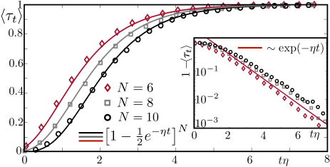
Figure 1: Purification ($\langle\tau_{t}\rangle=\langle\text{tr}\rho_{t}^{2}\rangle$) of a fully mixed initial state $\rho_{0}\sim\mathds{1}$ for strong measurements, $J=10^{-2}\eta$, and different system sizes $N$. Discrete dots are averages over $500$ simulated trajectories. Bold lines correspond to the analytical strong measurement prediction $\langle\tau_{t}\rangle=(1-\frac{1}{2}e^{-\eta t})^{N}$.

Weak measurement — The analysis of the weak measurement regime is more challenging. We consider measurement rates $\eta\ll J$ much smaller than the inverse of the time scale $\sim J^{-1}$ at which the SYK dynamics approaches ergodicity. In this case we anticipate that the information $\ln 2$ learned by measuring a single qubit is scrambled over the entire Hilbert space between two measurement events. The goal is to describe how a tiny fraction of this information is retained and a purified state reached, albeit on very large time scales. Referring to the supplemental material for more details, we represent the density operator after a sequence of $l$ projective qubit measurements as $\rho_{l}=\mathcal{N}_{l}Z_{l}$ with $\mathcal{N}_{l}=\mathrm{tr}(Z_{l})^{-1}$ and $Z_{l}=P_{l}U_{l}P_{l-1}\ldots P_{l-1}U_{l}^{\dagger}P_{l}=P_{l}U_{l}Z_{l-1}U_{l}^{\dagger}P_{l}$ in a recursive definition. Here, $P_{k}$ are projectors onto a definite state $0,1$ of any of the $N$-qubits (which one does not matter) and $U_{k}$ are $D\times D$ dimensional unitary matrices, assumed independently Haar distributed. These operators serve as proxies to the ergodic dynamics, and their independent distribution reflects the randomly distributed times between measurements. The purity after $l$ measurements is given by $\langle\mathcal{N}_{l}^{2}\mathrm{tr}(Z_{l}^{2})\rangle$. We evaluate this expression under the additional assumption of approximate statistical independence of the normalization factor and the operator trace $\langle\tau_{l}\rangle\approx\langle\mathcal{N}_{l}^{-2}\rangle^{-1}\langle\mathrm{tr}(Z_{l}^{2})\rangle$. This approximation is not backed by a small parameter and its legitimacy must be checked by comparison to exact diagonalization.

Defining $X_{2l}\equiv\langle\mathrm{tr}(Z_{l}^{2})\rangle$, and $X_{1l}\equiv\langle(\mathrm{tr}(Z_{l}))^{2}\rangle$ the recursive computation of the purity is now reduced to that of the matrix averages $X_{2l}=\langle\mathrm{tr}([P_{l}U_{l}Z_{l-1}U^{\dagger}_{l}P_{l}]^{2})\rangle$ and $X_{1l}=\langle(\mathrm{tr}(P_{l}U_{l}Z_{l-1}U^{\dagger}_{l}P_{l}))^{2}\rangle$. The Haar averaged products of four matrices can be computed in closed form (see [51]) with the simple result $X_{l}=\left(\begin{smallmatrix}z_{1}&z_{2}\cr z_{2}&z_{1}\end{smallmatrix}\right)X_{l-1}$, where $X_{l}=(X_{1l},X_{2l})^{T}$, and $z_{1}\approx 1/4$ and $z_{2}\approx 1/D$. This equation describes the evolution of the purity in terms of just two trace invariants $X_{1l,2l}$. Its structure reflects the general principle mentioned in the introduction: Chaotic mixing implies that only universal trace invariants survive at time scales exceeding the ergodicity time.

The linear recursion relation is straightforwardly solved by an exponential ansatz subject to the initial condition $X_{20}=\mathrm{tr}(\rho_{0}^{2})=D^{-1}$ and $X_{10}=(\mathrm{tr}(\rho_{0}))^{2}=1$. Noting that the step number $l=t/\eta N$ equals physical time divided by the the total measurement rate, we obtain the purity $\langle\tau_{l}\rangle=X_{2l}/X_{1l}$ as

$$\langle\tau_{t}\rangle\approx\frac{\sinh\left(\frac{t}{t_{\mathrm{p}}}\right)+D^{-1}\cosh\left(\frac{t}{t_{\mathrm{p}}}\right)}{\cosh\left(\frac{t}{t_{\mathrm{p}}}\right)+D^{-1}\sinh\left(\frac{t}{t_{\mathrm{p}}}\right)}.$$ (1)

This result predicts purification, $\langle\mathrm{tr}(\rho^{2}_{\infty})\rangle=1$, at $t\sim t_{\mathrm{p}}=D/N\eta$ no matter how small the measurement rates. However, the purification time scale, $t_{\mathrm{p}}$, now grows exponentially in the number of qubits, in contrast to the logarithmic scaling $t_{\mathrm{p}}\sim\ln(N)/\eta$ in the strong measurement regime. Figure 2 compares this prediction to numerics for $J/\eta=5\times 10^{3}$ and different system sizes, $N=6,8,10$. We indeed find data collapse for the scaled variable $t/t_{\mathrm{p}}$. For intermediate times ($\eta tN\approx D)$, Eq. (1) overestimates the purification with a maximum error of $10\%$ — likely a consequence of a partial violation of the above assumptions on statistical independence.

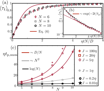
Figure 2: (a)+(b) Purification of the weakly measured system ($J=5\times 10^{3}\eta$) compared with the analytical prediction Eq.(1). The dots are obtained by averaging over $500$ numerically simulated trajectories. A scaling collapse of $\tau_{t}=\text{tr}\rho^{2}_{t}$ is obtained when evolving it in the dimensionless time $\eta tN/D$. (c) Purification time $t_{\mathrm{p},\mathrm{num}}$ (defined by $\tau_{t_{\mathrm{p},\mathrm{num}}}=0.9$) for different values of $J/\eta$. The purification time matches the weak measurement prediction (Eq. (1), red data) for $J\geq 5\eta$ and the strong measurement prediction ($t_{\mathrm{p},\mathrm{num}}\eta\sim\log(N)$, black data) for $J\leq 0.2\eta$. The scaling $t_{\mathrm{p},\mathrm{num}}\sim N^{2}$ around $J=\eta$ is associated with the vicinity of the entanglement transition, expected at $J\simeq 2\eta$ according to our theory.

The bottom panel of Fig. 2 compares the purification time $t_{\mathrm{p},\mathrm{num}}$, here defined as the time scale at which the purity has reached the value $0.9$, to the analytical predictions. It turns out that the two time dependencies $\eta t_{\mathrm{p}}\sim\ln N$ and $\eta t_{\mathrm{p}}\sim D/N$ for $\eta/J\gg 1$ and $\eta/J\ll 1$, respectively, show a remarkable degree of stability away from the limits in which they were obtained. Hinting at the existence of a phase transition, they cover almost the entire parameter axis $\eta/J$, except for a range $0.2<J/\eta<5$ where the purification time shows quadratic power law dependence $\eta t_{\mathrm{p},\mathrm{num}}\sim N^{2}$. In the following, we derive an approximate evolution equation describing the dynamics of moments of density matrices subject to a common measurement protocol. On this basis we will be able to predict the boundary between the two phases, the symmetries characterizing them, and the mechanisms safeguarding their stability.

Diagonal projection — The starting point of our construction is the observation that the random outcome of repeated measurements acts as a source of noise suppressing Fock space matrix elements $\rho_{nm}$ off-diagonal in the measurement basis, $n\not=m$, by decoherence. The stochastic Schrödinger equation formulation of measurement dynamics (see [51]) makes this interpretation concrete and can be used to derive an effective equation for the states $P\equiv\mathcal{P}\rho$, where $\mathcal{P}$ is a projector onto the subspace spanned by the Fock space diagonal states $\{|n\rangle\langle n|\}$. In the supplemental material we show that the discrete time dynamics of the diagonal coefficients $P_{n,t}$ is governed by the evolution equation

$$dP_{t}\equiv P_{t+\delta t}-P_{t}=-(\delta_{t}X_{H}+V_{\phi_{t}})P_{t},$$ (2)

where the action of the two operators on the r.h.s is defined through

$$(X_{H}P)_{n} \equiv\sum_{m}W_{nm}(P_{n}-P_{m}),$$ (3)

$$(V_{\phi}P)_{n} \equiv\sum_{i}2\phi_{i}(n_{i}-\bar{n}_{i})P_{n}.$$ (4)

Here, the first term describes incoherent transitions between different occupation states in Fock space with rates $W_{nm}=2\Gamma^{-1}|H_{nm}|^{2}$. They are induced by transient fluctuations out of the diagonal state with matrix elements $H_{nm}$, followed by relaxation back into it with a decay rate $\Gamma\sim\eta$. Specifically, for the SYK model $X_{H}=g\sum_{ijkl}(1-\sigma_{x,i}\sigma_{x,j}\sigma_{x,k}\sigma_{x,l})$, with $g=J^{2}/(\eta N^{3})$ where we used $\Gamma=\eta$, and the Pauli matrices $\sigma_{x,i}$ flip the occupation of the occupation of site $i$ according to $0,1\rightarrow 1,0$.

The second term introduces locally correlated measurement noise, $\langle\phi_{i,t}\phi_{i^{\prime},t^{\prime}}\rangle=\eta\delta t\delta_{t,t^{\prime}}\delta_{ii^{\prime}}$. The noise affects states the more the farther they are away from the instantaneous expectation values $\bar{n}_{i}\equiv\langle n_{i}\rangle=\sum_{n}P_{n}n_{i}$. (The subtraction of the expectation values also safeguards the positivity and probability conservation of the diagonal states: $d\sum_{n}P_{n}=\sum_{i}2\phi_{i}\sum_{n}P_{n}(n_{i}-\overline{n}_{i})=0$.) The self consistent coupling of the r.h.s. of Eq. (3) to the solution $P$ via the expectation values $\bar{n}_{i}$ makes the equation difficult to solve. In the following, we consider cases where these terms are expected to play no significant role. These should include the physics of the weak measurement regime, and at least qualitative aspects of the dynamics across the transition.

Generator of dynamics — Our objects of interest are $r$-fold replicated tensor products $P^{(r)}\equiv\langle P\otimes\ldots\otimes P\rangle$ averaged over noise ($r=2$ for the averaged purity). Taking the average is facilitated by the Itô-discretization of Eq. (10), i.e. $P_{t}$ depending only on the noise history at earlier times, $\{\phi_{t^{\prime}<t}\}$. Passing to a continuum description, it is then straightforward to derive the master equation [51]

$$\partial_{t}P^{(r)}=-X^{(r)}P^{(r)}$$ (5)

$$\quad X^{(r)}=\sum_{a}X^{a}_{H}-4\eta\sum_{a\not=b}n_{i}^{a}n_{i}^{b}\equiv X^{(r)}_{H}+X^{(r)}_{M},$$ (6)

where operators carrying a superscript $a$ act in the $a$th copy of the replica product space.

The generator $X^{(r)}$ describes a competition between the stochastic hopping dynamics represented by $X_{H}$, and a tendency to confine the $r$ copies of states to a common configuration of measurement outcomes $\{n_{i}\}$ (Notice the negative sign in $-4\eta$ which rewards positive correlation in replica space.) Since $X_{H}$ and $X_{M}$ appear in the effective Hamiltonian as sums over $\sim N^{4}$ and $N$ site configurations, respectively, we characterize their relative strength in terms of a parameter $\lambda\equiv(N^{4}g)/(N\eta)=N^{3}g/\eta$.

The structural similarity of Eq. (5) with an imaginary time Schrödinger equation suggests to interpret $P^{(r)}\equiv|P^{(r)}\rangle$ as a state vector with components $P^{(r)}_{n}=\langle n|P^{(r)}\rangle$, $n=(n_{1},\ldots,n_{r})$, and $X^{(r)}$ as its “effective Hamiltonian”. At large times, $|P^{(r)}_{t}\rangle\to|\Psi^{(r)}_{\lambda}\rangle$, the physical states will asymptote towards the measurement strength dependent ground states $|\Psi^{(r)}\rangle$ (the dark states of the replicated Lindbladian measurement dynamics) of $X^{(r)}$.

To understand the nature of the latter in the regimes of weak and strong measurement, respectively, it is crucial to note two discrete symmetries of $X^{(r)}$: The first is $\mathbb{Z}_{2}^{\times r}$ symmetry under $\sigma^{(a)}_{xi}\to(\pm)^{(a)}\sigma^{(a)}_{xi}$, with a replica-dependent (but $i$-independent) sign factor; this freedom represents the fermion parity symmetry of each individual of the replicated SYK systems. The second is a $\mathbb{Z}_{2}^{\times N}$ symmetry under $\sigma^{(a)}_{zi}\to(\pm)_{i}\sigma^{(a)}_{zi}$, with an $i$-dependent (but $a$-independent) sign factor; this symmetry reflects the physical equivalence of the $2^{N}$ possible measurement outcomes. In the following, we discuss how the full symmetry group $\mathbb{Z}_{2}^{\times r}\times\mathbb{Z}_{2}^{\times N}$ is broken by the ground states in the two phases of the system.

Replica symmetry breaking transition — In the limiting case of absent measurement, $\lambda\to\infty$, the effective Hamiltonian possesses the $2^{r}$-fold degenerate ground states, $|\Psi_{\infty}^{(r)}\rangle\equiv|\Psi^{(r)}_{s}\rangle=|s_{1}\rangle\otimes\ldots\otimes|s_{r}\rangle$, where $|s\rangle=|\pm\rangle\equiv\otimes_{i=1}^{n}|\pm\rangle$ with $|\pm\rangle=\frac{1}{\sqrt{2}}(|0\rangle\pm|1\rangle)$. These are cat states, fully polarized in $\pm x$-direction independently for each replica channel. Their ground state property follows from the observation that $X_{H}\equiv g(N^{4}-S^{4}_{x})$ affords a representation in terms of the global spin operator $S_{x}=\sum_{i}\sigma_{xi}$. The $2^{r}$-fold degeneracy of these states indicates that the weak measurement phase is a replica symmetry breaking phase. We also note that the ground state is uniformly distributed over Fock space, $|\langle n^{1},\ldots,n^{r}|\Psi^{(r)}_{s}\rangle|=D^{-r}$, as is typical for quantum ergodic states. Finally, the symmetry breaking is stable under the inclusion of weak but finite measurement; it takes “thermodynamically many” $\mathcal{O}(N)$ matrix elements of the measurement operator to flip one cat state into another.

In the opposite case, $\lambda=0$, we have the $2^{N}$-fold degenerate set of ground states $|\Psi^{(r)}_{n}\rangle=\bigotimes_{i}|n_{i}^{(r)}\rangle$, where $|n_{i}^{(r)}\rangle=\bigotimes_{a}|n_{i}\rangle$ are fully $\pm z$-polarized replica symmetric states, independently for each site — a “real space” symmetry breaking configuration. However, for arbitrarily weak $g>0$, only $r$ matrix elements of the operator $X_{H}$ are required to flip between states of identical replica polarization but different site configuration. The actual, non-degenerate ground state is an equal weight superposition $|\Psi^{(r)}_{0}\rangle\equiv D^{-1}\sum_{n}|\Psi^{(r)}_{n}\rangle$ showing unbroken $\mathbb{Z}_{2}^{\times r}\times\mathbb{Z}_{2}^{\times N}$symmetry: The combination of measurements and any residual system dynamics leads to an homogenization of measurement outcomes at large time scales. In the limit $J\lesssim\eta$, this homogenization can be described perturbatively in $X_{H}$ by performing a ’Schrieffer-Wolff’ transformation of the Lindbladian [51]. It also reveals the perturbative stability of the strong measurement dynamics discussed above for $0<J\lesssim\eta$.

Since the two ground states of the effective theory, $|\Psi^{(r)}_{0,\infty}\rangle$ have different symmetry, there must be a discrete symmetry breaking phase transition at a finite value of $\lambda$. An estimate for the transition threshold is obtained by comparison of the expectation values $\langle\Psi^{(r)}|X^{(r)}|\Psi^{(r)}\rangle$ in the respective states. We find that $\langle\Psi^{(r)}_{\infty}|X^{(r)}|\Psi^{(r)}_{\infty}\rangle=0$ while $\langle\Psi^{(r)}_{0}|X^{(r)}|\Psi^{(r)}_{0}\rangle=grN^{4}-4\eta r(r-1)N$, indicating a transition in the $r$-replica system at $\lambda=4(r-1)$. With $\lambda=gN^{3}/\eta=J^{2}/\eta^{2}$, and $r=2$, the energy balance suggests a transition at $J=2\eta$. This prediction is compatible with the numerically observed change in the time dependence of purification in Fig. 2.

From the ground states, one may also compute other signatures of the two phases. For example, one may introduce an entanglement cut by partition of $n=(n_{A},n_{B})$ into two bit-strings of total length $N=N_{A}+N_{B}$. Moments of the reduced (diagonal) density matrix are then obtained as $\langle\mathrm{tr}_{A}(\rho_{A}^{r})\rangle=\sum_{n_{A}}\sum_{n_{Bi}}\langle(n_{A},n_{B_{1}}),\ldots(n_{A},n_{B_{r}})|\Psi_{\lambda}\rangle$. A straightforward calculation obtains the entanglement entropies in the two phases, $S_{A}=\partial_{r}|_{r=1}\langle\mathrm{tr}_{A}(\rho_{A}^{r})\rangle$ come out as $S_{A,\lambda\gg 1}=N_{A}\ln 2$ and $S_{A,\lambda\ll 1}=0$. The change from volume law to vanishing entanglement entropy reveals $S_{A}$ as an alternative indicator of the transition [2, 1]. However, for the small system sizes considered here, this change is difficult to resolve in simulations.

Conclusions — The starting point of this paper was the observation that in the measured quantum dynamics of non-integrable systems the two sources of complexity “continued measurement” and “chaotic dynamics” to some degree neutralize each other. We exploited this principle to formulate a comprehensive approach to the description of measurement dynamics for interacting systems of mesoscopic (number of particles large but finite) extensions. Its elements included explicit calculations of the purity for strong and weak measurement, and an analysis of the symmetry breaking transition between them. In view of the growing importance of measured quantum dynamics in mesoscopic (“NISQ”) device structures, various directions of future research present themselves. For example, it would be interesting to extend the theory to systems where local correlations slow the scrambling of information by Lieb-Robinson bounds. It would also be nice to identify a one-does-it-all path integral framework, with account for coherences (required to describe the weak measurement phase), and self consistent update of measurement records (required to describe the strong measurement phase).

Appendix A Derivation of Eq. (4) in the main text

In this section, we derive Eq.(4) in the main text in a succession of two steps. We first investigate the dynamics of individual propagators $P$ for a given realization of the measurement noise, and then consider the average of multiple of these objects.

Our starting point is the observation that $P_{nmt}$ can be interpreted as the evolution of an initial density operator $\rho(0)=|m\rangle\langle m|$ to the state $\rho(t)=|n\rangle\langle n|$ by being continuously projected onto configurations diagonal in the measurement basis. To describe the evolution of this object, we consider $\rho$ as a vector in the Fock space tensor product $\mathcal{F}\otimes\mathcal{F}^{\ast}$ and introduce the projection $P=\mathcal{P}\rho$, where $(X_{\mathcal{P}})_{nm}=(\mathcal{P}X)_{nm}=\delta_{nm}X_{nn}$ projects on diagonal configurations, and $\mathcal{Q}=\mathrm{id}-\mathcal{P}$ on the complement of off-diagonal ones.

First consider the Hamiltonian contribution to the time evolution of $\rho$. Defining the “super-operator” $X_{H}\rho\equiv-i[H,\rho]$, we represent the projected von Neumann equation as

$$d_{t}\mathcal{P}\rho =\mathcal{P}X_{H}\mathcal{Q}\rho,$$ (7)

$$d_{t}\mathcal{Q}\rho =\mathcal{Q}X_{H}\mathcal{P}\rho+\mathcal{Q}X_{H}\mathcal{Q}\rho,$$ (8)

where we noted that a $\mathcal{P}X_{H}\mathcal{P}$ contribution drops out due to the commutator structure of $X_{H}$. We now solve the second equation under one phenomenological assumption (which can be backed by microscopic calculations for simple models such as the SYK model): chaotic systems efficiently decohere off-diagonal density operator matrix elements in generic bases. We thus assume that $\mathcal{Q}X_{H}\mathcal{Q}\rho\simeq-\Gamma\mathcal{Q}\rho$, with a fast decay rate, $\Gamma$, whose detailed value we leave unspecified. With this approximation, $\mathcal{Q}\rho(t)\simeq t_{\mathrm{p}}^{t}ds\,e^{-\Gamma(t-s)}\mathcal{Q}X_{H}\mathcal{P}\rho(s)\simeq\Gamma^{-1}\mathcal{Q}X_{H}\mathcal{P}\rho(t)$, and substitution into the first equation leads to $d_{t}\mathcal{P}\rho=\Gamma^{-1}(\mathcal{P}X_{H}\mathcal{Q})(\mathcal{Q}X_{H}\mathcal{P})(\mathcal{P}\rho)$. Translating back to a representation in terms of the coefficients $P_{n}$, this becomes

$$d_{t}P=-X_{H}P,\qquad(X_{H}P)_{n}=\sum_{m}W_{nm}(P_{n}-P_{m}),$$ (9)

with $W_{nm}=\frac{2}{\Gamma}|H_{nm}|^{2}$. Notice the structure of a master equation with transition rates $W_{nm}$. This structure preserves the positivity and probability conservation of the distribution $P$.

In contrast to the Hamiltonian, the measurement operator stays within the diagonal subspace defined by the measurement basis. Its action can be inferred from the discrete time stochastic Schrödinger equation, $d|\psi_{t}\rangle\equiv|\psi_{t+\delta t}\rangle-|\psi_{t}\rangle=(-i\delta tH-\frac{\eta\delta t}{2}\sum_{i}M_{i}^{2}+\sum_{i}\phi_{i}M_{i})|\psi_{t}\rangle$, where the measurement noise is Gaussian correlated with $\langle\phi_{i,t}\phi_{i^{\prime},t^{\prime}}\rangle=\delta t\eta\delta_{t,t^{\prime}}\delta_{ii^{\prime}}$, the operator $M_{i}=O_{i}-\bar{O}_{i}$ contains the measurement operator self consistently corrected for the instantaneous average $\bar{O}_{i}=\langle\psi|O_{i}|\psi\rangle=\sum_{n}O_{i,n}P_{n}$. A Taylor expansion of the discrete evolution equation of $\rho_{t}=|\psi_{t}\rangle\langle\psi_{t}|$ to leading order in $\delta t$ (including the standard replacement $\phi_{i,t}\phi_{i^{\prime},t}\to\delta t\eta\delta_{ii^{\prime}}$) then defines the measurement contribution to the evolution as

$$-V_{\phi}P =\sum_{i}\left(\frac{\eta\delta t}{2}(\{M_{i}^{2},P\}-2M_{i}PM_{i})+\{\phi_{i}M_{i},P\}\right)$$

$$=2\sum_{i}\delta\phi_{i}M_{i}P.$$

Adding the Hamiltonian contribution, we obtain the discrete time evolution equation

$$dP_{t}\equiv P_{t+\delta t}-P_{t}=-(\delta tX_{H}+V_{\phi_{t}})P_{t},$$ (10)

where $P_{n0}=\delta_{n,m}$. What makes this equation complicated (nonlinear) is the self consistent dependence of $V_{\phi}$ on the r.h.s. on the solution via the averages $\bar{O}_{i}$. However, in the regimes studied in this paper, these values either average out (strong measurement phase), or are intrinsically small (weak measurement phase). We therefore ignore them throughout, and replace $M_{i}\to O_{i}$ by the naked measurement operators.

We now consider the noise average of the “tensor product” $P^{(r)}=\langle P\otimes\ldots\otimes P\rangle$ of $r$ propagators. (It is useful to think about these expressions in a quantum mechanics inspired language: in it, individual $P$’s represent time dependent “wave functions” $P_{n}(t)=P_{nt}$ with initial values $P_{n0}=\delta_{nm}$, and the above is their $r$-body generalization.) To obtain Eq. (5) in the main text, we consider the time differences $dP^{(r)}_{t}=\langle\bigotimes P_{t+dt}-\bigotimes P_{t}\rangle$, and expand to up to second order in $d_{t}$. The first order expansion leads to $-\delta t\sum_{a}X_{H}^{a}P^{(r)}_{t}$ the first term in Eq. (4) in the main text, and the second order one to a an operator $4\sum_{a\not=b}\sum_{ij}\langle\phi_{i,t}\phi_{j,t}\rangle O_{i}^{a}O_{j}^{b}\,P^{(r)}_{t}$, where we used that $P_{t}$ depends only on $\{\phi_{t^{\prime}<t}\}$ and so the average over $\phi_{t}$ decouples. From the Gaussian correlation of $\phi_{i,t}$ we obtain $4\delta t\eta\sum_{a\not=b}\sum_{i}O^{a}_{i}O^{b}_{i}P^{(r)}_{t}$. Adding the Hamiltonian operator dividing by $\delta$ and taking the continuum limit, we obtain Eq. (4).

Appendix B Weak measurement

In this section, we discuss in detail how the average purification is obtained for the protocol of sporadic projective measurements described in the main text. An initial maximally mixed configuration, $\rho_{0}=\frac{1}{D}\mathds{1}$ remains invariant under system evolution, until the first measurement of qubit no. $i$ in state $n_{i}$. After it, the density operator is given by $\frac{2}{D}P_{1}$, where $P_{1}\equiv P_{i}^{n_{i}}$ projects the $i$th qubit onto a state $n$, and time evolution under $U_{\Delta t}\equiv U$ up to a time $\Delta t$ defines the state $\rho_{1}\equiv\mathcal{N}_{1}U_{1}P_{1}U_{1}^{\dagger}$, with normalization $\mathcal{N}_{1}^{-1}=\mathrm{tr}(U_{1}P_{1}U_{1}^{\dagger})=D/2$. A second projective measurement, now of qubit $j$, collapses this state to $\rho_{2}\equiv\mathcal{N}_{2}P_{2}U_{1}P_{1}U_{1}^{\dagger}P_{2}$, with a second projector $P_{2}\equiv P_{j}^{n_{j}}$, and updated normalization $\mathcal{N}_{2}^{-1}=\mathrm{tr}(P_{2}U_{1}P_{1}U_{1}^{\dagger}P_{2})$.

Iteration of this evolution defines the state $\rho_{l}=\mathcal{N}_{l}Z_{l}$ with $\mathcal{N}_{l}=\mathrm{tr}(Z_{l})$ and $Z_{l}=P_{l}U_{l}P_{l-1}\ldots P_{l-1}U_{l}^{\dagger}P_{l}$, or $Z_{l}=P_{l}U_{l}Z_{l-1}U_{l}^{\dagger}P_{l}$ in a recursive definition. The purity after $l$ measurements is given by $\langle\mathcal{N}_{l}^{2}\mathrm{tr}(Z_{l}^{2})\rangle$. We evaluate this expression under the simplifying assumptions mentioned in the main text: statistical independence of different $U_{k}$, and independence of the normalization factor and the operator trace $\langle\tau\rangle\approx\langle\mathcal{N}_{l}^{-2}\rangle^{-1}\langle\mathrm{tr}(Z_{l}^{2})\rangle$.

The statistics of each update step then reduces to the computation of Haar averages of four matrix elements of $U$ and its adjoint. For a generic set of matrix elements, we have the formula (from now on, $\langle\ldots\rangle$ denotes Haar measure averaging)

$$\langle U^{\vphantom{\dagger}}_{kl}U^{\vphantom{\dagger}}_{mn}U^{\dagger}_{n^{\prime}m^{\prime}}U^{\dagger}_{l^{\prime}k^{\prime}}\rangle=$$ (11)

$$\quad=c_{1}\delta_{kk^{\prime}}\delta_{ll^{\prime}}\delta_{mm^{\prime}}\delta_{nn^{\prime}}+c_{1}\delta_{km^{\prime}}\delta_{ln^{\prime}}\delta_{mk^{\prime}}\delta_{nl^{\prime}}+$$ (12)

$$\quad+c_{2}\delta_{kk^{\prime}}\delta_{ln^{\prime}}\delta_{mm^{\prime}}\delta_{nl^{\prime}}+c_{2}\delta_{km^{\prime}}\delta_{ll^{\prime}}\delta_{mk^{\prime}}\delta_{nn^{\prime}},$$ (13)

with coefficients $c_{1}=(D^{2}-1)^{-1}$ and $c_{2}=-(D(D^{2}-1))^{-1}$.

Recursion: From this general fourth moment it is straightforward to compute the trace averages

$$\langle\mathrm{tr}(BUAU^{\dagger}BUAU^{\dagger})\rangle=$$ (14)

$$\quad=\frac{1}{D^{2}-1}\Big{(}\mathrm{tr}(B^{2})(\mathrm{tr}(A))^{2}+(\mathrm{tr}(B))^{2}\mathrm{tr}(A^{2})-$$ (15)

$$\quad-\frac{1}{D}\mathrm{tr}(A^{2})\mathrm{tr}(B^{2})-\frac{1}{D}(\mathrm{tr}(A)\mathrm{tr}(B))^{2}\Big{)}$$ (16)

$$\langle(\mathrm{tr}(BUAU^{\dagger}))^{2}\rangle=$$ (17)

$$=\frac{1}{D^{2}-1}\Big{(}(\mathrm{tr}(A))^{2}(\mathrm{tr}(B))^{2}+\mathrm{tr}(A^{2})\mathrm{tr}(B^{2})-$$ (18)

$$\quad-\frac{1}{D}(\mathrm{tr}(A))^{2}\mathrm{tr}(B^{2})-\frac{1}{D}(\mathrm{tr}(B))^{2}\mathrm{tr}(A^{2})\Big{)}$$ (19)

for general matrix operators $A,B$. We now use these expressions to the one measurement step purity update. To this end, define the two traces $X^{\prime}_{1}=\langle(\mathrm{tr}(Z^{\prime}))^{2}\rangle$ and $X^{\prime}_{2}=\langle\mathrm{tr}(Z^{\prime 2})\rangle$ with $Z^{\prime}\equiv Z_{l-1}$. We now consider the update relation $Z\equiv Z_{l}=PUZ^{\prime}U^{\dagger}P$ with $U\equiv U_{l}$, $P\equiv P_{l}$ and the updated traces $X_{1}=\langle(\mathrm{tr}(Z))^{2}\rangle=\langle(\mathrm{tr}(PUZ^{\prime}U^{\dagger}P))^{2}\rangle$ and $X_{2}=\langle\mathrm{tr}(PUZ^{\prime}U^{\dagger}PUZ^{\prime}U^{\dagger})\rangle$. The structure of these traces is covered by the above auxiliary relations. With $\mathrm{tr}(P)=D/2$, a straightforward computation leads to the closed relation

$$X=\left(\begin{matrix}z_{1}&z_{2}\cr z_{2}&x_{1}\end{matrix}\right)X^{\prime},$$ (20)

where $X=(X_{1},X_{2})^{T}$, and $z_{1}=\frac{D}{2}(\frac{D}{2}c_{1}+c_{2})$, $z_{2}=\frac{D}{2}(\frac{D}{2}c_{2}+c_{1})$. With the matrix eigenvectors $|\pm\rangle$, eigenvalues $(z_{1}\pm z_{2})$, the initial condition $X_{0}=(1,D^{-1})$ describing a normalized and fully mixed state, and the overlap $\langle\pm|X_{0}\rangle=\frac{1}{\sqrt{2}}(1+sD^{-1})$, the recursion relation is solved by

$$X_{l}=\frac{1}{\sqrt{2}}\sum_{s=\pm}|s\rangle(z_{1}+sz_{2})^{l}(1+sD^{-1}).$$ (21)

From here, we obtain the purity of the normalized states as $\langle\tau_{l}\rangle=X_{2l}/X_{1l}$ as

$$\langle\tau_{l}\rangle\approx\frac{(z_{1}+z_{2})^{l}(1+D^{-1})-(z_{1}-z_{2})^{l}(1-D^{-1})}{(z_{1}+z_{2})^{l}(1+D^{-1})+(z_{1}-z_{2})^{l}(1-D^{-1})}$$ (22)

To leading order in an expansion in $D^{-1}$, we have $z_{1}\pm z_{2}\approx\frac{1}{4}\pm\frac{1}{D}$. In this approximation, and for large $l\sim t/\eta N\gg 1$ the above expression then simplifies to Eq. (1) of the main text.

Appendix C Stability of the two phases

In this section, we discuss the stability of the weak and the strong measurement regimes away from the limits of diverging and vanishing strength parameters, respectively.

Weak measurement — Evidence for the stability of the weak measurement regime follows from the analysis of the purification time in the main text. The essential condition leading to a $J$-independent time scale $t_{\mathrm{p}}\sim D/N\eta$ was $J>N\eta$, i.e. full scrambling at time scales shorter than the time between two measurements. The numerical analysis indeed confirms the presence of an extended regime of $J$-independent $t_{\mathrm{p}}$. This is illustrated in Fig. 3, where purification trajectories for $J\gg\eta$ (in particular $J\geq 20\eta$ for $N=8$ qubits) quickly converge onto a $J$-independent evolution, and corresponding to the limit $J\rightarrow\infty$. In the language of the generator $X^{(r)}$ the same phenomenon is expressed through the stability of the cat ground states $|\Psi^{(r)}_{\infty}\rangle$. Besides the exponentially long purification time, this state is characterized by a volume law entanglement entropy, $S_{a}=N_{A}\ln 2$, where $N_{A}$ is the bipartition size.

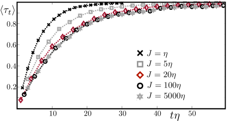
Figure 3: Purity $\langle\tau_{t}\rangle=\langle\text{tr}\rho_{t}^{2}\rangle$ as a function of time of an initially fully mixed state $\rho_{0}\sim\mathds{1}$ for $N=8$ qubits and for different values of $J/\eta$. For $J\gg\eta$ the purification dynamics becomes $J$-independent and the curves for larger and larger $J$ converge towards the curve describing the $J=\infty$ limit. In this limit, the evolution is independent of the value of $J$ as predicted by an evolution with independent, Haar-random matrices.

Strong measurement — In the regime of strong measurement, the dominant generator $X_{M}^{(r)}$ requires fast relaxation into any one of the replica homogeneous states $|\Psi_{n}^{(r)}\rangle$ defined in the main text. Physically, these are states of identical measurement result, $n$, in each replica channel. To understand what happens within the $2^{N}$-fold degenerate space of these states, we perturbatively include the operator $X_{H}^{(r)}$ into the picture. More specifically, one may employ a Schrieffer-Wolff transformation to derive an operator describing virtual transitions out of the measurement ground state induced by $X_{H}^{(r)}$. For example, for two replicas, $r=2$, this operator reads $X_{\mathrm{SW}}^{(2)}=c\frac{g^{2}}{\eta}\sum_{ijkl}(\sigma_{xi}^{1}\otimes\sigma_{xi}^{2})\ldots(\sigma_{xl}^{1}\otimes\sigma_{xl}^{2})$, with a numerical constant $c$. This operator mixes between different $|\Psi_{n}^{(2)}\rangle$. Its ground state is the uniform superposition $|\Psi_{0}^{(2)}\rangle=\frac{1}{D}\sum_{n}|\Psi_{n}^{(2)}\rangle$ mentioned in the main text. As long as we are in the regime of perturbative stability of this construction, $J\lesssim\eta$ this replica symmetric configuration should describe the state of the system. Salient features of the construction include fast purification time, $t_{\mathrm{d}}\simeq\eta^{-1}\ln N$ and vanishing entanglement entropy.

Appendix D Numerical implementation

In order to simulate the purification dynamics numerically, we implement the monitored Lindblad evolution for the complete density matrix $\rho_{t}$. In each time step, the density matrix evolves under the stochastic master equation $(d\rho_{t}=\rho_{t+\delta t}-\rho_{t})$

$$d\rho_{t} =-i\delta t[H,\rho_{t}]-\sum_{i}\frac{\eta\delta t}{2}[M_{i},[M_{i},\rho]]+\{\phi_{i}M_{i},\rho_{t}\}.$$

Here, $H$ is the SYK Hamiltonian and $M_{i}=n_{i}-\text{tr}(\rho_{t}n_{i})$ are the measurement operators as provided in the main text. Due to the Itô calculus, $\phi_{i}\phi_{j}=\eta\delta t\delta_{i,j}$, each time step is efficiently implemented by a Trotterized protocol, consisting of a matrix multiplication $\rho_{t+\delta t}=V_{t}U\rho_{t}U^{\dagger}V_{t}$ with $V_{t}=\exp(-\sum_{i}\eta\delta tM_{i}^{2}-\phi_{i}M_{i})$ and $U=\exp(-iH\delta t)$. The matrix $V_{t}$ has to be computed in each time step due to the dependence of the operators $M_{i}$ on $\rho_{t}$. The computation of $V_{t}$ and the multiplication with $\rho_{t}$ can be implemented efficiently since $V_{t}$ is diagonal in the local Fock state basis. The off-diagonal matrix $U$ is time independent and is computed only once per trajectory from the SYK Hamiltonian $H$.

In the simulations, we work in units of $\eta=1$, a time discretization of $\delta t=0.05$ and perform averages over $500$ simulated trajectories for each set of parameters. We have tested also smaller time discretizations down to $\delta t=0.001$ for limiting cases of small and large $J$ but no qualitative differences have been observed. For each trajectory, one realization of the SYK Hamiltonian is determined by randomly drawing the couplings $J_{abcd}$ from a Gaussian distribution with zero mean and variance $\langle J_{abcd}^{2}\rangle=6J^{2}/(2N)^{3}$. The trajectory average therefore represents both an average over different measurement outcomes and over SYK realizations. For $N=8$ and $N=10$ we also simulated a limited number of trajectories corresponding to the same SYK Hamiltonian, and we have not observed any significant difference compared to drawing a new Hamiltonian for each trajectory.

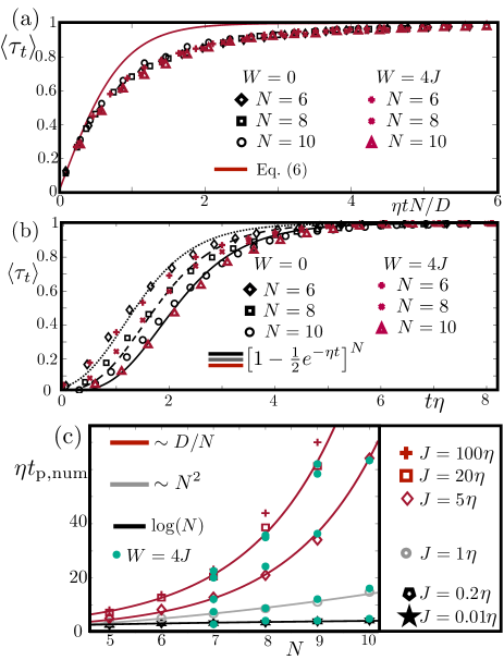
Figure 4: Purification with additional two-body hopping Hamiltonian $\hat{H}_{2}$ with a bandwidth $W=4J$. (a) Time evolution of the purity $\langle\tau_{t}\rangle=\langle\text{tr}\rho_{t}^{2}\rangle$ for an initial maximally mixed state $\rho_{0}\sim\mathds{1}$ at weak measurement rate ($J=5\times 10^{3}\eta$) for different system sizes $N$. We compare the purification without two-body Hamiltonian, $W=0$ (black symbols), to the purification with two-body Hamiltonian, $W=4J$ (red symbols). Both cases collapse onto the same trajectory after appropriate rescaling of time by the Hilbert space dimension $D$. The $W=0$ data is identical to Fig. 2 (a) in the main text. (b) Same comparison as in (a) but for strong measurement rate ($J=10^{-2}\eta$). The data for $W=0$ and $W=4$ both match the analytical prediction for $J=0$. (c) Numerically obtained purification times $t_{\text{p,num}}$ for $W=4$ (turquoise) on top of the $W=0$ data from Fig. 2(c) in the main text. No change in the general behavior or on the location of the purification transition is observed (see Fig. 2 in the main text for more details).

Appendix E Purification with additional two-body Hamiltonian

In order to verify the robustness of the purification dynamics against perturbations, we consider an additional two-body Hamiltonian, such that $\hat{H}=\hat{H}_{2}+\hat{H}_{\text{int}}$, were $\hat{H}_{\text{int}}$ is the four-body SYK Hamiltonian analyzed in the main text. For $\hat{H}_{2}$ we assume a nearest neighbor hopping Hamiltonian, which is off-diagonal in the measurement basis and has a bandwidth $W$. For concreteness, it is given by $\hat{H}_{2}=\frac{W}{4}\sum_{l}(c^{\dagger}_{l}c_{l+1}+\text{H.c.})$. In the main text, we examined the behavior for $W=0$, where the ground state of the system is a non-Fermi liquid. Here, we look at the case $W>J$ to verify that in the opposite Fermi liquid regime, too, the system undergoes a purification transition with the same properties.

We test this limit by numerical simulation of the purification dynamics at a fixed bandwidth $W=4J$. The results are shown in Fig. 4, where we compare the time evolution for weak measurements Fig. 4(a), strong measurements (b) and the purification times (c) for the cases $W=0$ and $W=4J$. As seen in the figure, there are no detectable differences in the purification trajectories nor in the purification times in both cases. This leads to the conclusion that the purification is dominated exclusively by the non-integrable part of the Hamiltonian $\hat{H}_{\text{int}}$.

References

- Skinner et al. [2019] B. Skinner, J. Ruhman, and A. Nahum, Measurement-induced phase transitions in the dynamics of entanglement, Phys. Rev. X 9, 031009 (2019).
- Li et al. [2018] Y. Li, X. Chen, and M. P. A. Fisher, Quantum zeno effect and the many-body entanglement transition, Phys. Rev. B 98, 205136 (2018).
- Li et al. [2019] Y. Li, X. Chen, and M. P. A. Fisher, Measurement-driven entanglement transition in hybrid quantum circuits, Phys. Rev. B 100, 134306 (2019).
- Gullans and Huse [2020a] M. J. Gullans and D. A. Huse, Dynamical purification phase transition induced by quantum measurements, Phys. Rev. X 10, 041020 (2020a).
- Choi et al. [2020] S. Choi, Y. Bao, X.-L. Qi, and E. Altman, Quantum error correction in scrambling dynamics and measurement-induced phase transition, Phys. Rev. Lett. 125, 030505 (2020).
- Fan et al. [2021] R. Fan, S. Vijay, A. Vishwanath, and Y.-Z. You, Self-organized error correction in random unitary circuits with measurement, Phys. Rev. B 103, 174309 (2021).
- Nahum et al. [2021] A. Nahum, S. Roy, B. Skinner, and J. Ruhman, Measurement and entanglement phase transitions in all-to-all quantum circuits, on quantum trees, and in landau-ginsburg theory, PRX Quantum 2, 010352 (2021).
- Lavasani et al. [2021] A. Lavasani, Y. Alavirad, and M. Barkeshli, Measurement-induced topological entanglement transitions in symmetric random quantum circuits, Nature Physics 17, 342–347 (2021).
- Doggen et al. [2021] E. V. H. Doggen, Y. Gefen, I. V. Gornyi, A. D. Mirlin, and D. G. Polyakov, Generalized quantum measurements with matrix product states: Entanglement phase transition and clusterization (2021), arXiv:2104.10451 .
- Bao et al. [2021] Y. Bao, S. Choi, and E. Altman, Symmetry enriched phases of quantum circuits, Annals of Physics , 168618 (2021).
- Jian et al. [2021a] S.-K. Jian, C. Liu, X. Chen, B. Swingle, and P. Zhang, Quantum error as an emergent magnetic field (2021a), arXiv:2106.09635 .
- Turkeshi et al. [2021] X. Turkeshi, A. Biella, R. Fazio, M. Dalmonte, and M. Schiró, Measurement-induced entanglement transitions in the quantum ising chain: From infinite to zero clicks, Phys. Rev. B 103, 224210 (2021).
- Ippoliti et al. [2021] M. Ippoliti, M. J. Gullans, S. Gopalakrishnan, D. A. Huse, and V. Khemani, Entanglement phase transitions in measurement-only dynamics, Phys. Rev. X 11, 011030 (2021).
- Zabalo et al. [2020] A. Zabalo, M. J. Gullans, J. H. Wilson, S. Gopalakrishnan, D. A. Huse, and J. H. Pixley, Critical properties of the measurement-induced transition in random quantum circuits, Phys. Rev. B 101, 060301 (2020).
- Zabalo et al. [2022] A. Zabalo, M. J. Gullans, J. H. Wilson, R. Vasseur, A. W. W. Ludwig, S. Gopalakrishnan, D. A. Huse, and J. H. Pixley, Operator Scaling Dimensions and Multifractality at Measurement-Induced Transitions, Phys. Rev. Lett. 128, 050602 (2022).
- Li and Fisher [2021] Y. Li and M. P. A. Fisher, Statistical mechanics of quantum error correcting codes, Phys. Rev. B 103, 104306 (2021).
- Jian et al. [2020a] C.-M. Jian, Y.-Z. You, R. Vasseur, and A. W. W. Ludwig, Measurement-induced criticality in random quantum circuits, Phys. Rev. B 101, 104302 (2020a).
- Jian et al. [2021b] S.-K. Jian, C. Liu, X. Chen, B. Swingle, and P. Zhang, Measurement-induced phase transition in the monitored sachdev-ye-kitaev model, Phys. Rev. Lett. 127, 140601 (2021b).
- Buchhold et al. [2021] M. Buchhold, Y. Minoguchi, A. Altland, and S. Diehl, Effective theory for the measurement-induced phase transition of dirac fermions, Phys. Rev. X 11, 041004 (2021).
- Alberton et al. [2021] O. Alberton, M. Buchhold, and S. Diehl, Entanglement transition in a monitored free-fermion chain: From extended criticality to area law, Phys. Rev. Lett. 126, 170602 (2021).
- Minato et al. [2022] T. Minato, K. Sugimoto, T. Kuwahara, and K. Saito, Fate of Measurement-Induced Phase Transition in Long-Range Interactions, Phys. Rev. Lett. 128, 010603 (2022).
- Block et al. [2022] M. Block, Y. Bao, S. Choi, E. Altman, and N. Y. Yao, Measurement-Induced Transition in Long-Range Interacting Quantum Circuits, Phys. Rev. Lett. 128, 010604 (2022).
- Müller et al. [2022] T. Müller, S. Diehl, and M. Buchhold, Measurement-Induced Dark State Phase Transitions in Long-Ranged Fermion Systems, Phys. Rev. Lett. 128, 010605 (2022).
- Biella and Schiró [2021] A. Biella and M. Schiró, Many-body quantum zeno effect and measurement-induced subradiance transition, Quantum 5, 528 (2021).
- Szyniszewski et al. [2020] M. Szyniszewski, A. Romito, and H. Schomerus, Universality of entanglement transitions from stroboscopic to continuous measurements, Physical Review Letters 125, 10.1103/physrevlett.125.210602 (2020).
- Szyniszewski et al. [2019] M. Szyniszewski, A. Romito, and H. Schomerus, Entanglement transition from variable-strength weak measurements, Phys. Rev. B 100, 064204 (2019).
- Fuji and Ashida [2020] Y. Fuji and Y. Ashida, Measurement-induced quantum criticality under continuous monitoring, Phys. Rev. B 102, 054302 (2020).
- Boorman et al. [2022] T. Boorman, M. Szyniszewski, H. Schomerus, and A. Romito, Diagnostics of entanglement dynamics in noisy and disordered spin chains via the measurement-induced steady-state entanglement transition, Phys. Rev. B 105, 144202 (2022).
- Lunt and Pal [2020] O. Lunt and A. Pal, Measurement-induced entanglement transitions in many-body localized systems, Phys. Rev. Research 2, 043072 (2020).
- Sang et al. [2021a] S. Sang, Y. Li, T. Zhou, X. Chen, T. H. Hsieh, and M. P. Fisher, Entanglement negativity at measurement-induced criticality, PRX Quantum 2, 10.1103/prxquantum.2.030313 (2021a).
- Ippoliti and Khemani [2021] M. Ippoliti and V. Khemani, Postselection-free entanglement dynamics via spacetime duality, Physical Review Letters 126, 10.1103/physrevlett.126.060501 (2021).
- Nahum and Skinner [2020] A. Nahum and B. Skinner, Entanglement and dynamics of diffusion-annihilation processes with majorana defects, Phys. Rev. Research 2, 023288 (2020).
- Gullans and Huse [2020b] M. J. Gullans and D. A. Huse, Scalable probes of measurement-induced criticality, Phys. Rev. Lett. 125, 070606 (2020b).
- Noel et al. [2021] C. Noel, P. Niroula, D. Zhu, A. Risinger, L. Egan, D. Biswas, M. Cetina, A. V. Gorshkov, M. J. Gullans, D. A. Huse, and C. Monroe, Observation of measurement-induced quantum phases in a trapped-ion quantum computer (2021), arXiv:2106.05881 .
- Sang and Hsieh [2021] S. Sang and T. H. Hsieh, Measurement-protected quantum phases, Physical Review Research 3, 10.1103/physrevresearch.3.023200 (2021).
- Sang et al. [2021b] S. Sang, Y. Li, T. Zhou, X. Chen, T. H. Hsieh, and M. P. Fisher, Entanglement negativity at measurement-induced criticality, PRX Quantum 2, 10.1103/prxquantum.2.030313 (2021b).
- Chen et al. [2020] X. Chen, Y. Li, M. P. A. Fisher, and A. Lucas, Emergent conformal symmetry in nonunitary random dynamics of free fermions, Phys. Rev. Research 2, 033017 (2020).
- Li et al. [2021a] Y. Li, X. Chen, A. W. W. Ludwig, and M. P. A. Fisher, Conformal invariance and quantum nonlocality in critical hybrid circuits, Physical Review B 104, 10.1103/physrevb.104.104305 (2021a).
- Zhang et al. [2021] P. Zhang, S.-K. Jian, C. Liu, and X. Chen, Emergent replica conformal symmetry in non-hermitian syk2 chains, Quantum 5, 579 (2021).
- Jian et al. [2020b] C.-M. Jian, B. Bauer, A. Keselman, and A. W. W. Ludwig, Criticality and entanglement in non-unitary quantum circuits and tensor networks of non-interacting fermions (2020b), arXiv:2012.04666 .
- Li et al. [2021b] Y. Li, R. Vasseur, M. P. A. Fisher, and A. W. W. Ludwig, Statistical mechanics model for clifford random tensor networks and monitored quantum circuits (2021b), arXiv:2110.02988 .
- Bao et al. [2020] Y. Bao, S. Choi, and E. Altman, Theory of the phase transition in random unitary circuits with measurements, Phys. Rev. B 101, 104301 (2020).
- Cao et al. [2019] X. Cao, A. Tilloy, and A. D. Luca, Entanglement in a fermion chain under continuous monitoring, SciPost Phys. 7, 24 (2019).
- Minoguchi et al. [2022] Y. Minoguchi, P. Rabl, and M. Buchhold, Continuous gaussian measurements of the free boson CFT: A model for exactly solvable and detectable measurement-induced dynamics, SciPost Physics 12 (2022).
- Caves and Milburn [1987] C. M. Caves and G. J. Milburn, Quantum-mechanical model for continuous position measurements, Phys. Rev. A 36, 5543 (1987).
- Snizhko et al. [2021] K. Snizhko, P. Kumar, N. Rao, and Y. Gefen, Weak-measurement-induced asymmetric dephasing: Manifestation of intrinsic measurement chirality, Physical Review Letters 127, 10.1103/physrevlett.127.170401 (2021).
- Bentsen et al. [2021] G. S. Bentsen, S. Sahu, and B. Swingle, Measurement-induced purification in large-n hybrid brownian circuits, Physical Review B 104, 10.1103/physrevb.104.094304 (2021).
- Gopalakrishnan and Gullans [2021] S. Gopalakrishnan and M. J. Gullans, Entanglement and purification transitions in non-hermitian quantum mechanics, Physical Review Letters 126, 10.1103/physrevlett.126.170503 (2021).
- Kurland et al. [2000] I. L. Kurland, I. L. Aleiner, and B. L. Altshuler, Mesoscopic magnetization fluctuations for metallic grains close to the stoner instability, Phys. Rev. B 62, 14886 (2000).
- Altland et al. [2019] A. Altland, D. Bagrets, and A. Kamenev, Sachdev-ye-kitaev non-fermi-liquid correlations in nanoscopic quantum transport, Phys. Rev. Lett. 123, 226801 (2019).
- [51] See supplementary material appended to this manuscript for the detailed derivation of Eq.(5) and a discussion about the perturbative stability of the strong and weak measurement regimes.