Estimating Uncertainty For Vehicle Motion Prediction on Yandex Shifts Dataset

Abstract

Motion prediction of surrounding agents is an important task in context of autonomous driving since it is closely related to driver’s safety. Vehicle Motion Prediction (VMP) track of Shifts Challenge focuses on developing models which are robust to distributional shift and able to measure uncertainty of their predictions. In this work we present the approach that significantly improved provided benchmark and took 2nd place on the leaderboard.

1 Introduction

The task of multimodal trajectory prediction of road agents was thoroughly analyzed during past years and has led to the emergence of several groups of methods. One common approach is to use Computer Vision (CV) models with rasterized scene images as inputs [1], [2]. However, powerful CV models have a large number of parameters, could be computationally intensive and quite slow on inference. The disadvantages also include encoding a quite large amount of irrelevant to the underlying process information from the entire scene. To overcome these drawbacks most state-of-the-art approaches lean on the graph structure [3], [4]. Graph-based methods take into account only relevant to the driving patterns information and can provide better quality due to the expressive power of graph neural networks [5], [6]. Several approaches further improve the results by increasing the complexity of trajectory decoders [7], [8].

However, the problem of uncertainty estimation (UE) in the context of VMP has not been widely covered yet. Previous works [9], [10], [11] consider a limited number of methods and are either disconnected from state-of-the-art approaches in VMP or recent advances in UE field [12], [13], [14] or both. On the other hand, Bayesian Deep Learning field would benefit from benchmarking on large industrial datasets.

In this work we constructed and benchmarked the solution that simultaneously tries to meet the needs of VMP task and uses recent advances in both VMP and UE fields. In what follows, we describe the dataset and our solution.

2 Approach

In our work we adopt a single forward pass method for uncertainty estimation. The resulting model has two parts: multimodal motion prediction component and external neural network [15] to model the uncertainty. The general setting is shown on the Figure 1. Both components use graph representation of the scene which we describe in the following section and process them with graph neural networks (GNN).

2.1 Problem Statement

The Vehicle Motion prediction part of Shifts Dataset [16] contains 5 seconds of past and 5 seconds of future states for all agents in a scene along with overall scene features. The goal of the challenge is to build a model that predicts $k\leq 5$ future trajectories $\tilde{y}_{i}^{k}$ in the horizon of $T=25$ timesteps along with their confidences $\omega^{k}$ and overall scene uncertainty $U$ for each scene $\mathbf{x}_{i}$.

The dataset $\mathcal{D}=\{(\mathbf{x}_{i},\mathbf{y}_{i})\}_{i=1}^{N}$, where $\mathbf{x}_{i}$ are features of the scenes, $\mathbf{y}_{i}\in\mathbb{R}^{T\times 2}$ are ground truth trajectories and $i$ is the scene index, is divided into 3 parts: train part contains only scenes from Moscow with no precipitation, but there are different locations and precipitations in development and evaluation parts in order to create data shift setting.

2.2 Data Preprocessing

We extract geometries for parts of the road lanes and crosswalk polygons from provided raw data and use past observed trajectories of all agents in the scene as is. We refer to these elementary geometries as polylines following [3].

Following this, we transform coordinates so that the origin is located at the target agent’s last observed position, and the vehicle is headed towards positive direction of x-axis. We select points within squared bounding box of size $120$ meters centered at the origin in order to capture only relevant information. After that we redistribute points of lane and crosswalk geometries to impose the constant distance of $d=2$ meters between adjacent points. Finally, we create fully-connected subgraphs for each polyline and invert them. In the end of all operations the whole scene is represented as a graph with fully-connected components which correspond to polylines. An example of the processed scene is shown on the Figure 1.

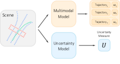
(a)

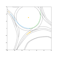
(b)

Figure 1: (left) Structure of the composite model. (right) An example of the preprocessed scene. Black points represent lanes, blue and green - past and future target agent’s trajectories respectively, orange depicts other agents in the scene.

We construct the node feature-matrix of the form $X_{i}=(p_{i}^{s},p_{i}^{e},f_{i})$, where $p_{i}^{s}\in\mathbb{R}^{2}$, $p_{i}^{e}\in\mathbb{R}^{2}$ are the coordinates of "start" and "end" adjacent points which formed a node after inversion, $f_{i}\in\mathbb{R}^{9}$ are feature-vectors which we fill differently for various polyline types and $i$ is the node index. Namely, we use maxspeed, lane priority and lane availability for lane polylines. Lane availability status takes into account the traffic light state only at the latest available timestamp. For agent polylines we fill in the following ones: timestamp, vectors of velocity and acceleration, yaw. It is worth mentioning that in contrast to [3] we do not use integer ids of polylines as features.

2.3 Multimodal Model

We adopt VectorNet [3] architecture to obtain a hidden representation for each scene. VectorNet is an hierarchical graph neural network that firstly builds vector representations for each polyline subgraph and then propagates signal among all obtained representations. The model is trained using corrected NLL of gaussian mixture as loss function: $\mathcal{L}=-\log\sum_{k}\omega^{k}\prod_{t=1}^{T}\mathcal{N}(y_{t}|\tilde{y}_{t}^{k},I)-T\log(2\pi)$.

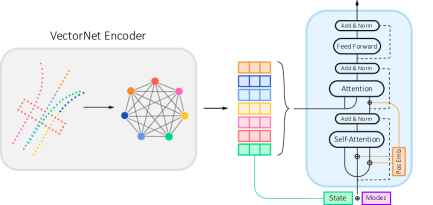
Figure 2: VectorNet-based Transformer.

At the first stage we obtain embeddings for each node of fully connected subgraphs by applying Message Passing [17]:

$$h^{(t)}_{i}=\mathcal{U}^{(t)}\left(h^{(t-1)}_{i},\Box_{j\in\mathcal{N}(i)}\mathcal{M}^{(t)}(h^{(t-1)}_{i},h^{(t-1)}_{j})\right),$$ (1)

where $h_{i}^{(t)}$ - representation of node with index $i$ at layer $t$, $\mathcal{N}(i)$ - neighbourhood of node $i$, which is formed by all other nodes in polyline in our case, $\Box$ - aggregation function, $\mathcal{U}$ and $\mathcal{M}$ - update and message functions respectively. We use $\max$ as aggregation function, MLP as message and concatenation as update. After that we apply maxpooling on top of node embeddings in order to get vector representation $d_{k}$ for the whole polyline with index $k$.

At the second stage we construct fully-connected graph from all polyline representations $d$ and apply graph transformer convolution [18]:

$$d^{(t)}_{k}=W_{1}d^{(t-1)}_{k}+\sum_{l\in\mathcal{N}(k)}\alpha_{kl}W_{2}d^{(t-1)}_{l},\quad\alpha_{kl}=\textrm{softmax}\left((W_{3}d^{(t-1)}_{k})^{T}(W_{4}d^{(t-1)}_{l})/\sqrt{D}\right).$$ (2)

Here $W_{m}$ are weight matrices and $D$ is a hidden dimension.

Motivated by suggested in [3] directions of future work and success of stacked-transformers architecture [8] in motion prediction task, we extend VectorNet model with Transformer-based decoder. The whole architecture of the model is shown on the Figure 2. We utilize all polyline embeddings from the previous step as keys and values. Queries are formed by $k$ copies of target agent’s embedding summed with learnable vectors for each trajectory mode. Additionally, we add learnable positional embeddings to queries and keys in decoder self-attention and to queries in encoder-decoder attention as it was suggested in [8].

2.4 Uncertainty Model

We apply spectral-normalized Gaussian process [13] (SNGP) for uncertainty estimation. Since obtaining good representations is crucial for this task, we pretrain plain VectorNet encoder with shallow MLP layer on the same multimodal objective. We exclude transformer decoder to ensure that information would not be shared between encoder and transformer decoder. Obtained embeddings for development part of dataset are clearly separable by motion type (see Figure 3).

After that we train SNGP head on top of pretrained encoder using unimodal trajectory prediction task. We insert single spectral normalized linear layer before gaussian-process output layer. During the training process SNGP optimizes posterior probability $p(\tilde{y}_{i}|\mathcal{D})\sim p(\mathcal{D}|\tilde{y}_{i})p(\tilde{y}_{i})$ of target agent’s trajectory $\tilde{y}_{i}\in\mathbb{R}^{50}$ with Gaussian likelihood $p(\mathcal{D}|\tilde{y}_{i})$. Random Fourier feature expansion [19] with dimension $D_{L}$ approximates output as $\tilde{y}_{ik}=\Phi_{i}^{T}\beta_{k}\equiv\sqrt{2/D_{L}}\cos\left(-W_{L}d_{i}+b_{L}\right)^{T}\beta_{k}$, where $W_{L}\sim\mathcal{N}(0,I/l^{2})$, $b_{L}\sim\mathcal{U}_{[0,2\pi]}$ and $\beta$ has a normal prior.

SNGP further approximates $\beta_{k}$ posterior by using Laplace approximation $p(\beta_{k}|\mathcal{D})\sim\mathcal{N}(\hat{\beta}_{k},\hat{\Sigma}_{k})$, where $\hat{\beta}_{k}$ is MAP estimate obtained by gradient descent and the update rule for $\hat{\Sigma}_{k}^{-1}$ with ridge factor $s$ and discount factor $m$ is written as follows: $\hat{\Sigma}_{k,0}^{-1}=s\cdot I$, $\hat{\Sigma}_{k,t}^{-1}=m\hat{\Sigma}_{k,t-1}^{-1}+(1-m)\sum_{i=1}\Phi_{i}\Phi_{i}^{T}$. We estimate uncertainty as posterior variance for the scene: $U(\mathbf{x}_{i})=\Phi_{i}^{T}\hat{\Sigma}\Phi_{i}$.

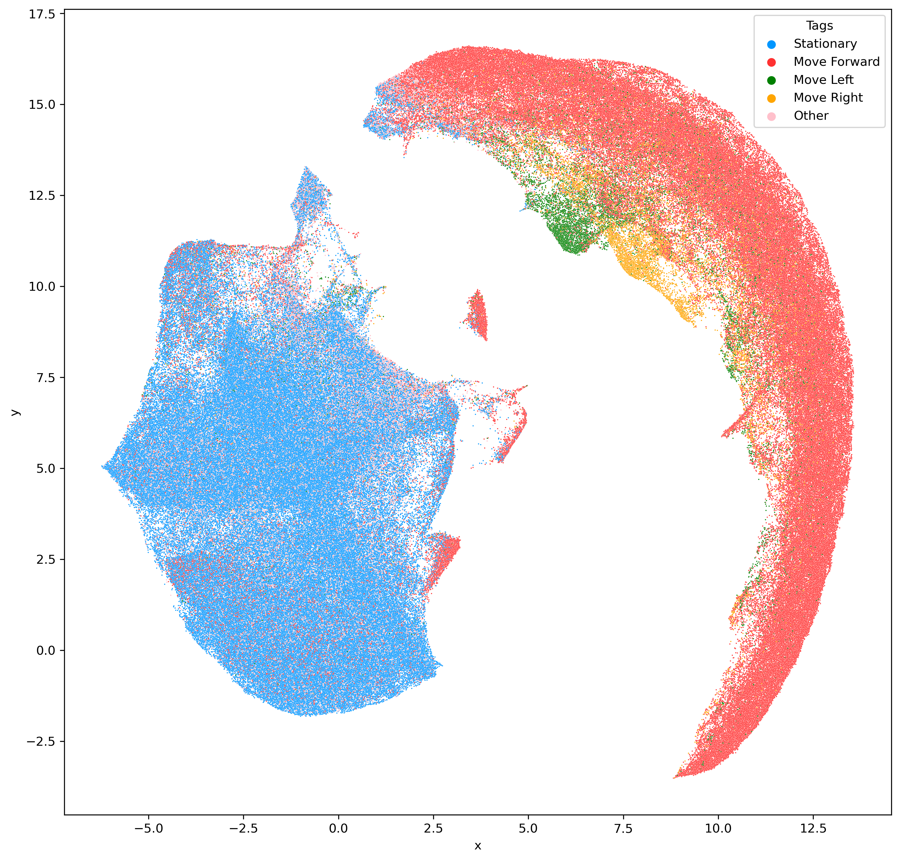
(a)

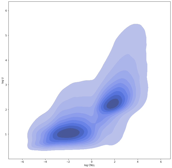
(b)

Figure 3: (left) Visualization of embeddings obtained by UMAP [20]. Blue corresponds to stationary, red, green and orange correspond to moving forward, left and right respectively, pink stands for other. (right) Logarithm of uncertainty measure against logarithm of CNLL for development dataset.

3 Experiments and Results

The model was implemented using PyTorch [21] and PyTorch Geometric [22] and trained on single RTX 3090 GPU on $50\%$ of the data with batch size of 32.

VectorNet encoder uses 3 layers of subgraph Message-Passing with hidden dimensions of 64 and transformer convolution layer with 2 attention heads of size 64. The heads are averaged instead of concatenation. Decoder has 2 transformer blocks with 4 heads and hidden dimension of 128. Feed-Forward network has 2 linear layers with intermediate dimension of 256. The inputs (state+mode embeddings) are not scaled before adding positional embeddings.

SNGP model utilizes pretrained encoder with the same parameters. We set $D_{L}=2048$, $m=0.9999$, $s=0.1$ and $l^{-1}=0.05$. Tuning these parameters could be quite tricky since SNGP is sensible to batch size and volume of data.

For all models the initial learning rate was set to $0.001$ and Adam optimizer was used. For a multimodal model we used MultiStepLR scheduler with milestones $[6,12]$ with a decay factor $0.3$ and the model was trained for a total of $20$ epochs. We pretrained VectorNet encoder for $19$ epochs with decay every 5 epochs by a factor 0.3. SNGP head was trained for a $5$ epochs. We reset covariance matrix at the end of each epoch.

The results on the evaluation data are shown in the Table 1. As it is shown on the Figure 3, there is an expected trend: higher values of CNLL correlate with high values of uncertainty measure.

Model	R-AUC CNLL	CNLL	minADE	minFDE	wADE	wFDE
VN SNGP	$2.942$	$17.037$	$0.514$	$1.001$	$1.330$	$3.167$
VNTransformer SNGP	$2.619$	$15.599$	$0.495$	$0.936$	$1.326$	$3.158$

Table 1: Results obtained by training on $50\%$ data in Shifts Challenge. VN stands for model with plain VectorNet, VNTransformer stands for model with Transformer decoder. Area under CNLL retention curve (R-AUC CNLL) [23] was used for final ranking.

4 Conclusion

We considered a composite model for multimodal trajectory prediction and uncertainty estimation in vechicle motion prediction task. The resulting model shows a good performance in multimodal task and ability to detect out-of-distribution examples.

References

- [1] Henggang Cui et al. “Multimodal Trajectory Predictions for Autonomous Driving using Deep Convolutional Networks”, 2018 arXiv:1809.10732
- [2] Fang-Chieh Chou et al. “Predicting Motion of Vulnerable Road Users using High-Definition Maps and Efficient ConvNets”, 2019 arXiv:1906.08469
- [3] Jiyang Gao et al. “VectorNet: Encoding HD Maps and Agent Dynamics from Vectorized Representation”, 2020 arXiv:2005.04259
- [4] Ming Liang et al. “Learning Lane Graph Representations for Motion Forecasting”, 2020 arXiv:2007.13732
- [5] Thomas N. Kipf and Max Welling “Semi-Supervised Classification with Graph Convolutional Networks”, 2016 arXiv:1609.02907
- [6] Petar Velickovic et al. “Graph Attention Networks”, 2017 arXiv:1710.10903
- [7] Hang Zhao et al. “TNT: Target-driveN Trajectory Prediction”, 2020 arXiv:2008.08294
- [8] Yicheng Liu et al. “Multimodal Motion Prediction with Stacked Transformers”, 2021 arXiv:2103.11624
- [9] Nemanja Djuric et al. “Uncertainty-aware Short-term Motion Prediction of Traffic Actors for Autonomous Driving”, 2020 arXiv:1808.05819v3
- [10] Sungjoon Choi, Kyungjae Lee, Sungbin Lim and Songhwai Oh “Uncertainty-Aware Learning from Demonstration using Mixture Density Networks with Sampling-Free Variance Modeling”, 2017 arXiv:1709.02249
- [11] Angelos Filos et al. “Can Autonomous Vehicles Identify, Recover From, and Adapt to Distribution Shifts?”, 2020 arXiv:2006.14911
- [12] Joost Amersfoort, Lewis Smith, Yee Whye Teh and Yarin Gal “Uncertainty Estimation Using a Single Deep Deterministic Neural Network”, 2020 arXiv:2003.02037
- [13] Jeremiah Zhe Liu et al. “Simple and Principled Uncertainty Estimation with Deterministic Deep Learning via Distance Awareness”, 2020 arXiv:2006.10108
- [14] Joost Amersfoort et al. “On Feature Collapse and Deep Kernel Learning for Single Forward Pass Uncertainty”, 2021 arXiv:2102.11409
- [15] Jakob Gawlikowski et al. “A Survey of Uncertainty in Deep Neural Networks”, 2021 arXiv:2107.03342
- [16] Andrey Malinin al “Shifts: A Dataset of Real Distributional Shift Across Multiple Large-Scale Tasks”, 2021 arXiv:2107.07455
- [17] Justin Gilmer et al. “Neural Message Passing for Quantum Chemistry”, 2017 arXiv:1704.01212
- [18] Yunsheng Shi et al. “Masked Label Prediction: Unified Message Passing Model for Semi-Supervised Classification”, 2020 arXiv:2009.03509
- [19] Ali Rahimi and Benjamin Recht “Random Features for Large-Scale Kernel Machines” In Advances in Neural Information Processing Systems 20, 2008 URL: https://proceedings.neurips.cc/paper/2007/file/013a006f03dbc5392effeb8f18fda755-Paper.pdf
- [20] Leland McInnes, John Healy and James Melville “UMAP: Uniform Manifold Approximation and Projection for Dimension Reduction”, 2018 arXiv:1802.03426
- [21] Adam Paszke et al. “PyTorch: An Imperative Style, High-Performance Deep Learning Library” In Advances in Neural Information Processing Systems 32 Curran Associates, Inc., 2019 URL: http://papers.neurips.cc/paper/9015-pytorch-an-imperative-style-high-performance-deep-learning-library.pdf
- [22] Matthias Fey and Jan Eric Lenssen “Fast Graph Representation Learning with PyTorch Geometric”, 2019 arXiv:1903.02428
- [23] Andrey Malinin “Uncertainty Estimation in Deep Learning with application to Spoken Language Assessment”, 2019