Detecting Object States vs Detecting Objects:
A New Dataset and a Quantitative Experimental Study

Abstract

The detection of object states in images (State Detection - SD) is a problem of both theoretical and practical importance and it is tightly interwoven with other important computer vision problems, such as action recognition and affordance detection. It is also highly relevant to any entity that needs to reason and act in dynamic domains, such as robotic systems and intelligent agents. Despite its importance, up to now, the research on this problem has been limited. In this paper, we attempt a systematic study of the SD problem. First, we introduce the Object State Detection Dataset (OSDD), a new publicly available dataset consisting of more than 19,000 annotations for 18 object categories and 9 state classes. Second, using a standard deep learning framework used for Object Detection (OD), we conduct a number of appropriately designed experiments, towards an in-depth study of the behavior of the SD problem. This study enables the setup of a baseline on the performance of SD, as well as its relative performance in comparison to OD, in a variety of scenarios. Overall, the experimental outcomes confirm that SD is harder than OD and that tailored SD methods need to be developed for addressing effectively this significant problem.

1 Introduction

The detection of object states in images is a problem of both theoretical and practical importance. By object state we refer to a condition of that object at a particular moment in time. Some object states are mutually exclusive (e.g., open/closed), while others may hold simultaneously (e.g., open, filled, lifted). The transition from one state to another is, typically, the result of an action being performed upon the object. The state(s) in which an object can be found determine(s) to a large degree its behavior in the context of its interaction with other objects and entities.

Apart from being a challenging task bearing some unique characteristics, object state detection (SD) is a key visual competence, as the successful interaction of an agent with its environment depends critically on its ability to solve this problem. SD is also closely related to other important computer vision and AI problems, such as action recognition and planning. Surprisingly, the amount of research on this subject remains low, especially when juxtaposed with the vast research effort that has been invested over the last years in related computer vision problems, such as object detection and image classification.

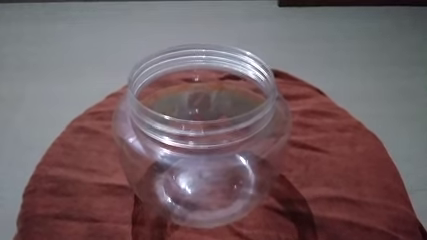
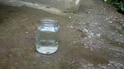
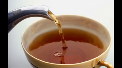
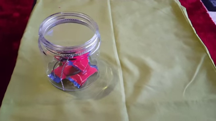
Figure 1: Each row contains objects of the same state and each column contains objects of the same class. The variance of visual appearance is significantly greater for objects of the same state than for objects of the same category.

There are several arguments that attest the significance of a solution to the SD problem. First, the detection of states is critical for decision making. In dynamic worlds, the conditions for stopping an action is state-dependent. For example, in order for a glass to be filled without an overflow its filled state must be recognized or even predicted on time. Actually, in many cases, miss-classifying the object state could be equally or even more detrimental as miss-classifying its category (e.g., recognizing a bottle as a jar vs. recognizing a filled bottle as an empty bottle). Second, inferring correctly the states of objects could facilitate significantly the recognition of actions. Conversely, the recognition of an action can provide cues about the states of objects which were affected by the action. SD is also relevant to another active and important research area, that of object affordances recognition. The inference of object affordances depends critically on their current state. For example, many different kinds of objects could be used for carrying liquids, provided that they are empty. In this case, inferring the state of the candidate container is more important that recognizing its class.

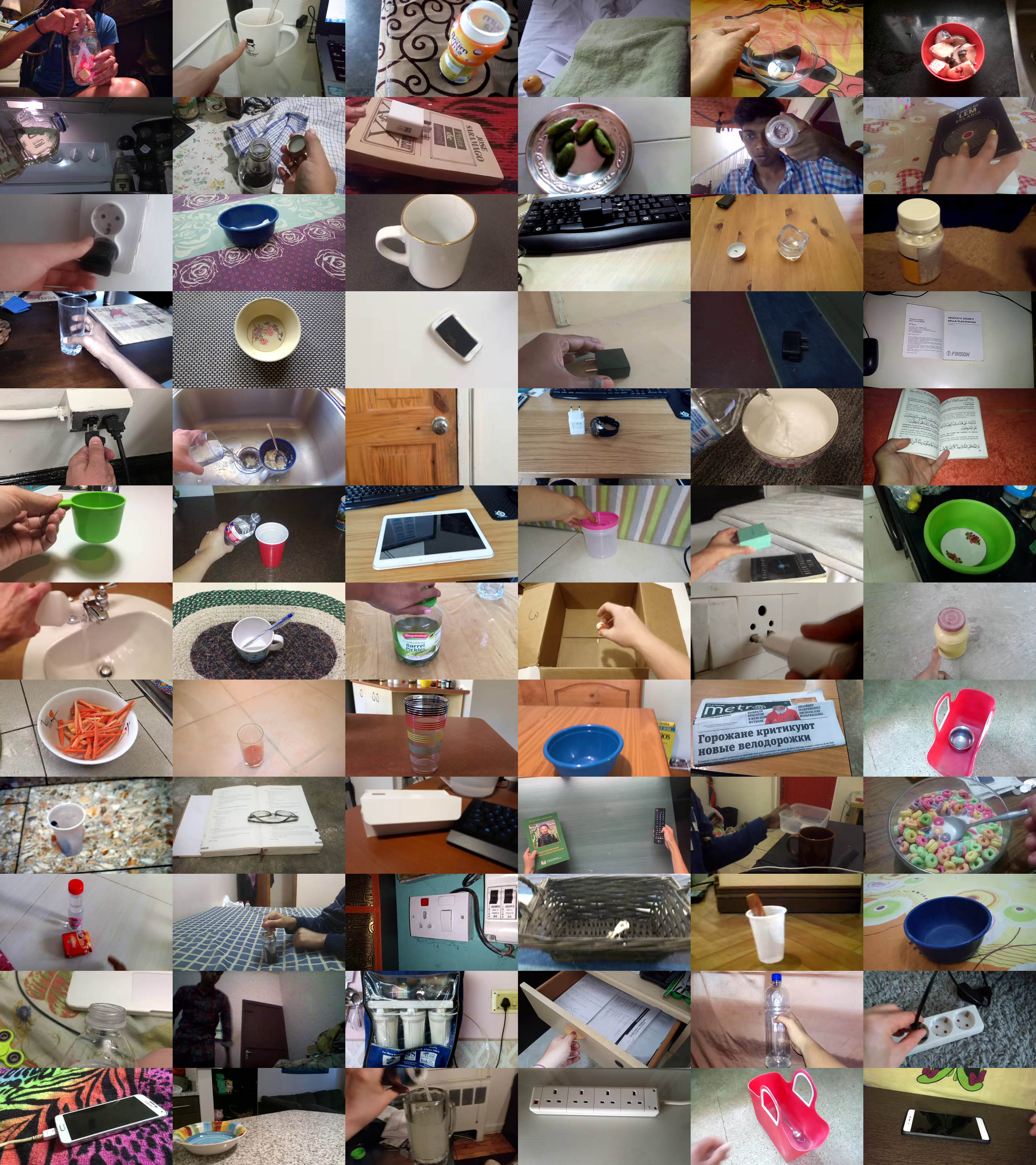
Figure 2: A small sample of the proposed OSDD dataset.

At a first glance, SD appears to be just a special case of object detection (OD). As an example, one could specialize a “box” detector to come up with an “open box” detector. This idea could explain the low levels of research activity devoted to SD, per se. However, such an approach lacks scalability as the space of all object categories times the number of their possible states is huge. Moreover, there exist some important differences between the SD and OD problems. First, the intra-class variation for object states is vastly greater than the one for objects classes. For example, objects that are visually very dissimilar such as books, bottles, boxes and drawers, may belong to the same state class (open). Figure 1 presents analogous examples. Moreover, the inter-class boundaries for the SD problem may hinge on minute details. For example, a slightly lifted cap is the only difference between an open and a closed bottle. Another special aspect of SD has to do with the fact that an object may possess, simultaneously, several non mutually exclusive states (e.g., an open, filled glass). Furthermore, considering the problem of SD under a broader perspective which also includes videos as input, we can attest the dynamic nature of object states. For example, a “filled” cup may become “empty” in seconds in contrast to its object category which remains fixed.

Motivated by the previous observations and arguments which point towards the significance and the special characteristics of SD, as well as the limited study upon the subject, we investigate the SD problem in more detail. First, we provide a new dataset, the Object States Detection Dataset (OSDD), consisting of everyday household objects appearing in a variety of different states. Given the small number of related datasets, we believe that OSDD could be useful to anyone interested in the problem of SD. Second, we conduct a number of carefully devised experiments in order to examine the performance of OD and SD on OSDD. The experimental evaluation exposes the performance of solutions to the OD and SD problems, confirming that SD is harder than OD and attesting the need for robust and performant solutions to the SD problem.

	P1	P2	P3	P4	P5
Bottle, Jar, Tub	✓	✓	✓	✗	✗
Book, Drawer, Door	✓	✗	✗	✗	✗
Basket, Box	✓	✗	✓	✗	✗
Cup, Mug, Glass, Bowl	✗	✓	✓	✗	✗
Phone, Charger, Socket	✗	✗	✗	✓	✗
Towel, Shirt, Newspaper	✗	✗	✗	✗	✓

Table 1: Objects and states in OSDD. Rows correspond clusters of object categories that may appear in the same set of states. Columns correspond to five pairs (P1-P5) of mutually exclusive states. P1: Open/Close, P2: Empty/Containing Liquid (CL), P3: Empty/Containing Solid (CS), P4: Plugged/Unplugged, P5: Folded/Unfolded.

	Open	Closed	Empty	CL	CS	Plugged	Unplugged	Folded	Unfolded	Total
basket			122		336					458
book	316	679								995
bottle	891	923	420	803	238					3275
bowl			809	146	790					1745
box	518	291	184		337					1330
charger						235	376			611
cup			432	139	220					791
door	271	481								752
drawer	468	484								952
glass			523	363	215					1101
jar	356	295	176	111	369					1307
mug			541	160	269					970
newspaper								322	135	457
phone						205	743			948
shirt								139	187	326
socket						486	1016			1502
towel								320	197	517
tub	276	153	136		416					981
Total	3096	3306	3343	1722	3190	926	2135	781	519	19018

Table 2: Number of annotations for the different object-state combinations.

Dataset	Images/Videos	Annotations	States	Objects	Task	View
OSDD (ours, proposed)	13,744 images	19,018	9	18	SD	3rd person
[Isola et al., 2015]	63,440 images	63,440	18	NA	SC	Egocentric
[Liu et al., 2017]	809 videos	330,000	21	25	SD & AR	Egocentric
[Fire and Zhu, 2017]	490 Videos	180,374	17	13	SD & AR	3rd person
[Alayrac et al., 2017]	630 Videos	19,949	7	5	SD & AR	3rd person

Table 3: OSDD and existing object states datasets, in numbers.

2 Related Work

We review existing approaches to the OD and SD problems. For OD the literature is vast and its detailed review is beyond the scope of this paper. Therefore, we restrict ourselves to an overview of the main classes of approaches that follow the more recent, state-of-art deep-learning paradigm. We also provide pointers to existing object states datasets and we identify the contributions of this work.

Object Detection: Deep learning-based object detection frameworks can be categorized into two groups: (i) one-stage detectors, such as YOLO [Redmon and Farhadi, 2017] and SSD [Liu et al., 2016] and (ii) two-stage detectors, such as Region-based CNN (R-CNN) [Girshick, 2015] and Pyramid Networks [Lin et al., 2017a]. Two-stage detectors use a proposal generator to create a sparse set of proposals in order to extract features from each proposal which are followed by region classifiers that make predictions about the category of the proposed region, whereas one-stage detectors generate categorical predictions of objects on each location of the feature maps omitting the cascaded region classification procedure. Two-stage detectors are typically more performant and achieve state-of-the-art results on the majority of the public benchmarks, while one-stage detectors are characterized by computational efficiency and are used more widely for real-time OD. Some other highly influential works in the field are [He et al., 2016], [Huang et al., 2017], [He et al., 2017] and [Lin et al., 2017b].

State Detection: The research that has been conducted in SD has treated the problem using either videos or images as input. In the first case, the problem of SD usually serves as a stepping stone to achieve action recognition.

In [Alayrac et al., 2017], SD is studied in the context of videos containing manipulation actions performed upon 7 classes of objects. The authors formulate SD as a discriminative clustering problem and attempt to address it by optimization methods. [Liu et al., 2017] represent state-altering actions as concurrent and sequential object fluents (states) and utilize a beam search algorithm for fluent detection and action recognition. In a similar vein, [Aboubakr et al., 2019] explores state detection in tandem with action recognition. The method is based on the learning of appearance models of objects and their states from video frames which are used in conjunction with a state transition matrix which maps action labels into a pre-state and a post-state. In [Isola et al., 2015], the states and transformations of objects/scenes on image collections are studied, and the learned state representations are extended to different object classes. [Fire and Zhu, 2015, Fire and Zhu, 2017] examines the causal relations between human actions and object fluent changes. [Fathi and Rehg, 2013] developed a weakly supervised method to recognize actions and states of manipulated objects before and after the action proposing a weakly supervised method for learning the object and material states that are necessary for recognizing daily actions. [Wang et al., 2016] designed a Siamese network to model precondition states, effect states and their associate actions. [Bertasius and Torresani, 2020] leveraged the semantic and compositional structure of language by training a visual detector to predict a contextualized word embedding of the object and its associated narration enabling object representation learning where concepts relate to a semantic language metric.

Scenario	Obj.	States	Nets	Exp.	Tasks
OOOS	1	2 ME	28	28	SD
MOOS	3-6	2 ME	5	5	SD
OOMS	1	3-5	8	8	SD
MOMS	18	9	1	1	SD
ODS	18	9	1	1	OD
TOOS	2	2 ME	28	7	SD, OD
SDG	3-9	2 ME	0	5	SD

Table 4: The experimental details of the different scenarios. Columns show the scenario name, number of involved objects, number of involved states (ME: mutually exclusive), number of trained networks, number of performed experiments, target problem.

Overall, previous works dealt with the SD problem mostly by employing egocentric videos. These are less challenging than 3rd person-view input due to the higher resolution in which objects are imaged and the lack of considerable clutter/occlusions. Additionally, in the majority of the cases, SD is considered a means for achieving AR and not as a goal on its own right, thus the studies of the SD problem are of a limited scope.

Object States Datasets: Currently, there are only a few object states datasets available to the research community. The MIT-States dataset [Isola et al., 2015] is composed of 63,440 images involving 115 attribute classes and 245 object categories and is suitable for state classification (SC). However, the dataset contains segmented images of objects in white background so they are far from being natural. Additionally, most of the 115 reported attributes constitute object properties that are not necessarily object states. [Liu et al., 2017] presents a dataset consisting of 809 videos covering 21 state classes and 25 object categories. The scope of the dataset is SD and action recognition (AR). The dataset presented in [Alayrac et al., 2017] contains 630 videos concerning 7 state classes and 5 object categories, also suited for SD and AR. Finally, [Fire and Zhu, 2017] proposes a RGBD video dataset for causal reasoning spanning 13 object and 17 state categories.

In general, the existing SD datasets lack the diversity that characterizes the OD datasets, which can be attributed to the fact that they have been created without having the task of SD as a primary goal.

Our contribution: We introduce OSDD, a new states dataset of 13,744 images and 19,018 states annotations. The dataset involves 18 object categories that may appear in 9 different state classes. The images of the dataset are characterised by a great variety regarding viewing angles, background and foreground scene settings, object sizes and object-state combinations. These characteristics render the dataset more challenging than most of the existing datasets which contain a much more limited diversity with respect to the aforementioned characteristics. Moreover, OSDD could be proven useful for those who want to assess the performance of approaches addressing the tasks of zero-shot and few-shot recognition.

Metric	OOOS	MOOS	OOMS	MOMS
Weighted AP	68.4	63.2	54.3	46.6
Best perf. (%)	58.0	38.0	2.0	2.0
Worst perf. (%)	6.0	6.0	14.0	74.0
Avg mAP	62.3	56.5.0	46.8	38.4
Avg AP@50:5:95	40.5	39.7	29.1	23.7

Table 5: Aggregate results for scenarios OOOS, MOOS, OOMS and MOMS. Row 1: weighted AP, row 2: percentage of experiments in which this scenario achieved best AP, row 3: percentage of experiments in which this scenario achieved worst AP, row 4: Average mAP , row 5: Average AP@50:5:95. Blue/red font indicates best/worst performance in a line.

In addition, we provide an extensive quantitative, experimental evaluation of several aspects of the SD problem. We conduct 55 different experiments including 71 differently trained networks in the context of 7 scenarios of varied settings which allows us to draw valuable insights about the nature of SD and its relation to OD. OSDD and the associated experiments set useful baselines for assessing progress on the topic of SD. To the best of our knowledge, our work is the first in which such a thorough investigation of the SD task is performed.

3 The Object States Detection Dataset (OSDD)

The proposed Objects States Detection Dataset (OSDD) consists of images depicting everyday household objects in a number of different states. The ground-truth annotations involve the labels and bounding boxes spanning 18 object categories and 9 state classes. The object categories are: bottle, jar, tub, book, drawer, door, cup, mug, glass, bowl, basket, box, phone, charger, socket, towel, shirt and newspaper. The 9 state classes are: open, close, empty, containing something liquid (CL), containing something solid (CS), plugged, unplugged, folded and unfolded.

The states are grouped in 5 pairs of mutually exclusive states. Table 1 shows which cluster of objects is relevant to which pair of mutually exclusive (ME) states. Table 2 provides an overview of the dataset contents. For all object categories (rows) and states (columns), we report the number of annotations.

State	OOOS	MOOS	OOMS	MOMS
Open	68.7	67.4	52.4	49.9
Closed	69.2	62.2	62.4	48.2
Empty(vs CL)	70.0	67.6	58.3	56.4
Filled	49.9	40.4	38.4	25.0
Empty(vs CS)	73.0	69.8	58.3	56.4
Occupied	64.8	56.0	53.6	37.2
Folded	57.3	62.0	NA	39.5
Unfolded	37.0	39.9	NA	22.7
Connected	60.3	49.2	NA	24.8
Unconnected	84.9	78.5	NA	66.1

Table 6: Experimental results for the AP metric averaged at the level of states for the OOOS, MOOS, OOMS and MOMS scenarios. Each row corresponds to a different state. Blue/red font indicates best/worst performance for the given state.

The images were obtained by selecting video frames from the something-something V2 Dataset [Mahdisoltani et al., 2018]. Specifically, images containing visually salient objects and states of the aforementioned categories were captured and annotated with bounding-boxes and ground truth labels referring to the corresponding object categories and state classes. Overall, the dataset contains 13,744 images and 19,018 annotations obtained by selecting the first, last and middle frames of 9,015 videos, after checking that each of them contains salient information. There are more annotations than images because (a) in a certain image there may be more than one objects or/and (b) a certain object is annotated for all the non-exclusive states it appears in.

The dataset annotation was performed based on the Computer Vision Annotation Tool (CVAT). In order to handle properly ambiguous situations and safeguard from erroneous annotations, each image was examined at least five times. Overall, the annotation process required approximately 350 person hours.

Object	OOOS	MOOS	OOMS	MOMS
bottle	61.9	50.0	40.2	32.4
tub	74.8	48.1	47.0	18.9
cup	70.8	73.2	66.5	64.7
mug	78.0	80.3	82.6	71.4
jar	50.8	59.3	36.0	30.6
glass	64.2	62.6	55.9	50.0
bowl	75.5	77.3	71.5	68.0
box	73.4	71.2	59.6	62.9
basket	58.6	65.6	NA	55.2
book	74.7	63.9	NA	62.0
door	45.9	45.4	NA	30.7
shirt	40.4	33.3	NA	22.8
newspaper	40.5	45.8	NA	14.5
towel	54.7	62.4	NA	44.1
drawer	73.8	66.5	NA	58.5
phone	79.2	79.2	NA	70.0
charger	69.5	38.7	NA	35.2
socket	80.3	75.8	NA	51.9

Table 7: Experimental Results for the AP metric averaged at the level of states for the OOOS, MOOS, OOMS and MOMS scenarios. Each row corresponds to a different object. Blue/red font indicates best/worst performance for the given object.

3.1 OSDD vs existing object states datasets

Table 3 summarizes information regarding the existing SD datasets. The dataset that is most similar to OSDD is the one presented in [Isola et al., 2015]. However, the two datasets differ in a number of ways. First, the images in our dataset are snapshots of video tracklets that show objects manipulations, whereas the images in [Isola et al., 2015] stem from scrapping. Moreover, the majority of images in [Isola et al., 2015] are cropped containing a single object, whereas OSDD images contain objects in context (e.g., other objects, background, etc).

Another important remark regarding the existing datasets, is that in the case of [Liu et al., 2017], [Fire and Zhu, 2017] and [Alayrac et al., 2017], annotations were provided for adjacent video frames, whereas in our case they involve the first, middle and last frames of 9,015 videos. Thus, although they appear to provide many more annotations, they are much less diverse than OSDD due to the similarity between many of the annotated frames.

In summary, the aspects that distinguish OSDD from the existing datasets are its greater diversity regarding objects and states appearance, the greater background/foreground variation and the greater diversity of viewpoints which results in a vast variety of object sizes and viewing angles. These characteristics make it unique for studying SD in challenging, realistic scenarios.

Object	Pair	OOOS	MOOS	OOMS	MOMS
bottle	P1	71.5 / 48.0	67.7 / 46.8	40.4 /  25.3	38.4 / 23.7
	P2	38.0 /  26.3	24.4 / 15.1
	P3	68.6 / 43.8	43.8 / 30.1
jar	P1	50.0 /  25.8	67.2 / 49.8	33.9 /  22.3
	P2	35.8 / 25.0	52.2 / 33.7
	P3	51.8 /  33.4	52.6 /  38.9
tub	P1	83.0 / 59.1	57.5 / 42.4	41.9 / 23.2
	P2	44.5 /  25.3	66.6 / 37.5
	P3	64.2 /  39.7	29.4 /  20.6
box	P1	73.0 /  53.4	61.1 / 46.2	56.7 /  20.7
	P3	67.2 /  43.8	60.4 /  45.0
glass	P2	60.1 /  41.5	52.4 /  34.9	46.8 / 32.9
	P3	57.9 /  41.0	63.7 /  47.7
cup	P2	59.9 /  41.6	54.5 /  36.6	53.5 / 36.5
	P3	62.2 /  47.8	75.0 /  60.0
mug	P2	56.1 /  36.6	56.4 /  36.9	64.8 / 50.1
	P3	64.6 /  45.8	73.7 /  56.3
bowl	P2	57.0 /  40.6	78.7 /  64.5	54.9 / 35.5
	P3	74.9 /  52.4	59.8 /  41.8
basket	P3	55.6 /  29.1	53.6 /  41.6	NA
phone	P4	61.7 /  40.6	64.2 /  40.6	NA
charger	P4	68.6 /  42.2	38.1 /  21.4	NA
socket	P4	76.2 /  39.3	71.0 /  36.1	NA
book	P1	64.2 /  44.3	57.0 /  42.7	NA
door	P1	42.1 /  23.9	39.1 /  23.8	NA
drawer	P1	75.6 /  43.9	68.9 /  45.8	NA
newspaper	P5	35.7 /  23.5	43.7 /  29.8	NA
towel	P5	53.9 /  35.5	61.5 /  41.6	NA
shirt	P5	41.8 /  22.5	36.5 /  25.6	NA
Weighted Average		62.3 / 40.5	56.5 / 39.7	46.8 / 29.1	38.4 / 23.7

Table 8: Experimental results for the OOOS, MOOS, OOMS and MOMS scenarios. First number in each cell corresponds to the mAP metric and second number corresponds to the AP@50:5:95 metric respectively. The metrics are calculated at the level of each object pairs for the OOOS and MOOS scenarios, at the level of each object for the OOMS scenario and at the level of all objects for the MOMS scenario respectively. Blue/red font indicates best/worst performance between the OOOS and MOOS scenarios.

Figure 3: AP for the OOOS, MOOS, OOMS and MOMS scenarios, for each object state in OSDD.

Metric	MOMS	ODS
AP@50:5:95	23.7	30.9
mAP	38.4	48.8

Table 9: Experimental results for the MOMS and ODS scenarios. See text for details.

Scenario Details				Results
Object 1	Object 2	State 1	State 1	CS1	CS 2	ST	CO1	CO2	OB
bottle	jar	open	closed	19.5 /13.3	9.0 / 5.4	27.2 /17.6	26.7 /18.1	69.7 / 45.5	67.3 / 45.5
bottle	jar	empty	CL	7.7 /5.0	1.5 / 0.7	35.2 /20.7	52.1 /28.0	38.2 /20.9	58.8 / 33.4
cup	glass	empty	CL	2.4 / 1.6	2.6 /1.8	55.0 /39.4	59.2 /43.2	49.8 /26.9	79.8 / 44.6
cup	glass	empty	CS	4.4 / 3.0	10.6 /7.4	59.7 /43.3	37.3 /24.1	56.1 /28.1	75.4 / 54.6
charger	phone	plugged	unplugged	5.7 /3.3	4.7 / 3.0	49.4 /28.3	49.9 /30.8	67.0 /33.8	81.7 / 45.9
shirt	towel	unfolded	folded	19.7 /14.4	13.0 / 7.2	32.5 /19.2	45.4 /28.3	51.4 /27.3	60.3 / 37.4
newspaper	towel	unfolded	folded	0.3 / 0.2	3.6 /2.4	77.1 / 58.6	72.4 /51.0	41.0 /21.6	84.4 /54.4
bowl	mug	empty	CL	5.2 / 3.5	18.6 /11.5	50.1 /32.3	34.1 /25.2	61.5 /37.9	83.9 / 67.2
bowl	mug	empty	CS	6.8 / 4.8	21.5 /14.0	46.0 /35.0	14.3 /9.2	67.6 /39.6	77.7 / 48.6
door	drawer	open	closed	1.5 /1.0	1.5 / 0.6	19.8 /10.5	16.7 /7.6	61.3 /39.5	67.3 / 39.9
glass	mug	empty	CL	1.1 /0.7	0.8 / 0.6	74.8 /52.6	72.1 /56.1	54.1 /38.4	85.3 / 56.5
glass	mug	empty	CS	3.3 /2.4	2.9 / 2.2	55.4 /42.1	43.7 /31.6	61.8 /43.7	78.4 / 53.8
Weighted Average mAP				8.5	6.4	53.3	49.0	48.0	72.5
Best perf (%)				0.0	0.0	0.0	0.0	14.3	85.7
Worst perf. (%)				42.9	57.1	0.0	0.0	0.0	0.0
Weighted Average AP@50:5:95				5.8	4.0	29.2	32.5	31.9	45.1
Best perf. (%)				0.0	0.0	14.3	0.0	14.3	71.4
Worst perf. (%)				42.9	57.1	0.0	0.0	0.0	0.0

Table 10: Experimental results for the TOOS Scenario. Each row corresponds to a different objects/states combinations. First number in each cell corresponds to the mAP metric and second number corresponds to the AP@50:5:95 metric respectively. Blue/red font indicates best/worst performance achieved for the given objects/states combination.

4 Experimental Evaluation

OD has been studied extensively and it is one of the most prominent cases where the standard deep learning approach, i.e. the training of special architectures of Deep Neural Networks with appropriately annotated datasets, has been proven exceptionally advantageous in comparison to traditional techniques involving hand-crafted image features. We choose to follow the same approach for solving SD, since it allows to assess our intuition regarding the nature of OD and SD, both directly and indirectly. Specifically, we can observe how the performance of SD variants changes as the complexity of the problem at hand varies, and check whether this behavior is congruent to the one that is expected for OD variants when undergo a similar complexity shift. Equally importantly, by testing SD under the same experimental conditions (i.e., identical training samples and network architectures) that were used for an OD problem, we can compare directly the performances obtained for the two tasks.

Training configuration: The network we are using in our experimental evaluation is Yolov4 [Bochkovskiy et al., 2020], one of the most popular CNNs for OD. We opted for using this network because it it can be easily fine-tuned, it has been utilized with much success in a wide variety of settings and exhibits SoA performance in OD. Consequently, we follow the typical procedure for the deployment of a network tailored for OD, i.e., we split the set of the annotated image samples into training, validation and testing parts.

In order to accelerate the training phase and boost the performance, we follow the common practice of using pre-trained weights at the start of the training phase of every network. Specifically, the weights used are obtained after training with MS-COCO dataset [Lin et al., 2014].

We also employ data augmentation by horizontally flipping all frames in a batch with a probability of 0.5. The number of training epochs is set equal to the product of 2,000 to the number of the categories of the corresponding sub-task. We used the Adam optimizer with an initial learning rate of 0.001 and an early stopping policy of 50 epochs.

Evaluation metrics: Given an image as an input, the solution of the SD problem produces the bounding box of each detected object and the set of state classes, in which that object belongs. For a detection to be considered correct, the set of states must be identical to the ground truth and the overlap between the ground truth and the detected bounding boxes must be greater than a certain threshold, which, following common practices, we set to 50%. Moreover, predictions having confidence lower than 50% are rejected. Our analyses are based on three standard performance metrics used for assessing OD tasks: AP, AP@50:5:95 and mAP. AP is calculated for each object-state combination in each experiment instance, whereas AP@50:5:95 and mAP are calculated per experiment instance as in [Padilla et al., 2020].

Experimental scenarios: For the purposes of the evaluation, we devise 7 different scenarios, each one involving different assumptions regarding the object categories and states which are to be detected. The details of the scenarios are presented in Table 4. In the rest of this section, we describe each scenario, we explain the rationale behind it along with the hypotheses that we want to test, and present the experimental results we obtained and the conclusions that we draw.

4.1 The OOOS, MOOS, OOMS and MOMS scenarios

Aiming to explore how the approach fares as the complexity of the problem scales, we devise 4 different SD experimental scenarios. The adjustable settings for the scenarios concern the number of different object categories involved and the number of possible states for each object category. Specifically, the tested SD scenarios are defined as follows:

• OOOS (One Object One State pair): Involves the detection of an object’s state, assuming the object class is known, i.e. the corresponding network has been trained exclusively on objects belonging to this class, and the possible states for the object are two and mutually exclusive (M.E.).

• MOOS (Many Objects One State pair): involves the detection of an object’s state when its class is not known, i.e. the number of object classes upon which the corresponding network has been trained is more than one, and the possible states for the objects are two and M.E.

• OOMS (One Object Many States): involves the detection of an object’s state(s) assuming the object class is known and the possible states for the object are more than two and not necessarily M.E.

• MOMS (Many Objects Many States): Detection of an object’s state when its class is not known beforehand and the possible states for each class of object could be more than two and not necessarily M.E.

The obtained results are summarized in Tables 5-8. It can be verified that the best performance is obtained in the OOOS scenario, while the worst in the MOMS scenario. This is expected, as from a single object and state pair (OOOS) we move into the far more complex scenario of multiple objects and multiple state pairs (MOMS). However, we also observe that performances in MOOS are considerably better that performances in OOMS. Thus, when departing from the baseline OOOS scenario and increasing the complexity of the problem either in the direction of adding more objects (MOOS) or in the direction of adding more states (OOMS), we observe that the addition of more states makes the problem considerably harder.

	State 1	State 2
Object 1	(A) $O_{1},S_{1}$	(B) $O_{1},S_{2}$
Object 2	(C) $O_{2},S_{1}$	(D) $O_{2},S_{2}$

Table 11: Object/state combinations in the TOOS scenario. See text for details.

Setting	Training	Testing	Task
Cross States 1 (CS1)	A, D	B, C	SD
Cross States 2 (CS2)	B, C	A, D	SD
States (ST)	A, B, C, D	A, B, C, D	SD
Cross Objects 1 (CO1)	A, D	B, C	OD
Cross Objects 2 (CO2)	B, C	A, D	OD
Objects (OB)	A, B, C, D	A, B, C, D	OD

Table 12: Dataset splits in each setting of the TOOS scenario. A, B, C and D are defined in Table 11. See text for details.

	Book	Bottle	Box	Door	Drawer	Jar	Tub
book	64.2 / 44.3	1.2 /0.6	22.3 /16.7	3.4 /2.0	1.1 / 0.5	2.3 /1.4	9.9 /5.4
bottle	11.7 /6.9	71.5 / 48.0	5.6 /3.8	0.0 / 0.0	0.9 /0.8	46.3 /30.4	14.1 /9.3
box	35.1 /22.8	4.1 /2.7	73.0 / 53.4	5.1 / 1.7	28.9 /13.6	11.0 /6.7	59.5 /42.7
door	2.6 /1.6	0.1 / 0.0	4.0 /1.6	42.1 / 23.9	5.1 /1.5	0.0 / 0.0	0.7 /0.5
drawer	17.4 /7.4	0.1 / 0.0	9.8 /4.6	8.2 /5.0	75.6 / 43.9	0.0 / 0.0	0.0 / 0.0
jar	1.7 /1.0	14.0 /7.1	1.9 /1.1	0.0 / 0.0	0.4 /0.1	50.0 / 25.8	21.2 /11.0
tub	4.8 /2.4	2.1 /1.3	15.9 /10.6	0.2 / 0.1	4.6 /2.0	26.7 /19.0	83.0 / 59.1

Table 13: Experimental results for the SDG scenario, for the mutually exclusive states pair P1. The first number in each cell corresponds to the mAP metric and the second to the AP@50:5:95 metric respectively.

	bottle	bowl	cup	glass	jar	mug
bottle	38.0 / 26.3	1.6 / 0.9	7.0 /4.2	5.7 /3.3	19.1 /11.3	2.0 /1.4
bowl	0.5 / 0.4	57.0 / 40.6	35.4 /25.5	13.1 /9.2	9.6 /6.9	29.9 /17.2
cup	1.1 / 0.8	46.8 /33.1	59.9 /41.6	34.9 /25.5	25.3 /17.7	63.3 / 47.5
glass	1.3 / 0.8	20.6 /15.9	33.5 /25.3	60.1 / 41.5	19.7 /14.9	14.4 /7.7
jar	10.7 /5.1	2.4 / 1.2	4.0 /2.1	26.3 /13.6	35.8 / 25.0	5.6 /2.6
mug	0.4 / 0.2	46.3 /32.8	52.1 /35.7	31.3 /20.2	15.4 /10.0	56.1 / 36.6

Table 14: Experimental results for the SDG scenario, for the mutually exclusive states pair P2. The first number in each cell corresponds to the mAP metric and the second to the AP@50:5:95 metric respectively. Blue/red font indicates best/worst performance in a line.

	basket	bottle	bowl	box	cup	glass	jar	mug	tub
basket	55.6 / 29.1	17.4 /10.0	22.4 /15.7	29.9 /20.5	17.4 /12.6	10.2 / 5.8	10.3 /7.4	16.2 /10.4	23.6 /13.2
bottle	5.5 /3.4	68.6 / 43.8	15.3 /8.9	4.0 / 2.6	32.9 /22.3	31.0 /20.1	41.4 /27.6	11.9 /6.4	17.9 /10.1
bowl	46.1 /34.8	8.7 /4.8	74.9 / 52.4	5.7 / 2.3	49.7 /37.7	16.6 /10.4	13.9 /8.9	32.1 /17.9	30.1 /20.1
box	42.2 /21.3	17.5 /9.1	42.8 /18.9	67.2 / 43.8	47.2 /22.0	18.9 /9.5	20.5 /10.4	17.2 / 9.0	39.4 /18.5
cup	37.1 /23.5	7.4 /5.1	47.7 /31.2	8.2 / 4.2	62.2 / 47.8	43.0 /29.1	21.4 /15.1	65.0 /41.5	19.8 /13.1
glass	17.4 /10.4	10.4 /4.6	25.7 /15.2	3.1 / 1.5	41.4 /25.0	57.9 / 41.0	17.9 /10.1	24.5 /12.7	11.9 /7.1
jar	9.2 / 5.5	24.0 /16.4	21.1 /15.3	15.0 /9.4	22.5 /14.7	22.0 /14.8	51.8 / 33.4	14.1 /9.7	20.5 /11.7
mug	16.2 /11.3	11.6 /7.3	55.1 /37.9	0.7 / 0.6	61.0 /42.9	28.9 /19.3	12.3 /8.2	64.6 / 45.8	15.6 /10.1
tub	31.8 /18.5	27.2 /15.8	64.9 /38.2	19.5 / 10.1	44.6 /30.8	21.8 /12.6	31.1 /18.4	27.2 /14.5	64.2 / 39.7

Table 15: Experimental results for the SDG scenario, for the mutually exclusive states pair P3. The first number in each cell corresponds to the mAP metric and the second to the AP@50:5:95 metric respectively. Blue/red font indicates best/worst performance in a line.

	charger	phone	socket		newspaper	shirt	towel
charger	68.6 / 42.2	12.6 /7.8	3.1 / 0.7	newspaper	35.7 / 23.5	6.9 / 4.3	12.2 /8.0
phone	22.4 /9.5	61.7 / 40.6	0.0 / 0.0	shirt	11.0 / 5.1	41.8 / 22.5	25.5 /18.5
socket	4.0 /0.9	0.0 / 0.0	76.2 / 39.3	towel	19.7 / 12.7	34.0 /23.5	53.9 / 35.5

Table 16: Experimental results for the SDG scenario, for the mutually exclusive states pair P4 (left table) and P5 (right table) respectively. The first number in each cell corresponds to the mAP metric and the second to the AP@50:5:95 metric respectively. Blue/red font indicates best/worst performance in a line

4.2 Object Detection Scenario (ODS) vs MOMS

The Object Detection Scenario (ODS) deals with the detection of object categories, using the same settings used for the MOMS scenario. Essentially, it is about the same data, processed with the same network architectures, with the exception that in ODS we seek for the object categories, while in MOMS we seek for the object states.

The performances of the detectors for the two scenarios are presented in Table 9. We observe that the performance in OD is better than that achieved in SD. The better ODS performance is obtained despite the fact that ODS has to deal with double the number of categories (18) compared to MOMS (9). Furthermore, the existence of visually similar pairs of objects (bottle-jar, cup-glass, towel-shirt) increase the difficulty of the OD task. Overall, the comparison between the performances of the two scenarios supports strongly the notion that SD is a harder problem to solve than OD.

4.3 The Two Objects One State pair (TOOS) scenario

In the context of the Two Objects One State Pair (TOOS) scenario, we train and test for images in which there are two different types of objects appearing in either one of two mutually exclusively states. Specifically, let $O_{1}$ and $O_{2}$ be the two objects and $S_{1}$ and $S_{2}$ the two states. The situation is illustrated in Table 12. We define six different cases, depending on which subset of data is used for training, which for testing and what task is solved. All these splits have been employed in 12 different object/states combinations. The rationale behind these experiments is to compare directly the learning capacity of the detectors for object classes and object categories, when trained and tested on exactly the same base of data.

Table 10 summarizes the obtained results. The performance in CS1 and CS2 (aiming for states) is significantly inferior to the one observed in cases CO1 and CO2 (aiming for objects). The poor performance in this case can be explained by the fact that the detectors learn principally the visual features of the object category and not the ones of the state class. In other words, the category of an object is visually much more salient than its state. Additionally, the performance in ST is lower than the performance on OB. This evidence supports the hypothesis that SD is harder than OD.

4.4 State Detection Generalization (SDG) scenario

In the State Detection Generalization Scenario (SDG), we examine the generalization capacity of the state detectors. Specifically, in the context of this scenario, state detectors which have been trained for instances of one particular object category and a pair of two mutually exclusive states are tested on instances of other categories of objects that appear on either one of the same two mutually exclusively states. As an example, we check whether an SD method trained on bottles to detect whether they are filled or empty, is used to check whether a glass is filled or empty. In this case, we expect that the detectors will be able to generalize better for objects that are visually similar to the object class for the states of which they have been trained.

The results for this scenario for the pair P1 of states Open/Close, is shown in Tables 13-16. The obtained results corroborate the intuition that the performance of a state detector increases along with the visual similarity between the objects classes of the trained and the tested samples. In more detail, the performances are high for specific cases of great visual similarity and mediocre or poor for the rest of the cases. The fact that the state detectors can only generalize for certain cases makes probable that the state detectors will exhibit poor performance when encountering new types of objects. The above conclusions are consistent with the ones obtained from all the rest experiments performed on the rest of mutually exclusive pairs of states (P2-P5), the results of which are reported in the supplementary material.

5 Summary and Future Work

In this paper, we have introduced a new dataset of object states and conducted an extensive series of experiments over it in order to compare the SD and OD tasks. Overall, the experimental results indicate the significant differences of the SD and OD tasks. SD is more challenging than OD. Moreover, the results obtained for more than a single pair of state classes can be considered mediocre to poor. In this case, better performance could be obtained if a number of OOOS or MOOS detectors are employed simultaneously but the scalability issues of this approach limit its practical use.

Regarding future work, there are a number of steps worth exploring. First, a more fine-grained categorization of the states would be more convenient especially for SDs used in the context of AR. Moreover, an experimental evaluation using a two-stage SoA object detector, such as Faster-RCNN [Ren et al., 2015], could provide additional insights with respect to the similarities and differences between SD and OD. The utilization of semantic embeddings, which have been used with great success in challenging problems such as Zero-Shot recognition, is another avenue that seems promising. Another interesting avenue of research would be to examine how the grouping of objects according to common sense criteria affects the performance of the state detectors. Obviously, the main goal is to come up with a novel method for SD which will cope with this important and difficult problem in realistic conditions.

References

- Aboubakr et al., 2019 Aboubakr, N., Crowley, J. L., and Ronfard, R. (2019). Recognizing Manipulation Actions from State-Transformations.
- Alayrac et al., 2017 Alayrac, J.-B., Sivic, J., Laptev, I., and Lacoste-Julien, S. (2017). Joint Discovery of Object States and Manipulation Actions. In International Conference on Computer Vision (ICCV).
- Bertasius and Torresani, 2020 Bertasius, G. and Torresani, L. (2020). COBE: Contextualized Object Embeddings from Narrated Instructional Video. pages 1–14.
- Bochkovskiy et al., 2020 Bochkovskiy, A., Wang, C.-Y., and Liao, H.-Y. M. (2020). Yolov4: Optimal speed and accuracy of object detection. arXiv preprint arXiv:2004.10934.
- Fathi and Rehg, 2013 Fathi, A. and Rehg, J. M. (2013). Modeling actions through state changes. Proceedings of the IEEE Computer Society Conference on Computer Vision and Pattern Recognition, pages 2579–2586.
- Fire and Zhu, 2015 Fire, A. and Zhu, S. C. (2015). Learning perceptual causality from video. ACM Transactions on Intelligent Systems and Technology, 7(2).
- Fire and Zhu, 2017 Fire, A. and Zhu, S.-C. (2017). Inferring hidden statuses and actions in video by causal reasoning. In Proceedings of the IEEE Conference on Computer Vision and Pattern Recognition Workshops, pages 48–56.
- Girshick, 2015 Girshick, R. (2015). Fast r-cnn. In Proceedings of the IEEE international conference on computer vision, pages 1440–1448.
- He et al., 2017 He, K., Gkioxari, G., Dollár, P., and Girshick, R. (2017). Mask r-cnn. In Proceedings of the IEEE international conference on computer vision, pages 2961–2969.
- He et al., 2016 He, K., Zhang, X., Ren, S., and Sun, J. (2016). Deep residual learning for image recognition. In Proceedings of the IEEE conference on computer vision and pattern recognition, pages 770–778.
- Huang et al., 2017 Huang, G., Liu, Z., Van Der Maaten, L., and Weinberger, K. Q. (2017). Densely connected convolutional networks. In Proceedings of the IEEE conference on computer vision and pattern recognition, pages 4700–4708.
- Isola et al., 2015 Isola, P., Lim, J. J., and Adelson, E. H. (2015). Discovering states and transformations in image collections. Proceedings of the IEEE Computer Society Conference on Computer Vision and Pattern Recognition, 07-12-June:1383–1391.
- Lin et al., 2017a Lin, T.-Y., Dollár, P., Girshick, R., He, K., Hariharan, B., and Belongie, S. (2017a). Feature pyramid networks for object detection. In Proceedings of the IEEE conference on computer vision and pattern recognition, pages 2117–2125.
- Lin et al., 2017b Lin, T.-Y., Goyal, P., Girshick, R., He, K., and Dollár, P. (2017b). Focal loss for dense object detection. In Proceedings of the IEEE international conference on computer vision, pages 2980–2988.
- Lin et al., 2014 Lin, T.-Y., Maire, M., Belongie, S., Hays, J., Perona, P., Ramanan, D., Dollár, P., and Zitnick, C. L. (2014). Microsoft coco: Common objects in context. In European conference on computer vision, pages 740–755. Springer.
- Liu et al., 2016 Liu, W., Anguelov, D., Erhan, D., Szegedy, C., Reed, S., Fu, C.-Y., and Berg, A. C. (2016). Ssd: Single shot multibox detector. In European conference on computer vision, pages 21–37. Springer.
- Liu et al., 2017 Liu, Y., Wei, P., and Zhu, S. C. (2017). Jointly Recognizing Object Fluents and Tasks in Egocentric Videos. Proceedings of the IEEE International Conference on Computer Vision, 2017-Octob:2943–2951.
- Mahdisoltani et al., 2018 Mahdisoltani, F., Berger, G., Gharbieh, W., Fleet, D., and Memisevic, R. (2018). On the effectiveness of task granularity for transfer learning. arXiv preprint arXiv:1804.09235.
- Padilla et al., 2020 Padilla, R., Netto, S. L., and da Silva, E. A. (2020). A survey on performance metrics for object-detection algorithms. In 2020 International Conference on Systems, Signals and Image Processing (IWSSIP), pages 237–242. IEEE.
- Redmon and Farhadi, 2017 Redmon, J. and Farhadi, A. (2017). Yolo9000: better, faster, stronger. In Proceedings of the IEEE conference on computer vision and pattern recognition, pages 7263–7271.
- Ren et al., 2015 Ren, S., He, K., Girshick, R., and Sun, J. (2015). Faster r-cnn: Towards real-time object detection with region proposal networks. Advances in neural information processing systems, 28:91–99.
- Wang et al., 2016 Wang, X., Farhadi, A., and Gupta, A. (2016). Actions~ transformations. In Proceedings of the IEEE conference on Computer Vision and Pattern Recognition, pages 2658–2667.