Online Feature Selection for Efficient Learning
in Networked Systems

Abstract

Current AI/ML methods for data-driven engineering use models that are mostly trained offline. Such models can be expensive to build in terms of communication and computing cost, and they rely on data that is collected over extended periods of time. Further, they become out-of-date when changes in the system occur. To address these challenges, we investigate online learning techniques that automatically reduce the number of available data sources for model training. We present an online algorithm called Online Stable Feature Set Algorithm (OSFS), which selects a small feature set from a large number of available data sources after receiving a small number of measurements. The algorithm is initialized with a feature ranking algorithm, a feature set stability metric, and a search policy. We perform an extensive experimental evaluation of this algorithm using traces from an in-house testbed and from a data center in operation. We find that OSFS achieves a massive reduction in the size of the feature set by 1-3 orders of magnitude on all investigated datasets. Most importantly, we find that the accuracy of a predictor trained on a OSFS-produced feature set is somewhat better than when the predictor is trained on a feature set obtained through offline feature selection. OSFS is thus shown to be effective as an online feature selection algorithm and robust regarding the sample interval used for feature selection. We also find that, when concept drift in the data underlying the model occurs, its effect can be mitigated by recomputing the feature set and retraining the prediction model.

I Introduction

Data-driven network and systems engineering is based upon applying AI/ML methods to data collected from an infrastructure in order to build novel functionality and management capabilities. This is achieved through learning tasks that are trained on this data. Examples are KPI prediction and forecasting through regression and anomaly detection through clustering techniques.

The way AI/ML methods are currently applied in data-driven engineering has several drawbacks. For instance, model training is often expensive in terms of communication and computing costs, and it relies on data that must be collected over extended periods of time. Second, since training is performed offline, models generally become out-of-date and the performance of learning tasks degrades after changes in the system or in the environment. To address these challenges, we advocate investigating online learning techniques and performing model re-computation after detecting a change in the data distribution underlying the model.

Creating a model for a learning task, for example a model for KPI prediction, includes (1) the extraction of metrics from devices in a network or an IT system, (2) the transfer of this data to a processing point, (3) the pre-processing of this data (removing outliers, ), and (4) the training of the model. The first two steps are part of the monitoring process. Each of these four steps incurs computing and/or communication costs that increase at least linearly with the number of sources from which data are extracted and with the number of observations that are used for training the model.

This paper focuses on automatically reducing the number of data sources involved in creating an effective model with the goal of significantly reducing monitoring cost and model training cost. We propose a novel online source-selection method that requires only a small number of measurements to significantly reduce the number of data sources needed for training models that are effective for learning tasks.

Using the terminology of machine learning, we call a (one-dimensional, scalar) data source also a feature, and we refer to measurements taken from a set of data sources at a specific time as a sample.

Our approach consists of (1) ranking the available data sources using (unsupervised) feature selection algorithms and (2) identifying stable feature sets that include only the top $k$ features. We call a feature set stable if it remains sufficiently similar when additional samples are considered.

We present an online algorithm, which we call Online Stable Feature Set Algorithm (OSFS). It selects a small feature set from a large number of available data sources using a small number of measurements, which allows for efficient and effective learning. The algorithm is initialized with a feature ranking algorithm, a feature set stability metric, and a search policy.

We perform an extensive experimental evaluation of this algorithm using traces from an in-house testbed and the FedCSIS Challenge dataset [1]. We find that OSFS achieves a massive reduction in the size of the feature set by 1-3 orders of magnitude on all investigated datasets. The number of samples needed to compute the feature sets averages around 430, which means that OSFS produces a stable feature set within an average of 7 minutes on the KTH testbed, when monitoring data is collected very second. Most importantly, we find that the performance of a predictor trained on a OSFS-produced feature set is similar to the one that uses offline feature selection. OSFS is thus shown to be effective as an online feature selection algorithm and robust regarding the sample interval used for feature selection.

We also find that, if concept drift occurs, its effect can be effectively mitigated by recomputing the feature set and retraining the prediction model.

Our results suggest that many data-driven functions in networked systems can be trained rapidly and with low overhead if they are re-trained after a change is detected. In particular, they do not require a lengthy monitoring phase and expensive offline training before prediction can begin.

This paper is a significant extension of earlier work published in CNSM2020 [2]. In this paper, we present OSFS in a new, generic form that allows instantiation with feature ranking algorithm, feature stability metric and search policy. We introduce and evaluate an additional stability metric which can be used with OSFS. The evaluation in this paper is more in-depth and more extensive. It includes studying the performance of OSFS on an additional dataset, namely, the FedCSIS challenge dataset. Also, we study the effect of concept drift on prediction accuracy and how to mitigate the increasing error through feature set re-computation and model re-training. Finally, we revise and extend the related work section.

The rest of the paper is organized as follows. Section II formulates the problem we address in the paper. Section III describes the feature selection methods we use to obtain ranked feature lists. Section IV introduces the concept of the stable feature set. Section V presents our online features selection algorithm OSFS. Section VI discusses change detection and model rec-computation. Section VII details our testbed, the traces we generate from this data and the FedCSIS challenge data set. Section VIII contains the evaluation results. Section X surveys related work. Finally, Section XI presents the conclusions and future work.

II Problem formulation and approach

We consider a monitoring infrastructure that collects readings from a set F of $n$ distributed data sources (or features). Each feature has a one-dimensional, numerical value that changes over time. We collect readings at discrete times $t$ and store them in sample vectors $\emph{{X}}_{t}\in\mathbb{R}^{n},t=1,2,3,..$ . Our objective is to identify a subset $\emph{{F}}_{k}\subset\emph{{F}}$ with $k\ll n$ features using the samples $\emph{{X}}_{1},\emph{{X}}_{2},..,\emph{{X}}_{t_{k}}$. Second, we consider a learning task, like KPI prediction or anomaly detection, whose model is trained using the samples $\emph{{X}}_{t}\in\mathbb{R}^{k}$ with the features from $\emph{{F}}_{k}$.

Figure 1 illustrates the process how the subset $\emph{{F}}_{k}$ is created. Central to the process is the algorithm OSFS which will be introduced in Section V.

In order to keep the monitoring overhead low for collecting the samples and the computational overhead for training the model associated with the learning task, the numbers for $k$ and $t_{k}$ should be small. Note that $k$ indicates the number of data sources that need to be monitored to train the model and $t_{k}$ refers to the number of measurements that are needed to compute $\emph{{F}}_{k}$. Assuming periodic readings, $t_{k}$ further indicates the time it takes until the feature set $\emph{{F}}_{k}$ is available.

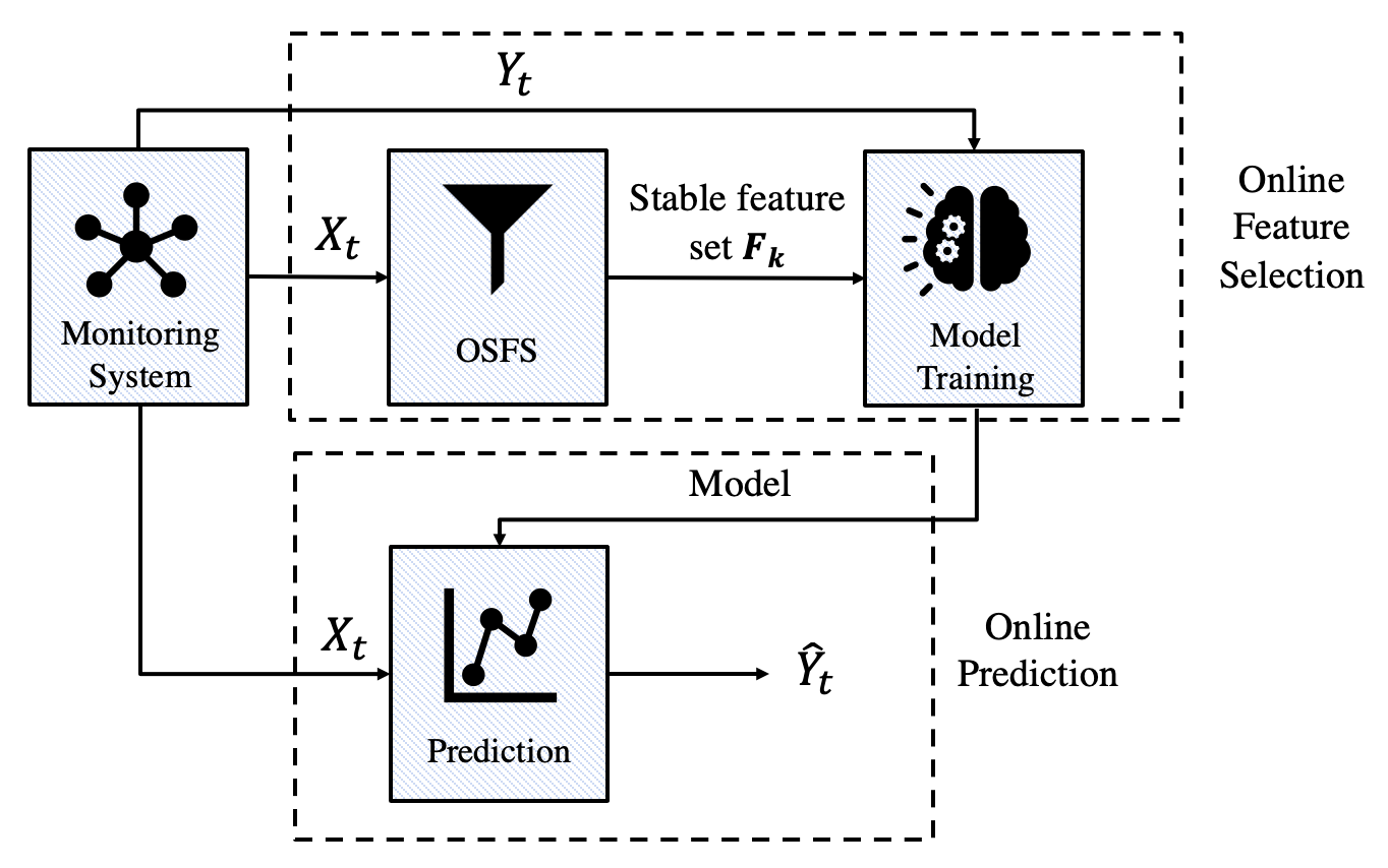
Figure 1: Online learning: feature selection and prediction. OSFS reads a stream of samples ($\emph{{X}}_{t}$) and extracts a stable feature set $\emph{{F}}_{k}$.

Our goal thus is to select $k$ and $t_{k}$ as small as possible, while enabling the models trained using $\emph{{F}}_{k}$ to be effective.

The task of selecting a subset of features from a larger set is called feature selection in machine learning and data mining and is a well-studied topic area. (See Section X). We are specifically interested in unsupervised feature selection methods, whereby the values of the target are not known during the feature selection process, i.e., the process to compute $\emph{{F}}_{k}$. This allows us to keep the feature selection process independent from the learning task and will enable different learning tasks in a system to share the same feature subset.

The specific problem we address in this paper is to design an online algorithm that reads a sequence of $n$-dimensional sample vectors $\emph{{X}}_{1},\emph{{X}}_{2},..$ one by one, computes $k$ and the feature set $\emph{{F}}_{k}$, and terminates after step $t_{k}$. The values for $k$ and $t_{k}$ must be small, while $\emph{{F}}_{k}$ must be equally effective as the feature set selected by the same ranking algorithm in an offline setting on the complete data stream. We measure the effectiveness of a feature set by computing the prediction error of the predictor trained with the feature set.

In our approach, we choose an unsupervised feature selection method that ranks the n features at every step $t$ of the online algorithm and checks how the top $i$ features ($i=1,..,n$) change with increasing $t$. We introduce two metrics to measure the stability of the feature set in Section IV. If the feature set of the top $k$ features has become sufficiently stable, the algorithm terminates and the values for $\emph{{F}}_{k}$, $k$ and $t_{k}$ are returned (see Section V).

Note that we assume here that the feature set F is fixed. In a real system that runs over some time, changes to the physical configuration or the virtualization layer occur, which result in changes to the set of available measurement points, i.e. the feature set. In such a case, the online algorithm must be re-started. Note also that we do not investigate how many samples are needed to train an accurate model for the learning task. This is left for future work.

III Creating ranked feature lists

In this section, we describe two algorithms (ARR, LS) that produce a ranked feature list from a list of samples. They are based on unsupervised feature selection methods from the literature. We will evaluate the suitability of these algorithms for our online feature selection method OSFS in Section V.

Table 1 shows the notation we use in the paper. The available data for computing the feature set $\emph{{F}}_{k}$ is presented as a design matrix $\emph{{X}}\in\mathbb{R}^{m\times n}$, whose $n$ columns represent the feature vectors and $m$ rows represent the samples in the data set. Since we assume that the samples arrive in sequence one-by-one, $m$ is increasing over time and can be interpreted as a time index.

TABLE 1: Table of notation

X	data set
$n$	number of features in X
$m$	number of samples in X
$\emph{{X}}_{i,:}\$or $\emph{{X}}_{i}(i=1,...,m)$	$i$-th row or $i$-th sample of X
$\emph{{X}}_{:,j}\ (j=1,...,n)$	$j$-th column or $j$-th feature vector of X
$\mathit{X_{i,j}}$	element of the $i$-th row and the $j$-th column of X
$k$	number of selected features
$t_{k}$	number of samples used for feature selection
F	set of all available features
$f_{j}\ (j=1,...,n)$	single feature in F
$\emph{{F}}_{k}$	subset with $k$ selected features
$\emph{{F}}_{k,t}$	the top $k$ features computed on $t$ samples

The first algorithm is Adapted Relevance Redundancy Feature Selection (ARR). It is based on the Relevance Redundancy Feature Selection (RRFS) method [3], which we adapted to compute a ranked feature list. ARR uses two criteria in assessing the rank of a feature: (a) relevance, which relates to the distance of a feature vector to the mean of all feature vectors, and (b) redundancy, which relates to the cosine similarity between a feature vector and the vectors of all other features. High relevance and low similarity result in a high score. The pseudo-code of ARR is given in Algorithm 1. First, the relevance of a feature is computed as the mean absolute difference of its feature vector from the mean (line 3). Then, the relevance of a feature is computed as the sum of the cosine similarity of its feature vector and each feature vector of the data set (lines 5-6). The score for ranking a feature is the relevance value divided by the redundancy value (line 7). The computational complexity of ARR is $O(n^{2}m)$. Recall that the cosine similarity between two features vectors $\emph{{X}}_{:,a}$ and $\emph{{X}}_{:,b}$ is calculated as:

$$cosim(\emph{{X}}_{:,a},\emph{{X}}_{:,b})=\left|\frac{\sum_{i=1}^{m}(\mathit{X_{i,a}}\mathit{X_{i,b}})}{(\sqrt{\sum_{i=1}^{m}\mathit{X_{i,a}}^{2}})(\sqrt{\sum_{i=1}^{m}\mathit{X_{i,b}}^{2}})}\right|$$ (1)

Input: Data matrix $\emph{{X}}\in\mathbb{R}^{m\times n}$

Output: Ranked feature list $\emph{{F}}^{{}^{\prime}}$

1 $\emph{{F}}^{{}^{\prime}}$=[];

2 for $i=1;i\leq n;i++$ do

3       $relevance_{i}=\sum_{j=1}^{m}\left|\mathit{X_{j,i}}-\overline{\emph{{X}}_{:,i}}\right|$;

4       $sim\_sum_{i}=0$;

5       for $j=1;j\leq n;j++$ do

6             $sim\_sum_{i}+=cosim(\emph{{X}}_{:,i},\emph{{X}}_{:,j})$;

7            

8      $score_{i}=\frac{relevance_{i}}{sim\_sum_{i}}$;

9      

10Construct $\emph{{F}}^{{}^{\prime}}$ as a list of all features sorted by $score_{i}$ in descending order;

11 return $\emph{{F}}^{{}^{\prime}}$;

Algorithm 1 Adapted Relevance Redundancy Feature Selection (ARR)

The second algorithm is Laplacian Score (LS) [4]. It follows the so-called filter method which examines intrinsic properties of the data to evaluate the features. LS ranks those features high that preserve locality with respect to a neighborhood graph. Algorithm 2 shows the pseudocode of LS. Input parameters for this algorithm are the design matrix and the number of local neighbors $K$. First, using the $m$ sample vectors as the nodes of the graph, a neighborhood graph is constructed with the $K$ nearest neighbors of each node as the links of the graph (line 1). Then, the graph connectivity and the distance between node pairs are used to compute the weight matrix (line 2). The graph Laplacian matrix is computed in line 4. The Laplacian score of all $n$ features is obtained in the for loop (lines 5-7). A low score for a feature signifies high locality preservation (see [4] for justification), and the features are ranked according to increasing score (line 8). The computational complexity of the LS algorithm is $O(nm^{2})$.

In the evaluations reported in Sections V and VI of this paper, we choose $K$ in relation to the value of $m$: $K=2$ for $0<m\leq 16$; $K=5$ for $16<m\leq 128$; $K=10$ for $m>128.$

Input: Data matrix $\emph{{X}}\in\mathbb{R}^{m\times n}$, $K\in\mathbb{N}$ nearest neighbors

Output: Ranked feature list $\emph{{F}}^{{}^{\prime}}$

1

2Construct graph G of $K$ nearest neighbors from nodes $\emph{{X}}_{i,:},i=1,..,m$;

3 Compute weight matrix $\emph{{S}}\in\mathbb{R}^{m\times m}$ from G

$$S_{ij}=\left\{\begin{matrix}e^{-\left\|\emph{{X}}_{i,:}-\emph{{X}}_{j,:}\right\|^{2}}&if\ nodes\ i\ and\ j\ are\ connected,\\ 0&otherwise\end{matrix}\right.$$

4 $\emph{{D}}=diag(\emph{{S1}})$ where $\emph{{1}}=\left[1,...,1\right]^{T}$, $\emph{{D}}\in\mathbb{R}^{m\times m}$;

5 $\emph{{L}}=\emph{{D}}-\emph{{S}}$;

6

7for $i=1;i\leq n;i++$ do

8       $\emph{{V}}_{i}=\emph{{X}}_{:,i}-\frac{\emph{{X}}_{:,i}^{T}\emph{{D}}\emph{{1}}}{\emph{{1}}^{T}\emph{{D}}\emph{{1}}}\emph{{1}}$ where $\emph{{V}}_{i}\in\mathbb{R}^{m\times 1}$;

9       $lscore_{i}=\frac{\emph{{V}}_{i}^{T}\emph{{L}}\emph{{V}}_{i}}{\emph{{V}}_{i}^{T}\emph{{D}}\emph{{V}}_{i}}$;

10      

11Construct $\emph{{F}}^{{}^{\prime}}$ as a list of all features sorted by $lscore_{i}$ in ascending order;

12 return $\emph{{F}}^{{}^{\prime}}$;

Algorithm 2 Laplacian Score (LS)

IV Computing stable feature sets

In Section III we discussed the algorithms ARR and LS, which produce ranked feature lists after reading $m$ samples $\emph{{X}}_{1}$, …, $\emph{{X}}_{m}$. In an online setting, where samples become available one-by-one at discrete times $t=1,2,...$, the value of $m$ can be interpreted as time. Let’s assume we run a feature ranking algorithm at time $t_{1}$ and compute the set $\emph{{F}}_{k,t_{1}}$ with the top $k$ features. This set will generally be different from the set $\emph{{F}}_{k,t_{2}}$ produced by the same algorithm at a later time $t_{2}$ for statistical reasons. Using the standard assumption from statistical learning that samples are drawn from static distributions [5], we expect that the sequence $\emph{{F}}_{k,t}$ converges to a set $\emph{{F*}}_{k}$ with increasing time $t$. Our objective for this section is to identify heuristic criteria that determine at which time the sequence $\emph{{F}}_{k,t},t=1,2,3,...$ has sufficiently converged or, as we also say, $\emph{{F}}_{k,t}$ has become “stable”.

We define two criteria for feature set stability, which use frequency-based stability methods [6]. The first is based on the similarity of two feature sets, the second on the variance of feature frequencies in feature sets.

IV-A A stability condition based on set similarity

Given two feature sets $\emph{{F}}_{k,t_{1}}$ and $\emph{{F}}_{k,t_{2}}$ ($k\in\mathbb{N}$), we define the similarity between them as the fraction of joint features:

$$sim(\emph{{F}}_{k,t_{1}},\emph{{F}}_{k,t_{2}}):=|\emph{{F}}_{k,t_{1}}\cap\emph{{F}}_{k,t_{2}}|/k$$ (2)

The values of the metric $sim$ lie between 0 and 1. $0$ means no similarity, i.e. $\emph{{F}}_{k,t_{1}}$ and $\emph{{F}}_{k,t_{2}}$ have no common features, while $1$ means the maximum similarity, i.e. $\emph{{F}}_{k,t_{1}}$ and $\emph{{F}}_{k,t_{2}}$ are identical.

When we study the evolution of $sim(\emph{{F}}_{k,t},\emph{{F}}_{k,2t})$ using the traces described in Section VII, we observe that the similarity metric tends to grow with the increase of $k$ and $t$. Also, this effect becomes stronger the larger $k$ and $t$ are. Figure 2 shows an example with data from the KTH testbed running a KV service.

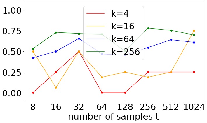
(a) $sim(\emph{{F}}_{k,t/2},\emph{{F}}_{k,t})$ vs $t$ in ARR

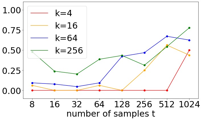
(b) $sim(\emph{{F}}_{k,t/2},\emph{{F}}_{k,t})$ vs $t$ in LS

Figure 2: The similarity of consecutive feature sets over time using ARR and LS with samples from the KV flash-crowd data set and start point $t=1$.

We introduce the first heuristic notion of a stable feature set:

$$\begin{split}\emph{{F}}_{k,t}\ is\ stable,\ iff\ sim(\emph{{F}}_{k,t},\emph{{F}}_{k,2t})>\eta\\ \ and\ sim(\emph{{F}}_{k,t},\emph{{F}}_{k,2t})>sim(\emph{{F}}_{k,2t},\emph{{F}}_{k,4t})\end{split}$$ (3)

Based on our experience with operational data, we set $\eta=0.5$ for this work. This means that $\emph{{F}}_{k,t}$ must share at least half of its features with $\emph{{F}}_{k,2t}$, which is computed with double the number of samples. The second condition in equation (3) is met if the sequence of similarity values reaches a local maximum. In Figure 2 (a) $\emph{{F}}_{64,32}$ and in Figure 2 (b) $\emph{{F}}_{64,512}$ are examples of stable feature sets.

IV-B A stability condition based on feature frequency

In [7] the authors propose a metric for feature set stability based on statistical concepts. They measure the selection frequency of each feature and estimate its variance for a sequence of consecutive feature sets. They model the frequency of a feature using a Bernoulli process. The stability criterion we introduce requires that the variance becomes sufficiently small.

Given a feature set $\emph{{F}}_{k,t}$ and the original feature set $\emph{{F}}=\left\{f_{1},f_{2},...,f_{n}\right\}$ ($k\in\mathbb{N},\ k\leq n$), we define the feature representation vector $\emph{{A}}_{k,t}\in\left\{0,1\right\}^{n}$ as follows

$$\emph{{A}}_{k,t}\left[j\right]=\left\{\begin{matrix}1,&if\ f_{j}\in\emph{{F}}_{k,t}\\ 0,&otherwise\end{matrix}\right.$$ (4)

We consider $r$ consecutive vectors and set the matrix $\emph{{Z}}_{k,t,r}:=[\emph{{A}}_{k,t},...,\emph{{A}}_{k,t+r-1}]^{T}$. We define the stability of $\emph{{F}}_{k,t}$ for $r$ consecutive feature sets as:

$$stab(\emph{{Z}}_{k,t,r}):=1-\frac{\frac{1}{n}\sum_{j=1}^{n}s_{j}^{2}}{\frac{k}{n}\left(1-\frac{k}{n}\right)}$$ (5)

To understand the right side of equation (5), we need to know that $p_{j}$ is the parameter of the Bernoulli process that models the occurrence of feature $f_{j}$. If we denote the empirical feature frequency with $\widehat{p_{j}}$, we can write $\widehat{p_{j}}=\frac{1}{r}\sum_{i=1}^{r}z_{ij}$ ($z_{ij}$ is an element of $\emph{{Z}}_{k,t,r}$). The empirical sample variance is given by $s_{j}^{2}=\frac{r}{r-1}\widehat{p_{j}}(1-\widehat{p_{j}})$. We know from theory that $s_{j}^{2}$ is an unbiased estimator of the variance of the feature frequency.

The stability metric $stab(\emph{{Z}}_{k,t,r})$ has values in $[-\frac{1}{r-1},1]$ [6]. If no feature shows any variance, i.e. each feature is either always selected or always left out, the value is 1. Otherwise, the value is less than 1.

Similar to $sim(\emph{{F}}_{k,t_{1}},\emph{{F}}_{k,t_{2}})$ we observe using the data from our testbed that $stab(\emph{{Z}}_{k,t,r})$ tends to grow with the increase of $k$ and $t$. This effect becomes stronger the larger $k$ and $t$ are. Figure 3 shows an example with data from the KTH testbed running a KV service.

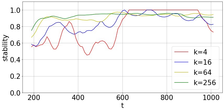
(a) $stab(\emph{{Z}}_{k,t,r})$ vs $t$ in ARR

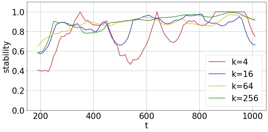
(b) $stab(\emph{{Z}}_{k,t,r})$ vs $t$ in LS

Figure 3: The feature set stability of current feature sets over time using ARR and LS with samples from the KV flash-crowd data set and start point $t=1$.

We introduce the second heuristic notion of a stable feature set:

$$\begin{split}\emph{{F}}_{k,t}\ is\ stable\ for\ r,\ iff\ stab(\emph{{Z}}_{k,t,r})>\eta\\ for\ w\ consecutive\ timesteps\end{split}$$ (6)

Based on our experience with operational data, we set $r=10$, $w=10$ and $\eta=0.9$ for this work. This means that when 10 consecutive stability values are all larger than 0.9, then the feature set $\emph{{F}}_{k,t}$ is stable. In Figure 3 (a) $\emph{{F}}_{4,600}$ and in Figure 3 (b) $\emph{{F}}_{4,840}$ are examples of stable feature sets.

IV-C Feature clustering

We also investigated a different approach to determine whether a feature set $\emph{{F}}_{k,t}$ is stable. This approach includes clustering the features after $t$ samples have been obtained. The two conditions we formulated to identify a stable feature set were then applied on the feature clusters instead of on individual features. The motivation for this approach stems from the idea that features in the same cluster have the same information content for constructing the prediction model. Specifically, we have used DBSCAN [8], which is based on the cosine similarity metric to cluster the features. However, the evaluation showed that the accuracy of the obtained predictors has been only marginally better than when clustering was not used. For this reason, we have not included the detailed results in this paper.

V OSFS: online feature selection with low overhead

In this section, we introduce the Online Stable Feature Set algorithm (OSFS), which reads a stream of samples $\emph{{X}}_{1}$, $\emph{{X}}_{2}$, $\emph{{X}}_{3}$,… and returns the number of features $k$, the number of samples $t_{k}$ needed to determine $k$, and the stable feature set $\emph{{F}}_{k,t_{k}}$.

Recall that the purpose of OSFS is to select a subset of available data sources (i.e. features), in order to reduce the monitoring costs and the training overhead for learning. To keep costs and overhead low, we want $k$ and $t_{k}$ to be small while still allowing for effective learning and prediction.

The standard use case for OSFS plays out as follows. We start monitoring the values of $n$ features at time $t=1$ and collect a sequence of samples with index $t=1,2,...$ We use the collected samples to find values for $k<<n$ and $t_{k}$ so that the first $t_{k}$ samples allow us to compute a stable feature set $\emph{{F}}_{k,t_{k}}$. At time $t_{k}+1$, we reduce the number of data sources from $n$ to $k$ and continue motoring only sources from the set $\emph{{F}}_{k,t_{k}}$.

We first present OSFS in a generic form, which allows for a range of instantiations and configurations. Algorithm 3 shows the options for configuration. First, we choose a feature ranking algorithm. Section III contains two examples of such algorithms, namely, ARR and LS. Second, we choose a condition for a feature set $\emph{{F}}_{k,t}$ to be stable. Section IV presents two possibilities of such conditions, namely, (3) and (6). Third, we choose the search space $S$, i.e. the space of possible values for $(k,t)$. An example of $S$ is a two-dimensional grid where $t$ has values $[16,64,256,1024]$ and $k$ has the values $[4,16,64,256]$. A search policy $P$ is an algorithm to traverse $S$. We have experimented with different search policies. For instance, policy $k-small$ starts with the smallest $k$, traverses all possible $t$ values, continues to the next larger $k$, traverses all possible $t$ values, etc. This way the grid is traversed from bottom to top (see Figure 4 red path). Similarly, the policy $t-small$ starts with the smallest $t$, traverses all possible $k$ values, continues to the next larger $t$, traverses all possible $k$ values, etc. This way the grid is traversed from left to right (see Figure 4 blue path). Many other policies are possible, for instance, random walk.

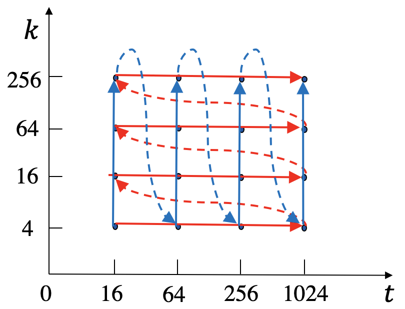
Figure 4: Search policy on one search space. The red path follows the policy $k-small$ and the blue path follows the policy $t-small$.

Once the execution of instantiated OSFS algorithm starts, initial values for $k$ and $t$ are selected (line 1). It then enters a loop where, during each iteration, one point in the grid is evaluated (line 2-7). First, the feature set $\emph{{F}}_{k,t}$ is computed using the ranking algorithm $A$ and available samples $\emph{{X}}_{1}$,…, $\emph{{X}}_{t}$. Then, the stability condition is evaluated for $\emph{{F}}_{k,t}$. If $\emph{{F}}_{k,t}$ is stable or the grid has been completely searched, the algorithm terminates and returns $\emph{{F}}_{k,t}$, $k$, $t$. Otherwise, the loop continues with the next $(k,t)$ pair.

When discussing the evaluations of OSFS in sections VIII and IX, we present results obtained with feature ranking algorithms ARR and LS and with both feature set stability conditions. Regarding the search policy, most of the results in this paper are obtained with $k-small$, which gives priority to a feature set of small size at the possible expense of larger running time of OSFS. We also perform evaluations with policy $t-small$, which prioritises obtaining a stable feature set within a short amount of time at the possible expense of a large feature set.

Input: Sample sequence $\emph{{X}}_{1}$, $\emph{{X}}_{2}$, $\emph{{X}}_{3}$,…;

         Feature ranking algorithm $A$;

         Metric and condition for stable feature set $C$;

         Search space $S$ for $(k,t)$;

         Search policy $P$ to traverse $S$.

Output: Stable feature subset $\emph{{F}}_{k,t}$, $k$, $t$.

1 Initialize $(k,t)$;

2 while True do

3       Compute $\emph{{F}}_{k,t}$ using $A$ on $\emph{{X}}_{1}$,…, $\emph{{X}}_{t}$;

4       if $\emph{{F}}_{k,t}$ is stable or $S$ is exhausted then

5             return $\emph{{F}}_{k,t}$, $k$, $t$;

6            

7      else

8             choose next $(k,t)$ following $P$;

9            

10      

Algorithm 3 Online Stable Feature Set (OSFS)

Input: Sample sequence $\emph{{X}}_{1}$, $\emph{{X}}_{2}$, $\emph{{X}}_{3}$,…;

         Feature ranking algorithm ARR;

         Metric $sim$ and condition (3) for stable feature

         set;

         Search space $[4-256]*[8-1024]$ for $(k,t)$;

         Search policy $k-small$.

Output: Feature subset $\emph{{F}}_{k,t_{k}}$, $k$, $t_{k}$

$subset(k,t,ARR)$ returns top $k$ features computed with ARR using samples with index $1,...,t$.

1 $\eta=0.5$ (threshold for stable feature set);

2 $read=false$;

3 for $k$ in [4,16,64,256] do

4       if $not\ read$ then

5             read and store $\emph{{X}}_{t},t=1,...,16$

6      $\emph{{F}}_{k1}=subset(k,8,ARR)$;

7       $\emph{{F}}_{k2}=subset(k,16,ARR)$;

8       $sim_{k12}=sim(\emph{{F}}_{k1},\emph{{F}}_{k2})$;

9      for $t=17,...,1024$ do

10             if $not\ read$ then

11                   read and store $\emph{{X}}_{t}$

12            if $t$ in [32,64,128,256,512,1024] then

13                  

14                  $\emph{{F}}_{kt}=subset(k,t,ARR)$;

15                   $sim_{kt}=sim(\emph{{F}}_{k2},\emph{{F}}_{kt})$;

16                   if $sim_{kt}<sim_{k12}\ and\ sim_{k12}>\eta$ then

17                         return $\emph{{F}}_{k1},k,t/4$;

18                        

19                  else if $sim_{kt}>\eta\ and\ t==1024$ then

20                         return $\emph{{F}}_{k2},k,t/2$;

21                        

22                  else

23                         $\emph{{F}}_{k1}=\emph{{F}}_{k2}$;

24                         $\emph{{F}}_{k2}=\emph{{F}}_{kt}$;

25                         $sim_{k12}=sim_{kt}$;

26                  

27            

28      $read=true$

return $\emph{{F}}_{k2},256,1024$

Algorithm 4 OSFS-ARR-$sim$-$k-small$

Algorithm 4 is an example of an instantiated OSFS algorithm, which we use for evaluation. The algorithm takes as input the sequence of arriving samples $\emph{{X}}_{t}$ and is initialized with the feature ranking algorithm ARR. ARR is used in the function $subset()$, which takes as input $k$ and the first $t$ samples and returns a set with the top $k$ features ranked by ARR.

It has two main loops: an outer loop (lines 3-23) that iterates over a subspace of $k$ and an inner loop (lines 9-22) that iterates over a subspace of $t$. The index values of $k$ and $t$ increase exponentially to enable the exploration of a large space with a small number of evaluations. The algorithm performs a grid search in the space of tuples $(k,t)$ with the termination condition A: $sim_{kt}<sim_{k12}\ and\ sim_{k12}>\eta$ (line 15) or B: $sim_{kt}>\eta\ and\ t==1024$ (line 17). In case the conditions A or B are never met, the algorithm terminates after the search on the grid sector $[4-256]*[8-1024]$ has been completed. The key termination condition A expresses the case where (1) the similarity of two consecutive feature sets is above the threshold $\eta$ and (2) the similarity declines when the subsequent feature set is considered.

The algorithm reads at least 32 samples in order to ensure statistical viability and terminates after at most 1024 samples. Since the outer loop is indexed by increasing $k$, it favors a smaller $k$ at the possible expense of a larger $t$. This means that we prefer reducing the monitoring overhead over reducing the time to compute $\emph{{F}}_{k,t}$.

VI Recomputing feature set after concept drift

The distribution from which the samples are drawn for training prediction models can evolve over time, and this phenomenon is referred to as concept drift, which is a well-studied topic in data analysis [9]. When concept drift occurs, the prediction model must generally be recomputed in order to maintain prediction accuracy. In addition, the feature set from which the prediction model is computed should be adapted as well for the same reason.

In the context of network systems and their operation, concept drift can occur when a system is reconfigured or when the resource allocation policy for services or applications is changed. This means that, when concept drift occurs, OSFS must be run again to identify the updated set of features for recomputing the prediction model.

In this work, we use a state-of-the-art concept drift detection algorithm called STUDD (Student-Teacher Method for Unsupervised Concept Drift Detection) [10] on our data traces. STUDD detects concept drift in an unsupervised manner by using a student-teacher paradigm [11]. The basic idea of this paradigm is that in addition to the primary predictor, which is called teacher, a second predictor, which is called student, is trained. The student model is learned on the same input dataset X as the teacher, but the target set Y is replaced with the values predicted by the teacher. During the prediction phase, the discrepancy between the teacher’s prediction and the student’s prediction for the same target values is monitored. The Page-Hinkley test [12] is applied to detect changes in the time series of the discrepancy values. Such a change indicates a concept drift event.

We use a random forest regressor to compute the teacher as well as the student models.

In Section IX we study the effect of recomputing the stable feature set on the prediction accuracy using the KTH dataset. Specifically, we compare the accuracy values for scenarios where the stable feature set is recomputed after change detection, with scenarios where the stable feature set is computed only at the beginning of the trace.

VII Traces for evaluation

VII-A KTH testbed traces

Figure 5 outlines our laboratory testbed at KTH. It includes a server cluster, an emulated OpenFlow network, and a set of clients. A more detailed description of the KTH testbed setup and the services running on it is given in [13].

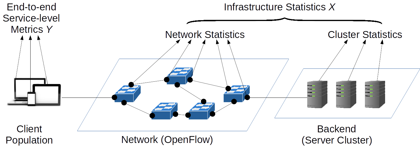
Figure 5: The testbed at KTH, providing the infrastructure for experiments. In various scenarios we predict end-to-end service-level metrics from low-level infrastructure measurements [13].

The online feature selection method proposed in this paper has been evaluated using data from four experiments. Two of them involve running a Video-on-Demand (VoD) service and two a Key Value store (KV) service.

1. VoD periodic: In this experiment, we run the VoD service under a periodic load pattern on the testbed. Data is collected every second over a period of $50\,000$ seconds. After cleaning the dataset, it contains $50\,000$ samples and $1\,296$ features. More details about the experiment are given in [14].

2. VoD flash-crowd: This experiment relies on the same setup as VoD periodic, except that the testbed is loaded with a flash-crowd pattern. After cleaning the dataset, $50\,000$ samples and $1\,255$ features remain. More details about the experiment are given in [14].

3. KV periodic: In this experiment, we run the KV service under a periodic load pattern on the testbed. Measurements are collected every second over a period of $28\,962$ seconds. The dataset contains $10\,374$ features collected from the server cluster and $176$ features from the network switches. After cleaning the data set, $1\,751$ features remain. More details about the experiment are given in [13].

4. KV flash-crowd: This experiment relies on the same setup as KV periodic, except that the testbed is loaded with a flash-crowd pattern. After cleaning the dataset, $19\,444$ samples and $1\,723$ features remain. More details about the experiment are given in [13].

Table 2 summarizes the basic information of these four traces. All four traces are available at [15].

TABLE 2: Datasets from KTH test bed

Dataset	Number of features	Number of samples	Target
KV flash crowd	1723	19444	${}^{\prime}ReadsAvg^{\prime}$
KV periodic	1751	28962	${}^{\prime}ReadsAvg^{\prime}$
VoD flash crowd	1255	50000	${}^{\prime}DispFrames^{\prime}$
VoD periodic	1296	50000	${}^{\prime}DispFrames^{\prime}$

VII-B FedCSIS 2020 Challenge dataset

The FedCSIS 2020 Challenge dataset [1] is a public dataset provided by EMCA Software, an analytics company. It contains around 2000 samples collected from December 2019 to February 2020. Each sample aggregates one hour of measurements, and there are 24 samples per day. The data are gathered from 3728 hosts. Hosts can have different numbers of attributes. For each attribute, such as CPU utilization, several feature columns are included, for example, the mean value, the standard deviation. From the challenge dataset, we construct two smaller datasets for evaluation. In each of these two datasets, all samples share the same features.

• Dataset1 contains samples from hosts that have the following six attributes $[^{\prime}cpu\_1m^{\prime},^{\prime}cpu\_5m^{\prime},^{\prime}cpu\_5s^{\prime},^{\prime}memoory\_free^{\prime},$ ${}^{\prime}memory\_total^{\prime},^{\prime}memory\_used^{\prime}]$. For every attribute, four feature columns are included with the mean, the standard deviation, the minimum and the maximum value, respectively.

• Dataset2 contains samples from hosts that have the following six attributes $[^{\prime}cpuusagebyproc^{\prime},^{\prime}memoryallocatedbyproc^{\prime},$ ${}^{\prime}in\_traffic^{\prime},^{\prime}out\_traffic^{\prime},^{\prime}error\_in^{\prime},^{\prime}error\_out^{\prime}]$. For every attribute, four feature columns are included with the mean, the standard deviation, the minimum and the maximum value, respectively.

In these two datasets, many feature values are missing. We remove all feature columns where more than 30% of the values are missing. The remaining missing values are estimated through linear interpolation. After these steps, the number of features and the number of samples in each dataset are listed in Table 3.

TABLE 3: Datasets from FedCSIS 2020 Challenge dataset

Dataset	Number of features	Number of samples
Dataset1	30438	1917
Dataset2	10163	1917

VIII Evaluation of OSFS on different data sets

We evaluate OSFS by asking two main questions:

1. How effective is OSFS in reducing communication and computing overhead as well as the data collection time, i.e. the number of samples needed for feature selection? What are typical values for $k$ and $t_{k}$ for the KTH and FedCSIS datasets?

2. How effective is OSFS in producing feature sets for training accurate prediction models?

To obtain the evaluation results, we perform two preprocessing steps on the datasets. First, we linearly scale the values of each feature vector to the range $[0,1]$. Second, we remove the feature vectors with a variance below 0.0001. For prediction, we use a random forest regressor from the scikit-learn library [16]. As for hyperparameters, we use 100 trees and the default values for the other parameters. The prediction error is expressed as Normalized Mean Absolute Error (NMAE), which is computed as follows:

$$NMAE(\widehat{y_{1}},...,\widehat{y_{q}})=\frac{1}{\overline{y}}(\frac{1}{q}\sum_{i=1}^{q}\left|y_{i}-\widehat{y_{i}}\right|)$$ (7)

where $\overline{y}$ is the mean value of targets in the test set, $q$ is the number of samples and $\widehat{y_{i}}$ is the predicted value.

Table 4 shows the evaluations for the KTH datasets and Table 5 for the FedCSIS datasets. Both tables have the same column structure. The first column identifies the dataset, the second column lists the feature ranking algorithm, the third column gives the feature set stability metric, the fourth column gives the search policy. The fifth and sixth columns give the output of OSFS, the seventh and eighth columns provide the prediction error.

Each row in Tables 4 and 5 shows the result from an evaluation scenario for a given dataset, feature ranking algorithm, feature set stability metric and search policy. A scenario contains ten evaluation runs of OSFS with different start points on the dataset (whereby one start point is t=1 and the other 9 are chosen uniformly at random between t=2 and t=10 000).

We observe that OSFS produces a range of feature set sizes $k$, from 4 to 212. The same applies to the number of samples $t_{k}$ (i.e. the data collection time) with a range from 8 to 882. As expected, the search policy $k-small$ produces small values for $k$ and larger values for $t_{k}$, and for the search policy $t-small$, the opposite applies. In all scenarios, we see a significant reduction of the size of the feature sets compared with the total number of features. We also find that, while the values for $k$ and $t_{k}$ are strongly dependent on the search policy, they are less influenced by other parameters, namely, the type of dataset and the feature ranking algorithm.

The column Online FS error shows the error of a prediction model trained with the feature set of size $k$ that has been produced with $t_{k}$ samples. These values reflect the capability of OSFS to produce an effective feature set for model training. We compare the results with two baseline methods. The first baseline method uses all samples of the dataset for feature selection. The values for this baseline are listed in column Offline FS error. The second baseline method does not rely on feature selection and uses all features to train the prediction model. The result for this method is listed in the lowest row of each dataset and indicated by No FS.

Comparing the values in column Offline FS error with the error values in No FS shows us the cost of reducing the feature set. Depending on the scenario, the difference in error ranges from 2% to 115% for the KTH datasets and from 158% to 369% for the FedCSIS datasets. (We explain the larger difference on the FedCSIS datasets with the fact that the complete feature space of the FedCSIS datasets is between 5 and 16 times larger than that of the KTH datasets, while the number of selected features by OSFS is almost the same.) While the difference in the error can be quite significant, we have shown in earlier research that it can be effectively reduced by using a supervised feature ranking algorithm instead of an unsupervised one [17].

Most importantly, the values in the column Online FS error tend to be somewhat smaller than those in Offline FS error, 6% on KTH datasets and 25% on FedCSIS datasets in average. This result suggests that OSFS is effective as an online feature selection algorithm and is robust regarding the sample interval on the trace that is used for feature selection.

TABLE 4: Evaluation of OSFS on KTH data sets. The prediction method is random forest. The error is expressed in NMAE (7). Each row shows the result from an evaluation scenario with ten runs.

Dataset	Method	Metric	Search	$k$	$t_{k}$	Online FS error	Offline FS error
KV flash-crowd	ARR	Similarity	$k-small$	$25.6\pm 25.6$	$251.2\pm 224.0$	$\textbf{0.0280}\pm 0.0056$	$0.0304\pm 0.0049$
		Stability	$k-small$	$17.2\pm 16.5$	$744\pm 159.6$	$\textbf{0.0299}\pm 0.0054$	$0.0322\pm 0.0033$
			$t-small$	$192.4\pm 98.4$	$472\pm 56.9$	$\textbf{0.0233}\pm 0.0060$	$0.0227\pm 0.0043$
	LS	Similarity	$k-small$	$10\pm 6$	$64\pm 72.3$	$\textbf{0.0232}\pm 0.0014$	$0.0255\pm 0.0007$
		Stability	$k-small$	$6.4\pm 4.8$	$724\pm 244.7$	$\textbf{0.0289}\pm 0.0054$	$0.0322\pm 0.0037$
			$t-small$	$186.4\pm 107.4$	$472\pm 83$	$\textbf{0.0235}\pm 0.0060$	$0.0234\pm 0.0054$
	No FS			1723			0.0184
KV periodic	ARR	Similarity	$k-small$	$10\pm 6$	$249.6\pm 194.4$	$\textbf{0.0325}\pm 0.0071$	$0.0434\pm 0.0006$
		Stability	$k-small$	$8.8\pm 5.9$	$660\pm 179.5$	$\textbf{0.0294}\pm 0.0015$	$0.0435\pm 0.0006$
			$t-small$	$211.6\pm 89.8$	$415\pm 50.2$	$\textbf{0.0253}\pm 0.0011$	$0.0263\pm 0.0059$
	LS	Similarity	$k-small$	$12.4\pm 5.5$	$195.2\pm 177.3$	$\textbf{0.0268}\pm 0.0016$	$0.0264\pm 0.0001$
		Stability	$k-small$	$14.8\pm 17.3$	$514\pm 180.5$	$\textbf{0.0273}\pm 0.0014$	$0.0262\pm 0.0005$
			$t-small$	$122.8\pm 111.2$	$451\pm 68.3$	$\textbf{0.0245}\pm 0.0025$	$0.0249\pm 0.0010$
	No FS			1751			0.0214
VoD flash-crowd	ARR	Similarity	$k-small$	$12.4\pm 5.5$	$131.2\pm 142.7$	$\textbf{0.1629}\pm 0.0139$	$0.1328\pm 0.0083$
		Stability	$k-small$	$16\pm 17.0$	$724\pm 198.1$	$\textbf{0.1340}\pm 0.0067$	$0.1349\pm 0.0087$
			$t-small$	$140.8\pm 94.1$	$387\pm 74.6$	$\textbf{0.1081}\pm 0.0255$	$0.1129\pm 0.0222$
	LS	Similarity	$k-small$	$17.2\pm 16.5$	$226.4\pm 198.2$	$\textbf{0.0969}\pm 0.0405$	$0.1469\pm 0.0257$
		Stability	$k-small$	$7.6\pm 5.5$	$749\pm 213.2$	$\textbf{0.1170}\pm 0.0338$	$0.1657\pm 0.0135$
			$t-small$	$167.2\pm 110.4$	$520\pm 85.2$	$\textbf{0.0817}\pm 0.0320$	$0.0899\pm 0.0425$
	No FS			1255			0.0771
VoD periodic	ARR	Similarity	$k-small$	$10\pm 6$	$363.2\pm 196.5$	$\textbf{0.2085}\pm 0.0203$	$0.1795\pm 0.0041$
		Stability	$k-small$	$5.2\pm 3.6$	$781\pm 168.2$	$\textbf{0.2123}\pm 0.0189$	$0.1827\pm 0.0024$
			$t-small$	$174.4\pm 100.8$	$356\pm 59.2$	$\textbf{0.1413}\pm 0.0196$	$0.1384\pm 0.0259$
	LS	Similarity	$k-small$	$25.6\pm 25.6$	$108\pm 85.5$	$\textbf{0.1162}\pm 0.0295$	$0.1426\pm 0.0718$
		Stability	$k-small$	$17.2\pm 16.5$	$686\pm 145.9$	$\textbf{0.1139}\pm 0.0605$	$0.1166\pm 0.0739$
			$t-small$	$211.6\pm 89.8$	$541\pm 115.7$	$\textbf{0.1130}\pm 0.0084$	$0.1243\pm 0.0344$
	No FS			1296			0.1190

TABLE 5: Evaluation of OSFS on FedCSIS 2020 Challenge data sets. The prediction method is random forest. The error is expressed in NMAE (7). Each row shows the result from an evaluation scenario with ten runs. For dataset1, the prediction target is ${}^{\prime}host4846\_cpuusagebyproc\_mean^{\prime}$ and for dataset2 is ${}^{\prime}host0958\_cpu\_1m\_mean^{\prime}$.

Dataset	Method	Metric	Search	$k$	$t_{k}$	Online FS error	Offline FS error
Dataset1	ARR	Similarity	$k-small$	$26.8\pm 24.9$	$217.6\pm 169.2$	$\textbf{0.701}\pm 0.124$	$0.593\pm 0.243$
		Stability	$k-small$	$10\pm 6$	$600\pm 135.2$	$\textbf{0.829}\pm 0.132$	$0.730\pm 0.218$
	LS	Similarity	$k-small$	$10\pm 18$	$8\pm 0$	$\textbf{0.291}\pm 0.024$	$0.884\pm 0.170$
		Stability	$k-small$	$44.8\pm 73.8$	$876\pm 66.7$	$\textbf{0.569}\pm 0.197$	$0.715\pm 0.249$
	No FS			10162			0.230
Dataset2	ARR	Similarity	$k-small$	$168.4\pm 108.7$	$153.6\pm 145.1$	$\textbf{0.221}\pm 0.128$	$0.208\pm 0.103$
		Stability	$k-small$	$42.4\pm 26.7$	$882\pm 65.2$	$\textbf{0.275}\pm 0.121$	$0.272\pm 0.116$
	LS	Similarity	$k-small$	$4\pm 0$	$92.8\pm 36.3$	$\textbf{0.055}\pm 0.004$	$0.218\pm 0$
		Stability	$k-small$	$4\pm 0$	$337\pm 69.7$	$\textbf{0.055}\pm 0.003$	$0.218\pm 0$
	No FS			30437			0.058

Other conclusions we draw from Tables 4 and 5:

• OSFS can achieve a massive reduction in the size of the feature set, 1-3 orders of magnitude.

• The number of samples needed to compute the feature sets averages around 430 on the investigated datasets. For the KTH testbed, where metrics are monitored once per second, this means that OSFS produces a stable feature set within an average of 7 minutes.

• The feature ranking algorithm LS generally provides much better results than ARR, although at the cost of higher computational complexity when the number of samples used for feature selection becomes large (see Section III).

• Consistent with our earlier results (e.g., [18, 13]), we find that the type of service and the load pattern significantly affect the prediction error.

• We find that neither the feature set similarity metric nor the feature set stability metric outperforms the other on the datasets we investigated. Since the feature set similarity has a lower computational complexity, we prefer this metric for future investigations.

• On the investigated datasets, OSFS achieves the best results, on average, with feature ranking algorithm LS, search policy $k-small$, and the feature set similarity metric.

IX Evaluation of OSFS with online training and change detection

In Section VIII, we evaluate OSFS by studying the prediction error of a random forest regressor. In this case, feature selection is performed online, but model training of the regressor is performed offline. The column Online FS error in Tables 4 and 5 gives the evaluation results.

Building on these results, we investigate two key questions in this section. First, which prediction accuracy can be achieved when not only feature selection is performed online, but also model training, and how do the results compare to offline training? Second, can better prediction accuracy be achieved if the feature set is adapted over time? We address the second question through detecting concept drift, i.e. a change in the conditional distribution $P(Y|X)$ over time (see Section X). We use the STUDD algorithm for the concept drift detection (see Section VI).

The implementation of the Page-Hinkley test in STUDD uses the scikit-multiflow library [19] with the change parameter $delta$ set to 0.05. Regarding OSFS, we use the $k-small$ search policy and the $similarity$ metric.

Table 6 summarizes the results of these evaluations. The first column indicates the dataset, the second shows the feature ranking algorithm, the third column (Offline train) gives the prediction error when using online feature selection and offline training. (The values are computed the same way as in Table 4 column Online FS error.) The fourth column (Online train) shows the prediction error when using online feature selection and online training. The fifth column (Model retrain) gives the results when using online feature selection, online training and model re-training after concept drift is detected. The sixth column (Model retrain and feature recomp) provides the most important results. It shows the prediction error when using online feature selection, online learning as well as feature set re-computation and model re-training after detecting concept drift. Finally, the last column (change) indicates the number of changes in concepts discovered on the trace.

Each row in Table 6 lists the result from a run with start point $t=1$. Figure 6 describes how an experiment takes place. At the start point $t_{0}$, the system begins with periodically collecting samples with values from the entire feature set F. At time $t_{0}^{{}^{\prime}}$, OSFS returns a stable feature set $\emph{{F}}_{0}$ (based on the samples in the interval [$t_{0}$,$t_{0}^{{}^{\prime}}$]). At this point, the monitoring system begins to collect samples with values only from the reduced feature set $\emph{{F}}_{0}$. Based on this feature set, the prediction model $M_{0}$ is trained and the system starts predicting target values. In the case of online training, the samples in the interval [$t_{0}$,$t_{0}^{{}^{\prime}}$] are used. At time $t_{1}$, the change detection algorithm detects a concept drift and triggers OSFS to recompute the feature set. At this point, the monitoring system switches to monitor the values from the entire feature set F. The newly computed feature set $\emph{{F}}_{1}$ becomes available at time $t_{1}^{{}^{\prime}}$. In the case of model re-training, the new predictor $M_{1}$ is trained with the samples from the interval [$t_{1}$,$t_{1}^{{}^{\prime}}$]. For reason of simplicity, the training time is omitted in Figure 6.

From Table 6, we gain the following insights regarding the performance of OSFS on the studied datasets:

• Feature set re-computation is effective as it can achieve a reduction in error by 3% to 6%, in addition to the reduction achieved by model re-training (8% to 80%).

• Online training (Online train), compared with offline training (Offline train), incurs 18% to 955% higher prediction error. This error can be reduced by considering additional samples for training. Note that decreasing the difference in prediction error between online training and offline training is not studied in this work, as the focus is on online feature selection.

In summary, the error of a predictor can be significantly reduced by recomputing the feature set and retraining the model after a concept drift.

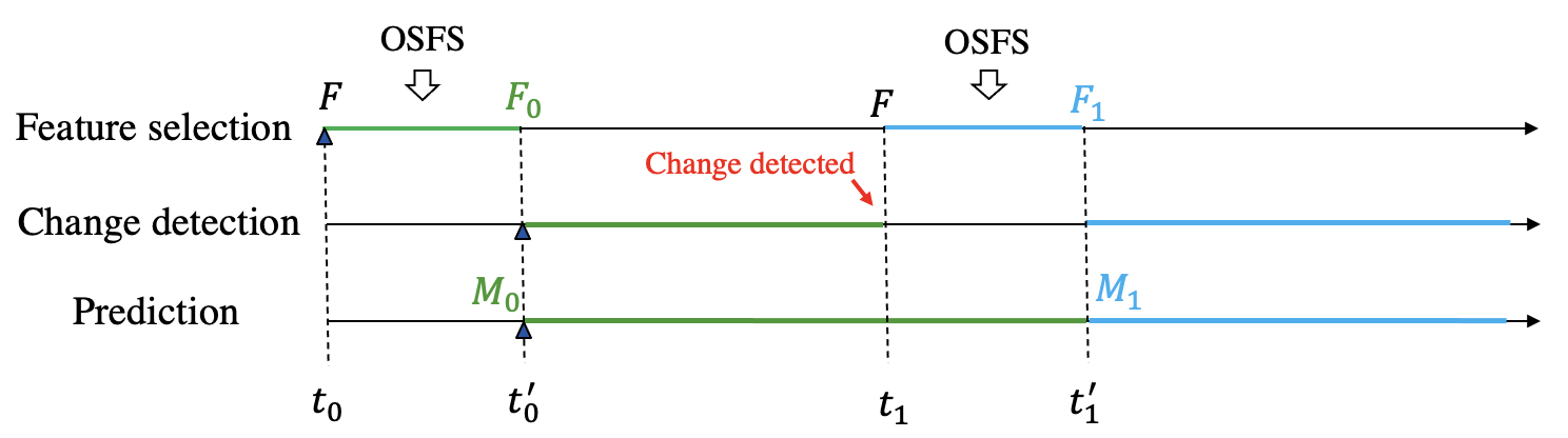
Figure 6: OSFS selects subset $F_{0}$ from the entire feature set $F$ using samples from interval [$t_{0}$,$t_{0}^{{}^{\prime}}$]. When a change is detected at time $t_{1}$, OSFS selects subset $F_{1}$ from $F$ using samples from interval [$t_{1}$,$t_{1}^{{}^{\prime}}$].

TABLE 6: Evaluation of OSFS for online model training and model re-training under change detection. The prediction method is random forest. The error is expressed in NMAE (7). The most important column is ’Model retrain and feature recomp’, which shows he prediction error when using online feature selection, online learning as well as feature set re-compuation and model re-training after detecting concept drift.

Dataset	Method	Offline train	Online train	Model retrain	Model retrain and feature recomp	change
KV flash-crowd	ARR	0.0238	0.0387	0.0387	0.0387	0
	LS	0.0232	0.2447	0.0389	0.0393	1
KV periodic	ARR	0.0436	0.1554	0.0579	0.0531	2
	LS	0.0261	0.0985	0.0588	0.0534	2
VoD flash-crowd	ARR	0.1499	0.1163	0.1163	0.1163	0
	LS	0.0654	0.1157	0.1157	0.1157	0
VoD periodic	ARR	0.2280	0.2700	0.1789	0.1789	1
	LS	0.1844	0.1840	0.1687	0.1684	1

X Related work

In the context of this paper, we understand online learning as an iterative learning method where training samples arrive sequentially as a data stream. Periodic monitoring of infrastructure metrics in a networked system creates such a stream of samples. The learning algorithms that enable learning on a stream of samples are often referred to as incremental learning. [20] formalizes the concept of incremental learning and discusses algorithms that require only constant memory. In [21], the authors compare eight incremental learning algorithms for supervised classification. Instead of the term incremental learning, many authors use the expression learning on data streams. [22] is a textbook that provides a state-of-the-art description of this subject. Algorithms for data stream mining including classification, regression, clustering, and frequent pattern mining are discussed. Most of these algorithms are adapted from well-known offline learning algorithms.

Most works that address learning on data streams assume that the samples in a data stream are drawn from a distribution $P(X,Y)$, which is also referred to as a concept [23]. The change of such a concept is called a concept drift. For our research, it is important to detect a change in the conditional distribution $P(Y|X)$, which is called a real concept drift [23]. In this paper, we use the STUDD algorithm [10] for detecting a change in the conditional probability distribution $P(Y|X)$ (see Section VI). [9] provides a survey on concept drift adaptation methods, which detect concept drift and adapt the prediction model. The paper contains a taxonomy of such methods. It also lists metrics for the evaluation of change detection methods.

A key challenge in learning on operational data from networked systems, which are distributed by nature, is respecting the resource constraints. The extraction of data on the devices, their transportation, the data preprocessing, and the model training require network, computing and memory resources. Much research has been conducted to reduce resource consumption while still being able to produce accurate prediction models. One research direction is online sample selection where samples are kept in a cache of constant size for later processing and model training. A sample selection algorithm decides which samples should be stored in the cache and which should be dropped from the data stream. A well-known and efficient algorithm is reservoir sampling, which chooses a sample set of fixed size uniformly at random from a population of unknown size in a single pass [24]. In earlier work [25] we have evaluated four online sampling algorithms which have been derived from known algorithms. We specifically argue that feature selection algorithms can be adapted for sample selection and provide experimental evidence that the resulting algorithms can be effective.

A second research direction focuses on reducing the dimensionality of the feature space, which corresponds to the number of features. Many methods have been developed that map a high-dimensional feature space into a low-dimensional space. Principal Components Analysis (PCA) [26] is a linear and popular method that is often used for this purpose. A second method, which is based on neural networks, is auto-encoder [26]. Another approach to reduce the dimensionality of the feature space is feature selection. In this paper, we study feature selection methods, because they allow us to significantly reduce monitoring costs, in addition to saving model training costs. The other dimensionality reduction methods described above only reduce model training costs.

Feature selection has been studied as an effective data preprocessing strategy in both the machine learning and data mining fields for several decades. Many survey papers cover and compare feature selection methods, e.g. [27][28][29][30][31]. For instance, [29] provides a useful categorization of feature selection methods along several dimensions, such as supervised and unsupervised methods; wrapper, filter, and embedded methods; and static or streaming methods. In [31], the authors evaluate several supervised feature selection methods on security datasets. They investigate the prediction performance and computing time of these algorithms. They find that the selected feature set varies with the type of attack recorded in the dataset.

Most feature selection methods described in the literature have been developed for offline learning where all data fits into memory. In recent years however, online feature selection methods have received increasing attention. In this case, the input to the algorithm is either a stream of feature vectors (e.g. [32][33][34][35][36][37]) or a stream of samples (e.g. [38][39][37]). Interestingly, most published online feature selection methods fall into the first category and process a stream of feature vectors. Such methods are not suitable for the problem we study in this paper, since, in our case, the data becomes gradually available as time progresses. Our interest thus is in methods that process streams of samples. Examples of such works are [38], [39], and [37].

In [38], the authors perform online supervised feature selection as a part of training the perceptron algorithm. During a training step, the values of the selected features are used to update the weights of the perceptron. Features with large weights are selected with high probability and features with small weights are selected with low probability. More closely related to our work is [39], which presents an unsupervised online feature selection algorithm based on clustering. The algorithm uses constant memory. In [37], the authors introduce an online feature selection algorithm called Geometric Online Adaption (GOA). A characteristic of this algorithm is that it works for both streams of samples and streams of feature vectors.

Note that a large part of the online feature selection algorithms we found in the literature require the number of features to be selected as an input parameter. The algorithm we present in this paper attempts to find a small but sufficiently large number of features that form a stable feature set.

The authors of [40] provide a recent survey of work on the stability of feature selection algorithms. By stability, they mean that an algorithm selects similar feature sets from similar sample sets. Another survey is given in [6], which additionally proposes a novel metric for measuring feature set stability. We are using this metric in Section IV.

XI Conclusions and future work

In this paper, we introduced OSFS, an online algorithm that selects a small set from a large number of available data sources, which allows for rapid, low-overhead learning and prediction. OSFS is instantiated with a set of options and performs a grid search that terminates when a stable feature set has been identified.

For all traces investigated, we found that OSFS achieves a massive reduction in the size of the feature set while maintaining its performance for training predictors. We have shown the effectiveness of OSFS as an online feature selection algorithm which is robust regarding the sample interval used for feature selection. In addition, we found that, if concept drift occurs, its effect can be mitigated by recomputing the feature set with OSFS and retraining the prediction model.

Regarding future work, there are many ways our method can be improved or extended. We can evaluate OSFS with additional instantiations of feature ranking algorithms, stability conditions, and search policies. Also, the tradeoffs between the three metrics $k$, $t_{k}$, and the prediction error warrant further study.

Online learning is only one part of efficiently producing a learning model using online techniques. Other parts include online sample selection [25], and the integration of online feature selection, online sample selection and online training into a joint framework. Finally, we believe it should be investigated how such a framework can be distributed, since we envision both training and prediction as distributed processes in future networked systems.

XII Acknowledgements

The authors are grateful to Andreas Johnsson, Hannes Larsson, and Jalil Taghia with Ericsson Research for fruitful discussion around this work, as well as to Forough Shahab Samani, Kim Hammar, and Rodolfo Villaça for comments on an earlier version of this paper. This research has been partially supported by the Swedish Governmental Agency for Innovation Systems, VINNOVA, through project AutoDC, and by Digital Futures through project Democritus.

References

- [1] A. Janusz, M. Przyborowski, P. Biczyk, and D. Ślęzak, “Network device workload prediction: A data mining challenge at knowledge pit,” in 2020 15th Conference on Computer Science and Information Systems (FedCSIS). IEEE, 2020, pp. 77–80.
- [2] X. Wang, F. S. Samani, and R. Stadler, “Online feature selection for rapid, low-overhead learning in networked systems,” in 2020 16th International Conference on Network and Service Management (CNSM). IEEE, 2020, pp. 1–7.
- [3] A. J. Ferreira and M. A. Figueiredo, “An unsupervised approach to feature discretization and selection,” Pattern Recognition, vol. 45, no. 9, pp. 3048–3060, 2012.
- [4] X. He, D. Cai, and P. Niyogi, “Laplacian score for feature selection,” in Advances in neural information processing systems, 2006, pp. 507–514.
- [5] V. N. Vapnik, Statistical learning theory. John Wiley, 1998.
- [6] S. Nogueira, K. Sechidis, and G. Brown, “On the stability of feature selection algorithms.” J. Mach. Learn. Res., vol. 18, no. 1, pp. 6345–6398, 2017.
- [7] J. Haug, M. Pawelczyk, K. Broelemann, and G. Kasneci, “Leveraging model inherent variable importance for stable online feature selection,” in Proceedings of the 26th ACM SIGKDD International Conference on Knowledge Discovery & Data Mining, 2020, pp. 1478–1502.
- [8] scikit-learn developers, “Dbscan,” 2007-2019. [Online]. Available: https://scikit-learn.org/stable/modules/generated/sklearn.cluster.DBSCAN.html
- [9] J. Gama, I. Žliobaitė, A. Bifet, M. Pechenizkiy, and A. Bouchachia, “A survey on concept drift adaptation,” ACM computing surveys (CSUR), vol. 46, no. 4, pp. 1–37, 2014.
- [10] V. Cerqueira, H. M. Gomes, A. Bifet, and L. Torgo, “Studd: A student-teacher method for unsupervised concept drift detection,” arXiv preprint arXiv:2103.00903, 2021.
- [11] C. Bucilua, R. Caruana, and A. Niculescu-Mizil, “Model compression,” in Proceedings of the 12th ACM SIGKDD international conference on Knowledge discovery and data mining, 2006, pp. 535–541.
- [12] E. S. Page, “Continuous inspection schemes,” Biometrika, vol. 41, no. 1/2, pp. 100–115, 1954.
- [13] R. Stadler, R. Pasquini, and V. Fodor, “Learning from network device statistics,” Journal of Network and Systems Management, vol. 25, no. 4, pp. 672–698, 2017.
- [14] R. Yanggratoke, J. Ahmed, J. Ardelius, C. Flinta, A. Johnsson, D. Gillblad, and R. Stadler, “Predicting Service Metrics for Cluster-based Services using Real-time Analytics,” in Network and Service Management (CNSM), 2015 11th International Conference on. IEEE, 2015, pp. 135–143.
- [15] F. Shahab, “Data traces for "efficient learning on high-dimensional operational data" paper, cnsm 2019,” 2018. [Online]. Available: https://github.com/foroughsh/CNSM2019-traces
- [16] scikit-learn developers, “sklearn.ensemble.randomforestregressor,” 2007-2019. [Online]. Available: https://scikit-learn.org/stable/modules/generated/sklearn.ensemble.RandomForestRegressor.html
- [17] F. S. Samani, H. Zhang, and R. Stadler, “Efficient learning on high-dimensional operational data,” in 2019 15th International Conference on Network and Service Management (CNSM). IEEE, 2019, pp. 1–9.
- [18] R. Yanggratoke, J. Ahmed, J. Ardelius, C. Flinta, A. Johnsson, D. Gillblad, and R. Stadler, “Predicting Real-time Service-level Metrics from Device Statistics,” in Integrated Network Management (IM), 2015 IFIP/IEEE International Symposium on. IEEE, 2015, pp. 414–422.
- [19] J. Montiel, J. Read, A. Bifet, and T. Abdessalem, “Scikit-multiflow: A multi-output streaming framework,” The Journal of Machine Learning Research, vol. 19, no. 1, pp. 2915–2914, 2018.
- [20] A. Gepperth and B. Hammer, “Incremental learning algorithms and applications,” in European symposium on artificial neural networks (ESANN), 2016.
- [21] V. Losing, B. Hammer, and H. Wersing, “Incremental on-line learning: A review and comparison of state of the art algorithms,” Neurocomputing, vol. 275, pp. 1261–1274, 2018.
- [22] A. Bifet, R. Gavaldà, G. Holmes, and B. Pfahringer, Machine learning for data streams: with practical examples in MOA. MIT press, 2018.
- [23] J. Haug and G. Kasneci, “Learning parameter distributions to detect concept drift in data streams,” in 2020 25th International Conference on Pattern Recognition (ICPR). IEEE, 2021, pp. 9452–9459.
- [24] J. S. Vitter, “Random sampling with a reservoir,” ACM Transactions on Mathematical Software (TOMS), vol. 11, no. 1, pp. 37–57, 1985.
- [25] R. S. Villaça and R. Stadler, “Online learning under resource constraints,” in 2021 IFIP/IEEE International Symposium on Integrated Network Management (IM). IEEE, 2021, pp. 134–142.
- [26] I. Goodfellow, Y. Bengio, and A. Courville, Deep learning. MIT press, 2016.
- [27] I. Guyon and A. Elisseeff, “An introduction to variable and feature selection,” Journal of machine learning research, vol. 3, no. Mar, pp. 1157–1182, 2003.
- [28] G. Chandrashekar and F. Sahin, “A survey on feature selection methods,” Computers & Electrical Engineering, vol. 40, no. 1, pp. 16–28, 2014.
- [29] J. Li, K. Cheng, S. Wang, F. Morstatter, R. P. Trevino, J. Tang, and H. Liu, “Feature selection: A data perspective,” ACM Computing Surveys (CSUR), vol. 50, no. 6, pp. 1–45, 2017.
- [30] S. Solorio-Fernández, J. A. Carrasco-Ochoa, and J. F. Martínez-Trinidad, “A review of unsupervised feature selection methods,” Artificial Intelligence Review, vol. 53, no. 2, pp. 907–948, 2020.
- [31] M. Di Mauro, G. Galatro, G. Fortino, and A. Liotta, “Supervised feature selection techniques in network intrusion detection: A critical review,” Engineering Applications of Artificial Intelligence, vol. 101, p. 104216, 2021.
- [32] P. Zhou, X. Hu, P. Li, and X. Wu, “Online feature selection for high-dimensional class-imbalanced data,” Knowledge-Based Systems, vol. 136, pp. 187–199, 2017.
- [33] N. AlNuaimi, M. M. Masud, M. A. Serhani, and N. Zaki, “Streaming feature selection algorithms for big data: A survey,” Applied Computing and Informatics, 2019.
- [34] X. Wu, K. Yu, W. Ding, H. Wang, and X. Zhu, “Online feature selection with streaming features,” IEEE transactions on pattern analysis and machine intelligence, vol. 35, no. 5, pp. 1178–1192, 2012.
- [35] S. Perkins and J. Theiler, “Online feature selection using grafting,” in Proceedings of the 20th International Conference on Machine Learning (ICML-03), 2003, pp. 592–599.
- [36] S. C. Hoi, J. Wang, P. Zhao, and R. Jin, “Online feature selection for mining big data,” in Proceedings of the 1st international workshop on big data, streams and heterogeneous source mining: Algorithms, systems, programming models and applications, 2012, pp. 93–100.
- [37] S. Y. Sekeh, M. R. Ganesh, S. Banerjee, J. J. Corso, and A. O. Hero, “A geometric approach to online streaming feature selection,” arXiv preprint arXiv:1910.01182, 2019.
- [38] J. Wang, P. Zhao, S. C. Hoi, and R. Jin, “Online feature selection and its applications,” IEEE Transactions on Knowledge and Data Engineering, vol. 26, no. 3, pp. 698–710, 2013.
- [39] W. Shao, L. He, C.-T. Lu, X. Wei, and S. Y. Philip, “Online unsupervised multi-view feature selection,” in 2016 IEEE 16th international conference on data mining (ICDM). IEEE, 2016, pp. 1203–1208.
- [40] U. M. Khaire and R. Dhanalakshmi, “Stability of feature selection algorithm: A review,” Journal of King Saud University-Computer and Information Sciences, 2019.