Guaranteed Nonlinear Tracking in the Presence of DNN-Learned Dynamics With Contraction Metrics and Disturbance Estimation

Abstract

This paper presents an approach to trajectory-centric learning control based on contraction metrics and disturbance estimation for nonlinear systems subject to matched uncertainties. The approach uses deep neural networks to learn uncertain dynamics while still providing guarantees of transient tracking performance throughout the learning phase. Within the proposed approach, a disturbance estimation law is adopted to estimate the pointwise value of the uncertainty, with pre-computable estimation error bounds (EEBs). The learned dynamics, the estimated disturbances, and the EEBs are then incorporated in a robust Riemann energy condition to compute the control law that guarantees exponential convergence of actual trajectories to desired ones throughout the learning phase, even when the learned model is poor. On the other hand, with improved accuracy, the learned model can help improve the robustness of the tracking controller, e.g., against input delays, and can be incorporated to plan better trajectories with improved performance, e.g., lower energy consumption and shorter travel time.The proposed framework is validated on a planar quadrotor navigation example.

I Introduction

Autonomous systems (ASs) generally have nonlinear dynamics and often need to operate in uncertain environments subject to dynamic uncertainties and disturbances. Planning and executing a trajectory is one of the most common ways for an AS to achieve a mission. However, the presence of uncertainties and disturbances, together with the nonlinear dynamics, brings significant challenges to safe planning and execution of a trajectory. Built upon control contraction metrics and disturbance estimation, this paper presents a trajectory-centric learning control approach that allows for the use of deep neural networks (and many other model learning tools) to learn uncertain dynamics while providing guaranteed tracking performance in the form of exponential trajectory convergence throughout the learning phase.

I-A Related Work

Contraction theory [1] provides a powerful tool for analyzing general nonlinear systems in a differential framework and is focused on studying the convergence between pairs of state trajectories towards each other, i.e., incremental stability. It has recently been extended for constructive control design, e.g., via control contraction metrics (CCMs) [2]. For nonlinear uncertain systems, CCM has been integrated with adaptive and robust control to address parametric [3] and non-parametric uncertainties in [4, 5]. The case of bounded disturbances in contraction-based control has also been addressed by leveraging input-to-stability analysis [6] or robust CCM [7, 8]. For more work related to contraction theory and CCM for nonlinear stability analysis and control synthesis, the readers can refer to a recent tutorial paper [9] and the references therein.

Recent years have witnessed increased use of machine learning (ML) for control, both for dynamics learning and control synthesis, which is largely due to the expressive power associated with these ML tools. In terms of controlling uncertain systems, learning-based methods can be further classified into model-free and model-based approaches. Model-based approaches try to first learn a model for uncertain dynamics and then incorporate the learned model into control-theoretic approaches to generate the control law. Along this direction, a few ML tools such as Gaussian process regression (GPR) and (deep) neural networks (NNs) have been used to learn uncertain dynamics, e.g., in the context of robust control [10, 11], adaptive control [12, 13, 14] and model predictive control (MPC) [15, 16].

For model-based learning control with safety and/or transient performance guarantees, most of the existing research relies on quantifying the learned model error, and robustly handling such an error in the controller design or analyzing its effect on the control performance [17, 10, 12, 13, 14, 18]. As a result, researchers have largely relied on GPR to learn uncertain dynamics, due to its inherent ability to quantify the learned model error. Additionally, in almost all the existing research, the control performance is directly determined by the quality of the learned model. Deep neural networks (DNNs) were explored to approximate state-dependent uncertainties in adaptive control design in [19, 20, 21, 22], where Lyapunov-based update laws were designed to update the weights of the outer layer [19, 20] or all the layers [21]. However, these results only provide asymptotic (i.e., no transient) performance guarantees at most, and furthermore investigate pure control problems without considering planning. Moreover, they either consider linear nominal systems or leverage feedback linearization to cancel the (estimated) nonlinear dynamics, which can only be done for fully actuated systems. In contrast, this paper considers the planning-control pipeline and does not try to cancel the nonlinearity, thereby allowing the systems to be underactuated. In [11, 18], the authors used DNNs for batchwise learning of uncertain dynamics from scratch (with much less prior knowledge); however, good tracking performance can only be obtained after the uncertain dynamics are well-learned, i.e., it is not guaranteed during the learning transients when the learned model could be poor. A closely related work is [14], which uses GPR to learn uncertain dynamics while relying on a contraction based ${\mathcal{L}_{1}}$ adaptive controller to provide transient tracking performance guarantees throughout the learning phase. In contrast with [14], our learning control approach, built upon [5] (which does not incorporate learning), allows for the use of DNNs to learn uncertain dynamics while still providing transient tracking performance guarantees. Moreover, our transient performance guarantees are in the form of exponential convergence to the desired state trajectory.

I-B Statement of Contributions

For nonlinear systems subject to matched state-dependent uncertainties, we present an approach for robust trajectory-centric learning control based on contraction metrics and disturbance estimation. Our approach allows for the use of DNNs to learn uncertain dynamics while still providing transient tracking performance guarantees throughout the learning phase. Within our approach, an estimation law is leveraged to estimate the pointwise value of the uncertain dynamics, with pre-computable estimation error bounds (EEBs). The uncertainty estimation, and the EEBs are then incorporated into a robust Riemann energy condition. Due to the uncertainty estimation and compensation mechanism, our approach provides exponential convergence to the desired trajectory throughout the learning phase, even when the learned model is poor. On the other hand, with improved accuracy, the learned model can help improve the robustness of the tracking controller, e.g., against input delays, and optimize other performance criteria, e.g., energy consumption, beyond trajectory tracking. We demonstrate the efficacy of the proposed approach using a planar quadrotor example.

Notations. Let $\mathbb{R}^{n}$and $\mathbb{R}^{m\times n}$ denote the $n$-dimensional real vector space and the set of real $m$ by $n$ matrices, respectively. $\mathinner{\!\left\lVert\cdot\right\rVert}$ denotes the $2$-norm of a vector or a matrix. Let $\partial_{y}F(x)$ denote the Lie derivative of the matrix-valued function $F$ at $x$ along the vector $y$. For symmetric matrices $P$ and $Q$, $P>Q$ ($P\geq Q$) means $P-Q$ is positive definite (semidefinite). $\langle X\rangle$ is the shorthand notation of $X+X^{\top}$. Finally, $\ominus$ denotes the Minkowski set difference.

II Problem Statement

Consider a nonlinear control-affine system

$$\dot{x}(t)=f(x(t))+B(x(t))(u(t)+d(x(t))),\quad x(0)=x_{0},$$ (1)

where $x(t)\in\mathcal{X}\subset\mathbb{R}^{n}$ and $u(t)\in\mathcal{U}\subset\mathbb{R}^{m}$ are state and input vectors, respectively, $f\mathrel{\mathop{\mathchar 58\relax}}\mathbb{R}^{n}\rightarrow\mathbb{R}^{n}$ and $B\mathrel{\mathop{\mathchar 58\relax}}\mathbb{R}^{n}\rightarrow\mathbb{R}^{m}$ are known and locally Lipschitz continuous functions, $d(x)$ represents the matched model uncertainties. We assume that $B(x)$ has full column rank for any $x\in\mathcal{X}$. Suppose $\mathcal{X}$ is a compact set that contains the origin, and the control constraint set $\mathcal{U}$ is defined as $\mathcal{U}\triangleq\{u\in\mathbb{R}^{m}\mathrel{\mathop{\mathchar 58\relax}}\underline{u}\leq u\leq\bar{u}\}$, where $\underline{u},\bar{u}\in\mathbb{R}^{m}$ denote the lower and upper bounds of all control channels, respectively.

Remark 1.

To simplify the learning process, we consider time-invariant uncertainties $d(x)$. However, the control performance guarantees in the presence of learning can be readily obtained under time-dependent uncertainties in the form of $d(t,x)$, by combing the ideas of this paper and those of [5] which addresses state- and time-dependent uncertainties but does not involve learning.

Remark 2.

The matched uncertainty assumption is very common in adaptive control [23] or disturbance observer based control [24], which are also made in existing works on robust and adaptive contraction-based control [4, 14, 5, 3].

Assumption 1.

There exist known positive constants $L_{B}$, $L_{d}$ and $b_{d}$ such that for any $x,y\in\mathcal{X}$, the following holds:

$$\left\|{B(x)-B(y)}\right\| \leq{L_{B}}\left\|{x-y}\right\|,$$

$$\left\|{d(x)-d(y)}\right\| \leq{L_{d}}\left\|{x-y}\right\|,$$

$$\left\|{d(x)}\right\| \leq{b_{d}}.$$

Remark 3.

Assumption 1 does not assume that the system states stay in $\mathcal{X}$ (and thus are bounded). We will prove the boundedness of $x$ later in Theorem 1. Assumption 1 merely indicates that the uncertain function $d(x)$ is locally Lipschitz continuous with a known bound on the Lipschitz constant and is uniformly bounded by a known constant in the compact set $\mathcal{X}$.

Assumption 1 is not very restrictive as the local Lipschitz bound in $\mathcal{X}$ for $d(x)$ can be conservatively estimated from prior knowledge. Additionally, given the local Lipschitz constant bound $L_{d}$ and the compact set $\mathcal{X}$, an uniform bound can always be derived by using Lipschitz continuity if a bound for $d(x)$ for any $x$ in $\mathcal{X}$ is known. For instance, assuming $\mathinner{\!\left\lVert d(0)\right\rVert}\leq b_{d}^{0}$, we have $\mathinner{\!\left\lVert d(x)\right\rVert}\leq b_{d}^{0}+L_{d}\max_{x\in\mathcal{X}}\mathinner{\!\left\lVert x\right\rVert}$. In practice, some prior knowledge about the actual system may be leveraged to obtain a tighter bound than the one based on the Lipschitz continuity explained earlier, which is why we directly make an assumption on the uniform bound. With Assumption 1, we will show (in Section III-C) that the pointwise value of $d(x(t))$ at any time $t$ can be estimated with pre-computable estimation error bounds (EEBs).

We would like to learn the uncertain function $d(x)$ using model learning tools. The performance guarantees provided by the proposed framework are agnostic to the model learning tools used. As a demonstration purpose, we choose to use DNNs, due to their significant potential in dynamics learning attributed to their expressive power and the fact that they have been rarely explored for dynamics learning with safety and/or performance guarantees. Denoting the DNN-learned function as $\hat{d}(x)$ and the model error as $\tilde{d}(x)\triangleq d(x)-\hat{d}(x)$, the actual dynamics (1) can be rewritten as

$$\dot{x}\!=\!f(x)\!+\!B(x)(u\!+\!\hat{d}(x)\!+\!\tilde{d}(x))\!=\!F_{l}(x,u)\!+\!B(x)\tilde{d}(x),$$ (2)

where

$$F_{l}(x,u)\triangleq\underbrace{f(x)+B(x)\hat{d}(x)}_{\triangleq\hat{f}(x)}+B(x)u.\vspace{-3mm}$$ (3)

The learned dynamics including the DNN model can now be represented as

$${\dot{x}}^{\star}=F_{l}(x^{\star},u^{\star}).$$ (4)

Remark 4.

The above setting includes the special case of no learning, corresponding to $\hat{d}(x)\triangleq 0$.

The learned dynamics 4 (including the special case of $\hat{d}=0$) can be incorporated in a motion planner or trajectory optimizer to plan a desired trajectory $(x^{\star},u^{\star})$ to minimize a specific cost function, e.g., energy consumption and travel time. Additionally, we would like to design a feedback controller to track the desired state trajectory $x^{\star}$ with guaranteed tracking performance despite the presence of the model error $\tilde{d}(x)$ throughout the learning phase. As the quality of DNN model ${\hat{d}}(x)$ improves with learning, it is expected that the cost associated with the actual state and input trajectory $(x,u)$ will decrease. To summarize, this paper aims to

1. Use DNNs to learn the uncertainty $d(x)$, and incorporate the learned model, $\hat{d}(x)$, in planning trajectories to minimize specific cost functions subject to constraints;

2. Design a feedback controller to track planned trajectories with guaranteed performance throughout the learning phase;

3. Enhance the performance, i.e., reducing the costs associated with actual control and state trajectories, through improved quality of the learned model.

III Preliminaries

Since the local Lipschitz bound for the uncertainty $d(x)$ is already known according to Assumption 1, we would like to ensure that the learned model respects such prior knowledge, for which we use spectral-normalized DNNs (SN-DNN). Section III-A presents a brief overview of SN-DNNs. Additionally, Section III-B gives an overview of CCM for uncertainty-free systems.

III-A ReLU DNNs with Spectral Normalization

A ReLU DNN is a composition of layers, which uses rectified linear unit activation function $\phi(\cdot)=\max(\cdot,0)$ in the layers. It maps from the input $x$ to the output $\hat{d}(x,\bm{\theta})$ with the internal NN parameters $\bm{\theta}$. The mapping $\hat{d}(x,\bm{\theta})$ can be written as combination of activation functions and weights $\bm{\theta}=W^{1},\cdots,W^{l+1}$: $\hat{d}(x,\bm{\theta})=W^{l+1}\phi(W^{l}(\phi(W^{l-1}(\cdots\phi(W^{1}x)\cdots)))),$ where $l$ is the number of layers. Spectral normalization (SN) is a technique for stabilizing the training of DNNs, first introduced in [25]. In SN, the Lipschitz constant is the only hyperparameter to be tuned. Theoretically, the Lipschitz constant of a function $d(x)$ is defined as the smallest value, called Lipschitz norm $\mathinner{\!\left\lVert d\right\rVert}_{\mathrm{Lip}}$, such that $\forall x,x^{\prime}\mathrel{\mathop{\mathchar 58\relax}}\mathinner{\!\left\lVert d(x)-d(x^{\prime})\right\rVert}\leq\mathinner{\!\left\lVert d\right\rVert}_{\mathrm{Lip}}\mathinner{\!\left\lVert x-x^{\prime}\right\rVert}.$ For a linear NN layer $g(x)=Wx$, the Lipschitz norm is given by $\mathinner{\!\left\lVert g\right\rVert}_{\mathrm{Lip}}=\sup_{x}(\sigma(\nabla g(x))=\sup_{x}(\sigma(W))=\sigma(W)$, where $\sigma(\cdot)$ denotes the largest singular value. Hence, the bound of $\|\hat{d}\|_{\mathrm{Lip}}$ could be generated by using the fact that the Lipschitz norm of ReLU activation function $\phi(\cdot)$ is equal to 1 and the inequality $\mathinner{\!\left\lVert g_{1}\circ g_{2}\right\rVert}_{\mathrm{Lip}}\leq\mathinner{\!\left\lVert g_{1}\right\rVert}_{\mathrm{Lip}}\cdot\mathinner{\!\left\lVert g_{2}\right\rVert}_{\mathrm{Lip}}$, as follows: $\|\hat{d}\|_{\text{Lip}}\leq\mathinner{\!\left\lVert g_{l+1}\right\rVert}_{\text{Lip}}\mathinner{\!\left\lVert\phi\right\rVert}_{\text{Lip }}\cdots\mathinner{\!\left\lVert g_{1}\right\rVert}_{\text{Lip }}=\prod_{i=1}^{l+1}\sigma\left(W^{i}\right).$ Further, SN could be applied to weight matrices $W$ of each layer as $\bar{W}=W/\sigma(W)\cdot\beta^{\frac{1}{l+1}}$, where $\beta$ is the pre-designed Lipschitz contant for the ReLU DNN. Considering Assumption 1, we simply set $\beta=L_{d}$ when using the ReLU DNNs to learn $\hat{d}$. See [11] for more details.

Remark 5.

An SN-DNN tries to bound the Lipschitz constant globally, which may impose an unnecessarily high degree of regularization and reduce network capacity. A potential remedy is to use more advanced techniques, e.g, [26], to impose local Lipschitz bounds in DNN training.

Suppose a collection of data points $\{x_{i}\}_{i=1}^{N}$ is used to train the DNN model $\hat{d}(x)$. Obviously, since both $d(x)$ and $\hat{d}(x)$ have a local Lipschitz bound $L_{d}$ in $\mathcal{X}$, the model error $\tilde{d}(x)$ has a local Lipschitz bound $2L_{d}$ in $\mathcal{X}$. As a result, given any point $x^{\ast}\in\mathcal{X}$, we have $\|\tilde{d}(x^{\ast})\|\leq\min\limits_{i\in\{1,\dots,N\}}\left(\|\tilde{d}(x_{i})\|+2L_{d}\mathinner{\!\left\lVert x^{\ast}-x_{i}\right\rVert}\right),$ which implies that

$$\vspace{-10mm}\mathinner{\!\left\lVert\tilde{d}(x)\right\rVert}\leq\underbrace{\max_{x^{\ast}\in\mathcal{X}}\min_{i\in\{1,\dots,N\}}\left(\|{\tilde{d}(x_{i})}\|+2L_{d}\mathinner{\!\left\lVert x^{\ast}-x_{i}\right\rVert}\right)}_{\textstyle\triangleq\bar{\delta}_{\tilde{d}}},$$ (5)

for any $x\in\mathcal{X}$.

III-B Control Contraction Metrics (CCMs)

CCM generalizes contraction analysis to the controlled dynamic setting, in which the analysis jointly searches for a controller and a metric that describes the contraction properties of the resulting closed-loop system. Following [3, 2], we now briefly review CCMs by considering the nominal, i.e., uncertainty-free, system

$$\dot{x}=f(x)+B(x)u,$$ (6)

where $x(t)\in\mathcal{X}$ and $u(t)\in\mathbb{R}^{m}$. The differential form of 6 is given by ${{\dot{\delta}}_{x}}=A(x,u){\delta_{x}}+B(x){\delta_{u}},$ where $A(x,u)\triangleq\frac{{\partial f}}{{\partial x}}+\sum\limits_{i=1}^{m}{\frac{{\partial{b_{i}}}}{{\partial x}}}u_{i}$ with $b_{i}(x)$ denoting the $i$th column of $B(x)$. We first introduce some notations and then recall some basic results related to CCM.

Consider a function $V(x,\delta_{x})=\delta_{x}^{\top}M(x)\delta_{x}$ for some positive definite metric $M(x)$, which can be viewed as the Riemannian squared differential length at $x$. For a given smooth curve $c\mathrel{\mathop{\mathchar 58\relax}}[0,1]\rightarrow\mathcal{X}$, we define its length $l(c)\triangleq\int_{0}^{1}\sqrt{V(c(s),c_{s}(s))}ds$ and $E(c)\triangleq\int_{0}^{1}{V(c(s),c_{s}(s))}ds$ where $c_{s}(s)=\partial c(s)/\partial s$. Let Let $\Gamma(p,q)$ be the set of smooth paths connecting points $p$ and $q$ in $\mathcal{X}$. The Riemann distance between $p$ and $q$ is defined as $\mathtt{d}(p,q)\triangleq\inf_{c\in\Gamma(p,q)}l(c)$, and denote $E(p,q)\triangleq\inf_{c\in\Gamma(p,q)}E(c)$ to be the Riemann energy. Letting the curve $\gamma\in\Gamma(p,q)$ be the minimizing geodesic which achieves this infimum, we have $E(p,q)=E(\gamma)=\mathtt{d}^{2}(p,q)=l^{2}(\gamma)$.

Definition 1.

[2] The system 6 is said to be universally exponentially stabilizable if, for any feasible desired trajectory $x^{\star}(t)$ and $u^{\star}(t)$, a feedback controller can be constructed that for any initial condition $x(0)$, a unique solution to 6 exists and satisfies $\mathinner{\!\left\lVert x(t)-x^{\star}(t)\right\rVert}\leq R\mathinner{\!\left\lVert x(0)-x^{\star}(0)\right\rVert}e^{-\lambda t},$ where $\lambda,~{}R$ are the convergence rate and overshoot, respectively, independent of the initial conditions.

Lemma 1.

[2] If there exists a uniformly bounded metric M(x), i.e., $\alpha_{1}I\!\leq\!M(x)\!\leq\!\alpha_{2}I$ for some positive constants $\alpha_{1}$ and $\alpha_{2}$, such that

$$\delta_{x}^{\top}MB=0\!\Rightarrow\!\left\{\begin{split}&\delta_{x}^{\top}\!\left(\!\left\langle\!M{\textstyle\frac{\partial f}{\partial x}}\!\right\rangle\!+\!\partial_{f}M\!+\!2\lambda M\!\right)\!\delta_{x}\!\leq\!0\\ &\!\!\left\langle\!M{\textstyle\frac{\partial b_{i}}{\partial x}}\!\right\rangle\!+\!\partial_{b_{i}}M\!=\!0,\ \!i=1,\cdots,m,\end{split}\right.$$ (7)

holds for all $\delta_{x}\!\neq\!0$, $x$, then the system 6 is universally exponentially stabilizable in the sense of Definition 1 via continuous feedback defined almost everywhere, and everywhere in the neighbourhood of the target trajectory with the convergence rate $\lambda$ and overshoot $R=\sqrt{\frac{\alpha_{2}}{\alpha_{1}}}$.

The condition 7 ensures that each column of $B(x)$ form a Killing vector field for the metric $M(x)$ and the dynamics orthogonal to the input are contracting, and is often termed as the strong CCM condition [2]. The metric $M(x)$ satisfying 7 is termed as a (strong) CCM. The CCM condition 7 can be transformed into a convex constructive condition for the metric $M(x)$ by a change of variables. Let $W(x)=M^{-1}(x)$ (commonly referred to as the dual metric), and $B_{\perp}(x)$ be a matrix whose columns span the null space of the input matrix $B$ (i.e., $B_{\perp}^{\top}B=0$). Then, the condition 7 can be cast as convex constructive conditions for $W(x)$:

$$\left\{\begin{split}B_{\perp}^{\top}\!\left(\!\left\langle\!\frac{\partial f}{\partial x}W\!\right\rangle-\partial_{f}W+2\lambda W\!\right)\!B_{\perp}\!\leq\!0\textup{ and }\\ \left\langle\!\frac{\partial b_{i}}{\partial x}W\!\right\rangle\!-\!\partial_{b_{i}}W\!=\!0,\ \textup{for }i=1,\cdots,m.\end{split}\right.$$ (8)

The existence of a contraction metric $M(x)$ is sufficient for stabilizability via Lemma 1. What remains is constructing a feedback controller that achieves the universal exponential stabilizability (UES). As mentioned in [2, 6], one way to derive the controller is to interpret the Riemann energy, $E(x^{\star}(t),x(t))$, as an incremental control Lyapunov function and use it to construct a control law that renders for any time $t$,

$$\dot{E}(x^{\star}(t),x(t))\leq-2\lambda E(x^{\star}(t),x(t)).$$ (9)

Specifically, at any $t>0$, given the metric $M(x)$ and a desired/actual state pair $(x^{\star}(t),x(t))$, a geodesic $\gamma(\cdot,t)$ connecting these two states (i.e., $\gamma(0,t)=x^{\star}(t)$ and $\gamma(1,t)=x(t)$) can be computed (e.g., using the pseudospectral method in [27]). Consequently, the Riemann energy of the geodesic, defined as $E(x^{\star}(t),x(t))=\int_{0}^{1}\gamma_{s}(s,t)^{\top}M(\gamma(s,t)))\gamma_{s}(s,t)ds$, where $\gamma_{s}(s)\triangleq\frac{\partial\gamma}{\partial s}$, can be calculated. As noted in [6], from the formula for the first variation of energy [28],

$$\dot{E}(x^{\star},x)=2\gamma_{s}^{\top}(1,t)M(x)\dot{x}-2\gamma_{s}^{\top}(0,t)M(x^{\star})\dot{x}^{\star},$$ (10)

where we omit the dependence on $t$ for brevity, $\dot{x}(t)$ is defined in 6 and $\dot{x}^{\star}(t)=f(x^{\star}(t))+B(x^{\star}(t))u^{\star}(t)$. Therefore, the control signal with a minimal norm for $u(t)-u^{\star}(t)=k^{*}(t,x^{\star}(t),x(t))$ can be obtained by solving a quadratic programming (QP) problem:

$$k^{*}(t,x^{\star}(t),x(t))=\operatorname*{argmin}_{k\in\mathbb{R}^{m}}\mathinner{\!\left\lVert k\right\rVert}^{2}$$ (11)

$$\textup{s.t. }\gamma_{s}^{\top}(1,t) M(x)\left(f(x)\!+\!B(x)(u^{\star}\!+\!k)\right)\!$$

$$-\!\gamma_{s}^{\top}(0,t)M(x^{\star})\dot{x}^{\star}\leq-\lambda E(x^{\star}(t),x(t)).$$ (12)

at each time $t$, which is guaranteed to be feasible under the condition 7 [2]. The above discussions can be summarized in Lemma 2. The proof is trivial by following Lemma 1 and the subsequent discussions, and is thus omitted.

Lemma 2.

[2] Given a nominal system 6, assume that there exists a uniformly bounded metric $M(x)$ satisfying 7 for all $x\in\mathbb{R}^{n}$. Then, a control law $u(t)=u^{\star}(t)+k^{\ast}(t,x^{\star},x)$ with $k^{\ast}(t,x^{\star},x)$ from solving 11 ensures 9 and thus universally exponentially stabilizes the system 6 in the sense of Definition 1, where $R=\sqrt{\frac{\alpha_{2}}{\alpha_{1}}}$ with $\alpha_{1}$ and $\alpha_{2}$ being two positive constants satisfying $\alpha_{1}I\!\leq\!M(x)\!\leq\!\alpha_{2}I$.

The following lemma from [6] establishes a bound on the tracking control effort from solving 11.

Lemma 3.

[6, Theorem 5.2] (Bounding tracking control effort) For all $x^{\star},~{}x\in\mathcal{X}$ such that $\mathtt{d}(x^{\star},x)\leq\bar{\mathtt{d}}$ for a scalar constant $\bar{\mathtt{d}}\geq 0$, the control effort from solving 11 is bounded by

$$\mathinner{\!\left\lVert k^{\ast}(t,x^{\star},x)\right\rVert}\leq\bar{\delta}_{u}\triangleq\frac{\bar{\mathtt{d}}}{2}\sup_{x\in\mathcal{X}}\frac{\bar{\lambda}(L^{T}GL)}{\underline{\sigma}_{>0}(B^{T}L^{-1})},$$ (13)

where $G(x)\triangleq\left\langle\!M\frac{\partial f}{\partial x}\!\right\rangle+\partial_{f}M+2\lambda M\!$, $L(x)$ satisfies $M(x)=L(x)L^{T}(x)$, $\bar{\lambda}(\cdot)$ represents the largest eigenvalue, and $\underline{\sigma}_{>0}(\cdot)$ denotes the smallest non-zero singular value.

III-C Disturbance Estimation with Computable EEBs

We leverage a disturbance estimator introduced in [5] (based on the piecewise-constant estimation (PWCE) scheme from [29] ) to estimate the pointwise value of the uncertainty $d(x)$ with pre-computable EEBs, which can be systematically improved by tuning a parameter of the estimator. The estimator consists of a state predictor and a piecewise-constant update law. The state predictor is defined as:

$$\dot{\hat{x}}(t)=f(x)+B(x)u(t)+\hat{\sigma}(t)-a\tilde{x}(t),\ \hat{x}(0)=x_{0},$$ (14)

where $\tilde{x}(t)\triangleq\hat{x}(t)-x(t)$ is the prediction error, $a$ is a positive constant. A discussion about the role of $a$ is available in [30]. The estimation, $\hat{\sigma}(t)$, is updated as

$$\left\{\begin{split}\hat{\sigma}(t)&=\hat{\sigma}(iT),\quad t\in[iT,(i+1)T),\\ \hat{\sigma}(iT)&=-{{a}/{(e^{aT}-1})}\tilde{x}(iT),\end{split}\right.$$ (15)

where $T$ is the estimation sampling time, and $i=0,1,2,\cdots$. Finally, the pointwise value of $d(x)$ at time $t$ is estimated as

$$\check{d}_{0}(t)=B^{\dagger}(x(t))\hat{\sigma}(t),$$ (16)

where $B^{\dagger}(x(t))$ is the pseudoinverse of $B(x(t))$. The following lemma establishes the EEBs associated with the estimation scheme in (14) and (15). The proof is similar to that in [5]. For completeness, it is given in Section -A.

Lemma 4.

Given the dynamics (1) subject to Assumption 1, and the estimation law in (14) and (15), for $\xi\geq T$, if

$$x(t)\in\mathcal{X},\ \forall t\in[0,\xi],\ u(t)\in\mathcal{U},\ \forall t\in[0,\xi),$$ (17)

the estimation error can be bounded as

$$\mathinner{\!\left\lVert\check{d}^{0}(t)\!-\!d(x(t))\right\rVert} \!\leq\!\bar{\delta}_{\textup{de}}^{0}(t)\!\triangleq\!\left\{\begin{array}[]{ll}\!\!\!b_{d},\ \forall 0\leq t<T,\\ \!\!\!{\textstyle\alpha(T)\max\limits_{x\in\mathcal{X}}B^{\dagger}(x)},\ \!\forall t\!\geq\!T\!,\end{array}\right.$$ (20)

for all $t$ in $[0,\xi]$, where $\alpha(T)\triangleq 2\sqrt{n}\phi T({L_{d}}{\max\limits_{x\in\mathcal{X}}}\left\|{B(x)}\right\|\!+\!{L_{B}}b_{d})+\!(1\!-\!e^{-aT})\sqrt{n}b_{d}\mathop{\max}\limits_{x\in\mathcal{X}}\mathinner{\!\left\lVert B(x)\right\rVert}$ and

$$\phi\triangleq\max\limits_{x\in\mathcal{X},u\in\mathcal{U}}\mathinner{\!\left\lVert f(x)+B(x)u\right\rVert}+b_{d}\max\limits_{x\in\mathcal{X}}\mathinner{\!\left\lVert B(x)\right\rVert},$$ (21)

with constants $L_{B}$, $L_{d}$ and $b_{d}$ from Assumption 1. Moreover, $\lim_{T\rightarrow 0}\bar{\delta}_{\textup{de}}^{0}(t)=0,$ for any $t\geq T$.

Remark 6.

Lemma 4 implies that theoretically, for $t\geq T$, the disturbance estimation after a single sampling interval can be made arbitrarily accurate by reducing $T$, which further indicates that the conservatism with the robust Riemann energy condition (defined via 37) can be arbitrarily reduced after a sampling interval.

Remark 7.

The estimation in $[0,T)$ cannot be arbitrarily accurate. Since $T$ is usually very small in practice, lack of a tight estimation error bound for the interval $[0,T)$ will not cause an issue from a practical point of view. Additionally, the estimation of $\phi$ defined below 20 could be quite conservative. Further considering the frequent use of Lipschitz continuity and inequalities related to matrix/vector norms in deriving the constant $\alpha(T)$, $\alpha(T)$ can be overly conservative. Therefore, for practical implementation, one could leverage some empirical study, e.g., doing simulations under a few user-selected functions of $d(x)$ and determining a tighter bound than $\bar{\delta}_{\textrm{de}}^{0}(t)$ given in 20.

In practice, the value of $T$ is subject to the limitations related to computational hardware and sensor noise. Additionally, using a very small $T$ tends to introduce high frequency components in the control loop, potentially harming the robustness of the closed-loop system, e.g., against time delay. This is similar to the use of a high adaptation rate in adaptive control schemes, as discussed in [31]. To prevent the high-frequency signal in the estimation loop induced by small $T$ from entering the control loop, we can use a low-pass filter to filter the estimated disturbance before fed into 35, as suggested by the ${\mathcal{L}_{1}}$ adaptive control architecture [31]. More specifically, we define the filtered disturbance estimate $\check{d}(t)$ as

$${\check{d}(t)}={\hat{d}(x(t)}+\mathfrak{L}^{-1}\left[{\mathcal{C}}(s)\mathfrak{L}[\check{d}^{0}(t)-\hat{d}(x(t)]\right],$$ (22)

where $\mathfrak{L}[\cdot]$ and $\mathfrak{L}^{-1}[\cdot]$ denote the Laplace transform and inverse Laplace transform operators, respectively, and ${\mathcal{C}}(s)$ is a $m\times m$ strictly-proper transfer function matrix denoting a stable low pass filter. Notice that $\check{d}(t)-\hat{d}(x(t))$ is an estimate of the learned model error $\tilde{d}(x(t))=d(t)-\hat{d}(x(t))$. In 22, we basically use the summation of the learned uncertainty model and a filtered version of the learned model error to estimate the original uncertainty $d(x(t))$. Filtering $\hat{d}(x(t))$ is not necessary because it will not induce high-frequency signals into the control loop, unlike $\check{d}^{0}(x(t))$ (and $\check{d}^{0}(x(t))-\hat{d}(x(t))$).

For simplicity, we can select ${\mathcal{C}}(s)$ to be

$${\mathcal{C}}(s)=\textup{diag}({\mathcal{C}}_{1}(s),\dots,{\mathcal{C}}_{m}(s)),\ {\mathcal{C}}_{j}(s)\triangleq\frac{k_{f}^{j}}{(s+k_{f}^{j})},\ j=1,\dots,m,$$ (23)

where $k^{j}_{f}$ ($j=1,\dots,m$) is the bandwidth of the filter for the $j$th disturbance channel. In this case, ${\mathcal{C}}(s)$ can be represented by a state-space model $(A_{f},B_{f},I)$, where $A_{f}=\textup{diag}(-k_{f}^{1},\dots,-k_{f}^{m})$, and $B_{f}$ is a $m$ by $m$ matrix with all elements equal to $0$ except the $(j,j)$ element equal to $k_{f}^{j}$ for $j={1,\dots,m}$. Define ${\underline{k}_{f}}=\min\{k_{f}^{1},\ldots k_{f}^{m}\}$ and ${{\bar{k}}_{f}}=\max\{k_{f}^{1},\ldots,k_{f}^{m}\}$. Leveraging the bound in 20 and solution of state-space systems, we can straightforwardly derive an EEB on $\check{d}(t)-d(x(t))$, formally stated in the following lemma.

Lemma 5.

If condition 5 holds for all $x\in\mathcal{X}$ and condition 20 holds for all $t$ in $[0,\xi]$, then,

$$\mathinner{\!\left\lVert\check{d}(t)\!-\!d(x(t))\right\rVert} \!\leq\!\bar{\delta}_{\textup{de}}(t)\!\triangleq\!\psi_{1}(t)\!+\!\sqrt{m}\bar{\delta}_{\tilde{d}},$$ (24)

for all $t$ in $[0,\xi]$, where

$$\psi_{1}(t)\!\triangleq\!\left\{\begin{array}[]{ll}\!\!\!\psi_{2}\triangleq{\frac{{{b_{d}}{{\bar{k}}_{f}}}}{{{\underline{k}_{f}}}}({1-{e^{-{\underline{k}_{f}}T}}})},&\forall 0\leq t<T,\\ \!\!\!\psi_{2}+\frac{{\bar{\delta}_{\textup{de}}^{0}(T){{\bar{k}}_{f}}}}{{{\underline{k}_{f}}}},&\forall t\!\geq\!T.\end{array}\right.$$ (27)

Proof. Equation 22 implies

$$\check{d}(t)-d(x(t))=\Delta_{1}(t)+\Delta_{2}(t),$$ (28)

where

$$\mathfrak{L}[\Delta_{1}(t)] ={\mathcal{C}}(s)\mathfrak{L}[\check{d}^{0}(t)-d(x(t))],$$ (29)

$$\mathfrak{L}[\Delta_{2}(t)] =(I-{\mathcal{C}}(s))\mathfrak{L}[\hat{d}(x(t))-d(x(t))].$$ (30)

Notice that 29 can be represented with a state-space model:

$$\dot{x}_{f}(t) =A_{f}x_{f}(t)+B_{f}(\check{d}^{0}(t)-d(x(t))$$ (31a)

$$\Delta_{1}(t) =x_{f}(t),\ x_{f}(0)=0,$$ (31b)

where $$x_{f}(t)\in\mathbb{R}^{m}$$ is the state vector of the filter.

From 31 and 20, we have for any $t$ in $[0,T]$,

$$\begin{split}\mathinner{\!\left\lVert\Delta_{1}(t)\right\rVert}&=\!{\textstyle\left\|{{x_{f}}(t)}\right\|\!=\!\left\|{\int_{0}^{t}{{e^{{A_{f}}(t-\tau)}}{B_{f}}\left[\check{d}^{0}(\tau)\!-\!d(x(\tau))\right]d\tau}}\right\|}\\ &\leq\!{b_{d}}\!\int_{0}^{t}\!{\left\|{{e^{{A_{f}}(t-\tau)}}{B_{f}}}\right\|d\tau}\leq{b_{d}}\!\int_{0}^{t}\!{{{\bar{k}}_{f}}{e^{-{\underline{k}_{f}}(t-\tau)}}d\tau}\\ &=\!{b_{d}}\frac{{{{\bar{k}}_{f}}}}{{{\underline{k}_{f}}}}\left({1-{e^{-{\underline{k}_{f}}t}}}\right)\leq{b_{d}}\frac{{{{\bar{k}}_{f}}}}{{{\underline{k}_{f}}}}\left({1-{e^{-{\underline{k}_{f}}T}}}\right),\end{split}$$

where the second inequality is due to the fact that $e^{{A_{f}}(t-\tau)}{B_{f}}=\textup{diag}(k_{f}^{1}e^{-k_{f}^{1}},\dots,k_{f}^{m}e^{-k_{f}^{m}})$. Additionally, for any $t$ in $[T,\xi]$, since ${{\Delta_{1}}(t)}\!=\!{e^{{A_{f}}(t-T)}}x(T)\!+\!\int_{T}^{t}{{e^{{A_{f}}(t-\tau)}}{B_{f}}\left[{\check{d}^{0}(\tau)\!-\!d(x(\tau))}\right]d\tau}$, we have

$$\begin{split}\left\|{{\Delta_{1}}(t)}\right\|&\!\leq\!\left\|{x(T)}\right\|\!+\!\bar{\delta}_{\textup{de}}^{0}(T)\!\int_{T}^{t}\!{\left\|{{e^{{A_{f}}(t-\tau)}}{B_{f}}}\right\|d\tau}\\ &\!\leq\!\psi_{2}\!+\!\bar{\delta}_{\textup{de}}^{0}(T)\underbrace{\int_{T}^{t}{{{\bar{k}}_{f}}{e^{-{\underline{k}_{f}}(t-\tau)}}d\tau}}_{=\frac{{{{\bar{k}}_{f}}}}{{{\underline{k}_{f}}}}\left({1-{e^{-{\underline{k}_{f}}(t-T)}}}\right)}\leq\psi_{2}\!+\!\frac{\bar{\delta}_{\textup{de}}^{0}(T){{\bar{k}}_{f}}}{\underline{k}_{f}}.\end{split}\vspace{-8mm}$$

As a result, we have

$$\mathinner{\!\left\lVert\Delta_{1}(t)\right\rVert}\leq\psi_{1}(t),\ \forall t\in[0,\xi].$$ (32)

On the other hand, letting $\left\lVert\cdot\right\rVert_{\infty}$ denote the $\infty$-norm of a vector, since $\left\lVert\hat{d}(x(t))\!-\!d(x(t))\right\rVert_{\infty}\!\leq\!\mathinner{\!\left\lVert\hat{d}(x(t))\!-\!d(x(t))\right\rVert}\!=\!\mathinner{\!\left\lVert\tilde{d}(x(t))\right\rVert}\leq\bar{\delta}_{\tilde{d}}$ for all $t$ in $[0,\xi]$ by assumption, by applying [31, Lemma A.7.1] to 30, we have $\left\lVert\Delta_{2}(t)\right\rVert_{\infty}\!\leq\!\left\lVert I\!-\!{\mathcal{C}}(s)\right\rVert_{\mathcal{L}_{1}}\bar{\delta}_{\tilde{d}}$ for all $t$ in $[0,\xi]$, where $\left\lVert\cdot\right\rVert_{\mathcal{L}_{1}}$ denotes the ${\mathcal{L}_{1}}$ norm (also known as the induced ${\mathcal{L}_{\infty}}$ gain) of a system. Further considering $\mathinner{\!\left\lVert\Delta_{2}(t)\right\rVert}\!\leq\!\sqrt{m}\left\lVert\Delta_{2}(t)\right\rVert_{\infty}$, $\left\lVert I-{\mathcal{C}}(s)\right\rVert_{\mathcal{L}_{1}}=1$ (due to the specific ${\mathcal{C}}(s)$ selected in 23), 28 and 32, we obtain 24. The proof is complete. $\blacksquare$. The ${\mathcal{L}_{1}}$ norm of a linear time-invariant system can be easily computed using the impulse response [31, Section A.7.1].

Remark 8.

From the definitions of $\bar{\delta}_{\textup{de}}^{0}(t)$ in 20 and of $\psi_{1}(t)$ in 38, one can see that $\lim_{T\rightarrow 0}\psi_{1}(t)=0$, for all $t\geq T$. On the other hand, 5 implies that $\bar{\delta}_{\tilde{d}}$ decreases with the improved accuracy of the learned model $\hat{d}(x)$, and goes to $0$ when the sampled data points fully cover the set $\mathcal{X}$. As a result, $\bar{\delta}_{\textup{de}}(t)$ goes to $0$ for all $t\geq T$, when $T$ goes to 0 and the sampled data points fully cover $\mathcal{X}$.

Remark 9.

As explained in Remark 7, the bound $\bar{\delta}_{\textup{de}}^{0}(t)$ could be quite conservative, which leads to a conservative bound, i.e., $\psi_{1}(t)$, for $\Delta_{1}(t)$ (defined in 29). Additionally, the bound on $\Delta_{2}(t)$ defined in 30 can also be quite conservative due to the use of the relation between the ${\mathcal{L}_{1}}$ norm of a system and the ${\mathcal{L}_{\infty}}$ norms of inputs and outputs (e.g., characterized by [31, Lemma A.7.1]). As a result, the bound $\bar{\delta}_{\textup{de}}(t)$ is most likely rather conservative. For practical implementation, one could leverage some empirical study, e.g., doing simulations under a few user-selected functions of $d(x)$ and $\hat{d}(x)$ and determining a tighter bound based on the simulation results.

IV Robust Contraction Control in the Presence of (Imperfectly) Learned Dynamics

In Section III-B, we have shown that existence of a CCM for a nominal (i.e., uncertainty-free) system can be used to construct a feedback control law to guarantee the universal exponential stabilizability (UES) of the system. In this section, we present an approach based on CCM and disturbance estimation to ensure the UES of the uncertain system 2 even when the learned model $\hat{d}(x)$ is poor or there is no learning at all.

IV-A CCMs and Feasible Trajectories for the True System

In order to apply the contraction method to design a controller to guarantee the UES of the uncertain system 2, we need to first search a valid CCM for it. Following Section III-B, we can derive the counterparts of the strong CCM condition 7. Due to the particular structure with 2 attributed to the matched uncertainty assumption, we have the following lemma. A similar observation has been made in [3] for the case of matched parametric uncertainties. The proof is straightforward. One can refer to [3] for more details.

Lemma 6.

If a contraction metric $M(x)$ satisfies the strong CCM condition 7 for the nominal system, then the same metric satisfies the strong CCM condition for the uncertain system 2 with the learned dynamics $\hat{d}(x)$.

Define $\mathcal{D}=\{y\in\mathbb{R}^{m}\mathrel{\mathop{\mathchar 58\relax}}\mathinner{\!\left\lVert y\right\rVert}\leq b_{d}\}$. Assumption 1 indicates $d(x)\in\mathcal{D}$ for any $x\in\mathcal{X}$. As mentioned in Section III-B, given a CCM and a feasible desired trajectory $x^{\star}(t)$ and $u^{\star}(t)$ for a nominal system, a control law can be constructed to ensure exponential convergence of the actual state trajectory $x(t)$ to the desired state trajectory $x^{\star}(t)$. In practice, we have access to only learned dynamics 4 instead of the true dynamics to plan a trajectory $x^{\star}(t)$ and $u^{\star}(t)$. The following lemma gives the condition when $x^{\star}(t)$ planned using the (potentially imperfectly) learned dynamics 4 is also a feasible state trajectory for the true system.

Lemma 7.

Given a desired trajectory $(x^{\star}(\cdot),u^{\star}(\cdot))$ satisfying the learned dynamics 4 with $x^{\star}(t)\in\mathcal{X}$ for any $t\geq 0$, if

$$u^{\star}(t)+\hat{d}(x^{\star}(t))\in\mathcal{U}\ominus\mathcal{D}\quad\forall t\geq 0,$$ (33)

then, $x^{\star}(\cdot)$ is also a feasible state trajectory for the true system 1.

Proof. Note that $\bar{u}^{\star}(t)\triangleq u^{\star}(t)-\tilde{d}(x^{\star}(t))=u^{\star}(t)+\hat{d}(x^{\star}(t))-(\hat{d}(x^{\star}(t))+\tilde{d}(x^{\star}(t)))=u^{\star}(t)+\hat{d}(x^{\star}(t))-d(x^{\star}(t))$. Since $u^{\star}(t)+\hat{d}(x^{\star}(t))\in\mathcal{U}\ominus\mathcal{D}$ and $-d(x^{\star}(t))\in\mathcal{D}$, which is due to $x^{\star}(t)\in\mathcal{X}$ and Assumption 1, we have $\bar{u}^{\star}(t)\in\mathcal{U}$. By comparing the dynamics in 4 and 2, we conclude that $x^{\star}(t)$ and $\bar{u}^{\star}(t)$ satisfying the true dynamics 2 and thus are a feasible state and input trajectory for the true system.

Lemma 7 provides a way to verify whether a trajectory planned using the learned dynamics is a feasible trajectory for the true system in the presence of actuator limits. In the absence of such limits, any feasible trajectory for the learned dynamics is also a feasible trajectory for the true dynamics, due to the particular structure of 2 associated with the matched uncertainty assumption.

IV-B Robust Riemann Energy Condition

Section III-B shows that, given a nominal system and a CCM for such a system, a control law can be constructed to constrain the decreasing rate of the Riemann energy, i.e., condition 9. Now, given uncertain dynamics with the learned model in 2, and the planned trajectory $(x^{\star}(\cdot),u^{\star}(\cdot))$ using the learned model, under the condition 33, the condition 9 now becomes

$$\gamma_{s}^{\top}\!(1,t)M(x)\dot{x}-\gamma_{s}^{\top}\!(0,t)M(x^{\star})\dot{x}^{\star}\!\leq\!\!-\!\lambda E(x^{\star}\!,x),$$ (34)

where $\dot{x}(t)=f(x(t))+B(x(t))(u(t)+d(x(t)))$ represents the true dynamics evaluated at $x(t)$, and $\dot{x}^{\star}=F_{l}(x^{\star},u^{\star})$ with $F_{l}(x,u)$ denoting the learned dynamics defined in 3. Several observations follow immediately. First, it is clear that 34 is not implementable due to its dependence on the true uncertainty $d(x(t))$ through $\dot{x}(t)$. Second, if we could have access to the pointwise value of $d(x(t))$ at each time $t$, 34 will become implementable even when we do not know the exact functional representation of $d(x)$. Third, if we could estimate the pointwise value of $d(x(t))$ at each time $t$ with a bound to quantify the estimation error, then we could derive a robust condition for 34. Specifically, consider the disturbance estimator introduced in Section III-C that estimates $d(x(t))$ as $\check{d}(t)$ at each time $t$ with a uniform EEB $\bar{\delta}_{\textup{de}}(t)$ defined in 24. Then, we immediately get the following sufficient condition for 34:

$$\gamma_{s}^{\top} (1,t)M(x)\dot{\check{x}}-\gamma_{s}^{\top}(0,t)M(x^{\star})F_{l}(x^{\star},u^{\star})+$$

$$\mathinner{\!\left\lVert\gamma_{s}^{\top}\!(1,t)M(x)B(x)\right\rVert}\bar{\delta}_{\textup{de}}(t)\leq-\lambda E(x^{\star},x),$$ (35)

where $\dot{\check{x}}(t)\triangleq f(x)+B(x)(u(t)+\check{d}(t)).$ Moreover, since $M(x)$ satisfies the CCM condition 7, $u(t)$ that satisfies (35) is guaranteed to exist for any $t\geq 0$, regardless of the size of $\delta$, if there are no control limits, i.e., $\mathcal{U}=\mathbb{R}^{m}$. We call condition 35 the robust Riemann energy (RRE) condition.

Remark 10.

From IV-B and III-C, we see that the uncertainty estimated by the estimation law 14 and 15 and incorporated in the RRE condition 35 is the discrepancy between the true dynamics and the nominal dynamics without the learned model (i.e., $d(x)$), instead of the learned dynamics 4 (i.e., $\tilde{d}(x)$). Alternatively, we can easily adapt the estimation law 14 and 15 to estimate $\tilde{d}(x)$, and adjust the RRE condition accordingly. However, as characterized in 20, the EEB depends on the local Lipschitz bound of the uncertainty to be estimated, which indicates that a Lipschitz bound for $\tilde{d}(x)$ is needed to establish the EEB for it. However, except for a few model learning tools such as GPR [32, 14], it is not easy, if not impossible, to establish a Lipschitz bound of the model error without introducing too much conservatism.

IV-C Guaranteed Control in the Presence of Imperfectly Learned Dynamics

Based on the review of CCMs for a nominal system in Section III-B and the discussions in Section IV-B, a control law can be determined as $u(t)=u^{\star}(t)+k^{\ast}(t,x^{\star},x)$ with $k^{\ast}(t,x^{\star},x)$ obtained via solving a QP problem:

$$k^{\ast}(t,x^{\star},x)=\operatorname*{argmin}_{k\in\mathbb{R}^{m}}\mathinner{\!\left\lVert k\right\rVert}^{2}\textup{ s.t. }$$ (36)

$$\gamma_{s}^{\top}\!(1,t)M(x)\left[f(x)\!+\!B(x)(u^{\star}\!+\!k\!+\!\check{d}(t))\right]\!-\!\gamma_{s}^{\top}\!(0,t)M(x^{\star})$$

$$\cdot\!F_{l}(x^{\star}\!,u^{\star})\!+\!\mathinner{\!\left\lVert\gamma_{s}^{\top}\!(1,t)M(x)B(x)\right\rVert}\bar{\delta}_{\textup{de}}(t)\!\leq\!-\lambda E(x^{\star}\!,x),$$ (37)

at each time $t\geq 0$, where 37 is a specific expression of 9 for the uncertain system 2, $\check{d}(t)$ is the filtered disturbance estimate via 22, 14, 15 and 16, $\bar{\delta}_{\textup{de}}(t)$ is defined in 24, and $F_{l}(\cdot,\cdot)$ is defined in 3. The problem 36 is a pointwise min-norm control problem and has an analytic solution [33]. Specifically, denoting $\phi_{0}(t,x^{\star},x)\triangleq\gamma_{s}^{\top}(1,t)M(x)(f(x)+B(x)(u^{\star}(t)+\check{d}(t)))+\mathinner{\!\left\lVert\gamma_{s}^{\top}\!(1,t)M(x)B(x)\right\rVert}\bar{\delta}_{\textup{de}}(t)-\gamma_{s}^{\top}(0,t)M(x^{\star})F_{l}(x^{\star}\!,u^{\star})+\lambda E(x^{\star},x)$ and

$$\phi_{1}(x^{\star},x)\triangleq B^{\top}(x)M(x)\gamma_{s}(1,t),$$ (38)

37 can be written as $\phi_{0}(t,x^{\star},x)+\phi_{1}^{\top}(x^{\star},x)k\leq 0$, and the solution for 36 is given by

$$k^{\ast}\!=\!\left\{\begin{split}&0\quad&&\textup{ if }\phi_{0}(t,x^{\star},x)\!\leq\!0,\\ &-\!{\textstyle\frac{\phi_{0}(t,x^{\star},x)\phi_{1}(x^{\star},x)}{\mathinner{\!\left\lVert\phi_{1}(x^{\star},x)\right\rVert}^{2}}}&&\textup{ else }\end{split}\right.$$

The following lemma establishes a bound on the tracking control effort by solving 36.

Lemma 8.

Suppose the learned model error is bounded according to 5, i.e., $\sup_{x\in\mathcal{X}}\mathinner{\!\left\lVert\tilde{d}(x)\right\rVert}\leq\bar{\delta}_{\tilde{d}}$, and the disturbance estimate error is bounded according to 24, i.e., $\mathinner{\!\left\lVert\check{d}(t)\!-\!d(x(t))\right\rVert}\leq\bar{\delta}_{\textup{de}}(t)$ for any $t\geq 0$. Moreover, suppose $x^{\star},~{}x\in\mathcal{X}$ such that $\mathtt{d}(x^{\star},x)\leq\bar{\mathtt{d}}$ for a scalar constant $\bar{\mathtt{d}}\geq 0$. Then, the control effort from solving 36 is bounded as

$$\mathinner{\!\left\lVert k^{\ast}(t,x^{\star},x)\right\rVert}\leq\overbrace{\frac{\bar{\mathtt{d}}}{2}\sup_{x\in\mathcal{X}}{\frac{\bar{\lambda}(L^{T}\hat{G}L)}{\underline{\sigma}_{>0}(B^{T}L^{-1})}}+\bar{\delta}_{\tilde{d}}+2\bar{\delta}_{\textup{de}}(t)}^{\triangleq\bar{\delta}_{u}^{L}},$$ (39)

where $\hat{G}(x)\!\triangleq\!\left\langle\!M\frac{\partial\hat{f}}{\partial x}\!\right\rangle\!+\!\partial_{\hat{f}}M\!+\!2\lambda M$ with $\hat{f}(x)$ defined in 3.

Proof. Notice that $M(x)$ is a valid CCM for the learned dynamics 4, according to Lemma 6. By applying Lemma 3 to the learned dynamics 4, we can obtain that at any $t\geq 0$, for any feasible $x^{\star}(t)$ and $x(t)$ satisfying $\mathtt{d}(x^{\star},x)\leq\bar{\mathtt{d}}$, there always exists a $k_{0}$ subject to $\mathinner{\!\left\lVert k_{0}\right\rVert}\leq\frac{\bar{\mathtt{d}}}{2}\sup_{x\in\mathcal{X}}{\frac{\bar{\lambda}(L^{T}\hat{G}L)}{\underline{\sigma}_{>0}(B^{T}L^{-1})}}$ such that

$$\gamma_{s}^{\top}\!(1,t)M(x)\left(F_{l}(x,u^{\star})+\!k_{0}\right)\!-\gamma_{s}^{\top}\!(0,t)M(x^{\star})F_{l}(x^{\star},u^{\star})\!\\ \leq\!-\lambda E(x^{\star},x).$$ (40)

Setting $k=k_{0}+\hat{d}(x)-\check{d}(t)-{\phi_{1}\bar{\delta}_{\textup{de}}(t)}/{\mathinner{\!\left\lVert\phi_{1}\right\rVert}}$ with $\phi_{1}$ defined in 38, we have

LHS of 37 $$=\textup{LHS of }\lx@cref{creftype~refnum}{eq:learned-k0-ineq}\!-\!\phi_{1}^{T}\phi_{1}{\textstyle\frac{\bar{\delta}_{\textup{de}}(t)}{\mathinner{\!\left\lVert\phi_{1}\right\rVert}}}\!+\!\mathinner{\!\left\lVert\phi_{1}\right\rVert}\bar{\delta}_{\textup{de}}(t)$$

$$=\textup{LHS of }\lx@cref{creftype~refnum}{eq:learned-k0-ineq}\leq-\lambda E(x^{\star},x),$$ (41)

where the inequality is due to 40, which implies that $k$ defined above is a feasible solution for 36. As a result, the optimal solution $\mathinner{\!\left\lVert k^{\ast}(t,x^{\star},x)\right\rVert}$ for 36 satisfies

$$\mathinner{\!\left\lVert k^{\ast}(t,x^{\star},x)\right\rVert}\leq\mathinner{\!\left\lVert k\right\rVert}=$$

$$= \mathinner{\!\left\lVert k_{0}+\hat{d}(x)-d(x)+d(x)-\check{d}(t)-\phi_{1}{\bar{\delta}_{\textup{de}}(t)}/{\mathinner{\!\left\lVert\phi_{1}\right\rVert}}\right\rVert}$$

$$\leq \mathinner{\!\left\lVert k_{0}\right\rVert}+\|{\hat{d}(x)-d(x)}\|+\|{d(x)-\check{d}(t)}\|+\bar{\delta}_{\textup{de}}(t)$$

$$\leq \frac{\bar{\mathtt{d}}}{2}{\textstyle\sup_{x\in\mathcal{X}}{\frac{\bar{\lambda}(L^{T}\hat{G}L)}{\underline{\sigma}_{>0}(B^{T}L^{-1})}}}+\bar{\delta}_{\tilde{d}}+2\bar{\delta}_{\textup{de}}(t),$$ (42)

which proves 39.

We are now ready to state the main result of the paper.

Theorem 1.

Consider an uncertain system 1, satisfying Assumption 1, and the learned uncertainty model $\hat{d}(x)$ with a local Lipschitz bound $L_{d}$ in $\mathcal{X}$. Suppose that there exists a metric $M(x)$ that satisfies $\alpha_{1}I\!\leq\!M(x)\!\leq\!\alpha_{2}I$ for positive constants $\alpha_{1}$ and $\alpha_{2}$, and also satisfies 7 for all $x\in\mathcal{X}$. Furthermore, suppose the initial state vector $x(0)\in\mathcal{X}$ and a continuous trajectory ($x^{\star}(\cdot),~{}u^{\star}(\cdot)$) planned using the learned dynamics 4 satisfy 33, 43 and 44,

$$u^{\star}(t)\in\mathcal{U}\ominus\left\{y\in\mathbb{R}^{m}\mathrel{\mathop{\mathchar 58\relax}}\mathinner{\!\left\lVert y\right\rVert}\leq\bar{\delta}_{u}^{L}\right\},$$ (43)

$$\Omega(t)\!\triangleq\! {\textstyle\left\{y\!\in\!\mathbb{R}^{n}\!\mathrel{\mathop{\mathchar 58\relax}}\mathinner{\!\left\lVert y\right\rVert}\leq\mathinner{\!\left\lVert x^{\star}(t)\right\rVert}\!+\!\!\sqrt{\textstyle\frac{\alpha_{2}}{\alpha_{1}}}\mathinner{\!\left\lVert x(0)\!-\!x^{\star}(0)\right\rVert}e^{-\lambda t}\right\}}$$

$$\hskip 142.26378pt\subset\textup{int}(\mathcal{X}),$$ (44)

for any $t\geq 0$, where $\textup{int}(\cdot)$ denotes the interior of a set, $\bar{\delta}_{u}^{L}$ is defined in 39 with

$$\bar{\mathtt{d}}=\mathtt{d}(x^{\star}(0),x(0))e^{-\lambda t}+\varepsilon$$ (45)

for any small $\varepsilon>0$. Then, the control law $u(t)=u^{\star}(t)+k^{\ast}(t,x^{\star},x)$ with $k^{\ast}(t,x^{\star},x)$ solving 36 ensures that $u(t)\in\mathcal{U}$ and $x(t)\in\mathcal{X}$ for any $t\geq 0$, and furthermore, universally exponentially stabilizes the uncertain system 2 in the sense of Definition 1.

Proof. Since $\hat{d}(x)$ has a local Lipschitz bound $L_{d}$, the bound on the learned model error in 5 holds for all $x\in\mathcal{X}$, and therefore holds for $t=0$ since $x(0)\in\mathcal{X}$. The EEB in 24 holds for $t=0$ due to the fact that $\mathinner{\!\left\lVert\check{d}(0)-d(x(0))\right\rVert}=\mathinner{\!\left\lVert\hat{d}(0)-d(x(0))\right\rVert}=\mathinner{\!\left\lVert\tilde{d}(0)\right\rVert}\leq\bar{\delta}_{\tilde{d}}\leq\bar{\delta}_{\textup{de}}(0)$. As a result, the bound in 39 holds for $t=0$ with $\bar{\mathtt{d}}=\mathtt{d}(x^{\star}(0),x(0))+\varepsilon$, which, together with 43, implies $u(0)=u^{\star}(0)+k^{\ast}(0,x^{\star}(0),x(0))\in\mathcal{U}$.

We next prove $x(t)\in\mathcal{X}$ and $u(t)\in\mathcal{U}$ for all $t\geq 0$ by contradiction. Assume this is not true. Since $x(t)$ and $u(t)$ are continuous there must exist a time $\tau$ such that

$$x(t) \in\mathcal{X},\quad u(t)\in\mathcal{U},\ \forall t\in[0,\tau^{-}],$$ (46)

$$x(\tau) \notin\mathcal{X}\textup{ or }u(\tau)\notin\mathcal{U}.$$ (47)

Now let us consider the system evolution in $[0,\tau^{-}]$. Due to 46, the EEB in 20 holds in $[0,\tau^{-}]$. Also, notice that condition 33 ensures that $x^{\star}(\cdot)$ is a feasible state trajectory for the true uncertain system 2 with input constraints according to Lemma 7. Therefore, the control law $u(t)=u^{\star}(t)+k^{\ast}(t,x^{\star},x)$ from solving 36 ensures satisfaction of the RRE condition 35 and thus of condition 34, which further implies 9, or equivalently,

$$E(x^{\star}(t),x(t))\leq E(x^{\star}(0),x(0))e^{-2\lambda t},$$ (48)

for any $t$ in $[0,\tau^{-}]$. According to Lemma 2, it follows from 48 that $\mathinner{\!\left\lVert x(t)\right\rVert}\leq\mathinner{\!\left\lVert x^{\star}(t)\right\rVert}+\sqrt{\frac{\alpha_{2}}{\alpha_{1}}}\mathinner{\!\left\lVert x(0)-x^{\star}(0)\right\rVert}e^{-\lambda t}$ for any $t$ in $[0,\tau^{-}]$, which, together with 44, indicates that $x(t)$ remains in the interior of $\mathcal{X}$ for $t$ in $[0,\tau^{-}]$. Further considering the continuity of $x(t)$, we have $x(\tau)\in\mathcal{X}$, which contradicts the first condition in 47. As a result, we have

$$x(t)\in\mathcal{X},\ \forall t\in[0,\tau].$$ (49)

Now let us consider the second condition in 47. Condition 48 implies $\mathtt{d}(x^{\star}(t),x(t))\leq\mathtt{d}(x^{\star}(0),x(0))e^{-\lambda t}<\bar{\mathtt{d}}$ for any $t$ in $[0,\tau^{-}]$, where $\mathtt{d}(x^{\star},x)$ denotes the Riemann disturbance between $x^{\star}$ and $x$ and $\bar{\mathtt{d}}$ is defined in 45. Considering the continuity of $x^{\star}(t)$ and $x(t)$, we have

$${\mathtt{d}}(x^{\star}(t),x(t))\leq\bar{\mathtt{d}},\ \forall t\in[0,\tau].$$ (50)

Due to 49 and $u(t)\in\mathcal{U}$ for all $t\in[0,\tau^{-}]$ (from 46), it follows from Lemma 4 that the EEB bound in 20 holds in $[0,\tau]$, which, together with 49, implies the filter-dependent EEB bound in 24 holds in $[0,\tau]$. This fact, along with 50, indicates that 39 holds, i.e., $\mathinner{\!\left\lVert k^{\ast}(t,x^{\star},x)\right\rVert}\leq\bar{\delta}_{u}^{L}$, for all $t$ in $[0,\tau]$. Further considering 43, we have $u(t)=u^{\star}(t)+k^{\ast}(t,x^{\star},x)\in\mathcal{U}$ for all $t$ in $[0,\tau]$, which, together with 49, contradicts 47. Therefore, we conclude that $x(t)\in\mathcal{X}$ and $u(t)\in\mathcal{U}$ for all $t\geq 0$. From the development of the proof, it is clear that the the UES of the closed-loop system in $\mathcal{X}$ with the control law given by the solution of 36 is achieved. $\blacksquare$

Remark 11.

Condition 43 imposes constraints on the planned control trajectory $u^{\star}(\cdot)$ and the input constraint set $\mathcal{U}$ to ensure that an appropriate feedback control effort $k^{\ast}$ can be generated via solving 36 while ensuring the total control effort $u(t)$ stays in $\mathcal{U}$. Theorem 1 essentially states that under certain assumptions and conditions, the proposed disturbance estimation based CCM controller guarantees exponential convergence of the actual trajectory $x(t)$ to a desired one $x^{\star}(t)$, planned using the learned dynamic model, even when the learned model may be poor.

The exponential convergence guarantee provided by the proposed control scheme is stronger than the performance guarantees provided by existing adaptive CCM-based approaches [3, 4] that deal with similar settings (i.e., matched uncertainties).

Remark 12.

The exponential convergence guarantee stated in Theorem 1 is based on a continuous-time implementation of the controller. In practice, a controller is normally implemented on a digital processor with a fixed sampling time. As a result, the property of exponential convergence may be slightly violated, as observed in Section V.

V Simulation Results

We validate the proposed learning control approach on a planar quadrotor system borrowed from [6]. The state vector is defined as $x=[p_{x},p_{z},\phi,v_{x},v_{z},\dot{\phi}]^{\top}$, where $p_{x}$ and $p_{z}$ are the position in $x$ and $z$ directions, respectively, $v_{x}$ and $v_{z}$ are the slip velocity (lateral) and the velocity along the thrust axis in the body frame of the vehicle, $\phi$ is the angle between the $x$ direction of the body frame and the $x$ direction of the inertia frame. The input vector $u=[u_{1},u_{2}]$ contains the thrust force produced by each of the two propellers. The dynamics of the vehicle are given by

$$\dot{x}=\begin{bmatrix}\dot{p}_{x}\\ \dot{p}_{z}\\ \dot{\phi}\\ \dot{v}_{x}\\ \dot{v}_{z}\\ \ddot{\phi}\end{bmatrix}=\begin{bmatrix}v_{x}\cos(\phi)-v_{z}\sin(\phi)\\ v_{x}\sin(\phi)+v_{z}\cos(\phi)\\ \dot{\phi}\\ v_{z}\dot{\phi}-g\sin(\phi)\\ -v_{x}\dot{\phi}-g\cos(\phi)\\ 0\end{bmatrix}+\begin{bmatrix}0&0\\ 0&0\\ 0&0\\ 0&0\\ \frac{1}{m}&\frac{1}{m}\\ \frac{l}{J}&-\frac{l}{J}\end{bmatrix}(u+d(x)),$$

where $m$ and $J$ denote the mass and moment of inertia about the out-of-plane axis and $l$ is the distance between each of the propellers and the vehicle center, and $d(x)$ denotes the unknown disturbances exerted on the propellers. We choose $d(x)$ to be $d(x)=\rho(x,z)\cdot 0.5(v_{x}^{2}+v_{z}^{2})[1,1]^{\top}$, where $\rho(x,z)=1/({(x-5)^{2}+(y-5)^{2}+1})$ represents the disturbance intensity whose values in a specific location are denoted by the color at this location in Fig. 1. We imposed the following constraints: $x\in\mathcal{X}\triangleq[0,15]\times[0,15]\times[-\frac{\pi}{3},\frac{\pi}{3}]\times[-2,2]\times[-1,-1]\times[-\frac{\pi}{3},\frac{\pi}{3}]$, $u\in\mathcal{U}\triangleq[0,\frac{3}{2}mg]\times[0,\frac{3}{2}mg]$. We consider three navigation tasks: Task 1: flying from point $(2,0)$ to $(8,10)$, Task 2: flying from point $(8,0)$ to $(2,10)$, and Task 3: flying from point $(0,6)$ to $(10,6)$, while avoiding the three circular obstacles as illustrated in Fig. 1. The planned trajectories were generated using OptimTraj [34], to minimize the cost $J=\int_{0}^{T_{a}}\mathinner{\!\left\lVert u(t)\right\rVert}^{2}dt+5T_{a}$, where $T_{a}$ is the arrival time. The actual start points for Tasks 1$\sim$3 were $(0,0)$, $(10,0)$ and $(0,4)$, respectively, which were intentionally set to be different from the desired ones used for trajectory planning.

The details about synthesizing the CCM can be found in [7]. All the subsequent computations and simulations except DNN training (which was done in Python using PyTorch) were done in Matlab R2021b. OPTI [35] and Matlab fmincon solvers were used to solve the geodesic optimization problem (see Section III-B). For estimating the disturbance using 14, 15 and 16, we set $a=10$. It is easy to verify that $L_{d}=4$, $b_{d}=3.54$, and $L_{B}=0$ (due to the fact that $B$ is constant) satisfy Assumption 1. By gridding the space $\mathcal{X}$, the constant $\phi$ in Lemma 4 can be determined as $\phi=783.96$. According to 20, if we want to achieve an EEB $\bar{\delta}_{\textrm{de}}=0.1$, then the estimation sampling time needs to satisfy $T_{s}\leq 2.04\times 10^{-7}$ s. However, as noted in Remark 7, the EEB computed according to 20 could be overly conservative. By simulations, we found that the estimation sampling time of $0.002$ s was more than enough to ensure the desired EEB and therefore simply set $T_{s}=0.002$ s.

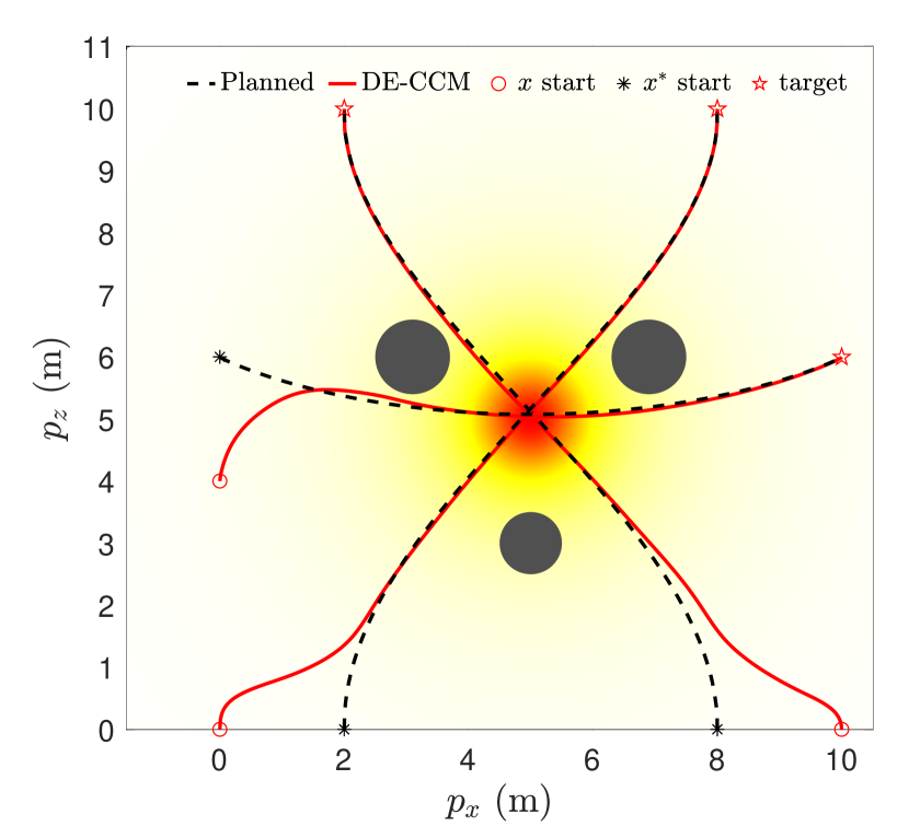
a No Learning

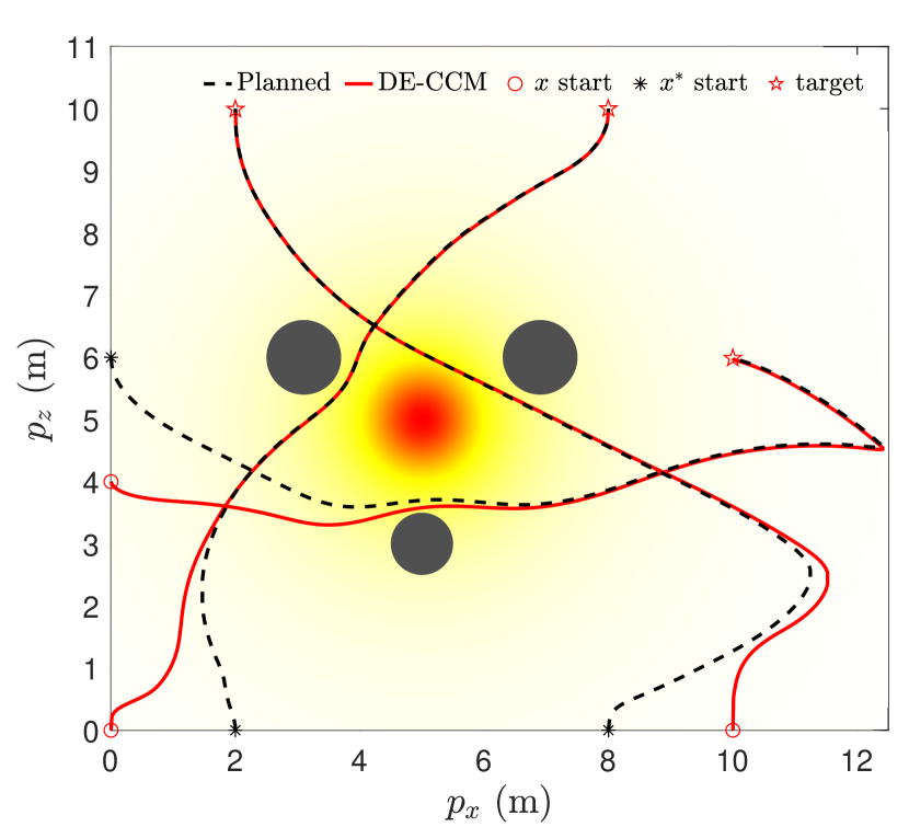
b Moderate Learning

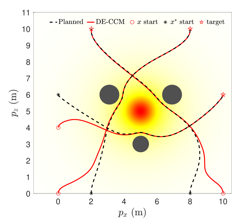
c Good Learning

Figure 1: Planned and executed trajectories of DE-CCM for Tasks 1$\sim$3 in the presence of no, moderate and good learning. Start points of planned and actual trajectories are intentionally set to be different.

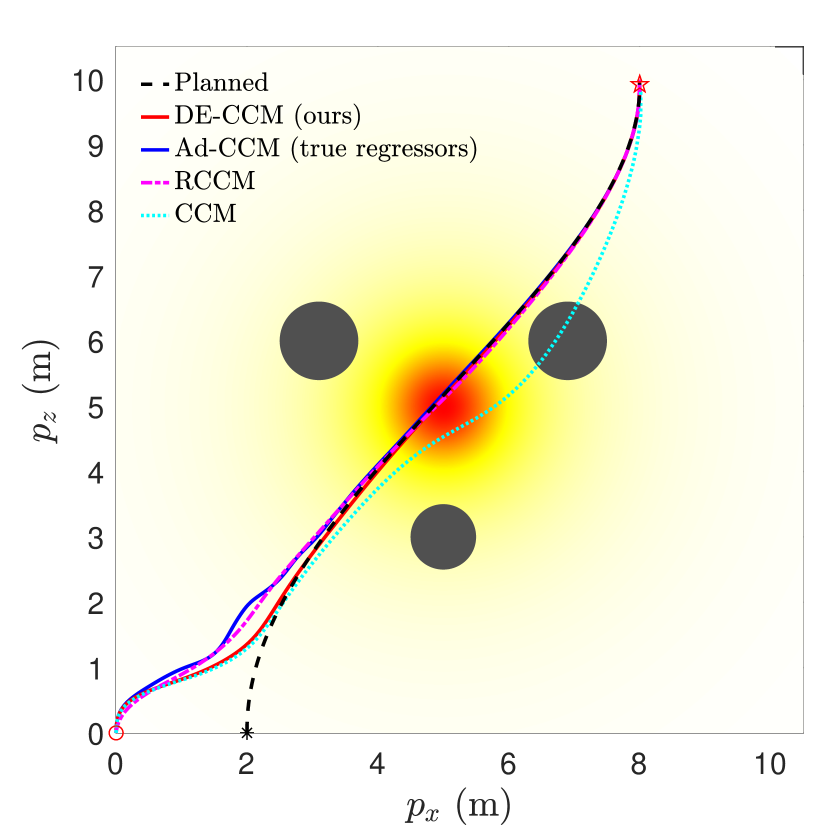
a No Learning

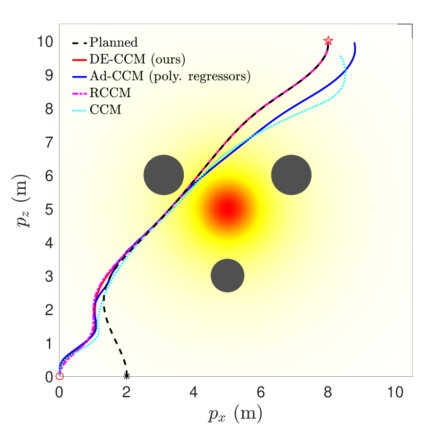
b Moderate Learning

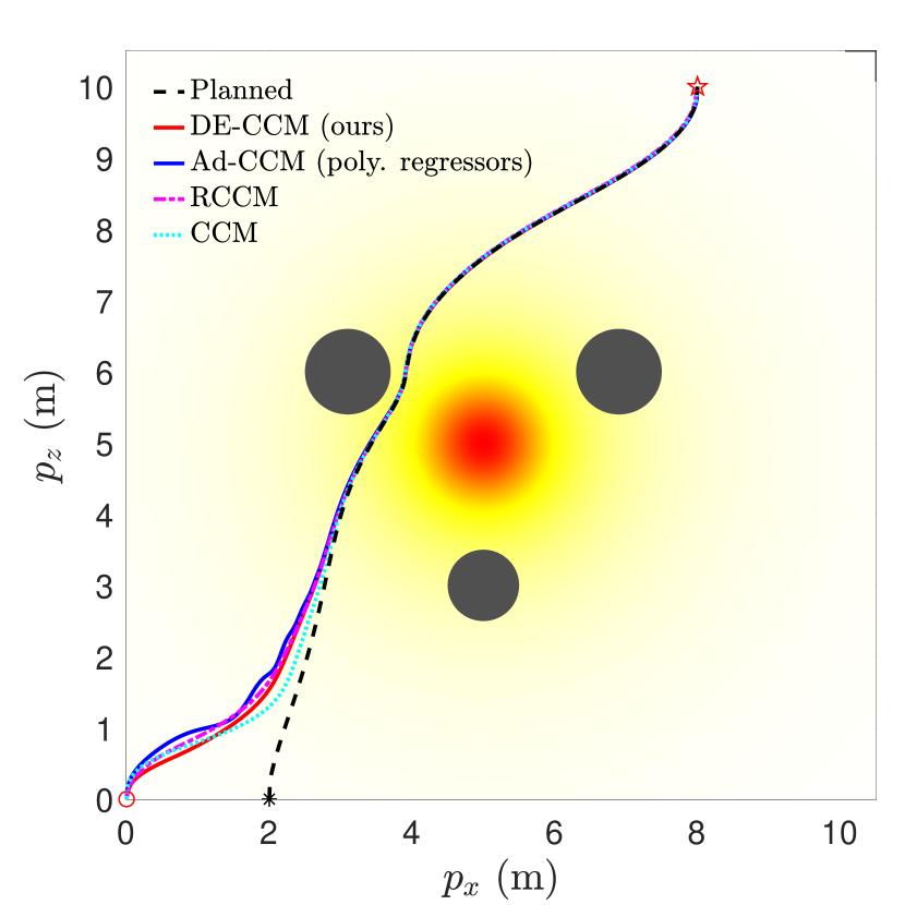
c Good Learning

Figure 2: Tracking performance of DE-CCM, Ad-CCM RCCM and CCM for Task 1 under different learning scenarios.

For the first experiments, we did not employ a low-pass filter to filter the estimated disturbance, which is equivalent to setting ${\mathcal{C}}(s)=I$ in 22. Figure 1 shows the planned and actual trajectories under the proposed controller based on the RRE condition and disturbance estimation, which we term as DE-CCM, in the presence of no, moderate and good learned model for uncertain dynamics. SN-DNNs (see Section III-A) with four inputs, two outputs and four hidden layers were used for all the learned models. For training data collection, we planned and executed nine trajectories with different start and end points as shown in Fig. 3. The tracking performance of the DE-CCM controller allow the quadrotor to safely explore the state space as long as the planned trajectories using the learned model are safe, as demonstrated in Fig. 3. The collected data during execution of these nine trajectories were used to train the moderate model. However, these nine trajectories were still not enough to fully explore the state space. For instance, the velocities of the quadrotor were not carefully controlled to cover the velocity range when planning the trajectories. Sufficient exploration of the state space is necessary to learn a good model for the uncertainty $d(x)$. As mentioned before, thanks to the performance guarantee (in terms of exponential trajectory convergence), the proposed DE-CCM controller can be used to control the system to safely explore the state space. For illustration purpose, we directly used true uncertainty model to generate the data and used the generated data for training, which yielded the good model.

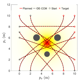
Figure 3: Safe exploration under the DE-CCM controller

One can see that the actual trajectories yielded by the DE-CCM controller converged to the desired trajectory as expected and almost overlapped with it afterward, throughout the learning phase, for all the three tasks. In fact, the slight deviations of actual trajectories from the desired ones under the DE-CCM controller were due to the finite step size associated with the ODE solver used for the simulations (see Remark 12). The planned trajectory for Task 2 in the moderate learning case seemed weird near the end point. This is because the learned model was not accurate in the area due to lack of sufficient exploration. However, with the DE-CCM controller, the quadrotor was still able to track the trajectory. Figure 4 depicts the trajectories of true, learned and estimated disturbances in the presence of no and good learning for Task 1, while the trajectories for Tasks 2 and 3 are similar and thus omitted. One can see that the estimated disturbances were always fairly close to the true disturbances. Also, the area with high disturbance intensity was avoided during path planning with good learning, which explains the smaller disturbance encountered.

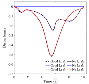
Figure 4: Trajectories of true, learned and estimated disturbances in the presence of no and good learning for Task 1. The notations $d_{1}$, $\hat{d}_{1}$ and $\check{d}_{1}$ denote the first element of $d$, $\hat{d}$ and $\check{d}$, respectively.

For comparison, we also implemented three other controllers, namely, a standard CCM controller, that ignores the uncertainty or learned model error, an adaptive CCM (Ad-CCM) controller from [3] that compensates for the learned model error, and finally a robust CCM (RCCM) controller that can be seen as a specific case of an DE-CCM controller with the disturbance estimate equal to zero and the EEB equal to the disturbance bound $b_{d}$. Since the Ad-CCM controller [3] needs a parametric structure for the uncertainty in the form of $\Phi(x)\theta$ with $\Phi(x)$ being a known regressor matrix and $\theta$ being the vector of unknown parameters. For the no learning case, we assume that we know the regressor matrix for the original uncertainty $d(x)$ and set it according to 51. For the learning cases, since we do not know the regressor matrix for the learned model error $\tilde{d}(x)$, we use a 2nd-order polynomial regressor matrix defined in 52.

$$\Phi(x)= \frac{1}{1+(x-5)^{2}+(z-5)^{2}}\begin{bmatrix}v_{x}^{2}&v_{z}^{2}\\ v_{x}^{2}&v_{z}^{2}\end{bmatrix}$$ (51)

$$\Phi(x)= \begin{bmatrix}1\\ 1\end{bmatrix}\begin{bmatrix}1&x&x^{2}&z&z^{2}&v_{x}&v_{x}^{2}&v_{z}&v_{z}^{2}\end{bmatrix}.$$ (52)

Figure 2 shows the tracking control performances yielded by these additional controllers for Task 1 under different learning scenarios. One can see that the actual trajectories yielded by the CCM controller deviated quite a lot from the planned ones and collided with obstacle sometimes, except in the case of good learning. Ad-CCM yields poor tracking performance under the moderate learning case. This is because the uncertainty $\tilde{(}x)$ may not have a parametric structure, or even if it does, the regressor matrix in 52 may not be sufficient to represent it. RCCM achieves a similar performance as compared to the proposed method, but shows a weaker robustness against control input delays, as demonstrated later.

We further evaluated the costs $J$ associated with the actual trajectories given by the DE-CCM controller under different learning qualities. The results are shown in Fig. 5. As expected, the good model helped plan better trajectories, which led to reduced costs for all the three tasks. It is not a surprise that the poor and moderate models led to temporal increase of the costs for some tasks. In practice, we may never use the poorly learned model, due to lack of a sufficient exploration of the state space, directly for planning trajectories. The proposed control approach ensures that in case one really does so, the planned trajectories can still be well tracked.

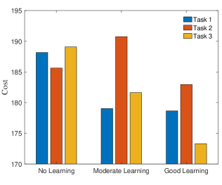
Figure 5: Costs of the actual trajectories yielded by the DE-CCM controller throughout the learning phase

We next tested the robustness of RCCM and DE-CCM against input delays under different learning scenarios. Note that unlike linear systems for which gain and phase margins are commonly used as robustness criteria, we often evaluate the robustness of nonlinear systems in terms of their tolerance for input delays. Under an input delay of $\Delta t$, the plant dynamics 1 becomes $\dot{x}=f(x)+B(x)\left(u(t-\Delta t)+d(x\right)$. For the following experiments, we leveraged a low-pass filter ${\mathcal{C}}(s)=\frac{30}{s+30}I_{2}$ to filter the estimated disturbance following 22. However, we kept using the same EEB of 0.1 as in the previous experiment. The Riemann energy, which indicates the tracking performance for all states, under these scenarios, is shown in Fig. 6. One can see that under input delays of both 10 ms and 30 ms, DE-CCM achieves smaller and less-oscillatory Riemann energy, indicating better robustness and tracking performance, compared to RCCM.

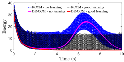
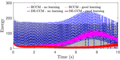
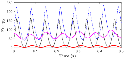
Figure 6: Riemann Energy yielded by DE-CCM and RCCM under input delays of 10 ms (top), and 30 ms (middle) with a zoomed-in plot (bottom). Learning improves the robustness of both DE-CCM and RCCM against input delays.

Additionally, the robustness of DE-CCM against input delays in the presence of good learning is significantly improved compared to the no-learning case, which illustrates the benefits of incorporating learning. This can be explained as follows. Notice that the input delay may cause the disturbance estimate $\check{d}^{0}(t)$ to be highly oscillatory and a large discrepancy between $\check{d}^{0}(t)$ and $d(x(t))$. The low pass filter ${\mathcal{C}}(s)$ can filter out high-frequency oscillatory component of $\check{d}^{0}(t)$. Under good learning, according to 22, the learned model $\hat{d}(x(t))$ approaches the true uncertainty $d(x(t))$. As a result, under good learning, the filtered disturbance estimate $\check{d}(t)$ defined in 27 can be much closer to $d(x(t))$ leading to improved robustness and performance, compared to other learning cases.

VI Conclusions

This paper presents a trajectory-centric learning control framework based on contraction metrics and disturbance estimation for uncertain nonlinear systems. The framework allows for the use of deep neural networks (DNNs) (and many other model learning tools), to learn uncertain dynamics, while still providing guarantees of transient tracking performance in the form of exponential convergence of actual trajectories to desired ones throughout the learning phase, including the special case of no learning. On the other hand, with improved accuracy, the learned model can help improve the robustness of the tracking controller, e.g., against input delays, and plan better trajectories with improved performance beyond tracking. The proposed framework is demonstrated on a planar quadrotor example.

In the future, we would like to consider more general uncertainties, in particular, unmatched uncertainties that widely exist in practical systems. Additionally, in practice, a poorly learned model, if naively incorporated in a trajectory planner, may produce a trajectory that deviates much from the trajectories with which the collected data is associated, and necessitates large control inputs exceeding the actuator limits to track. To mitigate this issue, we will incorporate mechanisms to ensure that newly planned trajectories are close to data-collection trajectories. Finally, we would like to experimentally validate the proposed framework on real hardware.

-A Proof of Lemma 4

Hereafter, we use the notations $\mathbb{Z}_{i}$ and $\mathbb{Z}_{1}^{n}$ to denote the integer sets $\{i,i+1,i+2,\cdots\}$ and $\{1,2,\cdots,n\}$, respectively. Additionally, for notation brevity, we define $\sigma(t)\triangleq B(x(t))d(x(t))$. From (1) and (14), the prediction error dynamics are obtained as

$$\dot{\tilde{x}}(t)=-a\tilde{x}(t)+\hat{\sigma}(t)-\sigma(t),\quad\tilde{x}(0)=0.$$ (53)

Note that $\hat{\sigma}(t)=0$ (and thus $\check{d}^{0}(t)=0$ due to 16) for any $t\in[0,T)$ according to (15). Further considering the bound on $d(x)$ in (1), we have

$$\mathinner{\!\left\lVert\check{d}^{0}(t)-\hat{d}(x(t))\right\rVert}\leq b_{d},\quad\forall t\in[0,T).$$ (54)

We next derive the bound on $\mathinner{\!\left\lVert\hat{\sigma}(t)-\sigma(t)\right\rVert}$ for $T\leq t\leq\xi$. For any $t\in[iT,(i+1)T)$ ($i\in\mathbb{Z}_{0}$), we have

$$\tilde{x}(t)=e^{-a(t-iT)}\tilde{x}(iT)+\int_{iT}^{t}e^{-a(t-\tau)}(\hat{\sigma}(\tau)-\sigma(\tau))d\tau.$$

Since $\tilde{x}(t)$ is continuous, the preceding equation implies

$$\tilde{x}((i+1)T)=~{}e^{-aT}\tilde{x}(iT)+\!\int_{iT}^{(i+1)T}\!e^{-a((i+1)T-\tau)}d\tau\hat{\sigma}(iT)$$

$$-\!\int_{iT}^{(i+1)T}\!e^{-a((i+1)T-\tau)}\sigma(\tau)d\tau$$

$$\!=\!~{}e^{-aT}\tilde{x}(iT)\!+\!\frac{1\!-\!e^{-aT}}{a}\hat{\sigma}(iT)\!-\!\!\int_{iT}^{(i+1)T}\!\!\!e^{-a((i+1)T-\tau)}\sigma(\tau)d\tau$$

$$=~{}-\int_{iT}^{(i+1)T}e^{-a((i+1)T-\tau)}\sigma(\tau)d\tau,$$ (55)

where the first and last equalities are due to the estimation law (15).

Since $x(t)$ is continuous, $\sigma(t)~{}(=B(x)d(x))$ is also continuous given Assumption 1. Furthermore, considering that $e^{-a((i+1)T-\tau)}$ is always positive, we can apply the first mean value theorem in an element-wise manner to (55), which leads to

$$\tilde{x}((i+1)T)= -\int_{iT}^{(i+1)T}e^{-a((i+1)T-\tau)}d\tau\bm{[}\sigma_{j}(\tau_{j}^{*})\bm{]}$$

$$= -\frac{1}{a}(1-e^{-aT})\bm{[}\sigma_{j}(\tau_{j}^{*})\bm{]},$$ (56)

for some $\tau_{j}^{*}\in(iT,(i+1)T)$ with $j\in\mathbb{Z}_{1}^{n}$ and $i\in\mathbb{Z}_{0}$, where $\sigma_{j}(t)$ is the $j$-th element of $\sigma(t)$, and

$$\bm{[}\sigma_{j}(\tau_{j}^{*})\bm{]}\triangleq[\sigma_{1}(\tau_{1}^{*}),\cdots,\sigma_{n}(\tau_{n}^{*})]^{\top}.$$

The estimation law (15) indicates that for any $t$ in $[(i+1)T,(i+2)T)\cap[0,\xi]$, we have $\hat{\sigma}(t)=-\frac{a}{e^{aT}-1}\tilde{x}((i+1)T).$ The preceding equality and (56) imply that for any $t$ in $[(i+1)T,(i+2)T)\cap[0,\xi]$ with $i\in\mathbb{Z}_{0}$, there exist $\tau_{j}^{*}\in(iT,(i+1)T)$ ($j\in\mathbb{Z}_{1}^{n}$) such that

$$\hat{\sigma}(t)=e^{-aT}\bm{[}\sigma_{j}(\tau_{j}^{*})\bm{]}.$$ (57)

Note that

$$\mathinner{\!\left\lVert\sigma(t)\!-\!\bm{[}\sigma_{j}(\tau_{j}^{*})\bm{]}\right\rVert}\!\leq\!\sqrt{n}\left\lVert\sigma(t)\!-\!\bm{[}\sigma_{j}(\tau_{j}^{*})\bm{]}\right\rVert_{\infty}\!$$

$$= ~{}\!\sqrt{n}\mathinner{\!\left\lvert\sigma_{\bar{j}_{t}}(t)-{\sigma_{\bar{j}_{t}}(\tau_{\bar{j}_{t}}^{*})}\right\rvert}\leq\!\sqrt{n}\mathinner{\!\left\lVert\sigma(t)-{\sigma(\tau_{\bar{j}_{t}}^{*})}\right\rVert},$$ (58)

where $\bar{j}_{t}=\arg\max_{j\in\mathbb{Z}_{1}^{n}}\mathinner{\!\left\lvert\sigma_{j}(t)-{\sigma_{j}(\tau_{j}^{*})}\right\rvert}$. Similarly,

$$\mathinner{\!\left\lVert\bm{[}\sigma_{j}(\tau_{j}^{*})\bm{]}\right\rVert}\leq \sqrt{n}\left\lVert\bm{[}\sigma_{j}(\tau_{j}^{*})\bm{]}\right\rVert_{\infty}=\sqrt{n}\mathinner{\!\left\lvert{\sigma_{{\hat{j}}}(\tau_{{\hat{j}}}^{*})}\right\rvert}$$

$$\leq \sqrt{n}\mathinner{\!\left\lVert{\sigma(\tau_{{\hat{j}}}^{*})}\right\rVert}\leq\sqrt{n}b_{d}\max_{x\in\mathcal{X}}\mathinner{\!\left\lVert B(x)\right\rVert},$$ (59)

where ${\hat{j}}=\arg\max_{j\in\mathbb{Z}_{1}^{n}}\mathinner{\!\left\lvert{\sigma_{j}(\tau_{j}^{*})}\right\rvert}$ and the last inequality is due to the fact $\mathinner{\!\left\lVert B(x)d(x)\right\rVert}\leq\mathinner{\!\left\lVert B(x)\right\rVert}\mathinner{\!\left\lVert d(x)\right\rVert}$, $\tau_{{\hat{j}}}^{*}\in[0,\tau]$, and Assumption 1. Therefore, for any $t\in[(i+1)T,(i+2)T)\cap[0,\xi]$ ($i\in\mathbb{Z}_{0}$), we have

$$\mathinner{\!\left\lVert\sigma(t)\!-\!\hat{\sigma}(t)\right\rVert}=\mathinner{\!\left\lVert\sigma(t)\!-\!e^{-aT}[\sigma_{j}(\tau_{j}^{*})]\right\rVert}$$

$$\leq \mathinner{\!\left\lVert\sigma(t)\!-\![\sigma_{j}(\tau_{j}^{*})]\right\rVert}\!+\!(1\!-\!e^{-aT})\mathinner{\!\left\lVert[\sigma_{j}(\tau_{j}^{*})]\right\rVert}$$

$$\leq \sqrt{n}\mathinner{\!\left\lVert\sigma(t)\!-\!{\sigma(\tau_{\bar{j}_{t}}^{*})}\right\rVert}+\!(1\!-\!e^{-aT})\sqrt{n}b_{d}\max_{x\in\mathcal{X}}\mathinner{\!\left\lVert B(x)\right\rVert},$$ (60)

for some $\tau_{\bar{j}_{t}}^{*}\in(iT,(i+1)T)$, where the equality is due to (57), and the last inequality is due to (58) and (59). The dynamics (1) and 17 indicate that

$$\mathinner{\!\left\lVert\dot{x}(t)\right\rVert}\leq\mathinner{\!\left\lVert f(x)+B(x)u\right\rVert}+\mathinner{\!\left\lVert B(x)\right\rVert}\mathinner{\!\left\lVert d(x)\right\rVert}\leq\phi,$$ (61)

for any $t\in[0,\xi)$, where $\phi$ is defined in 21. The inequality (61) implies that

$$\mathinner{\!\left\lVert x(t)-x(\tau_{\bar{j}_{t}}^{*})\right\rVert} \leq(t-\tau_{\bar{j}_{t}}^{*})\mathinner{\!\left\lVert\dot{x}(c)\right\rVert}\leq\phi(t-\tau_{\bar{j}_{t}}^{*})\leq 2\phi T,$$

where the first inequality is due to the mean value theorem [36, p.113,Theorem 5.19], $c\in({\bar{j}_{t}}^{*},t)$ is a constant, and the last inequality is due to the fact that $t\in[(i+1)T,(i+2)T)\cap[0,\xi]$ and $\tau_{\bar{j}_{t}}^{*}\in(iT,(i+1)T)$. The preceding inequality and (1) indicate that

$$\left\|{\sigma(x(t))-\sigma(x(\tau_{{{\bar{j}}_{t}}}^{*}))}\right\|=\left\|B(x(t))\left({d(x(t))-d(x(\tau_{{{\bar{j}}_{t}}}^{*}))}\right)\right.$$

$$+\left.\left({B(x(t))-B(x(\tau_{{{\bar{j}}_{t}}}^{*}))}\right)d(x(\tau_{{{\bar{j}}_{t}}}^{*}))\right\|$$

$$\leq\left\|{B(x(t))}\right\|\left\|{d(x(t))-d(x(\tau_{{{\bar{j}}_{t}}}^{*}))}\right\|$$

$$\quad+\left\|{B(x(t))-B(x(\tau_{{{\bar{j}}_{t}}}^{*}))}\right\|\left\|{d(x(\tau_{{{\bar{j}}_{t}}}^{*}))}\right\|$$

$$\leq{L_{d}}\left\|{x(t)-x(\tau_{{{\bar{j}}_{t}}}^{*})}\right\|{\max_{x\in\mathcal{X}}}\left\|{B(x)}\right\|$$

$$\quad+{L_{B}}\left\|{x(t)-x(\tau_{{{\bar{j}}_{t}}}^{*})}\right\|b_{d}$$

$$\leq 2\phi T({L_{d}}{\max_{x\in\mathcal{X}}}\left\|{B(x)}\right\|+{L_{B}}b_{d}).$$ (62)

Finally, plugging (62) into (60) leads to

$$\mathinner{\!\left\lVert\sigma(t)\!-\!\hat{\sigma}(t)\right\rVert} \leq 2\sqrt{n}\phi T({L_{d}}{\max_{x\in\mathcal{X}}}\left\|{B(x)}\right\|\!+\!{L_{B}}b_{d})$$

$$+\!(1\!-\!e^{-aT})\sqrt{n}b_{d}\max_{x\in\mathcal{X}}\mathinner{\!\left\lVert B(x)\right\rVert}=\alpha(T),$$ (63)

for any $t\in[T,\xi]$. From (54), (63) and the relation between $\hat{\sigma}(t)$ and $\check{d}^{0}(t)$ in 16, we arrive at (20). Due to Assumption 1 and the assumption that $\mathcal{X}$ and $\mathcal{U}$ are compact, the constants involved in the definition of $\alpha(T)$ below 20 are all finite. As a result, we have $\lim_{T\rightarrow 0}\alpha(T)=0$, which further indicates that $\lim_{T\rightarrow 0}\bar{\delta}_{\textup{de}}^{0}(t)=0,$ for any $t\geq T$. The proof is complete. $\blacksquare$

References

• [1] Winfried Lohmiller and Jean-Jacques E Slotine “On contraction analysis for non-linear systems” In Automatica 34.6 Elsevier, 1998, pp. 683–696
• [2] Ian R Manchester and Jean-Jacques E Slotine “Control contraction metrics: Convex and intrinsic criteria for nonlinear feedback design” In IEEE TAC 62.6, 2017, pp. 3046–3053
• [3] Brett T Lopez and Jean-Jacques E Slotine “Adaptive nonlinear control with contraction metrics” In IEEE Control Systems Letters 5.1 IEEE, 2020, pp. 205–210
• [4] Arun Lakshmanan, Aditya Gahlawat and Naira Hovakimyan “Safe feedback motion planning: A contraction theory and $\mathcal{L}_{1}$-adaptive control based approach” In Proceedings of 59th IEEE CDC, 2020, pp. 1578–1583
• [5] Pan Zhao, Ziyao Guo and Naira Hovakimyan “Robust Nonlinear Tracking Control with Exponential Convergence Using Contraction Metrics and Disturbance Estimation” In Sensors 22.13, 2022, pp. 4743
• [6] Sumeet Singh et al. “Robust feedback motion planning via contraction theory” In The International Journal of Robotics Research, under review, 2019
• [7] Pan Zhao et al. “Tube-certified trajectory tracking for nonlinear systems with robust control contraction metrics” In IEEE Robotics and Automation Letters 7.2, 2022, pp. 5528–5535
• [8] Ian R Manchester and Jean-Jacques E Slotine “Robust control contraction metrics: A convex approach to nonlinear state-feedback $H_{\infty}$ control” In IEEE Control Systems Letters 2.3, 2018, pp. 333–338
• [9] Hiroyasu Tsukamoto, Soon-Jo Chung and Jean-Jaques E Slotine “Contraction theory for nonlinear stability analysis and learning-based control: A tutorial overview” In Annual Reviews in Control 52 Elsevier, 2021, pp. 135–169
• [10] Felix Berkenkamp and Angela P. Schoellig “Safe and robust learning control with Gaussian processes” In Proceedings of 2015 ECC, 2015, pp. 2496–2501
• [11] Guanya Shi et al. “Neural lander: Stable drone landing control using learned dynamics” In ICRA, 2019, pp. 9784–9790
• [12] Girish Chowdhary et al. “Bayesian nonparametric adaptive control using Gaussian processes” In IEEE Transactions on Neural Networks and Learning Systems 26.3, 2014, pp. 537–550
• [13] Aditya Gahlawat et al. $\mathcal{L}_{1}$-$\mathcal{GP}$: $\mathcal{L}_{1}$ Adaptive Control with Bayesian Learning” In L4DC, PLMR 120, 2020, pp. 1–12
• [14] Aditya Gahlawat et al. “Contraction $\mathcal{L}_{1}$ Adaptive Control using Gaussian Processes” In L4DC, PMLR 144, 2021, pp. 1027–1040
• [15] Lukas Hewing, Juraj Kabzan and Melanie N. Zeilinger “Cautious model predictive control using Gaussian process regression” In IEEE Transactions on Control Systems Technology, 2019
• [16] Anil Aswani et al. “Provably safe and robust learning-based model predictive control” In Automatica 49.5 Elsevier, 2013, pp. 1216–1226
• [17] Mohammad Javad Khojasteh et al. “Probabilistic safety constraints for learned high relative degree system dynamics” In L4DC, 2020, pp. 781–792
• [18] Glen Chou, Necmiye Ozay and Dmitry Berenson “Model error propagation via learned contraction metrics for safe feedback motion planning of unknown systems” In arXiv preprint arXiv:2104.08695, 2021
• [19] Girish Joshi and Girish Chowdhary “Deep model reference adaptive control” In Proc. CDC), 2019, pp. 4601–4608
• [20] Girish Joshi, Jasvir Virdi and Girish Chowdhary “Asynchronous deep model reference adaptive control” In Conference on Robot Learning, 2020, pp. 984–1000
• [21] Runhan Sun et al. “Lyapunov-based real-time and iterative adjustment of deep neural networks” In IEEE Control Systems Letters 6 IEEE, 2021, pp. 193–198
• [22] Omkar Sudhir Patil et al. “Lyapunov-derived control and adaptive update laws for inner and outer layer weights of a deep neural network” In IEEE Control Systems Letters 6 IEEE, 2021, pp. 1855–1860
• [23] Petros A. Ioannou and Jing Sun “Robust Adaptive Control” Mineola, NY: Dover Publications, Inc., 2012
• [24] Wen-Hua Chen et al. “Disturbance-observer-based control and related methods—-An overview” In IEEE Trans. Ind. Electron. 63.2, 2015, pp. 1083–1095
• [25] Takeru Miyato et al. “Spectral normalization for generative adversarial networks” In ICLR, 2018
• [26] Yujia Huang et al. “Training certifiably robust neural networks with efficient local lipschitz bounds” In NeurIPS 34, 2021, pp. 22745–22757
• [27] Karen Leung and Ian R. Manchester “Nonlinear stabilization via control contraction metrics: A pseudospectral approach for computing geodesics” In ACC, 2017, pp. 1284–1289
• [28] Manfredo Perdigao Do Carmo and J Flaherty Francis “Riemannian Geometry” Boston, MA, USA: Springer, 1992
• [29] Chengyu Cao and Naira Hovakimyan $\mathcal{L}_{1}$ adaptive output feedback controller for non strictly positive real reference systems with applications to aerospace examples” In AIAA Guidance, Navigation and Control Conference and Exhibit, 2008, pp. 7288
• [30] Pan Zhao et al. “Robust Adaptive Control of Linear Parameter-Varying Systems with Unmatched Uncertainties” In arXiv:2010.04600, 2021
• [31] Naira Hovakimyan and Chengyu Cao $\mathcal{L}_{1}$ Adaptive Control Theory: Guaranteed Robustness with Fast Adaptation” Philadelphia, PA: Society for IndustrialApplied Mathematics, 2010
• [32] Armin Lederer, Jonas Umlauft and Sandra Hirche “Uniform Error Bounds for Gaussian Process Regression with Application to Safe Control” In arXiv preprint arXiv:1906.01376, 2019
• [33] Randy Freeman and Petar V. Kokotovic “Robust Nonlinear Control Design: State-Space and Lyapunov Techniques” Springer Science & Business Media, 2008
• [34] Matthew Kelly “An introduction to trajectory optimization: How to do your own direct collocation” In SIAM Review 59.4 SIAM, 2017, pp. 849–904
• [35] Jonathan Currie and David I. Wilson “OPTI: Lowering the barrier between open source optimizers and the industrial MATLAB user” In Foundations of Computer-Aided Process Operations, 2012
• [36] Walter Rudin “Principles of Mathematical Analysis (3rd ed.)” New York: McGraw-Hill, 1976