UWThPh-2021-22

UTHEP-768

Yuhma Asano^† and Harold C. Steinacker^‡

^†Faculty of Pure and Applied Sciences, University of Tsukuba,
1-1-1 Tennodai, Tsukuba, Ibaraki 305-8571, Japan
Email: asano@het.ph.tsukuba.ac.jp
^‡Faculty of Physics, University of Vienna
Boltzmanngasse 5, A-1090 Vienna, Austria
Email: harold.steinacker@univie.ac.at

Abstract

We present a systematic study of spherically symmetric vacuum solutions of the IKKT matrix model, within the framework of semi-classical covariant quantum geometries. All asymptotically flat solutions of the equations of motion of the frame are found explicitly. They reproduce the linearized Schwarzschild geometry for large $r$ but deviate from it at the non-linear level, and include contributions from dilaton and axion. They are pertinent to the pre-gravity theory arising on classical brane solutions within the classical matrix model, before taking into account the Einstein-Hilbert term induced by quantum effects. We also address the problem of reconstructing matrix configurations corresponding to some given frame, and show that this problem can always be solved at the geometrical level of the underlying higher spin theory, ignoring possible higher spin modes.

1 Introduction

Matrix models have been introduced some 25 years ago as candidates for a non-perturbative formulation of superstring theory [1, 2]. They provide an independent and non-perturbative starting point, which allows to access the rich structures of string theory from a different angle. In particular, they yield solutions and configurations which are not easily seen from the more traditional point of view. Our approach is to take the IKKT or IIB matrix model as a starting point, and investigate the physics emerging on interesting background solutions.

A particularly interesting type of 3+1-dimensional covariant quantum space-time solution of the IKKT model was recently found [4, 5, 6], which is manifestly invariant under local rotations and translations. This type of solution is dynamical, and leads to a well-defined higher-spin gauge theory for the fluctuations on the background. The geometry is governed by a dynamical frame, which is generated by the dynamical matrices of the model in the semi-classical regime. A covariant description of the geometrical sector of this theory was obtained in [7] in terms of a Weitzenböck connection and its torsion. This was cast into a more conventional equation in terms of the dynamical frame and the Levi-Civita connection in [8]. This allows to look for solutions of these non-linear equations describing non-trivial geometries. A simple spherically symmetric static solution centered at some point was found, which is asymptotically flat and reduces to the linearized Schwarzschild solution for large $r$.

In the present paper, we present a systematic study of spherically symmetric vacuum solutions of the non-linear equations of motion for the frame. This is a rather non-trivial problem due to the presence of dilaton and (gravitational) axion, which lead to a coupled system of non-linear equations. Its solution is not unique, in contrast to general relativity (GR), where the Schwarzschild solution is unique by Birkhoff’s theorem. Despite the complicated structure, we obtain explicitly the most general vacuum solution, including non-trivial contributions from dilaton and (gravitational) axion. The generic solution is given in terms of a hypergeometric function ${}_{2}F_{1}$ involving a number of free parameters. The solutions with asymptotically flat geometry involve three independent parameters, which can be identified as mass, and two scales characterizing the axion and dilaton. They have an intricate global structure with various types of behavior depending on the parameters.

Even though all asymptotically flat solutions reduce to the linearized Schwarzschild geometry for large radius, none of the solutions appear to reproduce the characteristic features of a Schwarzschild-like horizon. The deviation from the Schwarzschild geometry is already seen in the Eddington-Robertson-Schiff parameters, which are found to be $\gamma=1$ but $\beta=2$ in all asymptotically flat solutions. This should not be too surprising, since we consider the semi-classical regime of the matrix model without taking into account quantum effects. Interestingly, we find some solutions which are reminiscent of wormhole geometries, connecting two asymptotically flat geometries.

These non-standard characteristics of the solutions are interpreted as features of the classical pre-gravity theory described by the classical matrix model, which is expected to dominate the extreme IR (cosmological) regime. In the presence of fuzzy extra dimensions, an Einstein-Hilbert (E-H) term arises in the quantum effective action as shown in [9], which is expected to dominate on shorter scales. Therefore the present solutions should be interpreted with caution. They certainly provide a deeper understanding of the classical aspects of the matrix model and its deviations from GR; however a proper physical assessment of the solutions can presumably only be given once this induced Einstein-Hilbert term is taken into account.

The solutions given in this paper are solutions of the equations of motion for the frame, and we also elaborate the corresponding metric in standard form. To obtain solutions of the (semi-classical) matrix model, it remains to be shown that these frames can be implemented in terms of Hamiltonian vector fields generated by the basic matrices. We also address this “reconstruction” problem and show that this can always be achieved at the lowest “geometrical” level of the underlying higher spin gauge theory, based on general results in [4, 10]. The extension to the full higher spin sector remains as an open problem, but we expect that this can be solved, as illustrated in the simplest solution found in [8].

This paper is organized as follows. After a brief review of the underlying matrix model and its geometrical interpretation in section 2, we discuss the general setup of spherically symmetric geometries in the present framework, and obtain the most general spherically symmetric solutions for the frame in section 4. The effective metric resulting from these solutions is then discussed in section 5. In appendix A, we provide a solution of the reconstruction problem at the geometrical level of the full higher spin theory. Finally, appendix B provides a compact derivation of the covariant equations of motion for the frame and its torsion.

2 Matrix model and cosmological quantum spacetime

We consider the IKKT or IIB matrix model [1] with a mass term,

$$S[Z,\Psi]={\rm Tr}\big{(}[Z^{\dot{\alpha}},Z^{\dot{\beta}}][Z_{{\dot{\alpha}}},Z_{{\dot{\beta}}}]+2m^{2}Z_{\dot{\alpha}}Z^{\dot{\alpha}}\,\,+\overline{\Psi}\Gamma_{\dot{\alpha}}[Z^{\dot{\alpha}},\Psi]\big{)}\ ,$$ (2.1)

where the indices are contracted with the flat metric $\eta_{\dot{\alpha}\dot{\beta}}$. Besides invariance under gauge transformations $Z^{\dot{\alpha}}\to U^{-1}Z^{\dot{\alpha}}U$, the model is invariant under $SO(9,1)$ acting on the dotted indices, and ${\cal N}=2$ supersymmetry when $m^{2}=0$. We will study classical solutions of this matrix model, which can be interpreted as spherically symmetric space-time geometries around some center, which for large distances reduce to the cosmological space-time solution found in [4]. That solution is given by

$$Z^{\dot{\alpha}}=\frac{1}{R}{\cal M}^{\dot{\alpha}4}=:T^{\dot{\alpha}},\qquad R^{-2}=\frac{1}{3}m^{2}\$$ (2.2)

for ${\dot{\alpha}}=0,...,3$, and requires the presence of the mass term in (2.1). Here ${\cal M}^{{\dot{\alpha}}{\dot{\beta}}}$ are $\mathfrak{so}(4,2)$ generators in the doubleton representation ${\cal H}_{n}$ for $n\in{\mathbb{N}}$. All matrices with indices from $4$ to $9$ as well as the fermions will be set to zero; nevertheless, they play a crucial role in the quantum theory. The mass $m^{2}$ sets the cosmological curvature scale, so that it effectively vanishes from a local point of view. Ultimately, it is expected that this solution (or a very similar one) is stabilized by quantum effects without mass term. However we restrict ourselves to the classical model in this paper, and therefore include the explicit mass term.

2.1 Semi-classical structure of the background

We consider a class of solutions of the matrix model, which admit a semi-classical interpretation in terms of a 6-dimensional Poisson (more precisely: symplectic) manifold ${\cal M}^{6}$, which can be viewed as a twisted $S^{2}$ bundle over space-time ${\cal M}^{3,1}$:

$${\cal M}^{6}\stackrel{{\scriptstyle\rm loc}}{{\cong}}{\cal M}^{3,1}\times S^{2}\ .$$ (2.3)

“Twisted” bundle, means that the local space-like stabilizer group $SO(3)$ of any point on ${\cal M}^{3,1}$ acts on the internal $S^{2}$. Such a background in the matrix model will be denoted as “covariant quantum space”. A specific example of such a solution where ${\cal M}^{3,1}$ is a cosmological FLRW space-time was given in [6] and discussed in detail in [4]. The most important feature of such a background in the matrix model is that the local bundle structure leads to a higher-spin gauge theory, where the gauge symmetry of the matrix model translates into (higher-spin generalization of) volume-preserving diffeomorphism.

It was shown in [7] that the semi-classical equations of motion of the matrix model can be translated into a covariant description of a frame and its associated Weitzenböck connection. That description, in turn, was re-cast in [8] in terms of covariant equations of motion for the frame, in terms of the standard Levi-Civita connection.

To be specific, we will mostly focus on local perturbations of the cosmological solution in [4], keeping the asymptotics fixed. However, most of the considerations are more general, and some of the solutions will correspond to more general asymptotic backgrounds. In particular, we find hints for solutions with global structure reminiscent of wormholes, and some special cases are expected to give rise to other cosmological asymptotics. Those aspects should be studied in detail elsewhere.

Cosmological FLRW background.

Let us describe the mathematical structure of the solution in [4] in some detail. The only mathematical structures which exist in the matrix model are the matrices $Z^{\dot{\alpha}}$ and their commutators, which reduce to functions and Poisson brackets in the semi-classical limit $n\to\infty$. We must learn how to work with these efficiently and to cast the system into a recognizable form.

The above background provides natural generators $x^{\mu}\sim X^{\mu}$ and $t^{\mu}\sim T^{\mu}$ which can be interpreted as functions on ${\mathbb{C}}P^{1,2}$, with a Poisson or symplectic structure $\{.,.\}$ encoded in $\theta^{\mu\nu}=\{x^{\mu},x^{\nu}\}$. The doubleton representations ${\cal H}_{n}$ entail constraints, which in the semi-classical limit imply the following relations

$$x_{\mu}x^{\mu} =-R^{2}-x_{4}^{2}=-R^{2}\cosh^{2}(\eta)\,,\qquad R\sim\frac{\tilde{R}}{2}n$$ (2.4a)

$$t_{\mu}t^{\mu} =\tilde{R}^{-2}\,\cosh^{2}(\eta)\,,$$ (2.4b)

$$t_{\mu}x^{\mu} =0,$$ (2.4c)

$$t_{\mu}\theta^{\mu\alpha} =-\sinh(\eta)x^{\alpha},$$ (2.4d)

$$x_{\mu}\theta^{\mu\alpha} =-\tilde{R}^{2}R^{2}\sinh(\eta)t^{\alpha},$$ (2.4e)

$$\eta_{\mu\nu}\theta^{\mu\alpha}\theta^{\nu\beta} =R^{2}\tilde{R}^{2}\eta^{\alpha\beta}-R^{2}\tilde{R}^{4}t^{\alpha}t^{\beta}+\tilde{R}^{2}x^{\alpha}x^{\beta}\ ,$$ (2.4f)

where $\mu,\alpha=0,\ldots,3$, and a self-duality relation for $\theta^{\mu\nu}$ [4]. The $x^{\mu}$ will be interpreted as Cartesian coordinate functions $x^{\mu}:\,{\cal M}^{3,1}\hookrightarrow{\mathbb{R}}^{3,1}$, and $\eta$ is a global time coordinate via

$$R\sinh(\eta)=\pm\sqrt{-x_{\mu}x^{\mu}-R^{2}}\ ,$$ (2.5)

which will be related to the scale parameter of the universe. Similarly, the $t^{\mu}$ are extra generators which describe the internal $S^{2}$ fiber over every point on ${\cal M}\equiv{\cal M}^{3,1}$. Together, $x^{\mu}$ and $t^{\mu}$ generate the algebra ${\cal C}\cong{\cal C}^{\infty}({\mathbb{C}}P^{1,2})$. Along with a selfduality relation, these constraints allow to express the Poisson tensor $\theta^{\mu\nu}$ as follows

$$\theta^{\mu\nu} =\frac{\tilde{R}^{2}}{\cosh^{2}(\eta)}\Big{(}\sinh(\eta)(x^{\mu}t^{\nu}-x^{\nu}t^{\mu})+\epsilon^{\mu\nu\alpha\beta}x_{\alpha}t_{\beta}\Big{)}\ .$$ (2.6)

Now consider the Poisson brackets:

$$\{x^{\mu},x^{\nu}\} =\theta^{\mu\nu}=-\tilde{R}^{2}R^{2}\{t^{\mu},t^{\nu}\}\ ,$$ (2.7)

$$\{t^{\mu},x^{\nu}\} =\eta^{\mu\nu}\sinh(\eta)\,.$$ (2.8)

This implies that

$$\{t^{\mu},.\}\ =\sinh(\eta)\partial_{\mu},$$ (2.9)

where $\partial_{\mu}:=\frac{\partial}{\partial x^{\mu}}$ act as momentum generators on ${\cal M}^{3,1}$, leading to the useful relation

$$\partial_{\mu}\phi=\beta\{t_{\mu},\phi\},\qquad\beta=\frac{1}{\sinh(\eta)}\ ,$$ (2.10)

for an arbitrary function $\phi=\phi(x)$. In the late time regime, the internal sphere and the Poisson tensor are characterized by [7]

$$|t| \approx\tilde{R}^{-1}\cosh(\eta)\ ,$$

$$\theta^{0i} \stackrel{{\scriptstyle\xi}}{{\approx}}\tilde{R}^{2}R\,t^{i}\ \gg\ \theta^{ij}\stackrel{{\scriptstyle\xi}}{{\approx}}\frac{\tilde{R}^{2}R}{\sinh(\eta)}\epsilon^{ijk}t^{k}\ \stackrel{{\scriptstyle\eta\to\infty}}{{\sim}}const\$$ (2.11)

near the reference point $\xi=(x^{0},0,0,0)$.

2.2 Frame and geometry on ${\cal M}^{3,1}$

The matrix model provides 3+1 generators $Z_{\dot{\alpha}}$, which define a frame on ${\cal M}^{3,1}$ via Here we use general coordinates $y^{\mu}$ that contain $x^{\mu}$. This defines a metric

$$\gamma^{\mu\nu}=\eta_{\dot{\alpha}\dot{\beta}}\tensor{E}{{}_{\dot{\alpha}}^{\mu}}\tensor{E}{{}_{\dot{\beta}}^{\nu}}.$$ (2.12)

Note that coordinate indices such as $\mu$ are raised and lowered by $\gamma_{\mu\nu}$, and frame indices such as $\dot{\alpha}$ by $\eta_{\dot{\alpha}\dot{\beta}}$. The effective metric $G^{\mu\nu}$ is then given by a conformal rescaling such that [4]

$$\sqrt{|G|}\rho^{-2}=\rho_{M},$$ (2.13)

where $|G|$ is the absolute value of the determinant of $G_{\mu\nu}$ and $\rho_{M}$ is the symplectic volume form (reduced to ${\cal M}^{3,1}$), which in Cartesian coordinates is $\rho_{M}=|\theta^{\mu\nu}|^{-\frac{1}{2}}=1/\sinh(\eta)$. Explicitly,

$$G^{\mu\nu}=\rho^{-2}\gamma^{\mu\nu}.$$ (2.14)

By definition, one can always make $\rho$ positive without loss of generality. For the cosmic background solution (2.2), the frame takes the form

$$\tensor{\bar{E}}{{}_{\dot{\alpha}}^{\mu}}=\sinh(\eta)\delta_{\dot{\alpha}}^{\mu}\ ,$$ (2.15)

and the dilaton is given by

$$\bar{\rho}^{2}=\sinh^{3}(\eta)\ .$$ (2.16)

More generally, the frame resulting from the above construction always satisfies the divergence constraint

$$\partial_{\nu}\big{(}\rho_{M}\tensor{E}{{}_{\dot{\alpha}}^{\nu}}\big{)}=\partial_{\nu}\big{(}\sqrt{|G|}\rho^{-2}\tensor{E}{{}_{\dot{\alpha}}^{\nu}}\big{)}=0=\nabla^{(G)}_{\nu}(\rho^{-2}\tensor{E}{{}_{\dot{\alpha}}^{\nu}})\ .$$ (2.17)

This can be seen as a consequence of the Jacobi identity [11, 8], and it means that the $\rho^{-2}\tensor{E}{{}_{\dot{\alpha}}^{\mu}}$ are volume-preserving vector fields.

Torsion tensor.

As usual, we can associate to the frame $\tensor{E}{{}_{\dot{\alpha}}^{\mu}}$ the co-frame

$$\tensor{E}{{}_{\dot{\alpha}}{}_{\mu}}=\gamma_{\mu\nu}\tensor{E}{{}_{\dot{\alpha}}^{\nu}}\ ,$$ (2.18)

which can be viewed as a one-form

$$E_{\dot{\alpha}}:=\tensor{E}{{}_{\dot{\alpha}}{}_{\mu}}dx^{\mu}\ .$$ (2.19)

Since the frame satisfies a divergence constraint (2.17), there is no local Lorentz invariance acting on the frame index. This means that the frame has more physical content than in GR. In particular, one can define the associated tensor or two-form

$$T^{\dot{\alpha}}:=dE^{\dot{\alpha}}=\frac{1}{2}\tensor{T}{{}_{\mu}{}_{\nu}^{\dot{\alpha}}}dx^{\mu}dx^{\nu}\ .$$ (2.20)

This can be understood as torsion of the Weitzenböck connection associated to the frame. Its totally antisymmetric component defines a rank one tensor via the Hodge star

$$\tilde{T}_{\rho}=\frac{1}{2}\sqrt{|G|}^{-1}\rho^{2}G_{\rho\kappa}\varepsilon^{\nu\sigma\mu\kappa}\tensor{T}{{}_{\nu}{}_{\sigma}{}_{\mu}}\ =\frac{1}{2}\sqrt{|\gamma|}^{-1}\gamma_{\rho\kappa}\varepsilon^{\nu\sigma\mu\kappa}\tensor{T}{{}_{\nu}{}_{\sigma}{}_{\mu}}\ ,$$ (2.21)

where $\tensor{T}{{}_{\nu}{}_{\sigma}{}_{\mu}}=\tensor{T}{{}_{\nu}{}_{\sigma}^{\dot{\alpha}}}\tensor{E}{{}_{\dot{\alpha}}{}_{\mu}}$. We shall denote $\tilde{T}_{\mu}$ as an axion one-form, for reasons explained in [8]. Moreover, the contraction of the torsion tensor is related to the dilaton through the following identity

$$\frac{2}{\rho}\partial_{\sigma}\rho\ =\tensor{T}{{}_{\mu}{}_{\sigma}^{\mu}}\ .$$ (2.22)

Equations of motion.

It was shown in [8] that the semi-classical equations of motion of the matrix model lead to the following equation of motion for the frame

$$\nabla^{(G)}_{\nu}(G^{\nu\rho}\rho^{2}\tensor{T}{{}_{\rho\mu}^{\dot{\alpha}}})=\frac{1}{2}\rho^{2}\sqrt{|G|}^{-1}\varepsilon^{\nu\rho\kappa\sigma}G_{\mu\kappa}\tilde{T}_{\sigma}\,\tensor{T}{{}_{\nu}{}_{\rho}^{\dot{\alpha}}}+m^{2}\tensor{E}{{}^{\dot{\alpha}}_{\mu}}\ .$$ (2.23)

See appendix B for details. These are analogous to Maxwell equations for the 4 vector fields $\tensor{E}{{}^{\dot{\alpha}}_{\mu}}$. Moreover, one can show using the equations of motion that the axion vector field is the derivative of a scalar field $\tilde{\rho}$ identified as gravitational axion,

$$\tilde{T}_{\mu}=\rho^{-2}\partial_{\mu}\tilde{\rho}\ ,$$ (2.24)

which satisfies

$$\sqrt{|G|}\nabla^{(G)}_{\nu}(G^{\mu\nu}\rho^{-4}\partial_{\mu}\tilde{\rho})=\frac{1}{4}\varepsilon^{\nu\rho\mu\kappa}\tensor{T}{{}_{\nu}{}_{\rho}^{\dot{\alpha}}}\tensor{T}{{}_{\kappa}{}_{\mu}{}_{\dot{\alpha}}}\ .$$ (2.25)

This can be written in terms of differential forms as follows

$$d*(\rho^{-4}d\tilde{\rho})=T^{\dot{\alpha}}\wedge T_{\dot{\alpha}}\ ,$$ (2.26)

where $*$ is the Hodge star associated with the effective metric $G$. Finally, the dilaton satisfies the following equation of motion as part of (2.23)

$$-\nabla^{(G)}_{\nu}\big{(}G^{\mu\nu}\rho^{-1}\partial_{\mu}\rho)=2\rho^{-2}m^{2}+\frac{1}{4}\rho^{2}\tensor{T}{{}_{\mu\rho}{}_{\kappa}}\tensor{T}{{}_{\nu}{}_{\sigma}^{\kappa}}G^{\mu\nu}G^{\rho\sigma}+\frac{1}{2}\rho^{-4}G^{\mu\nu}\partial_{\mu}\tilde{\rho}\partial_{\nu}\tilde{\rho}\ .$$ (2.27)

3 General rotationally invariant frame

We are interested in spherically symmetric static geometries centered at some point in space, which can be viewed as a local perturbation of the cosmic background solution (2.2). We assume that the scale of this local structure is much smaller than the cosmic background curvature, so that the background frame (2.15) can be approximated in Cartesian coordinates by

$$\tensor{E}{{}^{\dot{\alpha}}_{\mu}}\sim\frac{1}{\sinh(\eta)}\,\delta^{\dot{\alpha}}_{\mu}$$ (3.1)

for some fixed $\eta$, neglecting the cosmic time evolution. The $SO(3)$ symmetry around the local center acts on the cosmic background frame by treating $\dot{\alpha}$ as a vector index. Spherical symmetry will be imposed by keeping this $SO(3)$ symmetry manifest also for the perturbed frame. This is achieved in Cartesian coordinates centered at $r=0$ via the ansatz

$$\tensor{E}{{}^{0}_{0}} =A(r),$$

$$\tensor{E}{{}^{i}_{0}} =E(r)\,x^{i},$$

$$\tensor{E}{{}^{0}_{i}} =D(r)\,x^{i},$$

$$\tensor{E}{{}^{i}_{j}} =F(r)\,x^{i}x^{j}+\delta^{i}_{\ j}B(r)+S(r)\epsilon_{ijm}x^{m}\ ,$$ (3.2)

where $A,B,D,E,F$ and $S$ are functions of $r^{2}=\sum x_{i}^{2}$ only. Such a solution with $S=0$ and $E=0$ was found in [8], given by

$$\frac{1}{A} =1+\frac{2M}{r},\qquad B_{0}=b_{0},\qquad E=0=S,\qquad A\rho^{2}=const\ .$$ (3.3)

In this paper, we shall find the most general spherically symmetric static solution. $D$ and $F$ can be eliminated using a simple change of coordinates $t\to t+f(r)$ and $x^{i}\to g(r)x^{i}$, which is understood from now on. In terms of differential forms $\tensor{E}{{}^{\dot{\alpha}}}=\tensor{E}{{}^{\dot{\alpha}}_{\mu}}dx^{\mu}$, the frame is then

$$\tensor{E}{{}^{0}} =Adt,\qquad\tensor{E}{{}^{i}}=Bdx^{i}+Ex^{i}dt+S\epsilon_{ijm}x^{m}dx^{j}\ ,$$ (3.4)

and the associated torsion two-form $T^{\dot{\alpha}}=dE^{\dot{\alpha}}$ is obtained as

$$T^{0} =dE^{0}=A^{\prime}drdt,$$

$$T^{i} =dE^{i}=B^{\prime}drdx^{i}+Edx^{i}dt+x^{i}E^{\prime}drdt+S\epsilon_{ijm}dx^{m}dx^{j}+S^{\prime}\epsilon_{ijm}x^{m}drdx^{j}\ ,$$ (3.5)

where the prime denotes the derivative of functions with respect to $r$. Then the effective metric takes the form

$$G_{\mu\nu}=\rho^{2}\begin{pmatrix}-(A^{2}-r^{2}E^{2})&rBE&0&0\\ rBE&B^{2}&0&0\\ 0&0&r^{2}(B^{2}+r^{2}S^{2})&0\\ 0&0&0&r^{2}(B^{2}+r^{2}S^{2})\sin^{2}\vartheta\\ \end{pmatrix}\ ,$$ (3.6)

in the standard polar coordinates $(t,r,\vartheta,\varphi)$ with

$$\sqrt{|\gamma|}=|AB|(B^{2}+r^{2}S^{2})r^{2}\sin\vartheta\ .$$ (3.7)

Throughout this paper, we assume that $A$ and $B$ are positive for $r\to\infty$, since we are interested in perturbation of (3.1).

3.1 The general divergence constraint

We can solve the dilaton constraint (2.22) in the form

$$-\frac{2}{\rho}\partial_{\mu}\rho=\tensor{T}{{}_{\mu}{}_{\nu}^{\nu}}\ ,$$

for the most general ansatz as follows. Due to the spherical symmetry it suffices to consider the time and radial components, which reduce to the following two relations

$$0 =\frac{E}{B}\Big{(}\Big{(}\ln\Big{|}\frac{A}{rE}\Big{|}\Big{)}^{\prime}-\frac{2B^{2}}{r\left(B^{2}+r^{2}S^{2}\right)}\Big{)}\ ,$$

$$0 =\left[\ln\big{|}A\rho^{2}\left(B^{2}+r^{2}S^{2}\right)\big{|}\right]^{\prime}+\frac{2rS^{2}}{B^{2}+r^{2}S^{2}}\ .$$ (3.8)

The first equation has two branches: one with $E=0$ and one with $E\neq 0$.

Branch $E=0$.

In this case, the divergence constraint (3.8) reduces to only one differential equation. This can be rewritten as

$$(\ln|A|)^{\prime}=\frac{2B^{2}}{r(B^{2}+r^{2}S^{2})}-\left[\ln\big{(}r^{2}\rho^{2}\left(B^{2}+r^{2}S^{2}\right)\big{)}\right]^{\prime}\ .$$ (3.9)

Branch $E\neq 0$.

In this case, the difference of the above relations (3.8) can be integrated as

$$E=\frac{c_{e}}{r^{3}\rho^{2}\left(B^{2}+r^{2}S^{2}\right)}\ ,$$ (3.10)

for some integration constant $c_{e}$. Inserting this into the first equation gives

$$\left(\ln\Big{|}\frac{A}{rE}\Big{|}\right)^{\prime}=\frac{2}{c_{e}}r^{2}\rho^{2}B^{2}E\ .$$ (3.11)

The two equations can be written in the equivalent form

$$B^{2} =\frac{c_{e}}{2r^{2}\rho^{2}}\frac{\left(\ln\left|\frac{A}{rE}\right|\right)^{\prime}}{E}\ ,$$

$$S^{2} =-\frac{c_{e}}{2r^{4}\rho^{2}}\frac{\left(\ln\left|\frac{A}{r^{3}E}\right|\right)^{\prime}}{E}\ .$$ (3.12)

Hence $B(r)$ and $S(r)$ are determined by the two arbitrary functions $A(r)$ and $E(r)$. These should be determined by the equations of motion.

3.2 The axion

The axion one-form $\tilde{T}=\tilde{T}_{\mu}dx^{\mu}$ (2.21) can be obtained from

$$\frac{1}{2}T_{\nu\rho\mu}dx^{\nu}\wedge dx^{\rho}\wedge dx^{\mu}=T^{\dot{\alpha}}\wedge E_{\dot{\alpha}}\ =\rho^{-2}*\tilde{T}\ .$$ (3.13)

By using (3.5), one can rewrite $T^{\dot{\alpha}}\wedge T_{\dot{\alpha}}$ explicitly as

$$T^{0}\wedge E_{0} =0\ ,$$

$$T^{i}\wedge E_{i} =(B^{\prime}drdx^{i}+Edx^{i}dt)\wedge S\epsilon_{ijm}x^{m}dx^{j}+S\epsilon_{ijm}dx^{m}dx^{j}(Bdx^{i}+Ex^{i}dt)+S^{\prime}B\epsilon_{ijm}x^{m}drdx^{j}dx^{i}$$

$$=2(rB^{\prime}S-rS^{\prime}B-3SB)d^{3}x-2ES\epsilon_{mij}x^{m}dx^{i}dx^{j}dt\ ,$$ (3.14)

noting that

$$x^{i}\epsilon_{ijm}rdr\wedge dx^{j}\wedge dx^{m}=2r^{2}d^{3}x\ .$$ (3.15)

Through the following relation

$$rB^{\prime}S-rS^{\prime}B-3SB=rBS\left(\ln\Big{|}\frac{B}{r^{3}S}\Big{|}\right)^{\prime}\ ,$$ (3.16)

the $t$ and $r$ components of (3.13) reduce to

$$\gamma^{t\nu}\tilde{T}_{\nu} =\frac{2rBS(\ln\left|\frac{B}{r^{3}S}\right|)^{\prime}}{|AB|(B^{2}+r^{2}S^{2})}\ ,$$

$$\gamma^{r\nu}\tilde{T}_{\nu} =\frac{4rES}{|AB|(B^{2}+r^{2}S^{2})}\ ,$$ (3.17)

while all other components in $(t,r,\vartheta,\varphi)$ coordinates vanish. Hence the axion vanishes if $S=0$. Explicitly, this gives

$$\tilde{T}_{t} =\rho^{-2}\partial_{t}\tilde{\rho}=-\frac{2rBS}{|AB|(B^{2}+r^{2}S^{2})}\left(-r^{2}E^{2}\left(\ln\Big{|}\frac{B}{rS}\Big{|}\right)^{\prime}+A^{2}\left(\ln\Big{|}\frac{B}{r^{3}S}\Big{|}\right)^{\prime}\right)\ ,$$

$$\tilde{T}_{r} =\rho^{-2}\partial_{r}\tilde{\rho}=-\frac{2r^{2}EB^{2}S}{|AB|(B^{2}+r^{2}S^{2})}\left(\ln\Big{|}\frac{rS}{B}\Big{|}\right)^{\prime}\ .$$ (3.18)

In particular, the axion $\tilde{\rho}$ is static if and only if

$$(A^{2}-r^{2}E^{2})\left(\ln\Big{|}\frac{B}{rS}\Big{|}\right)^{\prime}=2r^{-1}A^{2}\ ,$$ (3.19)

or

$$\left(\ln\Big{|}\frac{B}{rS}\Big{|}\right)^{\prime}=\frac{2}{r}\frac{1}{1-\frac{r^{2}E^{2}}{A^{2}}}\ .$$ (3.20)

Therefore for a static axion we obtain

$$\tilde{T}_{r} =\rho^{-2}\partial_{r}\tilde{\rho}=\frac{2r^{2}EB^{2}S}{|AB|(B^{2}+r^{2}S^{2})}\frac{2}{r}\frac{1}{1-\frac{r^{2}E^{2}}{A^{2}}}\ .$$ (3.21)

Taking into account the divergence constraint (3.10), this reduces to

$$\tilde{T}_{r} =\frac{4r^{4}\rho^{2}E^{2}B^{2}S}{c_{e}|AB|}\frac{1}{1-\frac{r^{2}E^{2}}{A^{2}}}\ .$$ (3.22)

The equation of motion for the axion.

It turns out that the equation of motion (2.25) for the axion holds identically for any spherically invariant configuration. This can be seen explicitly in Cartesian coordinates, where the right-hand side of (2.26) is obtained using (3.15) as

$$T^{\dot{\alpha}}\wedge T_{\dot{\alpha}} =T^{i}\wedge T^{j}\delta_{ij}=4\big{(}3ES+r(S^{\prime}E+SE^{\prime})\big{)}dtd^{3}x$$

$$=4SE\big{(}3+r\frac{d}{dr}\ln|SE|\big{)}d^{4}x=4rSE\big{(}\ln|r^{3}SE|\big{)}^{\prime}d^{4}x,$$ (3.23)

while the left-hand side of (2.26) is obtained using (2.24) and (3.17) as

$$d*(\rho^{-4}d\tilde{\rho}) =-\sqrt{|G|}\nabla^{(G)}_{\mu}(G^{\mu\nu}\rho^{-4}\partial_{\nu}\tilde{\rho})d^{4}x=-\partial_{\mu}\big{(}\rho^{-2}\sqrt{|G|}G^{\mu\nu}\tilde{T}_{\nu}\big{)}d^{4}x$$

$$=-\frac{1}{2}\partial_{\mu}\big{(}\varepsilon^{\nu\sigma\eta\mu}\tensor{T}{{}_{\nu}{}_{\sigma}{}_{\eta}}\big{)}d^{4}x=\partial_{i}(4SEx^{i})d^{4}x=4rSE\big{(}\ln|r^{3}SE|\big{)}^{\prime}d^{4}x\ .$$

Therefore the equation of motion (2.25) for the axion holds identically.

4 Solving the geometric equations of motion

4.1 The $E\neq 0$ solutions

In this section, we derive the general solutions for $E\neq 0$, using the divergence constraint (3.12). For the most general ansatz (3.2), the equation of motion (2.23) for $\dot{\alpha}=0$ and $\mu=r$ gives a second order differential equation, which can be reduced to

$$\left(\rho(\ln|A|)^{\prime}\right)^{2}=\frac{c_{0}^{2}c_{e}}{2}E\left(\ln\Big{|}\frac{A}{rE}\Big{|}\right)^{\prime}\ ,$$ (4.1)

for an arbitrary real constant $c_{0}$. Note that both sides of (4.1) are positive since $(\ln|\frac{A}{rE}|)^{\prime}$ is positive, as seen from (3.10) and (3.11), and $c_{e}E$ is positive by definition (3.10). Combining this with the divergence constraint (3.11), we obtain the relations

$$(\ln|A|)^{\prime} =c_{0}rBE\ ,$$

$$(\ln|rE|)^{\prime} =-\frac{2r^{2}B^{2}E\rho^{2}}{c_{e}}+c_{0}rBE\ .$$ (4.2)

Then the combination of the equation of motion for ${\dot{\alpha}}=0$ and $\mu=t$ with (4.1) implies $m=0$, which is assumed as an approximation in the present static setup. The equation of motion for ${\dot{\alpha}}=i$ and $\mu=t$ with the condition (3.20) for a static axion leads to

$$(\ln|rB|)^{\prime} =-\frac{1}{r}\frac{1}{r^{2}\frac{E^{2}}{A^{2}}-1}\ ,$$ (4.3)

using the above relations (4.1) and (4.2). Then the difference between (3.20) and (4.3) gives

$$(\ln|r^{2}S|)^{\prime}=\frac{1}{r}\frac{1}{r^{2}\frac{E^{2}}{A^{2}}-1}\ ,$$ (4.4)

which can be written only by $A$ and $E$ using (3.12). By eliminating the derivatives of $A,E$ and then $B$ in (4.4) using (4.2) and (4.3), one obtains

$$(\ln\rho)^{\prime} =-\frac{1}{2}\left(\frac{2}{r^{2}\frac{E^{2}}{A^{2}}-1}\Big{(}\frac{1}{r}-\frac{2r^{2}B^{2}E\rho^{2}}{c_{e}}\Big{)}-\frac{2r^{2}B^{2}E\rho^{2}}{c_{e}}+c_{0}rBE\right)$$

$$=-\frac{1}{r^{2}\frac{E^{2}}{A^{2}}-1}\Big{(}\frac{1}{r}-\frac{2r^{2}B^{2}E\rho^{2}}{c_{e}}\Big{)}-\frac{1}{2}(\ln|rE|)^{\prime}\ ,$$ (4.5)

and hence

$$(\ln|rE\rho^{2}|)^{\prime} =-\frac{2}{r^{2}\frac{E^{2}}{A^{2}}-1}\Big{(}\frac{1}{r}-\frac{2r^{2}B^{2}E\rho^{2}}{c_{e}}\Big{)}.$$ (4.6)

The equations of motion (2.23) for ${\dot{\alpha}}=i$ and $\mu=r$ and those for any $\dot{\alpha}$ and $\mu=\vartheta$, $\varphi$ are automatically satisfied if the above equations are satisfied.

We have therefore obtained a coupled system of 4 nonlinear differential equations for 4 functions $A(r),B(r),E(r)$ and $\rho(r)$. Solving such a system seems like a formidable task. Remarkably, the general solution can be obtained rather explicitly. To achieve this, we combine the above equations to get

$$\left(\ln\Big{|}\frac{E\rho^{2}}{rB^{2}}\Big{|}\right)^{\prime} =\frac{4}{r^{2}\frac{E^{2}}{A^{2}}-1}\frac{r^{2}B^{2}E\rho^{2}}{c_{e}}=-\left(\ln\left|\frac{A^{2}}{r^{2}E^{2}}-1\right|\right)^{\prime},$$ (4.7)

using (3.11) in the second step. This can be integrated as

$$\frac{E\rho^{2}}{rB^{2}}\left(\frac{A^{2}}{r^{2}E^{2}}-1\right) =c_{1}$$ (4.8)

for some constant $c_{1}$, so that

$$\boxed{\ \frac{A^{2}}{r^{2}E^{2}}=1+c_{1}\frac{rB^{2}}{E\rho^{2}}\ .}$$ (4.9)

Then, (4.9) and (4.3) gives

$$(\ln|B|)^{\prime} =\frac{E\rho^{2}}{c_{1}r^{2}B^{2}}\ .$$ (4.10)

Together with (4.7) we obtain

$$\frac{1}{E\rho^{2}}\left(\ln\Big{|}\frac{E\rho^{2}}{r}\Big{|}\right)^{\prime}+\frac{4}{c_{e}c_{1}}rE\rho^{2} =\frac{2}{c_{1}}\frac{1}{r^{2}B^{2}}-\frac{4}{c_{e}}r^{2}B^{2}\ .$$ (4.11)

Rewriting $E\rho^{2}$ by $B^{2}$ using (4.10) leads to a second-order ordinary differential equation (ODE) for $B$, which is solved by

$$\boxed{\ -|B|^{4c_{3}}\left((c_{3}+1)c_{e}\ \frac{1}{r^{4}}+c_{1}B^{4}\right)=c_{2}\ ,\ }$$ (4.12)

for arbitrary integration constants $c_{2}$ and $c_{3}$. Hence $B=B(r)$ satisfies a simple algebraic relation, which can in fact be solved explicitly for $r$ as a function of $B$:

$$r^{4}=\frac{-(c_{3}+1)c_{e}}{c_{1}B^{4}+c_{2}|B|^{-4c_{3}}}\ .$$ (4.13)

The other equation for the integration constants $c_{2}$ and $c_{3}$ can be obtained by differentiation of (4.12). The differentiation leads to

$$(\ln|B|)^{\prime} =\frac{1}{r}\frac{c_{e}}{c_{1}r^{4}B^{4}+c_{3}c_{e}},$$ (4.14)

for $B\neq 0$. Together with (4.10), one can derive an algebraic expression for $E\rho^{2}$ in terms of $B$ and $r$:

$$E\rho^{2}=c_{1}c_{e}\frac{rB^{2}}{c_{1}\,r^{4}B^{4}+c_{3}c_{e}}\ .$$ (4.15)

Then $\frac{A^{2}}{E^{2}}$ is obtained explicitly from (4.9) as

$$\frac{A^{2}}{r^{2}E^{2}}=\frac{1}{c_{e}}\big{(}(1+c_{3})c_{e}+c_{1}\,r^{4}B^{4}\big{)}\ .$$ (4.16)

Using (4.12), this can be written more compactly as

$$\boxed{\ r^{6}E^{2}=-\frac{c_{e}}{c_{2}}A^{2}|B|^{4c_{3}}\ .}$$ (4.17)

It remains to solve one more equation for $E$ (or $A$), but this can no longer be achieved in algebraic form. However, we can combine (4.3) and (4.2) for $B$ and $E$ with the above results to obtain

$$(\ln|r^{2}BE|)^{\prime} =-\frac{1}{r}\frac{1}{r^{2}\frac{E^{2}}{A^{2}}-1}-\frac{2r^{2}B^{2}E\rho^{2}}{c_{e}}+c_{0}rBE\ .$$ (4.18)

Together with (4.9) and (4.15), one obtains

$$(\ln|rBE|)^{\prime}-c_{0}rBE =-\frac{1}{r}\frac{2c_{1}r^{4}B^{4}-c_{e}}{c_{1}r^{4}B^{4}+c_{3}c_{e}}\ .$$ (4.19)

This still involves $B,E$ and $r$. However, combining this equation with (4.14) in the form

$$B\frac{d\ln|rB|}{dB} =1+c_{3}+\frac{c_{1}}{c_{e}}(rB)^{4},$$ (4.20)

one can rewrite it as

$$\frac{1}{(rE)^{2}}\frac{d(rE)}{d(rB)} =c_{0}-\frac{c_{0}c_{e}+2c_{1}(rB)^{3}\frac{1}{rE}}{c_{e}(1+c_{3})+c_{1}(rB)^{4}}\ ,$$ (4.21)

which is an ODE relating $(rB)$ and $(rE)$. We now introduce the effective radius

$$\tilde{r}^{2}:=\frac{c_{e}}{rE}=G_{\vartheta\vartheta}=\frac{G_{\varphi\varphi}}{\sin^{2}\vartheta}\$$ (4.22)

(cf. (5.6)), which is positive since $E/c_{e}>0$. Then the above equation takes the form of a non-linear ODE relating $\tilde{r}^{2}$ and $(rB)$:

$$\frac{d\tilde{r}^{2}}{d(rB)} =\frac{2c_{1}(rB)^{3}\,\tilde{r}^{2}+c_{0}c_{e}^{2}}{c_{e}(1+c_{3})+c_{1}(rB)^{4}}\ -c_{0}c_{e}\ .$$ (4.23)

This can be integrated in terms of the hypergeometric function ${}_{2}F_{1}(\frac{1}{4},\frac{1}{2};\frac{5}{4};z)$ as follows

$$\boxed{\ \tilde{r}^{2}=-\Big{(}\frac{(c_{3}+1)c_{e}}{c_{1}}\Big{)}^{\frac{1}{4}}\frac{c_{0}c_{e}z}{2(c_{3}+1)}\left((2c_{3}+1)\sqrt{1+z^{4}}\,_{2}F_{1}\Big{(}\frac{1}{4},\frac{1}{2};\frac{5}{4};-z^{4}\Big{)}-1\right)+c_{4}\sqrt{1+z^{4}}\ ,\ }$$ (4.24)

where $c_{4}$ is a new integration constant arising from the homogeneous term, and we define

$$rB=\Big{(}\frac{(c_{3}+1)c_{e}}{c_{1}}\Big{)}^{\frac{1}{4}}\,z\ ,$$ (4.25)

for better readability. One can then verify that all components of the equation of motion are satisfied including the equations (2.27) and (2.25) for the dilaton and the axion, respectively. We have therefore obtained the general solution for the case of $E\neq 0$.

Let us briefly take a look at some constraints on the functions and the parameters. The physical regime, which we will focus on in the following, is

$$c_{3}\geq 0\ ,\qquad c_{e}c_{1}>0\ ,\qquad c_{e}c_{2}<0\ .$$ (4.26)

These arise as follows: As noted before, $c_{e}$ has the same sign as $E$ by definition, (3.10). Then, $c_{1}$ and $c_{e}$ need to have the same sign so that the relation (4.16) at large $r$ is consistent for real functions $A$, $B$ and $E$. Therefore, both signs of $c_{e}$ and $c_{1}$ match that of $E$. This is consistent with a metric with the physical signature $G_{tt}<0$ as appropriate for the large radius regime (see (5.2)). $c_{3}>0$ follows from

$$S^{2}=\frac{c_{e}}{r^{5}E\rho^{2}}-\frac{B^{2}}{r^{2}}=\frac{c_{3}c_{e}}{c_{1}r^{6}B^{2}}\ ,$$ (4.27)

which is obtained using (3.10) and (4.15). Then, the condition (4.26) properly implies $z^{4}>0$. In addition, (4.17) imposes that $c_{e}/c_{2}<0$. Another constraint is that $\ln|B|$ and $\ln|rB|$ are monotonically increasing functions. The monotonicity of $\ln|B|$ is seen in (4.10). Then from (4.20), it turns out that $\ln|rB|$ is also monotonically increasing in $r$. This implies $B$ is positive for any $r$ $(>0)$. Hence the physically meaningful region of $z$ is restricted to $z>0$. Then, in the same manner, $A$ is positive for any positive $r$ because the sign of $(\ln|A|)^{\prime}$ is fixed to the one same as $c_{e}c_{0}$ since $B>0$.

The solution clearly has an intricate analytic structure, which should be explored in more detail elsewhere.

Asymptotic regime.

For $r\to\infty$, the frame should approach the background frame (3.1). This means that

$$B(r),A(r),\rho(r) \to\text{const}\neq 0,\qquad r\to\infty\ ,$$

$$E(r),S(r), \to 0,\qquad\qquad\quad\ \ r\to\infty\ .$$ (4.28)

We then consider the asymptotic expansion for $r\to\infty$. For $B(r)$, this is obtained from (4.12)

$$\boxed{\ B=b_{0}+\frac{b_{4}}{r^{4}}+\frac{b_{8}}{r^{8}}+O(r^{-12}),\qquad b_{0}^{4(c_{3}+1)}=-\frac{c_{2}}{c_{1}}\ ,\ }$$ (4.29)

and the remaining coefficients $b_{4},b_{8},\cdots$ can be determined in terms of $c_{e}$, $c_{1}$ and $c_{2}$ if desired. To proceed, we note that the asymptotic behavior of the hypergeometric function is given by

$$z\,{}_{2}F_{1}\big{(}\frac{1}{4},\frac{1}{2};\frac{5}{4};-z^{4}\big{)}=\frac{\Gamma\left(\frac{1}{4}\right)\Gamma\left(\frac{5}{4}\right)}{\sqrt{\pi}}-\frac{1}{z}+O(z^{-5}),\qquad z\ \to\infty\ .$$ (4.30)

Then (4.24) simplifies as

$$\tilde{r}^{2} =-\Big{(}\frac{(c_{3}+1)c_{e}}{c_{1}}\Big{)}^{\frac{1}{4}}\frac{c_{0}c_{e}z}{2(c_{3}+1)}\Big{(}(2c_{3}+1)\,\Big{(}\frac{\Gamma\left(\frac{1}{4}\right)\Gamma\left(\frac{5}{4}\right)}{\sqrt{\pi}}z-1\Big{)}-1\Big{)}+c_{4}z^{2}+O(z^{-2})$$

$$=z^{2}\big{(}\alpha_{0}+\alpha_{1}z^{-1}+O(z^{-4})\big{)}$$ (4.31)

for large $z$, where

$$z=\Big{(}\frac{(c_{3}+1)c_{e}}{c_{1}}\Big{)}^{-\frac{1}{4}}\,rB=\Big{(}\frac{c_{1}}{(c_{3}+1)c_{e}}\Big{)}^{\frac{1}{4}}b_{0}\,r\ +O(r^{-3})\ ,$$ (4.32)

using (4.29), and

$$\alpha_{0} =-\frac{c_{0}c_{e}}{2}(2c_{3}+1)\Big{(}\frac{c_{e}}{c_{1}(c_{3}+1)^{3}}\Big{)}^{\frac{1}{4}}\frac{\Gamma\big{(}\frac{1}{4}\big{)}\Gamma\big{(}\frac{5}{4}\big{)}}{\sqrt{\pi}}+c_{4}\ ,$$

$$\alpha_{1} =c_{0}c_{e}\Big{(}\frac{(c_{3}+1)c_{e}}{c_{1}}\Big{)}^{\frac{1}{4}}\ .$$ (4.33)

Together with (4.22), this gives

$$\alpha_{0}+\alpha_{1}z^{-1}+O(z^{-4})=\frac{\tilde{r}^{2}}{z^{2}}=c_{e}\sqrt{\frac{(c_{3}+1)c_{e}}{c_{1}}}\frac{1}{(rE)(rB)^{2}}\ ,$$ (4.34)

and hence

$$(rE)(rB)^{2}=c_{e}\sqrt{\frac{(c_{3}+1)c_{e}}{c_{1}}}\frac{1}{\alpha_{0}+\alpha_{1}z^{-1}}+O(z^{-4})\ .$$ (4.35)

Then combining with (4.16) in the form

$$A^{2}=\frac{c_{1}}{c_{e}}(rB)^{4}(rE)^{2}+O(r^{-4})\ ,$$ (4.36)

and assuming $A(r)$ approaches a positive constant $a_{0}$, at large $r$, we obtain

$$\boxed{\ A=a_{0}\left(1+\frac{c_{e}}{|c_{e}|}\sqrt{\frac{c_{e}}{c_{1}}}\frac{a_{0}c_{0}}{b_{0}}\frac{1}{r}\right)^{-1}+O(r^{-4})\ ,\ }$$ (4.37)

and a relation of parameters through $\alpha_{0}$,

$$\frac{|c_{e}|\sqrt{c_{3}+1}}{a_{0}}=\alpha_{0}=-\frac{c_{0}c_{e}}{2}(2c_{3}+1)\Big{(}\frac{c_{e}}{c_{1}(c_{3}+1)^{3}}\Big{)}^{\frac{1}{4}}\frac{\Gamma\big{(}\frac{1}{4}\big{)}\Gamma\big{(}\frac{5}{4}\big{)}}{\sqrt{\pi}}+c_{4}\ ,$$ (4.38)

assuming $\alpha_{0}>0$ since $\tilde{r}^{2}>0$. Therefore, using (4.16) again, we obtain

$$\boxed{\ r^{3}E=\frac{c_{e}}{\sqrt{c_{e}c_{1}}}\frac{a_{0}}{b_{0}^{2}}\left(1+\frac{c_{e}}{|c_{e}|}\sqrt{\frac{c_{e}}{c_{1}}}\frac{a_{0}c_{0}}{b_{0}}\frac{1}{r}\right)^{-1}+O(r^{-4})\ ,\ }$$ (4.39)

since $a_{0}>0$ and $E$ has the same sign as $c_{e}$. Next, $\rho^{2}$ is obtained from (4.15) as

$$\boxed{\ \rho^{2}=\frac{\sqrt{c_{e}c_{1}}}{a_{0}}\left(1+\frac{c_{e}}{|c_{e}|}\sqrt{\frac{c_{e}}{c_{1}}}\frac{a_{0}c_{0}}{b_{0}}\frac{1}{r}\right)+O(r^{-4})\ .\ }$$ (4.40)

Finally, using (4.27), we obtain

$$\boxed{\ r^{3}S=\pm\frac{1}{b_{0}}\Big{(}\frac{c_{3}c_{e}}{c_{1}}\Big{)}^{\frac{1}{2}}\ +O(r^{-4})\ .\ }$$ (4.41)

We have thus determined explicitly the three leading terms of asymptotic expansion of all the functions $A,B,E,S,\rho$ at $r\to\infty$. Remarkably, the leading behavior is the same as in the simple solution (3.3), even though $S\sim O(r^{-3})\neq 0$. To meet the boundary conditions given by the background frame (3.1), $a_{0}$ and $b_{0}$ are determined, with $b_{0}=a_{0}$. Furthermore, $\rho^{2}$ must reduce to the background (2.16). This provides three equations for the constants $c_{e},c_{0},c_{1},c_{2},c_{3},c_{4}$, since the other fields $E$ and $S$ vanish at $r\to\infty$ as required. We therefore have three free parameters, which specify the localized solution. These presumably correspond to a mass parameter of the effective metric, and two extra scales for the dilaton and axion.

The constraints resulting from the boundary conditions can be made more explicit for the case $A\to a_{0}=1,B\to b_{0}=1$ and $\rho\to\rho_{0}$ as $r\to\infty$, where $\rho_{0}$ is set much larger than 1 as we are interested in the late time regime. Then we obtain

$$c_{2}=-c_{1},\qquad c_{4}=\rho_{0}^{4}\sqrt{\frac{c_{3}+1}{|c_{1}|}}\left(\frac{1}{\sqrt{|c_{1}|}}+\rho_{0}\frac{c_{0}(2c_{3}+1)}{2c_{1}(c_{3}+1)^{\frac{5}{4}}}\frac{\Gamma\big{(}\frac{1}{4}\big{)}\Gamma\big{(}\frac{5}{4}\big{)}}{\sqrt{\pi}}\right),\qquad c_{e}=\frac{\rho_{0}^{4}}{c_{1}}.$$ (4.42)

4.2 The $E=0$ solutions

For $E=0$, the divergence constraint reduces to only one equation (3.9). Then the condition $m=0$ can be derived from the equations of motion (2.23) again in a similar manner to the $E\neq 0$ case. Then the equation of motion (2.23) for $\dot{\alpha}=i$ and $\mu=r$ gives

$$r^{4}B^{\prime}+\left(\frac{r^{6}S^{2}}{B}\right)^{\prime}=0\ .$$ (4.43)

As in the case of $E\neq 0$, we also impose that the axion is static, $\tilde{T}_{t}=0$, which is equivalent to (3.20) with $E=0$, i.e.

$$\left(\frac{r^{3}S}{B}\right)^{\prime}=0\ .$$ (4.44)

This in turn implies via (3.17) that the axion is trivial,

$$\tilde{T}_{\mu}=0=\partial_{\mu}\tilde{\rho}\ ,$$ (4.45)

and does not contribute to the energy-momentum tensor. Together with (4.43), it follows that

$$B =b_{0}\ ,\qquad S=\frac{s_{0}}{r^{3}}\ ,$$ (4.46)

with constants $b_{0}$ and $s_{0}$, where we assume $b_{0}>0$ since $B$ should reduce to the background (3.1) at $r\to\infty$. Then the divergence constraint is simplified as

$$(\ln|A\rho^{2}|)^{\prime}=\frac{2s_{0}^{2}}{r^{5}b_{0}^{2}+rs_{0}^{2}}\ .$$ (4.47)

This is solved by

$$\rho^{2}=\frac{1}{A}\frac{\tilde{c}_{\rho}}{\sqrt{b_{0}^{2}+s_{0}^{2}r^{-4}}}\ ,$$ (4.48)

for some parameter $\tilde{c}_{\rho}$. The equation of motion for $\dot{\alpha}=0$ and $\mu=t$ with (4.48) reduces to

$$0 =-\frac{2b_{0}^{2}r^{3}}{b_{0}^{2}r^{4}+s_{0}^{2}}(\ln|A|)^{\prime}-\frac{A^{\prime\prime}}{A}+2\left(\frac{A^{\prime}}{A}\right)^{2}\ .$$ (4.49)

This implies either $A^{\prime}=0$, which will be recovered in (4.56), or otherwise

$$0 =-\frac{1}{2}\left(\ln(b_{0}^{2}r^{4}+s_{0}^{2})\right)^{\prime}-(\ln|A^{\prime}|)^{\prime}+2(\ln|A|)^{\prime}\ .$$ (4.50)

Hence

$$\Big{(}\frac{1}{A}\Big{)}^{\prime} =\frac{c_{a1}}{\sqrt{b_{0}^{2}r^{4}+s_{0}^{2}}}\ ,$$ (4.51)

where $c_{a1}$ is an arbitrary parameter. This leads again to two branches: $s_{0}=0$ and $s_{0}\neq 0$.

Special case $s_{0}=0$.

In this case, (4.51) reduces to $\big{(}\frac{1}{A}\big{)}^{\prime}=\frac{c_{a1}}{b_{0}r^{2}}$, which leads to the solution

$$\frac{1}{A} =-\frac{c_{a1}}{b_{0}r}+c_{a2}\ ,\qquad B=b_{0}\ ,\qquad E=0=S\ ,$$ (4.52)

for a new parameter $c_{a2}$, and the dilaton constraint (4.47) reduces to

$$A\rho^{2}=\frac{\tilde{c}_{\rho}}{b_{0}}\ .$$ (4.53)

We have recovered precisely the solution (3.3) found in [8]. Three of the four parameters $\tilde{c}_{\rho},b_{0},c_{a1},c_{a2}$ are again determined by the boundary condition at $r\to\infty$, which leaves one physical parameter. This corresponds to the total “mass” of the solution, as discussed in some more detail in section 5.

Generic case $s_{0}\neq 0$.

In this case we can integrate (4.51) as follows

$$\frac{1}{A} =\int\frac{c_{a1}}{\sqrt{b_{0}^{2}r^{4}+s_{0}^{2}}}dr=c_{a2}+\frac{c_{a1}}{|s_{0}|}r\,_{2}F_{1}\left(\frac{1}{4},\frac{1}{2};\frac{5}{4};-\frac{b_{0}^{2}r^{4}}{s_{0}^{2}}\right)$$

$$=c_{a2}+c_{a1}\frac{\Gamma\left(\frac{1}{4}\right)\Gamma\left(\frac{5}{4}\right)}{\sqrt{\pi b_{0}|s_{0}|}}-\frac{c_{a1}}{b_{0}}\frac{1}{r}+O\big{(}r^{-4}\big{)}\ ,$$ (4.54)

using (4.30) in the last step. Moreover, (4.48) leads to

$$\rho^{2}=\frac{1}{A}\frac{\tilde{c}_{\rho}}{b_{0}}+O\big{(}r^{-4}\big{)}\ .$$ (4.55)

We observe again the same asymptotic behavior as (3.3) even though $S=s_{0}r^{-3}\neq 0$. Nevertheless the axion is trivial and does not contribute to the energy-momentum tensor, as pointed out above. Three of the five parameters $\tilde{c}_{\rho},b_{0},s_{0},c_{a1},c_{a2}$ are again determined by the boundary condition at $r\to\infty$, which leaves two physical parameters. These should correspond to the total “mass” and one further scale $s_{0}$, which characterizes $S\neq 0$. The meaning of the latter can be understood from the special case $c_{a1}=0$, where the solution reduces to

$$\rho^{2}=\frac{1}{a_{0}}\frac{\tilde{c}_{\rho}}{\sqrt{b_{0}^{2}+s_{0}^{2}r^{-4}}}\ ,\qquad B=b_{0}\ ,\quad A=a_{0}\ ,\qquad S=\frac{s_{0}}{r^{3}}\ .$$ (4.56)

Three of the four parameters $a_{0},b_{0},\tilde{c}_{\rho},s_{0}$ are again determined by the boundary condition at $r\to\infty$, which leaves only one physical parameter $s_{0}$. Then the asymptotic mass parameter in the corresponding metric (5.17) vanishes, and the meaning of this solution remains to be understood.

For $A\to a_{0}=1,B=b_{0}=1$ and $\rho\to\rho_{0}$ as $r\to\infty$, the constraints resulting from the boundary conditions are

$$c_{a2}=1-c_{a1}\frac{\Gamma\left(\frac{1}{4}\right)\Gamma\left(\frac{5}{4}\right)}{\sqrt{\pi|s_{0}|}},\qquad\tilde{c}_{\rho}=\rho_{0}^{2}\ .$$ (4.57)

Remarks on cosmological solutions.

Since we have found the most general rotationally invariant static solution, it is natural to ask about possible cosmological solutions. In principle there should indeed be more general cosmological solutions, with an asymptotic behavior which is different from the asymptotically flat case under consideration here. It should be possible to study them systematically using a suitably adapted framework; however then the restriction to the static case must be relaxed. This is the reason why we have not obtained such cosmological solutions, and we leave that for future work.

5 The effective metric

For the spherically symmetric ansatz under consideration, the effective metric takes the form (3.6), or equivalently

$$ds^{2}_{G} =\rho^{2}\big{(}-(A^{2}-r^{2}E^{2})dt^{2}+B^{2}dr^{2}+2rBEdtdr+(B^{2}+r^{2}S^{2})r^{2}d\Omega^{2}\big{)}\ ,$$ (5.1)

where $d\Omega^{2}=d\vartheta^{2}+\sin^{2}\vartheta d\varphi^{2}$. In this section, we will elaborate this metric more explicitly for the solutions found above.

5.1 The $E\neq 0$ branch

Using the divergence constraint (3.10) and the on-shell equation (4.9), the metric can be written as

$$ds^{2}_{G} =-c_{1}r^{3}EB^{2}dt^{2}+\rho^{2}B^{2}dr^{2}+2\rho^{2}rBEdtdr+\frac{c_{e}}{r^{3}E}\,r^{2}d\Omega^{2}\ .$$ (5.2)

The off-diagonal term can be eliminated by a suitable redefinition $t=\tilde{t}+\psi(r)$ with

$$\psi^{\prime}=\frac{\rho^{2}rBE}{c_{1}r^{3}EB^{2}}=\frac{\rho^{2}}{c_{1}r^{2}B}.$$ (5.3)

Then we obtain the metric in a diagonal form

$$ds^{2}_{G} =-c_{1}r^{3}EB^{2}d\tilde{t}^{2}+\rho^{2}\left(B^{2}+\frac{1}{c_{1}}\frac{\rho^{2}E}{r}\right)dr^{2}+\frac{c_{e}}{r^{3}E}\,r^{2}d\Omega^{2}$$ (5.4)

(we will drop the tilde on $\tilde{t}$ henceforth). The standard signature, $G_{tt}<0$, $G_{rr}>0$, $G_{\theta\theta}>0$, is guaranteed as long as (4.26) holds. Furthermore, defining the effective radial variable $\tilde{r}$ as

$$\tilde{r}^{2}=\frac{c_{e}}{rE}\ ,$$ (5.5)

which is positive for any $c_{e}$, we can bring the metric to the following normal form

$$ds^{2}_{G} =-c_{1}c_{e}\frac{(rB)^{2}}{\tilde{r}^{2}}dt^{2}+\rho^{2}\left(B^{2}+\frac{1}{c_{1}}\frac{\rho^{2}E}{r}\right)\left(\frac{dr}{d\tilde{r}}\right)^{2}d\tilde{r}^{2}+\tilde{r}^{2}d\Omega^{2}$$

$$=G_{tt}dt^{2}+G_{\tilde{r}\tilde{r}}d\tilde{r}^{2}+\tilde{r}^{2}d\Omega^{2}\ .$$ (5.6)

Note that $-\tilde{r}^{2}G_{tt}$ is always positive for any $r$ as long as $\tilde{r}^{2}>0$ is satisfied. This means that there is no way to recover the Schwarzschild geometry from the $E\neq 0$ solutions. There might be a radius where $G_{tt}=0$ due to $B=0$, but the sign of $G_{tt}$ will never change.

To make the radial metric $G_{\tilde{r}\tilde{r}}$ more explicit, we need

$$\frac{\tilde{r}^{\prime}}{\tilde{r}}=\frac{1}{\tilde{r}}\frac{d\tilde{r}}{dr} =-\frac{1}{2r}\Big{(}-\frac{2rB\rho^{2}}{c_{e}}+c_{0}\Big{)}(rE)(rB)\ ,$$ (5.7)

which is obtained using (4.2). Therefore

$$G_{\tilde{r}\tilde{r}} =\rho^{2}\left(B^{2}+\frac{1}{c_{1}}\frac{\rho^{2}E}{r}\right)\left(\frac{dr}{d\tilde{r}}\right)^{2}=\frac{4\rho^{2}}{(rB)^{2}}\frac{(rB)^{2}\tilde{r}^{2}+\frac{c_{e}}{c_{1}}\rho^{2}}{\big{(}2(rB)\rho^{2}-c_{0}c_{e}\big{)}^{2}}\ .$$ (5.8)

This can be made more explicit using (4.15)

$$\rho^{2}=\frac{c_{1}r^{2}B^{2}}{c_{1}r^{4}B^{4}+c_{3}c_{e}}\tilde{r}^{2}\ .$$ (5.9)

Clearly $\rho^{2}\to\text{const}$ for $r\to\infty$, as it should. It seems that $G_{\tilde{r}\tilde{r}}$ is regular unless $rB\rho^{2}=c_{0}c_{e}/2$ holds, at which $\tilde{r}^{\prime}=0$, or $rB=0$ holds if $c_{3}=0$.

Upon inverting the relation (4.24) between $\tilde{r}$ and $z$, the metric is fully determined as a function of $\tilde{r}$. We can make this more explicit in the asymptotic regime $\tilde{r}\to\infty$.

Some representative plots are shown in Fig. 1 against the variable $z$ defined in (4.25). In these graphs, we set the asymptotic behavior of the metric as $A\to 1$, $B\to 1$, and $\rho\to\rho_{0}=3$. The physically meaningful region is $\tilde{r}^{2}\geq 0$ and $z>0$. However, while $\tilde{r}^{2}$ in the center graphs and the bottom-left graph in Fig. 1 monotonically increases in the region where $\tilde{r}^{2}>0$, it is not monotonic in the other graphs. In particular, $\tilde{r}^{2}$ in the top-left and bottom-right graphs have a minimum. These different behaviors of $\tilde{r}^{2}$ are depicted in Fig. 2, the condition of which can be read off from (4.23) in principle.

In the case with a minimum of $\tilde{r}^{2}$, since we assume $B\to 1$ at large $r$, the physical region should be the one where $z$ is positive at large $\tilde{r}$. The physical meaning of the other region, where $z$ becomes smaller, is not clear yet. Since the radial parameter $\tilde{r}$ grows in both directions, the metric is reminiscent of a wormhole, which could be linking the two sheets of the cosmic background [4]. This is consistent with the observation that $\tilde{r}^{2}$ tends to be strictly positive, and $\tilde{r}\to 0$ only if $E\to\infty$.

Another interesting observation, which can be understood from (5.6), is that $G_{tt}$ diverges as $\tilde{r}$ approaches zero as seen in the top-right, center and bottom-left graphs; meanwhile, $G_{\tilde{r}\tilde{r}}$ diverges as the first derivative of $\tilde{r}^{2}$ approaches zero as seen in the top and bottom-right graphs.

Note that $G_{tt}$ approaches $\rho_{0}^{2}$ at large $z$ while $G_{\tilde{r}\tilde{r}}\sim 1$ because of the variable transformation (5.3).

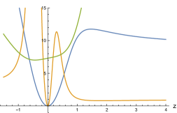
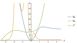
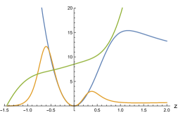
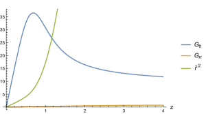
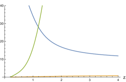
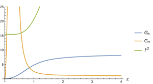
Figure 1: Graphs of the metric $G_{tt}$, $G_{\tilde{r}\tilde{r}}$ and $\tilde{r}^{2}$. We set $c_{3}=0.15$, $c_{0}=0.4$ and $\rho_{0}=3$. The top-left, top-right, center-left, center-right, bottom-left and bottom-right plots are of $c_{1}=-6$, $-4.4$, $-2.8$, $-1.47\cdots$, $-1.4$ and $8$, respectively. The center-right graph with $c_{1}=-1.47\cdots$ is a special case in which $c_{4}=0$. Note that some of the plots show behavior in $z<0$ though such a region is not physically meaningful.

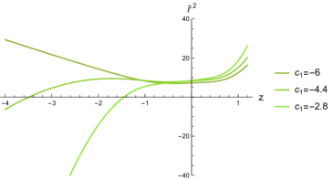
Figure 2: Three types of behaviors of $\tilde{r}^{2}$.

Asymptotic behavior.

The long-distance asymptotics of the metric is obtained most easily by recalling that using $E\sim r^{-3}\sim S$ (4.39), (4.41). Therefore

$$ds^{2}_{G} =\rho^{2}\Big{(}-A^{2}dt^{2}+B^{2}dr^{2}+2rBEdtdr+B^{2}r^{2}d\Omega^{2}\Big{)}\ +O(r^{-4})\ .$$ (5.10)

By redefining $t\to t+\psi^{\prime}(r)$ and using $B=b_{0}+O(r^{-4})$ (4.29), we obtain

$$ds^{2}_{G} =\rho^{2}\Big{(}-A^{2}dt^{2}+b_{0}^{2}(dr^{2}+r^{2}d\Omega^{2})\Big{)}\ +O(r^{-4})\ .$$ (5.11)

Moreover, (4.37) and (4.40) give

$$\rho^{2}A =\sqrt{c_{e}c_{1}}+O(r^{-4}).$$ (5.12)

Therefore the metric has the asymptotic form

$$ds^{2}_{G} =\sqrt{c_{e}c_{1}}\left(-Adt^{2}+\frac{b_{0}^{2}}{A}(dr^{2}+r^{2}d\Omega^{2})\right)+O(r^{-4}),$$ (5.13)

where

$$\frac{1}{A}=\frac{1}{a_{0}}\Big{(}1+\frac{2M}{r}\Big{)}+O(r^{-4})$$ (5.14)

due to (4.37), with mass parameter

$$M=\frac{c_{e}}{2|c_{e}|}\sqrt{\frac{c_{e}}{c_{1}}}\frac{a_{0}c_{0}}{b_{0}}\ .$$ (5.15)

This has the same structure as the simple solution (3.3) found in [8], and reproduces the linearized Schwarzschild metric with mass $M$. Note that we have to choose $c_{e}c_{0}>0$ in order to describe a positive mass.

We can compare the metric with the standard Eddington-Robertson-Schiff parameters

$$ds_{SS}^{2}=-\Big{(}1-\frac{2M}{r}+2\beta\frac{M^{2}}{r^{2}}+...\Big{)}dt^{2}+\Big{(}1+2\gamma\frac{M}{r}+...\Big{)}(dr^{2}+r^{2}d\Omega^{2}),$$ (5.16)

which in GR take the values $\beta=\gamma=1$, while the present solution corresponds to $\gamma=1$ but $\beta=2$. This means that some of the solar system precision test are not satisfied. However, this is not surprising since we have not taken into account the Einstein-Hilbert term, which is induced in the quantum effective action at one loop [9]. Since the E-H action has two extra derivatives compared with the bare matrix model action, it is plausible that the induced E-H action will dominate for short distances, while the present solution of the classical matrix model should dominate at (very) long distances. Then the above metric should perhaps be compared with the metric on galactic scales rather than solar system scales, and the above deviation from Ricci flatness might be compatible with the observation of galactic rotation curves. This will be briefly discussed in section 5.3.

5.2 The $E=0$ branch

For $E=0$, the effective metric (5.1) takes the form

$$ds^{2}_{G} =\rho^{2}\left(-A^{2}dt^{2}+b_{0}^{2}dr^{2}+\left(b_{0}^{2}+\frac{s_{0}^{2}}{r^{4}}\right)r^{2}d\Omega^{2}\right)$$

$$=\tilde{c}_{\rho}\Big{(}-\frac{A}{\sqrt{b_{0}^{2}+s_{0}^{2}r^{-4}}}dt^{2}+\frac{b_{0}^{2}}{A\sqrt{b_{0}^{2}+s_{0}^{2}r^{-4}}}\frac{d\tilde{r}^{2}}{(\tilde{r}^{\prime})^{2}}+\tilde{r}^{2}d\Omega^{2}\Big{)}\ ,$$ (5.17)

using (4.46) and (4.48). Here $A$ is given explicitly by (4.54), and we introduced again the effective radial variable $\tilde{r}$ via

$$\tilde{r}^{2}=\frac{\sqrt{b_{0}^{2}r^{4}+s_{0}^{2}}}{A}\ ,$$ (5.18)

which allows to express $\tilde{r}^{\prime}$ using (4.51) as follows

$$2\tilde{r}\tilde{r}^{\prime} =c_{a1}+\frac{2b_{0}^{2}r^{3}}{A\sqrt{b_{0}^{2}r^{4}+s_{0}^{2}}}\ .$$ (5.19)

Some representative plots are shown in Fig. 3. Again, we set the asymptotic behavior of the metric as $A\to 1$, $B\to 1$, and $\rho\to\rho_{0}=3$. $\tilde{r}^{2}$ is positive and monotonically increasing in the upper graphs with $c_{a1}=1$, $0.14$, but it has a minimum in the lower graph with $c_{a1}=-0.5$. As is the case for $E\neq 0$, $G_{tt}$ diverges as $\tilde{r}$ approaches zero, and $G_{\tilde{r}\tilde{r}}$ diverges as the first derivative of $\tilde{r}^{2}$ approaches zero. $G_{tt}$ and $G_{\tilde{r}\tilde{r}}$ approach $1$ at large $r$.

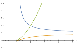
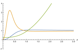
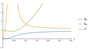
Figure 3: Graphs of the metric $G_{tt}/\tilde{c}_{\rho}$, $G_{\tilde{r}\tilde{r}}/\tilde{c}_{\rho}$ and $\tilde{r}^{2}$. We set $s_{0}=0.4$ and $\rho_{0}=3$. The top-left, top-right and bottom plots are of $c_{a1}=1$, $0.14$ and $-0.5$, respectively.

Asymptotic behavior.

The long-distance asymptotics of this metric is given by

$$ds^{2}_{G} =\rho^{2}A\Big{(}-Adt^{2}+\frac{b_{0}^{2}}{A}(dr^{2}+r^{2}d\Omega^{2})\Big{)}+O(r^{-4})\ .$$ (5.20)

Using (4.52) and (4.54) we obtain

$$\frac{1}{A} =\tilde{c}_{a2}\left(1+\frac{2M}{r}\right)+O(r^{-4})\ ,$$

$$\rho^{2}A =\frac{\tilde{c}_{\rho}}{b_{0}}\ +O(r^{-4})\ ,$$ (5.21)

where

$$\tilde{c}_{a2}=\left\{\begin{array}[]{ll}c_{a2}&\text{; }s_{0}=0\\ c_{a2}+c_{a1}\frac{\Gamma(\frac{1}{4})\Gamma(\frac{5}{4})}{\sqrt{\pi b_{0}|s_{0}|}}&\text{; }s_{0}\neq 0\end{array}\right.$$ (5.24)

$$M=-\frac{c_{a1}}{2\tilde{c}_{a2}b_{0}}\ ,$$ (5.25)

where the terms of $O(r^{-4})$ is absent if $s_{0}=0$. This has again the same structure as the simple solution (3.3) [8] up to $O(r^{-4})$, which deviates from Ricci-flat at the nonlinear level.

5.3 Rotation curves

We expect that the IR regime of the classical computation is more trustworthy than the short-distance regime, where the quantum effects (such as an induced Einstein-Hilbert action [9]) may be important. It is therefore interesting to consider the rotation velocities of circular orbits in these metrics in the large $r$ regime. The question is if this may be similar to the rotation curves $v(r)$ observed in galaxies, whose well-known deviation from GR is usually attributed to dark matter.

In the non-relativistic linearized approximation, the effective (Newtonian) gravitational potential $V(r)$ is given by

$$G_{tt}=-(1+V(r))\ .$$ (5.26)

The equation of motion for a stationary circular orbit is

$$m\frac{v^{2}(r)}{r}=mV^{\prime}(r),\qquad v(r)=\sqrt{rV^{\prime}(r)}$$ (5.27)

(assuming that $r$ is the effective distance). For a central mass in Newtonian gravity, the potential $V(r)=-\frac{2M}{r}$ leads to

$$v(r)\sim\sqrt{\frac{2M}{r}}\ .$$ (5.28)

Now consider the present solution. We have seen that in the long-distance regime $r\to\infty$, the metric has the universal form

$$ds^{2}_{G} \sim-Adt^{2}+\frac{1}{A}(dr^{2}+r^{2}d\Omega^{2})\ +O(r^{-4})$$ (5.29)

up to an overall factor, where

$$\frac{1}{A}=1+\frac{2M}{r}\ +O(r^{-4})\ .$$ (5.30)

Here we set $a_{0}=b_{0}=1$. Then

$$V(r)\sim\frac{1}{1+\frac{2M}{r}}-1=-\frac{2M}{r+2M}.$$ (5.31)

Then we obtain

$$v(r)=\sqrt{\frac{2Mr}{(r+2M)^{2}}}=\sqrt{2M}\frac{\sqrt{r}}{r+2M}.$$ (5.32)

For $r\gg M$, this reproduces the Newtonian $v(r)\sim\sqrt{r^{-1}}$, as it must. However in the regime $r\sim 2M$, the rotation curve is indeed approximately flat, cf. Fig. 4. Of course for aspherical rotating objects, the resulting rotation curve would look somewhat different, and presumably stretched in the rotation plane.

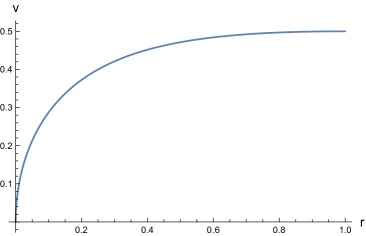
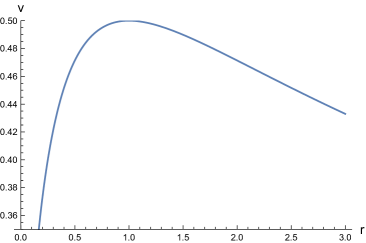
Figure 4: A rotation curve $v(r)$ arising from (5.32), with different truncation in $r$. $M$ is set to $1/2$.

Zooming into the appropriate regime, this may indeed looks like a flat rotation curve. At shorter distances, more pronounced and localized feature may arise e.g. from a non-vanishing axion.

It is amusing to compute the hypothetical mass distribution $M_{N}(r)$ of “dark matter” which would result in the same rotation curve in Newtonian gravity. This is given by

$$M_{N}(r)=M\frac{r^{2}}{(r+2M)^{2}}\ ,$$ (5.33)

where

$$v(r)=\sqrt{\frac{2M_{N}(r)}{r}}\ .$$ (5.34)

This seems not entirely unreasonable.

Note that there is no hidden Newton constant in the potential (5.31), and there is a priori no reason to expect that $M=G_{N}m$ where $m$ is the physical mass in the center; rather, this long-range “tail” of the gravitational potential may be related to $m$ in some other, indirect way. The maximum of the velocity function (5.32) is at

$$r_{M}=2M\ ,$$ (5.35)

where $V(r_{M})=-\frac{1}{2}$. Hence $r_{M}$ is in a regime where the metric is significantly different from its asymptotic value $V(\infty)=0$. This corresponds to the strong gravity regime with associated redshift $\frac{1}{2}$, which is completely unrealistic for galaxies. Therefore this simple picture does not work. A more complete and perhaps realistic analysis would require incorporating the induced Einstein-Hilbert action into the present model. Then it is conceivable that a similar effect arises from a cross-over between the Einstein-Hilbert regime at short scales and the matrix regime at longer distances. However, this would require a more sophisticated analysis. The main point here is that the matrix model framework admits vacuum geometries which deviate from Ricci-flatness at large scales.

5.4 The effective energy-momentum tensor

We can now compute explicitly the various contributions to the effective energy-momentum tensor in the effective Einstein equations arising from the semi-classical matrix model [7]:

$${\cal R}_{\mu\nu}-\frac{1}{2}G_{\mu\nu}{\cal R}={\bf T}_{\mu\nu}\ .$$ (5.36)

Here ${\cal R}_{\mu\nu}$ and ${\cal R}$ are the Ricci tensor and the scalar curvature of the effective metric $G_{\mu\nu}$, respectively, and the energy-momentum tensor is

$${\bf T}_{\mu\nu} ={\bf T}_{\mu\nu}[E^{\dot{\alpha}}]+{\bf T}_{\mu\nu}[\rho]+{\bf T}_{\mu\nu}[\tilde{\rho}]-\rho^{-2}m^{2}G_{\mu\nu}\ .$$ (5.37)

The contributions from the dilaton $\rho$, the axion $\tilde{\rho}$ and the frame $E^{\dot{\alpha}}$ are

$${\bf T}_{\mu\nu}[\rho] =2\rho^{-2}\Big{(}\partial_{\mu}\rho\partial_{\nu}\rho-\frac{1}{2}G_{\mu\nu}G^{\sigma\sigma^{\prime}}\partial_{\sigma}\rho\partial_{\sigma^{\prime}}\rho\Big{)}\ ,$$ (5.38)

$${\bf T}_{\mu\nu}[\tilde{\rho}] =\frac{1}{2}\rho^{-4}\Big{(}\partial_{\mu}\tilde{\rho}\partial_{\nu}\tilde{\rho}-\frac{1}{2}G_{\mu\nu}G^{\sigma\sigma^{\prime}}\partial_{\sigma}\tilde{\rho}\partial_{\sigma^{\prime}}\tilde{\rho}\Big{)}\ ,$$ (5.39)

$${\bf T}_{\mu\nu}[E^{\dot{\alpha}}] =\rho^{2}\Big{(}-\tensor{T}{{}_{\mu}{}_{\rho}^{\sigma}}\tensor{T}{{}_{\nu}{}_{\rho^{\prime}}{}_{\sigma}}G^{\rho\rho^{\prime}}+\frac{1}{4}G_{\mu\nu}\tensor{T}{{}_{\rho}{}_{\sigma}^{\kappa}}\tensor{T}{{}_{\rho^{\prime}}{}_{\sigma^{\prime}}{}_{\kappa}}G^{\rho\rho^{\prime}}G^{\sigma\sigma^{\prime}}\Big{)}\ .$$ (5.40)

Axion.

Consider first the axion, which is non-vanishing only for $E\neq 0$. Under the static-axion condition (3.20), the axion (3.22) becomes

$$\tilde{T}_{r}=\frac{4r\rho^{4}|A|ES}{c_{e}c_{1}}\frac{1}{|B|}=\sqrt{-\frac{c_{2}}{c_{e}^{3}}}\frac{4r^{4}\rho^{4}E^{2}S}{c_{1}|B|^{2c_{3}+1}}\ ,$$ (5.41)

using the integral of motion (4.8) and then (4.17). Therefore, substituting $S$ with (4.27), we have

$$\tilde{T}_{r}=\rho^{-2}\partial_{r}\tilde{\rho} =\pm 4c_{e}\sqrt{-c_{1}c_{2}c_{3}}\frac{r^{3}|B|^{2(1-c_{3})}}{(c_{3}c_{e}+c_{1}\,r^{4}B^{4})^{2}}\ \sim r^{-5}\ ,$$ (5.42)

where the sign is plus if $S>0$ and minus if $S<0$. This could become singular if

$$-c_{3}c_{e}=c_{1}r^{4}B^{4},$$ (5.43)

which may happen for $c_{3}=0$ and is associated with a singularity of $(\ln B)^{\prime}$ (see (4.14)); however, this singularity does not appear because $\tilde{T}_{r}$ is zero for $c_{3}=0$.

Dilaton.

For $E\neq 0$, we have

$$(\ln\rho)^{\prime} =\frac{1}{r}-\frac{1}{c_{e}}\frac{c_{1}r^{4}B^{4}-c_{e}}{c_{1}r^{2}B^{2}}E\rho^{2}-\frac{2}{c_{1}c_{e}}r(E\rho^{2})^{2}-\frac{c_{0}}{2}rBE\ ,$$ (5.44)

using (4.5) and (4.8). We then can consider the asymptotic expansion

$$(\ln\rho)^{\prime} \sim\frac{1}{r}-\frac{b_{0}^{2}}{c_{e}}r^{2}E\rho^{2}-\frac{2}{c_{1}c_{e}}r(E\rho^{2})^{2}-\frac{c_{0}b_{0}}{2}rE$$

$$=\Big{(}1-\frac{b_{0}^{2}}{c_{e}}(r^{3}E\rho^{2})\Big{)}\frac{1}{r}-\frac{c_{0}b_{0}}{2}(r^{3}E)\frac{1}{r^{2}}-\frac{2}{c_{1}c_{e}}(r^{3}E)^{2}\rho^{4}\frac{1}{r^{5}}$$

$$=-\frac{c_{0}c_{e}}{2b_{0}}\rho^{-2}\frac{1}{r^{2}}+O(r^{-5})\ ,$$ (5.45)

using

$$\frac{b_{0}^{2}}{c_{e}}r^{3}E\rho^{2}\sim 1+O(r^{-4})\ ,$$ (5.46)

which can be obtained from (4.39) and (4.40). But this leads to

$${\cal R}=-G^{\mu\nu}({\bf T}_{\mu\nu}[\rho]+{\bf T}_{\mu\nu}[\tilde{\rho}])\sim r^{-4}\neq 0\ .$$ (5.47)

The $\rho$ contribution clearly dominates and cannot be removed.

Metric and the energy-momentum tensors.

The graphical relationship between the metric, $\tilde{r}$ and the traces of the energy-momentum tensors is shown in Fig. 5 for $E\neq 0$ and in Fig. 6 for $E=0$ (with $S\neq 0$). One can see that the traces of the energy-momentum tensor of the dilaton have poles. Interestingly, in both cases $E\neq 0$ and $E=0$, the scalar curvature does not diverge at the points where $G_{\tilde{r}\tilde{r}}$ diverges. Moreover, we observe the scalar curvature diverges if $G_{tt}$ is infinity or $r$ is zero.

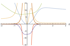
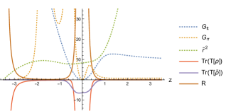
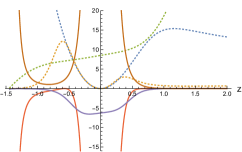
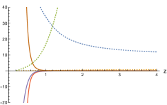
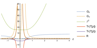
Figure 5: Graphs of the traces of the energy-momentum tensors and the scalar curvature with the metric $G_{tt}$, $G_{\tilde{r}\tilde{r}}$ and $\tilde{r}^{2}$ for $E\neq 0$. We set $c_{3}=0.15$, $c_{0}=0.4$ and $\rho_{0}=3$. The top-left, top-right, center-left, center-right, bottom-left and bottom-right plots are of $c_{1}=-6$, $-4.4$, $-2.8$, $-1.47\cdots$, $-1.4$ and $8$, respectively. Note that they correspond to the ones in Fig. 1. In contrast to Fig. 1, the metric and $\tilde{r}^{2}$ are plotted by dashed curves here.

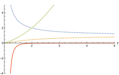
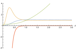
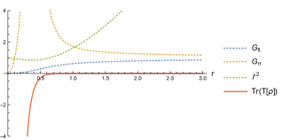
Figure 6: Graphs of the trace of the dilaton’s energy-momentum tensor with the metric $G_{tt}/\tilde{c}_{\rho}$, $G_{\tilde{r}\tilde{r}}/\tilde{c}_{\rho}$ and $\tilde{r}^{2}$ for $E=0$. We set $s_{0}=0.4$ and $\rho_{0}=3$. The top-left, top-right, bottom-left and bottom-right plots are of $c_{a1}=1$, $0.14$, $-0.5$, respectively. The scalar curvature is not plotted because $\mathcal{R}=-\mbox{Tr}(\mathbf{T}[\rho])$. Note also that these graphs correspond to the ones in Fig. 3. Again, in contrast to Fig. 3, the metric and $\tilde{r}^{2}$ are plotted by dashed curves here.

6 Discussion and outlook

We derived and classified general $SO(3)$-symmetric static solutions to the matrix-model equations of motion written in terms of the frame of $\mathcal{M}^{3,1}$. We identify two different classes of solutions: one without axion for $E=0$ in our ansatz, and one including an axion for $E\neq 0$. We imposed a natural condition (3.20), in which the axion is also static. The behavior of the solutions has several remarkable features.

Firstly, the asymptotic behavior of the general solutions is the same as the previously found special solution (3.3), for sufficiently large $r$. This suggests that the special solution well represents the general solutions to the equations of motion, which include further contributions due to the axion and dilaton at shorter distances.

Secondly in the $E\neq 0$ case, it is remarkable that there is a parameter region where the effective metric is double-valued in the effective radius squared $\tilde{r}^{2}$. More precisely, in such a solution there are two values of $z$ corresponding to a value of $\tilde{r}^{2}$, so that there are two corresponding values of the other elements of the metric. The metric has a singularity at the minimal $\tilde{r}^{2}$. This can be viewed as a wormhole-like solution. Since there is no symmetry of flipping $z$ around the minimum of $\tilde{r}^{2}$, it turned out the behaviors of the two sides of the metric are entirely different in general.

Finally, we found that the Schwarzschild solution is not contained in the general solutions, though the asymptotic behavior of the general metric reproduces the linearized Schwarzschild metric. Although this sounds like an unwanted result, we can expect to recover such a solution upon taking into account the Einstein-Hilbert term, which is induced by one-loop effects [9]. In particular, it is interesting that the origin of the (asymptotic) mass of the present solutions is not some singular matter localized at the center, but a new type of “vacuum energy” due to dilaton, axion, and the noncommutative frame itself. Therefore the solutions obtained in this paper should be understood as solutions to the pre-gravity theory arising on classical brane solutions, and their full significance will only be understood upon taking into account the induced Einstein-Hilbert term. The results and techniques developed here should allow to study also solutions of such a combined action. This is certainly the most important open problem, which is postponed for future work.

There are clearly many further directions for follow-up work. For example, we studied only static solutions in this paper. Since the classical solutions obtained without the Einstein-Hilbert term are expected to describe spacetime in the cosmological regime, it will be intriguing to investigate more general solutions with cosmic time evolution. Establishing a relation of such cosmic solutions to numerical attempts to realise cosmic time evolution from the matrix model, e.g. [12, 13], would significantly improve our understanding of the matrix model and the universe. On a more technical level, we have provided a partial answer to the problem of reconstructing matrix configurations for a given frame. A more complete treatment of this problem and of possible higher-spin contributions should be given elsewhere.

Appendix A Reconstruction of the frame

In this paper, we have solved the equations of motion for the frame $\tensor{E}{{}_{\dot{\alpha}}^{\mu}}$. However, it remains to be shown that such frames can indeed arise as configurations in the semi-classical matrix model, i.e. via Poisson brackets (LABEL:frame-Poisson)

$$\{Z_{\dot{\alpha}},x^{\mu}\}=\tensor{E}{{}_{\dot{\alpha}}^{\mu}}\qquad\in{\cal C}^{0}$$ (A.1)

in terms of the basic matrices $Z_{\dot{\alpha}}$. For the solution found in [8], that question was settled directly by constructing suitable $Z_{\dot{\alpha}}$. This was possible, but required an infinite tower of higher-spin contributions to $Z_{\dot{\alpha}}$.

Here we want to address this question more generally: Given any (spin 0 valued) frame $\tensor{E}{{}_{\dot{\alpha}}^{\mu}}\in{\cal C}^{0}$ which satisfies the divergence constraint $\partial_{\nu}\big{(}\rho_{M}\tensor{E}{{}^{\nu}}\big{)}=0$ (2.17), are there always generators (“potentials”) $Z_{\dot{\alpha}}$ such that (A.1) holds?

We can provide a partial answer to this question: For any divergence-free frame $\tensor{E}{{}_{\dot{\alpha}}^{\mu}}\in{\cal C}^{0}$, we can construct generators $Z_{\dot{\alpha}}\in{\cal C}^{1}$ such that $[\{Z_{\dot{\alpha}},x^{\mu}\}]_{0}=\tensor{E}{{}_{\dot{\alpha}}^{\mu}}$ for the projection $[.]_{0}$ on ${\cal C}^{0}$. However, we cannot settle the question if this equation can be satisfied for all higher-spin components for suitable $Z_{\dot{\alpha}}$; this is postponed to future work. Moreover we restrict ourselves to the asymptotic regime, where the wavelengths are much smaller than the cosmic scale. To show this (partial) result, we first establish some results for the fuzzy hyperboloid $H^{4}_{n}$ which is underlying ${\cal M}^{3,1}$.

A.1 Divergence-free vector fields on $H^{4}$ and reconstruction

First we recall some results for the fuzzy hyperboloid $H_{n}^{4}\subset{\mathbb{R}}^{4,1}$ (see (4.9) and (9.9) in [14]):

Lemma A.1.

Given a divergence-free tangential vector field $\phi_{a}\in{\cal C}^{0}$ on $H^{4}$, we have

$$-\{x_{a},\phi^{(1)}\}_{0} =\frac{1}{3}(\Box_{H}-2r^{2})\phi_{a}\ ,\qquad\mbox{where}\ \ \phi^{(1)}=\{x^{a},\phi_{a}\}\$$ (A.2)

where $x^{a}$ are Cartesian coordinates on ${\mathbb{R}}^{4,1}$.

Lemma A.2.

$$(\Box_{H}+2r^{2}s)\{\phi^{(s)},x_{a}\}_{-} =\{\Box_{H}\phi^{(s)},x_{a}\}_{-}$$ (A.3)

$$(\Box_{H}-2r^{2}(s+1))\{\phi^{(s)},x_{a}\}_{+} =\{\Box_{H}\phi^{(s)},x_{a}\}_{+}\$$ (A.4)

for any $\phi^{(s)}\in{\cal C}^{s}$. Here $[]_{\pm}$ denotes the projection on ${\cal C}^{s\pm 1}$.

Now consider the following (possibly $\mathfrak{hs}$-valued) vector fields on $H^{4}$

$$V:=V^{a}\eth_{a},\qquad V^{a}=\{Z,x^{a}\}$$ (A.5)

generated by some $Z\in{\cal C}$, where $\eth_{a}$ is the tangential derivative operator on $H^{4}_{n}$ introduced in [4]. It was shown there that $V$ is always tangential to $H^{4}$ and divergence-free,

$$\eth_{a}V^{a}=0\ .$$ (A.6)

$V$ can be viewed as push-forward of the Hamiltonian vector field $\{Z,.\}$ on ${\mathbb{C}}P^{1,2}$ to $H^{4}$ via the bundle projection. For $Z=Z^{(s)}\in{\cal C}^{s}$, it decomposes into different $\mathfrak{hs}$ components as

$$V^{a}=V^{a}_{(s-1)}+V^{a}_{(s+1)}\qquad{\cal C}^{s-1}\oplus{\cal C}^{s+1}\ .$$ (A.7)

One might hope that all divergence-free $\mathfrak{hs}$-valued vector fields can be written in this form, but this is not possible, by counting degrees of freedom. However for $s=0$, all divergence-free vector fields $V^{a}\in{\cal C}^{0}$ can indeed be obtained in this way for a suitable $Z\in{\cal C}^{1}$, up to $\mathfrak{hs}$ corrections. More precisely, we have the following result:

Lemma A.3.

Given any divergence-free tangential vector field $\eth_{a}V^{a}=0$ on $H^{4}$ with $V^{a}\in{\cal C}^{0}$, there is a unique generator $Z\in{\cal C}^{1}$ such that

$$V^{a}=\{Z,x^{a}\}_{0}\ .$$ (A.8)

This $Z$ is given explicitly by

$$Z:=-3(\Box_{H}-4r^{2})^{-1}\{V^{a},x_{a}\}\qquad\in{\cal C}^{1}\ .$$ (A.9)

Proof.

As pointed out above, the vector field $\{Z,x^{a}\}$ is always divergence-free,

$$\eth_{a}\{Z,x^{a}\}=0\ .$$ (A.10)

The intertwiner result (A.3) implies

$$(\Box_{H}-2r^{2})\{Z^{(1)},x_{a}\}_{-} =\{((\Box_{H}-4r^{2})Z^{(1)},x_{a}\}_{-}$$

$$\{(\Box_{H}-4r^{2})^{-1}Z^{(1)},x_{a}\}_{-} =(\Box_{H}-2r^{2})^{-1}\{Z^{(1)},x_{a}\}_{-}$$ (A.11)

for any $Z^{(1)}\in{\cal C}^{1}$. Therefore

$$\{Z,x^{a}\}_{0} =-3\{(\Box_{H}-4r^{2})^{-1}\{V^{b},x_{b}\},x^{a}\}_{0}=-3(\Box_{H}-2r^{2})^{-1}\{\{V^{b},x_{b}\},x^{a}\}_{0}=V^{a}$$ (A.12)

using Lemma A.1 in the last step. Uniqueness can be seen similarly using the results in [14]. The inverse operators make sense at least for square-integrable functions, because $\Box_{H}-\frac{9}{2}r^{2}$ is positive-definite on $H^{4}$ for unitary irreps (cf. [14]), and $\Box_{H}-4r^{2}$ is positive-definite on unitary modes in ${\cal C}^{1}$.

∎

Now consider the reconstruction problem on $H^{4}_{n}$. Given $V^{a}$, we define

$$Z^{(1)}:=-3(\Box_{H}-4r^{2})^{-1}\{V^{a},x_{a}\}\qquad\in{\cal C}^{1}\$$ (A.13)

which satisfies

$$V^{a}=\{Z^{(1)},x^{a}\}_{0}\$$ (A.14)

as shown above. However, $\{Z^{(1)},x^{a}\}$ contains in general also a spin 2 component

$$V^{(2)a}:=\{Z^{(1)},x^{a}\}_{2}\qquad\in{\cal C}^{2}\ .$$ (A.15)

Noting that $\eth$ respects ${\cal C}^{n}$, this satisfies

$$\eth_{a}V^{(2)a} =0,$$

$$\{V^{(2)a},x_{a}\}_{3} =\{\{Z^{(1)},x^{a}\}_{2},x_{a}\}_{3}=0\$$ (A.16)

since ${\cal C}^{3}$ does not contain any spin 1 mode. The second relation means that we cannot just repeat the above procedure to cancel this. One can show that the only generators $Z\in{\cal C}^{1}$ which do not induce spin 2 components via (A.15) are linear combinations of $\theta^{ab}$.

This means that the reconstruction of vector fields on $H^{4}$ generically leads to extra higher-spin components $V^{(2)a}\in{\cal C}^{2}$ (A.15), which however encode the same information as $V^{a}$. It remains an open question if these can be cancelled by suitable $\mathfrak{hs}$-modifications of $Z$ and possibly $x^{a}$.

A.2 Divergence-free vector fields and reconstruction on ${\cal M}^{3,1}$

Now we recall that ${\cal M}^{3,1}\subset{\mathbb{R}}^{3,1}$ is obtained from $H^{4}\subset{\mathbb{R}}^{4,1}$ via a projection along $x^{4}$. Therefore any vector field $V^{a}$ on $H^{4}$ can be projected to a vector field $V^{\mu}$ on ${\cal M}^{3,1}$ by simply dropping the $V^{4}$ component. In particular, the Hamiltonian vector field $V^{a}=\{Z,x^{a}\}$ is mapped to $V^{\mu}=\{Z,x^{\mu}\}$ in Cartesian coordinates. Conversely, any vector field $V^{\mu}$ on ${\cal M}^{3,1}$ can be lifted to $H^{4}$ by defining

$$V^{4}:=-\frac{1}{x_{4}}x_{\mu}V^{\mu}\ ,$$ (A.17)

which clearly satisfies the tangential relation $V^{a}x_{a}=0$ on $H^{4}$.

It turns out that this correspondence maps divergence-free (${\cal C}^{0}$-valued) vector fields $\eth_{a}V^{a}=0$ on $H^{4}$ to divergence-free vector fields on ${\cal M}^{3,1}$ and vice versa, in the sense that

$$\partial_{\mu}(\rho_{M}V^{\mu})=0,\qquad\rho_{M}=\sinh(\eta)^{-1}\ .$$ (A.18)

This is established in the following result:

Lemma A.4.

Let $V^{a}$ be a (${\cal C}^{0}$-valued, tangential) divergence-free vector field on $H^{4}$. Then its reduction (or push-forward) to ${\cal M}^{3,1}$ satisfies

$$\partial_{\mu}(\rho_{M}V^{\mu})=0\ .$$ (A.19)

Conversely, if $V^{\mu}$ satisfies (A.19) then its lift to $H^{4}$ defined by (A.17) is divergence-free in the sense of (A.6).

Proof.

First we recall the following property of the tangential derivative $\eth$ from (3.65) in [14]

$$\eth^{\mu}x^{\nu} =\eta^{\mu\nu}+\frac{1}{R^{2}}x^{\mu}x^{\nu}\,=\big{(}\partial^{\mu}+\frac{1}{R^{2}}x^{\mu}x^{\sigma}\partial_{\sigma}\big{)}x^{\nu}\ .$$ (A.20)

Therefore we can identify

$$\eth^{\mu}=\partial^{\mu}+\frac{1}{R^{2}}x^{\mu}x^{\sigma}\partial_{\sigma}\qquad\mbox{on}\ \ {\cal C}^{0}\ .$$ (A.21)

Furthermore,

$$\eth^{4}Z =\frac{1}{r^{2}R^{2}}x_{\mu}\{\theta^{4\mu},Z\}=\frac{1}{R}x^{\mu}\{t_{\mu},Z\}=\frac{\sinh(\eta)}{R}x^{\mu}\partial_{\mu}Z$$ (A.22)

for $Z\in{\cal C}^{0}$, since $\theta^{4\mu}=r^{2}{\cal M}^{\mu 4}=r^{2}Rt^{\mu}$. Therefore

$$\eth_{a}V^{a} =\eth_{\mu}V^{\mu}+\eth_{4}V^{4}$$

$$=\big{(}\partial_{\mu}+\frac{1}{R^{2}}x_{\mu}x^{\sigma}\partial_{\sigma}\big{)}V^{\mu}-\frac{\sinh(\eta)}{R^{2}}x^{\nu}\partial_{\nu}(\sinh(\eta)^{-1}x_{\mu}V^{\mu})$$

$$=\sinh(\eta)\partial_{\mu}(\sinh(\eta)^{-1}V^{\mu})\ .$$ (A.23)

∎

Reconstruction of vector fields and frame.

We can now solve the following “reconstruction” problem on ${\cal M}^{3,1}$: Given any ${\cal C}^{0}$-valued divergence-free vector field $V^{\mu}$,

$$\partial_{\mu}(\rho_{M}V^{\mu})=0\ ,$$ (A.24)

there is a generating function $Z\in{\cal C}^{1}$ such that

$$V^{\mu}=\{Z,x^{\mu}\}_{0}\ .$$ (A.25)

This can be obtained by lifting $V^{\mu}$ to a divergence-free vector field $V^{a}$ on $H^{4}$ as in Lemma A.4. Then the result (A.8) on $H^{4}$ states that $V^{a}=\{Z,x^{a}\}_{0}$ for some $Z\in{\cal C}^{1}$, which implies $V^{\mu}=\{Z,x^{\mu}\}_{0}$. Explicitly, this $Z$ is given by

$$Z =-3(\Box_{H}-4r^{2})^{-1}\big{(}\{V^{\mu},x_{\mu}\}+\{V^{4},x_{4}\}\big{)}$$

$$=-3(\Box_{H}-4r^{2})^{-1}\big{(}\{V^{\mu},x_{\mu}\}+\frac{1}{x_{4}}\{x_{4},x_{\mu}V^{\mu}\}\big{)}\ .$$ (A.26)

In particular, for given any classical frame $\tensor{E}{{}_{\alpha}^{\mu}}$ there is a unique $Z_{\alpha}\in{\cal C}^{1}$ such that $\tensor{E}{{}_{\alpha}^{\mu}}=\{Z_{\alpha},x^{\mu}\}_{0}$. E.g. for the cosmic background frame, this gives $E_{\alpha 4}=0$, and we recover

$$Z_{\alpha}=-12(\Box_{H}-4r^{2})^{-1}\{\sinh(\eta),x_{\alpha}\}=t_{\alpha}\ .$$ (A.27)

The generator $Z_{\alpha}\in{\cal C}^{1}$ is uniquely determined by (A.25). This means that the corresponding spin 2 part $\{Z,x^{\mu}\}_{+}\in{\cal C}^{2}$ is also uniquely determined by the vector field. Therefore in general, the reconstructed frame will contain higher spin components. These higher-spin components cancel upon averaging over $S^{2}_{n}$ in the linearized theory, but not in the non-linear regime. Since the $\mathfrak{hs}$ components of the generators $Z_{\alpha}$ in ${\cal C}^{s}$ for $s\geq 2$ are undetermined, it is plausible that these can be adjusted such that the unwanted higher-spin components of the frame cancel (possibly upon redefining $x^{\mu}$), as in the rotationally invariant solution in [8].

In any case, these $\mathfrak{hs}$ components encode the same vector field as the underlying spin $0$ component of the frame, cf. (D.18) in [10], since both are encoded in $Z_{\alpha}\in{\cal C}^{1}$. This means that in a contraction of the frame (such as the metric) or of the torsion (such as in the Einstein-Hilbert action), the averaged contribution of these $\mathfrak{hs}$ components over the internal $S^{2}_{n}$ should be similar to the spin 0 component; however this needs to be established in detail elsewhere. Once this is understood, one may also try to relate our solutions with analogous solutions [15, 16] obtained in Vasiliev higher spin theory, notably after taking into account the induced Einstein-Hilbert term [9]. All this remains to be studied in more detail elsewhere.

Appendix B Deriving the equation of motion

Let us briefly review how to derive the equation of motion (2.23).

We start from the bosonic part of the matrix-model action (2.1):

$$S_{\text{bos}}[Z]=\mbox{Tr}\left([Z^{\dot{\alpha}},Z^{\dot{\beta}}][Z_{\dot{\alpha}},Z_{\dot{\beta}}]+2m^{2}Z_{\dot{\alpha}}Z^{\dot{\alpha}}\right).$$ (B.1)

The equation of motion of the matrix model is

$$[Z^{\dot{\beta}},[Z_{\dot{\beta}},Z_{\dot{\alpha}}]]-m^{2}Z_{\dot{\alpha}}=0,$$ (B.2)

which reduces to

$$\{Z^{\dot{\beta}},\{Z_{\dot{\beta}},Z_{\dot{\alpha}}\}\}+m^{2}Z_{\dot{\alpha}}=0,$$ (B.3)

in the semi-classical limit, where the endomorphism algebra $\mathrm{End}({\cal H})$ becomes a commutative algebra of functions.

This equation of motion can be rewritten via the frame by a simple computation. Let us first denote the Hamiltonian vector field for a field $M$ on the manifold where the functions reside in the semi-classical limit, by

$$\mathcal{P}(M)f:=i\{M,f\}.$$ (B.4)

This satisfies

$$[\mathcal{P}(M_{1}),\mathcal{P}(M_{2})]=\mathcal{P}(i\{M_{1},M_{2}\}),$$ (B.5)

and therefore for $Z_{\dot{\alpha}}$,

$$[\mathcal{P}(Z^{\dot{\beta}}),[\mathcal{P}(Z_{\dot{\beta}}),\mathcal{P}(Z_{\dot{\alpha}})]]=\mathcal{P}(-\{Z^{\dot{\beta}},\{Z_{\dot{\beta}},Z_{\dot{\alpha}}\}\}),$$ (B.6)

where $[\ast,\ast\,]$ is the usual commutator. Thus the equation of motion (B.3) can be computed by

$$[\mathcal{P}(Z^{\dot{\beta}}),[\mathcal{P}(Z_{\dot{\beta}}),\mathcal{P}(Z_{\dot{\alpha}})]]=m^{2}\mathcal{P}(Z_{\dot{\alpha}}).$$ (B.7)

The action of $Z_{\dot{\alpha}}$ on a function can be written by a Weitzenböck connection $\nabla_{\dot{\alpha}}$ if $\tensor{E}{{}_{\dot{\alpha}}^{\mu}}$ is a set of globally defined linear independent frame fields, i.e. $\mathcal{M}^{3,1}$ is parallelizable. The relation between them is $\mathcal{P}(Z_{\dot{\alpha}})=i\nabla_{\dot{\alpha}}$ since

$$\mathcal{P}(Z_{\dot{\alpha}})f=i\{Z_{\dot{\alpha}},f\}=i\tensor{E}{{}_{\dot{\alpha}}^{M}}\partial_{M}f=i\nabla_{\dot{\alpha}}f.$$ (B.8)

It acts as $\nabla_{\dot{\alpha}}=\tensor{E}{{}_{\dot{\alpha}}^{\mu}}\partial_{\mu}$ without a spin-connection term on fields without any general coordinate indices while it acts on contravariant vector fields as $\nabla_{\mu}V^{\nu}=\partial_{\mu}V^{\nu}+\tensor{\Gamma}{{}_{\mu\rho}^{\nu}}V^{\rho}$.

Then the equation of motion is written as a relation for operators:

$$[\nabla^{\dot{\beta}},[\nabla_{\dot{\beta}},\nabla_{\dot{\alpha}}]]=-m^{2}\nabla_{\dot{\alpha}}\ .$$ (B.9)

Since the commutator of the covariant derivatives satisfies

$$[\nabla_{\dot{\alpha}},\nabla_{\dot{\beta}}]=-\tensor{T}{{}_{\dot{\alpha}\dot{\beta}}^{\dot{\gamma}}}\nabla_{\dot{\gamma}},$$ (B.10)

where $\tensor{T}{{}_{\dot{\alpha}\dot{\beta}}^{\dot{\gamma}}}=\tensor{E}{{}_{\dot{\alpha}}^{\mu}}\tensor{E}{{}_{\dot{\beta}}^{\nu}}\tensor{T}{{}_{\mu\nu}^{\dot{\gamma}}}$ is the torsion for the Weitzenböck connection, the equation of motion becomes

$$\nabla_{\dot{\beta}}\tensor{T}{{}^{\dot{\beta}}_{\dot{\alpha}}{}^{\dot{\gamma}}}+\tensor{T}{{}_{\dot{\alpha}\dot{\beta}}^{\dot{\delta}}}\tensor{T}{{}^{\dot{\beta}}_{\dot{\delta}}{}^{\dot{\gamma}}}-m^{2}\delta_{\dot{\alpha}}^{\dot{\gamma}}=0,$$

or partially in terms of the general coordinate indices,

$$\nabla_{\mu}(\gamma^{\mu\nu}\tensor{T}{{}_{\nu\rho}^{\dot{\alpha}}})+\tensor{T}{{}_{\rho\mu}{}_{\nu}}\tensor{T}{{}^{\mu\nu}{}^{\dot{\alpha}}}-m^{2}\tensor{E}{{}^{\dot{\alpha}}_{\rho}}=0.$$ (B.11)

This is the equation derived in [7], where $T^{\mu\nu\dot{\alpha}}=\gamma^{\mu\mu^{\prime}}\gamma^{\nu\nu^{\prime}}\tensor{T}{{}_{\mu^{\prime}\nu^{\prime}}^{\dot{\alpha}}}$.

Let us then rewrite the above equation of motion in terms of the Levi-Civita connection. The relation of the Weitzenböck connection with the Levi-Civita connection is

$$\tensor{\Gamma}{{}_{\mu\nu}^{\rho}} =-\tensor{E}{{}^{\dot{\alpha}}_{\nu}}\partial_{\mu}\tensor{E}{{}_{\dot{\alpha}}^{\rho}}=\tensor{\Gamma}{{}^{(\gamma)}_{\mu\nu}{}^{\rho}}+\tensor{K}{{}_{\mu\nu}^{\rho}}$$

$$=\tensor{\Gamma}{{}^{(G)}_{\mu\nu}{}^{\rho}}+\tensor{K}{{}_{\mu\nu}^{\rho}}-\rho^{-1}\left(\delta_{\nu}^{\rho}\partial_{\mu}\rho+\delta_{\mu}^{\rho}\partial_{\nu}\rho-\gamma_{\mu\nu}\gamma^{\sigma\rho}\partial_{\sigma}\rho\right),$$ (B.12)

where $\tensor{\Gamma}{{}^{(\gamma)}_{\mu\nu}{}^{\rho}}$ and $\tensor{\Gamma}{{}^{(G)}_{\mu\nu}{}^{\rho}}$ are the Levi-Civita connections associated with $\gamma_{\mu\nu}$ and $G_{\mu\nu}$, respectively, and $\tensor{K}{{}_{\mu\nu}^{\rho}}$ is the contorsion of the Weitzenböck connection, which is also interpreted as the spin connection constructed from $\tensor{\Gamma}{{}^{(\gamma)}_{\mu\nu}{}^{\rho}}$ via $\tensor{K}{{}_{\mu}^{\dot{\alpha}\dot{\beta}}}=-\tensor{E}{{}^{\dot{\beta}}_{\rho}}\nabla^{(\gamma)}_{\mu}\tensor{E}{{}^{\dot{\alpha}\rho}}$. We denote the covariant derivative associated with $\gamma_{\mu\nu}$ and $G_{\mu\nu}$ by $\nabla^{(\gamma)}_{\mu}$ and $\nabla^{(G)}_{\mu}$, respectively. Substituting the Weitzenböck connection with (B.12) and using the relation $\tensor{T}{{}_{\mu\nu}^{\rho}}=\tensor{K}{{}_{\mu\nu}^{\rho}}-\tensor{K}{{}_{\nu\mu}^{\rho}}$, one obtains

$$\nabla^{(G)}_{\mu}(\gamma^{\mu\nu}\tensor{T}{{}_{\nu}{}_{\rho}^{\dot{\alpha}}})+\frac{1}{2}(\tensor{T}{{}_{\mu\nu\rho}}+\tensor{T}{{}_{\nu\rho\mu}}+\tensor{T}{{}_{\rho\mu\nu}})\tensor{T}{{}^{\mu\nu\dot{\alpha}}}$$

$$\hskip 80.0pt+\gamma^{\mu\nu}\tensor{T}{{}_{\sigma\mu}^{\sigma}}\tensor{T}{{}_{\nu}{}_{\rho}^{\dot{\alpha}}}-(\delta_{\sigma}^{\sigma}-2)\gamma^{\mu\nu}\rho^{-1}\partial_{\mu}\rho\,\tensor{T}{{}_{\nu}{}_{\rho}^{\dot{\alpha}}}-m^{2}\tensor{E}{{}^{\dot{\alpha}}_{\rho}}=0.$$ (B.13)

The Jacobi identity for $\theta^{\mu\nu}$, which reduces to the identity $\partial_{\nu}(\rho_{M}\theta^{\mu\nu})=0$, results in the divergence constraint (2.17). Namely, one can show that the frame satisfies [7]

$$\partial_{\mu}(\sqrt{|G|}\rho^{-2}\tensor{E}{{}_{\dot{\alpha}}^{\mu}})=\partial_{\mu}(\rho_{M}\tensor{E}{{}_{\dot{\alpha}}^{\mu}})=-\partial_{\mu}(\rho_{M}\theta^{\mu\nu}\partial_{\nu}Z_{\dot{\alpha}})=-\partial_{\mu}(\rho_{M}\theta^{\mu\nu})\partial_{\nu}Z_{\dot{\alpha}}=0,$$

and hence $\tensor{E}{{}^{\dot{\alpha}}_{\mu}}\partial_{\nu}\tensor{E}{{}_{\dot{\alpha}}^{\nu}}=-\partial_{\mu}\ln\rho_{M}$. Therefore, (2.22) holds:

$$\tensor{K}{{}_{\sigma\mu}^{\sigma}}=\tensor{T}{{}_{\sigma\mu}^{\sigma}}=-\tensor{E}{{}^{\dot{\alpha}}_{\mu}}\partial_{\nu}\tensor{E}{{}_{\dot{\alpha}}^{\nu}}+\tensor{E}{{}^{\dot{\alpha}}_{\nu}}\partial_{\mu}\tensor{E}{{}_{\dot{\alpha}}^{\nu}}=\partial_{\mu}\ln\left[\frac{\rho_{M}}{\sqrt{|\gamma|}}\right]=\frac{2}{\rho}\partial_{\mu}\rho.$$

By plugging this equation into the equation of motion (B.13), one reaches

$$\nabla^{(G)}_{\mu}(\gamma^{\mu\nu}\tensor{T}{{}_{\nu}{}_{\rho}^{\dot{\alpha}}})+\frac{1}{2}(\tensor{T}{{}_{\mu\nu\rho}}+\tensor{T}{{}_{\nu\rho\mu}}+\tensor{T}{{}_{\rho\mu\nu}})\tensor{T}{{}^{\mu\nu\dot{\alpha}}}-m^{2}\tensor{E}{{}^{\dot{\alpha}}_{\rho}}=0.$$ (B.14)

Finally, the following relation

$$\rho^{2}\sqrt{|G|}^{-1}\varepsilon^{\mu\nu\rho^{\prime}\sigma}G_{\rho\rho^{\prime}}\tilde{T}_{\sigma}\,=-\gamma^{\mu\mu^{\prime}}\gamma^{\nu\nu^{\prime}}(\tensor{T}{{}_{\mu^{\prime}\nu^{\prime}\rho}}+\tensor{T}{{}_{\nu^{\prime}\rho\mu^{\prime}}}+\tensor{T}{{}_{\rho\mu^{\prime}\nu^{\prime}}})$$ (B.15)

leads us to the form of the equation of motion (2.23).

References

- [1] N. Ishibashi, H. Kawai, Y. Kitazawa and A. Tsuchiya, A Large N reduced model as superstring, Nucl. Phys. B498 (1997) 467 [hep-th/9612115].
- [2] T. Banks, W. Fischler, S. H. Shenker and L. Susskind, M theory as a matrix model: A Conjecture, Phys. Rev. D55 (1997) 5112 [hep-th/9610043].
- [3] J. Castelino, S. Lee and W. Taylor, Longitudinal five-branes as four spheres in matrix theory, Nucl. Phys. B526 (1998) 334 [hep-th/9712105].
- [4] M. Sperling and H. C. Steinacker, Covariant cosmological quantum space-time, higher-spin and gravity in the IKKT matrix model, JHEP 07 (2019) 010 [1901.03522].
- [5] H. C. Steinacker, Cosmological space-times with resolved Big Bang in Yang-Mills matrix models, JHEP 02 (2018) 033 [1709.10480].
- [6] H. C. Steinacker, Quantized open FRW cosmology from Yang-Mills matrix models, Phys. Lett. B782 (2017) 2018 [1710.11495].
- [7] H. C. Steinacker, Higher-spin gravity and torsion on quantized space-time in matrix models, JHEP 04 (2020) 111 [2002.02742].
- [8] S. Fredenhagen and H. C. Steinacker, Exploring the gravity sector of emergent higher-spin gravity: effective action and a solution, 2101.07297.
- [9] H. C. Steinacker, Gravity as a Quantum Effect on Quantum Space-Time, 2110.03936.
- [10] M. Sperling and H. C. Steinacker, The fuzzy 4-hyperboloid and higher-spin in Yang–Mills matrix models, Nucl. Phys. B941 (2019) 680 [1806.05907].
- [11] H. C. Steinacker, On the quantum structure of space-time, gravity, and higher spin, 1911.03162.
- [12] S.-W. Kim, J. Nishimura and A. Tsuchiya, Expanding (3+1)-dimensional universe from a Lorentzian matrix model for superstring theory in (9+1)-dimensions, Phys. Rev. Lett. 108 (2012) 011601 [1108.1540].
- [13] J. Nishimura and A. Tsuchiya, Complex Langevin analysis of the space-time structure in the Lorentzian type IIB matrix model, JHEP 06 (2019) 077 [1904.05919].
- [14] H. C. Steinacker, Higher-spin kinematics & no ghosts on quantum space-time in Yang-Mills matrix models, 1910.00839.
- [15] C. Iazeolla and P. Sundell, 4D Higher Spin Black Holes with Nonlinear Scalar Fluctuations, JHEP 10 (2017) 130 [1705.06713].
- [16] C. Iazeolla and P. Sundell, Families of exact solutions to Vasiliev’s 4D equations with spherical, cylindrical and biaxial symmetry, JHEP 12 (2011) 084 [1107.1217].
- [17] M. Hanada, H. Kawai and Y. Kimura, Describing curved spaces by matrices, Prog. Theor. Phys. 114 (2006) 1295 [hep-th/0508211].
- [18] M. Hanada, H. Kawai and Y. Kimura, Curved superspaces and local supersymmetry in supermatrix model, Prog. Theor. Phys. 115 (2006) 1003 [hep-th/0602210].
- [19] K. Furuta, M. Hanada, H. Kawai and Y. Kimura, Field equations of massless fields in the new interpretation of the matrix model, Nuclear Physics B 767 (2007) 82.
- [20] H. Isono and D. Tomino, Classical Solutions of a Torsion Gravity from Large N Matrix Model, Phys. Rev. D 81 (2010) 084049 [0911.1769].
- [21] Y. Asano, H. Kawai and A. Tsuchiya, Factorization of the Effective Action in the IIB Matrix Model, Int. J. Mod. Phys. A 27 (2012) 1250089 [1205.1468].
- [22] K. Sakai, A note on higher spin symmetry in the IIB matrix model with the operator interpretation, 1905.10067.