$M$-Estimation based on quasi-processes from discrete samples of Lévy processes

Abstract

We consider $M$-estimation problems, where the target value is determined using a minimizer of an expected functional of a Lévy process. With discrete observations from the Lévy process, we can produce a “quasi-path” by shuffling increments of the Lévy process; we call it a quasi-process. Under a suitable sampling scheme, a quasi-process can converge weakly to the true process according to the properties of the stationary and independent increments. Using this resampling technique, we can estimate objective functionals similar to those estimated using the Monte Carlo simulations, and it is available as a contrast function. The $M$-estimator based on these quasi-processes can be consistent and asymptotically normal.

Keywords: $M$-estimation; Lévy processes; resampling; quasi-process; discrete observations.

MSC2010: 62M20; 62G20, 62F40, 60G51

1 Introduction

On a stochastic basis, $(\Omega,\mathcal{F},{\mathbb{P}};\mathbb{F})$ with a filtration $\mathbb{F}=(\mathcal{F}_{t})_{t\geq 0}$, we consider a $\mathbb{F}$-Lévy process $X=(X_{t})_{t\geq 0}$ starting at $X_{0}=u$ of the form $X_{t}=u+\widetilde{X}_{t}$, where $u\in\mathbb{R}$ and $\widetilde{X}$ are the Lévy process with the characteristic exponent

$$\log\mathbb{E}[e^{it\widetilde{X}_{1}}]=i\mu t-\frac{\sigma^{2}}{2}t^{2}+\int_{\mathbb{R}}\left(e^{itz}-1-itz\mathbf{1}_{\{|z|\leq 1\}}\right)\,\nu(\mathrm{d}z).$$ (1.1)

Let $\mathbb{D}_{T}:=D([0,T])\ (0<T\leq\infty)$ be a family of càdlàg functions on $[0,T]$ (or $\mathbb{R}_{+}:=[0,\infty)$ as $T=\infty$), ${\cal D}_{T}$ be the Borel field on $\mathbb{D}_{T}$ generated by the Skorokhod topology, which is metrizable with a suitable metric, called the Billingsley metric, and $\mathbb{D}_{T}$ can be a Polish space; see Billingsley [1], Section 12 for details. Then $X$ is a measurable map $X:(\Omega,\mathcal{F})\to(\mathbb{D}_{T},{\cal D}_{T})$. Throughout this study, we denote the distribution of $X$ on ${\cal D}_{T}$ by $P:={\mathbb{P}}\circ X^{-1}$ and write

$$Pf:=\int_{\mathbb{D}_{T}}f(x)\,P(\mathrm{d}x)=\mathbb{E}[f(X)]$$

for a measurable function, $f:\mathbb{D}_{T}\to\mathbb{R}$.

Let $\Theta$ be a subset of $\mathbb{R}^{d}$, and suppose the following $\vartheta_{0}$ is well-defined: for a real-valued function, $h_{\vartheta}(x):=h(x,\vartheta)$, defined on $\mathbb{D}_{T}\times\overline{\Theta}$,

$$\vartheta_{0}=\arg\min_{\vartheta\in\overline{\Theta}}Ph_{\vartheta}.$$ (1.2)

This study aims to statistically infer $\vartheta_{0}$ from the sampled data of $X$.

This inference problem is often found in some applications in finance and insurance. For instance, consider a strategy of striking a perpetual American put option for a stock price $X=(X_{t})_{t\geq 0}$ such that we strike the right when $X_{t}<\vartheta$ for a certain threshold $\vartheta>0$, and the strike time is given by a stopping time $\tau^{\vartheta}:=\inf\{t>0\,|\,X_{t}<\vartheta\}$. To search for the optimal $\vartheta$, say $\vartheta_{*}$, it would be natural to consider

$$\vartheta_{*}:=\arg\max_{\vartheta\in[0,K]}\mathbb{E}\left[e^{-r\tau^{\vartheta}}(K-X_{\tau^{\vartheta}})_{+}\mathbf{1}_{\{\tau^{\vartheta}<\infty\}}\right],$$ (1.3)

where $r>0$ is the interest rate, and $K$ is the strike price; see Gerber and Shiu [6]. Here, it is not easy to estimate the objective expectation from the observations of the stock price data $X=(X_{t})_{t\geq 0}$ because it depends on the entire path of $X$, and it is implicit with respect to the general characteristics of $X$.

There is another example from insurance risk theory. Assuming that process $X$ is a surplus for an insurance contract and considering the present value of a ruin-related ‘loss’ up to the time of ruin,

$$h_{\vartheta}(X)=\int_{0}^{\tau^{\vartheta}}e^{-rt}U_{\vartheta}(X_{t})\,\mathrm{d}t,\quad\tau^{\vartheta}:=\inf\{t>0\,|\,X_{t}<f(\vartheta)\},$$

where $f:\Theta\to\mathbb{R}$ and $\vartheta$ are the parameter that controls the ‘loss’; see Feng [3] and Feng and Shimizu [4]. Hereafter, $\vartheta_{0}$ given by (1.2) is an optimal parameter for minimizing the expected discounted ‘risk’ for surplus $X$. For instance, consider a dividend strategy that pays ratio $\alpha\in(0,1)$ when the insurance surplus is over threshold $\vartheta>0$. The total dividends up to the ruin is given by $U_{\vartheta}(x)=\alpha\mathbf{1}_{[\vartheta,\infty)}(x)$

$$Ph_{\vartheta}=\alpha\int_{0}^{\infty}e^{-rt}{\mathbb{P}}(X_{t}\geq\vartheta,\,t\leq\tau^{\vartheta})\,\mathrm{d}t.$$ (1.4)

In this quantity, the probability of paying the dividends is small when $\vartheta$ is large, although large dividends are paid, and vice versa. Therefore, the expectation can be optimized to a suitable level.

In these examples, we need to estimate the expected functionals (1.3) and (1.4) from observations of the Lévy process $X=(X_{t})_{t\geq 0}$. However, it is often difficult to estimate these functionals because they include a random time, $\tau^{\vartheta}$, which is often not observable in practice. If we observed many paths of the true process, we could estimate it using the Monte Carlo simulations, but this is impossible in practice.

Contrary to generating paths, we will produce “quasi-paths” from discrete observations of the Lévy process. This idea is similar to bootstrapping. Given discrete samples of $X=(X_{t})_{t\geq 0}$, say $(X_{t_{0}},X_{t_{1}},\dots,X_{t_{n}})$ with $0=t_{0}<t_{1}<\dots<t_{n}=T$ and $h_{n}\equiv t_{k}-t_{k-1}\ (k=1,2,\dots,n)$, we approximate the path by a step function that jumps at $t_{k}\ (k=1,2,\dots,n)$ with jump size $\Delta_{k}X=X_{t_{k}}-X_{t_{k-1}}$; see Section 2 for details. By shuffling the order of the increments, we can create different step functions, which can be regarded as different paths from the true distribution. Using these paths, we can estimate the expected functions of $X$ and construct an estimator of $\vartheta_{0}$ as an $M$-estimator. Additionally, we can provide sufficient conditions to ensure that the $M$-estimator can be consistent and asymptotically normal, which are the main results of this study.

The remainder of this paper is organized as follows. In Section 2, we define the quasi-processes from discrete observation of the Lévy process and the $M$-esimator for (1.2). In Section 3, we show the weak convergence of quasi-processes to the true process based on the Skorokhod topology under the high-frequency sampling in the long term (HFLT), where the sampling interval, $h_{n}$, goes to zero and the terminal of observation goes to infinity simultaneously: $T=nh_{n}\to\infty$ as the sample size $n$ increases. Additionally, we confirmed this phenomenon through simulations. Section 4 discusses the main results, weak consistency, and asymptotic normality of the $M$-estimators. We provided some sufficient conditions for the results, and we confirmed that the conditions could be satisfied in some concrete examples in Section 5. In particular, we consider an example in which $h_{\vartheta}$ in (1.2) is dividends paid up to ruin, which is a widespread problem in insurance mathematics. We will make a further paper dealing with more examples in detail using our techniques; Shimizu and Shiraishi [12].

Before proceeding to the next section, we shall make some notations used throughout the paper.

Notation

• $A\lesssim B$ means that there exists a universal constant, $c>0$, such that $A\leq c\cdot B$.

• For a $k$-th order tensor $x=(x_{i_{1},i_{2},\dots,i_{k}})_{i_{1},\dots,i_{k}=1,\dots,d}\in\mathbb{R}^{d}\otimes\dots\otimes\mathbb{R}^{d}$, denote by

  $$|x|=\sqrt{\sum_{i_{1}=1}^{d}\dots\sum_{i_{k}=1}^{d}x^{2}_{i_{1},i_{2},\dots,i_{k}}}.$$

• For $T>0$ and $x\in\mathbb{D}_{T}\cup\mathbb{D}_{\infty}$,

  $$\|x\|_{T}=\sup_{t\in[0,T]}|x(t)|;\quad\|x\|_{\infty}=\sup_{t\in[0,\infty)}|x(t)|,$$

• For any $x,y\in\mathbb{D}_{T}$, we denote by $\varrho_{T}$ the Skorokhod metric:

  $$\varrho_{T}(x,y)=\inf_{\lambda\in\Lambda_{T}}\max\{\|x\circ\lambda-y\|_{T},\|\lambda-I\|_{T}\},$$

  where $\Lambda_{T}$ is a family of monotonically increasing functions on $[0,T]$ and $I$ is the identity $I(s)=s$.

• For $p\geq 1$ and a measure $Q$ on ${\cal X}$, we denote $L^{p}(Q)$ using the family of functions $f:{\cal X}\to\mathbb{R}$ such that

  $$\|f\|_{L^{p}(Q)}:=\left(\int_{\cal X}|f(x)|^{p}\,Q(\mathrm{d}x)\right)^{1/p}<\infty.$$

  Moreover, we write $Qf:=\int_{\cal X}f(x)\,Q(\mathrm{d}x)$ for $f\in L^{1}(Q)$.

• For function $f:{\cal X}\times{\cal Y}\to\mathbb{R}$, $f\in C^{n,m}({\cal X}\times{\cal Y})$ means that $f(x,y)$ is of class $C^{n}$ w.r.t. $x\in{\cal X}$ and $C^{m}$ w.r.t. $y\in{\cal Y}$. In particular, $C^{0}$ represents a set of continuous functions. Moreover, $f\in C^{n,m}_{b}$ means that $f\in C^{n,m}$ and $f$ are bounded up to all possible derivatives.

2 Contrast functions via “quasi-processes”

We observed the Lévy process, $X$, starting from $u$ equidistantly in time: the observations consist of $\{X_{t_{k}}\}_{k=0,1,\dots,n}$, where

$$0=t_{0}<t_{1}<\dots<t_{n}=T;\quad h_{n}\equiv t_{k}-t_{k-1}.$$

Let $\mathbb{X}=(\Delta_{1}X,\Delta_{2}X,\dots,\Delta_{n}X)$ be a vector of increments with $\Delta_{k}X:=X_{t_{k}}-X_{t_{k-1}}$, and let

$$\Lambda_{n}:=\left\{i_{m}=\begin{pmatrix}1&2&\dots&n\\ i_{m}(1)&i_{m}(2)&\dots&i_{m}(n)\end{pmatrix}\,\bigg{|}\,m=1,2,\dots,n!\right\}$$

be a family of all the permutations of $(1,2,\dots,n)$. Because $\Delta_{k}X$’s $(1\leq k\leq n)$ are i.i.d. for each $n$, $\mathbb{X}$ is exchangeable; that is, it follows for any permutation $i\in\Lambda_{n}$ that

$$i(\mathbb{X}):=(\Delta_{i(1)}X,\dots,\Delta_{i(n)}X),\quad i\in\Lambda_{n}.$$

has the same distribution as $\mathbb{X}$.

Definition 2.1.

For given $\mathbb{X}$ and $i\in\Lambda_{n}$, a stochastic process $\widehat{X}^{i,n}=(\widehat{X}^{i,n}_{t})_{t\geq 0}$ given by

$$\widehat{X}^{i,n}_{t}=u+\sum_{k=1}^{n}\Delta_{i(k)}X\cdot\mathbf{1}_{[t_{k},\infty)}(t)$$

is said to be a quasi-process of $X$ for a permutation $i\in\Lambda_{n}$.

The path of the quasi-process $\widehat{X}^{i,n}=(\widehat{X}^{i,n}_{t})_{t\geq 0}$ belongs to $\mathbb{D}_{\infty}$: a right continuous step function that has a jump at $t=t_{k}\ (k=1,2,\dots,n)$ with amplitude $\Delta_{i(k)}X$.

For a given number $\alpha_{n}\ (\leq n!)$, let $\{i_{(1)},\dots,i_{(\alpha_{n})}\}$ be IID samples withdrawn uniformly from $\Lambda_{n}$: for a given $m=1,2,\dots,n!$,

$${\mathbb{P}}\left(i_{(k)}=i_{m}\right)=\frac{1}{n!}\quad\mbox{for every $k=1,2,\dots,n!$.}$$

$${\mathbb{P}}_{\alpha_{n}}=\frac{1}{\alpha_{n}}\sum_{k=1}^{\alpha_{n}}\delta_{\widehat{X}^{i_{(k)},n}},$$ (2.1)

where $\delta_{x}$ is the delta measure concentrated on $x\in\mathbb{D}_{\infty}$. In particular, as we fix a sequence of permutation sets $\{A_{n}\}_{n\in\mathbb{N}}$, we simply write

Definition 2.2.

Given a vector of increments, $\mathbb{X}$, and a number $\alpha_{n}\ (\leq n!)$, we denote the minimum contrast estimator of $\vartheta_{0}$ in (1.2) as

$$\widehat{\vartheta}_{n}=\arg\min_{\vartheta\in\overline{\Theta}}{\mathbb{P}}_{\alpha_{n}}h_{\vartheta},$$ (2.2)

where $h_{\vartheta}(x)=h(x,\vartheta)$ for each $x\in\mathbb{D}_{\infty}$.

In some special cases where $Ph_{\vartheta}$ is a function of the Lévy measure $\nu$ of the form

$$Ph_{\vartheta}=\int_{\mathbb{R}}H_{\vartheta}(z)\,\nu(\mathrm{d}z)$$

for some $H_{\vartheta}:\mathbb{R}\to\mathbb{R}$, $Ph_{\vartheta}$ can be estimated as

$$\widehat{Ph_{\vartheta}}=\frac{1}{nh_{n}}\sum_{k=1}^{n}H_{\vartheta}^{n}(\Delta_{k}X)\stackrel{{\scriptstyle p}}{{\longrightarrow}}Ph_{\vartheta}$$

with some $H^{n}_{\vartheta}\to H_{\vartheta}$ under some regularities; Comte and Genon-Catalot [5]; Jacod [7]; Shimizu [11]; Kato and Kuris [8]. In this case, the quasi-process does not make sense because the estimator is exchangeable with respect to increments $(\Delta_{k}X)_{k=1,2,\dots}$. Our method is advantageous when function $h_{\vartheta}$ depends on the entire path of $X$. For instance, when we consider an example in (1.4), we may need many data such that $X_{t}\geq\vartheta$ in the past. Using quasi-processes $\widehat{X}^{i,n}$, we can select many “quasi-samples” such that $\widehat{X}^{i,n}_{t}\geq\vartheta$, which gives us a better approximation of ${\mathbb{P}}(X_{t}\geq\vartheta)$.

3 Weak convergence for quasi-processes

3.1 Theoretical results

Here, we consider a high-frequency sampling in the long term:

(HFLT)  $h_{n}\to 0$, and $T\to\infty$ as $n\to\infty$.

Theorem 3.1.

Under the sampling scheme (HFLT), it holds for any sequence of permutations $\{i^{n}\}\subset\Lambda_{n}$ that

$$\widehat{X}^{i^{n},n}\leadsto X\quad\mbox{ in $\mathbb{D}_{\infty}$},\quad n\to\infty.$$

Proof.

Note that the process $X$ generally has the following decomposition:

$$X_{t}=u+\mu t+\sigma W_{t}+S_{t},$$

where $\mu\in\mathbb{R}$, $\sigma\geq 0$, and $W$ are the Wiener process and $S$ is the pure-jump Lévy process independent of $W$, with the characteristic exponent

$$\log\mathbb{E}[e^{itS_{1}}]=\int_{\mathbb{R}}\left(e^{itz}-1-itz\mathbf{1}_{\{|z|\leq 1\}}\right)\,\nu(\mathrm{d}z).$$

Hereafter, we fix permutation $i^{n}\in\Lambda_{n}$ arbitrarily, and let $X^{n}:=\widehat{X}^{i^{n},n}$ for simplicity of notation

$$X^{n}_{t}=u+\sum_{k=1}^{n}\left(\mu h_{n}+\sigma\Delta_{i^{n}(k)}W+\Delta_{i^{n}(k)}S\right)\mathbf{1}_{[t_{k},\infty)}(t),$$

where $\Delta_{k}W=W_{t_{k}}-W_{t_{k-1}}$, and so does $\Delta_{k}S$. Because the limit process $X$ is a Lévy process, which is stochastically continuous, the claim of the statement is equivalent to the following conditions (a) and (b) hold true:

• Any finite dimensional distribution of $X^{n}$ converges weakly to the corresponding finite dimensional distribution of $X$: for any $d$ time points $0<s_{1}<s_{2}<\dots<s_{d}$, it holds that $(X^{n}_{s_{1}},\dots,X^{n}_{s_{d}})\leadsto(X_{s_{1}},\dots,X_{s_{d}})$ as $n\to\infty$ because the probability that the Lévy process jumps at a fixed time points is zero;

• The tightness of $X^{n}$ in $\mathbb{D}_{\infty}$: $\displaystyle\lim_{M\to\infty}\sup_{n\in\mathbb{N}}{\mathbb{P}}(\varrho(X^{n},X)>M)=0$;

see Billingsley [1], Section 13 for details.

For (a), we show the case where $d=2$ for simplicity of discussion, and for any $s<t$, we show that

$$(X^{n}_{s},X^{n}_{t}-X^{n}_{s})\leadsto(X_{s},X_{t}-X_{s}),\quad n\to\infty,,$$ (3.1)

which leads to $(X^{n}_{s},X^{n}_{t})\leadsto(X_{s},X_{t})$ by the continuous mapping theorem. Here, when $n$ is sufficiently large, we assume that $s\in[t_{i-1},t_{i})$ and $t\in[t_{j-1},t_{j})$ for $t_{i}\leq t_{j-1}$ without loss of generality. Hereafter, the components of $i(\mathbb{X})$ are independent and stationary; it suffices for (3.1) to show that

$$X^{n}_{s} \leadsto X_{s};\qquad X^{n}_{t}-X^{n}_{s}\leadsto X_{t}-X_{s},$$ (3.2)

separately. Moreover, for $t_{k_{0}}<s<t_{k_{0}+1}<t$

$$X^{n}_{t}-X^{n}_{s}=\sum_{k=1}^{n}\Delta_{i^{n}(k_{0}+k)}X\cdot\mathbf{1}_{[t_{k_{0}+k},\infty)}(t)$$

and $\Delta_{i^{n}(k)}X\,(k=1,2,\dots,n)$ are identically distributed, it suffices to show the first convergence in (3.2) for any initial value $u\geq 0$. Hence, we show only the first one.

Fixing any $t\in(0,T]$, we can assume that there exists some $t_{k}$ such that $t\in(t_{k-1},t_{k}]$ and $t_{k}\downarrow t$, $t_{k-1}\uparrow t$ as $n\to\infty$. For $t\in[t_{k-1},t_{k})$,

$$X^{n}_{t}=^{d}X_{t}+(X_{t_{k-1}}-X_{t}).$$

because $X^{n}_{t}=^{d}X_{t_{k-1}}$ based on the property of independent and stationary increments of $X$. Hence, we obtain $X^{n}_{t}\leadsto X_{t}$ from the stochastic continuity of the Lévy processes: $X_{t_{k-1}}-X_{t}\stackrel{{\scriptstyle p}}{{\longrightarrow}}0$ as $t_{k-1}\to t$ and Slutsky’s lemma; van der Vaart [13], Theorem 2.7, (iv).

For the proof of (b): the tightness of $X^{n}$, we use the following lemma obtained from Theorem 16.8 by Billingsley [1] and its corollary.

Lemma 3.1.

A sequence of $\mathbb{D}_{\infty}$-valued random elements $\{X^{n}\}_{n}$ is uniformly tight when the following conditions (i)–(iii) hold true:

• For any $t\in[0,\infty)$,

  $$\lim_{a\to\infty}\limsup_{n\to\infty}{\mathbb{P}}(|X^{n}_{t}|\geq a)=0.$$

• For any $t>0$,

  $$\lim_{a\to\infty}\limsup_{n\to\infty}{\mathbb{P}}\left(\sup_{s\leq t}|X^{n}_{s}-X^{n}_{s-}|\geq a\right)=0$$

• For each ${\epsilon},\eta,t>0$, there exists some $\delta_{0}$ and $n_{0}$ such that, for any $\delta\leq\delta_{0}$, $n\geq n_{0}$ and some discrete $(\mathcal{F}_{u}^{n})_{u\geq 0}$-stopping time $\tau$ with $\tau\leq t$,

  $${\mathbb{P}}(|X^{n}_{\tau+\delta}-X^{n}_{\tau}|\geq{\epsilon})\leq\eta.$$

First, we show (i) for any $t>0$, $t\in[t_{k-1},t_{k})$ for some $k\in\{1,\dots,n\}$ and $n$ large enough because $T\to\infty$ as $n\to\infty$. Further, we suppose that $t_{k-1}\uparrow t$ and $t_{k}\downarrow t$ as $n\to\infty$, as in the proof of (a).

For any $a>|u|+|\mu|t_{k-1}$, it follows that

$${\mathbb{P}}(|X^{n}_{t}|\geq a) \leq{\mathbb{P}}\left(\left|\sigma\sum_{j=1}^{k-1}\Delta_{i^{n}(j)}W\right|\geq\frac{a-|u|-|\mu|t_{k-1}}{2}\right)$$

$$\qquad+{\mathbb{P}}\left(\left|\sum_{j=1}^{k-1}\Delta_{i^{n}(j)}S\right|\geq\frac{a-|u|-|\mu|t_{k-1}}{2}\right).$$

Through infinite divisibility of $W$ and $S$ and their stochastic continuity, we have

$$\sum_{j=1}^{k-1}\Delta_{i^{n}(j)}W \big{(}=^{d}W_{t_{k-1}}\big{)}\leadsto W_{t};\qquad\sum_{j=1}^{k-1}\Delta_{i^{n}(j)}S\big{(}=^{d}S_{t_{k-1}}\big{)}\leadsto S_{t}.$$

Hence, we observe that

$$\limsup_{n\to\infty}{\mathbb{P}}(|X^{n}_{t}|\geq a) \leq{\mathbb{P}}\left(\left|\sigma W_{t}\right|\geq(a-|u|-|\mu|t_{k-1})/2\right)$$

$$\qquad+{\mathbb{P}}\left(\left|S_{t}\right|\geq(a-|u|-|\mu|t_{k-1})/2\right)$$

$$\to 0\quad(a\to\infty),$$

by the tightness of the random variables $\sigma W_{t}$ and $S_{t}$.

Second, we show (ii). Fixing $t>0$ in the proof of (i), for any $a>0$ and ${\epsilon}\in(0,a)$, it follows that

$$\limsup_{n\to\infty}{\mathbb{P}}\left(\sup_{s\leq t}|X^{n}_{s}-X^{n}_{s-}|\geq a\right) \leq\limsup_{n\to\infty}{\mathbb{P}}\left(\max_{1\leq j\leq k-1}|\Delta_{i^{n}(j)}S|\geq a\right)$$

$$\leq\limsup_{n\to\infty}{\mathbb{P}}\left(\sum_{j=1}^{k-1}|\Delta_{i^{n}(j)}S|\mathbf{1}_{\{|\Delta_{i^{n}(j)}S|>{\epsilon}\}}\geq a\right)$$

$$\leq{\mathbb{P}}\left(\sum_{u\leq t}|\Delta S_{u}|\mathbf{1}_{\{|\Delta S_{u}|>{\epsilon}\}}\geq a\right).$$

Note that $\sum_{u\leq t}|\Delta S_{u}|\mathbf{1}_{\{|\Delta S_{u}|>{\epsilon}\}}$ is a compound Poisson process with intensity $\lambda_{\epsilon}:=\int_{|z|>{\epsilon}}\nu(\mathrm{d}z)$, and it is almost finite for each $t>0$. Therefore, the following holds:

$$\lim_{a\to\infty}{\mathbb{P}}\left(\sum_{u\leq t}|\Delta S_{u}|\mathbf{1}_{\{|\Delta S_{u}|>{\epsilon}\}}\geq a\right)=0.$$

Finally, we show (iii). Fix any $s\in[0,t]$ and consider the stopping time as $\tau\equiv s$. For any sufficiently small $\delta>0$, there exist some numbers $n_{1}\in\mathbb{N}$ and $p<q$ such that for any $n\geq n_{1}$,

$$s-\delta/2<t_{p-1}\leq s<t_{p}<t_{q-1}<s+\delta/4\leq t_{q}<s+\delta/2,$$

and, as in the above argument, we assume that $t_{p}\downarrow s$ and $t_{q}\downarrow s+\delta/2$ as $n\to\infty$ without loss of generality.

We note that for any $n\geq n_{1}$ and the above $\delta$,

$$|X^{n}_{s+\delta}-X^{n}_{s}|\leq|\mu|\delta+\left|\sigma\sum_{j=p}^{q}\Delta_{i^{n}(j)}W\right|+\left|\sum_{j=p}^{q}\Delta_{i^{n}(j)}S\right|.$$

Because

$$\sum_{j=p}^{q}\Delta_{i^{n}(j)}S=^{d}[S_{s+\delta}-S_{s}]+[S_{s}-S_{t_{p-1}}]-[S_{s+\delta}-S_{t_{q}}],$$

and

$$\sigma\sum_{j=p}^{q}\Delta_{i^{n}(j)}W\sim N(0,\sigma^{2}(t_{q}-t_{p-1}));\quad t_{q}-t_{p-1}<\delta,$$

we have

$${\mathbb{P}}(|X^{n}_{s+\delta}-X^{n}_{s}|\geq{\epsilon}) \leq\mathbf{1}_{\{|\mu|\delta\geq{\epsilon}/5\}}+{\mathbb{P}}(|N(0,\sigma^{2}\delta)|\geq{\epsilon}/5)+{\mathbb{P}}\left(|S_{s+\delta}-S_{s}|\geq{\epsilon}/5\right)$$

$$\qquad+{\mathbb{P}}\left(|S_{s}-S_{t_{p-1}}|\geq{\epsilon}/5\right)+{\mathbb{P}}\left(|S_{s+\delta}-S_{t_{q}}|\geq{\epsilon}/5\right).$$

For the above ${\epsilon}>0$, there exists a $\delta_{1}>0$ with $|\mu|\delta_{1}<{\epsilon}/5$ such that

$$\mathbf{1}_{\{|\mu|\delta\geq{\epsilon}/5\}}=0,\quad{\mathbb{P}}(|N(0,\sigma^{2}\delta)|\geq{\epsilon}/5)<\frac{\eta}{4}$$

for any $\delta\leq\delta_{1}$. Moreover, it follows from the stochastic continuity of the Lévy process $S$ that, for any $\eta>0$, there exist $\delta_{2}>0$ and $n_{2}\in\mathbb{N}$ such that

$${\mathbb{P}}(|S_{s+\delta}-S_{s}|\geq{\epsilon}/5) <\frac{\eta}{4};\quad{\mathbb{P}}\left(|S_{s+\delta}-S_{s+\delta/4}|\geq{\epsilon}/10\right)<\frac{\eta}{8}$$

for any $\delta\leq\delta_{2}$, and

$${\mathbb{P}}\left(|S_{s}-S_{t_{p-1}}|\geq{\epsilon}/5\right) <\frac{\eta}{4};\quad{\mathbb{P}}\left(|S_{s+\delta/4}-S_{t_{q}}|\geq{\epsilon}/10\right)<\frac{\eta}{8}$$

for any $n\geq n_{2}$; therefore, it also holds that

$${\mathbb{P}}\left(|S_{s+\delta}-S_{t_{q}}|\geq{\epsilon}/5\right) \leq{\mathbb{P}}\left(|S_{s+\delta}-S_{s+\delta/4}|\geq{\epsilon}/10\right)+{\mathbb{P}}\left(|S_{s+\delta/4}-S_{t_{q}}|\geq{\epsilon}/10\right) \leq\frac{\eta}{4}$$

for any $\delta\leq\delta_{2}$ and $n\geq n_{2}$. As a consequence, it follows for any $n\geq n_{0}:=\max\{n_{1},n_{2}\}$ and $\delta\leq\delta_{0}:=\min\{\delta_{1},\delta_{2}\}$ that

$${\mathbb{P}}(|X^{n}_{s+\delta}-X^{n}_{s}|\geq{\epsilon})<\eta.$$

. ∎

3.2 Numerical experiments

Let us numerically confirm the weak convergence of the quasi-processes when $h_{n}\to 0,\ nh_{n}\to\infty$.

Consider a jump-diffusion process of the form

$$X_{t}=u+\mu t+\sigma W_{t}-\sum_{i=1}^{N_{t}}\xi_{i},$$ (3.3)

where $W$ is a Wiener process, $N$ is a Poisson process with intensity $\lambda>0$, and $\xi_{i}$’s are i.i.d. exponential variables with mean $m$. As shown in Figure 1, we simulate 100 paths of the process with parameters $(\mu,\sigma,\lambda,m,u)=(20,10,5,3,0)$. Assuming that we observe the blue path, the other scenarios are shown in gray. From this perspective, we can image the distribution of the proecss.

Some quai-paths based on observations from the blue line on $[0,T]$ are shown in Figures 2 – 4, where the graphs on $[0,10]$ are extracted from the paths on $[0,T]$ with $T=10,50$, and $100$. In each figure, the left shows the quasi-paths for $h_{n}=1.0$, and the right shows the ones for smaller $h_{n}$ (e.g., 0.1, 0.05, and 0.005). In the simulation, we randomly select $A_{n}=\{i_{m_{j}}\,|\,j=1,2,\dots,\alpha_{n}\}\subset\Lambda_{n}$ randomly from as a subset of $\{1,2,\dots,n!\}$ with $\alpha_{n}=100$, that is, 100 sample paths were generated.

We can observe that the larger the $T$ and the smaller the $h_{n}$, the distribution of the quasi-paths (gray) seems to be similar to the distribution of the true paths in Figure 1 (compare Figure 1 and the bottom in Figure 4), which is a visual confirmation of the weak convergence of the quasi-paths.

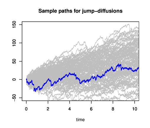
Figure 1: Paths of the jump-diffusion process (3.3) with $(\mu,\sigma,\lambda,m,u)=(20,10,5,3,0)$. We assume that the blue line is an observed process, and the gray liens are other scenarios.

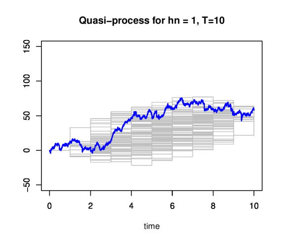
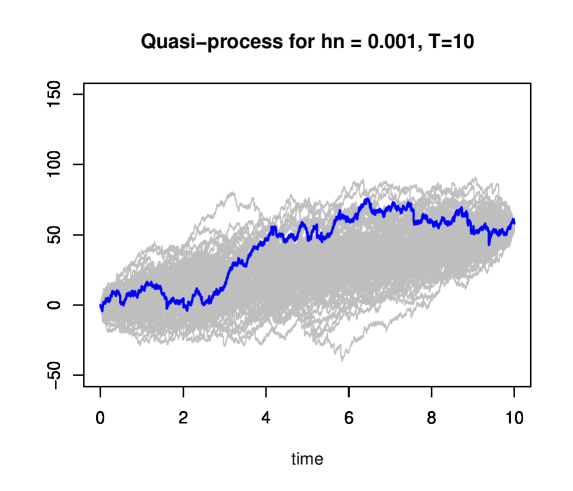
Figure 2: Gray paths are $100(=\alpha_{n})$ quasi-processes based on the discrete samples from the blue observed process with $T=10$. (top: $h_{n}=1.0$; bottom: $h_{n}=0.1$).

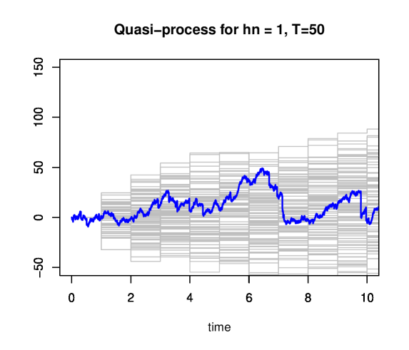
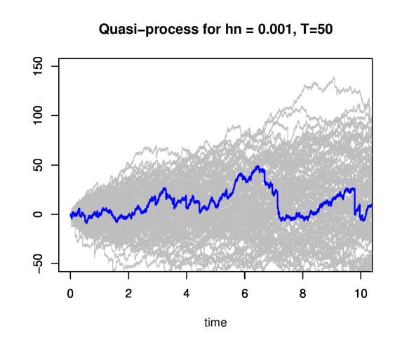
Figure 3: Gray paths are $100(=\alpha_{n})$ quasi-processes based on the discrete samples from the blue observed process with $T=50$. (top $h_{n}=1.0$; bottom: $h_{n}=0.05$).

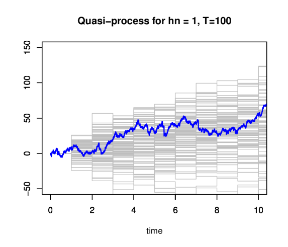
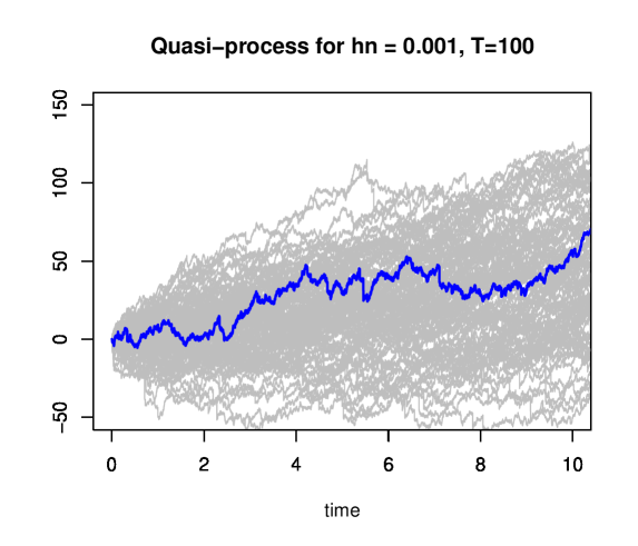
Figure 4: Gray paths are $100(=\alpha_{n})$ quasi-processes based on the discrete samples from the blue observed process with $T=100$. (top: $h_{n}=1.0$; bottom: $h_{n}=0.005$).

Next, let us we compare the marginal distribution of $X_{1}$ and that of the quasi-process, $\widehat{X}_{1}^{i,n}$, under the same parameter values as in the previous experiments. Figures 5 – 7 show histograms of 1000 values of $X_{1}$ from the true distribution and its estimated density (blue solid curve) with $T=10,50$ and $100$. At the same time, estimated densities of $\widehat{X}_{1}^{i,n}$ with $h_{n}=1$ (purple dotted curve), $h_{n}=0.01$ (green dashed curve), and $h_{n}=0.005$ (red solid curve). From those, we can observe the convergence of the marginal distribution when $h_{n}\to 0$ and $T\to\infty$.

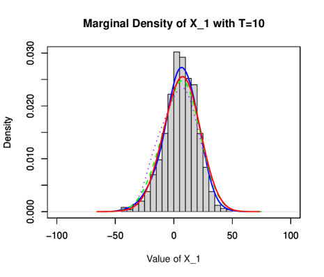
Figure 5: The blue curve is the estimated density of $X_{1}$. The purple dotted curve, the green dashed curve and the red solid curve are estimated densities of quasi-processes when $T=10$ with $h_{n}=1,0.01$ and $0.005$, respectively.

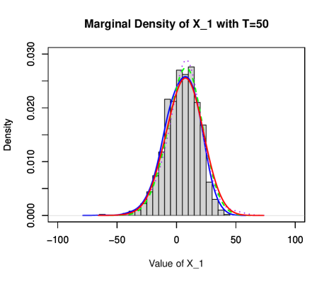
Figure 6: The blue curve is the estimated density of $X_{1}$. The purple dotted curve, the green dashed curve and the red solid curve are estimated densities of quasi-processes when $T=50$ with $h_{n}=1,0.01$ and $0.005$, respectively.

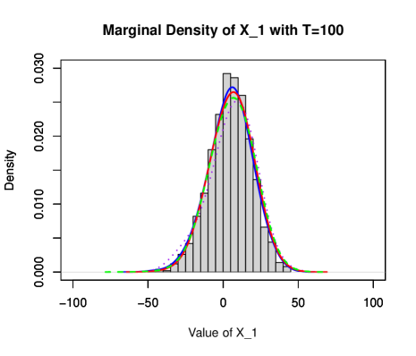
Figure 7: The blue curve is the estimated density of $X_{1}$. The purple dotted curve, the green dashed curve and the red solid curve are estimated densities of quasi-processes when $T=100$ with $h_{n}=1,0.01$ and $0.005$, respectively.

4 Main results for $M$-estimation

4.1 Consistency results

Let $(X^{(\beta)})_{\beta=1,2,\dots,B}$ be independent copies of process $X$ defined on the same probability space $(\Omega,\mathcal{F},{\mathbb{P}})$, and denote its empirical measure as

$${\mathbb{P}}^{*}_{B}=\frac{1}{B}\sum_{\beta=1}^{B}\delta_{X^{(\beta)}}.$$ (4.1)

In the sequel, we assume that, in the empirical measure ${\mathbb{P}}_{\alpha_{n}}$ in (2.1), the permutation samples are taken such that $\alpha_{n}\to\infty$ as $n\to\infty$. Moreover, when ${\cal H}$ is a family of measurable functions $f:\mathbb{D}_{\infty}\times\overline{\Theta}\to\mathbb{R}$, we assume that $\widehat{\vartheta}_{n}$ is given by (2.2) for a given $h_{\vartheta}(x):=h(x,\vartheta)\in{\cal H}$.

Theorem 4.1.

Suppose that $\Theta$ is open bounded subset of $\mathbb{R}^{d}$ with smooth boundary, and that

$${\cal H}\subset C^{0,1}_{b}(\mathbb{D}_{\infty}\times\overline{\Theta}),$$ (4.2)

Moreover, for $h_{\vartheta}(x)\in{\cal H}$, suppose that there exists $\vartheta_{0}\in\Theta$ such that for any ${\epsilon}>0$,

$$\inf_{\vartheta\in\overline{\Theta}:|\vartheta-\vartheta_{0}|>{\epsilon}}Ph_{\vartheta}>Ph_{\vartheta_{0}}.$$ (4.3)

Then $\widehat{\vartheta}_{n}$ is weakly consistent to $\vartheta_{0}$:

$$\widehat{\vartheta}_{n}\stackrel{{\scriptstyle p}}{{\longrightarrow}}\vartheta_{0},\quad n\to\infty.$$

Proof.

It follows for any sequence of permutations $\{i^{n}\}\subset\Lambda_{n}$ that

$$\sup_{\vartheta\in\overline{\Theta}}|({\mathbb{P}}_{\alpha_{n}}-P)h_{\vartheta}| \leq\sup_{\vartheta\in\overline{\Theta}}|({\mathbb{P}}_{\alpha_{n}}-{\mathbb{P}}^{*}_{\alpha_{n}})h_{\vartheta}|+\sup_{\vartheta\in\overline{\Theta}}|({\mathbb{P}}^{*}_{\alpha_{n}}-P)h_{\vartheta}|,$$ (4.4)

and the last second term goes to zero because, under condition (4.2), class ${\cal H}$ is $P$-Glivenko-Cantelli:

$$\sup_{h\in{\cal H}}|({\mathbb{P}}^{*}_{\alpha_{n}}-P)h|=\sup_{\vartheta\in\overline{\Theta}}|({\mathbb{P}}^{*}_{\alpha_{n}}-P)h_{\vartheta}|\to 0\quad a.s.,\quad n\to\infty.$$ (4.5)

To show the convergence of the first term in the last right-hand side of (4.4), we show that

$$\lim_{n\to\infty}\mathbb{E}\left[\sup_{\vartheta\in\overline{\Theta}}\left|\frac{1}{\alpha_{n}}\sum_{k=1}^{\alpha_{n}}\left[h_{\vartheta}(\widehat{X}^{i_{(k)},n})-h_{\vartheta}(X^{(k)})\right]\right|\right]=0,$$ (4.6)

for any sequence of $\{i^{n}\}\subset\Lambda_{n}$.

Note the set $\Theta$ admits a version of Sobolev inequality for embedding $W^{1,p}(\Theta)\hookrightarrow C(\overline{\Theta})$ for $p>d$, that is, for every $f\in W^{1,p}(\Theta)$, it holds that

$$\sup_{\vartheta\in\overline{\Theta}}|f(\vartheta)|^{p}\lesssim\int_{\Theta}\left(|f(\vartheta)|^{p}+|\nabla_{\vartheta}f(\vartheta)|^{p}\right)\,\mathrm{d}\vartheta;$$

see Evans [2], Sec.5.6, Theorem 5. We used this inequality to obtain

$$\mathbb{E}\left[\sup_{\vartheta\in\overline{\Theta}}\left|\frac{1}{\alpha_{n}}\sum_{k=1}^{\alpha_{n}}h_{\vartheta}(\widehat{X}^{i_{(k)},n})-h_{\vartheta}(X^{(k)})\right|^{p}\right]$$ (4.7)

$$\qquad\lesssim\frac{1}{\alpha_{n}}\sum_{k=1}^{\alpha_{n}}\sum_{\ell=0}^{1}\int_{\Theta}\mathbb{E}\left[|\nabla_{\vartheta}^{\ell}h_{\vartheta}(\widehat{X}^{i_{(k)},n})-\nabla_{\vartheta}^{\ell}h_{\vartheta}(X^{(k)})|^{p}\right]\,\mathrm{d}\vartheta$$ (4.8)

$$\qquad=\frac{1}{n!}\sum_{m=1}^{n!}\sum_{\ell=0}^{1}\int_{\Theta}\mathbb{E}\left[|\nabla_{\vartheta}^{\ell}h_{\vartheta}(\widehat{X}^{i_{m},n})-\nabla_{\vartheta}^{\ell}h_{\vartheta}(X)|^{p}\right]\,\mathrm{d}\vartheta,$$ (4.9)

and the last sumands (expectations) go to zero as $n\to\infty$ by Theorem 3.1 and the bounded convergence theorem with the Skorokhood coupling theorem. Hence we have (4.6), and we see that

$$\sup_{\vartheta\in\overline{\Theta}}|({\mathbb{P}}_{\alpha_{n}}-P)h_{\vartheta}|\stackrel{{\scriptstyle p}}{{\longrightarrow}}0,\quad n\to\infty.$$

Together with (4.3), we have the consequence from Theorem 5.7 in van der Vaart [13]. ∎

4.2 Asymptotic normality

For class ${\cal H}$, we denote the bracketing number of ${\cal H}$ by $N_{[\,]}({\epsilon},{\cal H},L^{r}(P))$, which is the minimum number of ${\epsilon}$-brackets, including $[l,u]$, that is a family of measurable functions $f$ satisfying $l\leq f\leq u$ with $\|u-l\|_{L^{r}(P)}<{\epsilon}$, covering ${\cal H}$.

Theorem 4.2.

Considering the same assumptions as in Theorem 4.1, $h_{\vartheta}\in{\cal H}\cap C^{0,2}_{b}(\mathbb{D}_{T}\times\Theta)$ with matrix $V_{\vartheta_{0}}:=P\nabla_{\vartheta}^{2}h_{\vartheta_{0}}$ invertible. Moreover, suppose that there exist a constant $p\,(>d)$ and a sequence $\{r_{n}\}$ with $r_{n}\uparrow\infty$ and $r_{n}^{2}/\alpha_{n}=o(1)$ such that, for $k=0,1$ and any $i^{n}\in\Lambda_{n}$,

$$\left\|\nabla_{\vartheta}^{k}h_{\vartheta}(\widehat{X}^{i^{n},n})-\nabla_{\vartheta}^{k}h_{\vartheta}(X)\right\|_{L^{p}(P)}=o(r_{n}^{-1}),$$ (4.10)

as $n\to\infty$. Then the $M$-estimator $\widehat{\vartheta}_{n}$ is asymptotically normal:

$$\sqrt{r_{n}}(\widehat{\vartheta}_{n}-\vartheta_{0})\leadsto N(0,\Sigma),\quad n\to\infty,$$

with $\Sigma=V_{\vartheta_{0}}^{-1}P[\nabla_{\vartheta}h_{\vartheta_{0}}\nabla_{\vartheta}h_{\vartheta_{0}}^{\top}]V_{\vartheta_{0}}^{-1}$.

Remark 4.1.

Note that $r_{n}$ in Theorem 4.2 is not necessarily unique because, if some $r^{\prime}_{n}$ satisfies (4.10), then $r_{n}=\log r^{\prime}_{n}\uparrow\infty$ also satisfies (4.10). Because we can freely control $\alpha_{n}\,(\leq n!)$, we can attain the $r_{n}$-consistency for various $r_{n}$. If $r_{n}=r_{n}^{*}$ satisfies (4.10) and it holds for $\forall\,\{r^{\prime}_{n}\}$ with $r^{\prime}_{n}/r_{n}^{*}\to\infty$,

$$\liminf_{n\to\infty}r^{\prime}_{n}\|\nabla_{\vartheta}^{k}h_{\vartheta}(\widehat{X}^{i^{n},n})-\nabla_{\vartheta}^{k}h_{\vartheta}(X)\|_{L^{p}}>0,\quad k=0,1.$$

Then this $r_{n}^{*}$ is optimal. In addition, the example in Section 5.1; see Remark 5.1, indicates that several $r_{n}$ can be found and the optimal rate of convergence is attained by choosing $\alpha_{n}$ suitably.

Proof.

We shall use the notation (4.1). Because any function in ${\cal H}$ is Lipschitz with respect to $\vartheta\in\overline{\Theta}$, it follows from, for example, argument as in Example 19.7 in van der Vaart [13], p.271, that the bracketing number of ${\cal H}$ is finite. For every ${\epsilon}>0$,

$$N_{[\,]}({\epsilon},{\cal H},L^{1}(P))\lesssim{\epsilon}^{-d}<\infty,$$

which implies that class ${\cal H}$ is $P$-Donsker, and therefore,

$$\sup_{h\in{\cal H}}|({\mathbb{P}}^{*}_{\alpha_{n}}-P)h|=O_{p}(\alpha_{n}^{-1/2}),\quad n\to\infty.$$

Therefore it follows from the decomposition (4.4) that

$$\sup_{\vartheta\in\overline{\Theta}}|({\mathbb{P}}_{\alpha_{n}}-P)h_{\vartheta}|\leq\sup_{\vartheta\in\overline{\Theta}}|({\mathbb{P}}_{\alpha_{n}}-{\mathbb{P}}^{*}_{\alpha_{n}})h_{\vartheta}|+O_{p}(\alpha_{n}^{-1/2}),$$

Under assumption (4.10), it follows the same argument as in (4.7)-(4.9) that

$$\sup_{\vartheta\in\overline{\Theta}}|({\mathbb{P}}_{\alpha_{n}}-{\mathbb{P}}^{*}_{\alpha_{n}})h_{\vartheta}|=o_{p}(r_{n}^{-1}).$$

Consequently, it holds that

$$\sup_{h\in{\cal H}}|({\mathbb{P}}_{\alpha_{n}}^{*}-{\mathbb{P}}_{\alpha_{n}})h|=O_{p}(\alpha_{n}^{-1/2})+o_{p}(r_{n}^{-1})=o_{p}(r_{n}^{-1}).$$

Considering $|\inf_{n}\alpha_{n}-\inf_{n}b_{n}|\leq\sup_{n}|\alpha_{n}-b_{n}|$ and the definition of $\widehat{\vartheta}_{n}$, we have

$$\left|{\mathbb{P}}_{\alpha_{n}}^{*}h_{\widehat{\vartheta}_{n}}-{\mathbb{P}}_{\alpha_{n}}^{*}h_{\vartheta_{0}}\right| \leq\left|({\mathbb{P}}_{\alpha_{n}}^{*}-{\mathbb{P}}_{\alpha_{n}})h_{\widehat{\vartheta}_{n}}\right|+\left|{\mathbb{P}}_{\alpha_{n}}h_{\widehat{\vartheta}_{n}}-\inf_{\vartheta\in\overline{\Theta}}{\mathbb{P}}_{\alpha_{n}}h_{\vartheta}\right|+\left|\inf_{\vartheta\in\overline{\Theta}}{\mathbb{P}}_{\alpha_{n}}h_{\vartheta}-\inf_{\vartheta\in\overline{\Theta}}{\mathbb{P}}^{*}_{\alpha_{n}}h_{\vartheta}\right|$$

$$\leq 2\sup_{h\in{\cal H}}|({\mathbb{P}}_{\alpha_{n}}^{*}-{\mathbb{P}}_{\alpha_{n}})h|=o_{p}(r_{n}^{-1}),$$

and

$${\mathbb{P}}_{\alpha_{n}}^{*}h_{\widehat{\vartheta}_{n}}\leq{\mathbb{P}}_{\alpha_{n}}^{*}h_{\vartheta_{0}}+o_{p}(r_{n}^{-1})$$

Here, we assume that $h_{\vartheta}\in{\cal H}$ is Lipschitz continuous with respect to $\vartheta\in\overline{\Theta}$. The bracketing number satisfies $N_{[\,]}({\epsilon},{\cal H},L^{2}(P))<\infty$; see Example 19.7 in van der Vaart [13]. Then, using the same argument as in the proof of Corollary 5.53 in van der Vaart [13] with ${\mathbb{P}}_{\alpha_{n}}$ replaced by our ${\mathbb{P}}^{*}_{\alpha_{n}}$, we established that $\sqrt{r_{n}}(\widehat{\vartheta}_{n}-\vartheta_{0})$ is bounded in probability.

Similarly, we have

$$\left|{\mathbb{P}}_{\alpha_{n}}^{*}h_{\widehat{\vartheta}_{n}}-\inf_{\vartheta\in\overline{\Theta}}{\mathbb{P}}_{\alpha_{n}}^{*}h_{\vartheta}\right| \leq\left|{\mathbb{P}}_{\alpha_{n}}^{*}h_{\widehat{\vartheta}_{n}}-\inf_{\vartheta\in\overline{\Theta}}{\mathbb{P}}_{\alpha_{n}}^{*}h_{\vartheta}\right|+\left|\ \inf_{\vartheta\in\overline{\Theta}}{\mathbb{P}}_{\alpha_{n}}^{*}h_{\vartheta}-\inf_{\vartheta\in\overline{\Theta}}{\mathbb{P}}_{\alpha_{n}}^{*}h_{\vartheta}\right|$$

$$\leq\left|{\mathbb{P}}_{\alpha_{n}}^{*}h_{\widehat{\vartheta}_{n}}-{\mathbb{P}}_{\alpha_{n}}h_{\widehat{\vartheta}_{n}}\right|+\sup_{h\in{\cal H}}|({\mathbb{P}}_{\alpha_{n}}^{*}-{\mathbb{P}}_{\alpha_{n}})h|$$

$$\leq 2\sup_{h\in{\cal H}}|({\mathbb{P}}_{\alpha_{n}}^{*}-{\mathbb{P}}_{\alpha_{n}})h|=o_{p}(r_{n}^{-1}),$$

which yields

$${\mathbb{P}}_{\alpha_{n}}^{*}h_{\widehat{\vartheta}_{n}}\leq\inf_{\vartheta\in\overline{\Theta}}{\mathbb{P}}_{\alpha_{n}}^{*}h_{\vartheta}+o_{p}(r_{n}^{-1}).$$ (4.11)

Hence, $\widehat{\vartheta}_{n}$ is approximately a minimum contrast estimator for the contrast function ${\mathbb{P}}^{*}_{\alpha_{n}}h_{\vartheta}$. Hereafter, we can obtain

$$\sqrt{r_{n}}(\widehat{\vartheta}_{n}-\vartheta_{0}) =V_{\vartheta_{0}}^{-1}\frac{1}{\sqrt{\alpha_{n}}}\sum_{i\in A_{n}}\nabla_{\vartheta}h_{\vartheta_{0}}(X^{(i)})+o_{p}(1),\quad n\to\infty.$$

using the same argument as in the proof of Theorem 5.23 in van der Vaart [13] with the condition (4.11): replace ${\mathbb{P}}_{\alpha_{n}}$ with ${\mathbb{P}}_{\alpha_{n}}^{*}$; $n{\mathbb{P}}_{\alpha_{n}}(m_{\vartheta_{0}+\widetilde{h}_{n}/\sqrt{n}}-m_{\vartheta_{0}})$ with $\sqrt{\alpha_{n}r_{n}}{\mathbb{P}}_{\alpha_{n}}^{*}(h_{\vartheta_{0}+\widetilde{h}_{n}/\sqrt{r_{n}}}-h_{\vartheta_{0}})$; $\mathbb{G}_{n}f$ with $\mathbb{G}_{\alpha_{n}}^{*}h_{\vartheta}:=\sqrt{\alpha_{n}}({\mathbb{P}}_{\alpha_{n}}^{*}-P)h_{\vartheta}$ in the proof.

In particular, because $X^{(i)}$’s are IIDs, we conclude by the central limit theorem that

$$\frac{1}{\sqrt{\alpha_{n}}}\sum_{i\in A_{n}}\nabla_{\vartheta}h_{\vartheta_{0}}(X^{(i)})\leadsto N(0,P[\nabla_{\vartheta}h_{\vartheta_{0}}\nabla_{\vartheta}h_{\vartheta_{0}}^{\top}]),\quad\alpha_{n}\to\infty.$$

∎

5 Examples

5.1 Default-related discounted losses

Here, we consider concrete examples for $h_{\vartheta}$ and investigate sufficient conditions that ensure the conditions in Theorems 4.1 and 4.2.

Suppose the Lévy process $X=(X_{t})_{t\in[0,T]}$ with (1.1) represents a ‘loss’ process of a company, and we define the time of default as

$$\tau^{X}:=\inf\{t\in[0,T]\,|\,X_{t}<\xi\}\wedge T,$$

for constants $\xi\in\mathbb{R}$ and $T\in(0,\infty]$. $\tau^{X}$ is interpreted as the time of default (resp. ruin) with default levels $\xi$ in the context of finance (resp. insurance). In this section, we consider a discounted loss up to default. For $x=(x_{t})_{t\in[0,T]}\in\mathbb{D}_{T}$,

$$h_{\vartheta}(x)=h(x,\vartheta)=\int_{0}^{\tau^{x}}e^{-rt}U_{\vartheta}(t,x_{t})\,\mathrm{d}t,.$$ (5.1)

where $r>0$ and $U_{\vartheta}:\mathbb{R}_{+}\times\mathbb{R}\to\mathbb{R}$ are a bounded function with parameter $\vartheta\in\overline{\Theta}\subset\mathbb{R}^{d}$ to be controlled. Then, $Ph_{\vartheta}$ is the expected discounted loss up to default

$$Ph_{\vartheta}=\mathbb{E}\left[\int_{0}^{\tau^{X}}e^{-rt}U_{\vartheta}(t,X_{t})\,\mathrm{d}t\right];$$ (5.2)

see Feng and Shimizu [4] for details on this quantity.

In the sequel, we consider the Skorokhod space $(\mathbb{D}_{T},\varrho_{T})$, where $\varrho_{T}$ is the Skorokhod metric given in Section 1.

Lemma 5.1.

Let $T\in(0,\infty]$. The functional $\tau^{\cdot}$ defined on $\mathbb{D}_{T}$ is continuous with respect to $\varrho_{T}$; that is, for any $x,y\in\mathbb{D}_{T}$ and ${\epsilon}>0$, there exists a $\delta>0$ such that

$$\varrho_{T}(x,y)<\delta\quad\Rightarrow\quad|\tau^{x}-\tau^{y}|<{\epsilon}.$$

Proof.

Note that the functional

$$F(x;T_{1},T_{2})=\inf_{T_{1}\leq s\leq T_{2}}x_{s},\quad 0\leq T_{1}<T_{2}\leq T,$$

in $x\in\mathbb{D}_{T}$ is continuous in the sense of the Skorokhod metric $\varrho_{T}$, and it follows for each $y\in\mathbb{D}_{T}$ and $\eta>0$, there exists a constant $\delta:=\delta(y,\eta)>0$ such that when $\varrho_{T}(x,y)<\delta$,

$$\left|F(x;\tau^{y}-{\epsilon},\tau^{y}+{\epsilon})-F(y;\tau^{y}-{\epsilon},\tau^{y}+{\epsilon})\right|<\eta,$$

which implies that

$$\inf_{\tau^{y}-{\epsilon}\leq s\leq\tau^{y}+{\epsilon}}x_{s}<\inf_{\tau^{y}-{\epsilon}\leq s\leq\tau^{y}+{\epsilon}}y_{s}+\eta.$$

Because $\inf_{\tau^{y}-{\epsilon}\leq s\leq\tau^{y}+{\epsilon}}y_{s}<\xi$ by the definition of $\tau^{y}$, when $\eta>0$ is sufficiently small, we have

$$\inf_{\tau^{y}-{\epsilon}\leq s\leq\tau^{y}+{\epsilon}}x_{s}<\xi,$$

which is equivalent to $|\tau^{x}-\tau^{y}|<{\epsilon}$. ∎

Lemma 5.2.

Let $N\geq 2$ be an integer and $T\in(0,\infty]$. For bounded function $U_{\vartheta}:\mathbb{R}_{+}\times\mathbb{R}\to\mathbb{R}$ with parameter $\vartheta\in\Theta\subset\mathbb{R}^{d}$, suppose that the derivatives up to $N$th order with respect to $\vartheta$ are uniformly bounded

$$\sup_{(t,z)\in\mathbb{R}_{+}\times\mathbb{R};\vartheta\in\overline{\Theta}}|\nabla_{\vartheta}^{k}U_{\vartheta}(t,z)|\leq C,\quad k=0,1,\dots,N,$$ (5.3)

for constant $C>0$. Moreover, suppose the Lipschitz continuity:

$$\sup_{t\in\mathbb{R}_{+};\vartheta\in\overline{\Theta}}|\nabla_{\vartheta}^{k}U_{\vartheta}(t,x)-\nabla_{\vartheta}^{k}U_{\vartheta}(t,y)|\leq L\|x-y\|_{T},\quad x,y\in\mathbb{D}_{T},\ k=1,\dots,N.$$ (5.4)

Then the functional (5.1) satisfies that

$$h\in C_{b}^{0,k}(\mathbb{D}_{T}\times\Theta),\quad k=1,\dots,N-1.$$

Proof.

In this proof, we arbitrarily fix $\vartheta\in\overline{\Theta}$ and simply write $h(x):=h(x,\vartheta)$.

For any $x,y\in\mathbb{D}_{T}$ and any increasing surjection $\lambda:[0,T]\to[0,T]$

$$|h(x)-h(y)| =\left|\int_{0}^{\tau^{x}}e^{-rt}U_{\vartheta}(t,x_{t})\,\mathrm{d}t-\int_{0}^{\tau^{y}}e^{-rt}U_{\vartheta}(t,y_{t})\,\mathrm{d}t\right|\left(\mathbf{1}_{\{\tau^{x}\geq\tau^{y}\}}+\mathbf{1}_{\{\tau^{x}<\tau^{y}\}}\right)$$

$$=\left|\int_{\tau^{y}}^{\tau^{x}}e^{-rt}U_{\vartheta}(t,x_{t})\,\mathrm{d}t+\int_{0}^{\tau^{y}}e^{-rt}\left[U_{\vartheta}(t,x_{t})-U_{\vartheta}(t,y_{t})\right]\,\mathrm{d}t\right|\mathbf{1}_{\{\tau^{x}\geq\tau^{y}\}}$$

$$\quad+\left|\int_{\tau^{x}}^{\tau^{y}}e^{-rt}U_{\vartheta}(t,y_{t})\,\mathrm{d}t+\int_{0}^{\tau^{x}}e^{-rt}\left[U_{\vartheta}(t,y_{t})-U_{\vartheta}(t,x_{t})\right]\,\mathrm{d}t\right|\mathbf{1}_{\{\tau^{x}<\tau^{y}\}}$$

$$\leq C|\tau^{x}-\tau^{y}|+\int_{0}^{T}e^{-rt}|U_{\vartheta}(t,x_{t})-U_{\vartheta}(t,y_{t})|\,dt$$

$$=C|\tau^{x}-\tau^{y}|+\int_{0}^{T}e^{-r\lambda(t)}|U_{\vartheta}(\lambda(t),x\circ\lambda(t))-U_{\vartheta}(\lambda(t),y\circ\lambda(t))|\lambda^{\prime}(t)\,dt$$

$$\leq C|\tau^{x}-\tau^{y}|+\int_{0}^{T}e^{-r\lambda(t)}|U_{\vartheta}(\lambda(t),x\circ\lambda(t))-U_{\vartheta}(\lambda(t),y_{t})|\lambda^{\prime}(t)\,dt$$

$$\quad+\int_{0}^{T}e^{-r\lambda(t)}|U_{\vartheta}(\lambda(t),y\circ\lambda(t))-U_{\vartheta}(\lambda(t),y_{t})|\lambda^{\prime}(t)\,dt$$

$$\leq C|\tau^{x}-\tau^{y}|+L\max\{\|x\circ\lambda-y\|_{T},\|\lambda-I\|_{T}\}\int_{0}^{T}\lambda^{\prime}(t)e^{-r\lambda(t)}\,dt$$

$$\quad+L\max\{\|y\circ\lambda-y\|_{T},\|\lambda-I\|_{T}\}\int_{0}^{T}\lambda^{\prime}(t)e^{-r\lambda(t)}\,dt$$

$$\leq C|\tau^{x}-\tau^{y}|+r^{-1}L\max\{\|x\circ\lambda-y\|_{T},\|\lambda-I\|_{T}\}$$

$$\quad+r^{-1}L\max\{\|y\circ\lambda-y\|_{T},\|\lambda-I\|_{T}\},$$

where $I$ is the identity map of $[0,T]$. In the last inequality, we use that $U_{\vartheta}$ is Lipschitz continuous with the Lipschitz constant $L>0$. Consider the infimum with respect to $\lambda\in\Lambda_{T}$ on both sides to obtain

$$|h(x)-h(y)|\lesssim|\tau^{x}-\tau^{y}|+\varrho_{T}(x,y).$$

This inequality with Lemma 5.1 implies that $h$ is continuous on $(\mathbb{D}_{T},\varrho_{T})$.

Because $\nabla_{\vartheta}^{k}h(x,\vartheta)=\int_{0}^{\tau^{x}}e^{-rt}\nabla_{\vartheta}^{k}U_{\vartheta}(t,x_{t})\,\mathrm{d}t\ (k\leq N)$ under this assumption, the same argument is valid for $\nabla_{\vartheta}^{k}h(\cdot,\vartheta)\ (k\leq N-1)$. ∎

Lemma 5.3.

Suppose we use the same assumptions as in Lemma 5.2, and that there exist constants $p>d=\dim(\Theta)$ and $q>0$ as well as sequence $\{\gamma_{n}\}$ with $\gamma_{n}\uparrow\infty$ such that

$$\sup_{i\in A_{n}}\|\widehat{X}_{t}^{i,n}-X_{t}\|_{L^{p}}\leq t^{q}\cdot o(\gamma_{n}^{-1}),\quad n\to\infty.$$ (5.5)

For each $t>0$, where $o(\gamma_{n}^{-1})$-term is independent of $t$. Then it follows for each $i^{n}\in A_{n}$ and any $p>d$ that

$$\left\|\nabla_{\vartheta}^{k}h_{\vartheta}(\widehat{X}^{i^{n},n})-\nabla_{\vartheta}^{k}h_{\vartheta}(X)\right\|_{L^{p}}=o(\gamma_{n}^{-1}),\quad k\leq N-1$$

Proof.

For any integer $k\leq N-1$, $\nabla_{\vartheta}^{k}U_{\vartheta}$ is the Lipschitz continuous with respect to $\vartheta$ uniformly in $x$ under the assumptions in Lemma 5.2. Hence, it follows for any $p\geq 1$ that

$$\Big{\|}\nabla_{\vartheta}^{k}h_{\vartheta}(\widehat{X}^{i^{n},n})-\nabla_{\vartheta}^{k}h_{\vartheta}(X)\Big{\|}_{L^{p}} \leq\int_{0}^{\infty}e^{-rt}\left\|\nabla_{\vartheta}^{k}U(t,\widehat{X}_{t}^{i^{n},n})-\nabla_{\vartheta}^{k}U(t,X_{t})\right\|_{L^{p}}\,\mathrm{d}t$$

$$\lesssim\int_{0}^{\infty}e^{-rt}\|\widehat{X}_{t}^{i^{n},n}-X_{t}\|_{L^{p}}\,\mathrm{d}t$$

$$\leq o(\gamma_{n}^{-1})\int_{0}^{\infty}t^{q}e^{-rt}\,\mathrm{d}t,$$

which implies (4.10) in Theorem 4.2. ∎

We can check the condition (5.5) by taking the sampling interval $h_{n}$ suitably, as in the following Lemma:

Lemma 5.4.

Suppose that $h_{n}=n^{-\beta}$ for some $\beta\in(0,1)$. Hereafter, the condition (5.5) holds with $\gamma_{n}=n^{\beta/p}$ for any $p>d$.

Proof.

Recall that

$$\widehat{X}_{t_{k}}^{i^{n},n}=\mu+\sum_{l=1}^{k-1}\Delta_{i^{n}(l)}X,\quad X_{t_{k}}=\mu+\sum_{l=1}^{k-1}\Delta_{l}X,\quad t_{k}=kh_{n}$$

Hereafter, it follows that

$$\hat{X}_{t_{k}}^{i^{n},n}-X_{t_{k}} =\sum_{l=1}^{k-1}\Delta_{i^{n}(l)}X-\sum_{l=1}^{k-1}\Delta_{l}X=\sum_{c=0}^{k-1}\sum_{i^{n}\in B_{n,k,c}}(\Delta_{i^{n}(l)}-\Delta_{l^{\prime}}X)$$

$$=^{d}\sum_{c=0}^{k-1}\sum_{i\in B_{n,k,c}}(k-c)\bm{1}_{\{i^{n}=i\}}(\Delta_{1}X-\Delta_{2}X),$$

where $B_{n,k,c}=\{i\in\Lambda_{n}|\#\{\{i(1),\ldots,i(k)\}\cap\{1,\ldots,k\}\}=c\}$, which is the number of pairs $(i^{n}(l),l^{\prime})$with $i^{n}(l)=l^{\prime}$ in $l,l^{\prime}\in\{1,\ldots,k\}$ is equal to $c$. Here, we claim that the number of $i\in\Lambda_{n}$ such that $\#\{\{i(1),\ldots,i(k)\}\cap\{1,\ldots,k\}\}=c$ is

$${k\choose c}\cdot{{n-k}\choose{k-c}}\cdot k!(n-k)!.$$

Generally, it follows from the Vandermonde’s formula $\sum_{j=0}^{k}{n\choose j}{m\choose k-j}={n+m\choose k}$ that

$$\sum_{c=0}^{k}{k\choose c}{n-k\choose k-c}k!(n-k)!={n\choose k}\frac{k!(n-k)!}{n!}n!=\#\Lambda_{n},$$

for each $k$. Therefore, we have

$$\sum_{c=0}^{k-1} {k\choose c}{n-k\choose k-c}k!(n-k)!\times(k-c)=\frac{(n-1)!}{(k-1)!(n-k-1)!}k!(n-k)!\leq n!k$$

and that

$$\|\hat{X}_{t_{k}}^{i^{n},n}-X_{t_{k}}\|_{L^{p}} =\left\|\sum_{c=0}^{k-1}\sum_{i\in B_{n,k,c}}(k-c)\bm{1}_{\{i^{n}=i\}}(\Delta_{1}X-\Delta_{2}X)\right\|_{L^{p}}$$

$$\leq\sum_{c=0}^{k-1}\sum_{i\in B_{n,k,c}}(k-c)\mathbb{P}\left(i^{n}=i\right)\left\|(\Delta_{1}X-\Delta_{2}X)\right\|_{L^{p}}$$

$$\leq n!\times k\mathbb{P}(i^{n}=i)\left\|(\Delta_{1}X-\Delta_{2}X)\right\|_{L^{p}}$$

$$=n!\times k\times\frac{1}{n!}\left\|(\Delta_{1}X-\Delta_{2}X)\right\|_{L^{p}}$$

$$\lesssim k\cdot O(r_{n}^{-1}).$$

Taking $h_{n}=n^{-\beta}$ ($0<\beta<1$) and $q>2$, we observe that

$$\frac{\|\hat{X}_{t_{k}}^{i^{n},n}-X_{t_{k}}\|_{L^{p}}}{(t_{k})^{q}}\lesssim\frac{k}{(kh_{n})^{q}}O(r_{n}^{-1})=k^{1-q}\cdot n^{q\beta}O(r_{n}^{-1})\leq n^{1-q+q\beta}O(r_{n}^{-1})$$

Hence, when we take $q>1/(1-\beta)$, it holds that

$$\|\hat{X}_{t_{k}}^{i^{n},n}-X_{t_{k}}\|_{L^{p}}=(t_{k})^{q}\cdot o(r_{n}^{-1}).$$

∎

Remark 5.1.

Note that the rate $\gamma_{n}$ in the above proof depends on $p>d$, which means that, by Theorem 4.2, we can obtain the rate of convergence $\sqrt{n^{\beta/p}}$ for each $p>d$:

$$\sqrt{n^{\beta/p}}(\widehat{\vartheta}_{n}-\vartheta_{0})\leadsto N(0,\Sigma),\quad n\to\infty,$$

by controlling the resampling number $\alpha_{n}$ such that $\alpha_{n}/n^{\beta/p}=o(1)$, where $\Sigma$ is given in Theorem 4.2. Hereafter, we can access the optimal rate $\sqrt{n^{\beta/d}}$ by letting $p\downarrow d$.

5.2 Dividends up to ruin

In the dividends problem, we can consider a case where $U_{\vartheta}$ in (5.2) is of the form

$$U_{\vartheta}(x,t)=\alpha\mathbf{1}_{\{x\geq\vartheta\}}\mathbf{1}_{\{t\leq g(\vartheta)\}},$$

where $\alpha>0$ is a constant and $g$ is an increasing function in $\vartheta\in\overline{\Theta}$. Assuming that a surplus of an insurance company $x=(x_{t})_{t\geq 0}$ is given, the functional

$$h_{\vartheta}(x)=\int_{0}^{\tau^{x}}e^{-rt}U_{\vartheta}(t,x_{t})\,\mathrm{d}t$$

is interpreted as the aggregate dividends paid up to ruin $x_{t}<\xi$ or maturity $g(\vartheta)$ depending on the parameter $\vartheta$, where the dividend $\alpha$ is paid when the surplus $x_{t}$ is over the threshold $\vartheta$, and the maturity depends on the threshold. That is, when the threshold level is high (the dividends are hard to pay), the maturity for dividends will be longer, but the maturity will be shorter when the threshold level is low (the dividends are easy to pay). Because the ruin level is $\xi>0$, the threshold $\vartheta$ should be set over $\xi$, and we assume that $\Theta=[\xi,M]$ for constant $M>0$.

For technical reasons, we replace the indicator function $\mathbf{1}_{\{u\geq z\}}$ with $\varphi_{\epsilon}(u,z)\in C^{\infty}(\mathbb{R}\times\mathbb{R})$ with bounded derivatives such that

$$\varphi_{\epsilon}(u,z)=\left\{\begin{array}[]{cc}1&(u\geq z+{\epsilon})\\ 0&(u\leq z-{\epsilon})\end{array}\right.$$

for a ‘small’ constant ${\epsilon}>0$. That is, we can replace the following indicators as:

$$\mathbf{1}_{\{x_{t}\geq\vartheta\}}\quad \Rightarrow\quad\varphi_{\epsilon}(x_{t},\vartheta)$$

$$\mathbf{1}_{\{t\leq g(\vartheta)\}}\quad \Rightarrow\quad\varphi_{\epsilon}(\vartheta,g^{-1}(t))$$

Hereafter, the functional $h$ can be approximated by

$$h_{\vartheta}^{\epsilon}(x)=\alpha\int_{0}^{\tau^{x}}e^{-rt}\varphi_{\epsilon}(x_{t},\vartheta)\varphi_{\epsilon}(\vartheta,g^{-1}(t))\,\mathrm{d}t$$

This approximation is valid because it follows by the bounded convergence theorem that

$$\lim_{{\epsilon}\to 0}h_{\vartheta}^{\epsilon}(X)=\alpha\int_{0}^{\tau^{x}}e^{-rt}\lim_{{\epsilon}\to 0}\left[\varphi_{\epsilon}(x_{t},\vartheta)\varphi_{\epsilon}(\vartheta,g^{-1}(t))\right]\,\mathrm{d}t=h_{\vartheta}(x),\quad x\in\mathbb{D}_{T}.$$

Moreover, because the derivatives of $\varphi_{\epsilon}$ are uniformly bounded, it follows that for fixed ${\epsilon}>0$ and $k\in\mathbb{N}$,

$$\nabla_{\vartheta}^{k}U_{\vartheta}^{\epsilon}(x,t)=\alpha\nabla_{\vartheta}^{k}\left[\varphi_{\epsilon}(x_{t},\vartheta)\varphi_{\epsilon}(\vartheta,g^{-1}(t))\right]$$

satisfies conditions (5.3) and (5.4) in Lemma 5.2. Hereafter, Theorem 4.2 is applicable for $h^{\epsilon}_{\vartheta}(X)$ with the Lévy process $X=(X_{t})_{t\geq 0}$. Further examples will be discussed in a different paper; Shimizu and Shiraishi [12].

Acknowledgments

The first author was partially supported by JSPS KAKENHI Grant Numbers JP21K03358 and JST CREST JPMJCR14D7, Japan. The second author was supported by JSPS KAKENHI Grant Number JP16K00036.

References

- [1] Billingsley, P. (1999). Convergence of probability measures. 2nd ed. John Wiley & Sons, New York.
- [2] Evans, L. C. (2010). Partial differential equations, 2nd ed., American Mathematical Society, Providence, RI.
- [3] Feng, R. (2011). An operator-based approach to the analysis of ruin-related quantities in jump diffusion risk models. Insurance: Mathematics and Economics, 48 (2), 304–313.
- [4] Feng, R. and Shimizu, Y. (2013). On a generalization from ruin to default in a Lévy insurance risk model. Methodol. Comput. Appl. Probab., 15, (4), 773–802.
- [5] Comte, F. and Genon-Catalot, V. (2011). Estimation for Lévy processes from high frequency data within a long term interval. The Annals of Statistics, 39, (2), 803–837.
- [6] Gerber, H. U. and Shiu, E. S. W. (1997). From ruin theory to pricing reset guarantees and perpetual put options, Insurance: Math. and Econom., 24, 3–14.
- [7] Jacod, J. (2007). Asymptotic properties of power variations of Lévy processes. ESAIM Probab. Statist. 11, 173–196.
- [8] Kato, K. and Kurisu, D. (2020). Bootstrap confidence bands for spectral estimation of L évy densities under high-frequency observations. Stoch. Proc. Appl., 130, (3), 1159–1205.
- [9] Kuratowski, K. (1966). Topology I. Academic Press, New York.
- [10] Mammen, E. (1992). When Does Bootstrap Work?: Asymptotic Results and Simulations, Springer-Verlag, New York.
- [11] Shimizu, Y. (2009). Functional estimation for Lévy measures of semimartingales with Poissonian jumps. J. Multivariate Anal., 100, (6), 1073–1092.
- [12] Shimizu, Y. and Shiraishi, H. (2022). Semiparametric Estimation of Optimal Dividend Barrier for Spectrally Negative Lévy Process, preprint.
- [13] van der Vaart, A. W. (1998). Asymptotic Statistics. Cambridge University Press, Cambridge.
- [14] van der Vaart, A. W. and Wellner, J. A. (1996). Weak Convergence and Empirical Processes: With Applications to Statistics. Springer, New York.