ALMA-IMF I - Investigating the origin of stellar masses: Introduction to the Large Program and first results

Abstract

Aims. Thanks to the high angular resolution, sensitivity, image fidelity, and frequency coverage of ALMA, we aim to improve our understanding of star formation. One of the breakthroughs expected from ALMA, which is the basis of our Cycle 5 ALMA-IMF Large Program, is the question of the origin of the initial mass function (IMF) of stars. Here we present the ALMA-IMF protocluster selection, first results, and scientific prospects.

Methods. ALMA-IMF imaged a total noncontiguous area of $\sim$53 pc², covering extreme, nearby protoclusters of the Milky Way. We observed 15 massive ($2.5-33\times 10^{3}\leavevmode\nobreak\ \mbox{$M_{\odot}$}$), nearby ($2-5.5$ kpc) protoclusters that were selected to span relevant early protocluster evolutionary stages. Our 1.3 mm and 3 mm observations provide continuum images that are homogeneously sensitive to point-like cores with masses of $\sim$0.2 $M_{\odot}$ and $\sim$0.6 $M_{\odot}$, respectively, with a matched spatial resolution of $\sim$2 000 au across the sample at both wavelengths. Moreover, with the broad spectral coverage provided by ALMA, we detect lines that probe the ionized and molecular gas, as well as complex molecules. Taken together, these data probe the protocluster structure, kinematics, chemistry, and feedback over scales from clouds to filaments to cores.

Results. We classify ALMA-IMF protoclusters as Young (six protoclusters), Intermediate (five protoclusters), or Evolved (four protoclusters) based on the amount of dense gas in the cloud that has potentially been impacted by H ii region(s). The ALMA-IMF catalog contains $\sim$700 cores that span a mass range of $\sim$0.15 $M_{\odot}$ to $\sim$250 $M_{\odot}$ at a typical size of $\sim$2 100 au. We show that this core sample has no significant distance bias and can be used to build core mass functions (CMFs) at similar physical scales. Significant gas motions, which we highlight here in the G353.41 region, are traced down to core scales and can be used to look for inflowing gas streamers and to quantify the impact of the possible associated core mass growth on the shape of the CMF with time. Our first analysis does not reveal any significant evolution of the matter concentration from clouds to cores (i.e., from 1 pc to 0.01 pc scales) or from the youngest to more evolved protoclusters, indicating that cloud dynamical evolution and stellar feedback have for the moment only had a slight effect on the structure of high-density gas in our sample. Furthermore, the first-look analysis of the line richness toward bright cores indicates that the survey encompasses several tens of hot cores, of which we highlight the most massive in the G351.77 cloud. Their homogeneous characterization can be used to constrain the emerging molecular complexity in protostars of high to intermediate masses.

Conclusions. The ALMA-IMF Large Program is uniquely designed to transform our understanding of the IMF origin, taking the effects of cloud characteristics and evolution into account. It will provide the community with an unprecedented database with a high legacy value for protocluster clouds, filaments, cores, hot cores, outflows, inflows, and stellar clusters studies.

1 Introduction

The relative number of stars born with masses between $0.01\leavevmode\nobreak\ \mbox{$M_{\odot}$}$ and $>$100 $M_{\odot}$, the so-called initial mass function (IMF), is among the very few key parameters transcending astrophysical fields. For example, it is critically important for cosmology and stellar physics (Madau & Dickinson 2014; Hopkins 2018). In studies of both the Galactic and cosmic history of star formation, the IMF is often considered to be universal (e.g., Bastian et al. 2010; Kroupa et al. 2013). A few studies of young massive stellar clusters in the Milky Way (Lu et al. 2013; Maia et al. 2016; Hosek et al. 2019) or in nearby galaxies (Schneider et al. 2018) and indirect constraints at high redshift (Smith 2014; Zhang et al. 2018) suggest, however, incidences of IMFs with noncanonical, top-heavy shapes (see the recent review by Hopkins 2018). The IMF also varies with metallicity, becoming top-heavy or bottom-heavy in low- or high-metallicity environments, respectively (e.g., Marks et al. 2012; Martín-Navarro et al. 2015). Overall, the IMF may not be as universal as once thought, but may vary with galactic environment and evolve over time. Therefore, the central astrophysical importance of the IMF motivates a vigorous investigation into the question of its origin.

In the star-formation community, both the IMF origin and its dependence on environment remain the subject of heated debate (see reviews by Offner et al. 2014; Krumholz 2015; Ballesteros-Paredes et al. 2020; Lee et al. 2020). In the star-forming regions studied in the last two decades, the mass distribution of cores, the core mass function (CMF), is strikingly similar to the IMF (e.g., Motte et al. 1998, 2001; Testi & Sargent 1998; Alves et al. 2007; Enoch et al. 2008; Könyves et al. 2015). These studies, which were conducted in Gould Belt clouds, star-forming regions in the solar neighborhood that form solar-type stars, led to the interpretation that the shape of the IMF may simply be inherited from the CMF. These nearby regions are, however, unrepresentative of the larger Milky Way. For instance, they do not capture clouds that form stars more massive than $5\leavevmode\nobreak\ \mbox{$M_{\odot}$}$, high-mass cloud environments, or the vast extent and range of conditions in the Galaxy. Our current understanding of the origin of stellar masses is therefore biased. Massive protoclusters are key laboratories for the study of the emergence of the IMF because these clusters of cores are the gas-dominated cradles of rich star clusters, probing substantially different, and cosmically important, environments. A detailed scrutiny and study of statistical samples of massive protoclusters is mandatory to test observationally whether the IMF origin is in fact independent of cloud characteristics or not. The ALMA-IMF Large Program (PIs: Motte, Ginsburg, Louvet, Sanhueza) is a survey of 15 nearby Galactic protoclusters observed at matched sensitivity and physical resolution that aims for statistically meaningful results on the origin of the IMF (see below).

Even before studying the relationship between the IMF and the CMF, it is important to realize that how the IMF originates from the observed CMF depends directly on the definition of the cores, assumed to be the gas mass reservoir used for the formation of each star or binary system. As shown by Louvet et al. (2021), defining this mass reservoir may seem obvious in the observed map of a cloud, but core characteristics (size, mass) depend heavily on the spatial scales probed by the observations. In addition, the theoretical definition of cores also depends on whether the star-formation scenario is quasi-static or dynamic. In the former scenario, cores are gas condensations sufficiently dense to be on the verge of gravitational collapse, and they convert the core gas into stars (Shu et al. 1987; Chabrier 2003; McKee & Ostriker 2007; André et al. 2014). After a quasi-static phase of concentration of the cloud gas into cores, cores become distinct from their surrounding cloud and start to collapse, and their future stellar content becomes independent of the properties of the parental cloud. In the latter scenario, dynamics play a major role during all phases of the star-formation process (e.g., Ballesteros-Paredes et al. 2007; Hennebelle & Falgarone 2012; Padoan et al. 2014). In particular, global infall of filament networks and gas inflow toward cores are expected to be important drivers of star formation (e.g., Smith et al. 2009; Vázquez-Semadeni et al. 2019; Padoan et al. 2020). In this framework, filaments, cores, and stellar embryos simultaneously accrete gas, and the gas reservoir associated with star formation largely exceeds the extent of the observed cores. This so-called clump-fed scenario was proposed in various recent papers and described in detail in the review by Motte et al. (2018a, see references therein). One of the main objectives of the ALMA-IMF Large Program is to discriminate between the quasi-static and dynamic scenarios by quantifying the role of cloud kinematics in defining core mass and in possibly changing it over time.

In the ALMA-IMF pilot study, Motte et al. (2018b) identified the first definitive observation of a CMF whose shape differs from that of the IMF. The authors derived this CMF in W43-MM1, which is a dense cloud efficiently forming stars at the tip of the Galactic bar (Nguyen-Luong et al. 2013; Louvet et al. 2014). Fitted by a single power-law relation in both the solar-type and high-mass regimes ($2-100\leavevmode\nobreak\ \mbox{$M_{\odot}$}$ cores, thus $\sim$1$-50\leavevmode\nobreak\ \mbox{$M_{\odot}$}$ stars with a $50\%$ conversion efficiency; Motte et al. 2018b), this CMF is flatter than those of reference CMF studies from nearby, low-mass star-forming regions (e.g., Motte et al. 1998; Könyves et al. 2015; Di Francesco et al. 2020). It is also quantitatively flatter than the CMF derived from a one-to-one mapping of the high-mass end, $m\geq 1\leavevmode\nobreak\ \mbox{$M_{\odot}$}$, of the stellar IMF, ${\rm d}N/{\rm d}\log(m)\propto m^{-1.35}$ (Salpeter 1955; Kroupa 2001). Such an excess of high-mass cores with respect to their solar-type counterparts indicates a top-heavy CMF. This was previously suggested by single-pointing observations (e.g., Bontemps et al. 2010; Zhang et al. 2015) but could not be substantiated further than a mass segregation effect. Top-heavy CMFs were also observed in combined CMFs, built from the combination of cores extracted in a dozen to several dozen massive clumps (Csengeri et al. 2017; Liu et al. 2018; Sanhueza et al. 2019; Sadaghiani et al. 2020; Lu et al. 2020; O’Neill et al. 2021). To date, the only two statistically significant studies carried out on single massive clouds are those of Motte et al. (2018b) and Kong (2019). If confirmed, these results challenge either the direct relation between the CMF and the IMF or the IMF universality, and most probably both.

To achieve the objectives of ALMA-IMF, we must tackle both individual cores and their connection to the larger-scale cloud environment, which is most immediately accessible via kinematics. Following the nomenclature in Motte et al. (2018a), but adapting the definitions to gas structures containing massive protoclusters, clouds are a few parsecs in size, clumps are structures on intermediate scales on the order of a few times $\sim$0.1 pc, and cores are $\sim$0.01 pc in size. Cores could subfragment, making them the precursors of either single star or multiples stars, but they will not form stellar clusters. The large spectral coverage of ALMA makes it possible to simultaneously image molecular lines that characterize both cores and clouds. The presence of outflows and infall, often traced by CO, SiO, CS, and HCO⁺ lines, typically provides the first indication of the evolutionary nature of the cores that can be pre-stellar or protostellar. In addition, as the luminosity of the protostars increases, they further interact with their immediate surroundings, creating hot cores and, for the most massive, H ii regions. Hot cores classically correspond to high-mass protostellar objects (e.g., Kurtz et al. 2000; Cesaroni 2005), which are dominated by radiatively heated gas above 100 K. At these temperatures, the ice mantles of the dust grains formed in the cold, high-density medium of cores evaporate (e.g. Herbst & van Dishoeck 2009). Hot cores are therefore associated with a rich molecular content observed by a large number of lines from complex organic molecules (COMs; e.g., Gibb et al. 2000; Schilke et al. 2006). Considering the formation of dense cloud structures (filaments and cores $>$10⁵ cm^-3), the most abundant, light molecules (such as CO, N₂H⁺, and CS) are typically used to probe the gas density and kinematics. The kinematics of dominant filaments in low- and high-mass star-forming regions have already been studied in some detail (e.g., Schneider et al. 2010; Peretto et al. 2013; Fernández-López et al. 2014; Battersby et al. 2014; Stutz 2018; Hacar et al. 2018; Jackson et al. 2019); however, very little is known about the gas feeding of cores (Galván-Madrid et al. 2009; Csengeri et al. 2011b; Olguin et al. 2021; Sanhueza et al. 2021). This process must now be a priority for CMF studies because constraints on any hierarchical inflow of gas could link cloud kinematics to the growth of core mass.

To deepen our understanding of the IMF origin and quantify the CMF dependence, if any, with respect to the properties of clouds over their lifetimes, various cloud environments must be sampled. Observational limitations lead to initiating such work by targeting the most massive and closest protoclusters in our Milky Way, as was done by, for example, Motte et al. (2018b) and Sanhueza et al. (2019). During the past decade, the APEX/ATLASGAL, CSO/BGPS, and Herschel/HiGAL surveys have covered the inner Galactic plane at (sub)millimeter and far-infrared wavelengths, providing complete samples of $0.1-1$ pc clumps up to distances of at least 8 kpc (Ginsburg et al. 2013; Csengeri et al. 2014; König et al. 2017; Elia et al. 2021). From the CSO/BGPS catalog, Ginsburg et al. (2012) identified 18 particularly massive protocluster clouds, the most well known of which are Sgr B2, W49, W51-E, W51-IRS2, W43-MM1, and W43-MM2 (Sánchez-Monge et al. 2017; Galván-Madrid et al. 2013; Ginsburg et al. 2015; Nguyen-Luong et al. 2013; Motte et al. 2018b). From the APEX/ATLASGAL catalog of Csengeri et al. (2014), Csengeri et al. (2017) identified a sample containing the 200 most massive clumps covered by ATLASGAL. As these clumps represent the early stages of massive cluster formation, this sample is the ideal choice for selecting the best targets for a Large Program with ALMA.

In the present paper, we provide an introduction of the ALMA-IMF Large Program. Section 1 presents the main scientific objectives, and Sect. 2 describes the selection criteria that led to the targeting of 15 massive protoclusters. Section 3 presents the Large Program data set, whose data reduction and continuum images are fully described in a companion paper, Paper II (Ginsburg et al. in press.). Section 4 details the evolutionary stages of the ALMA-IMF protocluster clouds and investigates their core content from catalogs presented in a second companion paper, Paper III (Louvet et al. in prep.). In Sect. 4, we also present the preliminary line data cubes used to illustrate the potential of the ALMA-IMF data set to constrain the kinematics and chemical complexity of clouds. Finally, Sect. 5 summarizes our initial conclusions.

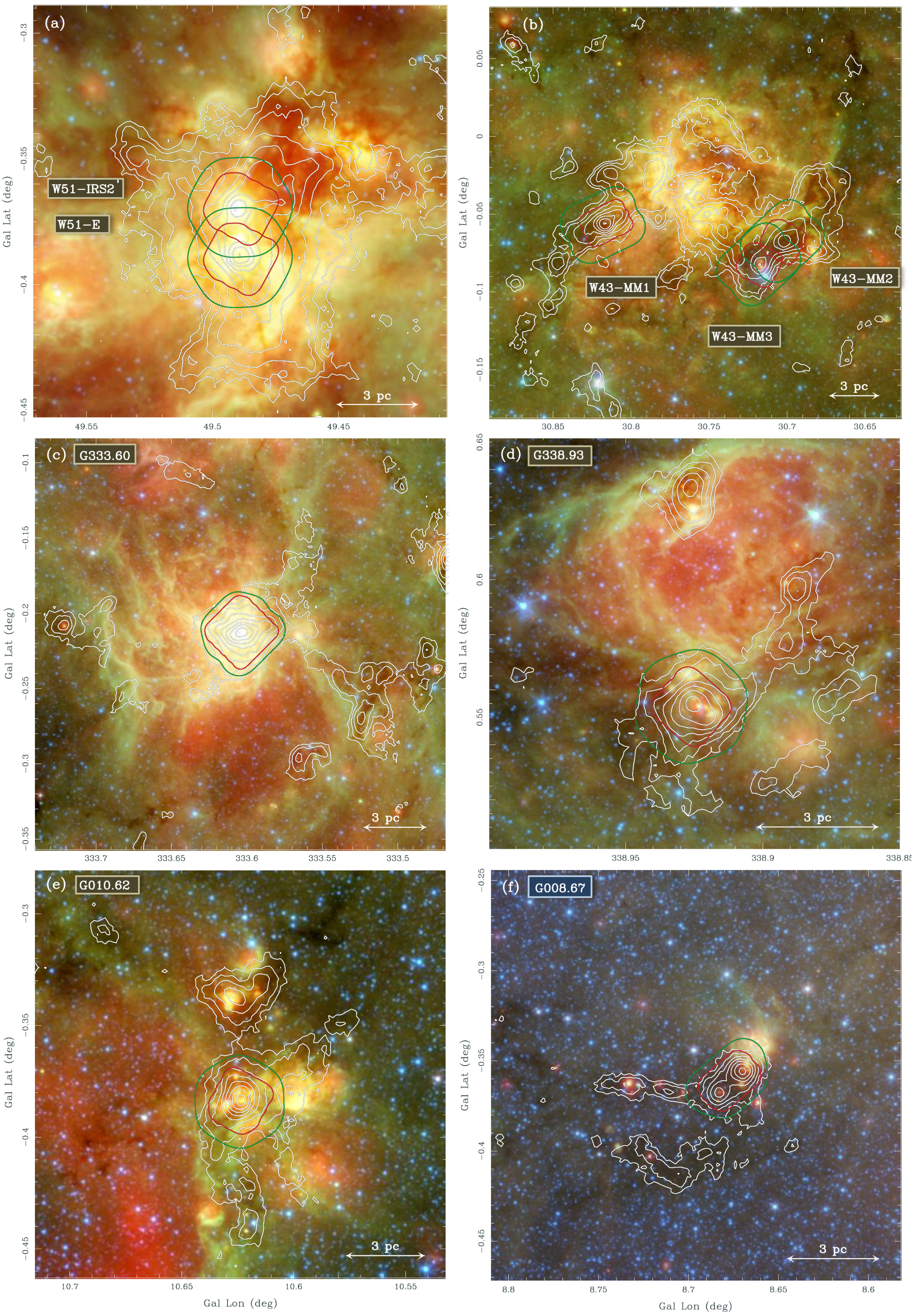
Figure 1: Overview of the surroundings of the ALMA-IMF protocluster clouds, ordered by decreasing mass of their central clump (Col. 9 of Table 1): W51-E and W51-IRS2 (in a), W43-MM1, W43-MM2, and W43-MM3 (in b), G333.60 (in c), G338.93 (in d), G010.62 (in e), and G008.67 (in f). ATLASGAL $870\;\mu$m emission contours (logarithmically spaced from 0.45 Jy/beam to 140 Jy/beam with a $19.2\arcsec$ beam) are overlaid on Spitzer three-color images (red represents MIPS $24\;\mu$m, green GLIMPSE $8\;\mu$m, and blue GLIMPSE $3.6\;\mu$m). The green and red contours outline the primary beam response of the ALMA 12 m array mosaics down to $15\%$ at 3 mm and 1.3 mm, respectively. A 3 pc scale bar is shown in the lower-right corner of each image.

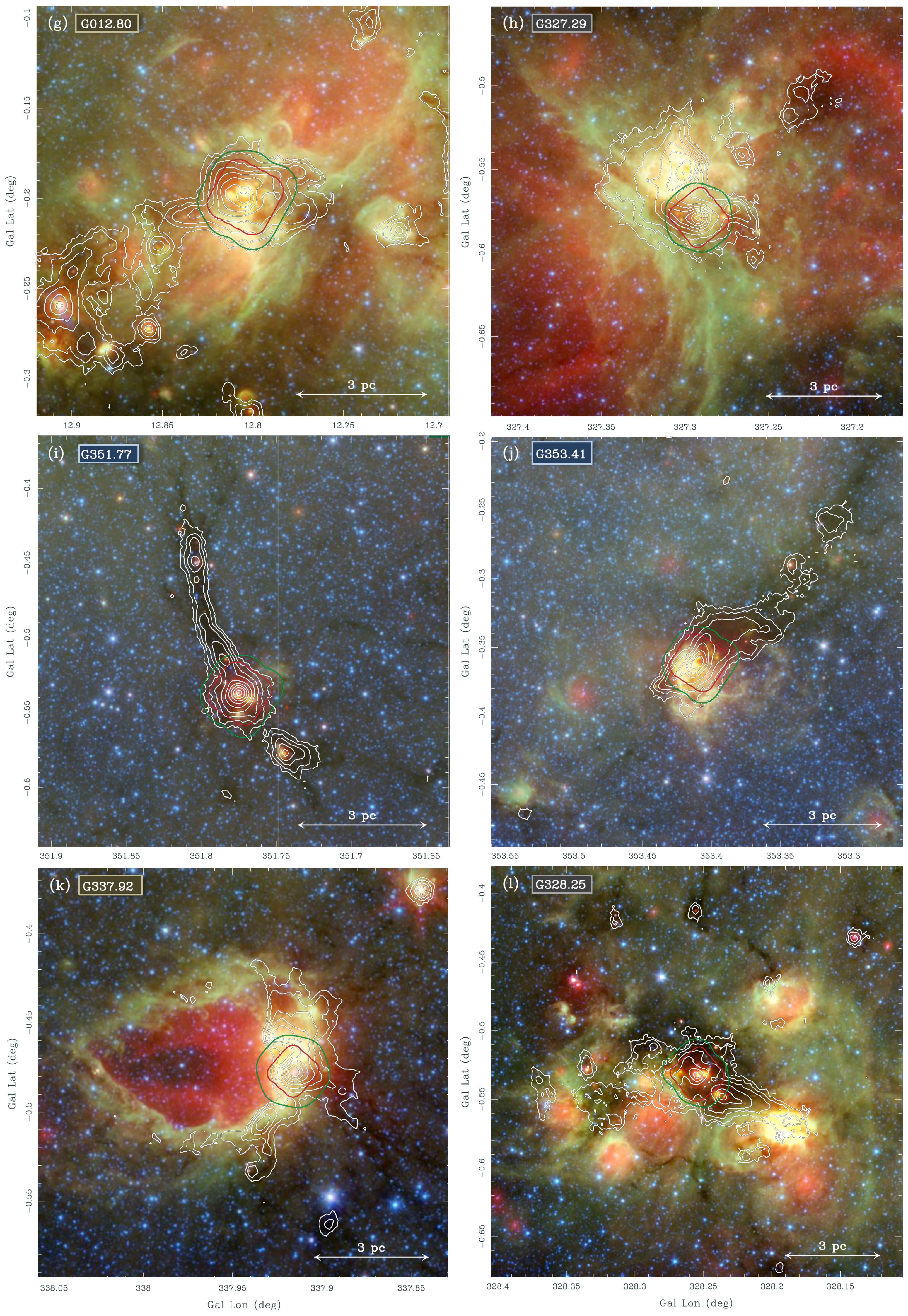
Figure 1: (Continued) Overview of the surroundings of the protocluster clouds G012.80 (in g), G327.29 (in h), G351.77 (in i), G353.41 (in j), G337.92 (in k), and G328.25 (in l).

[c] Protocluster RA¹ Dec¹ $V_{\rm LSR}$¹ $d$ Ref. Evolutionary FWHM${}_{\rm 870\,\mu m}^{\rm clump}$⁴ $M_{\rm 870\,\mu m}^{\rm clump}$⁴ cloud name¹ [ICRS] [km s^-1] [kpc] papers² stage³ [pc] [$\times 10^{3}\leavevmode\nobreak\ \mbox{$M_{\odot}$}$] W51-E 19:23:44.18 $+$14:30:29.5 $+55$ 5.4$\pm 0.3$ (1) IR-bright 0.41 $10.4$ W43-MM1 18:47:47.00 $-$01:54:26.0 $+97$ 5.5$\pm 0.4$ (2) IR-quiet 0.47 $7.0$ G333.60 16:22:09.36 $-$50:05:58.9 $-47$ 4.2$\pm 0.7$ (3) IR-bright 0.58 $5.4$ W51-IRS2 19:23:39.81 $+$14:31:03.5 $+55$ 5.4$\pm 0.3$ (1) IR-bright 0.39 $4.8$ G338.93 16:40:34.42 $-$45:41:40.6 $-62$ 3.9$\pm 1.0$ (3) IR-quiet 0.58 $4.5$ G010.62 18:10:28.84 $-$19:55:48.3 $-2$ 4.95$\pm 0.5$ (4) IR-bright 0.42 $4.2$ W43-MM2 18:47:36.61 $-$02:00:51.1 $+97$ 5.5$\pm 0.4$ (2) IR-quiet 0.57 $4.2$ G008.67 18:06:21.12 $-$21:37:16.7 $+37.6$ 3.4$\pm 0.3$ (3) IR-quiet 0.33 $1.9$ G012.80 18:14:13.37 $-$17:55:45.2 $+37$ 2.4$\pm 0.2$ (5) IR-bright 0.32 $1.7$ G327.29 15:53:08.13 $-$54:37:08.6 $-45$ 2.5$\pm 0.5$ (3) IR-bright 0.16 $1.4$ W43-MM3 18:47:41.46 $-$02:00:27.6 $+97$ 5.5$\pm 0.4$ (2) IR-bright 0.47 $1.1$ G351.77 17:26:42.62 $-$36:09:20.5 $-3$ 2.0$\pm 0.7$ (6) IR-bright 0.16 $1.0$ G353.41 17:30:26.28 $-$34:41:49.7 $-17$ 2.0$\pm 0.7$ (6) IR-bright 0.30 $0.9$ G337.92 16:41:10.62 $-$47:08:02.9 $-40$ 2.7$\pm 0.7$ (6) IR-bright 0.20 $0.8$ G328.25 15:57:59.68 $-$53:58:00.2 $-43$ 2.5$\pm 0.5$ (3) IR-quiet 0.21 $0.5$

Table 1: ALMA-IMF targets, a representative sample of massive protoclusters in the Milky Way.

• Protocluster name, central position of the mosaics, and velocity at rest used for the ALMA-IMF observations. The Galactic coordinates of the associated ATLASGAL clumps are given in Table 6. The $V_{\rm LSR}$ values are taken from the high-density gas studies by Wienen et al. (2015) and Ginsburg et al. (2015) for W51, Nguyen-Luong et al. (2013) for W43, and Immer et al. (2014) for G012.80. The phase center of W43-MM1 in the pilot study is 18:47:46.50, -01:54:29.5.

• References for the distance to the Sun: (1) Sato et al. (2010); (2) Zhang et al. (2014); (3) Csengeri et al. (2017); (4) Sanna et al. (2014); (5) Immer et al. (2013); (6) this paper.

• Evolutionary stage of the ATLASGAL clump, as classified by Csengeri et al. (2017): IR-bright or IR-quiet (see Sect. 2.2).

• Size and mass of the ATLASGAL clump, as defined by Csengeri et al. (2017), located at the center of the ALMA-IMF clouds, whose area and mass are given in Table 4. Mass estimates assume $\mbox{$T_{\rm dust}$}=20$ K and 30 K for the IR-quiet and IR-bright sources, respectively. Sizes correspond to the geometric mean of the beam-deconvolved major and minor FWHM axes of Gaussian fits made in Csengeri et al. (2014).

2 ALMA-IMF targets

In an effort to investigate statistically the richest protoclusters of the Milky Way, we compiled a list of 15 massive clouds. Table 1 lists their adopted names, the coordinates used as phase center, and velocity in the kinematic Local Standard of Rest. Figure 1 illustrates their surroundings with overlays of the mid-infrared Spitzer emission associated with the heating of luminous sources (Benjamin et al. 2003; Carey et al. 2009) and the ATLASGAL submillimeter emission tracing the cloud gas (Schuller et al. 2009). As one of the main goals of the ALMA-IMF Large Program is to create large catalogs of protocluster cores, we focused on massive clouds selected from Csengeri et al. (2017), which have sizes of a few parsecs and can be properly imaged by ALMA with an angular resolution down to a few thousand au (see Sect. 2.1). We then selected a representative sample of half (i.e., 15) of these protoclusters spanning a range of evolutionary stages (see Sect. 2.2).

2.1 The most massive protocluster clouds of the Milky Way

From the catalog of Csengeri et al. (2017), which contains the 200 most massive APEX/ATLASGAL clumps, we identified the most massive protocluster clouds of the Milky Way, whose core content can be characterized by ALMA (see Table 6 and Fig. 9). In order to reach an angular resolution of a couple of thousand au and a subsolar mass sensitivity with reasonable ALMA integration times, while reaching the exceptional W43 mini-starburst region at 5.5 kpc (Nguyen Luong et al. 2011), we applied a distance-limited criterion of $d\leq 5.5\leavevmode\nobreak\ \mbox{kpc}$. With this upper limit for the distance and avoiding Galactic longitudes toward the Galactic center ($355\degree<l<5\degree$), we further excluded regions at larger distances that would require long integration times and are already the focus of dedicated ALMA studies (e.g., Galván-Madrid et al. 2013; Sánchez-Monge et al. 2017). On the other hand, setting a lower distance limit of 2 kpc allows us to more easily observe the entire extent of the parsec-size clouds with ALMA mosaics. Furthermore, massive cloud complexes at lower distances (¡2 kpc), including Cygnus X, NGC 6334, M 17, and Orion, have already been extensively studied by, for example, the Herschel/HOBYS key program (Motte et al. 2010) and already revealed the nearest sites of high-mass star and cluster formation (e.g., Bontemps et al. 2010; Ohashi et al. 2016; Louvet et al. 2019; Sadaghiani et al. 2020; Fischer et al. 2020).

As our aim is to focus on the densest $\sim$1 pc size clouds hosting the ATLASGAL clumps, we selected the ATLASGAL sources of Csengeri et al. (2017) that have an integrated $870\;\mu$m flux larger than 25 Jy. This threshold, which is used to define the most massive protoclusters, corresponds to five times that used in Csengeri et al. (2017) and leads to a list of 28 potential targets. This flux threshold ensures a minimum mass of $\sim$400$-3\,000\leavevmode\nobreak\ \mbox{$M_{\odot}$}$ for the densest regions in the massive protoclusters at distances of 2-5.5 kpc, and assuming appropriate values for our sample of $\mbox{$T_{\rm dust}$}=25$ K and $\kappa_{\rm 870\,\mu m}=\rm 0.0185\leavevmode\nobreak\ cm^{2}\,g^{-1}$ in Section 2.2 (see Sect. 2.2). Among these 28 massive protoclusters, we find W51-E, W51-IRS2, W43-MM1, and W43-MM2 previously identified as extremely massive and active mini-starburst clumps (Motte et al. 2003; Ginsburg et al. 2012). Furthermore, we add two sources to this list: the ATLASGAL source W43-MM3 to cover the W43-MM2&MM3 mini-starburst ridge, which is suspected to host an extreme protocluster (Nguyen-Luong et al. 2013), and G328.25-0.58, which is the most massive, young protocluster of Csengeri et al. (2017) that exhibits at its center a single high-mass protostar (Csengeri et al. 2018). The catalog of the 30 selected massive clumps is given in Table 6. Their Galactic coordinates, evolutionary stage, and integrated flux at $870\;\mu$m are taken from Csengeri et al. (2017). We also include a list of ALMA projects that previously targeted these protoclusters, the name of the molecular complex hosting them, and their distance to the Sun in Table 6.

Ten of the massive clumps of Table 6 have a distance measured by trigonometric parallaxes using masers (Sato et al. 2010; Immer et al. 2013; Sanna et al. 2014; Reid et al. 2014; Zhang et al. 2014). The distances for the remaining sources were estimated by Csengeri et al. (2017) using kinematic distance estimates, associations with cloud complexes, and mid-infrared absorption features (as done by Moisés et al. 2011; Wienen et al. 2015). These distance estimates are subject to uncertainties, such as the Galactic rotation curve and association with the near or far kinematic distance solutions. Improvements can only be expected when parallax distances are available using either weaker masers or, for the closest clumps, Gaia measurements. We here modify the distances of three ATLASGAL clumps of Table 6 using recent improvements made by the BeSSeL project (see Reid et al. 2014). With its revised kinematic distance calculator, the two relatively nearby clumps, G351.77 and G353.41, both have almost equally probable distance solutions of $\sim$1.3 kpc and $\sim$2.7 kpc. Given that the cloud gas between these two clumps presents a velocity continuity, G353.41-0.36 and G351.41-0.54 are probably part of the same complex and we adopted the average distance of $\sim$2.0 kpc, with a dispersion of $\pm 0.7$ kpc, for both clumps. Moreover, we updated the distance of the G337.92-0.48 clump to $2.7\pm 0.3$ kpc, following that given by the BeSSeL calculator.

2.2 A representative sample of 15 massive protoclusters at various evolutionary stages

We extracted from Table 6 a smaller sample of clouds, covering a range of evolutionary stages. Csengeri et al. (2017) classified ATLASGAL clumps as either IR-bright or IR-quiet, based on their fluxes at mid-IR wavelengths. Initially proposed by Motte et al. (2007), this classification has been adapted, in Csengeri et al. (2017), to use a flux threshold of 289 Jy at $22\;\mu$m and $d=1$ kpc, scaling it to the distances of the sources and extrapolating fluxes from the Wide-field Infrared Survey Explorer (WISE) or the Multiband Imaging Photometer for Spitzer (Spitzer/MIPS) observatories. This classification is expected to distinguish between clumps hosting faint infrared (IR-quiet) sources corresponding to deeply embedded, Class-0-like, high-mass protostars (e.g., Bontemps et al. 2010) and those with luminous infrared (IR-bright) objects. The latter are either ultra-compact H ii regions or clumps hosting evolved protostars, referred to as high-mass protostellar objects (HMPOs, see Beuther et al. 2002) or massive young stellar objects (MYSOs, see Lumsden et al. 2013). The IR-quiet/IR-bright classification makes it possible to follow the evolution from cold to warm cloud structures (e.g., Motte et al. 2018a), where cold stages are sometimes referred to as infrared dark clouds (IRDCs), even if they host various stages of low- and high-mass star formation (e.g., Peretto et al. 2013).

Table 6 contains only seven IR-quiet clumps, which exclusively populate the low $870\,\mu$m flux end of the sample distribution. IR-quiet protoclusters, however, as they are not yet significantly impacted by stellar feedback, probably represent the early stage during which it should be easier to study the CMF and its variation with cloud properties. We therefore rebalanced the sample of massive protocluster clouds to be used for the ALMA-IMF Large Program by systematically selecting the top seven, IR-bright, clumps of Table 6, but favoring IR-quiet clumps among the remaining 21 clumps.

To complement this selection, we first chose to cover all of the extreme protoclusters, which lie in the two exceptional, and relatively distant, cloud complexes W51 and W43: W51E, W51-IRS2, W43-MM1, W43-MM2, and W43-MM3. For the remaining molecular cloud complexes, we instead chose to observe only one protocluster per complex to sample various parts of the Milky Way. In the RCW106 and G327 complexes, we therefore only selected the brightest ATLASGAL clump, which happened to be IR-bright. In total, we selected for the ALMA-IMF survey five (out of seven, $71\%$) and ten (out of 23, $43\%$) of the IR-quiet and IR-bright clumps from Table 6, respectively.

Table 1 lists the 15 protocluster clouds selected for the ALMA-IMF Large Program, which constitute a representative and well-balanced sample of the most massive protoclusters in the Milky Way. It gives their distance to the Sun, evolutionary stage, and the size and mass of their central clump, FWHM${}_{\rm 870\,\mu m}^{\rm clump}$ and $M_{\rm 870\,\mu m}^{\rm clump}$, the latter being used here to order the cloud sample. In this final selection, the 15 massive protoclusters are located at $2-5.5$ kpc with a mean distance of 3.9 kpc. Since the $870\,\mu$m fluxes mainly correspond to thermal dust emission, which is largely optically thin, the clump mass is computed from the integrated fluxes, $S^{\rm int}_{\rm 870\,\mu m}$ listed in Table 6, assuming a mass-averaged dust temperature and a distance to the Sun. We used the following equation, and provide here a numerical application whose dependence on each physical variable is given, for simplicity, in the Rayleigh-Jeans approximation:

$$M^{\rm clump}_{\rm 870\,\mu m} = \frac{S^{\rm int}_{\rm 870\,\mu m}\;d^{2}}{\kappa_{\rm 870\,\mu m}\;B_{\rm 870\,\mu m}(\mbox{$T_{\rm dust}$})}$$

$$\approx 84\ \mbox{$M_{\odot}$}\times\left(\frac{S^{\rm int}_{\rm 870\,\mu m}}{\mbox{1\leavevmode\nobreak\ Jy}}\right)\left(\frac{d}{\mbox{3.9\leavevmode\nobreak\ kpc}}\right)^{2}$$

$$\times\left(\frac{\kappa_{\rm 870\,\mu m}}{\rm 0.0185\,cm^{2}\,g^{-1}}\right)^{-1}\left(\frac{\mbox{$T_{\rm dust}$}}{\rm 20\leavevmode\nobreak\ K}\right)^{-1},$$

where $B_{\rm 870\,\mu m}(\mbox{$T_{\rm dust}$})$ is the Planck function for a dust temperature $T_{\rm dust}$, $d$ is the distance of ALMA-IMF protoclusters, and $\kappa_{\rm 870\,\mu m}$ is the dust opacity per unit (gas $+$ dust) mass at $870\,\mu$m. The adopted dust opacity, $\kappa_{\rm 870\,\mu m}=0.0185\,\rm cm^{2}\,g^{-1}$, follows the prescriptions by Ossenkopf & Henning (1994) and assumes a gas-to-dust mass ratio of 100. We adopted dust temperatures of $\mbox{$T_{\rm dust}$}=20$ K and 30 K for the IR-quiet and IR-bright regions, respectively (see also Sect. 4.1 for more discussion). These are the mean temperatures of the brightest ATLASGAL sources as measured in NH₃ (Wienen et al. 2012, 2018) in agreement with dust temperatures of König et al. (2017). In these 15 massive protoclusters, the mass of the central clump ranges from $500\leavevmode\nobreak\ \mbox{$M_{\odot}$}$ to $1\times 10^{4}\leavevmode\nobreak\ \mbox{$M_{\odot}$}$.

Figure 1 illustrates the IR-quiet versus IR-bright evolutionary stage of these protocluster clouds. The five IR-quiet protocluster clouds are all observed as strong extended ATLASGAL cloud structures associated with extinction patterns at mid-infrared wavelengths (see Figs. 1b, d, f, l). In contrast, the ten IR-bright protoclusters emit at near- to mid-infrared wavelengths, either weakly (see Figs. 1b, i–j) or more strongly (see Figs. 1a, c, e, g–h, k).

Beyond their different evolutionary stages, the targeted protoclusters may represent different conditions for cluster formation in the galactic disk of the Milky Way. The five protoclusters in the W43 and W51 cloud complexes are among the most active star-forming regions of the Milky Way. W43 is located at the end of the Galactic bar and W51 could be a massive cloud compressed by Galactic motions along the Perseus arm (Nguyen Luong et al. 2011; Ginsburg et al. 2015). Seven other ALMA-IMF clouds could be under the influence of massive stellar clusters. Each of the G010.62, G337.92, and G338.93 clouds is indeed located at the periphery of a large bubble, presumably excited by OB stars, and the G333.60, G327.29, G328.25, and G012.80 clouds are found in complex networks of such bubbles (see Fig. 1). In contrast, the G008.67, G351.77, and G353.41 clouds seem more isolated, without obvious interaction with massive stellar clusters or Galactic motions.

Table 2: Observational data summary of the 12 m array continuum images of ALMA-IMF protoclusters.

[c] 1.3 mm (Band 6) 3 mm (Band 3) Protocluster Imaged FOV¹ Resolution² $\sigma$(cleanest)³ $\sigma$(bsens)³ LAS_10%⁴ Imaged FOV¹ Resolution² $\sigma$(cleanest)³ $\sigma$(bsens)³ LAS_10%⁴ cloud name [$\arcsec\times\arcsec$] [$\arcsec\times\arcsec$] [$\mathrm{mJy\,beam^{-1}}$] [$\arcsec$] [$\arcsec\times\arcsec$] [$\arcsec\times\arcsec]$ [$\mathrm{mJy\,beam^{-1}}$] [$\arcsec$] W51-E $100\times 90$ $0.35\times 0.27$ 0.17 0.16 5.0 $150\times 160$ $0.29\times 0.26$ 0.055 0.035 6.3 W43-MM1 $117\times 53$ $0.50\times 0.35$ 0.19 0.18 4.6 $190\times 150$ $0.56\times 0.33$ 0.051 0.038 4.8 G333.60 $143\times 143$ $0.56\times 0.51$ 0.11 0.12 5.8 $190\times 180$ $0.46\times 0.44$ 0.070 0.047 10 W51-IRS2 $92\times 98$ $0.50\times 0.44$ 0.097 0.076 6.1 $160\times 150$ $0.28\times 0.27$ 0.061 0.061 9.6 G338.93 $86\times 92$ $0.56\times 0.51$ 0.17 0.16 5.5 $152\times 160$ $0.40\times 0.38$ 0.068 0.044 11 G010.62 $98\times 90$ $0.53\times 0.41$ 0.083 0.082 5.2 $150\times 160$ $0.39\times 0.32$ 0.051 0.051 9.4 W43-MM2 $90\times 98$ $0.52\times 0.41$ 0.075 0.063 5.5 $190\times 150$ $0.30\times 0.24$ 0.037 0.024 8.1 G008.67 $132\times 87$ $0.72\times 0.59$ 0.37 0.20 5.9 $190\times 125$ $0.51\times 0.40$ 0.094 0.080 10 G012.80 $132\times 132$ $1.09\times 0.70$ 0.65 0.74 6.6 $190\times 180$ $1.48\times 1.26$ 0.21 0.24 9.9 G327.29 $105\times 109$ $0.69\times 0.62$ 0.36 0.32 5.5 $160\times 152$ $0.43\times 0.37$ 0.13 0.075 10 W43-MM3 $100\times 90$ $0.51\times 0.43$ 0.061 0.063 5.7 $190\times 150$ $0.41\times 0.29$ 0.031 0.028 8.2 G351.77 $132\times 132$ $0.89\times 0.67$ 0.42 0.31 6.2 $190\times 180$ $1.52\times 1.30$ 0.26 0.12 15 G353.41 $131\times 131$ $0.93\times 0.66$ 0.42 0.40 6.2 $190\times 180$ $1.46\times 1.27$ 0.18 0.17 10 G337.92 $92\times 86$ $0.61\times 0.48$ 0.22 0.23 5.6 $160\times 152$ $0.45\times 0.38$ 0.070 0.051 11 G328.25 $120\times 120$ $0.62\times 0.47$ 0.37 0.29 4.9 $160\times 180$ $0.62\times 0.44$ 0.087 0.076 7.5

• Field of view (FOV) corresponding to the combined primary beam of the 1.3 mm and 3 mm mosaics, down to $15\%$ of the peak sensitivity.

• Angular resolution resulting from a tclean process with the Briggs robust parameter robust=0.

• Noise level measured in the bsens and cleanest 12 m array images at 1.3 mm and 3 mm.

• The maximum recoverable scale of the 12 m array, often called the largest angular scale (LAS), is estimated for each 1.3 m and 3 mm images as the 10^th percentile of the baseline lengths of 12 m array data (see Figs. 5–7 of Ginsburg et al. in press.).

[c]

Table 3: Spectral setup of the ALMA-IMF Large Program.

ALMA	Spectral	Frequency	Bandwith	Resolution		Main spectral lines
band	window	[GHz]	[MHz]	[kHz]	[km s-1]
Band 6	SPW0	216.200	234	244	0.34	DCO+ (3-2), CH3OCHO, OC33S (18-17), HCOOH
	SPW1	217.150	234	282	0.39	SiO (5-4), DCN (3-2), 13CH3OH, CH3OCH3
	SPW2	219.945	117	282	0.38	SO (6-5), H${}_{2}^{13}$CO (31,2-21,1), CH3OH
	SPW3	218.230	234	244	0.33	H2CO (3-2), O13CS (18-17), HC3N (24-23), CH3OCHO
	SPW4	219.560	117	244	0.33	C18O (2-1), C2H5CN
	SPW5	230.530	469	969	1.3	CO (2-1), CH3CHO, CH3OH, C2H3CN, C2H5OH
	SPW6	231.280	469	488	0.63	13CS (5-4), N2D+ (3-2), OCS (19-18), CH3CHO, CH3OH,
						CH${}_{3}^{18}$OH, C2H5CN
	SPW7	232.450	1875	1130	1.5	H30$\alpha$, CH3CHO, CH3OH, CH3OCHO, C2H5OH, C2H5CN,
						CH3OCH3, CH3COCH3, 13CH3CN (13-12), H2C34S (71,7-61,6), HC(O)NH2
Band 3	SPW0	93.1734	117	71	0.23	N2H+ (1-0), CH3OH
	SPW1	92.2000	938	564	1.8	CH3CN (5-4), H41$\alpha$, CH313CN, 13CS (2-1), 13CH3OH, CH3OCHO
	SPW2	102.600	938	564	1.6	CH3CCH (6-5), CH3OH, H2CS,C2H5CN, C2H5OH, CH3NCO
	SPW3	105.000	938	564	1.6	H2CS, CH3OH, C2H3CN, C2H5OH, CH3OCH3

[c] Protocluster Imaged areas¹ $S^{\rm cloud}_{\rm 870\,\mu m}$² $M^{\rm cloud}_{\rm 870\,\mu m}$³ $S^{\rm cloud}_{\rm 1.3\,mm}$ $\Sigma^{\rm free-free}_{\rm H41\alpha}$ ⁴ Refined cloud name [$\mbox{pc}\times\mbox{pc}$] within $A_{\rm 1.3\,mm}$ $/S^{\rm cloud}_{\rm 3\,mm}$ over $A_{\rm 1.3\,mm}$ evolutionary $A_{\rm 1.3\,mm}$ $A_{\rm 3\,mm}$ [Jy] [$\times 10^{3}\leavevmode\nobreak\ \mbox{$M_{\odot}$}$] over $A_{\rm 1.3\,mm}$ [$\rm Jy\,pc^{-2}$] stage⁵ W43-MM1 $3.1\times 2.3$ $5.1\times 4.0$ 80.3 13.4 13 0.005 IR-quiet $=$ Y W43-MM2 $2.6\times 2.4$ $5.1\times 4.0$   69.6 11.6 15 0.009 IR-quiet $=$ Y G338.93 $1.6\times 1.6$ $2.9\times 2.8$   84.6 7.1 7.2 0.02 IR-quiet $=$ Y G328.25 $1.4\times 1.4$ $2.2\times 1.9$   73.2 2.5 8.3 0.03 IR-quiet $=$ Y G337.92 $1.2\times 1.1$ $2.1\times 2.0$   63.3 2.5 5.8 0.04, faint H ii IR-bright $\rightarrow$ Y G327.29 $1.3\times 1.3$ $1.9\times 1.8$ 147.9 5.1 11 0.1, faint H ii IR-bright $\rightarrow$ Y G351.77 $1.3\times 1.3$ $1.8\times 1.7$ 158.7 2.5 8.3 0.2, UCH ii IR-bright $\rightarrow$ I G008.67 $2.2\times 1.4$ $3.1\times 2.1$   66.5 3.1 3.2 0.6, UCH ii IR-quiet $\rightarrow$ I W43-MM3 $2.7\times 2.4$ $5.1\times 4.0$   43.2 5.2 2.2 0.2, UCH ii IR-bright $\rightarrow$ I W51-E $2.6\times 2.4$ $4.2\times 3.9$ 278.9 32.7 2.2 1, two HCH ii $+$ H ii IR-bright $\rightarrow$ I G353.41 $1.3\times 1.3$ $1.8\times 1.7$ 153.4 2.5 1.9 0.7, UCH ii $+$ H ii IR-bright $\rightarrow$ I G010.62 $2.3\times 2.2$ $3.8\times 3.6$   87.3 6.7 1.8 2, two H ii IR-bright $=$ E W51-IRS2 $2.6\times 2.4$ $4.2\times 3.9$ 224.4 20.6 1.4 2, two H ii IR-bright $=$ E G012.80 $1.5\times 1.5$ $2.2\times 2.1$ 255.4 4.6 1.1 7, H ii IR-bright $=$ E G333.60 $2.9\times 2.9$ $3.9\times 3.7$ 216.3 12.0 0.8 5, H ii IR-bright $=$ E

Table 4: Main characteristics (size and mass) of the massive protocluster clouds imaged by ALMA-IMF and their evolutionary stage.

• Physical areas encompassing the combined primary beam of the 1.3 mm and 3 mm mosaics, down to $15\%$. These areas define the cloud sizes.

• Integrated flux density at 870$\,\mu$m measured on the ATLASGAL images (Schuller et al. 2009) within the area of the 1.3 mm ALMA images (Col. 2).

• Cloud mass computed from the $870\,\mu$m integrated flux (Col. 4) assuming $\kappa_{\rm 870\,\mu m}=\rm 0.0185\leavevmode\nobreak\ cm^{2}\,g^{-1}$ and using $\mbox{$T_{\rm dust}$}=20$ K, 25 K and 30 K for the Young, Intermediate, and Evolved regions (see Col. 8), respectively.

• Flux surface density of the free-free emission at 92.034 GHz, estimated from the integrated flux of the H41$\alpha$ recombination line. Spatial distribution of the ionized gas: HCH ii and UCH ii consist of $<$0.05 pc and $\sim$0.1 pc bubbles of ionized gas, respectively; H ii are larger regions of ionized gas with a non-spherical structure, some are faint H ii regions (see Sect. 4.1 and Motte et al. 2018a).

• Classification of the ALMA-IMF protocluster clouds: Young (Y), Intermediate (I), and Evolved (E). Their evolutionary stage is refined from that of Csengeri et al. (2017) by measuring their 1.3 mm to 3 mm flux ratio (Col. 6) and their estimated free-free emission flux density (Col. 7). We assume that IR-quiet and IR-bright ATLASGAL clumps are associated with Young and Evolved clouds, respectively. Any evolution of this classification is discussed in Sect. 4.1 and indicated here by an arrow.

3 Observations and data reduction

The ALMA-IMF Large Program (#2017.1.01355.L, PIs: Motte, Ginsburg, Louvet, Sanhueza) was set up following the pilot program #2013.1.01365.S. The ALMA-IMF Large Program images each of the 15 massive protocluster clouds of Table 1 both at 1.3 mm (ALMA Band 6) and 3 mm (Band 3). We here explain our observation strategy (see Sect. 3.1) and briefly discuss the resulting data set (see Sect. 3.2), which is described in more detail in Paper II (Ginsburg et al. in press.). Tables 2-3 give the mapping and spectral setups of the ALMA-IMF Large Program.

3.1 Observing strategy

To resolve the $\sim$2 000 au typical diameter of cores (Zhang et al. 2009; Bontemps et al. 2010; Palau et al. 2013) and image the $\sim$1$-8\leavevmode\nobreak\ \mbox{pc}^{2}$ protocluster cloud extent, 1.3 mm and 3 mm mosaics (shown in Figs. 1a–l and whose extent is listed in Table 2) were requested with $0.37\arcsec-0.95\arcsec$ synthesized beams depending on their distance (see Table 2).

We chose the 1.3 mm and 3 mm spectral bands primarily for their mostly optically thin emission in (massive) cores and their relatively well-defined dust opacities. The central frequencies of the ALMA-IMF bands are $\nu_{\textrm{B6}}=228.965$ GHz (1.3 mm) and $\nu_{\textrm{B3}}=100.713$ GHz (3 mm) (see Table D1 of Ginsburg et al. in press.), assuming a spectral index of $\alpha=3.5$ that corresponds to optically thin dust emission with an emissivity index of $\beta=1.5$, well suited for protostars (André et al. 1993; Juvela et al. 2015). According to Ossenkopf & Henning (1994) and assuming a gas-to-dust mass ratio of 100, the dust opacities per unit (gas $+$ dust) mass, recommended for cores, are $\kappa_{\rm 1.3\,mm}=\rm 0.01\leavevmode\nobreak\ cm^{2}\,g^{-1}$ and $\kappa_{\rm 3\,mm}=\kappa_{\rm 1.3\,mm}\times\left(\frac{\nu_{\textrm{B6}}}{\nu_{\textrm{B3}}}\right)^{-1.5}\simeq\rm 0.0034\leavevmode\nobreak\ cm^{2}\,g^{-1}$. The ALMA-IMF Large Program was designed to reach, for point-like cores, a gas mass sensitivity of $0.15\leavevmode\nobreak\ \mbox{$M_{\odot}$}$ ($3\,\sigma$) at 1.3 mm, for all protocluster clouds of Table 1 and over their whole extents (see Figs. 1a–l). Assuming optically thin dust emission, the above dust opacity, and a dust temperature of $20$ K, this requirement led to a large range of continuum sensitivity requests: $1\,\sigma=0.1-0.6$ mJy beam^-1 at 1.3 mm. To complete these 1.3 mm detections and correct them for a few optically thick (massive) cores, we aimed to reach a point mass sensitivity of $0.6\leavevmode\nobreak\ \mbox{$M_{\odot}$}$ ($3\,\sigma$) at 3 mm, corresponding to $1\,\sigma=0.03-0.18$ mJy beam^-1. As we show in Sect. 4.1, comparing the 1.3 mm and 3 mm continuum images allows us to distinguish thermal dust emitting sources, such as cloud filaments and cores, from free-free emitting sources associated with ionized gas of H ii regions.

The spectral setup chosen for the ALMA-IMF Large Program contains eight spectral windows at 228.4 GHz (1.3 mm) and four at 99.66 GHz (3 mm) (see Table 3). The 228.4 GHz setup is exactly the one used for the ALMA-IMF pilot project that targeted the W43-MM1 protocluster cloud (Nony et al. 2018, 2020). The main characteristics of these 12 spectral windows are given in Table 3, including the main lines they cover. ALMA-IMF has a particular focus on the N₂H⁺ (1-0), DCO⁺ (3-2), DCN (3-2), and C¹⁸O (2-1) lines intended to be used to trace gas mass inflows from the cloud to its cores (e.g., Csengeri et al. 2011a; Peretto et al. 2013; Henshaw et al. 2014; Chen et al. 2019; Álvarez-Gutiérrez et al. 2021). The ¹²CO (2-1), SiO (5-4), and SO (6-5) lines were chosen to trace protostellar outflows and shocks associated with protostellar accretion or cloud formation (e.g., Gusdorf et al. 2008; Sanhueza et al. 2013; Duarte-Cabral et al. 2014; Louvet et al. 2014; Li et al. 2020). Additionally, the ¹³CS (5-4) and N₂D⁺ (3-2) lines were chosen to estimate the core turbulence levels (e.g., Tan et al. 2013; Nony et al. 2018). As for the H41$\alpha$ and H30$\alpha$ recombination lines, they pinpoint H ii regions and allow for more robust gas mass estimates by accounting for free-free contamination of the millimeter fluxes (e.g., Liu et al. 2019). Molecules such as CH₃CN and CH₃CCH, can themselves be used to probe the gas temperature of hot cores and their envelopes or host cores, respectively. The lines of H₂CO, OCS, and other COMs (see Table 3) emitting in the 6.4 GHz noncontinuous bandwidth of the ALMA-IMF setup probe the physical and chemical conditions of hot cores, protostellar outflows, and shocks (e.g., Giannetti et al. 2017; Lefloch et al. 2017; Csengeri et al. 2019; Molet et al. 2019; Bonfand et al. 2019).

The ALMA-IMF Large Program was designed to provide sensitive continuum estimates through wide spectral windows: one $\sim$2 GHz window at 1.3 mm and three $\sim$1 GHz windows at 3 mm, with a velocity resolution of $\sim$1.5–1.8 km s^-1, also allowing the detection of broad hot core lines from COMs with confidence (e.g., Molet et al. 2019; Belloche et al. 2020; Olguin et al. 2021). The narrow spectral windows, except two at 1.3 mm, have a spectral resolution corresponding to $\sim$0.3 km s^-1 (see Table 3), suitable to follow the gas kinematics at the spectral resolution of the sonic line width (e.g., Henshaw et al. 2014; Chen et al. 2019). The two narrow spectral windows with a lower spectral resolution, $\sim$1.3 km s^-1 and $\sim$0.6 km s^-1, are customized to detect CO (2-1) outflows and to cover both the ¹³CS (5-4) and N₂D⁺ (3-2) lines, respectively.

The line sensitivity of the ALMA-IMF Large Program at 1.3 mm is driven by the need to detect $>$1 km s^-1 lines, such as ¹³CS (5-4) or N₂D⁺ (3-2), toward dust cores. With the requested 1.3 mm continuum sensitivity, $1\,\sigma=0.1-0.6$ mJy beam^-1, the expected noise level is $0.6-0.8$ K averaged within a spectral resolution element of 1 km s^-1. The targeted lines generally are ten to hundred times brighter (Tan et al. 2013; Nony et al. 2018), thus allowing their correct characterization in terms of line width. This sensitivity is also enough to detect outflowing material in CO (2-1) and SiO (5-4) around candidate protostellar sources (e.g., Nisini et al. 2007; Duarte-Cabral et al. 2013; Plunkett et al. 2013; Nony et al. 2020) and COMs tracing hot cores and shocks (e.g., Lefloch et al. 2017; Molet et al. 2019; Csengeri et al. 2019; Olguin et al. 2021). At 3 mm, the $1\sigma=0.03-0.18$ mJy beam^-1 continuum sensitivity leads to a sensitivity of $2-3$ K at 1 km s^-1 resolution. This allows N₂H⁺ (1-0) cubes to be sensitive down to the weakest filaments crossing the ALMA-IMF protoclusters (see, e.g., Fig. 7).

While compact structures, such as cores traced by their thermal continuum emission or hot cores identified by line forests, are marginally affected by interferometric artifacts, a proper analysis of molecular outflows and gas inflows would require combining ALMA 12 m array mosaics with 7 m array (Atacama Compact Array, ACA) data and, if possible, Total Power Array data (Zhang et al. 2016; Li et al. 2020; Hara et al. 2021). Therefore, the ALMA-IMF Large Program observed all the appropriate short spacing data that will allow correct analyses and provide the community with a complete and uniformly produced data set.

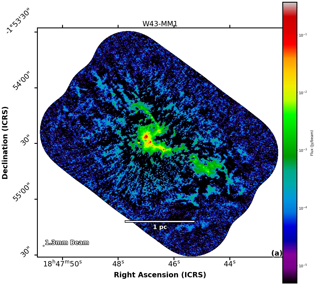
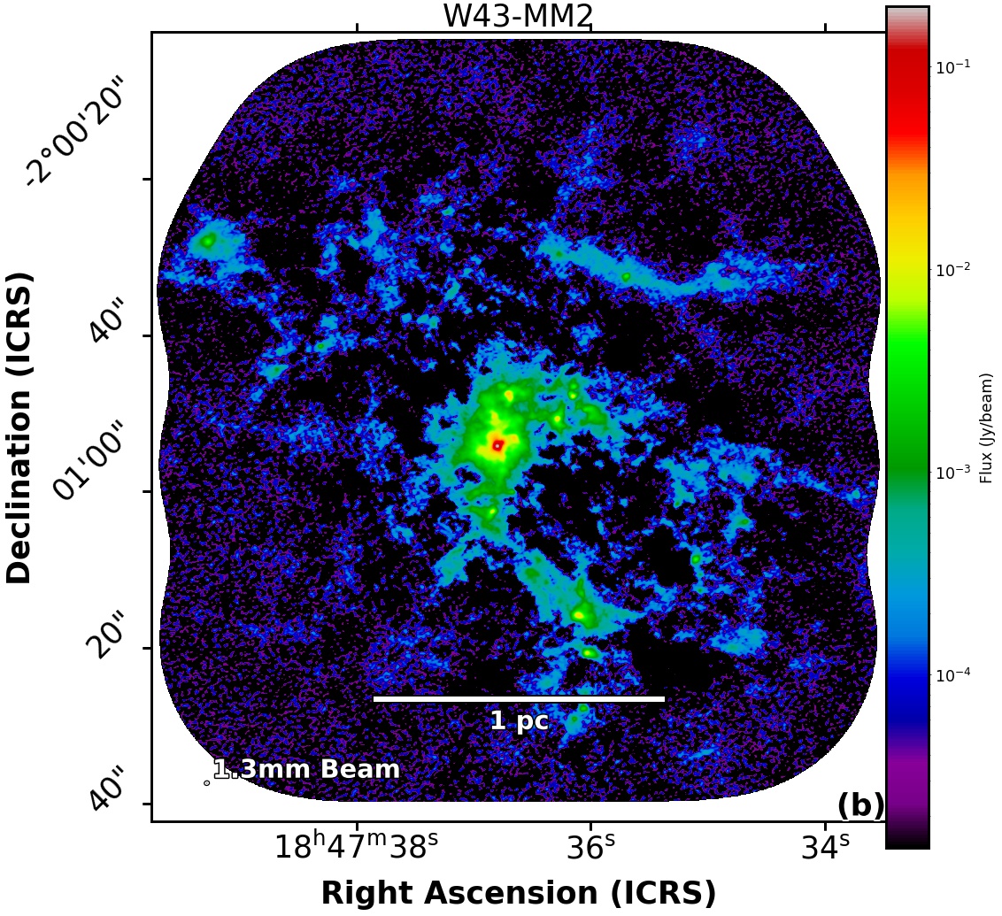
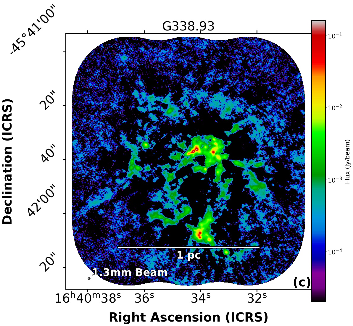
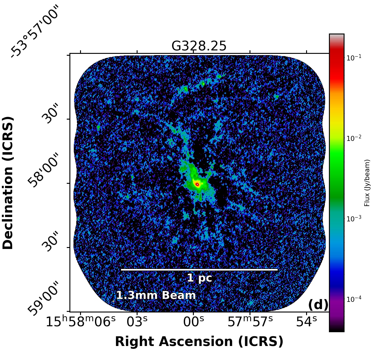
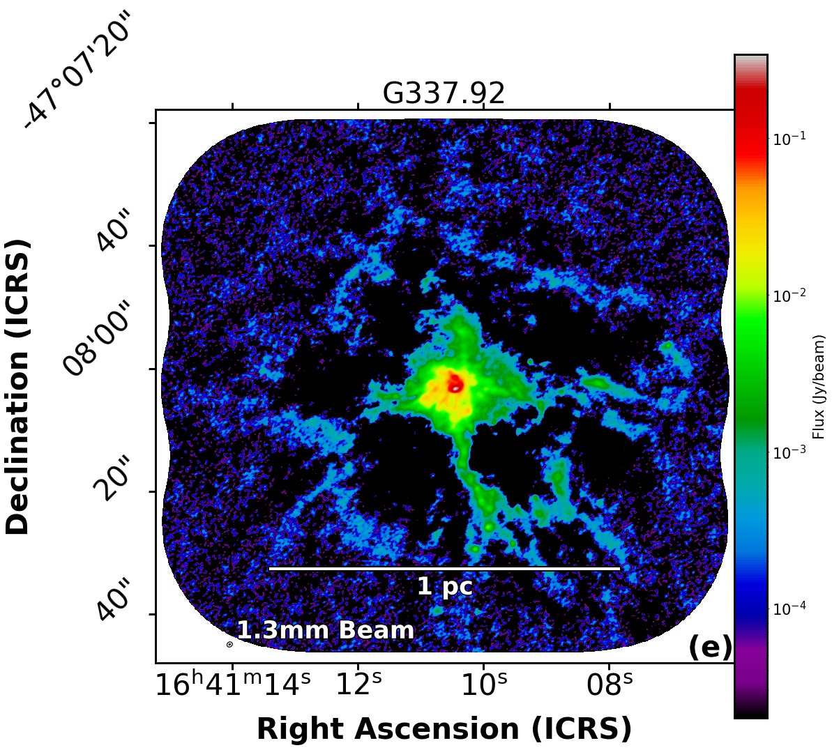
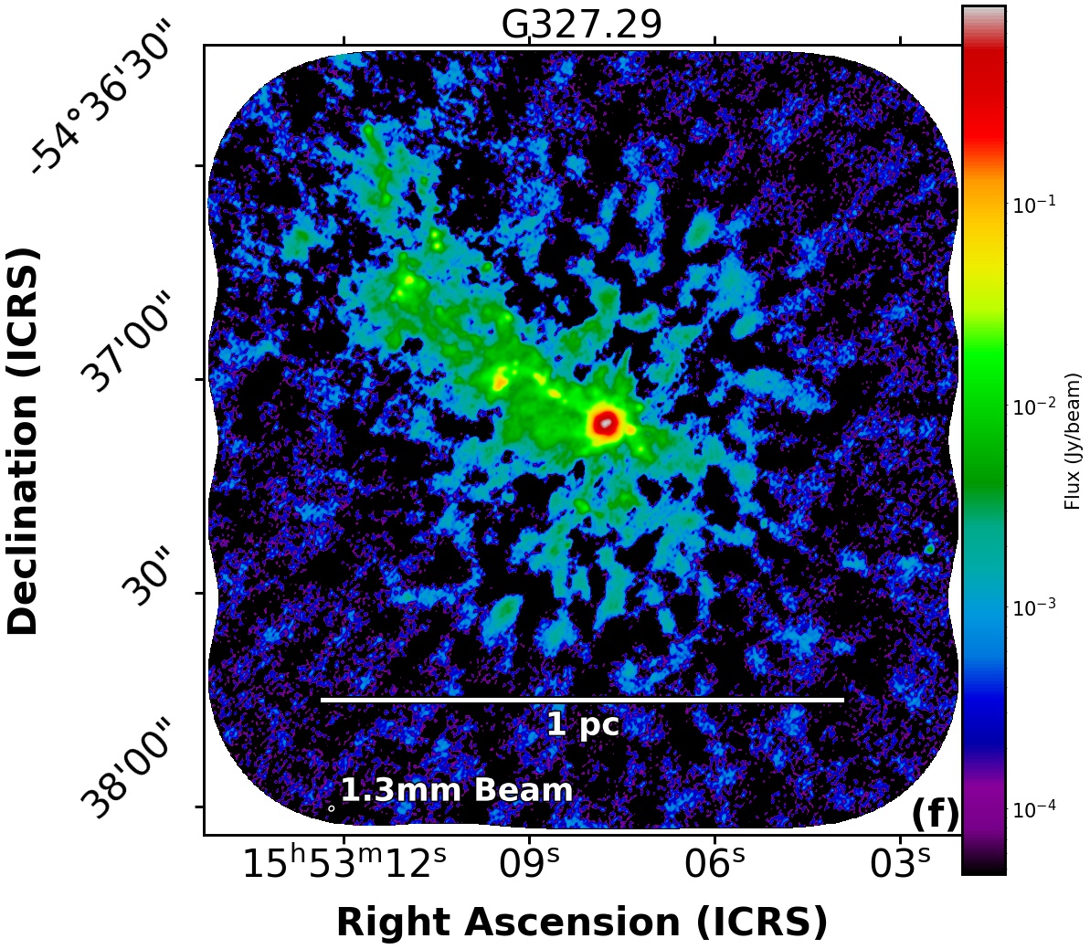
Figure 2: 1.3 mm continuum ALMA 12 m array images of the Young clouds: W43-MM1 (in a), W43-MM2 (in b), G338.93 (in c), G328.25 (in d), G337.92 (in e), and G327.29 (in f), plotted at the same physical scale.

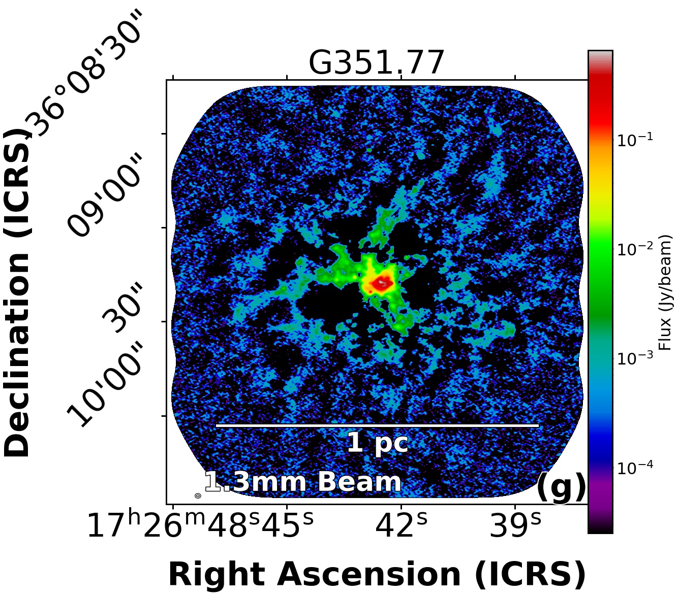
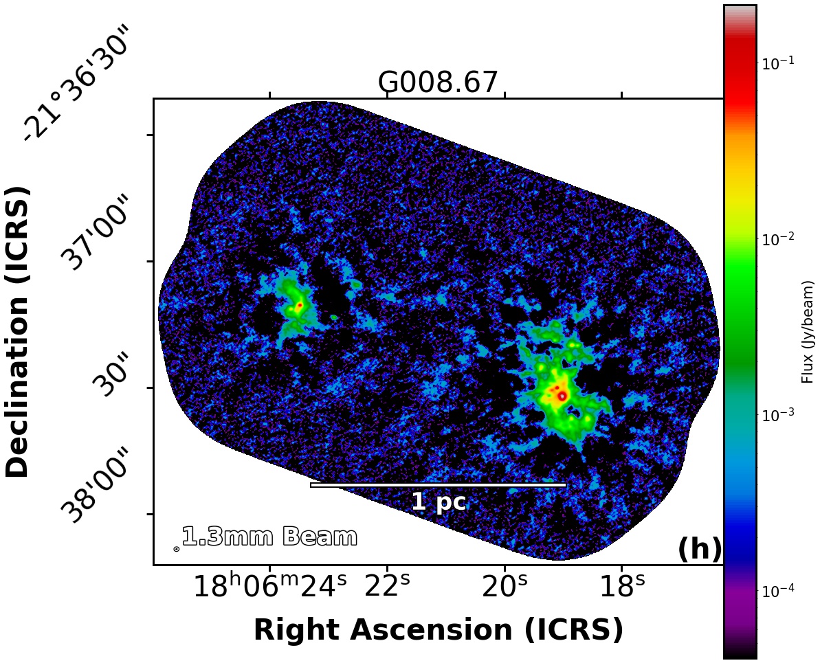
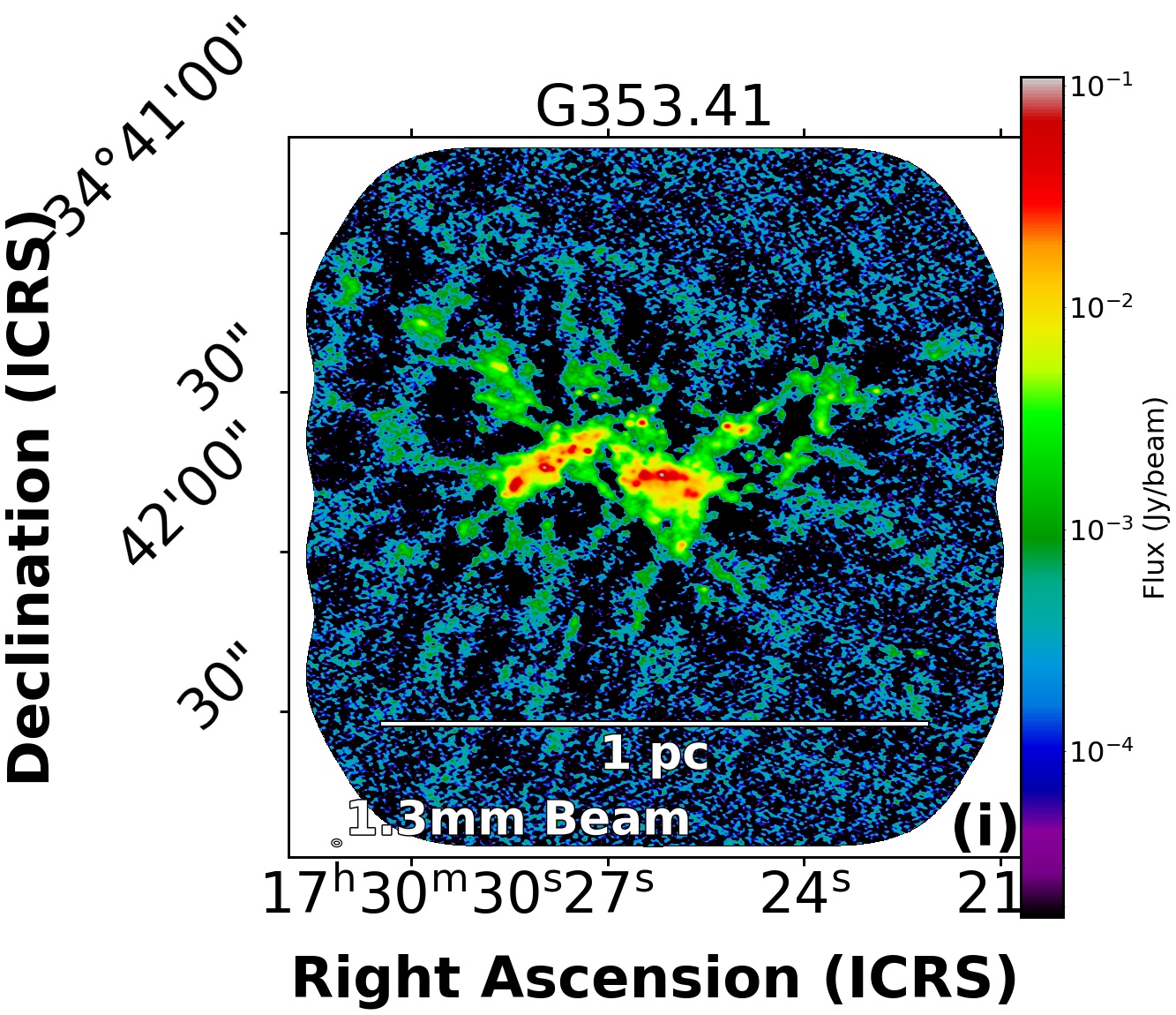
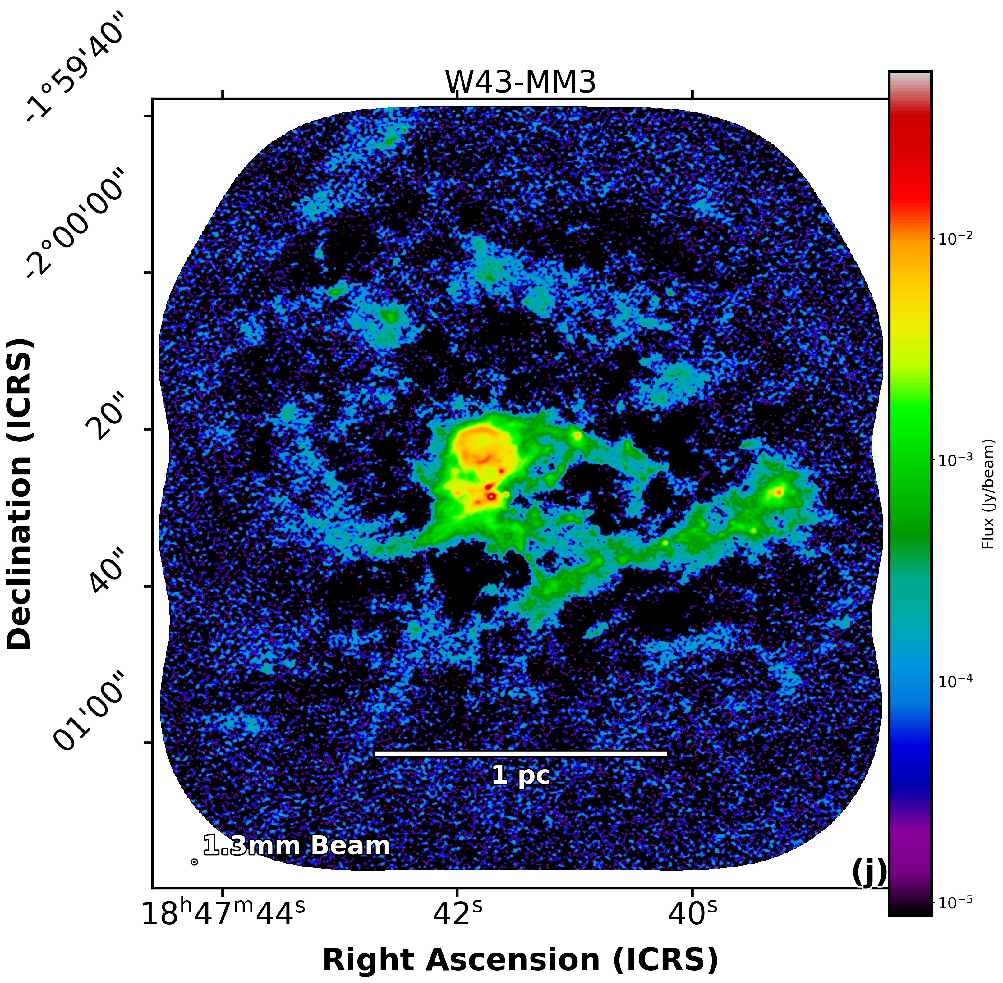
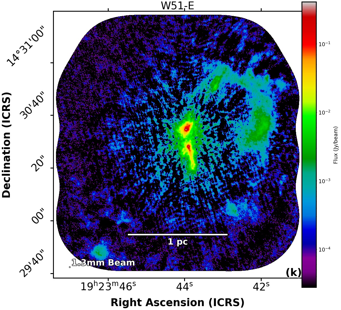
Figure 2: (Continued) 1.3 mm continuum ALMA 12 m array images of the Intermediate clouds: G351.77 (in g), G008.67 (in h), G353.41 (in i), W43-MM3 (in j), and W51-e (in k).

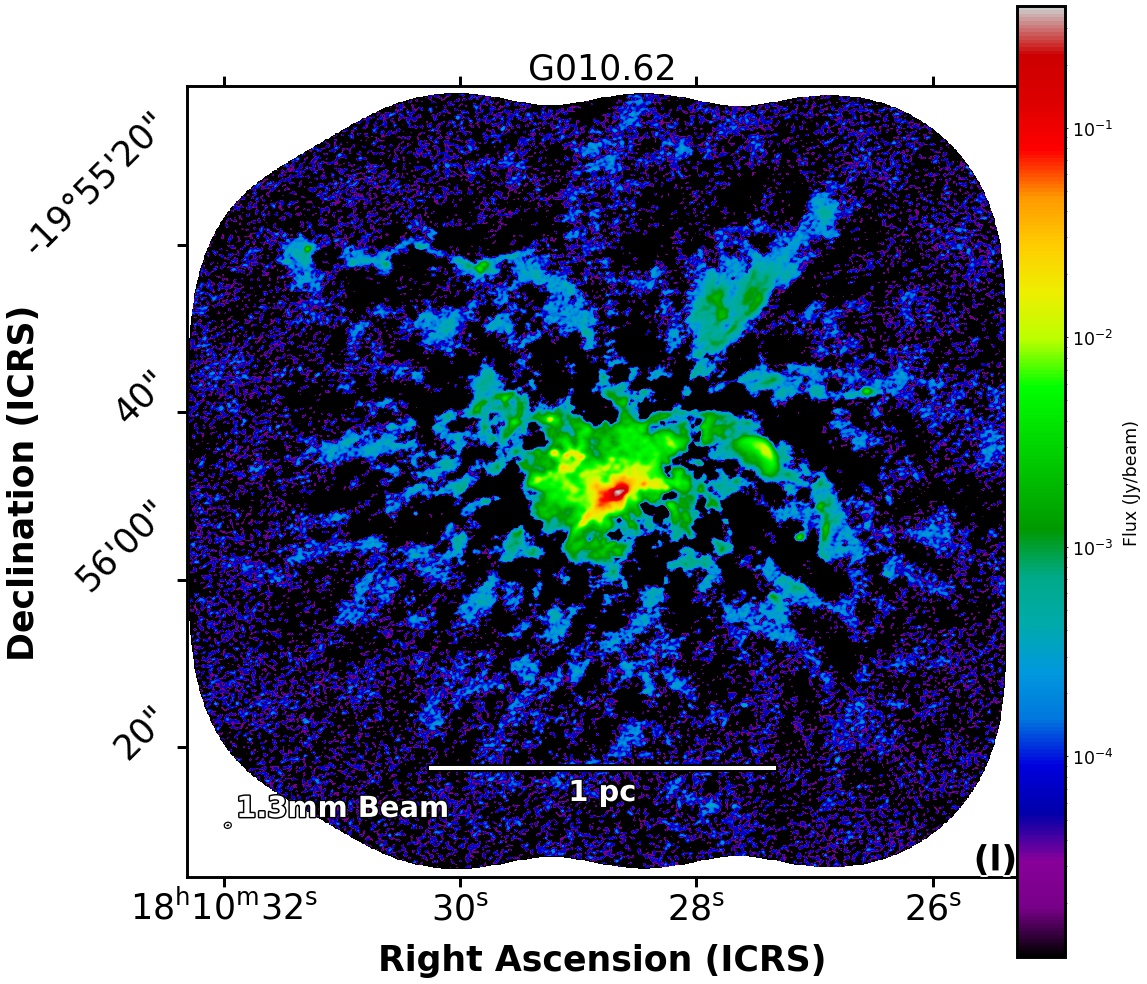
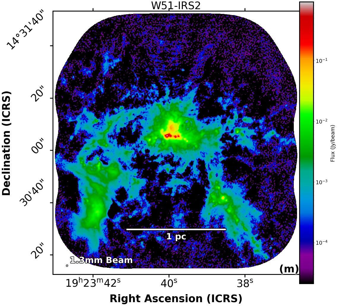
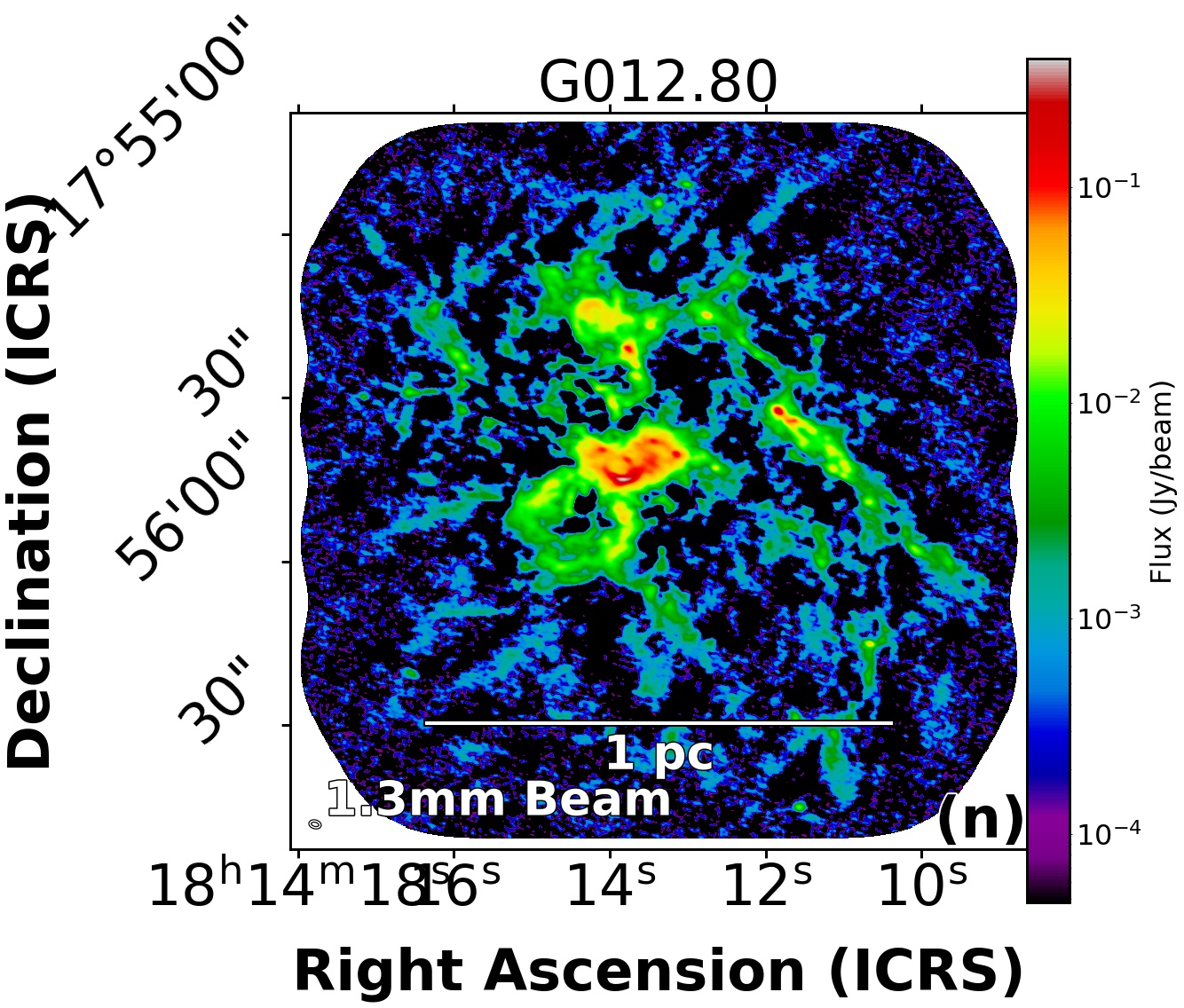
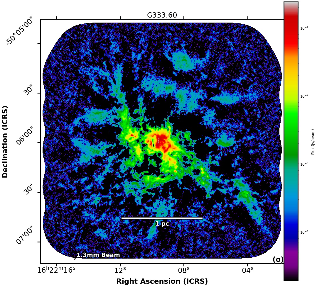
Figure 2: (Continued) 1.3 mm continuum ALMA 12 m array images of the Evolved clouds: G010.62 (in l), W51-IRS2 (in m), G012.80 (in n), and G333.60 (in o).

3.2 ALMA-IMF data set

The ALMA-IMF Large Program was observed from October 2017 to August 2018 with a total observation time of 69 hours and 172 hours with the 12 m and 7 m (ACA) arrays, respectively, and 595 hours with the Total Power Array. In this paper, we concentrate on the 1.3 mm and 3 mm mosaics done with the 12 m array (outlines are shown in Fig. 1), for the protocluster clouds of Table 1. Table 2 shows a summary of the imaged fields of view, angular resolutions, and sensitivities of the 12 m array continuum images at 1.3 mm and 3 mm. Table 4 lists the imaged 1.3 mm and 3 mm areas, which cover the whole extent of the protocluster clouds and their surroundings, respectively. The 1.3 mm areas were defined to systematically cover a 1 pc $\times$ 1 pc area around the targeted ATLASGAL clumps of Table 1, with larger areas for W43 and W51 clumps. The 3 mm areas aim to cover the filaments converging toward the ATLASGAL clumps (see Fig. 1). On average, these 15 massive protoclusters cover $\sim$3.5$\pm{2.0}\leavevmode\nobreak\ \mbox{pc}^{2}$ each, and sum up to $\sim$53$\leavevmode\nobreak\ \mbox{pc}^{2}$ (see Table 4).

The ALMA-IMF consortium built a pipeline that allows a homogeneous, repeatable, and high-quality reduction of its data set, starting with the 12 m array continuum mosaics (Ginsburg et al. in press.). Two sets of continuum images have been produced for each protocluster cloud and band. The first set of continuum images, called bsens, are derived using all observed spectral channels of the ALMA band 6 (1.3 mm or 228.965 GHz with a spectral index of $\alpha=3.5$) or band 3 (3 mm or 100.713 GHz with $\alpha=3.5$), summing up to 3.7 GHz and 2.9 GHz, respectively. The second set, constituting the cleanest continuum images, is built using only the line-free channels (see Ginsburg et al. in press., their Figs. 3–4). The bsens continuum images are up to two times more sensitive than the cleanest maps (see Table 2) but their continuum emission is contaminated by line emission. The 1.3 mm bsens images allow the detection of point-like cores down to the $3\,\sigma$ sensitivity level of $0.09\leavevmode\nobreak\ \mbox{$M_{\odot}$}$ to $0.5\leavevmode\nobreak\ \mbox{$M_{\odot}$}$, with a median of $\sim$0.18  $M_{\odot}$, corresponding to a point-source sensitivity of $\sim$7$\times 10^{22}$ cm^-2 in column density. Figure 2 presents the 1.3 mm images of the 15 ALMA-IMF clouds obtained from the 12 m array bsens data set of the ALMA-IMF Large Program. The 12 m array bsens and cleanest continuum images at 1.3 mm and 3 mm are provided to the community, along with the present paper and Paper II. The ALMA-IMF data processing pipelines and analysis are made public as described in Ginsburg et al. (in press.). The code is available on the github repository, https://github.com/ALMA-IMF/reduction, and ongoing work and data release updates can be found there and on the ALMA-IMF website (https://almaimf.com).

The angular resolutions achieved by the 12 m array ALMA continuum images at 1.3 mm and 3 mm, using the Briggs robust parameter robust=0, are within 30% of those requested, with the exception of a couple of outliers at 3 mm (see Table 2 of Ginsburg et al. in press.). Taking the distances of the ALMA-IMF clouds from Table 1, we computed the linear resolutions of the 1.3 mm and 3 mm bsens images. Listed in Table 5, the 1.3 mm spatial resolution ranges from 1 350 au to 2 690 au, with a median value and standard deviation of $2\,100\pm{400}$ au. As for the 3 mm images, they have on average a slightly better spatial resolution of $1\,800\pm{500}$ au. The dynamic range in angular scales (i.e., $DR=\theta_{\rm LAS}/\theta_{\rm beam}$, where $\theta_{\rm LAS}$ is the largest angular scale) ranges from $DR=6$ to 14 at 1.3 mm and $DR=7$ to 34 at 3 mm. The largest angular scale, also called maximum recoverable scale, spans ranges of $4.6\arcsec-6.6\arcsec$ at 1.3 mm and $4.8\arcsec-11\arcsec$ at 3 mm (see Table 2). They correspond to linear scales with mean values and $1\,\sigma$ dispersions of $\sim$0.1 pc and $\pm 0.03$ pc at 1.3 mm and $\sim$0.16 pc and $\pm 0.05$ pc at 3 mm, respectively, with maximum variation factors of $2.7-2.8$. The ratio of the 3 mm to 1.3 mm largest angular scales has a mean value of 1.7, close to the inverse ratio of the observed frequencies.

The line data cubes were processed within the framework of the ALMA-IMF data pipeline. The different 12 m array configurations were combined following the same procedure as for the continuum data, but cleaning and imaging is adapted to the line data cubes. They however first need to be corrected for the system temperature and the spectral data normalization (see also Sect.  2 of Ginsburg et al. in press.). The ALMA-IMF data were indeed affected by a systematic error in the spectral data normalization and returned to the Joint ALMA Observatory (JAO) for further processing in November 2020. Any data downloaded from the archive before this time are therefore affected by these issues. When processing is complete, line data cubes will be used to discuss the ionized component of the ALMA-IMF clouds, the cloud kinematics, outflows, and chemical enrichment. The sensitivities measured in the preliminary data cubes used here are $1\,\sigma=0.6-1$ K at 1.3 mm and $1\,\sigma=1.4-3.0$ K at 3 mm with a $1\leavevmode\nobreak\ \mbox{km\leavevmode\nobreak\ s${}^{-1}$}$ resolution.

As shown in Ginsburg et al. (in press.), the products combining ALMA 12 m array data with 7 m array data are of inconsistent quality across the ALMA-IMF sample. For several of the target fields, incorporating the 7 m array data resulted in increased noise levels and/or imaging artifacts. The increased noise levels is particularly problematic for source extraction on the $\sim$2 100 au scales. The 7 m array data are therefore not used for the present analysis.

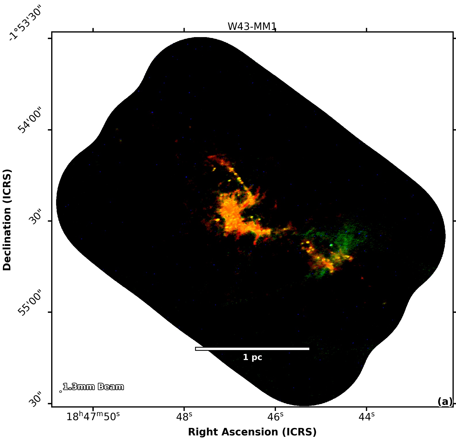
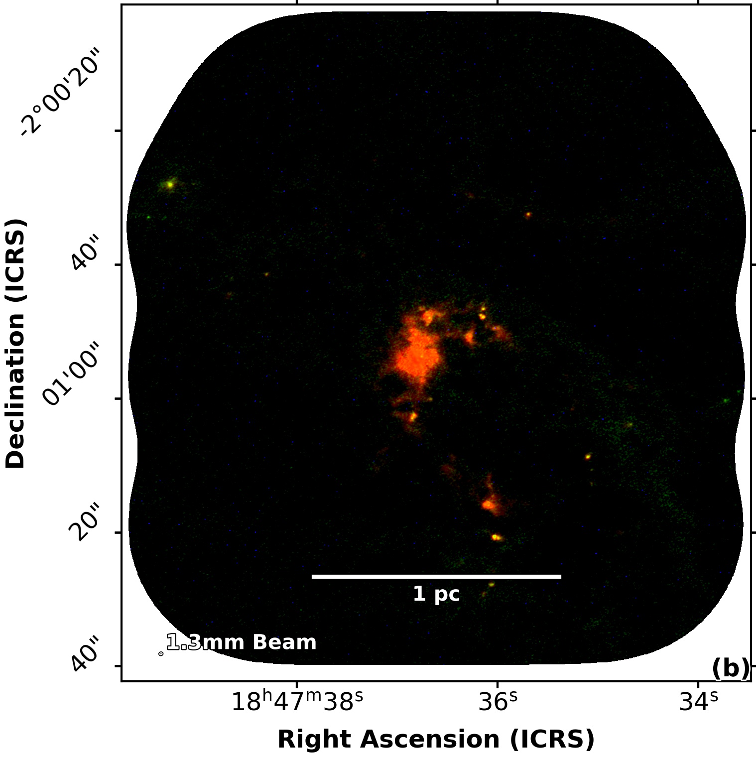
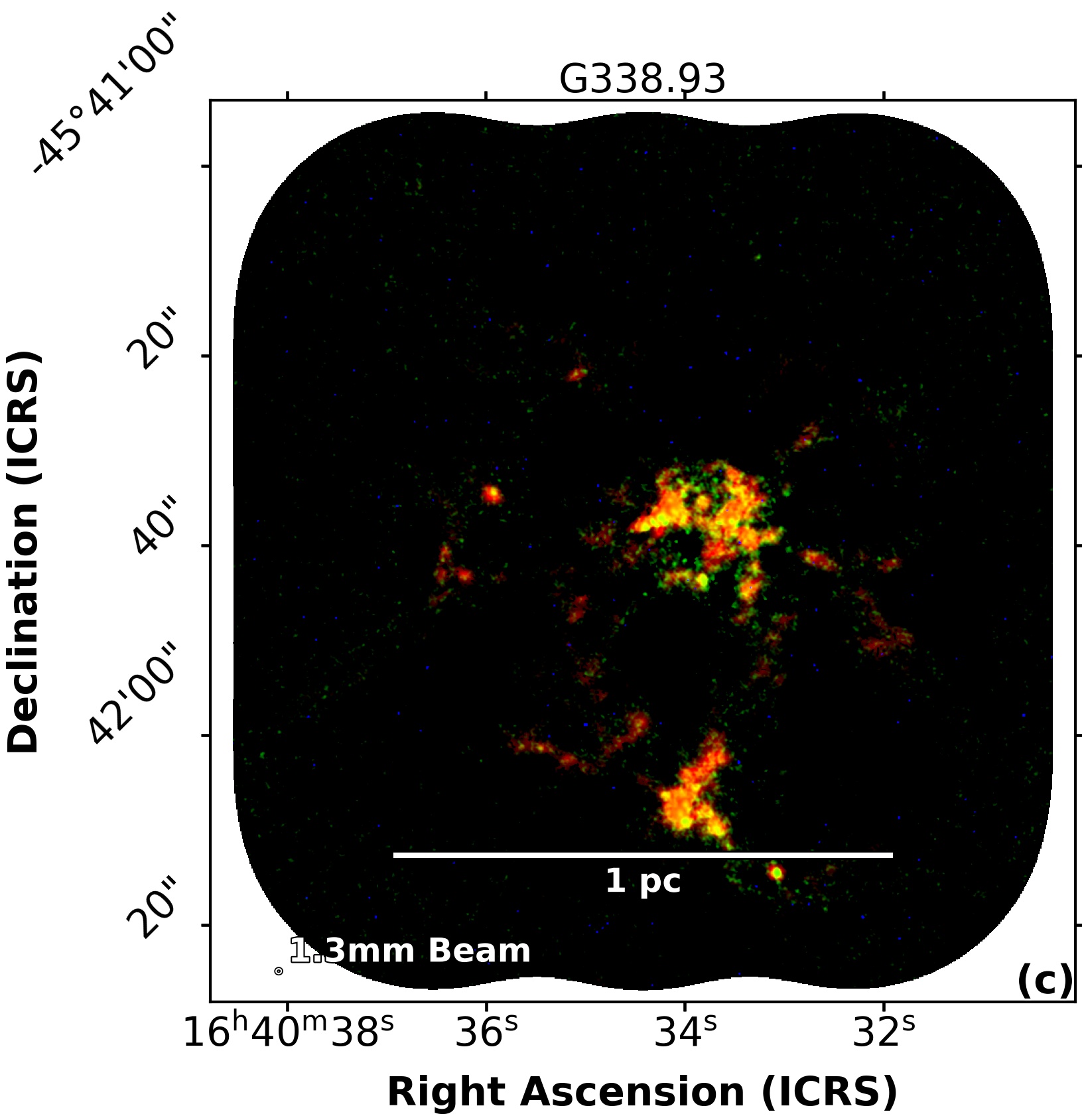
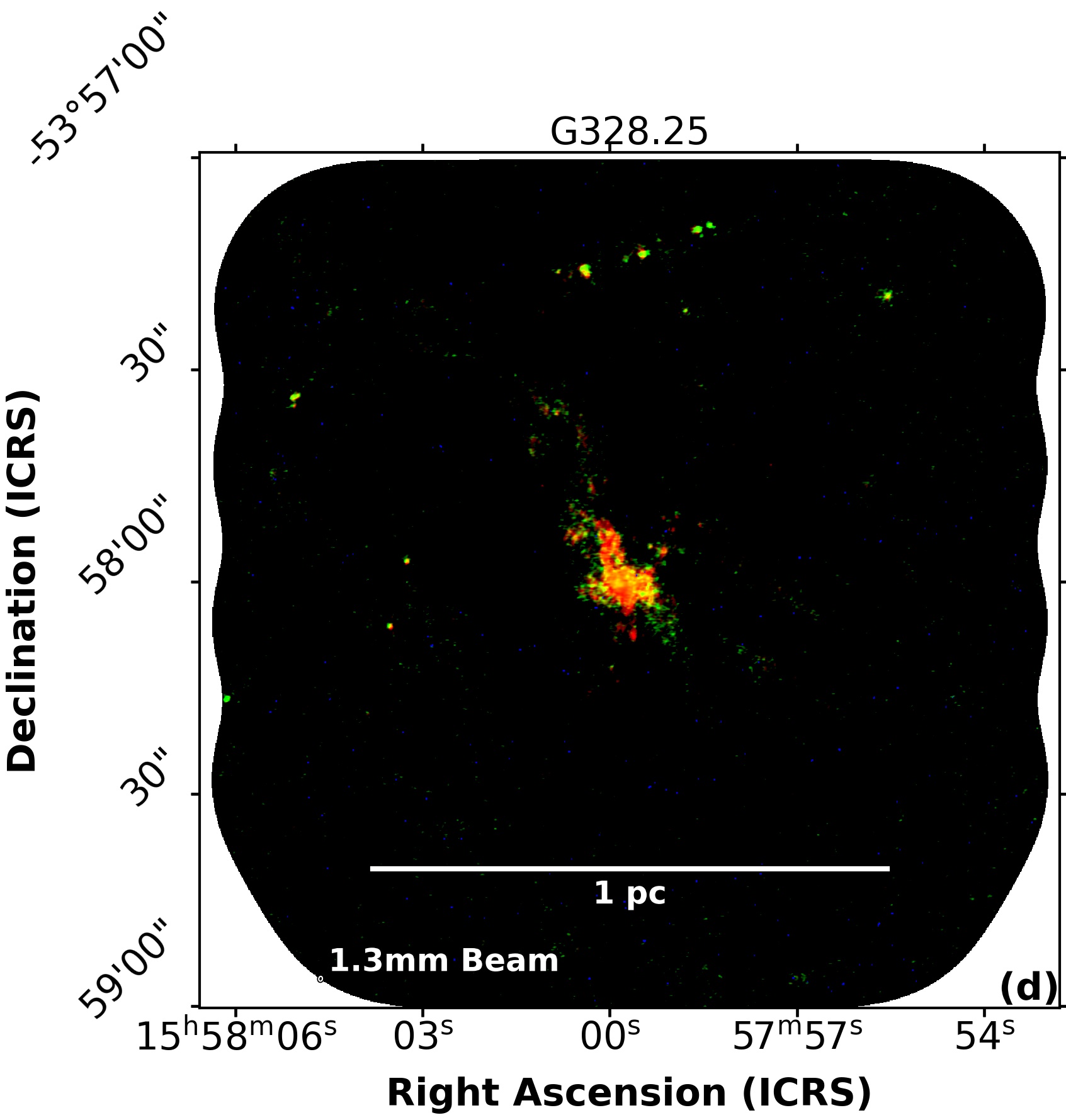
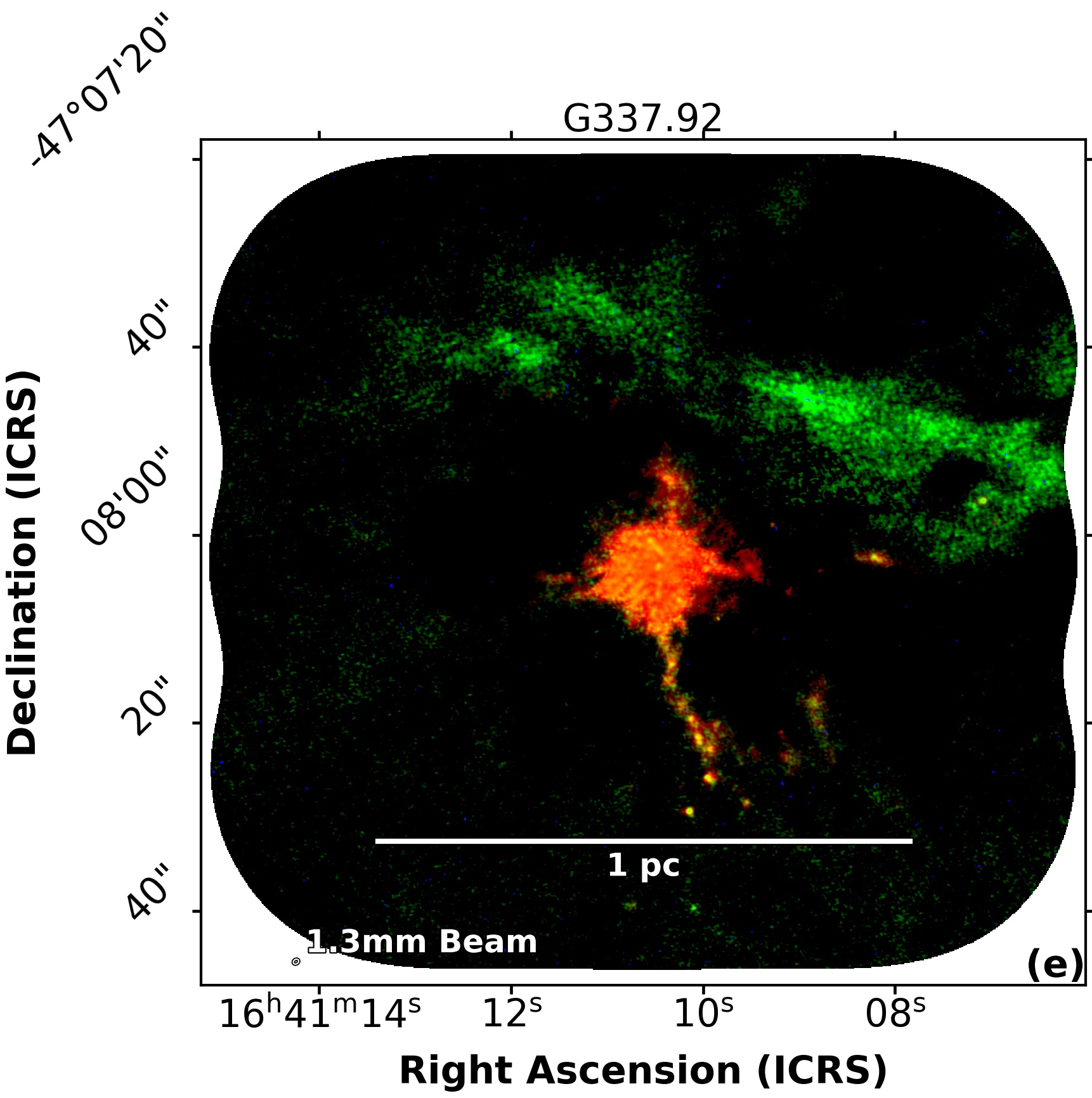
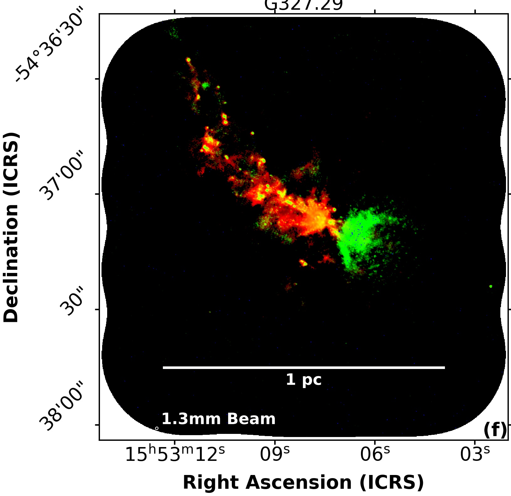
Figure 3: Three-color ALMA 12 m array images of the Young clouds: W43-MM1 (in a), W43-MM2 (in b), G338.93 (in c), G328.25 (in d), G337.92 (in e), and G327.29 (in f), plotted at the same physical scale. Red and green display the continuum images at 1.3 mm and 3 mm, respectively, with the green color for the longer, 3 mm, wavelength because the 3 mm emission is partly associated with hot ionized gas. Blue corresponds to the free-free emission at the frequency of the H$41\alpha$ recombination line. Thermal dust emission of filaments and cores is shown in orange shades, while diffuse green features locate weak free-free emission from faint H ii regions in e and f.

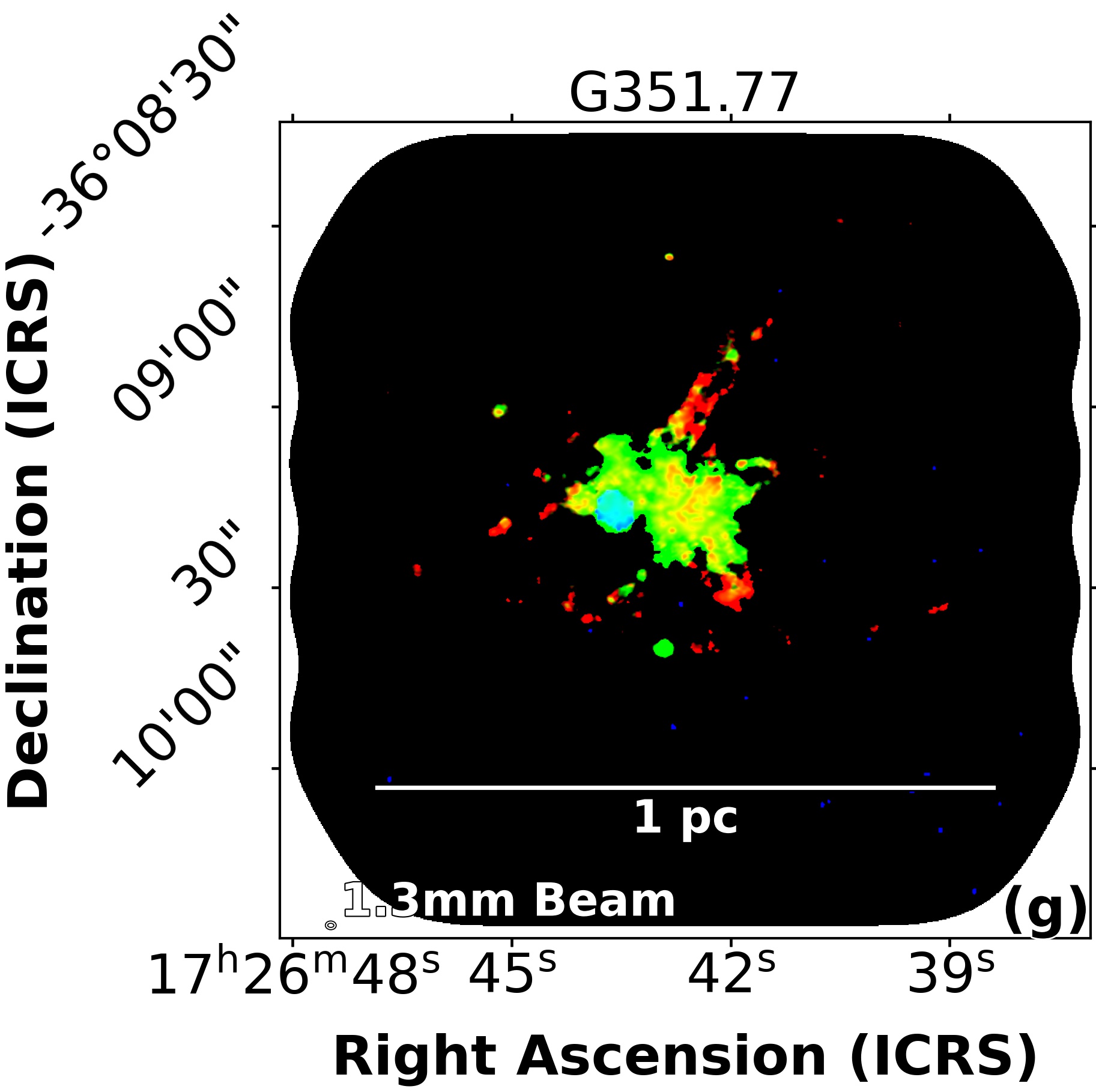
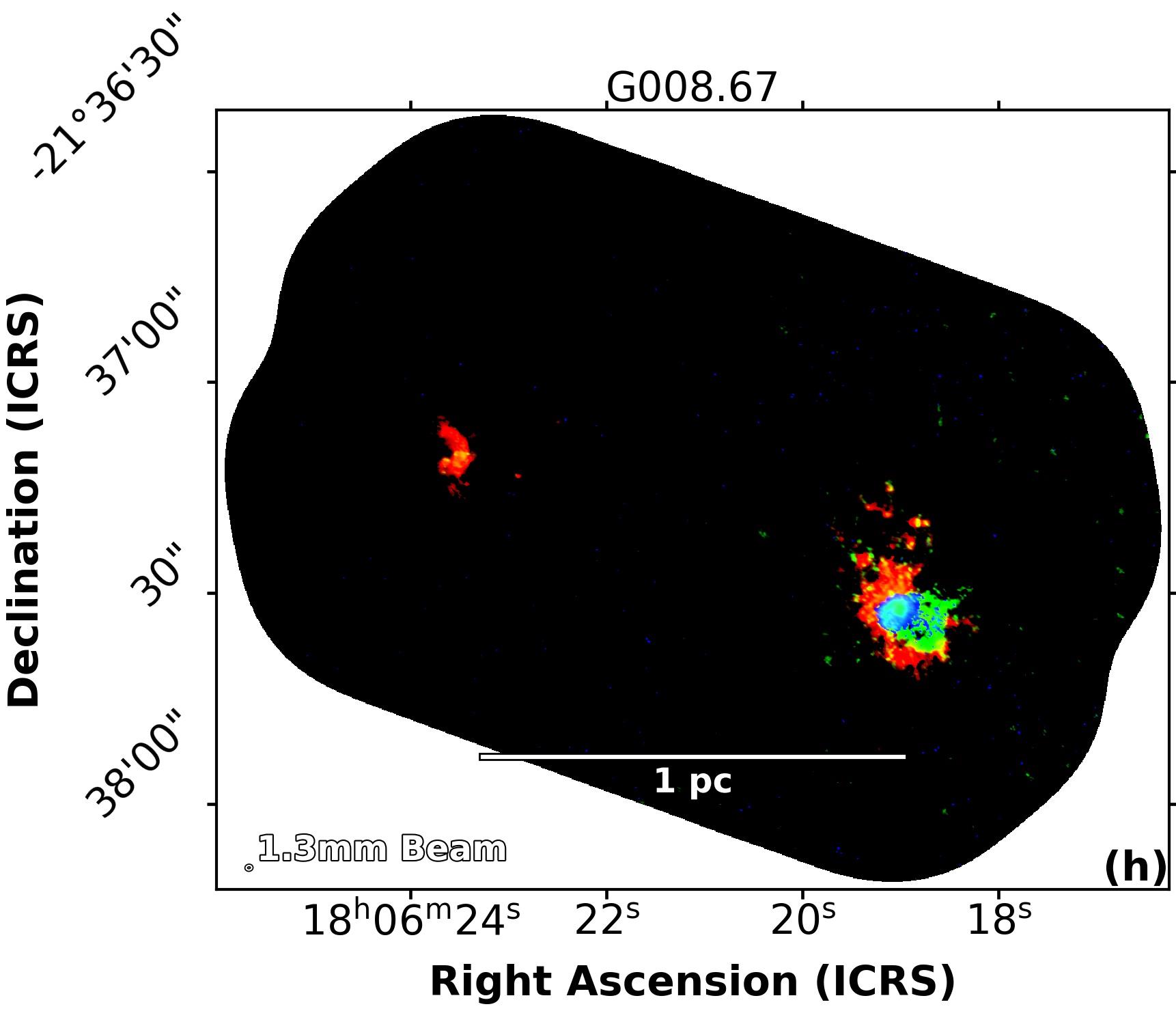
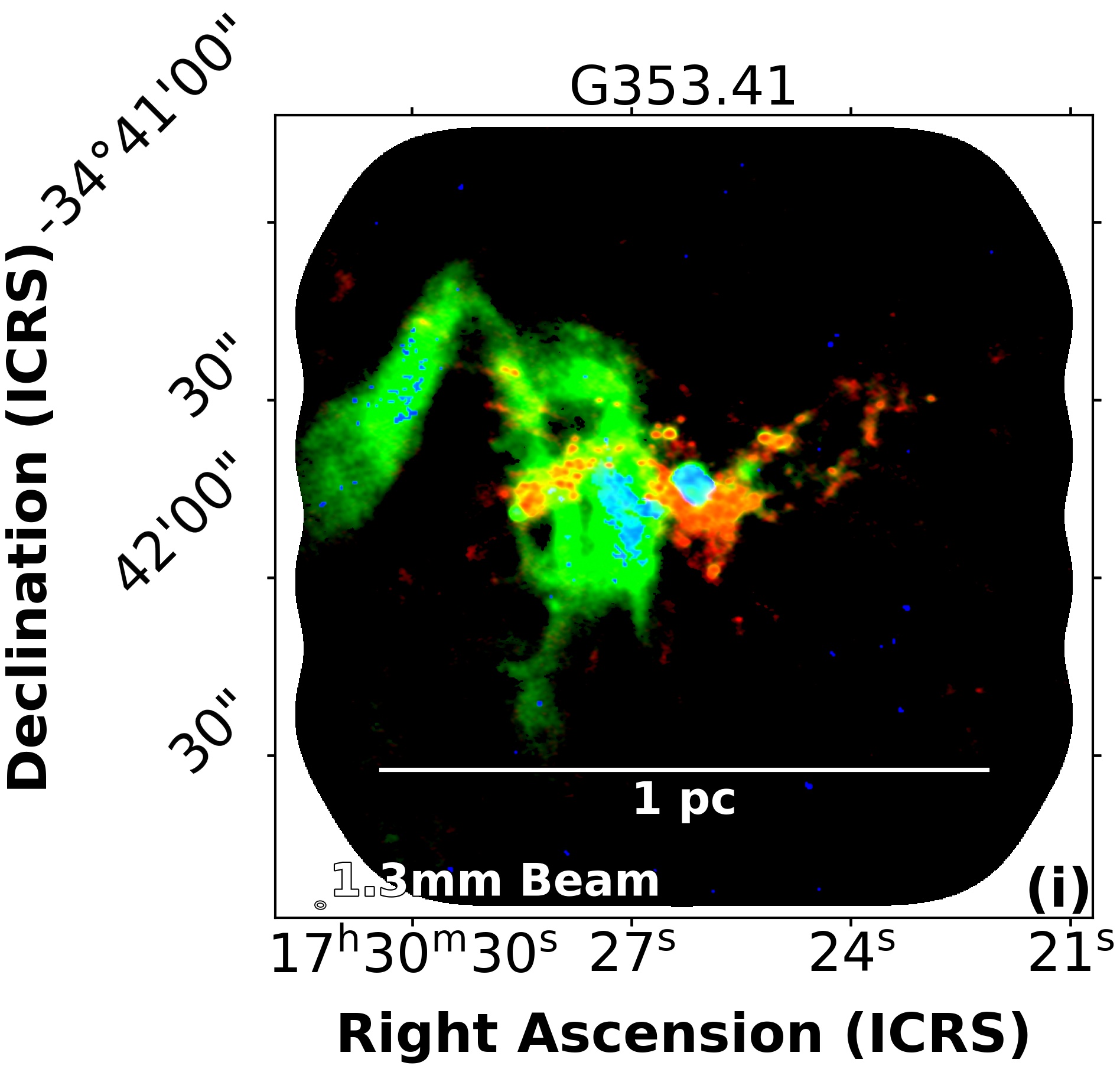
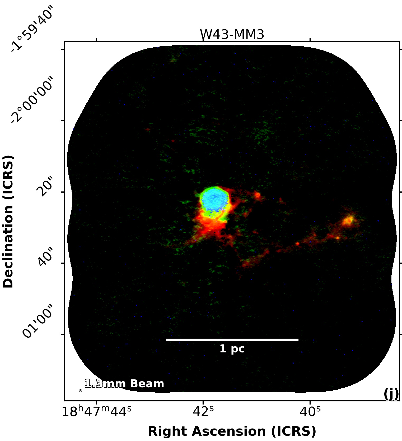
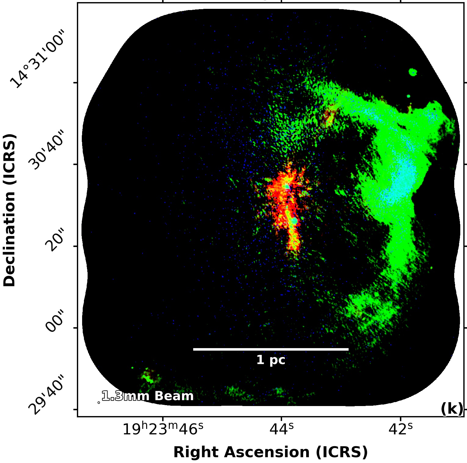
Figure 3: (Continued) Three-color ALMA 12 m array images of the Intermediate clouds: G351.77 (in g), G008.67 (in h), G353.41 (in i), W43-MM3 (in j), and W51-e (in k). The coincidence of blue and green emission locates six HC or UCH ii region bubbles (in g–k) and diffuse arc-like emission of compact to extended H ii regions (in i and k).

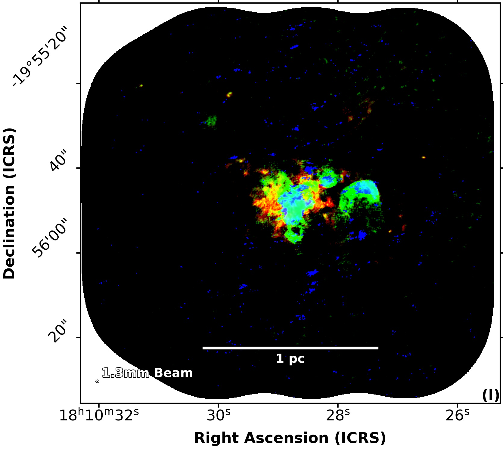
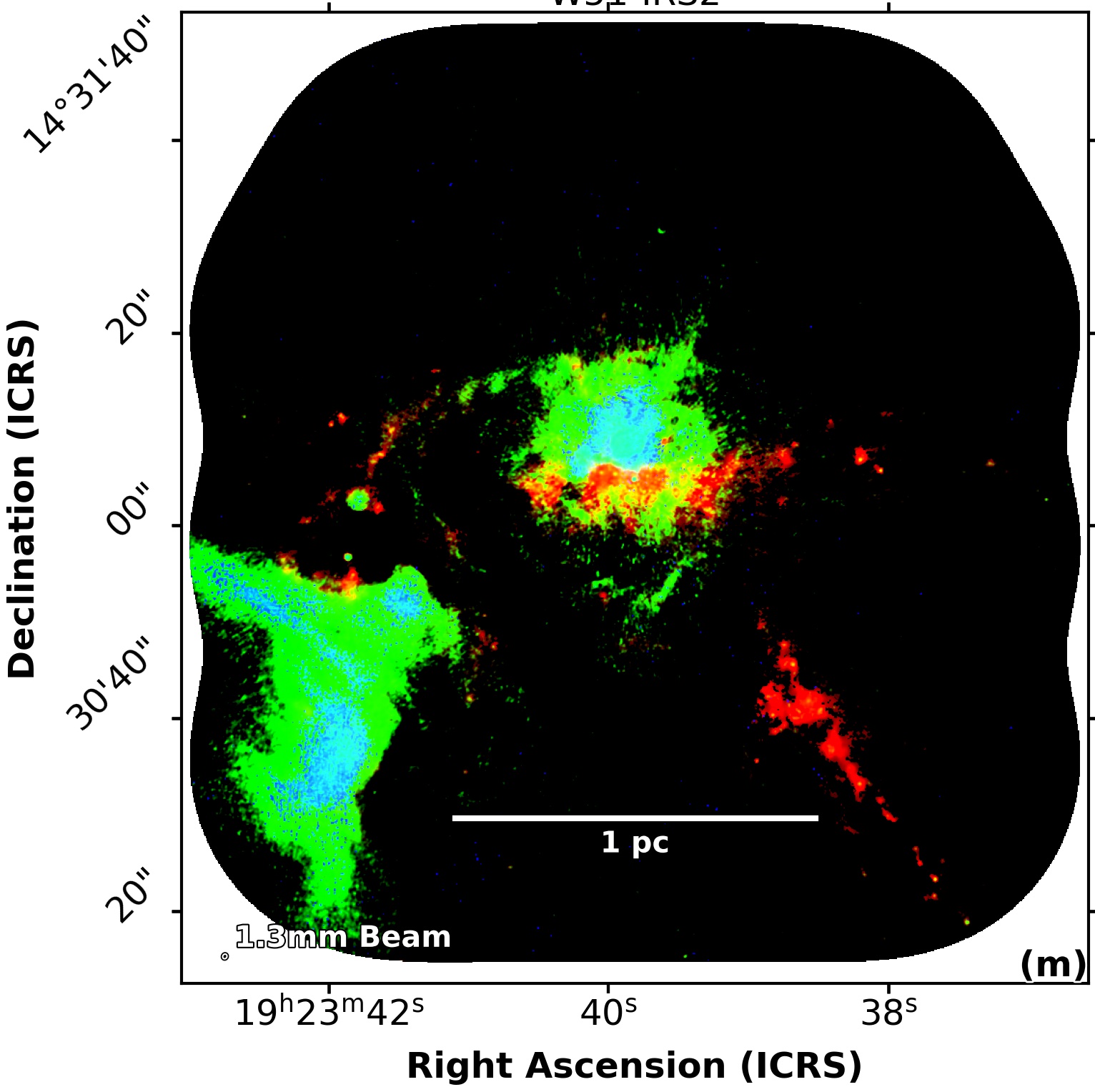
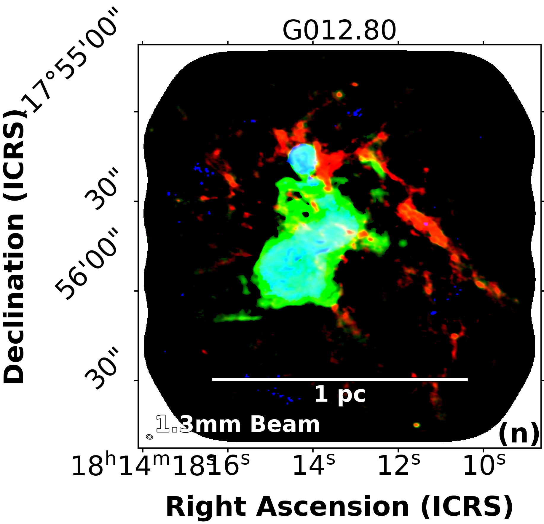
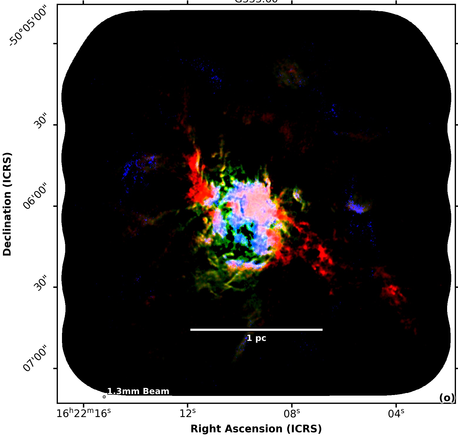
Figure 3: (Continued) Three-color ALMA 12 m array images of the Evolved clouds: G010.62 (in l), W51-IRS2 (in m), G012.80 (in n), and G333.60 (in o). There is an almost complete coincidence between the free-free emission at the H$41\alpha$ recombination line frequency (blue) and the 3 mm continuum (green), which is dominated in l–o by free-free emission. Red filamentary structures represent the few locations where thermal dust emission dominates the continuum millimeter emission.

4 First results and survey potential

We present here the continuum images and preliminary line data set used to refine the evolutionary stage classification of the ALMA-IMF protoclusters (see Sect. 4.1), to characterize their core content (see Sect. 4.2) and the gas concentration from cloud to cores (see Sect. 4.3), and to discuss the potential of ALMA-IMF data to constrain the gas kinematics and molecular complexity of clouds (see Sects. 4.4–4.5).

Table 4 lists the main characteristics of the ALMA-IMF protocluster clouds, among which is their total cloud mass, $M^{\rm cloud}_{\rm 870\,\mu m}$, integrated over the ALMA-IMF 1.3 mm image coverage. This mass is computed from the $870\,\mu$m flux of the clouds, $S^{\rm cloud}_{\rm 870\,\mu m}$, using Section 2.2. Given that the temperatures of the brightest ATLASGAL sources, as measured in NH₃, vary (Wienen et al. 2012, 2015; see also Fig. 7 of Csengeri et al. 2017), we assumed $\mbox{$T_{\rm dust}$}=20$ K, 25 K and 30 K, for the Young, Intermediate, and Evolved clouds (as defined in Sect. 4.1), respectively. Assuming a single $\mbox{$T_{\rm dust}$}=20$ K temperature would increase the mass of Intermediate and Evolved clouds by 1.3 and 1.75, respectively.

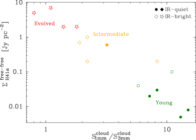
Figure 4: Evolutionary sequence of the ALMA-IMF protoclusters, assuming that free-free emission increases over time. The 1.3 mm-to-3 mm flux ratios decrease when the free-free emission dominates the thermal dust emission at 3 mm. The provisional evolutionary stage of IR-quiet and IR-bright protoclusters is indicated by filled and empty square markers, respectively. Their revised evolutionary stage, from Young, to Intermediate, to Evolved, are shown by green, orange, and red markers, respectively.

4.1 Evolutionary stage of the ALMA-IMF protoclusters

We have improved the initial evolutionary stage classification of the 15 protoclusters listed in Table 1, separating them between Young, Intermediate, and Evolved protoclusters. Determining the evolutionary stage of a $\mbox{pc}^{2}$-size cloud is nontrivial because its structures are expected to form continuously, concentrate, form stars, heat, be partly ionized, and finally disperse. To this end, we utilize two criteria: the 1.3 mm-to-3 mm flux ratio and the free-free emission at the frequency of the H41$\alpha$ recombination line. They both hinge on the assumption that as high-mass, gas-dominated star-forming protoclusters evolve, they will host more and more H ii regions. Thus, the free-free emission is assumed to increase over time as their H ii bubbles expand and the number of H ii sources increases. We summarize in Fig. 4 the evolutionary sequence of the 15 ALMA-IMF protoclusters that is defined using these two criteria and from a visual inspection of Fig. 3.

We first computed the 1.3 mm-to-3 mm flux ratios of ALMA-IMF clouds using their 1.3 mm and 3 mm 12 m array bsens images (see Fig. 2 and Fig. 1 of Ginsburg et al. in press.). For more evolved clouds, the free-free emission of compact and developed H ii regions (CH ii $\rightarrow$ $\rm H\mbox{\sc\leavevmode\nobreak\ ii}$) can dominate at 3 mm, while thermal dust emission would be the major component of the 1.3 mm emission (e.g., Ginsburg et al. 2020). The 1.3 mm to 3 mm flux ratio is therefore expected to decrease over time from its value associated with thermal dust emission, to 0.9 for a flat spectral energy distribution ($\alpha(\nu)=-0.1$, e.g., Keto et al. 2008). The 1.3 mm ($\nu_{\textrm{B6}}=229.0$ GHz; see Table D1 in Ginsburg et al. in press.) to 3 mm ($\nu_{\textrm{B3}}=100.78$ GHz) flux ratio of thermal dust emission from clouds at $\mbox{$T_{\rm dust}$}=20-30$ K (see Table 1) is expected to be on the order of 20, assuming optically thin emission and with a dust emissivity index of $\beta=1.8$, well suited for clouds (Planck Collaboration et al. 2011). We integrated the 1.3 mm and 3 mm fluxes over the common 1.3 mm imaged area (see Table 4) and computed the ratios of integrated fluxes, $S^{\rm cloud}_{\rm 1.3\,mm}/S^{\rm cloud}_{\rm 3\,mm}$. In Table 4, the global ratios of the 15 clouds vary from 0.8 to 15, with median values of $\sim$8 and $\sim$2 and $1\,\sigma$ dispersions of $\pm{4}$ and $\pm{3}$ for the IR-quiet and IR-bright cloud populations, respectively.

The evolutionary status derived from the 1.3 mm-to-3 mm flux ratio is consistent with that derived from the 1.3 mm-to-3 mm spectral index measured both between and within the observed bands (Ginsburg et al. in press.). The 1.3 mm-to-3 mm flux ratio suggests that, except for three clouds, the IR-quiet/IR-bright classification of protoclusters using their mid-IR flux remains valid. Among the exceptions, the IR-quiet protocluster cloud G008.67 has a low 1.3 mm-to-3 mm flux ratio suggesting that it does not qualify as being Young. Conversely, the IR-bright protocluster clouds G327.29, G337.29, and G351.77 have high ratios that conflict with their previous classification as evolved objects. This tendency is confirmed in Fig. 3, which presents the three-color ALMA images of the whole ALMA-IMF sample, using the 1.3 mm and 3 mm continuum emission for two of the three color images (red and green). The ALMA imaging indeed separates the cold cloud at the centers of both G327.29 and G337.92 from the developed H ii regions lying at their peripheries (west of G327.29 and north of G337.92). A scaling by the theoretical ratio of thermal dust emission at 20 K shows that thermal dust emission dominates over the whole extent of six protocluster clouds, which we classify as Young (see Figs. 3a–e). Their mean flux ratio, $S^{\rm cloud}_{\rm 1.3\,mm}/S^{\rm cloud}_{\rm 3\,mm}\simeq 11$ with a $1\,\sigma$ dispersion of $\pm{3}$, is smaller than the theoretical one, $20$. Here diffuse free-free emission is sporadically present at the peripheries of the targeted clouds (as in Figs. 3a, e–f) and the extended emission is on average filtered to scales 1.7 times smaller in the 1.3 mm images than in the 3 mm images (see Sect. 3.2).

[c]

Table 5: Gas mass distribution within ALMA-IMF protoclusters, from parsec-size clouds to structures with typical sizes of 0.1 pc and finally to 2100 au cores.

Protocluster	Spatial	$S^{\rm recovered}_{\rm 1.3\,mm}$	$M^{\rm recovered}_{\rm 1.3\,mm}$	Number of		$M^{\rm cores}_{\rm 1.3\,mm}$	$M^{\rm recovered}_{\rm 1.3\,mm}$	$M^{\rm cores}_{\rm 1.3\,mm}$	$M^{\rm cores}_{\rm 1.3\,mm}$
cloud name	resolution	within $A_{\rm 1.3\,mm}$	within $A_{\rm 1.3\,mm}$	extracted	cores3	within $A_{\rm 1.3\,mm}$	$/M^{\rm cloud}_{\rm 870\,\mu m}$	$/M^{\rm recovered}_{\rm 1.3\,mm}$	$/M^{\rm cloud}_{\rm 870\,\mu m}$
	[au]	[Jy]1	[$M_{\odot}$]2	sources	[#, %]	[$M_{\odot}$]	[%]4	[%]	[%]
(1)	(2)	(3)	(4)	(5)	(6)	(7)	(8)	(9)	(10)
W43-MM1	2 430	10.4	6 200	57	56 (98%)	872	46%	14%	6.5%
W43-MM2	2 540	2.9	1 700	43	38 (88%)	294	15%	17%	2.5%
G338.93	2 080	3.0	890	51	51 (100%)	509	13%	57%	7.2%
G328.25	1 350	1.4	180	18	18 (100%)	69	7%	38%	2.7%
G337.92	1 460	5.1	720	38	37 (97%)	160	28%	22%	6.3%
G327.29	1 650	$16.9-16.4$	2 010	47	41 (87%)	497	41%	25%	9.7%
G351.77	1 540	$10.3-10.2$	800	28	26 (93%)	277	32%	35%	11%
G008.67	2 250	$3.7-2.2$	500	22	21 (95%)	126	16%	25%	4.1%
W43-MM3	2 690	$2.5-1.9$	1 100	35	34 (97%)	164	21%	15%	3.1%
W51-E	1 640	$30.1-27.6$	16 000	58	39 (67%)	743	48%	5%	2.3%
G353.41	1 590	$6.6-5.4$	420	62	59 (95%)	132	17%	31%	5.3%
G010.62	2 310	$8.7-3.1$	1 500	61	47 (77%)	181	22%	12%	2.7%
W51-IRS2	2 560	$22.8-16.9$	9 600	117	96 (82%)	825	47%	9%	4.0%
G012.80	2 110	$22.3-7.7$	860	82	65 (79%)	277	18%	32%	6.0%
G333.60	2 330	$34.8-6.8$	2 300	118	66 (56%)	461	22%	20%	3.8%

• Flux recovered by the ALMA 12 m array at 1.3 mm and integrated over the 1.3 mm imaged area. In the case of Intermediate and Evolved protocluster clouds and G327.29, a second value, corrected for free-free contamination, is given by ignoring the 1.3 mm fluxes in areas where the free-free emission dominates (as indicated by the H41$\alpha$ image).

• Mass recovered by the ALMA 12 m array computed from the total 1.3 mm fluxes corrected for free-free contamination (Col. 3, right value) and using Section 4.2 with $\kappa_{\rm 1.3\,mm}=\rm 0.01\leavevmode\nobreak\ cm^{2}\,g^{-1}$ and $\mbox{$T_{\rm dust}$}=20$ K.

• Cores are sources extracted at 1.3 mm (Col. 5), whose emission consists of thermal dust emission. The sources of Col. 5, which are not included in Col. 6 are candidate ionization peaks detected through their free-free emission.

• Assuming the same temperature for all type of clouds when measuring their total cloud mass, the gas mass concentration from 1 pc to 0.1 pc cloud structures would be reduced by factors of 1.3 and 1.75 for Intermediate and Evolved clouds, respectively.

Owing to the uncertainties from the overall 1.3 mm-to-3 mm flux ratios, we introduced a second criterion based on estimates of the free-free continuum emission (shown in blue in the three-color images, Fig. 3) using cubes of the H41$\alpha$ hydrogen recombination line. For each ALMA-IMF cloud, we created an H41$\alpha$ image by integrating its spectral cube over the velocity extent of the H41$\alpha$ line. The cloud H41$\alpha$ emission, $S_{\mathrm{H41\alpha}}^{\mathrm{>5\,\sigma}}$, is derived from this image clipped at $5\,\sigma$ and integrated over the cloud area. Assuming local thermodynamical equilibrium, the free-free emission of each ALMA-IMF cloud, $S^{\rm free-free}_{\rm H41\alpha}$, is then computed following

$$S^{\rm free-free}_{\rm H41\alpha}=1.432\times 10^{-4}\times S_{\mathrm{H41\alpha}}^{\mathrm{>5\sigma}}\times\nu_{0}^{-1.1}\,T_{e}^{1.15}\,(1+N_{\mathrm{He}}/N_{\mathrm{H}})^{-1},$$ (2)

where $\nu_{0}=92.034$ GHz is the rest frequency of the H41$\alpha$ line and we assume an electron temperature of $T_{e}=8000$ K and a relative abundance of helium to hydrogen of $N_{\mathrm{He}}/N_{\mathrm{H}}=0.08$. We finally converted the free-free emission, $S^{\rm free-free}_{\rm H41\alpha}$, to a flux surface density, $\Sigma^{\rm free-free}_{\rm H41\alpha}=S^{\rm free-free}_{\rm H41\alpha}/A_{\rm 1.3\,mm}$, in Jy pc^-2. Table 4 lists $\Sigma^{\rm free-free}_{\rm H41\alpha}$ values, which are a good proxy for the average amount of ionized gas in ALMA-IMF clouds. These averaged surface densities of free-free emission have the advantage of being independent of the area of the imaged cloud and, here, $A_{\rm 1.3\,mm}$ ranges from 1.3 pc² to 8.4 pc² (see Table 4). Because we designed the survey to have matched sensitivity across all clouds, for $\lesssim$0.16 pc emissions at the H41$\alpha$ frequency (see Sect. 3.2), and because most of the free-free emission detected in ALMA 12 m array images arise from H ii regions of small sizes (see Fig. 3), $\Sigma^{\rm free-free}_{\rm H41\alpha}$ does not have a strong distance dependence. The values given in Table 4 can therefore be compared without strong bias from one cloud to another.

The extrema of the present classification are the most informative as they are more robust. Considering the IR-bright sources, we observe that G333.60, G010.62, W51-IRS2, and G012.80 all have strong flux surface densities, $\Sigma^{\rm free-free}_{\rm H41\alpha}\simeq 4\leavevmode\nobreak\ \rm Jy\,pc^{-2}$ with a $1\,\sigma$ dispersion of $\pm 2\leavevmode\nobreak\ \rm Jy\,pc^{-2}$, as well as complex and extended H$41\alpha$ emission, positionally correlated 3 mm and H$41\alpha$ emission, and low 1.3 mm-to-3 mm flux ratios, $S^{\rm cloud}_{\rm 1.3\,mm}/S^{\rm cloud}_{\rm 3\,mm}\simeq 1.3$ with a dispersion of $\pm{0.4}$. These features together are consistent with advanced H ii activity compared to the other sources in our sample. These four protoclusters are therefore classified as Evolved. Turning next to the IR-quiet sources in Csengeri et al. (2017), Young protoclusters are barely detected in H$41\alpha$, with flux surface densities of their free-free emission two orders of magnitude smaller than those measured for Evolved clouds, median $\Sigma^{\rm free-free}_{\rm H41\alpha}\simeq 0.05\rm\leavevmode\nobreak\ Jy\,pc^{-2}$ with a dispersion of $\pm 0.04\leavevmode\nobreak\ \rm Jy\,pc^{-2}$, and with no coherent structure detected (see Table 4 and Fig. 4).

In between these extrema, we identify the Intermediate protoclusters, which have properties consistent with different aspects of both the Young and Evolved categories described above. Namely, these protoclusters host both dense filamentary structures traced by their thermal dust emission and a couple of small, localized bubbles of ionized gas (see Fig. 3g–k). The latter are generally qualified as hyper-compact H ii (HC$\rm H\mbox{\sc\leavevmode\nobreak\ ii}$) regions when they develop in a dense, $\sim$10⁶ cm^-3, medium and their extent is smaller than 0.05 pc (Hoare et al. 2007). They become ultra-compact H ii (UC$\rm H\mbox{\sc\leavevmode\nobreak\ ii}$) when they are more extended and develop in a less dense medium, $\sim$0.1 pc and $\sim$10⁴ cm^-3 (e.g., Kurtz et al. 2000). These young H ii regions are traced by their free-free emission detected both in the 1.3 mm continuum emission band and by the H41$\alpha$ recombination line. G351.77, W43-MM3, W51-E, and G353.41 are four IR-bright protocluster clouds that present those characteristics (see Figs. 3g, i–k). In addition, the G008.67 protocluster cloud, whose IR-quiet classification was already questionable due to its low 1.3 mm-to-3 mm flux ratio, displays an UCH ii region, which qualifies it as Intermediate (see Fig. 3h). The flux surface densities of the free-free continuum emission of Intermediate protocluster clouds, median $\Sigma^{\rm free-free}_{\rm H41\alpha}=0.5\rm\leavevmode\nobreak\ Jy\,pc^{-2}$ with a $1\,\sigma$ dispersion of $\pm 0.3\leavevmode\nobreak\ \rm Jy\,pc^{-2}$, is about ten times lower than that of Evolved protocluster clouds and ten times higher than that of the Young ones (see Table 4).

We therefore have set up three groups of protocluster clouds according to their evolutionary stage. Six qualify as Young clouds, five as Intermediate, and four as Evolved (see Table 4). This classification is based on visual inspection of the distribution of free-free emission, continuum emission, and multiwavelength continuum ratios, and thus incorporates a wealth of observational information. We robustly distinguish protoclusters devoid of internal ionizing sources, those which harbor a couple of HCH ii or UCH ii regions, and protoclusters whose structure is intertwined with developed and bright H ii regions. Figure 4 displays a good correlation between the two quantitative criteria used here, suggesting that the variation in the spatial filtering within the cloud sample (see Sect. 3.2) has no significant impact on our classification.

As shown in Tables 1 and 4, the three classes of protoclusters span the same range of distances to the Sun, demonstrating that to first order no distance biases affect our classification. The Young and Intermediate protocluster clouds are however much smaller in size than the Evolved ones, their median values being $\sim$2.1 pc² and $\sim$2.6 pc² versus $\sim$4.8 pc². The total protocluster gas masses of the Young, Intermediate, and Evolved clouds have median values within a factor of two from each other: $\sim$$6\times 10^{3}\leavevmode\nobreak\ \mbox{$M_{\odot}$}$, $\sim$$3\times 10^{3}\leavevmode\nobreak\ \mbox{$M_{\odot}$}$, and $\sim$$9\times 10^{3}\leavevmode\nobreak\ \mbox{$M_{\odot}$}$, respectively.

4.2 Population of cores in the ALMA-IMF protoclusters

The star-formation activity of the ALMA-IMF massive clouds, and therefore the richness of the ALMA-IMF core database, can be assessed by the number of cores one can detect. In Paper III, Louvet et al. (in prep.) extracted sources from the cleanest continuum images (see definition in Sect. 3.2) and identified about 840 compact sources. Moreover, we showed that using both the bsens and cleanest images (see definitions in Sect. 3.2), the number of robust core detections could further increase by a factor of up to $\sim$2 (Pouteau et al. in prep.). Extracting these additional sources requires careful treatment of the line contamination to exclude emission peaks associated with line rather than continuum emission. The additional sources are predominantly lower-mass cores and the fluxes of common sources are consistent between the two approaches. One can also gain in source detections using images where the cirrus noise is reduced by the Multiscale non-Gaussian Segmentation (MnGSeg) technique (Robitaille et al. 2019). MnGSeg separates these cloud structures, which are incoherent from one scale to another and referred to as Gaussian, from the filaments and cores, which are coherent structures and are associated with star formation. Thus, the core database of the ALMA-IMF Large Program can potentially contain about $1\,500$ objects. To focus on cores that are real density peaks, Louvet et al. (in prep.) excluded millimeter sources that could correspond to free-free continuum peaks, that is, sources associated with inhomogeneities of H ii regions that develop in the ALMA-IMF protoclusters. This exclusion marginally reduced the number of cores by $\sim$5% in Young regions, $\sim$13% in Intermediate regions and reduced it further, by $\sim$27%, in Evolved clouds. Table 5 lists, for each of the ALMA-IMF clouds, the number of sources and cores, identified in the cleanest images (see Louvet et al. in prep.). Sources are emission peaks whose size is limited by their structured background and neighboring sources. We used here the multiscale, multiwavelength extraction method of sources and filaments getsf that spatially decomposes the observed images to separate relatively round sources from elongated filaments and their background cloud (Men’shchikov 2021). Cores are getsf sources associated with thermal dust emission. The number of cores per protocluster at a given evolutionary stage, computed as the mean values of Col. 6 of Table 5, correlates, as expected, with the median protocluster mass at this evolutionary stage, computed as the mean values of Col. 5 of Table 1. Moreover, these provide a roughly homogeneous surface number density of cores, which is with our $\sim$0.15 $M_{\odot}$ point mass sensitivity and $\sim$2100 au resolution of $\sim$12.9 cores per pc² with a $1\,\sigma$ dispersion of $\pm 1.6$ cores per pc².

The core masses are computed from the 1.3 mm flux, $S^{\rm core\,\it i}_{\rm 1.3\,mm}$, under the assumption of optically thin thermal dust emission. We here adapted Section 2.2 to measure the cumulative mass of cores in each ALMA-IMF cloud, $M^{\rm cores}_{\rm 1.3\,mm}$, from the 1.3 mm flux of all individual cores. We used the following equation, and provide here a numerical application whose dependence on each physical variable is given, for simplicity, in the Rayleigh-Jeans approximation:

$$M^{\rm cores}_{\rm 1.3\,mm} = \sum_{i=\rm first\,core}^{\rm last\,core}\frac{S^{\rm core\,\it i}_{\rm 1.3\,mm}\;d^{2}}{\kappa_{\rm 1.3\,mm}\;B_{\rm 1.3\,mm}(\mbox{$T_{\rm dust}$})}$$

$$\approx 300\ \mbox{$M_{\odot}$}\times\sum_{i=\rm first\,core}^{\rm last\,core}\left(\frac{S^{\rm core\,\it i}_{\rm 1.3\,mm}}{\mbox{1\leavevmode\nobreak\ Jy}}\right)\left(\frac{T_{\rm dust}^{\rm core\,\it i}}{\rm 20\leavevmode\nobreak\ K}\right)^{-1}$$

$$\times\left(\frac{d}{\mbox{3.9\leavevmode\nobreak\ kpc}}\right)^{2}\left(\frac{\kappa_{\rm 1.3\,mm}}{\rm 0.01\,cm^{2}\,g^{-1}}\right)^{-1},$$

where $\kappa_{\rm 1.3\,mm}$ is the dust opacity per unit (gas $+$ dust) mass at 1.3 mm. We chose $\kappa_{\rm 1.3\,mm}=\rm 0.01\,cm^{2}\,g^{-1}$ (see Ossenkopf & Henning 1994, with a gas-to-dust ratio of 100), a value adapted to cores, which are generally dense and cold cloud structures. We assumed a mass-averaged dust temperature of $\mbox{$T_{\rm dust}$}=20$ K for most of the ALMA-IMF cores. Dust temperatures are indeed expected to range from 15 K for shielded pre-stellar cores to 30 K for low- to intermediate-mass protostellar cores. Our present knowledge of the cores’ nature precludes fine-tuning their temperature but future ALMA-IMF articles will address this point in detail. A couple of bright 1.3 mm cores per massive cloud, however, are expected to host hot cores and thus should have much higher dust temperatures estimated with, for example, CH₃CN, and CH₃CCH lines (e.g., Ginsburg et al. 2017; Bonfand et al. 2017; Gieser et al. 2021, see also Sect. 4.5). From our experience (e.g., Motte et al. 2018b), we here assume $\mbox{$T_{\rm dust}$}=75$ K for the ten cores with fluxes larger than $400\leavevmode\nobreak\ {\rm mJy}\times\left(\frac{\rm 3.9\,kpc}{d}\right)^{2}$, which would correspond to $>$120 $M_{\odot}$ cores if $\mbox{$T_{\rm dust}$}=20$ K is assumed (see Section 4.2). According to Motte et al. (2018b) and Pouteau et al. (in prep.), we estimate that about 20 cores (i.e., the most massive 3% of the core sample) could be partially optically thick. Therefore, their masses would be underestimated by factors of 15%–40% when using Section 4.2 (see, e.g., Motte et al. 2018b). We estimated the absolute values of the core masses to be uncertain by a factor of a few, and the relative values between cores to be uncertain by $\sim$50%.

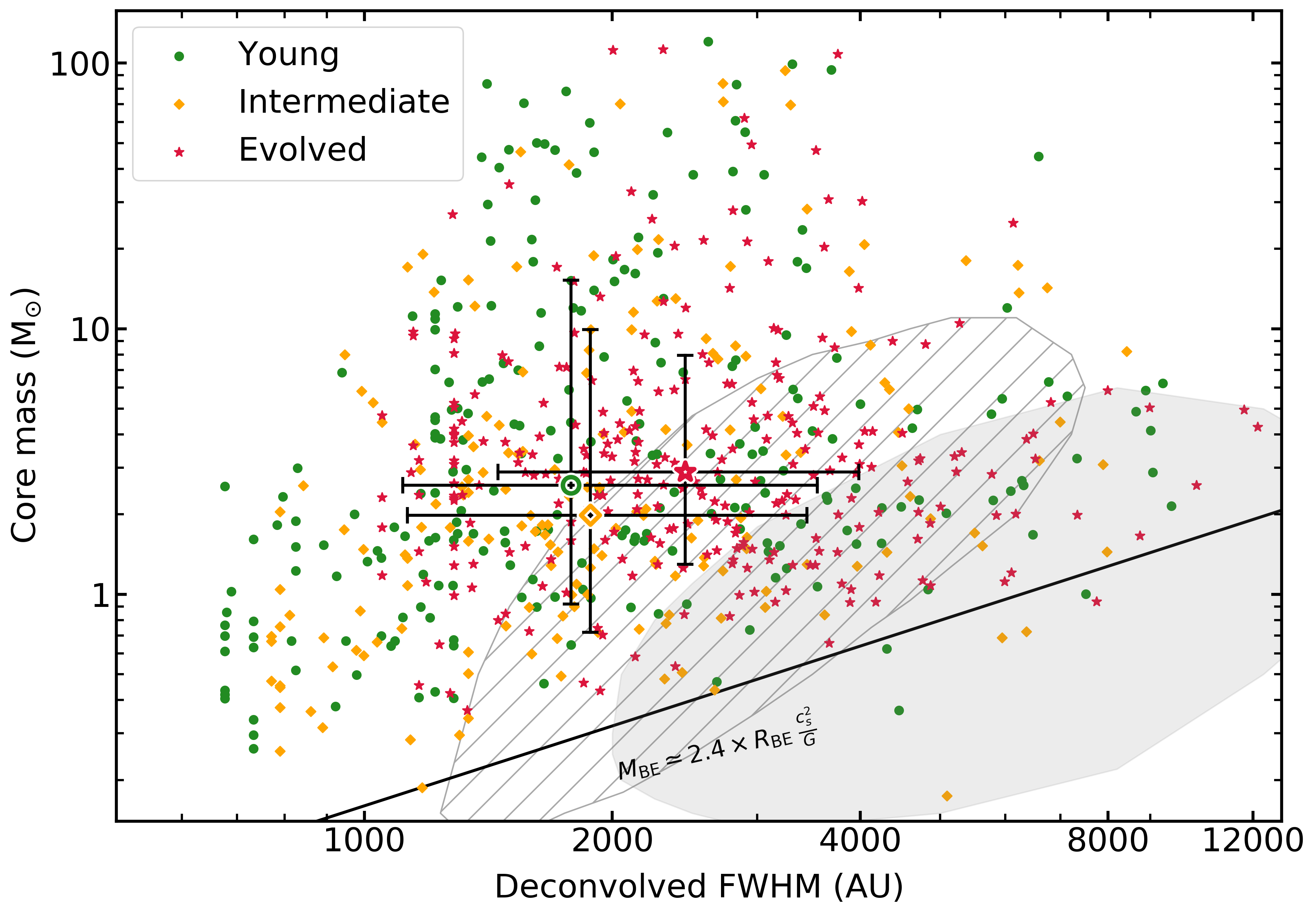
Figure 5: Mass versus size distribution of the ALMA-IMF cores, compared, for reference, to the mass-size relation of critical Bonnor-Ebert spheres for $\mbox{$T_{\rm dust}$}=20$ K (continuous line) and the location of 90% of the core sample of Könyves et al. (2015) and Sanhueza et al. (2019) (dark and light gray shaded areas at the bottom-right corner). The median (open markers) and $1\,\sigma$ dispersion (error bars) of the core distributions for each group of Young (green), Intermediate (orange), and Evolved (red) protocluster clouds are relatively homogeneous. The core FWHMs are deconvolved from the beams, where the minimum deconvolved size corresponds to a half-beam angular diameter and the largest cores are not necessarily the most massive.

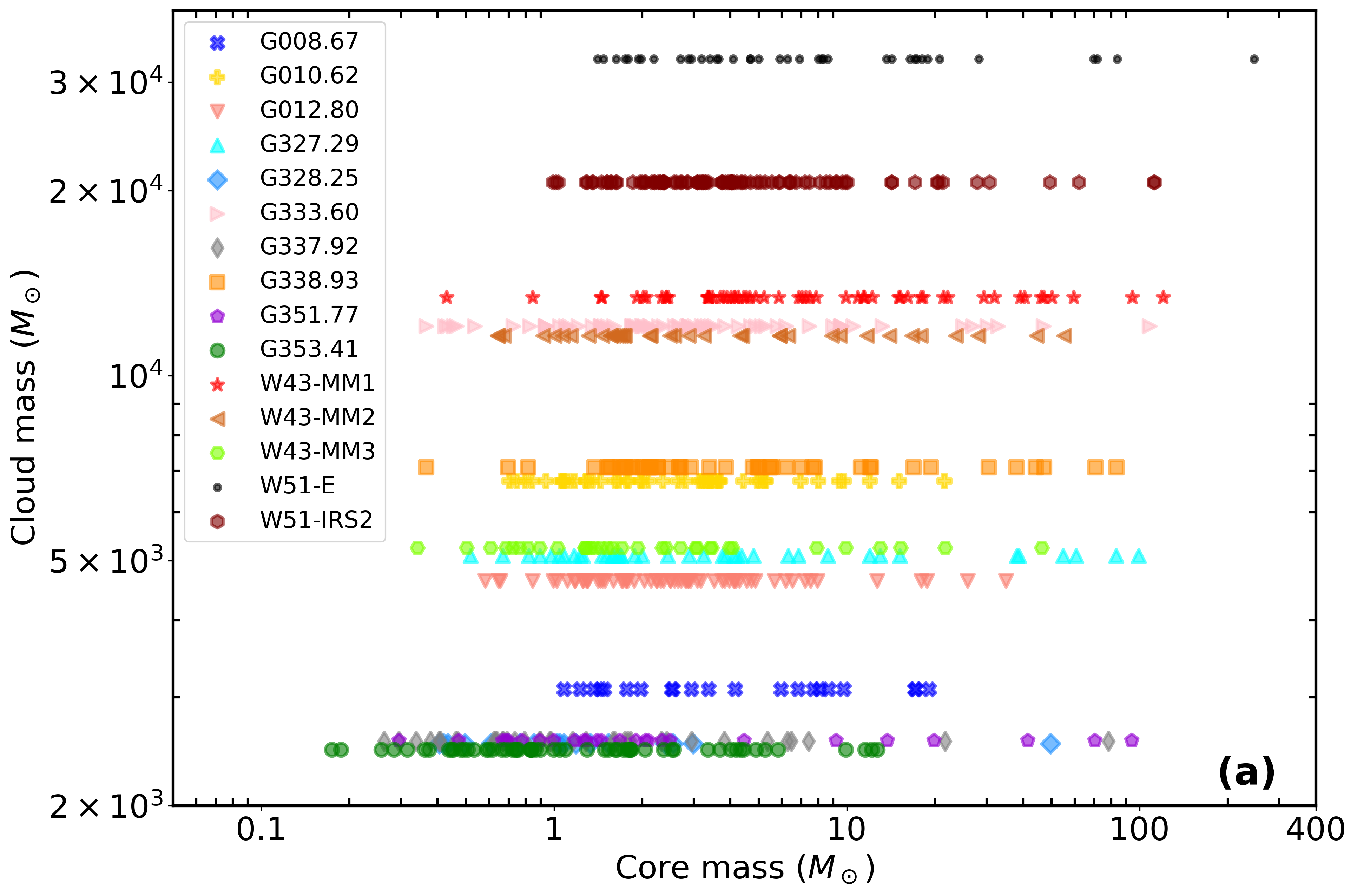
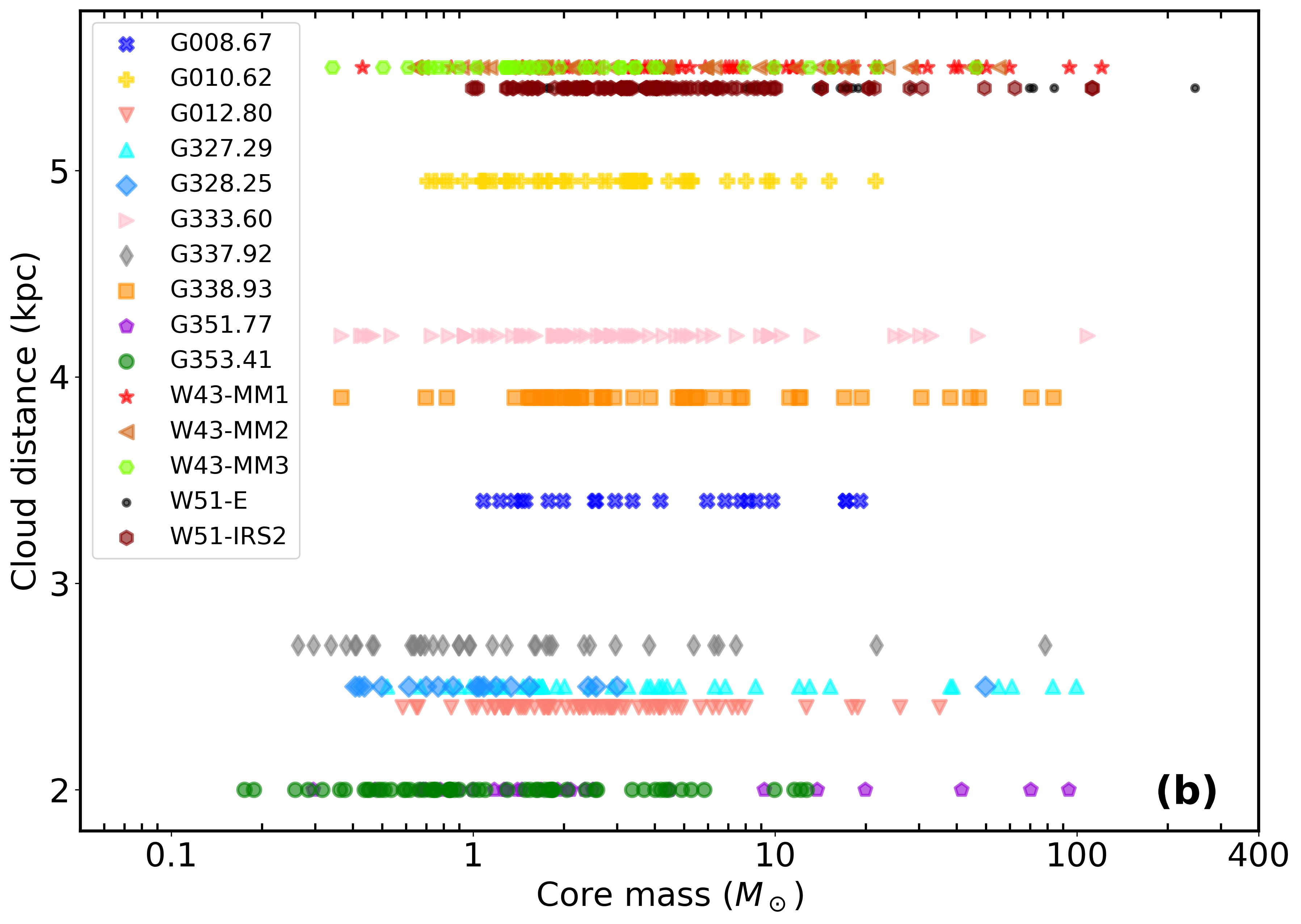
Figure 6: Distribution of the ALMA-IMF core masses as a function of the cloud mass (in a) and distance (in b) of each ALMA-IMF protocluster. The most massive clouds, which also are the farthest, tend to host the most massive cores. The mass sensitivity and, consequently, the lowest-mass core of each core catalog vary by factors of $2.5$. There is no significant bias with the cloud distance to the Sun.

Figure 5 presents the mass-to-size diagram of the $\sim$700 cores extracted in the cleanest continuum images (see catalogs in Louvet et al. in prep., and Table 5). Cores have deconvolved sizes ranging from $\sim$700 au to $\sim$12 000 au, with a median value of $\sim$2 100 au. Their masses span more than three decades, from $\sim$0.15  $M_{\odot}$ to $\sim$250 $M_{\odot}$ and are $\sim$100 times and $\sim$10 times denser than the cores extracted in low-mass star-forming clouds and infrared-dark clouds, respectively (e.g., Könyves et al. 2015; Sanhueza et al. 2019, see Fig. 5). Naively, Fig. 5 implies that the ALMA-IMF cores are gravitationally bound as all cores, with the exception of seven, reside above the thermal value of the critical Bonnor-Ebert mass ($M_{\rm BE}$) for a certain radius ($R_{\rm BE}$), assuming $\mbox{$T_{\rm dust}$}=20$ K:

$$M_{\rm BE}\simeq 2.4\times R_{\rm BE}\,\frac{c_{\rm s}^{2}}{G},$$ (4)

where $c_{\rm s}$ is the isothermal sound speed and $G$ is the gravitational constant. The dynamical state of the cores, however, requires further scrutiny of nonthermal motions associated with turbulence, magnetic fields, and external pressure via the wealth of spectral lines that we detect in ALMA-IMF. Core masses are approximately evenly distributed with size, independent of the evolutionary classification of their host clouds. As shown in Fig. 5, the median sizes and masses of cores in the Young, Intermediate, and Evolved protoclusters are within factors of 14% and 15% of each others, respectively. To more robustly compare the core population of the ALMA-IMF clouds, one should convolve images to the same spatial resolution before extracting cores (see, e.g., Louvet et al. 2021) but this result, derived from images with $2100\pm 400$ au resolutions, already suggests a good degree of homogeneity in terms of cores’ size and mass ranges within the ALMA-IMF cloud sample.

In Fig. 6, we plot the mass of each core as a function of the mass and distance of its parental cloud. While cloud masses span a decade, the ranges of the core masses are similar and do not depend much on the cloud distance or evolutionary stage. The lowest-mass cores detected in the ALMA-IMF protoclusters have masses that depend on the spatial resolution and mass sensitivity of the cleanest images. In the W51 and W43 protocluster clouds, this sensitivity is particularly limited by the small bandwidth used to estimate their line-free continuum emission (Ginsburg et al. in press., see their Figs. 3–4). Interestingly, the most massive ALMA-IMF clouds tend to host the most massive cores, even if the mass of the these cores is computed with a dust temperature of $\mbox{$T_{\rm dust}$}=75$ K. Based on the Spearman’s rank correlation coefficient (Cohen 1988), we find a strong correlation ($\rho_{s}$ = 0.65 and a low probability, $p=0.009$, for no correlation) between the mass of the host clouds and the most massive core in each of them. Lin et al. (2019) found a similar trend for larger cloud structures, while Sanhueza et al. (2019) found no such correlation for cores in a sample of infrared-dark clouds. Given that the latter clouds are five to ten times less massive than the ALMA-IMF clouds, they could either represent earlier stages of protocluster evolution, where the gas is not highly centrally concentrated yet, or they could be progenitors of stellar clusters that are less rich and form stars less massive than the ALMA-IMF protoclusters. Within the ALMA-IMF clouds, we found 79 cores that have masses larger than 16 $M_{\odot}$ and could represent the precursors of high-mass stars, assuming a gas-to-star conversion factor of $50\%$ for these cores. High-mass star precursors could be even more numerous if the core mass reservoirs are fed by inflowing gas from filaments, as suggested by, for example, Motte et al. (2018a) and observed by, for example, Csengeri et al. (2011a); Olguin et al. (2021), or if cores host protostars that have already accreted significant mass. This large number of high-mass star precursors implies, for the ALMA-IMF pc-size clouds, either a high star-formation efficiency (SFE$\>\simeq 22\%$ assuming the IMF of Kroupa 2001) or a lower, more typical, star-formation efficiency with a top-heavy IMF.

The ALMA-IMF core catalog that is summarized in Table 5 and will be published in the companion paper Paper III (Louvet et al. in prep.) is already rich enough to investigate variations in the shape of the CMF. Deeper core extractions will allow individual CMFs to be constructed for all ALMA-IMF protoclusters and even their subregions. ALMA-IMF studies will look for varying CMFs that must be related to (1) the evolutionary stages of clouds determined in Sect. 4.1 and those of sub-clouds as given by the number of protostars versus pre-stellar cores (see Sects. 4.4–4.5), (2) the cloud mass and density structure partly investigated in Fig. 6a and Sect. 4.3, and (3) the cloud kinematics illustrated in Sects. 4.4–4.5. Due to the strategy chosen to image the ALMA-IMF protocluster clouds (see Sect. 3.1), there should not be significant bias in spatial resolution, mass sensitivity, and evolutionary stage with cloud distance (see Fig. 6b).

4.3 Distribution of gas mass from cloud to cores

The distribution of gas mass from the scale of clouds to the scale of cores provides insight into the ability of clouds to form stars, the star-formation efficiency (e.g., Louvet et al. 2014; Nony et al. 2021). Known to depend on the cloud environment in the Milky Way (Nguyen Luong et al. 2011; Veneziani et al. 2013; Kruijssen et al. 2014), the star-formation efficiency also depends on the relationship between stars and their cloud gas reservoir used for protostellar accretion, and therefore between the IMF and the CMF. Gas concentration can be investigated measuring density gradients (e.g., Didelon et al. 2015; Stutz & Gould 2016; Álvarez-Gutiérrez et al. 2021), power spectra of the coherent cloud structures associated with star formation using multi-scale, multi-fractal techniques such as MnGSeg or the reduced wavelet scattering transform (RWST) (Robitaille et al. 2019; Allys et al. 2019), or using less informative functions such as probability distribution functions (e.g., Kainulainen et al. 2013; Schneider et al. 2015; Stutz & Kainulainen 2015). Due to the low spatial dynamic range (i.e., one to two orders of magnitude) of the ALMA-IMF continuum images currently available (12 m array; see Sect. 3.2), we limit our structural study here to ratios of masses measured at three different physical scales.

The mass of each ALMA-IMF cloud and the cumulative mass of their hosted cores are given in Tables 4–5, respectively. In addition to these 1 pc- and 0.01 pc-size cloud and core scale structures, the intermediate-scale structures recovered in the ALMA 1.3 mm 12 m array images mostly consist of clumps or filaments with characteristic sizes close to the largest angular scale discussed in Sect. 3.2 (i.e., $\sim$0.1 pc). For each protocluster, the 1.3 mm fluxes, $S^{\rm recovered}_{\rm 1.3\,mm}$, are integrated over the entire cloud extent, as imaged at 1.3 mm. In the cases of Intermediate and Evolved protocluster clouds, thermal dust emission fluxes are estimated ignoring the 1.3 mm fluxes in areas where the free-free emission dominates (as indicated by H41$\alpha$). The masses of cloud structures recovered by ALMA at 1.3 mm, $M^{\rm recovered}_{\rm 1.3\,mm}$, are then computed from these fluxes, using Section 4.2 and assuming a temperature of $\mbox{$T_{\rm dust}$}=20$ K whatever the evolutionary stage of the clouds.

Table 5 lists the three mass ratios that quantify gas mass concentrations from its cloud to the clumps or filaments (1 pc to 0.1 pc), from clumps or filaments to cores (0.1 pc to 0.01 pc), and from the cloud to its cores. Their absolute values are uncertain, such as mass estimates, by a factor of a few but their relative values possibly by less than 50%. The $M^{\rm recovered}_{\rm 1.3\,mm}/M^{\rm cloud}_{\rm 870\,\mu m}$ ratio measures the percentage of the cloud mass preferentially located within dense filaments and cores. This ratio covers a wide range of values with a median of $\simeq$22% and a $1\,\sigma$ dispersion of $\pm 13\%$. Similar values for the median and dispersion are observed for the concentration of clump or filament mass within cores: $M^{\rm cores}_{\rm 1.3\,mm}/M^{\rm recovered}_{\rm 1.3\,mm}\simeq 22\%$ and $1\,\sigma\simeq\pm 13\%$. The large relative dispersion observed for these two ratios of gas mass concentration, $\frac{13\%}{22\%}\simeq 0.6$, partly arises from differences in the interferometric filtering (see Table 2). However, since the theoretical filtering presents a $1\,\sigma$ relative dispersion of 0.3 (see Sect. 3.2), it cannot be the sole cause of the 0.6 dispersions of the $M^{\rm recovered}_{\rm 1.3\,mm}/M^{\rm cloud}_{\rm 870\,\mu m}$ and $M^{\rm cores}_{\rm 1.3\,mm}/M^{\rm recovered}_{\rm 1.3\,mm}$ mass ratios. Moreover the concentration of the gas mass of clouds into cores, independent of any interferometric filtering, displays values similarly dispersed around its median: $M^{\rm cores}_{\rm 1.3\,mm}/M^{\rm cloud}_{\rm 870\,\mu m}\simeq 4.1\%$ and $1\sigma\simeq\pm 2.6\%$, corresponding to a relative dispersion of 0.6. The variations in gas mass concentration from 1 pc to 0.1 pc and from 0.1 pc to 0.01 pc could therefore trace intrinsic physical variations from one cloud to another. These variations in cloud gas concentration will be investigated in the future in the context of the mass and spatial distributions of cores, and in conjunction with other cloud physical properties (mass, density, turbulence level, and kinematics). When we compare the three subgroups of clouds at different evolutionary stages, we find no significant change in gas mass concentration over time. If confirmed, this result suggests that the cloud structure remains the same in young clouds and parts of evolved clouds outside H ii regions. If the spatial filtering does not change too much our mass ratio measurements, the feedback effects of stars on clouds would therefore remain very limited as long as their H ii regions do not extend over the entire cloud.

(a)

Figure 7: Network of filaments, which interact at the center of the G353.41 protocluster. First-moment (in a) and second-moment (in b) 12 m array images of the N₂H⁺(1-0) isolated hyperfine satellite, corresponding to the centroid velocity and line width. The 1.3 mm continuum emission is overlaid in (a) in black contours, which are 4, 20, 40, 80, and 160 in units of $\sigma=0.3$ mJy beam^-1. Red ellipses in b denote the ALMA-IMF core locations. Ellipses in the lower-left corners represent the angular resolutions of the N₂H⁺(1-0) in a and 1.3 mm continuum images in b.

4.4 Gas kinematics in massive molecular clouds

In dynamical scenarios, molecular clouds are moving structures from birth to death (e.g., Ballesteros-Paredes et al. 2020). They form by the collision of H i gas streams or cloud-cloud collision, they constantly evolve and eventually disperse, notably due to feedback effects such as protostellar outflows, H ii regions, and supernovae. In quasi-static scenarios, on the other hand, clouds are formed by the slow agglomeration of gas, and they evolve little until their dispersion under the effects of stellar feedback (McKee & Ostriker 2007). Observational studies from the past decade have reported intense gas motions on and around filaments: global infall of the gas surrounding filaments (e.g., Williams & Garland 2002; Peretto et al. 2007; Schneider et al. 2010; Galván-Madrid et al. 2010; Jackson et al. 2019; Bonne et al. 2020); oscillations and rotation of filaments (e.g., Stutz & Gould 2016; Álvarez-Gutiérrez et al. 2021); hub-type sub-filament accretion (e.g., Galván-Madrid et al. 2013; Peretto et al. 2013; Nakamura et al. 2014; Treviño-Morales et al. 2019; Chen et al. 2019), braiding of sub-filaments (also called fibers) into filaments or ridges (Schneider et al. 2010; Hennemann et al. 2012; Henshaw et al. 2014; Hacar et al. 2018; González Lobos & Stutz 2019); and local gas infall toward cores (Galván-Madrid et al. 2009; Csengeri et al. 2011a; Olguin et al. 2021). A few studies have also reported large-scale low-velocity shocks in high-mass star-forming regions, traced by SiO molecular line emissions (Jiménez-Serra et al. 2010; Sanhueza et al. 2013; Nguyen-Luong et al. 2013; Louvet et al. 2016). Such emission could emerge as a consequence of the formation of high-mass star-forming regions through cloud-cloud collision.

The ALMA-IMF line data cubes contain several emission lines necessary to trace the gas kinematics (velocity gradients, infall, rotation, turbulence level, and shocks) of cloud structures from the average $\rm 10^{4}\leavevmode\nobreak\ cm^{-3}$ gas density of massive clouds up to the $\rm 10^{7}\leavevmode\nobreak\ cm^{-3}$ density of cores. The Large Program setup indeed notably covers, with increasing critical density ($n_{\rm crit}=1\times 10^{4}-5\times 10^{6}\leavevmode\nobreak\ \rm cm^{-3}$), the C¹⁸O (2-1), N₂H⁺ (1-0), DCO⁺ (3-2), DCN (3-2), N₂D⁺ (3-2), and ¹³CS (5-4) emission lines (see Table 3). The constraints obtained for these different lines, along with shock lines such as SiO (5-4), will be combined in future work to quantify the kinematics of molecular clouds and protoclusters over two orders of magnitude in physical scale, from one parsec to one hundredth of a parsec. The multi-scale kinematics of each ALMA-IMF cloud can then be confronted with theories of global infall, hierarchical collapse, or inertial inflow (e.g., Smith et al. 2009; Vázquez-Semadeni et al. 2019; Padoan et al. 2020) and observational models of rotation, oscillation, or clump-fed accretion (e.g., Braine et al. 2020; Stutz 2018; Motte et al. 2018a).

The first ALMA-IMF studies focus on the N₂H⁺ (1-0) line, which traces gas filaments crossing the protocluster clouds. Figure 7a displays, for the G353.41 protocluster, the line centroid velocity of the isolated hyperfine satellite of the N₂H⁺ (1-0) multiplet ($J\,F_{1}\,F=1\,0\,1\rightarrow 0\,1\,2$, at $\sim$93.176 GHz). With this single piece of information, one can already identify three possible velocity components, separated by $\sim$2 km s^-1. The first one, at $-18\leavevmode\nobreak\ \mbox{km\leavevmode\nobreak\ s${}^{-1}$}$, crosses the cloud from southeast to northwest. The second one, at $-16\leavevmode\nobreak\ \mbox{km\leavevmode\nobreak\ s${}^{-1}$}$, presents a “V” shape from northeast to the center region and finally northwest and the last one, at $-14\leavevmode\nobreak\ \mbox{km\leavevmode\nobreak\ s${}^{-1}$}$, extends from northeast to center. These velocity components are globally filamentary and may represent filaments that interact at the central hub of G353.41, which hosts four intermediate-mass cores ($>$10 $M_{\odot}$; see Fig. 6) including an UCH ii region (see Figs. 2l and 3l; see also Table 4).These filamentary components exhibit significant velocity differences corresponding to a crossing time on the order of $2.5\times 10^{5}\,$Myr (1 pc at 4 km s^-1); they may therefore play an important role in the building up and continued growth of the dense structures of the G353.41 cloud.

Figure 7b presents, for the same isolated hyperfine satellite of the N₂H⁺ (1-0) multiplet, the velocity width of the line consisting of all velocity components and fitted by a single Gaussian. While the line generally appears to have width on the order of $0.5-1.5\leavevmode\nobreak\ \mbox{km\leavevmode\nobreak\ s${}^{-1}$}$, the multiple velocity components observed on the line of sight of the overlapping areas of these filamentary components mimic line broadening with velocity widths larger than 3 km s^-1. Disentangling the multiple velocity components is necessary to properly study the complex dynamics of the region. Overall, the filament network of Fig. 7 is reminiscent of the fan morphology observed for other intermediate- to high-mass hubs (e.g., Peretto et al. 2013; Nakamura et al. 2014; Lu et al. 2018; Treviño-Morales et al. 2019; González Lobos & Stutz 2019). As shown in Fig. 7b, these dense filaments host many continuum cores, with the most massive ones at their potential connection-hub.

A major challenge of the ALMA-IMF project is to quantify the mass growth of cores as a function of environment. The mass of the gas channeled through these filaments should therefore be measured to estimate the mass inflow accretion rates toward each of the detected cores. We started investigating the nature of the cores detected by Louvet et al. (in prep., see also Sect. 4.2). An important goal is to compare pre-stellar and protostellar CMFs, as was done for example by Hatchell & Fuller (2008). To this end, we use the CO (2-1) and SiO (5-4) lines to search for outflows driven by continuum cores; cores with and without outflows are therefore called protostellar and pre-stellar cores, respectively. In parallel, a detailed characterization of the outflows through their CO (2-1) and SiO (5-4) emission will allow us to reach three objectives: reveal the episodicity of the accretion-ejection processes, as done by, e.g., Nony et al. (2020), constrain the turbulence level injected by the outflows into ambient molecular gas on cloud scales (e.g., Li et al. 2020) at the different evolutionary stages, and search for molecular outflows of peculiar morphology (e.g., Tafoya et al. 2021).

Due to the higher sensitivity of future measurements using the wealth of spectral lines (see Table 3 and Sect. 4.5), including the entire N₂H⁺ (1-0) line multiplet in combined 12 m plus 7 m plus Total Power data cubes, the conditions (optical depth, excitation temperature), radial and line-of-sight velocities, and line widths in the ALMA-IMF protoclusters will be determined in detail in future work. In turn, these measurements will permit the evaluation of potential changes in dense gas properties with evolutionary stage (see Sect. 4.1) and core properties (see Sects. 4.2 and 4.5).

Figure 8: ALMA-IMF spectrum, consisting of the 12 spectral windows of the 12 m array data cubes, observed for the brightest 1.3 mm source of the G351.77 protocluster. Located at (RA, Dec)_ICRS=($+17^{h}$26^m42${\hbox to0.0pt{.\hss}{{}^{s}}}51$, $-36^{\circ}09^{\prime}17.53^{\prime\prime}$), this hot core is associated with a core that has a $\sim$15–30 $M_{\odot}$ mass assuming optically thin thermal dust emission at $\mbox{$T_{\rm dust}$}=50-100$ K. The spectra have been converted to a brightness temperature scale in kelvins using the respective synthesized beam values. The brightest spectral lines are identified with colored labels.

4.5 Hot cores and molecular complexity in high- and low-mass protostars

Emission lines of COMs originating from bright hot cores or chemically rich protostars are present over multiple, if not all, ALMA bands. With a 6.4 GHz noncontinuous bandwidth, corresponding to 2.9 GHz covered by four spectral windows at 3 mm plus 3.5 GHz covered in eight spectral windows at 1.3 mm, the ALMA-IMF data will reveal the molecular content of a large population of objects (see Sect. 3.2 and transitions in Fig. 8 and Table 3). Cores extracted in the ALMA-IMF protoclusters cover a broad range of masses, $0.15-250\leavevmode\nobreak\ \mbox{$M_{\odot}$}$, and all evolutionary stages from pre-stellar cores, to protostars, to HCH ii regions (see Sect. 4.2 and Fig. 5). The brightest cores frequently display line-rich spectra associated with hot molecular gas (see, e.g, Fig. 8). Indeed, several well-known hot cores are within the ALMA-IMF images, especially in all the Evolved clouds, G010.62 (Liu et al. 2010; Law et al. 2021), W51-IRS2 (e.g., Henkel et al. 2013), G012.80 (Immer et al. 2014), and G333.6 (Lo et al. 2015). Other well-studied hot cores include those in the Intermediate clouds G351.77 (e.g., Leurini et al. 2008), G008.67 (e.g., Hernández-Hernández et al. 2014), and W51-E (e.g., Zhang et al. 1998; Rivilla et al. 2017) and one in the Young G327.29 cloud (Wyrowski et al. 2008; Bisschop et al. 2013).

A first-look analysis of ALMA-IMF data cubes concerning hot molecular gas indicates that all the targeted protoclusters, even the youngest ones, contain at least one core with line-rich spectra. In particular, the 10 brightest continuum sources from Table 5, corresponding to cores with masses $>$25 $M_{\odot}$ assuming $\mbox{$T_{\rm dust}$}=75$ K (see Sect. 4.2), all exhibit numerous transitions from COMs in all spectral bands and thus are potential hot cores. This trend suggests that the hot core phase would appear very early in the evolutionary sequence of the formation of high-mass stars and massive clusters. While most protoclusters classified as Intermediate or Evolved are associated with known hot cores, several of the youngest ALMA-IMF protoclusters host previously unrecognized (e.g., G337.92 and W43-MM2) or recently identified hot cores (W43-MM1, Molet et al. 2019), or a hot core precursor (G328.25 Csengeri et al. 2019). Figure 8 displays, the complete ALMA-IMF spectrum of the well-known hot core located in the G351.77 protocluster cloud, also known as IRAS 17233$-$3606 (e.g., Leurini et al. 2008). A large number of transitions from COMs commonly observed toward hot cores are clearly detected, the brightest of which originate from the CH₃OH, CH₃CN, CH₃CCH, CH₃OCHO, C₂H₅CN, and CH₃CHO molecules (see Fig. 8). These lines will be used to assess and statistically compare the molecular content of the thousand cores detected by ALMA-IMF (see Table 5). Among these transitions, those of the CH₃OH, CH₃CN, and CH₃CCH molecules can serve as excellent probes of the physical conditions of hot molecular gas (e.g., Gieser et al. 2021). They can be used to estimate kinetic temperatures, column densities and molecular abundances. Temperature estimates based on molecular tracers will put additional constraints on the average dust temperatures, and hence will allow us to better characterize the properties of protostars and improve their mass estimates. Heavier COMs and rotational transitions from vibrationally excited states such as CH₃CN ($v_{8}=1$) in Fig. 8 should be detected toward some of the most massive ALMA-IMF cores, thus providing further constraints on their excitation conditions.

The sensitivity of the ALMA-IMF data cubes at 1.3 mm reaches about 0.5–1 K at 1 km s^-1 resolution (see Sect. 3.2 and Fig. 8). This sensitivity is largely sufficient to detect, in the ALMA-IMF clouds, a hot core such as Orion-KL that exhibits spectral lines with peak brightness temperatures of $\sim$20-30 K in a 2000 au beam (e.g., Brouillet et al. 2015; Pagani et al. 2017). Archetypical hot corinos, such as IRAS 16293 or IRAS 4A with sizes of at most a few 100 au (Jørgensen et al. 2016; Belloche et al. 2020), would themselves remain undetected in our survey because of the large beam dilution. Preliminary investigations of the ALMA-IMF data cubes suggest, however, that line transitions typical of hot cores are detected toward cores of low to intermediate masses (i.e., $2-4\leavevmode\nobreak\ \mbox{$M_{\odot}$}$; e.g., Motte et al. 2018b). Altogether, based on a first look analysis of the detection rates of COMs toward cores of the W43-MM1, W43-MM2, and W43-MM3 protoclusters (Brouillet et al. in prep.), we expect to identify one to five cores with line-rich spectra in each ALMA-IMF cloud, giving statistics of $15-75$ high-mass and intermediate-mass hot cores.

The advantage of the ALMA-IMF survey to study the molecular complexity is that it provides a large sample of hot cores and various cloud environments undergoing dynamical events (gas inflow and protostellar outflows; see Sect. 4.4), all studied with the same physical scale, sensitivity, and spectral coverage. Recent studies of molecular complexity show that, in addition to the classical radiative heating corresponding to hot cores, a range of physical processes may lead to the emergence of emission from COMs. For example, significant amounts of COMs are released in the gas phase through shocks created by protostellar outflows (such as L1157-B1 and IRAS 4A, e.g., Lefloch et al. 2017; De Simone et al. 2020), in externally heated regions (such as Orion-KL and photodissociation regions; Favre et al. 2011; Pagani et al. 2019; Le Gal et al. 2017), and through accretion shocks (as observed toward G328.25, Csengeri et al. 2019). Beyond the emergence of COMs, ALMA-IMF also covers several deuterated molecules as well as isotopologues from abundant species such as CH₃CN, CH₃OH, OCS, and H₂CO. Measurements of the deuteration and isotopic fractionation provide indications of physical conditions that may impact the chemistry. Therefore, the physical processes and the chemistry driving the emergence of molecular complexity in high-mass protostars and dynamically evolving clouds could be statistically established with ALMA-IMF and then further compared to chemical models (see Garrod & Herbst 2006; Ruaud et al. 2016; Holdship et al. 2017). This goal is particularly important for emerging hot cores, as they offer excellent laboratories to study the early warm-up phase chemistry.

5 Conclusion

ALMA-IMF is a Cycle 5 Large Program carried out with ALMA 12 m, 7 m, and Total Power arrays. Its potential and first highlights based on 12 m array data can be summarized as follows:

1. We selected 15 massive ($2-33\times 10^{3}\leavevmode\nobreak\ \mbox{$M_{\odot}$}$), nearby ($2.5-5.5$ kpc) protoclusters that span early protocluster evolutionary stages (see Sect. 2 and Table 1). ALMA mosaics cover total noncontiguous areas of $\sim$53 pc² at 1.3 mm and $\sim$122 pc² at 3 mm in the typical yet extreme environments of the Milky Way clusters in formation (see Fig. 1). The ALMA-IMF spectral setup was carefully designed to focus on lines tracing gas motions from clouds to cores. In addition, the ALMA-IMF setup covers a 6.4 GHz noncontinuous bandwidth at 3 mm (Band 3, 99.66 GHz) and 1 mm (Band 6, 228.4 GHz) used to survey lines from COMs.

2. The ALMA-IMF data set is homogeneous, with approximately matched point mass sensitivity and physical resolution across the protocluster sample that spans a factor of $\sim$3 in distance. Hence, the key feature of our approach is the lack of significant distance bias, which enables robust, synergistic science on the emergence of the IMF and star clusters. The ALMA-IMF database consists of 1 mm and 3 mm continuum images that are sensitive to $\sim$0.18 $M_{\odot}$ and $\sim$0.6 $M_{\odot}$ point-like cores, respectively, at a matched spatial resolution of $\sim$2 100$\pm 400$ au (see, e.g., Fig. 3). Moreover, the ALMA-IMF data set contains many emission lines that trace dense molecular gas, outflows, shocks, COMs probing hot cores, and recombination lines that trace the ionized gas (see Sect. 3 and Table 3). The whole ALMA-IMF data set is processed with a pipeline described in Paper II (Ginsburg et al. in press.), in which we have carried out a homogeneous, repeatable, and high-quality reduction.

3. We improved the evolutionary stage classification of the 15 protoclusters based on visual inspection and quantitative measurements of the distribution of free-free and thermal emission (see Sect. 4.1 and Table 4). Four protoclusters are classified as Evolved based on their advanced H ii activity compared to the other sources in our sample. They present strong, complex, and extended free-free emission traced by the H41$\alpha$ line and 3 mm continuum (see Figs. 3l–o and 4). Six protoclusters are classified as Young based on being devoid of internal ionizing sources (see Figs. 3a–f and 4), with free-free emission two orders of magnitude smaller than those measured for Evolved clouds. In between these extrema, Intermediate protoclusters host both dense filamentary structures traced by their thermal dust emission and small, localized bubbles of ionized gas (see Figs. 3g–k and 4).

4. The ALMA-IMF core catalog contains $\sim$700 cores spanning $\sim$0.15 $M_{\odot}$ to $\sim$250 $M_{\odot}$, with a median size of $\sim$2 100 au (see Fig. 5, Table 5, and Sect. 4.2). This core sample, published in Paper III (Louvet et al. in prep.), has no significant bias with cloud distance or cloud evolutionary stage (see Figs. 5-6). Within the ALMA-IMF clouds, we found 79 cores that have masses larger than 16 $M_{\odot}$, which could represent the precursors of high-mass stars, assuming a gas-to-star conversion factor of $50\%$ for these cores. The most massive protocluster clouds tend to host the most massive cores, even if the masses of such cores are computed with a dust temperature of $\mbox{$T_{\rm dust}$}=75$ K (see Fig. 6). Core catalogs of Louvet et al. (in prep.) will be used to build CMFs and study their variations with cloud characteristics and evolutionary stage.

5. ALMA-IMF has the ability to constrain the distribution of gas mass from the scale of clouds to the scale of cores and thus provide insight into the star-formation efficiency. Due to the current dynamic range, however, we limit our structural analysis to mass ratios that quantify the gas mass concentration from cloud to clumps or filaments (1 pc to 0.1 pc), from clumps or filaments to cores (0.1 pc to 0.01 pc), and from cloud to cores (see Table 5). Initial results on the concentration of cloud gas into cores suggest that stellar feedback has little effect on the structure development of high-density gas (see Sect. 4.3).

6. The ALMA-IMF line data cubes contain all the emission lines necessary to trace the gas kinematics (velocity gradients, infall, rotation, turbulence level, and shocks) of cloud structures from the average $\rm 10^{4}\leavevmode\nobreak\ cm^{-3}$ gas density of massive clouds up to the $\rm 10^{7}\leavevmode\nobreak\ cm^{-3}$ density of cores (see Table 3 and Sect. 4.4). The constraints obtained for these different lines, along with shock tracing lines such as SiO (5-4), will be combined to quantify the kinematics of molecular clouds and protoclusters over two orders of magnitude in physical scale, from one parsec to one-hundredth of a parsec. In particular, the N₂H⁺ (1-0) line shows networks of filaments that may trace inflow gas streamers (see, e.g., Fig. 7). They will be traced down to the scale of cores to potentially quantify the growth of core masses and the evolution over time of the shape of the CMF.

7. ALMA-IMF has the potential to identify several tens of cores that exhibit line-rich spectra potentially corresponding to hot cores (see, e.g., Fig. 8 and Sect. 4.5). Beyond the well-known hot cores hosted in Evolved protoclusters, we also cover several regions where completely new, bright hot cores can be recognized. The detection of COMs toward the brightest sources suggests that the hot core phase appears early in the emergence of high-mass protostars. Thanks to the similar sensitivity and spatial resolution toward each protocluster, we will be able to perform a homogeneous characterization of their molecular content and use spectroscopic tracers to constrain the emerging molecular complexity in protostars of high to intermediate mass.

The ultimate objective of ALMA-IMF is to push forward our understanding of the IMF of stars and stimulate improvements to star-formation models, taking the effects of cloud characteristics and evolution into account. To this end, we will provide the community with a high-legacy database of protocluster clouds, filaments, cores, hot cores, outflows, and inflows at matched sensitivity. We emphasize that ALMA-IMF spans a Milky Way-relevant sample that captures the range in gas mass and evolutionary stages necessary to achieve this legacy value.

Appendix A The most massive ATLASGAL clumps at 2-5.5 kpc

Figure 9 presents the basic characteristics of the ALMA-IMF clumps, taken from the catalog of Csengeri et al. (2017). Table 6 lists the most extreme clumps from the Csengeri et al. (2017) catalog. This list served as a first step in our source selection. In addition to the source position and association to molecular complexes and IRAS sources, we also list projects from the ALMA archive that cover these positions.

Figure 9: Mass versus size distribution of the ATLASGAL clumps selected for the ALMA-IMF survey (highlighted with squares; see Fig. 1), compared to the rest of the Csengeri et al. (2017) sample at distances between 1 kpc and 5.5 kpc. ATLASGAL clumps targeted by ALMA-IMF are among the brightest and most concentrated. For more details on the selection criteria, see Sect. 2.

[c]

Table 6: Massive ATLASGAL clumps that have $S^{\rm int}_{\rm 870\mu m}>25$ Jy fluxes and are located between 2 kpc and 5.5 kpc from the Sun.

ATLASGAL & common1	$d$	Ref.2	Evolutionary	$S^{\rm int}_{\rm 870\mu m}$3	ALMA	Molecular
names	[kpc]	$d$	stage3	[Jy]	projects 4	complex5
G049.4888-0.3882 / W51-E / W51 Main	5.4$\pm 0.3$	(1)	IR-bright	113.2	(1), (8a,b), (9)	W51
					(10), (11), (12)
G333.6036-0.2130 / G333.60 / IRAS 16183-4958	4.2$\pm 0.7$	(2)	IR-bright	97.4	(1)	RCW106
G012.8057-0.1994 / G012.80 / W33-IRS3	2.4$\pm 0.2$	(3)	IR-bright	92.4	(1), (5a)	W33
G351.7747-0.5369 / G351.77 / IRAS 17233-3606	2.0$\pm 0.7$	(4)	IR-bright	81.8	(1), (3), (13), (14)	G353
G327.2921-0.5792 / G327.29 / RCW97	2.5$\pm 0.5$	(2)	IR-bright	71.2	(1), (15)	G327
G353.4102-0.3611 / G353.41 / IRAS 17271-3439	2.0$\pm 0.7$	(4)	IR-bright	68.4	(1) , (3)	G353
G010.6237-0.3833 / G010.62 / W31	4.95$\pm 0.5$	(5)	IR-bright	54.9	(1), (5a) , (14b)	W31
					(16), (17)
G333.1341-0.4314 / IRAS 16172-5028	4.2$\pm 0.7$	(2)	IR-bright	54.2	(2), (3), (4)	RCW106
G338.9249+0.5539 / G338.92	3.9$\pm 1.0$	(2)	IR-quiet	53.3	(1), (2), (18)
G049.4897-0.3697 / W51-IRS2 / IRAS 19213+1424	5.4$\pm 0.3$	(1)	IR-bright	52.0	(1), (8a,b), (10)	W51
G332.8262-0.5493 / IRAS 16164-5046	4.2$\pm 0.7$	(2)	IR-bright	51.4	(2), (5a), (3)	RCW106
G348.7260-1.0391 / IRAS 17167-3854	3.4$\pm 0.3$	(6)	IR-bright	43.4	(2)	RCW122
G030.8166-0.0561 / W43-MM1	5.5$\pm 0.4$	(7)	IR-quiet	42.3	(1), (19a,b)	W43
					(20a,b), (21)
G328.8087+0.6328 / IRAS 15520-5234	2.5$\pm 0.5$	(2)	IR-bright	40.6		G327
G333.2841-0.3868	4.2$\pm 0.7$	(2)	IR-bright	37.5	(2), (4)	RCW106
G049.4908-0.3792 / W51-Main	5.4$\pm 0.3$	(1)	IR-bright	36.9	(1) in W51-E field	W51
G337.9154-0.4773 / G337.92 / IRAS16274-4701	2.7$\pm 0.7$	(4)	IR-bright	36.6	(1), (5a), (5b), (6),	G337
G301.1365-0.2256 / IRAS 12326-6245	4.2$\pm 0.7$	(2)	IR-bright	34.5	(2), (5), (3)
G327.3005-0.5509 / IRAS 15492-5426	2.5$\pm 0.5$	(2)	IR-bright	32.3		G327
G337.4052-0.4024 / IRAS 16351-4722	2.7$\pm 0.7$	(5)	IR-bright	31.7	(2), (5b), (3), (6)	G337
G008.6702-0.3557 / G008.67	3.4$\pm 0.3$	(2)	IR-quiet	30.6	(1), (5b), (22)
G322.1581+0.6354 / RCW92	3.2$\pm 1.1$	(2)	IR-bright	30.3
G329.0303-0.2022 / IRAS 15566-5304	2.5$\pm 0.5$	(2)	IR-quiet	29.4	(3)	G327
G330.8788-0.3681 / IRAS 16065-5158	4.2$\pm 0.7$	(2)	IR-quiet	28.1		RCW106
G019.6084-0.2346 / IRAS 18248-1158	3.6$\pm 0.8$	(2)	IR-bright	27.6	(7)
G326.6577+0.5941 / IRAS 15408-5356 / RCW95	2.5$\pm 0.5$	(2)	IR-bright	26.2		G327
G305.2083+0.2063 / IRAS 13079-6218	3.5$\pm 2.0$	(8)	IR-bright	26.1	(2), (3), (4)
G030.7016-0.0672 / W43-MM2	5.5$\pm 0.4$	(7)	IR-quiet	25.1	(1), (20c)	W43
G328.2551-0.5321 / G328.25	2.5$\pm 0.5$	(2)	IR-quiet	15.0	(1), (23)	G327
G030.7173-0.0822 / W43-MM3	5.5$\pm 0.4$	(7)	IR-bright	11.7	(1), (2), (20c)	W43

• ATLASGAL name (underlying their Galactic coordinates) from Csengeri et al. (2017) together with adopted name for ALMA-IMF (underlined names) as well as other most common names.

• References for the distance to the Sun: (1) Sato et al. (2010); (2) Csengeri et al. (2017); (3) Immer et al. (2013); (4) This paper ; (5) Sanna et al. (2014); (6) Reid et al. (2014); (7) Zhang et al. (2014); (8) Russeil (2003).

• Evolutionary stage and 870 $\mu$m integrated fluxes, taken from Csengeri et al. (2017).

• Observed as part of the: (1) ALMA-IMF Large Program #2017.1.01355.L, by Motte, Ginsburg, Louvet, Sanhueza et al. (B6+B3 mosaics); (2) Large Program #2019.1.00195.L (B6) by Molinari, Schilke et al.; (3) Program by Liu et al. #2019.1.00685.S (B3); (4) Program by Barnes et al. #2019.1.01031.S (B3, mosaic); (5) Programs by Leurini et al. a) #2016.1.01347.S, b) #2017.1.00377.S (B6+B3, mosaics); (6) Program by Hacar et al. #2018.1.00697.S (B3, mosaic); (7) Program by Se-Hyung et al. #2013.1.00266.S (B3); (8) Programs by Ginsburg et al. a) #2013.1.00308.S (B6, mosaic) and b) #2017.1.00293.S (B3); (9) Program by Kim et al. #2015.1.01571.S (B6); (10) Program by Goddi et al. #2015.1.01596.S (B6); (11) Program by Su et al. #2016.1.00268.S (B3); (12) Program by Rivilla et al. #2016.1.01071.S (B3); (13) Program by Beuther et al. #2015.1.00496.S (B6); (14) Program by Sanhueza et al. a) #2017.1.00237.S and b) #2016.1.01036.S (B6); (15) Program by Schilke et al. #2016.1.00168.S (B6, mosaic); (16) Program by Gerin et al. #2013.1.01194.S (B3); (17) Program by Zhang et al. #2015.1.00106.S (B6); (18) Program by Fuller et al. #2015.1.01312.S (B6); (19) Program by Motte et al. a) #2013.1.01365.S (B6, mosaic) and b) #2015.1.01273.S (B6, mosaic); (20) Program by Louvet et al. a) #2015.1.01020.S (B6), b) #2018.1.01787.S (B3) and c) #2017.1.00226; (21) Program by Kim et al. #2018.1.01288.S (B6); (22) Program by Shirley et al. #2017.1.01116.S (B3, B6); (23) Program by Csengeri et al. #2019.2.00093.S (B3).

• Name of the molecular cloud complex hosting the ATLASGAL clump.