One size does not fit all: Investigating strategies for differentially-private learning across NLP tasks

Abstract

Preserving privacy in contemporary NLP models allows us to work with sensitive data, but unfortunately comes at a price. We know that stricter privacy guarantees in differentially-private stochastic gradient descent (DP-SGD) generally degrade model performance. However, previous research on the efficiency of DP-SGD in NLP is inconclusive or even counter-intuitive. In this short paper, we provide an extensive analysis of different privacy preserving strategies on seven downstream datasets in five different ‘typical’ NLP tasks with varying complexity using modern neural models based on BERT and XtremeDistil architectures. We show that unlike standard non-private approaches to solving NLP tasks, where bigger is usually better, privacy-preserving strategies do not exhibit a winning pattern, and each task and privacy regime requires a special treatment to achieve adequate performance.

1 Introduction

In a world where ‘data is the new oil’, preserving individual privacy is becoming increasingly important. However, modern neural networks are vulnerable to privacy attacks that could even reveal verbatim training data (Carlini et al., 2020). An established method for protecting privacy using the differential privacy (DP) paradigm (Dwork and Roth, 2013) is to train networks with differentially private stochastic gradient descent (DP-SGD) (Abadi et al., 2016). Although DP-SGD has been used in language modeling (McMahan et al., 2018; Hoory et al., 2021), the community lacks a thorough understanding of its usability across different NLP tasks. Some recent observations even seem counter-intuitive, such as the non-decreasing performance at extremely strict privacy values in named entity recognition (Jana and Biemann, 2021). As such, existing research on the suitability of DP-SGD for various NLP tasks remains largely inconclusive.

We thus ask the following research questions: First, which models and training strategies provide the best trade-off between privacy and performance on different NLP tasks? Second, how exactly do increasing privacy requirements hurt the performance? To answer these questions, we conduct extensive experiments on seven datasets over five tasks, using several contemporary models and varying privacy regimes. Our main contribution is to help the NLP community better understand the various challenges that each task poses to privacy-preserving learning.

2 Related work

Differential privacy formally guarantees that the probability of leaking information about any individual present in the dataset is proportionally bounded by a pre-defined constant $\varepsilon$, the privacy budget. We briefly sketch the primary ideas of differential privacy and DP-SGD. For a more detailed introduction please refer to Abadi et al. (2016); Igamberdiev and Habernal (2022); Habernal (2021, 2022).

Two datasets are considered neighboring if they are identical, apart from one data point (e.g., a document), where each data point is associated with one individual. A randomized algorithm $\mathcal{M}:\mathcal{X}\rightarrow\mathcal{Y}$ is $(\varepsilon,\delta)$-differentially private if the following probability bound holds true for all neighboring datasets $x,x^{\prime}\in\mathcal{X}$ and all $y\in\mathcal{Y}$:

$$\Pr\left(\ln\left[\frac{\text{Pr}(\mathcal{M}(x)=y)}{\text{Pr}(\mathcal{M}(x^{\prime})=y)}\right]>\varepsilon\right)\leq\delta,$$ (1)

where $\delta$ is a negligibly small constant which provides a relaxation of the stricter $(\varepsilon,0)$-DP and allows for better composition of multiple differentially private mechanisms (e.g. training a neural model over several epochs). The above guarantee is achieved by adding random noise to the output of $\mathcal{M}$, often drawn from a Laplace or Gaussian distribution. Overall, this process effectively bounds the amount of information that any one individual can contribute to the output of mechanism $\mathcal{M}$.

When using differentially private stochastic gradient descent (DP-SGD) (Abadi et al., 2016), we introduce two additional steps to the standard stochastic gradient descent algorithm. For a given input $x_{i}$ from the dataset, we obtain the gradient of the loss function $\mathcal{L}(\theta)$ at training time step $t$, $g_{t}(x_{i})=\nabla_{\theta_{t}}\mathcal{L}(\theta_{t},x_{i})$. We then clip this gradient by $\ell_{2}$ norm with clipping threshold $C$ in order to constrain its range, limiting the amount of noise required for providing a differential privacy guarantee.

$$\bar{g}_{t}(x_{i})=\frac{g_{t}(x_{i})}{\max\left(1,\frac{||g_{t}(x_{i})||_{2}}{C}\right)}$$ (2)

Subsequently, we add Gaussian noise to the gradient to make the algorithm differentially private. This DP calculation is grouped into ‘lots’ of size $L$.

$$\tilde{g}_{t}=\frac{1}{L}(\sum_{i\in L}\bar{g}_{t}(x_{i})+\mathcal{N}(0,\sigma^{2}C^{2}\mathbf{I}))$$ (3)

The descent step is then performed using this noisy gradient, updating the network’s parameters $\theta$, with learning rate $\gamma$.

$$\theta_{t+1}=\theta_{t}-\gamma\tilde{g}_{t}$$ (4)

In NLP, several works utilize DP-SGD, primarily for training language models. Kerrigan et al. (2020) study the effect of using DP-SGD on a GPT-2 model, as well as two simple feed-forward networks, pre-training on a large public dataset and fine-tuning with differential privacy. Model perplexities are reported on the pre-trained models, but there are no additional experiments on downstream tasks. McMahan et al. (2018) train a differentially private LSTM language model that achieves accuracy comparable to non-private models. Hoory et al. (2021) train a differentially private BERT model and a privacy budget $\varepsilon=1.1$, achieving comparable accuracy to the non-DP setting on a medical entity extraction task.

Only a few works investigate DP-SGD for downstream tasks in NLP. Jana and Biemann (2021) look into the behavior of differential privacy on the CoNLL 2003 English NER dataset (Tjong Kim Sang and De Meulder, 2003). They find that no significant drop occurs, even when using low $\varepsilon$ values such as 1, and even as low as 0.022. This is a very unusual result and is assessed in this work further below. Bagdasaryan et al. (2019) apply DP-SGD to sentiment analysis of Tweets, reporting a very small drop in accuracy with epsilons of 8.99 and 3.87. With the state of the art only evaluating on a limited set of tasks and datasets, using disparate privacy budgets and metrics, there is a need for a more general investigation of the DP-SGD framework in the NLP domain, which this paper addresses.

3 Experimental setup

3.1 Tasks and dataset

We experiment with seven widely-used datasets covering five different standard NLP tasks. These include sentiment analysis (SA) of movie reviews (Maas et al., 2011) and natural language inference (NLI) (Bowman et al., 2015) as text classification problems. For sequence tagging, we explore two tasks, in particular named entity recognition (NER) on CoNLL’03 (Tjong Kim Sang and De Meulder, 2003) and Wikiann (Pan et al., 2017; Rahimi et al., 2019) and part-of-speech tagging (POS) on GUM (Zeldes, 2017) and EWT (Silveira et al., 2014). The third task type is question answering (QA) on SQuAD 2.0 (Rajpurkar et al., 2018). We chose two sequence tagging tasks, each involving two datasets, to shed light on the surprisingly good results on CoNLL in (Jana and Biemann, 2021). Table 1 summarizes the data statistics.

Task	Dataset	Size	Classes
SA	IMDb	50k documents	2
NLI	SNLI	570k pairs	3
NER	CoNLL’03	$\approx$ 300k tokens	9
NER	Wikiann	$\approx$ 320k tokens	7
POS	GUM	$\approx$ 150k tokens	17
POS	EWT	$\approx$ 254k tokens	17
QA	SQuAD 2.0	150k questions	$\star$

Table 1: Datasets and their specifics. $\star$ SQuAD contains 100k answerable and 50k unanswerable questions, where answerable questions are expressed as the span positions of their answer.

3.2 Models and training strategies

We experiment with five different training (fine-tuning) strategies over two base models. As a simple baseline, we opt for (1) Bi-LSTM to achieve compatibility on NER with previous work (Jana and Biemann, 2021). Further, we employ BERT-base with different fine-tuning approaches. We add (2) LSTM on top of frozen BERT encoder (Fang et al., 2020) (Tr/No/LSTM), a (3) simple softmax layer on top of ‘frozen’ BERT (Tr/No), and the same configuration with (4) fine-tuning only the last two layers of BERT (Tr/Last2) and finally (5) fine-tuning complete BERT without the input embeddings layer (Tr/All).

In contrast to the non-private setup, the number of trainable parameters affects DP-SGD, since the required noise grows with the gradient size. Therefore we also run the complete experimental setup with a distilled transformer model XtremeDistilTransformer Model (XDTM) Mukherjee and Hassan Awadallah (2020). Details of the privacy budget and its computation, as well as hyperparameter tuning are in Appendix A and B.

4 Analysis of results

As LSTM performed worst in all setups, we review only the transformer-based models in detail. Also, we discuss only $\varepsilon$ of $1.0,5.0,$ and $\infty$ (non-private) as three representative privacy budgets. Here we focus on the BERT-based scenario; a detailed analysis of the distilled model XDTM is provided in Appendix E. Random and majority baselines are reported only in the accompanying materials, as they only play a minor role in the drawn conclusions. All results are reported as macro-$F_{1}$ (averaged $F_{1}$ of all classes). We additionally provide an analysis of efficiency and scalability in Appendix C and an analysis on optimal learning rates in Appendix D.

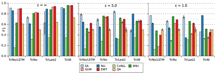
Figure 1: Macro $F_{1}$ scores for non-private ($\varepsilon=\infty$) and two private configurations ($\varepsilon\in\{5;1\}$) grouped by a particular model (x-axis). Each column represents the score for a specific task performed by the corresponding model. When analyzing one task (one column) in the non-private ($\varepsilon$=$\infty$) setting for different models, macro $F_{1}$ increases when adding fine-tuning. In DP models, no clear pattern can be observed and the best model is task specific. A complementary task-specific chart with performance drops is shown in Fig. 3 in the Appendix.

4.1 Sentiment analysis

Binary sentiment analysis (positive, negative) is a less complex task. Unsurprisingly, all non-private models achieve good results (Figure 1 left). Moreover, each model — except for the fully fine-tuned BERT model Tr/All — shows only a small performance drop with DP.

Why fine-tuning full BERT with DP-SGD fails?

While fully fine-tuned BERT is superior in non-private setups, DP-SGD behaves unexpectedly. Instead of having more varied predictions with increasing DP noise, it simply predicts everything as negative with $F_{1}=0.46$, even though the training data is well-balanced (see the confusion matrix in Table 5 in the appendix). However, fine-tuning only the last two layers (Tr/Last2) achieves $F_{1}>0.7$. This seems to be consistent with the observation that semantics is spread across the entire BERT model, whereas higher layers are task specific (Rogers et al., 2020, Sec. 4.3), and that sentiment might be well predicted by local features (Madasu and Anvesh Rao, 2019) which are heavily affected by the noise.

4.2 Natural Language Inference

As opposed to sentiment analysis, NLI results show a different pattern. In the non-private setup, two models including fine-tuning BERT, namely Tr/Last2 and Tr/All, outperform other models. This is not the case for DP training.

What happened to BERT with DP on the last layers?

Fine-tuning only the last two layers (Tr/Last2) results in the worst performance in private regimes, e.g., for $\varepsilon=1$ (Fig. 1 right). Analyzing the confusion matrix shows that this model fails to predict neutral entailment, as shown in Table 2 top. We hypothesize that the DP noise destroys the higher, task-specific BERT layers, and thus fails on the complexity of the NLI task, that is to recognize cross-sentence linguistic and common-sense understanding. Furthermore, it is easier to recognize entailment or contradiction using some linguistic shortcuts, e.g., similar words pairs, or dataset artifacts (Gururangan et al., 2018).

Full fine-tuning BERT (Tr/All) yields the best private performance, as can be also seen in Table 2 bottom. This shows that noisy gradient training spread across the full model increases robustness for the down-stream task which, unlike sentiment analysis, might not heavily depend on local features, e.g., word n-grams.

	$\downarrow$ gold	Entail.	Contrad.	Neutral
Tr/Last2	Entail.	1356	1699	313
	Contrad.	1122	1780	335
	Neutral	1217	1677	325
Tr/All	Entail.	2832	129	407
	Contrad.	272	2530	435
	Neutral	375	604	2240

Table 2: Confusion matrices for $\varepsilon=1$ on NLI.

4.3 NER and POS-Tagging

While the class distribution of SA and NLI is well-balanced, the four datasets chosen for the two sequence tagging tasks are heavily skewed (see Tables 7 and 8 in the Appendix). Our results show that this imbalance negatively affects all private models. The degradation of the underrepresented class is known in the DP community. Farrand et al. (2020) explore different amounts of imbalances and the effect on differentially private models. Bagdasaryan et al. (2019) find that an imbalanced dataset has only a small negative effect on accuracy for the underrepresented class when training in the non-private setting but it degrades when adding differential privacy. Both NER and POS-tagging behave similarly when being exposed to DP, as only the most common tags are well predicted, namely the outside tag for NER and the tags for noun, punctuation, verb, pronoun, adposition, and determiner for POS-tagging. Tables 9 and 10 in the Appendix show the large differences in $F_{1}$-scores with $\varepsilon=1$.

Drawing conclusions using unsuitable metrics?

While the average of all class $F_{1}$-scores (macro $F_{1}$-score) suffers from wrong predictions of underrepresented classes, accuracy remains unaffected. Therefore we suggest using macro $F_{1}$ to evaluate differential private models which are trained on imbalanced datasets. The difference in accuracy-based metric and macro $F_{1}$ score explains the unintuitive invariance of NER to DP in (Jana and Biemann, 2021).

Non-private NER misclassifies prefix but DP fails on tag type.

Further inspection of the NER results reveals that without DP, the model tends to correctly classify the type of tag (e.g. loc, per, org, misc) but sometimes fails with the position (i, b prefix). This can be seen in the confusion matrix (Table 11 in the Appendix), examples being i-loc very often falsely classified as b-loc or i-per as b-per. The same pattern is present for i-org, and i-misc. However, DP affects the models’ predictions even further, as now, additionally to the position, the tag itself gets wrongly predicted. To exemplify, i-misc is falsely predicted as b-loc 502 times and i-org as b-loc 763 times, as can be seen in Table 12 in the Appendix.

NER is majority-voting with meaningful $\varepsilon$ already, turns random only with very low $\varepsilon$.

As we sketched in the introduction, Jana and Biemann (2021) showed that a differential private BiLSTM trained on NER shows almost no difference in accuracy compared to the non-private model. However, our experiments show that even with $\varepsilon=1$, the model almost always predicts the outside tag, as can be seen in the confusion matrix in Table 13 in the Appendix. As mentioned before, the accuracy does not change much since the outside tag is the majority label. Yet, the $F_{1}$-score more accurately evaluates the models, revealing the misclassifications (CoNLL accuracy: 0.81 vs. $F_{1}$: 0.20; Wikiann accuracy: 0.51 vs. $F_{1}$: 0.1). Even when choosing much smaller $\varepsilon$, this behavior stays the same. We only were able to get worse results with an extremely low privacy budget $\varepsilon=0.00837$, which renders the model just predicting randomly (see Table 14 in the Appendix).

4.4 Question Answering

Whereas models with more fine-tuned layers improve non-private predictions (Tr/No $<$ Tr/Last2 $<$ Tr/All), with DP, all models drop to 0.5 $F_{1}$, no matter how strict the privacy is ($\varepsilon=1,2,5$). We found that throughout all DP models almost all questions are predicted as unanswerable. Since 50% of the test set is labeled as such, this solution allows the model to reach a 0.5 $F_{1}$ score. This behavior mirrors the pattern observed in NER and POS-tagging. Overall, QA is relatively challenging, with many possible output classes in the span prediction process. For future analyses of DP for QA, we suggest to use Squad v1, as there are no unanswerable questions.

4.5 Performance drop with stricter privacy

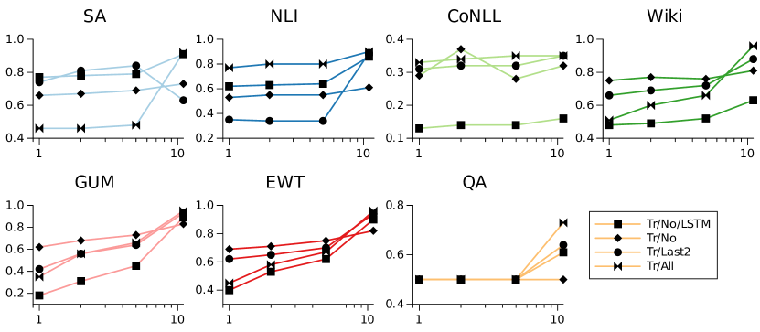
Figure 3: Comparison of BERT performances (macro $F_{1}$ score) per dataset with varying privacy budget $\varepsilon\in\{1,2,5,\infty\}$ on the $x$-axis (note the $\log$ scale).

While a performance drop is unsurprising with decreasing $\varepsilon$, there is no consistent pattern among tasks and models (see Fig. 3 in the Appendix). For instance, while the fully fine-tuned BERT model experiences a relatively large drop for sentiment analysis, its drop for NLI is almost negligible. The actual choice of the model should be therefore taken with a specific privacy requirement in mind.

5 Conclusion

We explored differentially-private training on seven NLP datasets. Based on a thorough analysis we formulate three take-home messages. (1) Skewed class distributions, which are inherent to many NLP tasks, hurt performance with DP-SGD, as the majority classes are often overrepresented in these models. (2) Fine-tuning and thus noisifying different transformer layers affects task-specific behavior so that no single approach generalizes over various tasks, unlike in a typical non-private setup. In other words, there is no one general setup in terms of fine-tuning to achieve the greatest performance for a differentially private model, considering multiple tasks. The best setting is task-specific. (3) Previous works have misinterpreted private NER due to an unsuitable evaluation metric, ignoring class imbalances in the dataset.

Appendix A Hyperparameter tuning

For each model, hyperparametertuning is conducted, and learning rates in the range of $0.1$ and $10^{-5}$ are tested. The batch size is set to 32 unless differential privacy and finetuning prohibit such a large size due to memory consumption. If this is the case, the batch size is reduced by a power of 2.
For the differentially private models, we obtain the best learning rate for $\varepsilon=1$ and use it for the same model type with $\varepsilon=2$ and $\varepsilon=5$.

Appendix B Privacy Settings

B.1 Chosen privacy settings

As the randomized response (section 3.2 in (Dwork and Roth, 2013)) is considered good privacy with $\varepsilon=\ln(3)\approx 1.1$, we conduct our experiments with $\varepsilon=1$. Moreover, as this work aims to understand the behavior of differential privacy, we additionally consider experiments with $\varepsilon=2$ and $\varepsilon=5$ to vary the degree of privacy applied to the model. Throughout all our experiments, we set $\delta$ to $10^{-5}$.

B.2 Obtaining the privacy parameters

To achieve a specific ($\varepsilon$,$\delta$)-differential privacy guarantee, one has to carefully add the right amount of noise to the gradient during every update step. Unfortunately, it is not possible to calculate the amount of noise needed to achieve a certain ($\varepsilon$,$\delta$)-differentially private model in closed-form for DP-SGD. However, the amount of noise only depends on the training dataset size, the number of maximum update steps, as well as $\delta$ and the noise multiplier. Knowing these parameters, one can estimate the resulting $\varepsilon$ value. Exploiting this ability, we iteratively test different sets of parameters and choose the ones that most closely resemble the desired $\varepsilon$.

To calculate the resulting $\varepsilon$ given the parameter set, we use Tensorflow Privacy. In order to incorporate the actual privacy component to the model, we use the Opacus library (Yousefpour et al., 2021), specifying the amount of noise we calculated for a given $\varepsilon$ value with Tensorflow Privacy.

Appendix C Efficiency and scalability of differentially private models

While the performance of a model is a crucial factor in its evaluation, one other aspect, especially when aiming to reduce energy consumption and development time, is gaining significance. Specifically, this is the time it takes for the model to optimize once across all batches and then evaluate itself against the evaluation dataset (epoch time).

A significant increase in epoch time is observed in all experiments when training in the differentially private setting. This increase is possibly related to the number of entries in the dataset. As shown in Table 3, larger datasets such as SNLI (570k entries) for NLI or SQuAD 2.0 (150k entries) for QA present a significantly larger increase in epoch time, compared to tasks trained on smaller datasets (such as IMDb for SA (50k entries), CoNLL’03 for NER (15k entries) or EWT for POS-tagging (13k entries)).

Another possible influence on the epoch time is number of fine-tuned parameters of the model. When adding further fine-tuning, the increase in epoch time tends to get larger. Throughout all tasks shown in Table 3, a larger difference is shown for the fully fine-tuned transformer (Tr/All), as when only fine-tuning the last two layers (Tr/Last2). However, future work further examining these possible correlations is necessary for providing a clearer picture.

Epoch time differences with and without differential privacy (DP)
Task	fine-tuned Layers of BERT base	epoch time without DP	epoch time with DP	difference
SA	Tr/Last2	4 min 22 sec	0 h 10 min 32 sec	0 h 06 min 10 sec
SA	Tr/All	9 min 07 sec	0 h 47 min 08 sec	0 h 38 min 01 sec
NER (CoNLL’03)	Tr/Last2	0 min 26 sec	0 h 02 min 24 sec	0 h 01 min 58 sec
NER (CoNLL’03)	Tr/All	0 min 57 sec	0 h 27 min 55 sec	0 h 26 min 58 sec
NLI	Tr/Last2	13 min 15 sec	3 h 37 min 15 sec	3 h 24 min 00 sec
NLI	Tr/All	22 min 32 sec	9 h 57 min 57 sec	9 h 35 min 25 sec
POS-tagging (EWT)	Tr/Last2	0 min 53 sec	0 h 06 min 12 sec	0 h 05 min 19 sec
POS-tagging (EWT)	Tr/All	1 min 12 sec	0 h 49 min 25 sec	0 h 48 min 13 sec
QA	Tr/Last2	12 min 21 sec	1 h 57 min 43 sec	1 h 45 min 22 sec
QA	Tr/All	44 min 07 sec	11 h 05 min 15 sec	10 h 21 min 08 sec

Table 3: Average epoch time during the training process for each task and two transformer fine-tuning settings (Tr/All and Tr/Last2). Right-most column shows the difference between the differentially private and non-private models.

Appendix D Analysis of the learning rate

For non-private models, using smaller learning rates usually leads to slower convergence towards a local minimum. This effect can be compensated when training for enough epochs. When considering a training process using differential privacy, this assumption no longer holds. One reason is that with every update step, random noise is added to the model, or in other words, no step is exactly towards the optimal direction. Thus, a smaller learning rate, or more necessary steps to reach a local optimum, increases the probability in moving in the wrong direction.

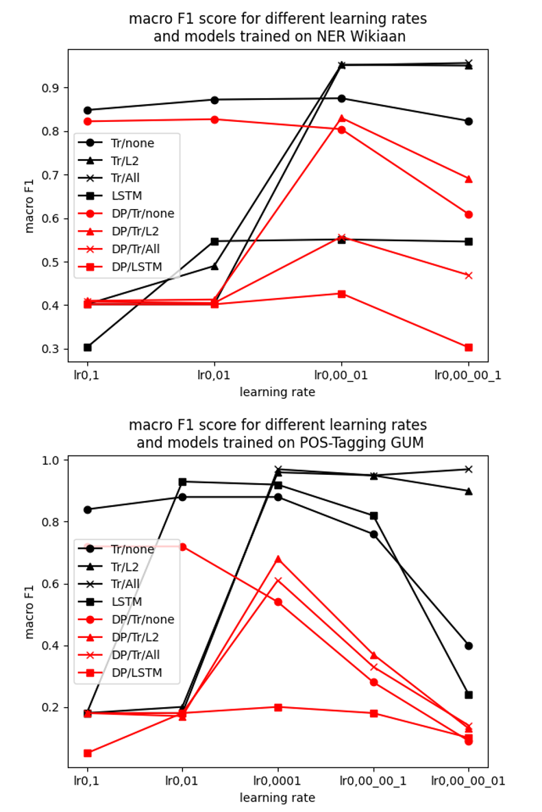
Figure 2: Both plots display the different macro $F_{1}$ scores for each model and the corresponding learning rate. It is notable, that for the differentially private models a smaller learning rate tends to (more quickly) result in worse performance.

This behavior can be observed in our experiments as well. When looking at Figure 2, the macro $F_{1}$ for the non-private experiments (black) usually increases or converges when decreasing the learning rate. However, when analyzing the experiments with DP (red) it is notable that with a smaller learning rate, the macro $F_{1}$ score decreases earlier than in the setting without DP.

Appendix E Analysing XtremeDistilTransformer Model

To compare our results and achieve a more robust analysis, we repeated our experiments using the same setup as before, and trained the XtremeDistilTransformer Model (XDTM) Mukherjee and Hassan Awadallah (2020).

E.1 Comparing both non-private models

When comparing the XDTM with BERT and no differential privacy, we achieve similar behavior. It is however notable, that for SA the XDTM/Last2 setup is much better than Tr/Last2. Similar results can be seen for NLI where only (Tr/No) presents better results compared to the BERT model. Furthermore, the XDTM trained on CoNLL fails to learn the task as it not only mistakes the I and B prefix, but also the tag itself. However, when training the XDTM on Wikiann, we can see much better performance. One reason could be the reduced tag size (9 for CoNLL and 7 for Wikiann). When looking at POS-tagging, we can see similar behavior for both GUM and EWT. Here the best choice is either the XDTM/No/LSTM or XDTM/All. Both XDTM/Last2 or XDTM/No show significantly lower performance. This behavior comes as a surprise, as the BERT model performs similarly in every setting. For QA, the non-private models are all less accurate except for XDTM with an additional LSTM.

E.2 Differentially Private XtremeDistilTransformer Model

When analyzing the different tasks and how the models behave when introduced to differential privacy, we can group them into two categories. While SA, NLI barely show a drop in macro $F_{1}$, NER on Wikiann as well as POS-tagging on GUM and EWT display a larger drop (Wikiann: between 14% and 4%, GUM: between 73% and 19%, EWT: between 66% and 19%). Additionally, as the non private model trained on CoNLL already had very low performance, it can be ignored in this analysis. We could not run QA experiments because of a limited access to further GPU compute capacity. For QA, the fully finetuned XDTM almost always predicts ‘unanswerable’. In contrast, the XDTM with an additional LSTM does predict spans. These predictions however, result in a worse performance of the model (about 0.33 $F_{1}$), compared to a model only predicting unanswerable (about 0.5 $F_{1}$).

E.3 Compare the differentially private setting to BERT

The main difference in differentially private SA between BERT and XDTM is that XDTM has no significant drop for all settings. Contrarily, BERT shows a large performance decline when fine-tuning all layers.

When training XDTM on NLI, it shows a better performance than the BERT model. This comes to a surprise, as one would expect XDTM to have a lower accuracy, since it was trained to mimic BERT’s behavior and has less parameters.

For NER with CoNLL, on the one hand both models show a bad macro $F_{1}$, where XDTM is about 15% worse than BERT. On the other hand, when training the two models on Wikiann, we can see that they are about the same if we include an LSTM after the (XtremeDistil) BERT layer. When omitting this extra network we can see a significant drop (about 40%) for XDTM.

For both POS-tagging tasks, XDTM is significantly worse than BERT, between 29% and 14% for GUM and 40% to 14% for EWT. For QA, the performance of the differentially-private XDTM is about the same as for BERT. However, the additional LSTM seems to be worse for the XDTM as for BERT. The reason is that XDTM predicts a lot of false spans. This is not the case for Tr/No/LSTM, as it only predicts ‘unanswerable’.

E.4 Conclusion for differential private XtremeDistilTransformer Model

To conclude, our experiments show that using XDTM for the tasks with differential privacy can be useful for simple classification tasks with small numbers of classes (such as SA or NLI). However, if the number of classes increase (such as NER or POS-tagging), differentially private XDTMs tend to perform worse than BERT. It is worth mentioning, however, that training differentially private XDTMs is much faster than using the full BERT model. See table 4 for the exact difference. Additionally, this speedup is also a direct result of larger possible batch sizes. This is made possible as the memory needed for these models is less than for the full BERT model.

Runtime differences between the BERT model and the XtremeDistilTransformer Model
Task	Finetuned Layers of BERT Model	BERT runtime without DP	XDTM runtime without DP	difference no DP	BERT runtime with DP	XDTM runtime with DP	difference DP
SA	last 2	4 min 22 sec	0 min 21 sec	4 min 01 sec	0 h 10 min 32 sec	0 min 21 sec	0 h 10 min 11 sec
SA	all	9 min 07 sec	0 min 52 sec	8 min 15 sec	0 h 47 min 08 sec	14 min 29 sec	0 h 32 min 39 sec
NER	last 2	0 min 26 sec	0 min 16 sec	0 min 10 sec	0 h 02 min 24 sec	0 min 17 sec	0 h 2 min 07 sec
NER	all	0 min 57 sec	0 min 25 sec	0 min 32 sec	0 h 27 min 55 sec	1 min 34 sec	0 h 26 min 21 sec
NLI	last 2	13 min 15 sec	2 min 34 sec	10 min 41 sec	3 h 37 min 15 sec	3 min 36 sec	3 h 33min 39 sec
NLI	all	22 min 32 sec	18 min 32 sec	4 min 00 sec	9 h 57 min 57 sec	62 min 32 sec	8 h 55 min 25 sec
EWT	last 2	0 min 53 sec	0 min 16 sec	0 min 37 sec	0 h 06 min 12 sec	0 min 15 sec	0 h 06 min 03 sec
EWT	all	1 min 12 sec	0 min 19 sec	0 min 53 sec	0 h 49 min 25 sec	1 min 32 sec	0 h 47 min 53 sec
QA	last 2	12 min 21 sec	6 min 45 sec	5 min 36 sec	1 h 57 min 43 sec	6 min 32 sec	1 h 51 min 11 sec
QA	all	44 min 07 sec	7 min 24 sec	36 min 43 sec	11 h 05 min 15 sec	53 min 35 sec	10 h 11 min 40 sec

Table 4: The difference in epoch time for the BERT and XDTM model; The time is the average epoch time during the training process. It can be seen, that the XDTM needs a lot less time to train. There are two main reasons for this expected behavior. (1) The XDTM is smaller, therefore, fewer parameters need to be trained. (2) The smaller model uses less memory, therefore, a larger batch size can be used.

Appendix F Detailed tables and figures

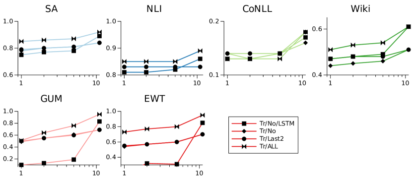
Figure 4: Comparison of XDTM performances (macro $F_{1}$ score) per dataset with varying privacy budget $\varepsilon\in\{1,2,5,\infty\}$ on the $x$-axis (note the $\log$ scale).

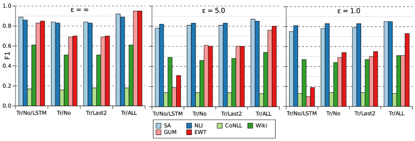
Figure 5: Macro $F_{1}$ scores for non-private ($\varepsilon=\infty$) and two private configurations ($\varepsilon\in\{5;1\}$) grouped by a particular model (x-axis) with XDTM as a base model.

$\downarrow$ gold	Neg	Pos
Neg	12497	3
Pos	12497	2

Table 5: Confusion matrix for the fully fine-tuned BERT model Tr/All with $\varepsilon=1$ on sentiment analysis.

$\downarrow$ gold	Neg	Pos
Neg	21137	3863
Pos	3162	21838

Table 6: Confusion matrix for Tr/None/LSTM with $\varepsilon=1$ on sentiment analysis.

	GUM		EWT
	Train	Test	Train	Test
NOUN	17,873	2,942	34,781	4,132
PUNCT	13,650	1,985	23,679	3,106
VERB	10,957	1,647	23,081	2,655
PRON	7,597	1,128	18,577	2,158
ADP	10,237	1,698	17,638	2,018
DET	8,334	1,347	16,285	1,896
PROPN	7,066	1,230	12,946	2,076
ADJ	6,974	1,116	12,477	1,693
AUX	4,791	719	12,343	1,495
ADV	4,180	602	10,548	1,225
CCONJ	3,247	587	6,707	739
PART	2,369	335	5,567	630
NUM	2,096	333	3,999	536
SCONJ	2,095	251	3,843	387
X	244	24	847	139
INTJ	392	87	688	120
SYM	156	35	599	92

Table 7: Distribution of all possible tags for POS-Tagging

	CoNLL’03		Wikiann
	Test	Train	Test	Train
O	38,554	170,524	42,879	85,665
I-LOC	1,919	1,157	6,661	13,664
B-PER	0	6,600	4,649	9,345
I-PER	2,773	4,528	7,721	15,085
I-ORG	2,491	3,704	11,825	23,668
I-MISC	909	1,155	–	–
B-MISC	9	3,438	–	–
B-LOC	6	7,140	5,023	10,081
B-ORG	5	6,321	4,974	9,910

Table 8: Distribution of all possible tags for NER

	CoNLL’03	Wikiann
O	0.98	0.86
I-LOC	0.00	0.46
B-PER	0.00	0.69
I-PER	0.67	0.57
I-ORG	0.01	0.54
I-MISC	0.00	–
B-MISC	0.00	–
B-LOC	0.00	0.44
B-ORG	0.00	0.14

Table 9: F1-scores per class for NER using the fully fine-tuned BERT Tr/All and $\varepsilon=1$. Except for the O tag (highlighted) and I-PER, no other class is predicted with sufficient performance on CoNLL.

	GUM	EWT
NOUN	0.66	0.62
PUNCT	0.85	0.87
VERB	0.64	0.72
PRON	0.65	0.72
ADP	0.73	0.80
DET	0.81	0.83
PROPN	0.17	0.16
ADJ	0.13	0.03
AUX	0.41	0.69
ADV	0.00	0.10
CCONJ	0.06	0.02
PART	0.00	0.00
NUM	0.00	0.00
SCONJ	0.00	0.00
X	0.00	0.00
INTJ	0.00	0.00
SYM	0.00	0.00

Table 10: F1-scores per class for POS-tagging using the fully fine-tuned BERT Tr/All and $\varepsilon=1$. Highlighted rows achieve usable performance.

$\downarrow$ gold	O	B-PER	I-PER	B-ORG	I-ORG	B-LOC	I-LOC	B-MISC	I-MISC
O	38207	26	3	47	41	19	9	66	80
B-PER	0	0	0	0	0	0	0	0	0
I-PER	17	1556	1150	23	10	15	1	1	0
B-ORG	0	0	0	0	5	0	0	0	0
I-ORG	42	27	3	1514	767	53	29	42	14
B-LOC	0	0	1	0	2	0	1	0	2
I-LOC	22	7	3	49	12	1558	232	30	5
B-MISC	0	0	0	0	0	0	0	4	5
I-MISC	51	9	3	32	9	23	4	594	183

Table 11: Confusion matrix for NER on CoNLL’03 for the fully fine-tuned BERT model. It can be seen (highlighted) that the model sometimes falsely predicts the position of the tag. Yet, the tag itself is mostly correctly classified.

$\downarrow$ gold	O	B-PER	I-PER	B-ORG	I-ORG	B-LOC	I-LOC	B-MISC	I-MISC
O	37540	61	38	149	0	304	0	0	0
B-PER	0	0	0	0	0	0	0	0	0
I-PER	33	1057	1521	77	0	48	0	0	0
B-ORG	0	0	0	4	0	1	0	0	0
I-ORG	192	90	142	1157	9	763	0	0	0
B-LOC	0	1	2	2	0	1	0	0	0
I-LOC	58	14	38	169	0	1577	0	0	0
B-MISC	1	2	0	1	0	5	0	0	0
I-MISC	178	21	14	110	0	502	0	0	0

Table 12: Confusion matrix for NER on CoNLL’03 for the fully fine-tuned BERT model with DP ($\varepsilon=1$). It can be seen (highlighted) that the model sometimes falsely predicts the type of tag. The positional error is still present.

$\downarrow$ gold	O	I-LOC	B-PER	I-PER	I-ORG	I-MISC	B-MISC	B-LOC	B-ORG
O	41021	52	9	6	9	32	4	4	5
I-LOC	1935	0	1	0	0	1	0	0	1
B-PER	0	0	0	0	0	0	0	0	0
I-PER	2821	2	1	0	0	3	0	0	0
I-ORG	2524	3	1	1	0	2	1	0	0
I-MISC	1013	1	0	0	0	1	0	0	0
B-MISC	9	0	0	0	0	0	0	0	0
B-LOC	6	0	0	0	0	0	0	0	0
B-ORG	5	0	0	0	0	0	0	0	0

Table 13: Confusion matrix for NER on CoNLL’03 for the BILSTM with DP ($\varepsilon=1$). It can be seen that this model only predicts the outside tag (highlighted).

$\downarrow$ gold	O	I-LOC	B-PER	I-PER	I-ORG	I-MISC	B-MISC	B-LOC	B-ORG
O	3464	3190	4161	21208	170	6035	722	1993	144
I-LOC	130	153	252	1032	11	243	29	84	2
B-PER	0	0	0	0	0	0	0	0	0
I-PER	234	226	348	1440	20	377	34	140	3
I-ORG	271	184	310	1161	9	430	39	115	8
I-MISC	76	73	100	561	4	132	17	49	3
B-MISC	1	0	1	4	0	0	0	3	0
B-LOC	0	1	1	4	0	0	0	0	0
B-ORG	2	0	0	2	0	0	0	1	0

Table 14: Confusion matrix for NER on CoNLL’03 for the BILSTM with DP ($\varepsilon=0.00837$). It can be seen that with this much privacy the model only randomly chooses tags (highlighted).

References

- Abadi et al. (2016) Martin Abadi, Andy Chu, Ian Goodfellow, H. Brendan McMahan, Ilya Mironov, Kunal Talwar, and Li Zhang. 2016. Deep Learning with Differential Privacy. In Proceedings of the 2016 ACM SIGSAC Conference on Computer and Communications Security, pages 308–318, Vienna, Austria. ACM.
- Bagdasaryan et al. (2019) Eugene Bagdasaryan, Omid Poursaeed, and Vitaly Shmatikov. 2019. Differential Privacy Has Disparate Impact on Model Accuracy. In Advances in Neural Information Processing Systems 32, pages 15479–15488, Vancouver, Canada. Curran Associates, Inc.
- Bowman et al. (2015) Samuel R. Bowman, Gabor Angeli, Christopher Potts, and Christopher D. Manning. 2015. A large annotated corpus for learning natural language inference. In Proceedings of the 2015 Conference on Empirical Methods in Natural Language Processing, pages 632–642, Lisbon, Portugal. Association for Computational Linguistics.
- Carlini et al. (2020) Nicholas Carlini, Florian Tramer, Eric Wallace, Matthew Jagielski, Ariel Herbert-Voss, Katherine Lee, Adam Roberts, Tom Brown, Dawn Song, Ulfar Erlingsson, Alina Oprea, and Colin Raffel. 2020. Extracting Training Data from Large Language Models. arXiv preprint.
- Dwork and Roth (2013) Cynthia Dwork and Aaron Roth. 2013. The Algorithmic Foundations of Differential Privacy. Foundations and Trends® in Theoretical Computer Science, 9(3-4):211–407.
- Fang et al. (2020) Yuwei Fang, Siqi Sun, Zhe Gan, Rohit Pillai, Shuohang Wang, and Jingjing Liu. 2020. Hierarchical Graph Network for Multi-hop Question Answering. In Proceedings of the 2020 Conference on Empirical Methods in Natural Language Processing (EMNLP), pages 8823–8838, Online. Association for Computational Linguistics.
- Farrand et al. (2020) Tom Farrand, Fatemehsadat Mireshghallah, Sahib Singh, and Andrew Trask. 2020. Neither Private Nor Fair: Impact of Data Imbalance on Utility and Fairness in Differential Privacy. In Proceedings of the 2020 Workshop on Privacy-Preserving Machine Learning in Practice, pages 15–19, Virtual conference. ACM.
- Gururangan et al. (2018) Suchin Gururangan, Swabha Swayamdipta, Omer Levy, Roy Schwartz, Samuel Bowman, and Noah A. Smith. 2018. Annotation Artifacts in Natural Language Inference Data. In Proceedings of the 2018 Conference of the North American Chapter of the Association for Computational Linguistics: Human Language Technologies, Volume 2 (Short Papers), pages 107–112, New Orleans, LA. Association for Computational Linguistics.
- Habernal (2021) Ivan Habernal. 2021. When differential privacy meets NLP: The devil is in the detail. In Proceedings of the 2021 Conference on Empirical Methods in Natural Language Processing, pages 1522–1528, Punta Cana, Dominican Republic. Association for Computational Linguistics.
- Habernal (2022) Ivan Habernal. 2022. How reparametrization trick broke differentially-private text representation learning. In Proceedings of the 60th Annual Meeting of the Association for Computational Linguistics (Volume 2: Short Papers), pages 771–777, Dublin, Ireland. Association for Computational Linguistics.
- Hoory et al. (2021) Shlomo Hoory, Amir Feder, Avichai Tendler, Sofia Erell, Alon Peled-Cohen, Itay Laish, Hootan Nakhost, Uri Stemmer, Ayelet Benjamini, Avinatan Hassidim, and Yossi Matias. 2021. Learning and Evaluating a Differentially Private Pre-trained Language Model. In Findings of the Association for Computational Linguistics: EMNLP 2021, pages 1178–1189, Punta Cana, Dominican Republic. Association for Computational Linguistics.
- Igamberdiev and Habernal (2022) Timour Igamberdiev and Ivan Habernal. 2022. Privacy-Preserving Graph Convolutional Networks for Text Classification. In Proceedings of the Language Resources and Evaluation Conference, pages 338–350, Marseille, France. European Language Resources Association.
- Jana and Biemann (2021) Abhik Jana and Chris Biemann. 2021. An Investigation towards Differentially Private Sequence Tagging in a Federated Framework. In Proceedings of the Third Workshop on Privacy in Natural Language Processing, pages 30–35, Online. Association for Computational Linguistics.
- Kerrigan et al. (2020) Gavin Kerrigan, Dylan Slack, and Jens Tuyls. 2020. Differentially Private Language Models Benefit from Public Pre-training. In Proceedings of the Second Workshop on Privacy in NLP, pages 39–45, Online. Association for Computational Linguistics.
- Maas et al. (2011) Andrew L. Maas, Raymond E. Daly, Peter T. Pham, Dan Huang, Andrew Y. Ng, and Christopher Potts. 2011. Learning Word Vectors for Sentiment Analysis. In Proceedings of the 49th Annual Meeting of the Association for Computational Linguistics: Human Language Technologies, pages 142–150, Portland, Oregon, USA. Association for Computational Linguistics.
- Madasu and Anvesh Rao (2019) Avinash Madasu and Vijjini Anvesh Rao. 2019. Sequential Learning of Convolutional Features for Effective Text Classification. In Proceedings of the 2019 Conference on Empirical Methods in Natural Language Processing and the 9th International Joint Conference on Natural Language Processing (EMNLP-IJCNLP), pages 5657–5666, Hong Kong, China. Association for Computational Linguistics.
- McMahan et al. (2018) H. Brendan McMahan, Daniel Ramage, Kunal Talwar, and Li Zhang. 2018. Learning Differentially Private Recurrent Language Models. In Proceedings of the 6th International Conference on Learning Representations, pages 1–14, Vancouver, BC, Canada.
- Mukherjee and Hassan Awadallah (2020) Subhabrata Mukherjee and Ahmed Hassan Awadallah. 2020. XtremeDistil: Multi-stage Distillation for Massive Multilingual Models. In Proceedings of the 58th Annual Meeting of the Association for Computational Linguistics, pages 2221–2234, Online. Association for Computational Linguistics.
- Pan et al. (2017) Xiaoman Pan, Boliang Zhang, Jonathan May, Joel Nothman, Kevin Knight, and Heng Ji. 2017. Cross-lingual Name Tagging and Linking for 282 Languages. In Proceedings of the 55th Annual Meeting of the Association for Computational Linguistics (Volume 1: Long Papers), pages 1946–1958, Vancouver, Canada. Association for Computational Linguistics.
- Rahimi et al. (2019) Afshin Rahimi, Yuan Li, and Trevor Cohn. 2019. Massively Multilingual Transfer for NER. In Proceedings of the 57th Annual Meeting of the Association for Computational Linguistics, pages 151–164, Florence, Italy. Association for Computational Linguistics.
- Rajpurkar et al. (2018) Pranav Rajpurkar, Robin Jia, and Percy Liang. 2018. Know What You Don’t Know: Unanswerable Questions for SQuAD. In Proceedings of the 56th Annual Meeting of the Association for Computational Linguistics (Volume 2: Short Papers), pages 784–789, Melbourne, Australia. Association for Computational Linguistics.
- Rogers et al. (2020) Anna Rogers, Olga Kovaleva, and Anna Rumshisky. 2020. A Primer in BERTology: What We Know About How BERT Works. Transactions of the Association for Computational Linguistics, 8:842–866.
- Silveira et al. (2014) Natalia Silveira, Timothy Dozat, Marie Catherine De Marneffe, Samuel R. Bowman, Miriam Connor, John Bauer, and Christopher D. Manning. 2014. A gold standard dependency corpus for English. In Proceedings of the Ninth International Conference on Language Resources and Evaluation (LREC’14), pages 2897–2904, Reykjavik, Iceland. European Language Resources Association (ELRA).
- Tjong Kim Sang and De Meulder (2003) Erik F. Tjong Kim Sang and Fien De Meulder. 2003. Introduction to the CoNLL-2003 Shared Task: Language-Independent Named Entity Recognition. In Proceedings of the Seventh Conference on Natural Language Learning at HLT-NAACL 2003, pages 142–147.
- Yousefpour et al. (2021) Ashkan Yousefpour, Igor Shilov, Alexandre Sablayrolles, Davide Testuggine, Karthik Prasad, Mani Malek, John Nguyen, Sayan Ghosh, Akash Bharadwaj, Jessica Zhao, Graham Cormode, and Ilya Mironov. 2021. Opacus: User-Friendly Differential Privacy Library in PyTorch. arXiv preprint.
- Zeldes (2017) Amir Zeldes. 2017. The GUM corpus: creating multilayer resources in the classroom. Language Resources and Evaluation, 51(3):581–612.