Neutrinoless double-beta decay: combining quantum Monte Carlo and the nuclear shell model with the generalized contact formalism

Abstract

We devise a framework based on the generalized contact formalism that combines the nuclear shell model and quantum Monte Carlo methods and compute the neutrinoless double-beta decay of experimentally relevant nuclei, including ⁷⁶Ge, ¹³⁰Te, and ¹³⁶Xe. In light nuclei, we validate our nuclear matrix element calculations by comparing against accurate variational Monte Carlo results. Due to additional correlations captured by quantum Monte Carlo and introduced within the generalized contact formalism, in heavier systems, we obtain long-range nuclear matrix elements that are about 30% smaller than previous shell-model results. We also evaluate the recently recognized short-range nuclear matrix element estimating its coupling by the charge-independence-breaking term of the Argonne $v_{18}$ potential used in the Monte Carlo calculations. Our results indicate an enhancement of the total nuclear matrix element by around 30%.

I Introduction

Neutrinoless double-beta decay ($0\nu\beta\beta$) is a hypothetical transition of atomic nuclei, forbidden by the Standard Model of particle physics, in which two neutrons are transmuted into two protons and two electrons are emitted with no accompanying antineutrinos Furry (1939). The measurement of $0\nu\beta\beta$ decay would have profound implications, demonstrating that lepton number is not a symmetry of nature, proving that the neutrino mass has a Majorana component Schechter and Valle (1982)—so that neutrinos and antineutrinos are the same particle—and, since two matter particles are created without the corresponding antimatter ones, illuminating the matter dominance in the universe. In addition, assuming the decay is mediated by the exchange of light neutrinos, it would provide invaluable insight on the neutrino mass scale and ordering Dell’Oro et al. (2016); Cardani (2019).

Because $0\nu\beta\beta$ is a second order decay, in practice it can only be detected in the few nuclei where $\beta$ decay is either energetically forbidden or strongly suppressed by spin change. Current best limits are given for ⁷⁶Ge ($T^{0\nu}_{1/2}>1.8\times 10^{26}$ yr Agostini et al. (2020)) and ¹³⁶Xe ($T^{0\nu}_{1/2}>1.07\times 10^{26}$ yr Gando et al. (2016)), and in this decade next-generation ton-scale experiments plan to reach $T^{0\nu}_{1/2}\sim 10^{28}$ yr, mainly in ⁷⁶Ge, ¹⁰⁰Mo, ¹³⁰Te or ¹³⁶Xe Kharusi et al. (2018); Adams et al. (2021); Abgrall et al. (2021); Armstrong et al. (2019). Since the decay involves physics beyond the Standard Model (BSM), its rate is proportional to a parameter describing the lepton number violation in that BSM mechanism. In addition, the decay rate is also governed by a nuclear matrix element (NME) that encodes the structure of the initial and final nuclei. Thus, extracting specific BSM information from half-life measurements demands reliable NMEs. This involves high-quality nuclear structure studies of heavy nuclei such as ⁷⁶Ge or ¹³⁶Xe. In this work we focus on the light Majorana neutrino exchange, but NMEs for other decay mechanisms can be calculated in the same fashion.

Most NME calculations use the quasiparticle random-phase approximation (QRPA) Mustonen and Engel (2013); Šimkovic et al. (2013); Hyvärinen and Suhonen (2015); Fang et al. (2015), nuclear shell model (SM) Menendez et al. (2009); Iwata et al. (2016); Horoi and Neacsu (2016); Coraggio et al. (2020), energy-density functional theory Rodriguez and Martinez-Pinedo (2010); López Vaquero et al. (2013); Yao et al. (2015); Yao and Engel (2016) or the interacting-boson model Barea et al. (2015); Deppisch et al. (2020). Besides other aspects—for an extensive review see Ref. Engel and Menéndez (2017)—these many-body methods show deficiencies related to the inconsistent treatment of the $0\nu\beta\beta$-decay operator. These may appear as missing nuclear correlations or two-nucleon currents in the decay operator. Ab initio many-body methods, in contrast, treat transition operators consistently, as they describe nuclear properties emerging from the bare interaction between protons and neutrons. This way they reproduce well $\beta$-decay rates in light- and medium-mass nuclei Gysbers et al. (2019); King et al. (2020) without any adjustments—usually known as “quenching”—, a feature required by less sophisticated many-body approaches like those mentioned above Chou et al. (1993); Wildenthal et al. (1983); Martínez-Pinedo et al. (1996); Pirinen and Suhonen (2015); Barea et al. (2015). Ab initio methods relying on single-particle basis expansion have calculated $0\nu\beta\beta$-decay NMEs for ⁴⁸Ca Novario et al. (2021); Yao et al. (2020); Wirth et al. (2021), or even heavier ⁷⁶Ge and ⁸²Se Belley et al. (2021). On the other hand, quantum Monte Carlo (QMC) approaches are very accurate, but so far limited to light nuclei with up to $A\leq 12$ nucleons Pastore et al. (2018a); Cirigliano et al. (2018). QMC treats accurately short-range nuclear dynamics, a key aspect for $0\nu\beta\beta$ transitions where decaying neutrons are typically a few fm apart. This is even more critical for the recently recognized short-range NME Cirigliano et al. (2018, 2019).

The generalized contact formalism (GCF) is a powerful tool to model the short-range behavior of nuclear distributions, both in coordinate and momentum space Weiss et al. (2015a, b, 2018); Cruz-Torres et al. (2021). Nuclear wave functions show a universal short-range behavior determined by the nuclear interaction; the only dependence on the specific nucleus comes about as an overall factor, proportional to the number of short-range correlated (SRC) pairs. Hence, the GCF is applicable across the nuclear chart, provided that these normalization factors are known. In this work, we use state-of-the-art variational Monte Carlo (VMC) and SM $0\nu\beta\beta$ transition densities to determine the ratios of normalization factors—which do not depend on the nuclear interaction—and correct the short-range part of the SM transition densities, assuming they describe well the long-range behavior. This way we include the short-range dynamics captured by the VMC into the SM. Although similar in spirit to correcting shell-model transition densities with Jastrow correlations Miller and Spencer (1976); Šimkovic et al. (2009); Benhar et al. (2014); Wang et al. (2019), our approach is more systematic, as it allows us to exactly match VMC results in $A\leq 12$ systems, and can accommodate a variety of nuclear interactions.

After validating our method in light nuclei where VMC calculations are available, we make NME predictions for nuclei used in $0\nu\beta\beta$ experiments, including ⁴⁸Ca, ⁷⁶Ge, ¹³⁰Te, and ¹³⁶Xe. Our results include estimates of the theoretical uncertainty associated with our method. In addition to the usual long-range NME, we compute the leading-order short-range NME, for which our approach may be particularly reliable. We follow recent analyses and estimate the coupling associated with this term by the charge-independence-breaking (CIB) term of the Argonne $v_{18}$ (AV18) potential used in the VMC calculations. While for this work we use the phenomenological AV18 plus the three-nucleon Urbana X (UX) force, our method is general and can readily be applied to interactions derived within chiral effective field theory.

The manuscript is organized as follows. First, we introduce the $0\nu\beta\beta$ transition potentials in Sec. II. Section III describes the many-body methods, while Sec. IV presents our NME results. Finally, Sec. V summarizes our main conclusions and future perspectives.

II $0\nu\beta\beta$ Transition potentials

Under the closure approximation Pantis and Vergados (1994); Faessler et al. (1991); Sen’kov et al. (2014), the $0\nu\beta\beta$ NME between the initial and final nuclear states $|\Psi_{i}\rangle$ and $|\Psi_{f}\rangle$ reads

$$M^{0\nu}=\langle\Psi_{f}|O^{0\nu}|\Psi_{i}\rangle\,.$$ (1)

We focus on the light Majorana neutrino exchange. For this mechanism the long-range transition operator can be cast as a sum of Fermi (F), Gamow-Teller (GT) and tensor (T) contributions $O^{0\nu}_{L}=O^{0\nu}_{F}+O^{0\nu}_{GT}+O^{0\nu}_{T}$, where

$$O^{0\nu}_{F} =(4\pi R_{A})\sum_{a\neq b}V^{0\nu}_{F}(r_{ab})\tau_{a}^{+}\tau_{b}^{+}\,,$$

$$O^{0\nu}_{GT} =(4\pi R_{A})\sum_{a\neq b}V^{0\nu}_{GT}(r_{ab})\,\sigma_{ab}\,\tau_{a}^{+}\tau_{b}^{+}\,,$$

$$O^{0\nu}_{T} =(4\pi R_{A})\sum_{a\neq b}V^{0\nu}_{T}(r_{ab})S_{ab}\,\tau_{a}^{+}\tau_{b}^{+}\,.$$ (2)

Here $\boldsymbol{\sigma}_{a}$ and $\tau_{a}$ represent nucleon spin and isospin operators, respectively, $\sigma_{ab}=\boldsymbol{\sigma}_{a}\cdot\boldsymbol{\sigma}_{b}$, and the tensor operator is $S_{ab}=3(\boldsymbol{\sigma}_{a}\cdot\hat{r}_{ab})(\boldsymbol{\sigma}_{b}\cdot\hat{r}_{ab})-\sigma_{ab}$ with $r_{ab}$ the internucleon distance. The nuclear radius $R_{A}=1.2\,A^{1/3}$ fm is inserted by convention to make the NME dimensionless. The coordinate-space neutrino potentials above are obtained from the standard Fourier transform:

$$V_{\alpha}^{0\nu}(r_{ab})=\frac{1}{g_{A}^{2}}\int\frac{d^{3}\mathbf{q}}{(2\pi)^{3}}e^{i\mathbf{q}\cdot\mathbf{r}_{ab}}V_{\alpha}^{0\nu}(\mathbf{q}^{2})\,,$$ (3)

where $\mathbf{q}$ is the momentum transfer, $\alpha$ indicates F, GT, and T, and we take $g_{A}=1.27$ for the axial-vector coupling.

Defining $V_{\alpha}^{0\nu}(\mathbf{q}^{2})=\frac{1}{\mathbf{q}^{2}}v_{\alpha}(\mathbf{q}^{2})$ the relevant functions can be given in terms of the nucleon isovector vector, axial, induced pseudoscalar and magnetic form factors Pastore et al. (2018a); Engel and Menéndez (2017):

$$v_{F}(\mathbf{q}^{2}) =-g_{V}^{2}(\mathbf{q}^{2})\,,$$

$$v_{GT}(\mathbf{q}^{2}) =g_{A}^{2}(\mathbf{q}^{2})+\frac{2}{3}\frac{\mathbf{q}^{2}}{2m_{N}}g_{A}(\mathbf{q}^{2})g_{P}(\mathbf{q}^{2})$$

$$+\frac{1}{3}\frac{\mathbf{q}^{4}}{4m_{N}^{2}}g_{P}^{2}(\mathbf{q}^{2})+\frac{2}{3}\frac{\mathbf{q}^{2}}{4m_{N}^{2}}g_{M}^{2}(\mathbf{q}^{2})\,,$$

$$v_{T}(\mathbf{q}^{2}) =-\frac{2}{3}\frac{\mathbf{q}^{2}}{2m_{N}}g_{A}(\mathbf{q}^{2})g_{P}(\mathbf{q}^{2})-\frac{1}{3}\frac{\mathbf{q}^{4}}{4m_{N}^{2}}g_{P}^{2}(\mathbf{q}^{2})$$

$$+\frac{1}{3}\frac{\mathbf{q}^{2}}{4m_{N}^{2}}g_{M}^{2}(\mathbf{q}^{2})\,,$$ (4)

where $m_{N}=938.9$ MeV is the nucleon mass. Consistent with the $0\nu\beta\beta$ literature, for the single-nucleon form factors we adopt the simple dipole parameterization:

$$g_{V}(\mathbf{q}^{2}) =\frac{g_{V}}{(1+\mathbf{q}^{2}/\Lambda_{V}^{2})^{2}}\,,$$

$$g_{M}(\mathbf{q}^{2}) =(1+\kappa_{1})g_{V}(\mathbf{q}^{2})\,,$$

$$g_{A}(\mathbf{q}^{2}) =\frac{g_{A}}{(1+\mathbf{q}^{2}/\Lambda_{A}^{2})^{2}}\,,$$

$$g_{P}(\mathbf{q}^{2}) =-\frac{2m_{N}}{q^{2}+m_{\pi}^{2}}g_{A}(\mathbf{q}^{2})\,,$$ (5)

with vector coupling $g_{V}=1$, anomalous nucleon isovector magnetic moment $\kappa_{1}=3.7$, and pion mass $m_{\pi}=138$ MeV. The cutoff values are $\Lambda_{V}=0.85$ GeV and $\Lambda_{A}=1.04$ GeV. More sophisticated functional forms for these form factors exist Ye et al. (2018), including some based on a systematic z-expansion Meyer et al. (2016). However, for the relatively small momentum transfer at play in $0\nu\beta\beta$ processes, $|\mathbf{q}|\sim 200$ MeV, no significant differences are expected with respect to the simple dipole ansatz.

Figure 1 displays the radial dependence of the transition potentials, and shows that the T component is clearly much smaller than both the F and GT ones. This behavior is reflected in the magnitude of the corresponding NMEs, as highlighted in a number of previous calculations Simkovic et al. (1999); Kortelainen and Suhonen (2007); Menendez et al. (2009). Including the form factors regularizes the potentials at short interparticle distances, while the typical $1/r_{ab}$ behavior at large $r_{ab}$ is preserved.

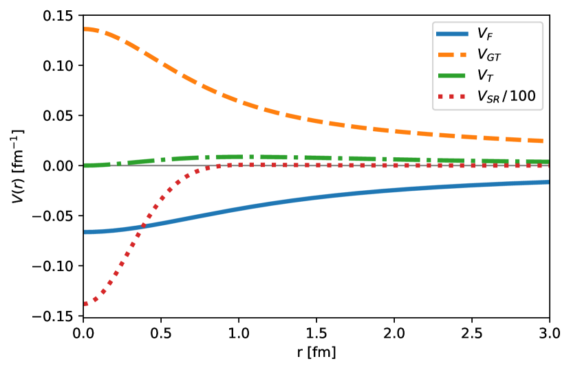
Figure 1: Fermi (solid blue curve), Gamow-Teller (dashed orange curve), tensor (dot-dashed green curve), and short-range (dot red curve) transition potentials.

The authors of Ref. Cirigliano et al. (2018) have demonstrated that an effective field theory approach of the light-neutrino exchange $0\nu\beta\beta$ decay requires a leading-order counter-term to absorb the divergences induced by the long-range neutrino potential and ensure renormalizability. This new short-range (SR) operator is associated with a Fermi spin structure and a SR neutrino potential:

$$O^{0\nu}_{S}=(4\pi R_{A})\sum_{a\neq b}V^{0\nu}_{S}(r_{ab})\tau_{a}^{+}\tau_{b}^{+}\,,$$ (6)

$$V_{S}^{0\nu}(r_{ab})=2\frac{g_{\nu}^{\text{NN}}}{g_{A}^{2}}\delta^{(3)}_{R}(\mathbf{r}_{ab})\,,$$ (7)

where $\delta^{(3)}_{R}(\mathbf{r}_{ab})$ is a regularized three-dimensional Dirac delta function. In contrast to Ref. Cirigliano et al. (2019), the above definition includes a factor $1/g_{A}^{2}$ so that the full light-Majorana transition operator is $O^{0\nu}=O^{0\nu}_{F}+O^{0\nu}_{GT}+O^{0\nu}_{T}+O^{0\nu}_{S}$. Consistent with the opposite sign in the definition of the F, GT and T contributions, the sign of the SR potential is also different to Ref. Cirigliano et al. (2019).

The value of the new coupling $g_{\nu}^{\text{NN}}$ arises from non-perturbative QCD dynamics and could in principle be found by matching to lattice-QCD calculations of light-neutrino exchange amplitudes Davoudi and Kadam (2021a, b). It can also be obtained by reproducing the synthetic $2n\rightarrow 2p+2e$ data provided by Refs. Cirigliano et al. (2021a, b). Alternatively, Ref. Cirigliano et al. (2019) notes that renormalizing the nucleon-nucleon ($N\!N$) scattering amplitude with Coulomb photon exchange also requires a short-range interaction with coupling $(C_{1}+C_{2})/2$, and connects $0\nu\beta\beta$ and CIB SR couplings: $g_{\nu}^{\text{NN}}=C_{1}$. Further, assuming the same value for the two couplings entering the CIB of $N\!N$ potentials, so that $g_{\nu}^{\text{NN}}\simeq(C_{1}+C_{2})/2$, describes well synthetic $2n\rightarrow 2p+2e$ data Cirigliano et al. (2021b). We follow this approach, which allows us to evaluate short range $0\nu\beta\beta$-decay NMEs for a variety of nuclei.

We compute the short-range behavior of nuclear states from the high-quality AV18 $N\!N$ potential. Hence, when evaluating NMEs we make the consistent replacement

$$g_{\nu}^{\text{NN}}\delta^{(3)}_{R}(\mathbf{r}_{ab})\to-\frac{6}{e^{2}}v_{S1}^{cd}(r_{ab})\,.$$ (8)

The full expression for the short-range component of the CIB term of AV18, $v_{S1}^{cd}(r_{ab})$, for the spin $S=0$, isospin $T=1$ channel can be found in Eq. (32) of Ref. Wiringa et al. (1995) and it is displayed in Fig. 1. To better gauge the importance of $V_{S}^{0\nu}$, we also consider the expression derived from the CIB contribution of the local, $\Delta$-full chiral effective field theory $N\!N$ potential of Ref. Piarulli et al. (2016). Specifically, for the NV-Ia^∗ model $(C_{1}+C_{2})/2=-1.03$ fm² and $\delta^{(3)}_{R}(\mathbf{r}_{ab})=e^{-r_{ab}^{2}/R_{S}^{2}}/(\pi^{3/2}R_{S}^{3})$ with $R_{S}=0.8$ fm.

Throughout this work, two-body transition densities play a crucial role

$$4\pi r^{2}\rho_{F}(r) =\langle\Psi_{f}|\sum_{a<b}\delta(r-r_{ab})\tau_{a}^{+}\tau_{b}^{+}|\Psi_{i}\rangle\,,$$

$$4\pi r^{2}\rho_{GT}(r) =\langle\Psi_{f}|\sum_{a<b}\delta(r-r_{ab})\sigma_{ab}\,\tau_{a}^{+}\tau_{b}^{+}|\Psi_{i}\rangle\,,$$

$$4\pi r^{2}\rho_{T}(r) =\langle\Psi_{f}|\sum_{a<b}\delta(r-r_{ab})S_{ab}\,\tau_{a}^{+}\tau_{b}^{+}|\Psi_{i}\rangle\,,$$ (9)

and $\rho_{S}(r)=\rho_{F}(r)$. All NMEs can be obtained integrating the above densities:

$$M^{0\nu}_{\alpha}=\int_{0}^{\infty}dr\,C^{0\nu}_{\alpha}(r)\,,$$ (10)

where we define $C^{0\nu}_{\alpha}(r)\equiv(8\pi R_{A})4\pi r^{2}\rho_{\alpha}(r)V^{0\nu}_{\alpha}(r)$ with the additional factor $2$ to compensate the restricted sum $a<b$ in Eq. (9).

III Many-body methods

III.1 Variational Monte Carlo

The VMC method solves the Schrödinger equation by approximating the true ground state of the system with a suitably parametrized variational wave function $\Psi_{T}$. The Rayleigh-Ritz variational principle

$$\frac{\langle\Psi_{T}|H|\Psi_{T}\rangle}{\langle\Psi_{T}|\Psi_{T}\rangle}=E_{T}\geq E_{0}$$ (11)

is exploited to find the optimal set of variational parameters. The VMC takes as input the Hamiltonian

$$H=\sum_{i}-\frac{\hbar^{2}}{2m}\,{\nabla}_{i}^{2}+\sum_{i<j}v_{ij}+\sum_{i<j<k}V_{ijk}\ ,$$ (12)

which consists of non-relativistic single-nucleon kinetic energy terms, and two- and three-nucleon interactions. As for the latter, in this work, we utilize the AV18 $N\!N$ interaction (Wiringa et al., 1995) in combination with the UX three-nucleon force. UX is intermediate between the Urbana and Illinois families of potentials Carlson et al. (2015), and is essentially a truncation of the Illinois-7 (IL7) model Pieper (2008); it has the form of Eq.(17) in Ref.Carlson et al. (2015), including two-pion S- and P-wave terms and a short-range isospin-independent repulsion, with the parameter values of IL7, but without the three-pion-ring term or short-range isospin dependence. The highly successful Green’s Function Monte Carlo calculations of light nuclei with AV18+IL7 shown in Ref.Carlson et al. (2015) start from VMC calculations with AV18+UX.

The VMC trial wave function is typically written as

$$|\Psi_{T}\rangle=\Big{(}1+\sum_{i<j<k}F_{ijk}\Big{)}\Big{(}\mathcal{S}\prod_{i<j}F_{ij}\Big{)}|\Phi_{J}\rangle\,,$$ (13)

where $F_{ij}$ and $F_{ijk}$ are two- and three-body correlation operators, respectively and $\mathcal{S}$ denotes a symmetrized product over nucleon pairs. The latter is required for the wave function to be antisymmetric, as, in general, the spin-isospin dependent correlation operators $F_{ij}$ do not commute.

To account for the alpha-cluster structure of light nuclei the anti-symmetric Jastrow wave function is constructed as a sum over independent-particle terms, $\Phi_{A}$, each having four nucleons in an $\alpha$-like core and the remaining $(A-4)$ nucleons in $p$-shell orbitals Pieper et al. (2002):

$$|\Phi_{J}\rangle =\mathcal{A}\Bigg{[}\prod_{i<j<k}f^{c}_{ijk}\prod_{i<j\leq 4}f_{ss}(r_{ij})\prod_{k\leq 4<l\leq A}f_{sp}(r_{kl})$$

$$\times\sum_{LS[n]}\bigg{(}\beta_{LS[n]}\prod_{4<l<m\leq A}f_{pp}^{[n]}(r_{lm})$$

$$\times|\Phi_{A}(LS[n]JJ_{z}T_{z})_{1234:5\dots A}\rangle\bigg{)}\Bigg{]}\,.$$ (14)

The operator $\mathcal{A}$ denotes an antisymmetric sum over all possible partitions of the $A$ particles into four $s$-shell and $(A-4)$ $p$-shell states. The independent-particle wave function $|\Phi_{A}(LS[n]JJ_{z}T_{z})_{1234:5\dots A}\rangle$ with the desired total angular momentum and projection $JJ_{z}$ values of a given nuclear state is obtained using orbital-spin $LS$ coupling, which is most efficient for nuclei with up to $A\leq 12$. It includes a product over single-particle functions $\phi^{LS}_{p}(R_{\alpha l})$ ($4<l\leq A$) which are $p$-wave solutions of a particle in an effective $\alpha$-$N$ potential with Woods-Saxon and Coulomb terms. The symbol $[n]$ is the Young pattern that indicates the spatial symmetry of the angular momentum coupling of the $p$-shell nucleons Pudliner et al. (1997). The pair correlation function for particles within the $s$-shell, $f_{ss}$, arises from the structure of the $\alpha$ particle. The $f_{sp}$ is similar to the $f_{ss}$ at short range, but it has a long-range tail that approaches unity at large distances, allowing the wave function to develop a cluster structure, i.e., the asymptotic binding is provided only by the $\phi^{LS}_{p}(R_{\alpha l})$. Finally, $f_{pp}$ is set to give the appropriate clustering outside the $\alpha$ core, while $f^{c}_{ijk}$ is the three-body central correlations induced by the $N\!N$ potential.

For the $A=6$ case the ⁶He wave function has two spatial symmetry components: ¹S₀[2] and ³P₀[11], which give a complete p-shell representation. Since ⁶Be is taken as the charge-symmetric mirror, the ⁶He $\rightarrow$ ⁶Be transition densities are large and have no nodal structure. For the $A=12$ case, a complete p-shell representation gives the ¹²Be wave function two spatial symmetry components: ¹S₀[422] and ³P₀[332], while ¹²C has three additional components, given in Table 1. The normalized amplitudes for each component in Table 1 indicate that the dominant states in the initial wave function are a very small part of the final wave function, making the ¹²Be $\rightarrow$ ¹²C transition densities much smaller than for $A=6$. They are further reduced by the presence of a node in the transition densities, required by the isospin orthogonality of the two wave functions.

	1S0[44]	3P0[431]	1S0[422]	5D0[422]	3P0[332]
12Be	-	-	0.983	-	0.186
12C	0.947	0.314	0.055	0.015	0.033

Table 1: Normalized amplitudes for different spatial symmetry components in the VMC wave functions for ¹²Be and ¹²C.

In an earlier comparison of VMC and SM calculations Wang et al. (2019) the VMC wave function for ¹²C included only the leading [44] and [431] components. While these are by far the dominant part of the final state wave function, the small [422] and [332] components included here have a much greater spatial overlap with the ¹²Be wave function, leading to a significant change, particularly at long range, in the transition densities. In particular, the GT NME with the more complete ¹²C wave function is about double that of the previous VMC calculation, while the F and T increase by 10-20%. This improves the agreement between VMC and the earlier SM calculations of Ref.Wang et al. (2019).

The expectation values of quantum mechanical operators of the form of Eq.(11) contain multi-dimensional integrals over all nucleon positions

$$\frac{\langle\Psi_{T}|\mathcal{O}|\Psi_{T}\rangle}{\langle\Psi_{T}|\Psi_{T}\rangle}=\frac{\int d\mathbf{R}\Psi^{\dagger}_{T}(\mathbf{R})\mathcal{O}\Psi_{T}(\mathbf{R})}{\int d\mathbf{R}\Psi^{\dagger}_{T}(\mathbf{R})\Psi_{T}(\mathbf{R})}\,,$$ (15)

and Metropolis-Hastings Monte Carlo techniques are employed to efficiently evaluate them. These Monte Carlo samples are also used to compute the two-body transition densities of Eq.(9) and to estimate their statistical uncertainties.

III.2 Nuclear Shell Model

The nuclear SM is one the most successful nuclear many-body methods to describe the properties of ground and excited states, including electromagnetic and weak transitions Brown and Wildenthal (1988); Caurier et al. (2005); Otsuka et al. (2020). It is also one of the common methods to compute $0\nu\beta\beta$-decay NMEs Menendez et al. (2009); Horoi and Neacsu (2016); Iwata et al. (2016); Coraggio et al. (2020).

In order to handle both light and heavy nuclei, the nuclear SM simplifies the many-body problem by restricting to a relatively small configuration space consisting of one or two harmonic oscillator shells. This excludes from the calculation the core—filled with nucleons—below and the high-energy orbitals—empty—above the configuration space, but their impact is captured by an effective interaction corresponding to the configuration space. The resulting many-body Schrödinger equation is

$$H_{\text{eff}}\,|\Psi_{\text{SM}}\rangle=E\,|\Psi_{\text{SM}}\rangle,$$ (16)

which we solve using the $J$-coupled code NATHAN Caurier et al. (2005). Even though ab initio approaches allow one to obtain effective interactions solely based on $N\!N$ and three-nucleon forces Stroberg et al. (2019), in this work we use high-quality interactions obtained from $N\!N$ potentials complemented with small phenomenological adjustments, mostly on the monopole part Caurier et al. (2005).

For light $A\leq 12$ nuclei we use the p- and sd-shell configuration space and the PSDMWK interaction Warburton et al. (1992); Warburton and Brown (1992) corrected for center-of-mass contamination. In heavier nuclei we use the same configuration space and SM interactions as in previous SM studies Menendez et al. (2009); Menéndez (2018): the pf-shell with the KB3G interaction for ⁴⁸Ca, the $1p_{3/2}$, $1p_{1/2}$, $0f_{5/2}$, $0g_{9/2}$ space with the GCN2850 interaction Menendez et al. (2009) for ⁷⁶Ge, and the $1d_{5/2}$, $2s_{1/2}$, $1d_{3/2}$, $0g_{7/2}$, $0h_{11/2}$ space with the GCN5082 interaction Menendez et al. (2009) for ¹³⁰Te and ¹³⁶Xe.

The SM wave functions from Eq. (16) directly provide energies and other observables not dependent on radial degrees of freedom. However, for $0\nu\beta\beta$ decay the spatial part is relevant as well, and usually a harmonic oscillator (HO) basis is used for single-particle states Menendez et al. (2009); Menéndez (2018). Here we follow the improved approach of Ref. Wang et al. (2019) and obtain our transition densities replacing the standard HO spatial single-particle states by Woods-Saxon (WS) ones, which reflect a more realistic long-range asymptotic behavior. We consider two kinds of WS potential: first, the standard parametrization from Suhonen (WSS) Suhonen (2007); second, the potential proposed by Ref. Wang et al. (2019) adjusted to the experimental neutron and proton separation energies and taking all orbitals in the configuration space as bound (WSW)—however, these conditions cannot be met for $A=6$ which we only study with WSS. We have checked that alternative WS parametrizations Schwierz et al. (2007) give very similar results to WSS.

In light nuclei, Ref. Wang et al. (2019) shows that SM results with WSW orbitals greatly improve the agreement with VMC ones. The improvement with WSS is similar. However, extending the SM results with WS single-particle orbitals to heavy nuclei is challenging, and only HO calculations are currently feasible. Fortunately, we have tested in $A=48$ that the differences between using HO and WS orbitals become smaller for heavier systems. Figure 2 shows minor differences between the F transition density computed employing the two different parametrizations of the WS orbitals and the HO one for single-particle orbitals. Likewise, the GT and T transition densities are also very similar.

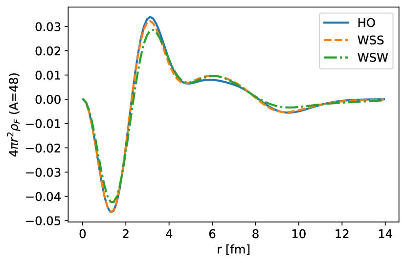
Figure 2: Fermi transition density for $A=48$ using the SM with HO, WSS, and WSW single-particle orbitals. 

Since the nuclear SM deals with regularized effective interactions, part of the short-range dynamics is missing in the wave functions. This shortcoming is common to other non ab initio approaches such as the QRPA, energy-density functional theory and interacting boson model. Because the short-range dynamics can impact $0\nu\beta\beta$ decay NMEs, typically calculations correct for missing SRCs via a Jastrow-type function. Different parametrizations have been provided by Miller-Spencer Miller and Spencer (1976) or based on Argonne and CD-Bonn potentials Šimkovic et al. (2009), or by others Cruz-Torres et al. (2018); Benhar et al. (2014); Roth et al. (2005). However, in this work we do not include any additional correlations of this kind, as we introduce the correct short-range dynamics captured by the VMC calculations using the GCF.

III.3 Generalized Contact Formalism

The GCF is an effective theory for describing the impact of SRCs on a variety of nuclear distributions and observables. This formalism has proven extremely successful in modeling the short-range and high-momentum parts of different nuclear densities Weiss et al. (2015b, 2018); Cruz-Torres et al. (2021), and also large momentum transfer electron scattering experiments sensitive to SRCs Weiss et al. (2019a); Schmidt et al. (2020); Pybus et al. (2020); Duer et al. (2019); Weiss et al. (2021) and other reactions Weiss et al. (2015a, 2016a, 2016b, 2019b). In a high-resolution picture, when two or more particles are close to each other, and, therefore, strongly interacting, the SM solution for the wave function—based on a regularized potential—becomes inaccurate Hen et al. (2013). For example, SRCs lead to a significant occupation of high momentum states absent in the SM. On the other hand, QMC methods fully capture these features but are limited to light nuclei. Therefore, the GCF provides an ideal framework to quantitatively incorporate the correct short-range behavior into shell-model calculations of heavy nuclei.

The GCF is based on scale separation, leading to wave-function factorization when two particles are very close to each other. Explicitly, any nuclear wave function $\Psi(\boldsymbol{r}_{1},\boldsymbol{r}_{2},...,\boldsymbol{r}_{A})$ is expected to obey the asymptotic form Weiss et al. (2015b)

$$\Psi\xrightarrow[r_{ij}\rightarrow 0]{}\sum_{\alpha}\varphi^{\alpha}(\boldsymbol{r}_{ij})A^{\alpha}(\boldsymbol{R}_{ij},\{\boldsymbol{r}_{k}\}_{k\neq i,j}).$$ (17)

Here $\boldsymbol{r}_{ij}=\boldsymbol{r}_{j}-\boldsymbol{r}_{i}$ and $\boldsymbol{R}_{ij}=(\boldsymbol{r}_{i}+\boldsymbol{r}_{j})/2$ are the relative and center of mass coordinates of the pair, and $\alpha$ denotes its quantum numbers, i.e., parity $\pi_{\alpha}$, spin $s_{\alpha}$, total angular momentum $j_{\alpha}$, and projection $j_{\alpha z}$, and total isospin $t_{\alpha}$ and projection $t_{\alpha z}$. Isospin quantum numbers are relevant to keep the nuclear wave function $\Psi$ anti-symmetric under permutations of any two nucleons. This convention is equivalent to the one in most previous GCF studies considering wave functions anti-symmetric under separate permutations of protons and neutrons. The solution of the zero-energy two-body Schrödinger equation $\varphi^{\alpha}(\boldsymbol{r}_{ij})$ describes the pair dynamics when the two nucleons are close together. It is a universal function, i.e. identical for all nuclei and all quantum states, but depends on the model and the nuclear interaction. It can be written as

$$\varphi^{\alpha}\left(\boldsymbol{r}\right)\equiv\eta_{t_{\alpha},t_{\alpha z}}\sum_{\ell_{\alpha}\in\pi_{\alpha}}\phi^{\alpha}(r)\left[Y_{\ell_{\alpha}}\left(\hat{\boldsymbol{r}}\right)\otimes\chi_{s_{\alpha}}\right]^{j_{\alpha}m_{\alpha}}\;,$$ (18)

where $\eta_{t,t_{z}}$ is the isospin function, $Y_{lm}$ spherical harmonics, $\chi_{sm}$ the two-body spin function, and the sum runs over orbital angular momenta $\ell_{\alpha}$ of correct parity $\pi_{\alpha}$ that can couple with $s_{\alpha}$ yielding $j_{\alpha}$. The radial dependence is modeled by $\phi^{\alpha}(r)$, which is independent of $j_{\alpha z}$ and, to good accuracy, also of $t_{\alpha z}$ due to isospin symmetry.

Based on this asymptotic form, the nuclear contacts for a nucleus with $A$ nucleons are defined as

$$C^{\alpha\beta}=\frac{A(A-1)}{2}\langle A^{\alpha}|A^{\beta}\rangle.$$ (19)

The factor $A(A-1)/2$ appears in place of the number of proton-proton, neutron-proton or neutron-neutron pairs present in previous publications because here the wave function is anti-symmetric under permutation of any two nucleons.

The diagonal contacts $C^{\alpha\alpha}$ are proportional to the number of correlated pairs in the nucleus with quantum numbers $\alpha$. However, in this work we apply the GCF to describe the short-range behavior of the two-body densities relevant for $0\nu\beta\beta$ transitions. Hence, we define new contact parameters that involve different initial ($i$) and final ($f$) nuclear states as

$$C^{\alpha\beta}(f,i)=\frac{A(A-1)}{2}\langle A^{\alpha}(f)|A^{\beta}(i)\rangle.$$ (20)

Using the above definition, we can write the dominant contributions to the transition densities defined in Eq. (9) at short distances. For F and GT transitions, we expect pairs in an s-wave state, mainly with $s=0$, $j=0$, $t=1$. Denoting the corresponding contact parameter for a transition of two neutrons to two protons ($nn\rightarrow pp$) with such quantum numbers as $C_{pp,nn}^{0}(f,i)$, the F transition density can be expressed as

$$\rho_{F}(r)\xrightarrow[r\rightarrow 0]{}\frac{1}{4\pi}|\phi^{0}(r)|^{2}C_{pp,nn}^{0}(f,i),$$ (21)

where $\phi^{0}(r)$ is the radial function for the $\ell=0$, $s=0$, $j=0$, $t=1$ channel. Since $\rho_{S}=\rho_{F}$, the above asymptotic form is valid for transition density associated with the short-range operator of Eq. (7). As for the GT transition, the $\sigma_{ab}$ operator leads to a factor of $(-3)$ in this $s=0$ channel and we similarly obtain

$$\rho_{GT}(r)\xrightarrow[r\rightarrow 0]{}-\frac{3}{4\pi}|\phi^{0}(r)|^{2}C_{pp,nn}^{0}(f,i),$$ (22)

which implies the following relation between the F and GT densities for short distances

$$\rho_{GT}(r\lesssim 1\;\textrm{fm})=-3\rho_{F}(r\lesssim 1\;\textrm{fm}).$$ (23)

Based on our previous experience with two-body densities Weiss et al. (2018); Cruz-Torres et al. (2021), these expressions should provide a good description of the transition densities for $r\lesssim 1$ fm.

To calculate the $0\nu\beta\beta$ matrix elements, we wish to combine the GCF expressions, valid at short distances, and the long-range behavior of the nuclear SM many-body wave functions. The main unknowns in this approach are the values of the relevant contacts, which in general depend upon the nucleus and on the particular nuclear interaction. Nevertheless, previous studies have shown that for the case of the contacts defined in Eq. (19), contact ratios $C^{\alpha\alpha}(X)/C^{\alpha\alpha}(Y)$, for any two nuclei $X$ and $Y$, are model independent Cruz-Torres et al. (2021); Weiss et al. (2019b); Tropiano et al. (2021). In this sense, contact ratios can be interpreted as long-range, low-resolution quantities that do not depend on the details of the nuclear interaction.

Such a model independence is expected to hold also for ratios of the contacts defined in Eq. (20). Therefore, the ratio of the contacts $C^{0,\text{SM}}_{pp,nn}(f_{1},i_{1})/C^{0,\text{SM}}_{pp,nn}(f_{2},i_{2})$—indices $1$ and $2$ denote different $0\nu\beta\beta$ decays—is inferred from SM transition densities at short distances. Then, the contact $C^{0,V_{N}}_{pp,nn}(f_{2},i_{2})$ is obtained by fitting the short-range behavior to the transition density “$2$” computed with VMC for a given realistic nuclear interaction $V_{N}$. Finally, the contact for transition “1” is obtained exploiting the model independence of the ratios:

$$C^{0,V_{N}}_{pp,nn}(f_{1},i_{1})=\frac{C^{0,\text{SM}}_{pp,nn}(f_{1},i_{1})}{C^{0,\text{SM}}_{pp,nn}(f_{2},i_{2})}C^{0,V_{N}}_{pp,nn}(f_{2},i_{2}).$$ (24)

This procedure allows us to obtain contact values of heavy nuclei for any nuclear interaction, using only a single ab-initio calculation for light nuclei and SM ones for both heavy and light nuclei. In Sec. IV we provide ample evidence on the accuracy of the model independence of contact ratios.

The contact value $C^{0,V_{N}}_{pp,nn}(f_{1},i_{1})$ and the corresponding short-range radial function fully determine the short-range part ($r\lesssim 1$ fm) of the transition densities for a given nuclear interaction. On the other hand, the SM is expected to provide high-quality transition densities at long distances. Thus, we merge the GCF and SM results continuously, by scaling the SM transition densities to match the GCF expression around $r\simeq 1$ fm. This approach, dubbed GCF-SM, allows us to obtain the F and GT transition densities for any given nuclear interaction—including heavy nuclei where direct ab initio calculations with high-resolution potentials are currently not possible. We integrate the resulting transition densities as in Eq. (10) to evaluate the relevant $0\nu\beta\beta$ NMEs.

In the case of the T transitions the leading contribution is expected to come from p-wave channels. There are three such channels (with $j=0,1,2$) which complicates the analysis. In addition, comparing SM and VMC calculations, it seems that the model-independence of the ratios does not hold for the T case. For this reason, in this work we estimate the T matrix element by the SM results with a $50\%$ uncertainty. This should not have a big impact on the total NME as the T part is expected to be small compared to the GT contribution Menendez et al. (2009); Engel and Menéndez (2017).

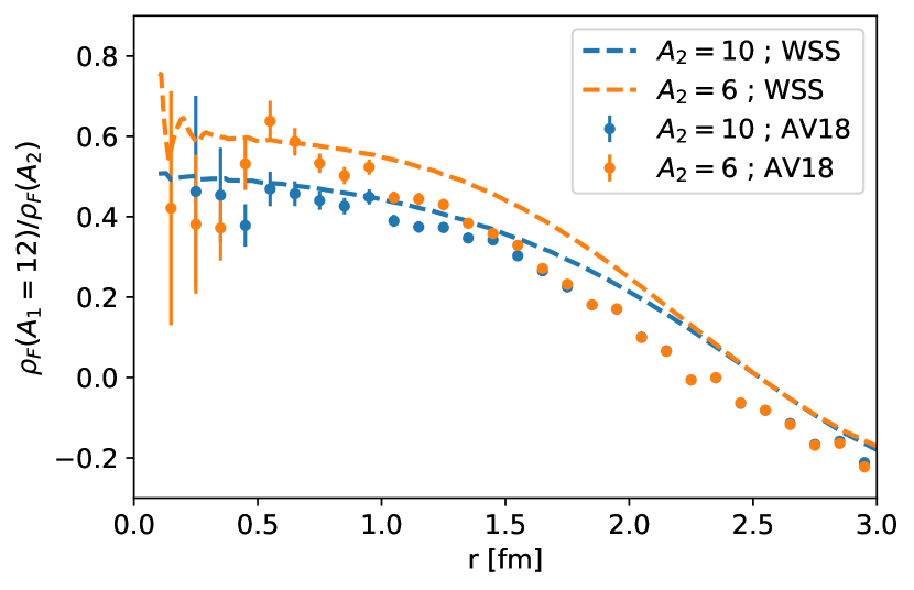
Figure 3: Fermi transition density ratio for different nuclei, calculated using different interactions (AV18 and SM). At short distances, the ratio plateaus and is similar for the two interaction models. 

IV Results and discussion

IV.1 Light nuclei

In order to use the GCF to describe the short-range part of the transition densities, we evaluate the contact $C_{pp,nn}^{0}(f,i)$ assuming the model independence of contact ratios. In light nuclei, the availability of both VMC and SM $0\nu\beta\beta$ transition densities allows us to test the accuracy of this approach. Figure 3 displays two ratios of F transition densities: ${}^{12}\textrm{Be}\to\,^{12}\textrm{C}$ decay over ${}^{10}\textrm{Be}\to\,^{10}\textrm{C}$ and over ${}^{6}\textrm{He}\to\,^{6}\textrm{Be}$, obtained with both the VMC and SM. At short distances the ratio reaches a plateau, as expected according to Eq. (21), representing the contact ratio of the two transitions. In addition, in both cases (e.g. $A=10$ and $A=6$) the value of the ratio at short distances is very similar for the VMC and SM calculations, indicating model independence.

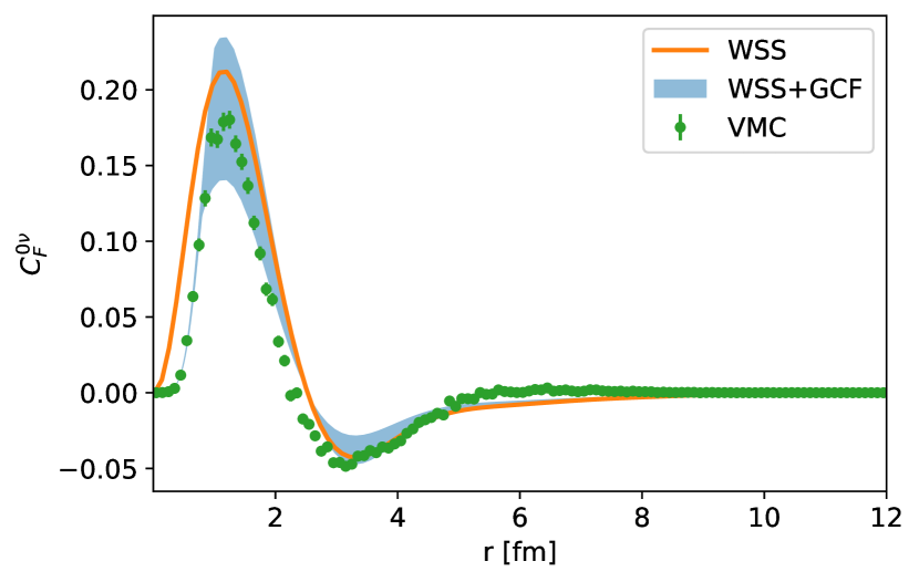
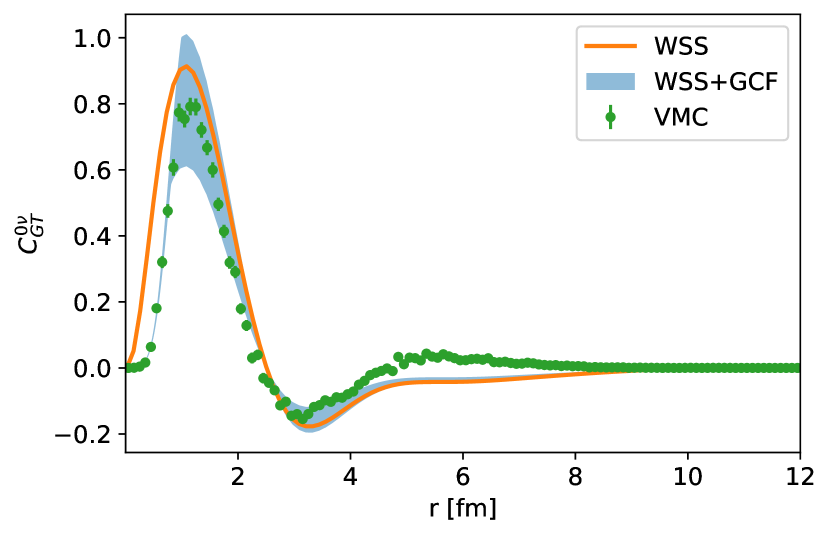
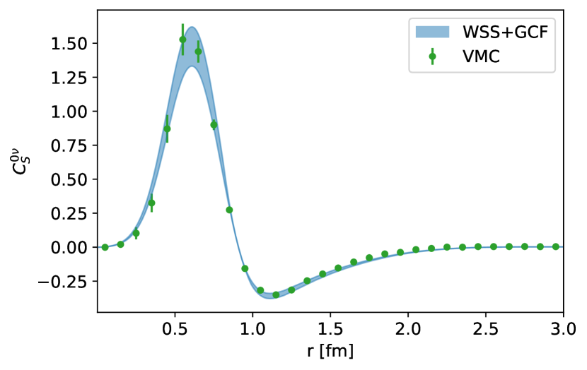
Figure 4: Fermi, Gamow-Teller and short-range transition densities calculated with the SM WSS (orange line), VMC (green points), and the combination of the GCF and SM WSS (blue band) approaches. For the latter, only VMC calculations for $A=6$ and $A=10$ are used to extract the ${}^{12}\textrm{Be}\rightarrow^{12}\textrm{C}$ contact value. 

To gauge the accuracy of our approach, we use the VMC transitions for $A=6$ and $A=10$ to predict results for $A=12$. The contact $\textrm{C}_{pp,nn}^{0}(^{10}\textrm{Be},^{10}\textrm{C})$ is fitted to the VMC calculations using the functional form of Eq. (21). We then obtain the $A=12$ contact $\textrm{C}_{pp,nn}^{0}(^{12}\textrm{Be},^{12}\textrm{C})$, based on the model independence of Eq. (24), multiplying $\textrm{C}_{pp,nn}^{0}(^{10}\textrm{Be},^{10}\textrm{C})$ by the average value of the SM ratio $\rho_{F}(A=12)/\rho_{F}(A=10)$ at short distances. We repeat the same procedure using as input the VMC transition densities for $A=6$. Comparing the two approaches yields $\lesssim 10\%$ differences in the extracted contact values, and we take the average as our best estimate for $\textrm{C}_{pp,nn}^{0}(^{12}\textrm{Be},^{12}\textrm{C})$, associated with a $10\%$ uncertainty.

Once the value of the contact is determined, we construct the short-range part of the F, GT and SR transition densities with Eqs. (21) and (22). We highlight the consistency of the approach, as the value of the contact is extracted from VMC calculations using the AV18+UX Hamiltonian, and the two-body function $\phi^{0}(r)$ is consistently computed with the AV18 $N\!N$ force.

For long distances we use the SM transition densities, after re-scaling them so that they are continuously merged with the short-range part. This part is expected to be well described by the SM, given the very good description it gives of nuclear structure and spectroscopy Caurier et al. (2005); Otsuka et al. (2020). In particular, long-range correlations have been studied extensively in $0\nu\beta\beta$ studies Hinohara and Engel (2014); Menéndez et al. (2014); Yao et al. (2021a), and the SM has proven to capture well important correlations such as those related to high-seniority components Caurier et al. (2008) or proton-neutron pairing Menéndez et al. (2016). Therefore, we expect that the GCF-SM describes also well the long-range part of the transition densities.

The upper, middle, and lower panels of Fig. 4 display the F, GT and SR transition densities obtained with the above procedure. The band is obtained by randomly varying separately the contact value within its $10\%$ uncertainty, and the matching point of GCF and SM between $0.8-1.0$ fm. Figure 4 shows an overall good agreement between the GCF-SM and the VMC results. In particular, our new method greatly improves upon the short-range behavior of the SM transitions densities, bringing them in excellent agreement with the VMC ones. It has to be noted that while introducing ad-hoc Jastrow-like correlations into SM calculations certainly ameliorates their short-range behavior, the agreement with ab-initio results is not as good Wang et al. (2019). In addition, the GCF can readily accommodate different interactions and correct SM calculations in a consistent fashion. The long range part of the transitions ($r\gtrsim 1$ fm), taken from the SM, also agrees well with the VMC. In this regard, an important role is played by the complete p-shell representation of the VMC ¹²C wave function utilized in this work, in contrast to earlier VMC calculations Pastore et al. (2018a); Cirigliano et al. (2019) that only included the leading [44] and [431] components. As expected, the transition density of the SR operator is almost perfectly described by our approach, at both short and long distances.

We further gauge the accuracy of the GCF-SM method by using either both the $A=10$ and $A=12$, or the $A=6$ and $A=12$ VMC transition densities, to predict $A=6$, or $A=10$ NMEs $M_{\alpha}^{0\nu}$, respectively, using Eq. (10). Figure 5 compares the GFC-SM the $A=6$, $A=10$, and $A=12$ F (upper panel) GT (middle panel) and SR (lower panel) NMEs for these nuclei to the VMC and standard SM results—see Table 2 for their numerical values. The VMC and GCF-SM matrix elements are consistent within error bars—little dependence on the particular WS parametrization is observed—and SR NMEs agree especially well. The SR SM values without correcting for SRC, not shown in Fig. 5, are about 10 times larger than the VMC ones, due to the scale of the AV18 SR potential, see Fig. 1. In almost all cases, complementing SM calculations with the GCF improves over the SM results. Perhaps more importantly, while uncertainties of the SM calculations are difficult to estimate, the GCF-SM error estimates appear to be robust.

We note that using SR transition potential from the NV-Ia* interaction changes the value of $M_{S}^{0\nu}$ by less than $20\%$, despite the differences in the shape of the transition densities $C_{S}^{0\nu}(r)$ are more dramatic. Nonetheless, fully consistent calculations of SR operators for potentials other than AV18 require using the appropriate two body function $\phi^{0}(r)$ and the corresponding VMC transition densities. This is left for future work.

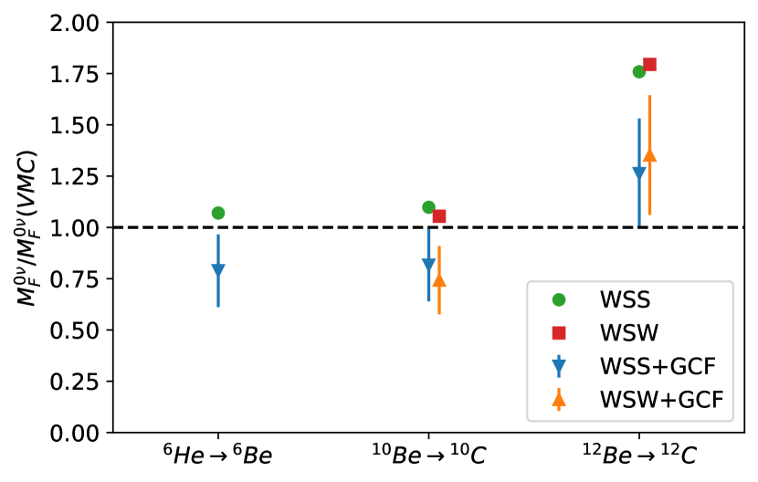
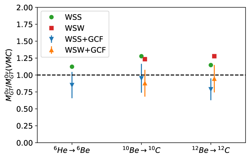
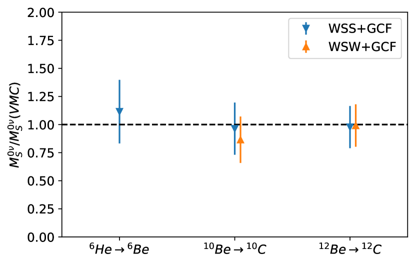
Figure 5: Ratio of nuclear matrix elements of the F (upper panel), GT (central panel), and SR (lower panel) operators. Results obtained combining the GCF and SM, or just the SM approach, divided by the VMC ones with the AV18+UX Hamiltonian. Both WSS and WSW parametrizations are used for the SM calculations.  

Transition	Method	F	GT	SR
6He $\rightarrow$ 6Be	VMC	0.935	3.706	0.296
	WSS	1.001	4.160	3.286
	WSS+GCF	0.74(17)	3.16(72)	0.33(8)
10Be $\rightarrow$ 10C	VMC	1.182	3.647	0.513
	WSW	1.246	4.500	4.457
	WSS	1.297	4.660	4.721
	WSW+GCF	0.88(20)	3.20(72)	0.44(11)
	WSS+GCF	0.96(21)	3.47(78)	0.49(12)
12Be $\rightarrow$ 12C	VMC2	0.102	0.365	0.347
	VMC5	0.113	0.757	0.348
	WSW	0.203	0.968	2.531
	WSS	0.199	0.868	2.562
	WSW+GCF	0.15(3)	0.72(15)	0.35(7)
	WSS+GCF	0.14(3)	0.60(12)	0.34(7)

Table 2: Fermi, Gamow-Teller, and short-range NMEs for the ⁶He $\rightarrow$ ⁶Be, ¹⁰Be$\rightarrow^{10}$C and ¹²Be $\rightarrow$ ¹²C transitions calculated using different methods. VMC₂ stands for VMC calculations with 2 components for ¹²C, while VMC₅ includes 5 components. The latter is used to extract the contact ratios.

IV.2 Heavy nuclei

Having validated the accuracy of the GCF-SM approach on light nuclei, we now turn our analysis to nuclei relevant to the $0\nu\beta\beta$ decay experimental program, currently beyond the reach of the VMC method. We obtain GCF-SM predictions of $0\nu\beta\beta$ transitions analogously to light nuclei, the only difference being that we use all the VMC and SM transition densities for $A=6$, $A=10$, and $A=12$ nuclei to extract the contact values. The short-range components of the transition densities are modeled according to Eqs. (21) and (22) and continuously matched to re-scaled SM results, so that the long-range part $C^{0\nu}_{\alpha}(r)$ is fully specified.

While for light nuclei $A\leq 12$ WSS and WSW clearly improve the transition densities in Eq. (9) in relation with the VMC results, the HO and WS radial wave functions lead to very similar results in ⁴⁸Ca, see Fig. 2. Based on this observation, for $A\geq 48$ nuclei our SM transitions are obtained with HO orbitals. On the other hand the SM transition densities for $A=6$, $A=10$, and $A=12$ used to extract the contact ratios against AV18+UX VMC results are always carried out with WS single-particle states. Specifically, we denote the HO results for heavy nuclei “HO(S)” or “HO(W)” depending on whether the WSS or WSW parametrization is used to extract the contacts from light-nuclei transitions.

Figure 6 illustrates the differences between SM and GCF-SM transition densities for the ${}^{76}\textrm{Ge}\rightarrow\,^{76}\textrm{Se}$ decay, covering the F, GT, and SR operators. The short-range behavior of the SM is modified in a consistent fashion as in light nuclei, and reflects the underlying realistic nuclear potential. Analogously to Fig. 5, we do not report the SM transition densities for the SR operator, as the corresponding NMEs are about 7 times larger than the GCF-SM values.

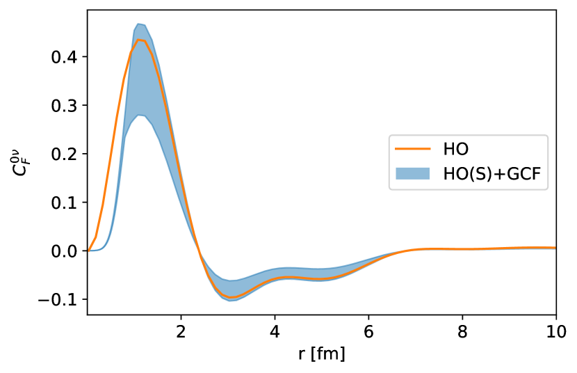
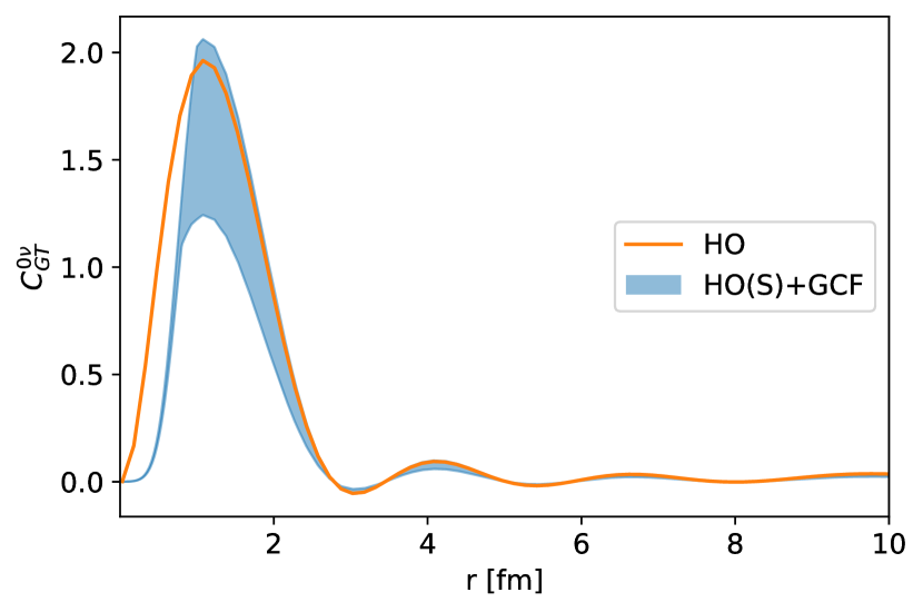
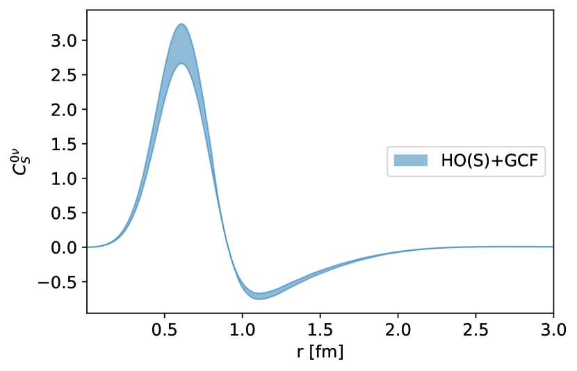
Figure 6: Transition densities $C_{F}^{0\nu}$ (upper panel), $C_{F}^{0\nu}$ (middle panel), and $C_{S}^{0\nu}$ (lower panel) for the ${}^{76}\textrm{Ge}\rightarrow^{76}\textrm{Se}$ decay obtained with the SM with HO orbitals (orange line) and the GCF-SM (blue band).

The GCF-SM results for the F, GT and SR matrix elements for $A=48$, $A=76$, $A=130$ and $A=136$ are displayed in Fig. 7 and their numerical values are listed in Table 3. We supplement these predictions with conservative estimates for the uncertainties associated to the matching procedure and the extraction of the contact ratios as described in Sec IV.1. Our results indicate that the F and GT matrix elements are reduced by about $20\%-45\%$ compared to the conventional SM calculations due to the additional SRC introduced via the GCF.

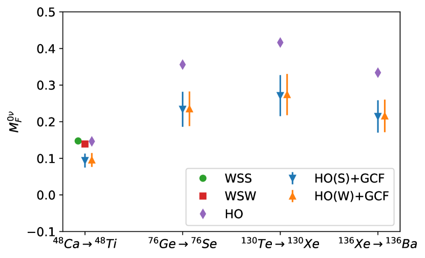
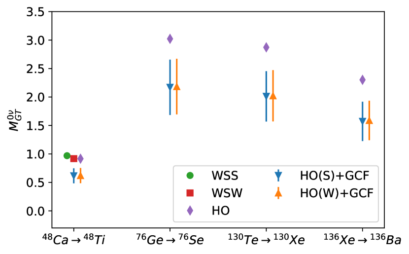
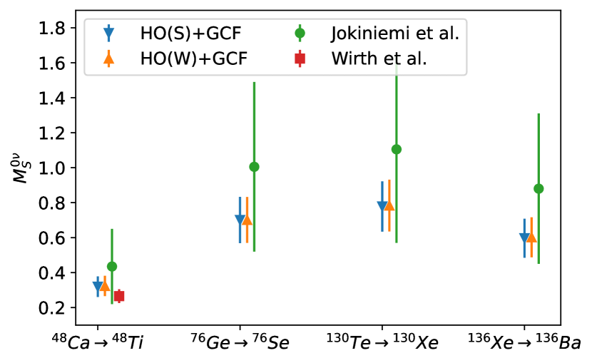
Figure 7: NMEs of the F (upper panel), GT (middle panel), and SR (lower panel) operators using the GCF-SM and the SM approaches,  compared to the SR results of Jokiniemi et al. Jokiniemi et al. (2021) and Wirth et al. Wirth et al. (2021). 

The bottom panel of Fig. 7 shows that the value of the short-range NME is significantly smaller in $A=48$ than in heavier nuclei, a trend which is similar when we replace the SR transition potential with the one corresponding to the NV-Ia* interaction—$M_{S}^{0\nu}$ only changes by about $20\%$. Figure 7 also indicates that our short-range NMEs are in general smaller but consistent within error-bars with the SM results by Jokiniemi et al. Jokiniemi et al. (2021), which cover a wider range of SR transition potentials—not including the AV18 one we use—and are further corrected by the SRC parametrization of Ref. Šimkovic et al. (2009). In contrast, we only use one SR potential and just include uncertainties associated to the matching procedure and the extraction of the contact ratios. The $M_{S}^{0\nu}$ values obtained with the QRPA by Jokiniemi et al. are somewhat larger than ours. Remarkably, our SR NME for ⁴⁸Ca is in good agreement with the in-medium similarity renormalization group (IMSRG) combined with the generator coordinate method (IM-GCM) ab-initio result of Wirth et al. Wirth et al. (2021). This is particularly interesting since they use a different nuclear interaction and also a different procedure for determining the SR coupling $g^{\text{NN}}_{\nu}$.

Transition	Method	F	GT	SR
48Ca $\rightarrow$ 48Ti	WSS	0.147	0.969	2.360
	WSW	0.139	0.917	2.043
	HO	0.146	0.916	2.356
	WSS+GCF	0.09(2)	0.66(14)	0.32(6)
	WSW+GCF	0.09(2)	0.62(13)	0.27(5)
	HO(S)+GCF	0.09(2)	0.62(13)	0.32(6)
	HO(W)+GCF	0.10(2)	0.62(13)	0.32(6)
76Ge $\rightarrow$ 76Se	HO	0.356	3.022	5.247
	HO(S)+GCF	0.23(5)	2.17(49)	0.70(13)
	HO(W)+GCF	0.24(5)	2.18(49)	0.70(13)
130Te $\rightarrow$ 130Xe	HO	0.416	2.873	5.804
	HO(S)+GCF	0.27(6)	2.01(44)	0.78(14)
	HO(W)+GCF	0.27(6)	2.02(45)	0.78(15)
136Xe $\rightarrow$ 136Ba	HO	0.334	2.302	4.564
	HO(S)+GCF	0.21(4)	1.57(35)	0.60(11)
	HO(W)+GCF	0.22(4)	1.59(35)	0.60(11)

Table 3: Fermi, Gamow-Teller, and short-range NMEs for the ⁴⁸Ca $\rightarrow$ ⁴⁸Ti, ⁷⁶Ge $\rightarrow$ ⁷⁶Se, ¹³⁰Te $\rightarrow$ ¹³⁰Xe and ¹³⁶Xe $\rightarrow$ ¹³⁶Ba transitions using the SM (HO, WSS, WSW) and the GCF-SM with different WS orbitals to fix the values of the contact ratios.

Eventually, the total $0\nu\beta\beta$ decay NME is the sum of the long-range term $M_{L}^{0\nu}=M_{GT}^{0\nu}+M_{F}^{0\nu}+M_{T}^{0\nu}$ and the short-range matrix element $M_{S}^{0\nu}$. As discussed in Section III, we evaluate the relatively small $M_{T}$ contribution within the standard SM, associated to a conservative $50\%$ uncertainty. Figure 8 presents our results for $M_{L}^{0\nu}$, highlighting that the GCF-SM reduces the value of $M_{L}^{0\nu}$ by about $15\%-40\%$ compared to the original SM calculations. Therefore, our approach introduces a much larger SRC effect than the one from typical SRC parametrizations such as the one from Ref. Šimkovic et al. (2009) used in SM $0\nu\beta\beta$ studies, see the very small difference between the SM (HO) and Jokiniemi et al. results from Ref. Jokiniemi et al. (2021). Figure 8 also compares our NMEs with the ab-initio results of Novario et al. Novario et al. (2021) using the Coupled Cluster (CC) method and of Yao et al. Yao et al. (2020) using the IM-GCM approach for ⁴⁸Ca and of Belley et al. Belley et al. (2021) using the valence space IMSRG (VS-IMSRG) method for ⁴⁸Ca and ⁷⁶Ge. Our long-range NMEs are in very good agreement with all the ab initio results for ⁴⁸Ca even though these calculations use different nuclear interactions, and are also consistent with the VS-IMSRG for ⁷⁶Ge. This good agreement supports our predictions for ¹³⁰Te and ¹³⁶Xe, for which ab initio NMEs are not available.

Comparing Figs. 7 and 8, it is apparent that the SR term contributes significantly to the total NME: $M_{S}^{0\nu}$ is around $35\%-60\%$ of $M_{L}^{0\nu}$ for $A=48$—in good agreement with Ref. Wirth et al. (2021)—and around $25\%-40\%$ for the heavier nuclei. Since $M_{S}^{0\nu}$ has the same sign as $M_{L}^{0\nu}$, the total matrix element would be enhanced, also in agreement with Ref. Wirth et al. (2021). Despite the differences between our results and the SM ones of Jokiniemi et al., the relative importance of the SR term is overall similar, while the QRPA predicts somewhat larger larger ratio values Jokiniemi et al. (2021).

It is important to highlight the differences between the GCF-SM and previous attemps to include SRCs into the SM and other approaches based on regularized interactions. Some of the correlation functions that produce larger effect of SRCs, e.g. those by Miller and Spencer Miller and Spencer (1976), were criticized because they lead to violation of isospin symmetry: the integral $\int_{0}^{\infty}r^{2}\rho_{F}(r)dr\neq 0$ when the isospin of the initial and final state is different Engel et al. (2011). Given the relatively large effects of SRCs, one might think that the GCF-SM approach can suffer from the same shortcomings. Ref. Engel et al. (2011) also claims that, in order to respect isospin symmetry, correlation functions should peak around $r\simeq 1$ fm with a value above 1 to compensate for the reduction of probability at short distances. This behavior eventually leads to a relatively small effect on the NME values. In contrast, to match the VMC and SM results an appropriate correlation function should be defined as the ratio of the corresponding transition densities—by construction, multiplying the SM results by this correlation function reproduces the VMC one. By comparing the VMC and SM transition densities presented in Fig. 4, we notice that the correlation function does not peak around $r\simeq 1$ fm. Furthermore, the GCF-SM approach has a significant difference in that the SM results are re-scaled to match the short-range behavior, so that the effect of the GCF does not approach unity at long distances unlike most SRC parametrizations. This re-scaling allows the GCF-SM to compensate for the short-range reduction without a peak at $r\simeq 1$ fm. Some violation of the isospin orthogonality can still be found in our actual results, but this is due to subleading corrections, like three-body correlations, and possible small differences between the SM and the exact solution at long distances. Eventually, the good agreement between the GCF-SM and VMC results in light nuclei shown in Fig. 4 demonstrates the accuracy of our method.

In addition, most of the available SRC functions assume in their derivation a simple form for the uncorrelated wave function, like a Slater determinant in Ref. Šimkovic et al. (2009). The latter differs from the SM wave function and therefore leads to inconsistencies when combined with SM calculations. Likewise, the correlation function based on VMC calculations introduced in Ref. Cruz-Torres et al. (2018) also uses a simple function for the uncorrelated part. Further, Ref. Cruz-Torres et al. (2018) uses proton-proton VMC densities of a given nucleus in contrast to the transition densities involving the initial and final nuclei used in the GCF-SM approach. In short, the GCF-SM replaces the need of introducing SRC functions by directly providing the appropriate short-range structure for any given $N\!N$ interaction.

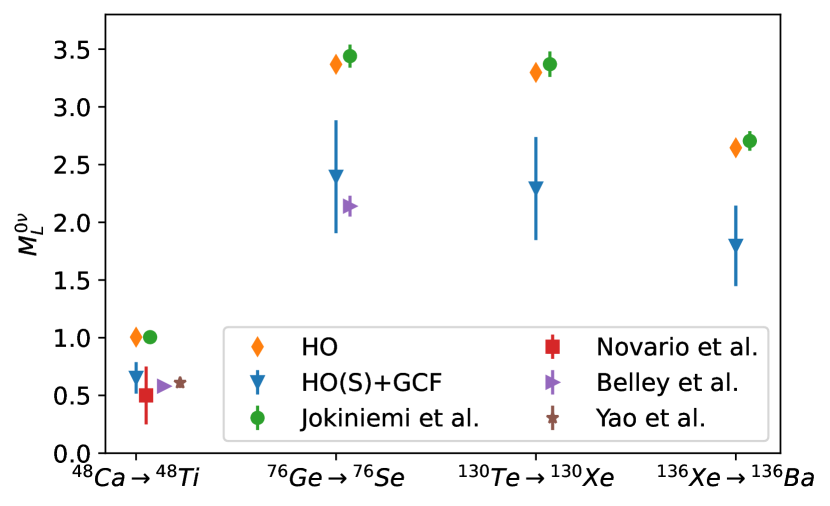
Figure 8: Long-range matrix element $M_{L}^{0\nu}$ calculated with the combination of the GCF and the SM (blue), the SM without (orange) and with SRCs from Jokiniemi et al. (green) Jokiniemi et al. (2021), the CC from Novario et al. (red) Novario et al. (2021), the VS-IMSRG from Belley et al. (purple) Belley et al. (2021), and the IMSRG+GCM from Yao et al. (brown) Yao et al. (2020). 

V Conclusions

We have introduced a novel protocol based on the GCF that combines SM and QMC methods to compute $0\nu\beta\beta$ decay nuclear matrix elements of heavy nuclei relevant for experimental searches. The GCF is used to describe the transition densities at short-distances from QMC calculations, while re-scaled SM calculations are used to model the long-range components. A key role in our GCF-SM approach is played by the “contact” values, which determine the number of short-range correlated pairs participating in the transition densities. Assuming their model-independence—extensively verified in diagonal two-body densities—we extract the contact values of heavy nuclei combining VMC calculations of light nuclei with SM transitions of both light and heavy isotopes. We verify the accuracy of this procedure on VMC transition densities of $A=6$, $A=10$, and $A=12$ nuclei. The latter are also improved compared to earlier calculations by introducing a complete p-shell representation of the ¹²Be wave function. We supplement the GCF-SM predictions by conservative estimates of the uncertainties due to the matching procedure and extracting the contact ratios.

We employ the GCF-SM to predict NMEs for ⁴⁸Ca, ⁷⁶Ge, ¹³⁰Te and ¹³⁶Xe. The long-range matrix elements are appreciably reduced by $15\%-40\%$ with respect to the SM calculations. In particular, the impact of SRCs is significantly larger within the GCF-SM than when using relatively-soft functions to incorporate SRCs effects into the SM. In fact, our approach replaces altogether the need of using correlation functions, since, besides an overall normalization factor, the short-range behavior of the transition density is fully determined by the GCF. Remarkably, our results are consistent within error bars with recent ab-initio results for ⁴⁸Ca and ⁷⁶Ge, carried out within the CC, and VS-IMSRG, and IM-GCM methods. Further, we make GCF-SM predictions for the heaviest emitters used in $0\nu\beta\beta$ searches: ¹³⁰Te and ¹³⁶Xe, for which ab-initio results are not currently available. Given the agreement with the VMC in the light-nuclei sector and with other ab-initio approaches for ⁴⁸Ca and ⁷⁶Ge, we believe that the GCF-SM is a reliable complementary approach to calculate $0\nu\beta\beta$ NMEs and reduce their theoretical uncertainty.

The GCF-SM method is especially suitable for calculating the recently introduced leading order SR matrix element. Using a transition potential consistent with the AV18 interaction used to compute the transition densities at short distances, we find that the SR term enhances the total NME by $25\%-40\%$ in heavy nuclei, which is consistent with IM-GCM and SM estimations. Nonetheless, our SR NMEs obtained based on the CIB of AV18 may need to be rescaled once the correct $g^{\text{NN}}_{\nu}$ coupling is determined—see Ref. Cirigliano et al. (2021a) for a recently proposed strategy using synthetic data.

A limitation of this work is the absence of two-body currents in the $0\nu\beta\beta$ decay, which are related to a consistent treatment of the transition operator. Two-body currents are necessary to reproduce $\beta$ decay matrix elements Pastore et al. (2018b); Gysbers et al. (2019), but are not fully included in any $0\nu\beta\beta$ calculation yet, where their impact has only been estimated within a simple approximation Menendez et al. (2011); Engel et al. (2014). However, Refs. Pastore et al. (2018b); Gysbers et al. (2019) indicate that two-body currents are relatively less important when using hard nuclear interactions characterized by high-momentum components, like AV18. In this sense, our NMEs the absence of two-body currents in our results may have a smaller impact than on the ab initio methods relying on single-particle basis expansion that deal with softer nuclear potentials.

The GCF-SM $0\nu\beta\beta$ matrix elements presented in this work rely on VMC calculations carried out with the AV18+UX Hamiltonian, and the short-range GCF two-body function has consistently been computed with AV18. In future work we plan to study the NME dependence on the nuclear Hamiltonian of choice, including those derived within chiral effective field theory. For instance, the local chiral Norfolk two- and three-body potentials can be readily incorporated in the GCF-SM method once the VMC calculations are carried out. On the other hand, including non-local potentials would require calculating transition densities for light nuclei with suitable many-body methods, like the no-core shell model Basili et al. (2020); Yao et al. (2021b).

A further development of the method is to improve the treatment of the T matrix element. This is especially important in view of a recent ab-initio studies that find relatively large T contributions compared to the SM Belley et al. (2021). This development will require disentangling the different p-wave contributions at short distances and additional analyses of the model independence of contact ratios.

More generally, the GCF-SM approach, anchored on VMC calculations of light nuclei, can be applied to incorporating the effect of SRCs in a variety of nuclear quantities accessible by the nuclear SM. We envision computing the transition densities relevant for studying the role of correlations and two-body currents in single-$\beta$ decay rates. As noted in Ref. King et al. (2020), the two-body densities exhibit a universal, i.e. nucleus independent, behavior at short distance. Also, we plan on utilizing the GCF-SM method to analyze momentum distributions and spectral functions of nuclei of interest in the context of electron-scattering experiments and for the accelerator-based neutrino oscillation program.

VI Acknowledgement

The present research is supported by the U.S. Department of Energy, Office of Science, Office of Nuclear Physics, under contract DE-AC02-06CH11357, the NUCLEI SciDAC program (A.L., R.B.W.), by the Laboratory Directed Research and Development program of Los Alamos National Laboratory under project number 20210763PRD1 (R.W.) and by the “Ramón y Cajal” program with grant RYC-2017-22781, and grants CEX2019-000918-M and PID2020-118758GB-I00 funded by MCIN/AEI/10.13039/501100011033 and, as appropriate, by ”ESF Investing in your future” (P.S. and J.M.). The work of A.L. is also supported by the DOE Early Career Research Program award. Quantum Monte Carlo calculations were performed on the parallel computers of the Laboratory Computing Resource Center, Argonne National Laboratory, the computers of the Argonne Leadership Computing Facility via the INCITE grant “Ab-initio nuclear structure and nuclear reactions”, and the 2020/2021 ALCC grant “Chiral Nuclear Interactions from Nuclei to Nucleonic Matter”.

References

- Furry (1939) W. H. Furry, Phys. Rev. 56, 1184 (1939).
- Schechter and Valle (1982) J. Schechter and J. W. F. Valle, Phys. Rev. D 25, 2951 (1982).
- Dell’Oro et al. (2016) S. Dell’Oro, S. Marcocci, M. Viel, and F. Vissani, Adv. High Energy Phys. 2016, 2162659 (2016), arXiv:1601.07512 [hep-ph] .
- Cardani (2019) L. Cardani, SciPost Phys. Proc. 1, 024 (2019), arXiv:1810.12828 [nucl-ex] .
- Agostini et al. (2020) M. Agostini et al. (GERDA), Phys. Rev. Lett. 125, 252502 (2020), arXiv:2009.06079 [nucl-ex] .
- Gando et al. (2016) A. Gando et al. (KamLAND-Zen), Phys. Rev. Lett. 117, 082503 (2016), [Addendum: Phys.Rev.Lett. 117, 109903 (2016)], arXiv:1605.02889 [hep-ex] .
- Kharusi et al. (2018) S. A. Kharusi et al. (nEXO), (2018), arXiv:1805.11142 [physics.ins-det] .
- Adams et al. (2021) C. Adams et al. (NEXT), JHEP 2021, 164 (2021), arXiv:2005.06467 [physics.ins-det] .
- Abgrall et al. (2021) N. Abgrall et al. (LEGEND), (2021), arXiv:2107.11462 [physics.ins-det] .
- Armstrong et al. (2019) W. R. Armstrong et al. (CUPID), (2019), arXiv:1907.09376 [physics.ins-det] .
- Mustonen and Engel (2013) M. T. Mustonen and J. Engel, Phys. Rev. C 87, 064302 (2013), arXiv:1301.6997 [nucl-th] .
- Šimkovic et al. (2013) F. Šimkovic, V. Rodin, A. Faessler, and P. Vogel, Phys. Rev. C 87, 045501 (2013), arXiv:1302.1509 [nucl-th] .
- Hyvärinen and Suhonen (2015) J. Hyvärinen and J. Suhonen, Phys. Rev. C 91, 024613 (2015).
- Fang et al. (2015) D.-L. Fang, A. Faessler, and F. Simkovic, Phys. Rev. C 92, 044301 (2015), arXiv:1508.02097 [nucl-th] .
- Menendez et al. (2009) J. Menendez, A. Poves, E. Caurier, and F. Nowacki, Nucl. Phys. A 818, 139 (2009), arXiv:0801.3760 [nucl-th] .
- Iwata et al. (2016) Y. Iwata, N. Shimizu, T. Otsuka, Y. Utsuno, J. Menéndez, M. Honma, and T. Abe, Phys. Rev. Lett. 116, 112502 (2016), [Erratum: Phys.Rev.Lett. 117, 179902 (2016)], arXiv:1602.07822 [nucl-th] .
- Horoi and Neacsu (2016) M. Horoi and A. Neacsu, Phys. Rev. C 93, 024308 (2016), arXiv:1511.03711 [nucl-th] .
- Coraggio et al. (2020) L. Coraggio, A. Gargano, N. Itaco, R. Mancino, and F. Nowacki, Phys. Rev. C 101, 044315 (2020), arXiv:2001.00890 [nucl-th] .
- Rodriguez and Martinez-Pinedo (2010) T. R. Rodriguez and G. Martinez-Pinedo, Phys. Rev. Lett. 105, 252503 (2010), arXiv:1008.5260 [nucl-th] .
- López Vaquero et al. (2013) N. López Vaquero, T. R. Rodríguez, and J. L. Egido, Phys. Rev. Lett. 111, 142501 (2013), arXiv:1401.0650 [nucl-th] .
- Yao et al. (2015) J. M. Yao, L. S. Song, K. Hagino, P. Ring, and J. Meng, Phys. Rev. C 91, 024316 (2015), arXiv:1410.6326 [nucl-th] .
- Yao and Engel (2016) J. M. Yao and J. Engel, Phys. Rev. C 94, 014306 (2016), arXiv:1604.06297 [nucl-th] .
- Barea et al. (2015) J. Barea, J. Kotila, and F. Iachello, Phys. Rev. C 91, 034304 (2015), arXiv:1506.08530 [nucl-th] .
- Deppisch et al. (2020) F. F. Deppisch, L. Graf, F. Iachello, and J. Kotila, Phys. Rev. D 102, 095016 (2020), arXiv:2009.10119 [hep-ph] .
- Engel and Menéndez (2017) J. Engel and J. Menéndez, Rept. Prog. Phys. 80, 046301 (2017), arXiv:1610.06548 [nucl-th] .
- Gysbers et al. (2019) P. Gysbers et al., Nature Phys. 15, 428 (2019), arXiv:1903.00047 [nucl-th] .
- King et al. (2020) G. B. King, L. Andreoli, S. Pastore, M. Piarulli, R. Schiavilla, R. B. Wiringa, J. Carlson, and S. Gandolfi, Phys. Rev. C 102, 025501 (2020), arXiv:2004.05263 [nucl-th] .
- Chou et al. (1993) W. T. Chou, E. K. Warburton, and B. A. Brown, Phys. Rev. C 47, 163 (1993).
- Wildenthal et al. (1983) B. H. Wildenthal, M. S. Curtin, and B. A. Brown, Phys. Rev. C 28, 1343 (1983).
- Martínez-Pinedo et al. (1996) G. Martínez-Pinedo, A. Poves, E. Caurier, and A. P. Zuker, Phys. Rev. C 53, R2602 (1996), arXiv:nucl-th/9603039 .
- Pirinen and Suhonen (2015) P. Pirinen and J. Suhonen, Phys. Rev. C 91, 054309 (2015).
- Novario et al. (2021) S. Novario, P. Gysbers, J. Engel, G. Hagen, G. R. Jansen, T. D. Morris, P. Navrátil, T. Papenbrock, and S. Quaglioni, Phys. Rev. Lett. 126, 182502 (2021), arXiv:2008.09696 [nucl-th] .
- Yao et al. (2020) J. M. Yao, B. Bally, J. Engel, R. Wirth, T. R. Rodríguez, and H. Hergert, Phys. Rev. Lett. 124, 232501 (2020).
- Wirth et al. (2021) R. Wirth, J. M. Yao, and H. Hergert, (2021), arXiv:2105.05415 [nucl-th] .
- Belley et al. (2021) A. Belley, C. G. Payne, S. R. Stroberg, T. Miyagi, and J. D. Holt, Phys. Rev. Lett. 126, 042502 (2021), arXiv:2008.06588 [nucl-th] .
- Pastore et al. (2018a) S. Pastore, J. Carlson, V. Cirigliano, W. Dekens, E. Mereghetti, and R. Wiringa, Phys. Rev. C 97, 014606 (2018a), arXiv:1710.05026 [nucl-th] .
- Cirigliano et al. (2018) V. Cirigliano, W. Dekens, J. De Vries, M. L. Graesser, E. Mereghetti, S. Pastore, and U. Van Kolck, Phys. Rev. Lett. 120, 202001 (2018), arXiv:1802.10097 [hep-ph] .
- Cirigliano et al. (2019) V. Cirigliano, W. Dekens, J. De Vries, M. L. Graesser, E. Mereghetti, S. Pastore, M. Piarulli, U. Van Kolck, and R. B. Wiringa, Phys. Rev. C 100, 055504 (2019), arXiv:1907.11254 [nucl-th] .
- Weiss et al. (2015a) R. Weiss, B. Bazak, and N. Barnea, Phys. Rev. Lett. 114, 012501 (2015a), arXiv:1405.2734 [nucl-th] .
- Weiss et al. (2015b) R. Weiss, B. Bazak, and N. Barnea, Phys. Rev. C92, 054311 (2015b), arXiv:1503.07047 [nucl-th] .
- Weiss et al. (2018) R. Weiss, R. Cruz-Torres, N. Barnea, E. Piasetzky, and O. Hen, Phys. Lett. B 780, 211 (2018).
- Cruz-Torres et al. (2021) R. Cruz-Torres, D. Lonardoni, R. Weiss, M. Piarulli, N. Barnea, D. W. Higinbotham, E. Piasetzky, A. Schmidt, L. B. Weinstein, R. B. Wiringa, and O. Hen, Nature Phys. 17, 306 (2021), arXiv:1907.03658 [nucl-th] .
- Miller and Spencer (1976) G. A. Miller and J. E. Spencer, Ann. Phys. (NY) 100, 562 (1976).
- Šimkovic et al. (2009) F. Šimkovic, A. Faessler, H. Müther, V. Rodin, and M. Stauf, Phys. Rev. C 79, 055501 (2009).
- Benhar et al. (2014) O. Benhar, R. Biondi, and E. Speranza, Phys. Rev. C 90, 065504 (2014), arXiv:1401.2030 [nucl-th] .
- Wang et al. (2019) X. B. Wang, A. C. Hayes, J. Carlson, G. X. Dong, E. Mereghetti, S. Pastore, and R. B. Wiringa, Phys. Lett. B 798, 134974 (2019), arXiv:1906.06662 [nucl-th] .
- Pantis and Vergados (1994) G. Pantis and J. D. Vergados, Phys. Rept. 242, 285 (1994).
- Faessler et al. (1991) A. Faessler, W. A. Kaminski, G. Pantis, and J. D. Vergados, Phys. Rev. C 43, 21 (1991).
- Sen’kov et al. (2014) R. A. Sen’kov, M. Horoi, and B. A. Brown, Phys. Rev. C 89, 054304 (2014), arXiv:1402.5184 [nucl-th] .
- Ye et al. (2018) Z. Ye, J. Arrington, R. J. Hill, and G. Lee, Phys. Lett. B 777, 8 (2018), arXiv:1707.09063 [nucl-ex] .
- Meyer et al. (2016) A. S. Meyer, M. Betancourt, R. Gran, and R. J. Hill, Phys. Rev. D 93, 113015 (2016), arXiv:1603.03048 [hep-ph] .
- Simkovic et al. (1999) F. Simkovic, G. Pantis, J. D. Vergados, and A. Faessler, Phys. Rev. C 60, 055502 (1999), arXiv:hep-ph/9905509 .
- Kortelainen and Suhonen (2007) M. Kortelainen and J. Suhonen, Phys. Rev. C 75, 051303 (2007), arXiv:0705.0469 [nucl-th] .
- Davoudi and Kadam (2021a) Z. Davoudi and S. V. Kadam, Phys. Rev. Lett. 126, 152003 (2021a), arXiv:2012.02083 [hep-lat] .
- Davoudi and Kadam (2021b) Z. Davoudi and S. V. Kadam, (2021b), arXiv:2111.11599 [hep-lat] .
- Cirigliano et al. (2021a) V. Cirigliano, W. Dekens, J. de Vries, M. Hoferichter, and E. Mereghetti, Phys. Rev. Lett. 126, 172002 (2021a), arXiv:2012.11602 [nucl-th] .
- Cirigliano et al. (2021b) V. Cirigliano, W. Dekens, J. de Vries, M. Hoferichter, and E. Mereghetti, JHEP 05, 289 (2021b), arXiv:2102.03371 [nucl-th] .
- Wiringa et al. (1995) R. B. Wiringa, V. G. J. Stoks, and R. Schiavilla, Phys. Rev. C 51, 38 (1995), arXiv:nucl-th/9408016 .
- Piarulli et al. (2016) M. Piarulli, L. Girlanda, R. Schiavilla, A. Kievsky, A. Lovato, L. E. Marcucci, S. C. Pieper, M. Viviani, and R. B. Wiringa, Phys. Rev. C 94, 054007 (2016), arXiv:1606.06335 [nucl-th] .
- Carlson et al. (2015) J. Carlson, S. Gandolfi, F. Pederiva, S. C. Pieper, R. Schiavilla, K. E. Schmidt, and R. B. Wiringa, Rev. Mod. Phys. 87, 1067 (2015), arXiv:1412.3081 [nucl-th] .
- Pieper (2008) S. C. Pieper, AIP Conf. Proc. 1011, 143 (2008).
- Pieper et al. (2002) S. C. Pieper, K. Varga, and R. B. Wiringa, Phys. Rev. C 66, 044310 (2002), arXiv:nucl-th/0206061 .
- Pudliner et al. (1997) B. S. Pudliner, V. R. Pandharipande, J. Carlson, S. C. Pieper, and R. B. Wiringa, Phys. Rev. C 56, 1720 (1997), arXiv:nucl-th/9705009 .
- Brown and Wildenthal (1988) B. A. Brown and B. H. Wildenthal, Ann. Rev. Nucl. Part. Sci. 38, 29 (1988).
- Caurier et al. (2005) E. Caurier, G. Martinez-Pinedo, F. Nowacki, A. Poves, and A. P. Zuker, Rev. Mod. Phys. 77, 427 (2005), arXiv:nucl-th/0402046 .
- Otsuka et al. (2020) T. Otsuka, A. Gade, O. Sorlin, T. Suzuki, and Y. Utsuno, Rev. Mod. Phys. 92, 015002 (2020), arXiv:1805.06501 [nucl-th] .
- Stroberg et al. (2019) S. R. Stroberg, S. K. Bogner, H. Hergert, and J. D. Holt, Ann. Rev. Nucl. Part. Sci. 69, 307 (2019), arXiv:1902.06154 [nucl-th] .
- Warburton et al. (1992) E. K. Warburton, B. A. Brown, and D. J. Millener, Phys. Lett. B 293, 7 (1992).
- Warburton and Brown (1992) E. K. Warburton and B. A. Brown, Phys. Rev. C 46, 923 (1992).
- Menéndez (2018) J. Menéndez, J. Phys. G 45, 014003 (2018), arXiv:1804.02105 [nucl-th] .
- Suhonen (2007) J. Suhonen, From Nucleons to Nuclei, edited by Springer (2007).
- Schwierz et al. (2007) N. Schwierz, I. Wiedenhover, and A. Volya, (2007), arXiv:0709.3525 [nucl-th] .
- Cruz-Torres et al. (2018) R. Cruz-Torres, A. Schmidt, G. Miller, L. Weinstein, N. Barnea, R. Weiss, E. Piasetzky, and O. Hen, Physics Letters B 785, 304 (2018).
- Roth et al. (2005) R. Roth, H. Hergert, P. Papakonstantinou, T. Neff, and H. Feldmeier, Phys. Rev. C 72, 034002 (2005).
- Weiss et al. (2019a) R. Weiss, I. Korover, E. Piasetzky, O. Hen, and N. Barnea, Phys. Lett. B791, 242 (2019a), arXiv:1806.10217 [nucl-th] .
- Schmidt et al. (2020) A. Schmidt et al. (CLAS), Nature 578, 540 (2020), arXiv:2004.11221 [nucl-ex] .
- Pybus et al. (2020) J. Pybus, I. Korover, R. Weiss, A. Schmidt, N. Barnea, D. Higinbotham, E. Piasetzky, M. Strikman, L. Weinstein, and O. Hen, Phys. Lett. B 805, 135429 (2020), arXiv:2003.02318 [nucl-th] .
- Duer et al. (2019) M. Duer et al. (CLAS Collaboration), Phys. Rev. Lett. 122, 172502 (2019), arXiv:1810.05343 [nucl-ex] .
- Weiss et al. (2021) R. Weiss, A. W. Denniston, J. R. Pybus, O. Hen, E. Piasetzky, A. Schmidt, L. B. Weinstein, and N. Barnea, Phys. Rev. C 103, L031301 (2021).
- Weiss et al. (2016a) R. Weiss, B. Bazak, and N. Barnea, The European Physical Journal A 52 (2016a), 10.1140/epja/i2016-16092-3.
- Weiss et al. (2016b) R. Weiss, E. Pazy, and N. Barnea, Few-Body Systems 58 (2016b), 10.1007/s00601-016-1165-2.
- Weiss et al. (2019b) R. Weiss, A. Schmidt, G. A. Miller, and N. Barnea, Physics Letters B 790, 484 (2019b).
- Hen et al. (2013) O. Hen, D. W. Higinbotham, G. A. Miller, E. Piasetzky, and L. B. Weinstein, Int. J. Mod. Phys. E22, 1330017 (2013), arXiv:1304.2813 [nucl-th] .
- Tropiano et al. (2021) A. J. Tropiano, S. K. Bogner, and R. J. Furnstahl, Phys. Rev. C 104, 034311 (2021).
- Hinohara and Engel (2014) N. Hinohara and J. Engel, Phys. Rev. C 90, 031301 (2014), arXiv:1406.0560 [nucl-th] .
- Menéndez et al. (2014) J. Menéndez, T. R. Rodríguez, G. Martínez-Pinedo, and A. Poves, Phys. Rev. C 90, 024311 (2014), arXiv:1401.0651 [nucl-th] .
- Yao et al. (2021a) J. M. Yao, J. Meng, Y. F. Niu, and P. Ring, (2021a), arXiv:2111.15543 [nucl-th] .
- Caurier et al. (2008) E. Caurier, J. Menendez, F. Nowacki, and A. Poves, Phys. Rev. Lett. 100, 052503 (2008), arXiv:0709.2137 [nucl-th] .
- Menéndez et al. (2016) J. Menéndez, N. Hinohara, J. Engel, G. Martínez-Pinedo, and T. R. Rodríguez, Phys. Rev. C 93, 014305 (2016), arXiv:1510.06824 [nucl-th] .
- Jokiniemi et al. (2021) L. Jokiniemi, P. Soriano, and J. Menéndez, Physics Letters B 823, 136720 (2021).
- Engel et al. (2011) J. Engel, J. Carlson, and R. B. Wiringa, Phys. Rev. C 83, 034317 (2011).
- Pastore et al. (2018b) S. Pastore, A. Baroni, J. Carlson, S. Gandolfi, S. C. Pieper, R. Schiavilla, and R. B. Wiringa, Phys. Rev. C 97, 022501 (2018b), arXiv:1709.03592 [nucl-th] .
- Menendez et al. (2011) J. Menendez, D. Gazit, and A. Schwenk, Phys. Rev. Lett. 107, 062501 (2011), arXiv:1103.3622 [nucl-th] .
- Engel et al. (2014) J. Engel, F. Simkovic, and P. Vogel, Phys. Rev. C 89, 064308 (2014), arXiv:1403.7860 [nucl-th] .
- Basili et al. (2020) R. A. M. Basili, J. M. Yao, J. Engel, H. Hergert, M. Lockner, P. Maris, and J. P. Vary, Phys. Rev. C 102, 014302 (2020), arXiv:1909.06501 [nucl-th] .
- Yao et al. (2021b) J. M. Yao, A. Belley, R. Wirth, T. Miyagi, C. G. Payne, S. R. Stroberg, H. Hergert, and J. D. Holt, Phys. Rev. C 103, 014315 (2021b), arXiv:2010.08609 [nucl-th] .