Two-level Quantum Walkers on Directed Graphs I:
Universal Quantum Computing

Abstract

In the present paper, the first in a series of two, we propose a model of universal quantum computation using a fermionic/bosonic multi-particle continuous-time quantum walk with two internal states (e.g., the spin-up and down states of an electron). A dual-rail encoding is adopted to convert information: a single-qubit is represented by the presence of a single quantum walker in either of the two parallel paths. We develop a roundabout gate that moves a walker from one path to the next, either clockwise or counterclockwise, depending on its internal state. It can be realized by a single-particle scattering on a directed weighted graph with the edge weights $1$ and $\pm i$. The roundabout gate also allows the spatial information of the quantum walker to be temporarily encoded in its internal states. The universal gates are constructed by appropriately combining several roundabout gates, some unitary gates that act on the internal states and two-particle scatterings on straight paths. Any ancilla qubit is not required in our model. The computation is done by just passing quantum walkers through properly designed paths. Namely, there is no need for any time-dependent control. A physical implementation of quantum random access memory compatible with the present model will be considered in the second paper (arXiv:2204.08709).

1 Introduction

Quantum walks were introduced as a quantum version of random walks and have since been widely studied in various fields of mathematics, physics and computer science [1, 2, 3, 4, 5, 6, 7, 8, 9]. The time evolution of quantum walks is generated by a reversible unitary process, unlike classical random walks, which evolve according to a stochastic process. Namely, the randomness stems from a quantum superposition state due to a unitary evolution and its collapse into a particular state with a certain probability after an observation or measurement. Due to their remarkable characteristics, most notably fast-spreading properties caused by quantum interference, quantum walks have been employed as quantum algorithms that significantly reduce the computation time for solving practical problems: a search problem [10, 11, 12], a hitting time problem [3, 13, 12, 14], an element distinctness problem [15, 16], and a graph isomorphism problem [13, 2, 17, 18, 19, 20, 21].

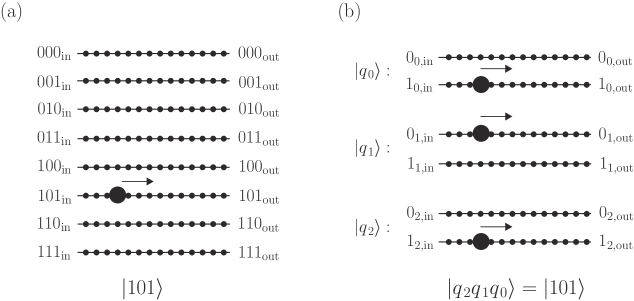
Figure 1: Information spatially encoded by the presence of a quantum walker. (a): A representation used in a single-particle architecture [22]. $2^{n}$ paths are required to express $n$-qubit information. (b): A dual-rail encoding used in [23] and the present work. In contrast to (a), only $2n$ paths are necessary to represent $n$-qubit information. Instead, $n$ walkers are required. Both (a) and (b) express the state $|5\rangle=|101\rangle$. See (2.1) and (2.2) for more precise definition about the dual-rail encoding.

On the other hand, quantum walks can also be viewed as an architecture of quantum computing. Childs [22] has proposed a novel model of universal quantum computation using a continuous-time quantum walk. A quantum walker evolves continuously in time $t$ but discretely in space, according to a unitary operator $e^{-i\mathcal{A}(G)t}$ associated with the adjacency matrix $\mathcal{A}(G)$ for an unweighted graph $G$. An $n$ qubit state is represented by a superposition state in $2^{n}$-dimensional Hilbert space, where the basis state is expressed as the presence of a single quantum walker on any of the $2^{n}$ semi-infinite paths in $G$ (see Fig. 1 (a)). The universal gates are implemented by single-particle scattering processes on a subgraphs $\hat{G}$ connected to $2^{n}$ semi-infinite paths. That is, the outcome of the computation corresponds to the final state of the following process: (i) a quantum walker starts at one of the semi-infinite paths (in superposition) and moves toward $\hat{G}$, (ii) it scatters on $\hat{G}$, and (iii) it goes out to some of semi-infinite paths. Shortly after that, Lovett et al. extended this idea to a discrete-time version of the quantum walk [24, 25].

While the universal gates can be constructed via quantum walks, they cannot be straightforwardly utilized as a practical architecture for a quantum computer because of their lack of scalability: $2^{n}$ paths are required to express $n$ qubits. See Fig. 1 (a), for example. To overcome the difficulty, introducing multi-particle continuous-time quantum walks, Childs, Gosset and Webb have designed a practical model of a quantum computer [23]. They used a so-called dual-rail encoding where a qubit is denoted by the presence of a single quantum walker in either of the two semi-infinite paths (see Fig. 1 (b)). Single-qubit gates are implemented in the same way as the single-particle universal computation. On the other hand, two-qubit gates are realized by a particular combination of single-qubit gates and two-particle scattering of a walker representing the logical qubit from that for the ancilla qubit (see Fig. 6 (b) for an implementation of the controlled-phase (CP) gate). Consequently, the graphs required for the architecture are exponentially smaller than those for single-particle quantum walks. This remarkable progress has been applied to various aspects of quantum computation via quantum walks [26, 27, 28, 29, 30, 31, 32, 33].

In another direction of application of quantum walks to quantum computation, the authors of the present paper have recently proposed a new algorithm for quantum random access memory (qRAM) [34]. A qRAM is a quantum device to access $2^{n}$ $m$-qubit data $|x^{(a)}\rangle_{D}\in(\mathbb{C}^{2})^{\otimes m}$ ($0\leq a\leq 2^{n}-1$) stored in memory cells at addresses $|a\rangle_{A}\in(\mathbb{C}^{2})^{\otimes n}$, and retrieve the data in superposition:

$$\text{qRAM}:\,\,\sum_{a}|a\rangle_{A}|0\rangle_{D}\mapsto\sum_{a}|a\rangle_{A}|x^{(a)}\rangle_{D}.$$ (1.1)

In our algorithm, qRAM is defined on a perfect binary tree with depth $n$, where data and addresses are dual-rail encoded by quantum walkers. The walkers moving in qRAM have two internal states, and depending on their states, a device equipped at each node on the tree (hereafter referred to as a roundabout gate) can properly send the walkers to the designated memory cells placed on the leaves of the tree. As a result, our algorithm requires only $O(n)$ steps and $O(n+m)$ qubit resources to access and retrieve the $2^{n}$ $m$-qubit data. Characteristically, our algorithm promises to require no time-dependent control: qRAM processing is accomplished automatically by simply passing walkers through the binary tree. However, the physical implementation of qRAM, especially how to realize the roundabout gate, has remained a crucial open problem.

The main objectives of the series of two papers are a physical implementation of qRAM using continuous-time multiple quantum walkers with two internal states and a design of a universal quantum computer compatible with this qRAM. The first paper (this one) provides a physical implementation of roundabout gates and uses them to provide a universal set of quantum gates. An efficient physical implementation of qRAM will be presented in the second paper [35].

In our scheme, a single-qubit is spatially represented by a dual-rail encoding as in the above model [23]. On the other hand, the quantum walker can have two internal states $|0\rangle_{\mathrm{c}}$ and $|1\rangle_{\mathrm{c}}$ (e.g., the spin-up and down states of an electron), allowing the physical implementation of a roundabout gate and simplifying the architecture. On the graph $G$, the quantum walkers evolve according to $e^{-i\mathcal{H}_{G}t}$, where $\mathcal{H}_{G}$ is the Hamiltonian associated with the adjacency matrix $\mathcal{A}(G)$ and its complex conjugate $\mathcal{A}(G)^{\ast}$. In contrast to the model in [23], single-particle scattering on a subgraph $\hat{G}$ is used only to implement the roundabout gate that moves a walker clockwise or counterclockwise from one path to the next, depending on the internal state of the walker. A feature of this model is that the roundabout gate also allows the spatial information of the quantum walker to be temporarily encoded in its internal states. Some single-qubit gates are implemented by devices equipped along linear paths, acting on the internal states of walkers. The internal states $|0\rangle_{\mathrm{c}}$ and $|1\rangle_{\mathrm{c}}$ of a walker may coexist only at the moment when the walker passes through a single-qubit gate, and its coherence is completely independent of the other gates.

To implement the roundabout gate, we must consider a scattering on a directed weighted graph $\hat{G}$, which is equivalent to imposing an internal-state-dependent phase factor on the Hamiltonian $\mathcal{H}_{G}$. That is, in the subgraph $\hat{G}$, a walker with $|0\rangle_{\mathrm{c}}$ is evolved by $e^{-i\mathcal{A}(\hat{G})t}$, while a walker with $|1\rangle_{\mathrm{c}}$ is evolved by $e^{-i\mathcal{A}(\hat{G})^{\ast}t}$. This difference allows for the implementation of the roundabout gate. A two-qubit gate is simply realized by an appropriate combination of roundabout gates, single-qubit gates, and two-particle scatterings of fermionic or bosonic walkers with the same internal state. (For instance, see Fig. 6 (a) for the CP gate.) Notably, the calculation is achieved by simply passing quantum walkers through adequately designed paths: there is no need for any time-dependent control. Furthermore, any ancilla qubit required in the model of [23] to implement the two-qubit gates is unnecessary for our architecture. Consequently, we can simplify the architecture compared to the model in [23].

The remainder of the paper is organized as follows. In the subsequent section, we define continuous-time multiple quantum walkers with two internal states. The roundabout gate, playing a pivotal role in our work, is considered in Sec. 3. In Sec. 4, the universal gates are physically implemented by appropriate combinations of roundabout gates, single-qubit gates, and two-particle scatterings. Sec. 5 describes how to construct a practical circuit using a set of quantum gates developed in Sec. 4. Sec. 6 is devoted to a summary. Some applications using the roundabout gate are also discussed. Technical details about scattering theory required in our paper are left in Appendix.

2 Two-level quantum walkers on directed graphs

2.1 General overview

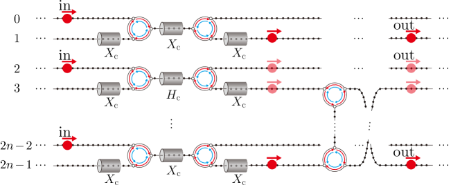
Figure 2: An overview of our architecture for quantum computation. Initial information is represented by the positions of the quantum walkers with internal state $|0\rangle_{\mathrm{c}}$ (see eqs. (2.1) and (2.2)), which are indicated by the red walkers on the left side of the figure. The walkers (wave packets) have momenta $k\simeq-\pi/2$, and move to the right along the semi-infinite paths with group velocity $v_{\mathrm{g}}=E^{\prime}(-\pi/2)=2$, where $E(k)=2\cos k$ (eq. (A.4)) is the energy of each walker. The quantum gates, set up like tunnels, act on the internal states of the walkers passing through them. Some two red walkers are scattered from each other on a vertical path connecting two paths via roundabout gates represented by (2.3) and (2.4). After the scattering, only the global phase of the two-particle wave function is changed. The position state of the quantum walkers after passing through the graph corresponds to the outcome of the computation. Note that the colors of the walkers are temporarily mixed only within single-qubit gates and are set to red otherwise. The colors do not change within the roundabout gates and during the two-particle scatterings.

First, let us present a general overview of our quantum computing architecture via continuous-time quantum walks with two internal states. As shown in Fig. 2, a quantum circuit is spatially designed on a graph on which multiple quantum walkers evolve continuously in time $t$. The dual-rail encoding is employed to represent a single-qubit state as the presence of the quantum walker in one of the two parallel paths. More specifically, a single-qubit state $|q_{j}\rangle$ ($q_{j}\in\{0,1\}$) is given by

$$|q_{j}\rangle=\delta_{q_{j},0}|2j\rangle_{\mathrm{p}}+\delta_{q_{j},1}|2j+1\rangle_{\mathrm{p}}\in\mathbb{C}^{2},$$ (2.1)

where $|j\rangle_{\mathrm{p}}$ ($j\in\{0,\cdots,N-1\}$) denotes the state in which a quantum walker is located on the $j$th path. Thus an $n$-qubit state $|q_{n-1}\cdots q_{0}\rangle$ can be expressed by which of the $2n$ paths the $n$ walkers are located on. Namely,

$$|q_{n-1}\cdots q_{0}\rangle=\bigotimes_{j=0}^{n-1}\Bigl{(}\delta_{q_{j},0}|2j\rangle_{\mathrm{p}}+\delta_{q_{j},1}|2j+1\rangle_{\mathrm{p}}\Bigr{)}\in{(\mathbb{C}^{2})}^{\otimes n}.$$ (2.2)

Note that here and in what follows, we sometimes ignore normalization factors for simplicity of the notation. In our architecture, the quantum walkers have two internal states $|0\rangle_{\mathrm{c}}\in\mathbb{C}^{2}$ and $|1\rangle_{\mathrm{c}}\in\mathbb{C}^{2}$, which are normally set to $|0\rangle_{\mathrm{c}}$ except during processing. For convenience, the quantum walker whose internal state is $|0\rangle_{\mathrm{c}}$ (resp. $|1\rangle_{\mathrm{c}}$) is referred to as the “red quantum walker” (resp. “blue quantum walker”).

Roughly, the computation proceeds as follows. An $n$-qubit input state is prepared by a position state of the red quantum walkers (see the left side in Fig. 2). Then, the walkers move right along the paths, some of which are connected to roundabout gates consisting of a subgraph $\hat{G}_{\mathrm{R}}$. The walker passing through the roundabout gate moves from one path to the next in a clockwise or counterclockwise direction, according to the internal state of the walker. Its unitary operator explicitly reads

$$U_{\mathrm{R}}^{(\mathrm{l})}=|0\rangle\langle 0|_{\mathrm{c}}U_{\mathrm{R}}+|1\rangle\langle 1|_{\mathrm{c}}U^{\dagger}_{\mathrm{R}},\quad U_{\mathrm{R}}^{(\mathrm{r})}=U_{\mathrm{R}}^{(\mathrm{l})}{}^{\dagger},$$

$$U_{\mathrm{R}}=\sum_{k,l=0}^{2}\delta_{l,k+1}|j_{l}\rangle\langle j_{k}|_{\mathrm{p}}\quad(k,l\in\mathbb{Z}/3\mathbb{Z}=\{0,1,2\}),$$ (2.3)

where $U_{\mathrm{R}}^{(\mathrm{l})}$ moves the red walker (resp. blue walker) counterclockwise (clockwise) to the next path, while $U_{\mathrm{R}}^{(\mathrm{r})}$ does the opposite to $U_{\mathrm{R}}^{(\mathrm{l})}$. They can be graphically depicted as

$$\includegraphics[width=242.56108pt]{RA.pdf}.$$ (2.4)

For instance, the red walker (resp. blue walker) entering the $U_{\mathrm{R}}^{(\mathrm{l})}$ (resp. $U_{\mathrm{R}}^{(\mathrm{r})}$ ) gate from path $j_{1}$ (resp. $j_{2}$) exits to path $j_{2}$ (resp. $j_{0}$):

$$\includegraphics[width=220.50885pt]{RAeg.pdf}.$$ (2.5)

The actual implementation of the roundabout gate is achieved by a scattering of a single walker with momentum $k=-\pi/2$ from the graph $\hat{G}_{\mathrm{R}}$ (see Sec. 3 and Appendix). During the scattering, the internal state of the walker never changes, but only by some quantum gates set up like tunnels along the path. For instance, the actions of the Hadamard gate $H_{\mathrm{c}}$ and the Pauli X gate $X_{\mathrm{c}}$ on the state $|0\rangle_{\mathrm{c}}|j\rangle_{\mathrm{p}}$ are respectively written as

$$H_{\mathrm{c}}|0\rangle_{\mathrm{c}}|j\rangle_{\mathrm{p}}=\frac{1}{\sqrt{2}}\bigl{(}|0\rangle_{\mathrm{c}}+|1\rangle_{\mathrm{c}}\bigr{)}|j\rangle_{\mathrm{p}},\quad X_{\mathrm{c}}|0\rangle_{\mathrm{c}}|j\rangle_{\mathrm{p}}=|1\rangle_{\mathrm{c}}|j\rangle_{\mathrm{p}}.$$ (2.6)

They are also graphically shown as

$$\includegraphics[width=308.71104pt]{gate.pdf}.$$ (2.7)

The roundabout gate also serves as an information encoder and decoder: spatial information of the quantum walker can be encoded in the internal state of the walker. For instance,

$$\includegraphics[width=194.04886pt]{encoder.pdf},\includegraphics[width=216.10109pt]{decoder.pdf}.$$ (2.8)

Namely, using the encoder and decoder, we can replace any unitary transformation of single-qubit information with a transformation of the internal state of the quantum walker. Thus, in our architecture, the only non-trivial graph required for quantum walks is the graph used in the roundabout gate, simplifying the structure of the quantum circuit.

See Sec. 4 for more details about the implementation. Some two walkers with the same internal state may be scattered from each other on a straight path (a vertical path in Fig. 2) connecting two paths through roundabout gates. Since the total energy and momentum are conserved, the individual momenta of the two walkers are conserved even after the scattering. As a result, only the global phase of the two-particle wave function can be changed after the scattering. See Sec. 4 and Appendix for the calculation of two-particle scattering processes. The final state obtained after these processes (see the right side in Fig. 2) corresponds to the outcome of the computation. Note again that, in our architecture, the colors of the walkers are in superposition only within each single-qubit gate and are set to red otherwise. In other words, maintaining the coherence of the colors is only necessary within individual single-qubit gates. In actual quantum circuits, the quantum gates must be arranged so that two-particle scatterings occur at the appropriate positions, which will be discussed in Sec. 5.

2.2 Quantum walkers on directed graphs

Now, let us explain the details about the evolution of the quantum walkers on directed weighted graphs. As indicated earlier, spatial dynamics of the quantum walkers required for the computation can be essentially decomposed into motions on semi-infinite paths, single-particle scatterings on subgraph $\hat{G}_{\mathrm{R}}$, and scatterings of two-walkers with same internal state. Hence, the procedure developed in [23, 36] is directly applicable to describe the spatial dynamics of our model. Here and in Appendix, we summarize the procedure to make our paper self-contained and fix the notation.

To formulate the dynamics systematically, we consider the time evolution of the multiple quantum walkers on a generic graph $G=(V,E,w)$ as in [23, 36]. Here $V(G)$ denotes the set of the vertices of $G$, $E(G)\subset V\times V$ is the set of the edges. $w:E\to\mathbb{C}$ is a function defined by $w(x,y)=w_{xy}$ ($x,y\in V(G)$, $(x,y)\in E(G)$), and here is assumed to be

$$w_{xy}=e^{i\theta_{xy}}\,\,(\theta_{xy}\in\mathbb{R}),\quad w_{yx}=w_{xy}^{\ast}=e^{-i\theta_{xy}},\quad w_{xx}=0.$$ (2.9)

The weighted adjacency matrix $\mathcal{A}(G)=(a_{xy})$ is defined by $a_{xy}:=w_{xy}$. In this work, however, we only use the weights $w_{xy}=1$ ($\theta_{xy}=0$) in the semi-infinite paths and $w_{xy}=1$ or $w_{xy}=\pm i$ ($\theta_{xy}=\pm\pi/2$) in a subgraph $\hat{G}$, where $(x,y)\in E(G)$. As shown in Fig. 3 (a), $G$ consists of a subgraph $\hat{G}$ composed by internal vertices, and $N$ semi-infinite paths attached to $\hat{G}$ at the terminal vertices of $\hat{G}$ (depicted them by white circles in Fig. 3 (a)). Let $(x,j)$ ($x\in\mathbb{Z}_{\geq 0}$, $j\in\{0,\cdots,N-1\}$) be the label of the vertex on the $j$th semi-infinite path, located at distance $x$ from $\hat{G}$. $T:=\{(0,j)|0\leq j\leq N-1\}$ denotes the set of the terminal vertices of $\hat{G}$.

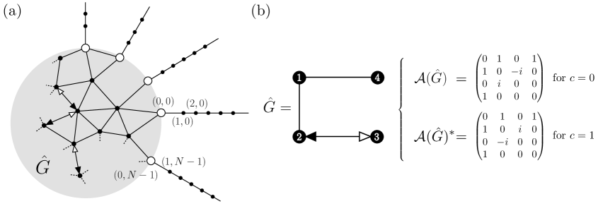
Figure 3: (a): A schematic graph $G$ consisting of a subgraph $\hat{G}$ and $N$ semi-infinite paths connected to $\hat{G}$ (depicted on the gray disk) at the terminals denoted by the white circles. The vertices on the $j$th semi-infinite path are labeled by $(x,j)$ ($x\in\mathbb{Z}_{\geq 0}$, $j\in\{0,\cdots,N-1\}$). (b): An example of the directed subgraph $\hat{G}$ and its adjacency matrix $\mathcal{A}(\hat{G})$. As shown in (2.14), in the subgraph $\hat{G}$, a single red walker ($c=0$) evolves in time according to $e^{-i\mathcal{A}(\hat{G})t}$, while a blue walker ($c=1$) evolves according to $e^{-i\mathcal{A}(\hat{G})^{\ast}t}$.

Let us formulate the dynamics of quantum walkers on the graph $G$, which is governed by the Hamiltonian

$$\mathcal{H}_{G}=\mathcal{K}_{G}+\mathcal{U}_{G}.$$ (2.10)

Here $\mathcal{K}_{G}$ is a kinetic term describing non-interacting walkers, which is defined by

$$\mathcal{K}_{G}=\sum_{c=0,1}\sum_{(x,y)\in E(G)}\left(e^{i(-1)^{c}\theta_{xy}}a_{x,c}^{\dagger}a_{y,c}+e^{-i(-1)^{c}\theta_{xy}}a_{y,c}^{\dagger}a_{x,c}\right),$$ (2.11)

and $\mathcal{U}_{G}$ denotes multiple-particle interactions as explained below (see (2.15)). In the summation, we do not distinguish between $(x,y)$ and $(y,x)$: the sum is taken over either $(x,y)$ or $(y,x)$. $a^{\dagger}_{x,c}$ and $a_{x,c}$ are, respectively, the creation and annihilation operators of walkers of color $c\in\{0,1\}$ on the vertex $x\in V(G)$. The operators satisfy

$$[a_{x,c},a^{\dagger}_{y,c^{\prime}}]_{\mp}=\delta_{x,y}\delta_{c,c^{\prime}},\quad[a_{x,c},a_{y,c^{\prime}}]_{\mp}=[a_{x,c}^{\dagger},a_{y,c^{\prime}}^{\dagger}]_{\mp}=0,$$ (2.12)

where $[\cdot,\cdot]_{-}$ and $[\cdot,\cdot]_{+}$ denote the commutator for the boson operators and anticommutator for the fermion operators, respectively. The creation operators $a_{x,c}^{\dagger}$ generate the Hilbert space $H^{(m)}$ for $m$ quantum walkers on $G$: $H^{(m)}$ is spanned by the basis vectors

$$\left.\left\{|c_{1}\cdots c_{m}\rangle_{\mathrm{c}}|x_{1}\cdots x_{m}\rangle:=a^{\dagger}_{x_{m},c_{m}}\cdots a^{\dagger}_{x_{1},c_{1}}|0\rangle\,\right|c_{1},\cdots,c_{m}\in\{0,1\},\,x_{1},\cdots,x_{m}\in V(G)\right\},$$ (2.13)

where $|0\rangle$ is the no-walker state (vacuum state) defined by $a_{x,c}|0\rangle=0$ $(c\in\{0,1\}\,\,\,x\in V(G))$. The notation $|x,j\rangle$ is also used to denote the walker at $(x,j)$, i.e., at $x\in\mathbb{Z}_{\geq 0}$ on path $j$ ($j\in\{0,\cdots,N-1\}$). The time-evolution of the $m$ quantum walkers on the graph $G$ is described by the action of the unitary operator $e^{-i\mathcal{H}_{G}t}$ on a vector in the Hilbert space $H^{(m)}$. Information of the adjacency matrix $\mathcal{A}(G)=(e^{i\theta_{xy}})$ ($\theta_{xy}\in\{0,\pm\pi/2\}$, $(x,y)\in E(G)$) of the graph $G$ is incorporated into the kinetic term $\mathcal{K}_{G}$ (2.11) as

$$(\mathcal{K}_{G})_{cc^{\prime},\,xy} :={}_{\mathrm{c}}\langle c|\langle x|\mathcal{K}_{G}|c^{\prime}\rangle_{\mathrm{c}}|y\rangle$$

$$=(e^{i\theta_{xy}}\delta_{c,0}\delta_{c^{\prime},0}+e^{-i\theta_{xy}}\delta_{c,1}\delta_{c^{\prime},1})\delta_{(x,y)\in E(G)}$$

$$=(\mathcal{A}(G))_{xy}\delta_{c,0}\delta_{c^{\prime},0}+(\mathcal{A}(G)^{\ast})_{xy}\delta_{c,1}\delta_{c^{\prime},1}.$$ (2.14)

Importantly, in the directed weighted graph $\hat{G}$, the time-evolution of a walker depends explicitly on its internal state: the evolution of a red walker (i.e., $c=0$) is described by the unitary operator $e^{-i\mathcal{A}(\hat{G})t}$, while that of a blue walker (i.e., $c=1$) is described by $e^{-i\mathcal{A}(\hat{G})^{\ast}t}$. See also Fig. 3 (b) for an example of $\hat{G}$. It is this difference that makes the physical implementation of the roundabout gate possible. Physically, the weight $w_{xy}=e^{i\theta_{xy}}$ in (2.11) can be interpreted as a phase factor under a local gauge transformation $a_{x,c}\mapsto e^{i\vartheta_{x,c}}a_{x,c}$ ($\vartheta_{x,c}\in\mathbb{R}$), which may be achieved, for example, by applying the Aharonov-Kasher effect [37, 38].

Two-qubit gates are realized by taking into account two-particle scatterings of fermionic or bosonic walkers with the same internal state. To this end, as in [23], we adopt the on-site interaction (Bose-Hubbard model) for the bosonic case and the nearest-neighbor interaction (extended Hubbard model) for the fermionic case:

$$\mathcal{U}_{G}=\begin{dcases}\frac{u}{2}\sum_{x\in V(G)}n_{x}(n_{x}-1)&\text{ for the bosonic walkers}\\ u\sum_{(x,y)\in E(G)}n_{x}n_{y}&\text{ for the fermionic walkers}\end{dcases},$$ (2.15)

where $n_{x}:=\sum_{c=0}^{1}a_{x,c}^{\dagger}a_{x,c}$ is the number operator.

As an actual implementation, we consider a quantum walker as a wave packet $|\Psi,t\rangle=e^{-i\mathcal{H}_{G}t}|\Psi\rangle$ constructed by a superposition of plane waves with momentum $k$ close to a specific value of $k_{\mathrm{p}}$. For instance, a wave packet on a semi-infinite path (the actual implementation uses a sufficiently long path) toward a subgraph $\hat{G}$ is given by

$$|\Psi,t\rangle =\sum_{x}\frac{1}{\sqrt{2\pi}}\int_{k\simeq k_{\mathrm{p}}}dkf(k)e^{-ikx-iE(k)t}|c\rangle_{\mathrm{c}}|x\rangle$$

$$\simeq\sum_{x}\frac{e^{-ik_{\mathrm{p}}x-iE(k_{\mathrm{p}})t}}{\sqrt{2\pi}}\int_{k\simeq k_{\mathrm{p}}}dkf(k)e^{-i(k-k_{\mathrm{p}})(x+E^{\prime}(k_{\mathrm{p}})t)}|c\rangle_{\mathrm{c}}|x\rangle,$$ (2.16)

where $f(k)$ is the Fourier coefficient with a sharp peak at $k\simeq k_{\mathrm{p}}$, and $E(k)=2\cos k$ (eq. (A.4)) is the energy of the quantum walker on the semi-infinite path. The wave packet moves with the group velocity $E^{\prime}(k_{\mathrm{p}})=-2\sin k_{\mathrm{p}}$. To make our purpose, in the current work, we assign $k\simeq k_{\mathrm{p}}=-\pi/2$ to the momentum of each walker.

Quantum computation is performed by applying unitary transformations to wave packets (2.16). What is crucial then is how to add the overall phase factor to each wave packet (note that simply translating the wave packet (2.16) as $x\mapsto x+a$ does not yield this), and how to superpose them. In our architecture, for a single quantum walker, this manipulation is essentially accomplished by unitary transformations to the internal state of the walker, and when two walkers are involved, as in controlled gates, this is accomplished by two-particle scattering. Single-particle scattering is used only for the implementation of the roundabout gate whose primary role is to switch the position of the walker. See Sec. 4 for details. This is in contrast to the architecture [23], where all unitary transformations are performed by single-particle and two-particle scatterings. In Appendix, we summarize single- and two-particle scatterings with a definite momentum $k$ (i.e., scatterings of plane waves) which are key to understanding the scattering processes of wave packets with momentum close to $k$.

3 Roundabout gate

The roundabout gate (2.3) or (2.4) is the most crucial element in our architecture. As schematically depicted in (2.5), the walker passing through the roundabout gate can move from one path to the next. In this section, we implement the roundabout gate $U_{\mathrm{R}}^{(\mathrm{l})}$ with single-particle scattering: we find a graph $\hat{G}_{\mathrm{R}}$ such that the $S$-matrix $S(k)$ (resp. $\tilde{S}(k)$) describing the scattering of the red walker (resp. blue walker) on $\hat{G}_{\mathrm{R}}$ satisfies $S(k)=U_{\mathrm{R}}$ (resp. $\tilde{S}(k)=U^{\dagger}_{\mathrm{R}}$) for some specific value of $k$, where $U_{\mathrm{R}}$ is defined by (2.3). In fact, the scattering process only for the red walker is sufficient to study, because the $S$-matrix $\tilde{S}(k)$ for the blue walker is nothing but the transpose of the $S$-matrix $S(k)$ for the red walker, as shown in Appendix (see (A.9)). Additionally, the color of the walkers does not change during the single-particle scattering, which can be seen by the Hamiltonian (2.10), especially the kinetic term (2.11). A physical implementation of another type of roundabout gate $U_{\mathrm{R}}^{(\mathrm{r})}(:=U_{\mathrm{R}}^{(\mathrm{l})}{}^{\dagger})$ in (2.3) can be easily accomplished by replacing the subgraph $\hat{G}_{\mathrm{R}}$ with $\hat{G}^{\ast}_{\mathrm{R}}$ whose adjacency matrix is given by $\mathcal{A}(\hat{G}^{\ast}_{\mathrm{R}})=\mathcal{A}(\hat{G}_{\mathrm{R}})^{\ast}$.

The $S$-matrix $S(k)$ of the red walker characterizing the scattering state is expressed in terms of the elements of the adjacency matrix $\mathcal{A}(\hat{G}_{\mathrm{R}})$, as shown in (A.7), which serves as a clue to find the desired adjacency matrix. (See Appendix for scattering theory required in this section.) Using (A.7), we find that the following three graphs

(3.1)

with the abbreviation of the directed weighted edge

(3.2)

all implement the roundabout gate up to the sign (the minus sign is necessary for $\hat{G}_{\mathrm{R}}^{(1)})$, when the momentum of the walker passing through them is exactly $k=-\pi/2$: $S(-\pi/2)=U_{\mathrm{R}}$ for the red walker and $\tilde{S}(-\pi/2)=S(-\pi/2)^{\mathrm{T}}=U^{\dagger}_{\mathrm{R}}$ (cf. (A.9)) for the blue walker. More explicitly, the matrix elements of $S(k)=\sum_{m,n}S_{mn}(k)|0,m\rangle\langle 0,n|$ are given by

$$S_{00}(k)=\frac{-e^{4ik}}{1+2i\tan k},\,\,\, S_{10}(k)=\frac{-2e^{\frac{7ik}{2}-\frac{i\pi}{4}}\cos\left(\frac{k}{2}+\frac{\pi}{4}\right)}{2-i\cot k},\,\,\, S_{20}(k)=\frac{-2ie^{\frac{7ik}{2}-\frac{i\pi}{4}}\sin\left(\frac{k}{2}+\frac{\pi}{4}\right)}{2-i\cot k},$$

$$S_{11}(k)=S_{00}(k),\,\,\, S_{21}(k)=S_{10}(k),\,\,\, S_{22}(k)=S_{00}(k),$$ (3.3)

for $\hat{G}^{(1)}_{\mathrm{R}}$ and

$$S_{00}(k)=\frac{-e^{4ik}}{1+2i\tan k},\,\,\, S_{10}(k)=\frac{2e^{\frac{7ik}{2}-\frac{i\pi}{4}}\cos\left(\frac{k}{2}+\frac{\pi}{4}\right)}{2-i\cot k},\,\,\, S_{20}(k)=\frac{2e^{\frac{9ik}{2}-\frac{i\pi}{4}}\sin\left(\frac{k}{2}+\frac{\pi}{4}\right)}{2-i\cot k},$$

$$S_{11}(k)=S_{00}(k),\,\,\, S_{21}(k)=\frac{2e^{\frac{9ik}{2}+\frac{i\pi}{4}}\cos\left(\frac{k}{2}+\frac{\pi}{4}\right)}{2-i\cot(k)},\,\,\, S_{22}(k)=e^{2ik}S_{00}(k),$$ (3.4)

for $\hat{G}^{(2)}_{\mathrm{R}}$ and $\hat{G}^{(3)}_{\mathrm{R}}$. The other elements are determined by the relation $S(k)=S(-k)^{\dagger}$ which holds for $k\in\mathbb{R}$ (see (A.8)).

The probability that a walker entering $\hat{G}_{\mathrm{R}}$ from path $m\in\mathbb{Z}/3\mathbb{Z}=\{0,1,2\}$ will be found on path $n\in\mathbb{Z}/3\mathbb{Z}=\{0,1,2\}$ is given by $|S_{mn}(k)|^{2}$, which is the same for all three cases in (3.1). We see that the walker with momentum $k=-\pi/2$ perfectly transmits from $n$ to $m=n+1$. In Fig. 4, the momentum dependence of the transmission probabilities are shown. In summary, the subgraphs $G^{(j)}_{\mathrm{R}}$ and $G^{\ast(j)}_{\mathrm{R}}$ ($j=1,2,3$) are, respectively, physical implementations of the roundabout gates $U_{\mathrm{R}}^{(\mathrm{l})}$ and $U_{\mathrm{R}}^{(\mathrm{r})}$ for a quantum walker with momentum $k=-\pi/2$. Graphically,

$$\includegraphics[width=176.40439pt]{URl_G.pdf},\quad\includegraphics[width=176.40439pt]{URr_Gstar.pdf}$$ (3.5)

The same is true for $G^{(j)}_{\mathrm{R}}$ and $G^{\ast(j)}_{\mathrm{R}}$ ($j=2,3$) as above. Note that $\hat{G}^{\ast}_{\mathrm{R}}$ is obtained by reversing all the arrows in $\hat{G}_{\mathrm{R}}$ (eq. (3.1)), because $\mathcal{A}(\hat{G}^{\ast}_{\mathrm{R}})=\mathcal{A}(\hat{G}_{\mathrm{R}})^{\ast}$.

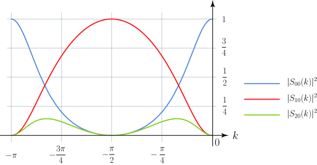
Figure 4: The momentum dependence of the probability $|S_{m0}(k)|^{2}$ ($m=0,1,2$) that a walker entering $\hat{G}_{\mathrm{R}}^{(j)}$ ($j\in\{1,2,3\}$) (3.1) from path $0$ will be found on path $m$ ($m=0,1,2$). The walker with momentum $k=-\pi/2$ completely transmits from path $0$ to path $1$.

In the actual implementation, we use a wave packet (2.16) as a quantum walker and consider the scattering state on the subgraph $\hat{G}_{\mathrm{R}}$ with sufficiently long (but finite length) paths attached. The effective length of the subgraph $\hat{G}_{\mathrm{R}}$ can be evaluated by the non-trivial phase shift of the wave packet output from $\hat{G}_{\mathrm{R}}$ after scattering. The wave packet $|\Psi_{\mathrm{out}},t\rangle$ for the red walker exiting from $(0,l)$, which entered $\hat{G}_{\mathrm{R}}$ from $(0,j)$ (cf. (A.1) and (2.16)), is given by

$$|\Psi_{\mathrm{out}},t\rangle =\frac{1}{\sqrt{2\pi}}\int_{k\simeq k_{\mathrm{p}}}dkS_{lj}(k)f(k)e^{ikx-iE(k)t}|0\rangle_{\mathrm{c}}|x\rangle$$

$$\simeq\frac{S_{lj}(k_{\mathrm{p}})e^{ik_{\mathrm{p}}x-iE(k_{\mathrm{p}})t}}{\sqrt{2\pi}}\int_{k\simeq k_{\mathrm{p}}}dkf(k)e^{i(k-k_{\mathrm{p}})(x-i(\log S_{lj})^{\prime}(k_{\mathrm{p}})-E^{\prime}(k_{\mathrm{p}})t)}|0\rangle_{\mathrm{c}}|x\rangle.$$ (3.6)

Thus, the effective length

$$\ell_{lj}(k):=-i(\log S_{lj})^{\prime}(k)$$ (3.7)

for the red walker is calculated by (3.3) or (3.4):

$$\ell_{lj}\left(-\frac{\pi}{2}\right)=3\delta_{l,j+1}\text{ for $G_{\mathrm{R}}^{(1)}$},\quad\ell_{lj}\left(-\frac{\pi}{2}\right)=\begin{cases}3\delta_{l,j+1}&\text{for $j=0$}\\ 4\delta_{l,j+1}&\text{for $j=1,2$}\end{cases}\text{ for $G_{\mathrm{R}}^{(2)}$ and $G_{\mathrm{R}}^{(3)}$},$$ (3.8)

where $j,l\in\mathbb{Z}/3\mathbb{Z}=\{0,1,2\}$. On the other hand, the effective length $\tilde{\ell}_{lj}(k)$ for the blue walker is given by the relation

$$\tilde{\ell}_{lj}(k)=\ell_{jl}(k)\quad(k\in\mathbb{R}),$$ (3.9)

which follows from (A.9). These effective lengths are necessary for building actual finite-size quantum circuits, where a synchronization of the motion of quantum walkers becomes crucial. See Sec. 5 for details.

4 Elementary quantum gates

In this section, we describe how to implement a universal quantum gate set via two-level quantum walkers. As described in Sec. 2, information is spatially encoded by the positions of red quantum walkers. Information processing is carried out by moving multiple quantum walkers to appropriate positions. In our architecture, the internal state of the quantum walker serves as a temporal storage medium during this process. Any unitary transformation to a single-qubit state can be replaced by a transformation to the internal state of the quantum walker. There, the roundabout gate not only switches the position of the walkers but acts as an information encoder and decoder. In addition, combining two-particle scattering on an infinite path, one can implement a controlled gate.

4.1 Single-qubit gates

First, let us implement a unitary operator $U$ acting on a single-qubit state $|q_{j}\rangle$ defined as (2.1). In our scheme, we express the state as the position of the red quantum walker:

$$|0\rangle_{\mathrm{c}}|q_{j}\rangle=|0\rangle_{\mathrm{c}}|2j+q_{j}\rangle_{\mathrm{p}}\in\mathbb{C}^{2}\otimes\mathbb{C}^{2}.$$ (4.1)

The information $|q_{j}\rangle$ can be encoded into the internal state of the walker passing through the following encoder $U_{\mathrm{E}}$ which consists of the Pauli X gate $X_{\mathrm{c}}$ (eq. (2.7)) and the roundabout gate $U_{\mathrm{R}}^{(\mathrm{r})}$ (eq. (2.4)):

$$\begin{array}[]{c}\includegraphics[width=308.71104pt]{UE.pdf}\end{array}.$$ (4.2)

Let us explain in detail. A red walker prepared on the $(2j)$th or $(2j+1)$th input path (possibly in superposition) moves toward the roundabout gate $U_{\mathrm{R}}^{(\mathrm{r})}$; the red walker on the $(2j+1)$th path changes color to blue at the $X_{\mathrm{c}}$ gate before entering $U_{\mathrm{R}}^{(\mathrm{r})}$. The roundabout gate $U_{\mathrm{R}}^{(\mathrm{r})}$ consists of the subgraph $\hat{G}_{\mathrm{R}}^{\ast}$ moves the red walker (resp. blue walker) clockwise (resp. counterclockwise) to output path $j^{\prime}$, as shown in the previous section. For example, the inset depicts $\hat{G}^{\ast(1)}_{\mathrm{R}}$ (cf. (3.5)). The effective length of $U_{\mathrm{R}}^{(\mathrm{r})}$ can be exactly the same for the red and blue walkers, if the terminal vertices $(0,j)$ $(j\in\{0,1,2\})$ of $\hat{G}_{\mathrm{R}}^{\ast}$ as in (3.5) and (3.1) are connected to paths $\{2j,2j+1,j^{\prime}\}$ in (4.2) so that $(0,0)\to(0,2j)$, $(0,1)\to(0,2j+1)$ and $(0,2)\to(0,j^{\prime})$. More precisely, one finds

$$\ell_{j^{\prime},2j}\left(-\frac{\pi}{2}\right)=\tilde{\ell}_{j^{\prime},2j+1}\left(-\frac{\pi}{2}\right)=\begin{cases}3&\text{for $\hat{G}^{\ast(1)}_{\mathrm{R}}$}\\ 4&\text{for $\hat{G}^{\ast(2)}_{\mathrm{R}}$ and $G^{\ast(3)}_{\mathrm{R}}$ }\\ \end{cases},$$ (4.3)

where $\ell_{j^{\prime},2j}(-\pi/2)$ and $\tilde{\ell}_{j^{\prime},2j+1}(-\pi/2)$ are, respectively, the effective lengths of $U_{\mathrm{R}}^{(\mathrm{r})}$ for the red and blue walker. This is derived from (3.8), (3.9) and the fact that the $S$-matrix for $\hat{G}^{\ast}_{\mathrm{R}}$ is given by the transpose of that for $\hat{G}_{\mathrm{R}}$, as shown in (A.9). Eq. (4.2) equivalently reads

$$\eqref{dual-internal}\xmapsto{X_{\mathrm{c}}\otimes(|2j+1\rangle\langle 2j+1|_{\mathrm{p}})}\delta_{q_{j},0}|0\rangle_{\mathrm{c}}|2j\rangle_{\mathrm{p}}+\delta_{q_{j},1}|1\rangle_{\mathrm{c}}|2j+1\rangle_{\mathrm{p}}\xmapsto{U_{\mathrm{R}}^{(\mathrm{r})}}|q_{j}\rangle_{\mathrm{c}}|j^{\prime}\rangle_{\mathrm{p}}.$$ (4.4)

Applying a unitary gate $U_{\mathrm{c}}$ to the internal state of the walker moving in the right direction on path $j^{\prime}$, and then applying the decoder $U_{\mathrm{D}}$ (eq. (2.8)) realized by the reverse operation of the encoder $U_{\mathrm{E}}$ (eq. (4.2)) (i.e., $U_{\mathrm{D}}=U_{\mathrm{E}}^{\dagger}$), we obtain the desired state $U|q_{j}\rangle$:

$$\eqref{encoder2}\xmapsto{U_{\mathrm{c}}}\left(U_{\mathrm{c}}|q_{j}\rangle_{\mathrm{c}}\right)|j^{\prime}\rangle_{\mathrm{p}}\xmapsto{U_{\mathrm{D}}=U_{\mathrm{E}}^{\dagger}}|0\rangle_{\mathrm{c}}(U|q_{j}\rangle).$$ (4.5)

Graphically, the single-qubit gate is depicted as

$$\begin{array}[]{c}\includegraphics[width=343.99327pt]{U.pdf}.\end{array}$$ (4.6)

It is known [39, 40] that any single-qubit unitary gate $U$ is realized by

$$U=e^{i\theta_{0}}R_{z}(\theta_{1})R_{y}(\theta_{2})R_{z}(\theta_{3})\quad(\theta_{j}\in\mathbb{R}),$$ (4.7)

where

$$R_{y}(\theta):=\exp\left(-i\frac{\theta Y}{2}\right),\quad R_{z}(\theta):=\exp\left(-i\frac{\theta Z}{2}\right)$$ (4.8)

are, respectively, the rotation operators about $y$ and $z$ axes of the Bloch sphere; $Y$ and $Z$ are the Pauli matrices $\sigma_{y}$ and $\sigma_{z}$, respectively.

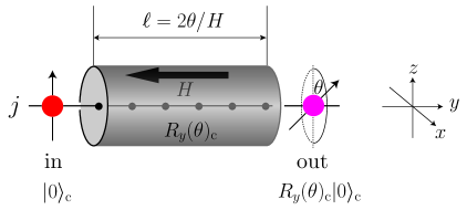
Figure 5: A schematic description of the rotation gate $R_{y}(\theta)_{\mathrm{c}}$ for the spin-1/2 fermionic system. A uniform magnetic field $H$ is applied in the negative direction of the $y$-axis in the device set up like tunnels along the path. Since the speed of the walker is $v_{\mathrm{g}}=2$ (eq. (4.9)) and the Zeeman energy $\mathcal{H}_{\mathrm{ex}}=H\sigma_{y}/2=HY/2$, $R_{y}(\theta)_{\mathrm{c}}=e^{-i\theta Y_{\mathrm{c}}/2}$ is implemented by just setting the length of the device to $\ell=2\theta/H$.

Actually, for instance, in the spin-1/2 fermionic system, the rotation gates acting on the spin state may be implemented by applying a uniform magnetic field $H$ in a particular direction over a suitable interval of the path. See Fig. 5 for a schematic description of a rotation gate $R_{y}(\theta)_{\mathrm{c}}$ acting on the internal state of the walker. Since the Zeeman energy $\mathcal{H}_{\mathrm{ex}}$ is given by $\mathcal{H}_{\mathrm{ex}}=HY/2$ (resp. $\mathcal{H}_{\mathrm{ex}}=HZ/2$) for the magnetic field $H$ applied in the negative direction of the $y$-axis (resp. $z$-axis), the spin state of the walker passing through the device over time $t$ is transformed by the operator $R_{y}(Ht)_{\mathrm{c}}=e^{-itHY_{\mathrm{c}}/2}$ (resp. $R_{z}(Ht)_{\mathrm{c}}=e^{-itHZ_{\mathrm{c}}/2}$). Because the (group) velocity $v_{\mathrm{g}}$ of the quantum walker with momentum $k=-\pi/2$ is

$$v_{\mathrm{g}}=E^{\prime}\left(-\frac{\pi}{2}\right)=-2\sin\left(-\frac{\pi}{2}\right)=2$$ (4.9)

(see (A.4)), $R_{y,z}(\theta)_{\mathrm{c}}$ can be implemented by just setting the device length $\ell$ so that $\theta=tH=\ell H/v_{\mathrm{g}}$, i.e., $\ell=2\theta/H$.

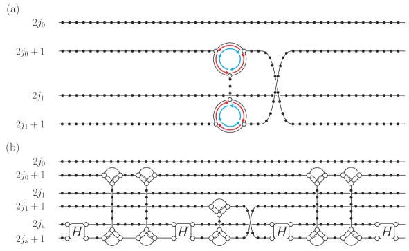
Figure 6: (a): A controlled-phase (CP) gate (4.11) implemented in the present model. (b): The CP gate implemented in the model [23]. In contrast to (b), single-particle scattering is used in (a) only for the implementation of the roundabout gate. Since (a) does not require ancilla qubits (corresponding to $|2j_{\mathrm{a}}\rangle_{\mathrm{p}}$ and $|2j_{\mathrm{a}}+1\rangle_{\mathrm{p}}$ in (b)), the architecture can be drastically simplified compared to (b).

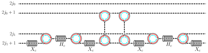
Figure 7: A graphical representation of the CNOT gate (4.10).

4.2 Two-qubit gates

Appropriately combining the scattering of two walkers with the same internal state and a single-qubit gate described above, we can implement a two-qubit gate. The aforementioned single-qubit rotation gates and a controlled-NOT (CNOT) gate are elements of a universal gate set [39, 40]. In fact, the CNOT gate $\mathrm{CNOT}_{j_{0}j_{1}}$ acting on a two-qubit state $|q_{j_{1}}\rangle|q_{j_{0}}\rangle$ is decomposed into

$$\mathrm{CNOT}_{j_{0}j_{1}}=H_{j_{1}}\mathrm{CP}^{2}_{j_{0}j_{1}}H_{j_{1}},$$ (4.10)

where $H_{j_{1}}$ is the Hadamard gate on $|q_{j_{1}}\rangle$ and $\mathrm{CP}_{j_{0}j_{1}}$ is a controlled phase (CP) gate on $|q_{j_{1}}\rangle|q_{j_{0}}\rangle$:

$$\mathrm{CP}=\begin{pmatrix}1&0&0&0\\ 0&1&0&0\\ 0&0&1&0\\ 0&0&0&\pm i\end{pmatrix}.$$ (4.11)

As explained earlier, the action of $H_{j_{1}}$ can be replaced by the action on the internal state of the quantum walker moving along path $j_{1}^{\prime}$, which is connected to paths $2j_{1}$ and $2j_{1}+1$ by roundabout gates. The CP gate, on the other hand, is implemented by two-particle scattering on an infinite path: two particles, respectively moving along paths $2j_{0}+1$ and $2j_{1}+1$, are switched by the roundabout gate to the same infinite path and travel toward each other with momenta $k_{0}=-\pi/2$ and $k_{1}=\pi/2$ to be scattered from each other. Due to the conservation laws of energy and momentum, the individual momenta are also conserved after scattering. As a result, only the global phase of the two-particle wave function can be changed. In Appendix, we evaluate the phase for both the bosonic and fermionic cases. For the bosonic system with $u=\mp 4$ in the interaction term (2.15), the wave function acquire a phase $S_{01}(k_{0}=-\pi/2,k_{1}=\pi/2)=\pm i$ after scattering (see (A.15)). For the fermionic case, a global phase $S_{01}(k_{0}=-\pi/2,k_{1}=\pi/2)=\pm i$ is acquired for $u=\mp 2$. Consequently, the CP gate is implemented by two roundabout gates as depicted in Fig. 6. Characteristically, our architecture does not require any ancilla qubit; therefore the structure of controlled gates can be significantly simplified, compared to those in [23]. Finally, we graphically represent the CNOT gate (4.10) in Fig. 7.

In the actual implementation of the two-qubit gates, we use wave packets (2.16) as quantum walkers and consider the scattering state on a sufficiently long (but finite length) paths. The effective length $\ell(-\pi/2)$ for each walker in the two-particle scattering is obtained via (A.11), (A.15) and (A.18):

$$\ell\left(-\frac{\pi}{2}\right) =-i{\partial}_{k_{0}}\log S\left(k_{0}=-\frac{\pi}{2},k_{1}=\frac{\pi}{2}\right)=i{\partial}_{k_{1}}\log S\left(k_{0}=-\frac{\pi}{2},k_{1}=\frac{\pi}{2}\right)$$

$$=\begin{cases}0&\text{for boson}\\ -1/2&\text{for fermion}\end{cases}.$$ (4.12)

Finally, we would like to comment on the reversibility of our architecture. Since the adjacency matrix of the graph used in the current architecture is a Hermitian matrix, the time evolution of the quantum walkers is of course described by a unitary operator. In this sense, quantum computation using the present model is as reversible as ordinary quantum computers. However, simply reversing the motions of the walkers on the output paths (i.e., giving them the opposite momenta) is not enough to return them to their initial positions on the input paths. To return them to their original positions, one must not only reverse the motions of the walkers, but also replace the clockwise roundabout gates with counterclockwise roundabout gates, and vice versa. Alternatively, we can also return them to the original positions by changing the colors of the walkers on the output paths from red (spin-up) to blue (spin-down), reversing the direction of all the magnetic fields applied in the single-qubit devices (see Fig. 5), and reversing the motions of the walkers (i.e., time reversal symmetry).

5 Building a circuit

The quantum walker is effectively realized by a wave packet consisting of plane waves with momentum close to a specific value of $k\simeq k_{\mathrm{p}}$ (see (2.16), for instance). As explained earlier, in our architecture, $k_{\mathrm{p}}=-\pi/2$ is assigned to design quantum gates. To build a quantum circuit for practical use, we must truncate the semi-infinite paths connected to each subgraph and consider scatterings of wave packets on a finite-size graph (circuit). There, the timing of the two-particle scatterings becomes crucial: the two-particle scatterings must occur at the proper vertical paths. Here, we explain how to arrange the quantum gates to build a practical circuit, according to the procedure developed in [23]. Also an error bound is estimated.

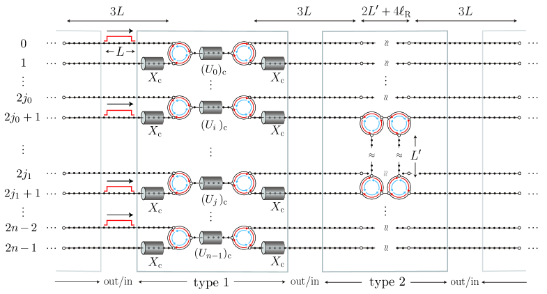
Figure 8: In the actual $n$-qubit circuit, $n$ wave packets of length $L$ are employed as quantum walkers to represent an $n$-qubit state. Any circuit can be built by a proper combination of type 1 and type 2 blocks. A block of type 1 consists of $n$ single qubit gates $U_{0},\cdots,U_{n-1}$ (some of which may be identity gates). A block of type 2 consists of a set of CP gates $\mathrm{CP}_{j_{0}j_{1}}$ ($j_{0}\neq j_{1}$, $j_{0},j_{1}\in\{0,\cdots,n-1\}$) constructed by four roundabout gates. An identity gate in a block of type 2 is realized by simply connecting the input and output of the block with a straight path of length $2L^{\prime}+4\ell_{\mathrm{R}}$, where $L^{\prime}\geq 4L$ is the length of each vertical path connecting the upper and lower two roundabout gates within each CP gate, and $\ell_{\mathrm{R}}$ is the effective length of the roundabout gate (see (3.8)). Input/output paths of length $3L$ each are attached to each block, where the output paths of one block are commonly used as the subsequent block.

Let us build an $n$-qubit circuit. Any quantum circuit can be designed by appropriately combining blocks consisting of single-qubit gates (“type 1 blocks”) and blocks consisting of CP gates (“type 2 blocks”), as depicted in Fig. 8. The input/output $n$-qubit state $|q_{n-1}\cdots q_{0}\rangle$ ($q_{j}\in\{0,1\},\,\,j\in\{0,\cdots,n-1\}$) of each block is dual-rail encoded by $n$ red quantum walkers (cf. (4.1)), given by the following wave packet of length $L$:

$$|q_{j}\rangle=\frac{1}{\sqrt{L}}\sum_{x=L}^{2L-1}e^{\pm i\frac{\pi}{2}x}|0\rangle_{\mathrm{c}}|x,2j+q_{j}\rangle_{\mathrm{in/out}},$$ (5.1)

where $|x,j\rangle_{\mathrm{in/out}}$ denotes the position state of a particle on the $j$th input/output path and the positive and negative signs in the exponential correspond to the input and output wave packets, respectively. Also, the length of each input/output path connecting to each block is set to $3L$, and the output paths of one block are commonly used as the input paths for the subsequent block. The state (5.1) is expressed as the wave packet located in the center of each path. Incidentally, the input wave packet (5.1) itself is given by the superposition of plane waves (2.16) with the probability amplitude:

$$f(k)=\sqrt{\frac{2}{L\pi}}\frac{\sin\left(\frac{L-1}{2}(k+\frac{\pi}{2})\right)}{k+\frac{\pi}{2}}e^{\frac{3L-1}{2}\left(k+\frac{\pi}{2}\right)i}.$$ (5.2)

Now let us consider how the quantum gates in blocks of type 1 and type 2 can be arranged so that the desired pair of red walkers can meet simultaneously on a particular vertical path. As shown in Fig. 8, a block of type 1 consists of $n$ single-qubit gates $U_{0},\cdots,U_{n-1}$ (some of which may be identity gates), in which $(U_{j})_{\mathrm{c}}$ acts on the internal state of the walker transferred from path $2j$ or $2j+1$ by the leftmost roundabout gate. As explained in Sec. 4, it is possible to make the effective lengths of the roundabout gates for the red and blue walkers exactly the same by incorporating the graphs $\hat{G}_{\mathrm{R}}$ and $\hat{G}^{\ast}_{\mathrm{R}}$ in the proper orientation. If the quantum gates are assembled in such a manner, quantum walkers that simultaneously enter a block of type 1 will exit that block at the same time. In other words, type 1 blocks do not affect the order of walkers.

A block of type 2 consists of a set of CP gates $\mathrm{CP}_{j_{0}j_{1}}$ ($j_{0}\neq j_{1}$, $j_{0},j_{1}\in\{0,\cdots,n-1\}$) and identity gates. In contrast to a block of type 1, an identity gate is realized by simply connecting the input and output with a straight path. As a CP gate, we employ

$$\mathrm{CP}_{j_{0}j_{1}}=\begin{pmatrix}1&0&0&0\\ 0&1&0&0\\ 0&0&1&0\\ 0&0&0&-1\end{pmatrix}_{j_{0}j_{1}}$$ (5.3)

instead of (4.11), taking into account the effective length (4.12) of the two-particle scattering of fermionic walkers . This CP gate is achieved by placing four roundabout gates as shown in Fig. 8. The right terminal vertex on path $2j_{0}+1$ or $2j_{1}+1$ of the left roundabout gate can be directly connected to the right terminal vertex of the right roundabout gate without compromising the function of the gate. Let us set the length of each vertical path to $L^{\prime}\geq 4L$ and denote the effective length of each roundabout gate by $\ell_{\mathrm{R}}$ (i.e., $\ell_{\mathrm{R}}=3$ or $\ell_{\mathrm{R}}=4$ from (3.8)). Then, if we set the length of the straight path of the identity gate to $2L^{\prime}+4\ell_{\mathrm{R}}$, a particular pair of red walkers simultaneously entering the block can be scattered within a specific vertical path. In addition, for the fermionic walks, we must take into account the effective length (4.12) of the two-particle scattering: the scattered fermionic walkers in the CP gate move ahead of other walkers by one vertex. In this case, by increasing the number of vertices in each horizontal and vertical path by one in the next type 2 block, the desired two-particle scattering can occur within a specific vertical path in the next block. Namely, in the $m$th type 2 block, the number of vertices in each horizontal and vertical path should be increased by $m$ more than in the first.

As explained in Sec. 3 and 4, the roundabout gate and the CP gate are designed based on single- and two-particle scattering states of plane waves with a definite momentum $k=k_{\mathrm{p}}$, which are defined on the subgraph with semi-infinite path and on the straight vertical path of infinite length, respectively. Therefore, to ensure the reliability of the architecture, it is also essential to estimate errors that occur in an actual quantum circuit consisting of a finite-size graph on which the wave packets move as quantum walkers. Let $|\Psi_{\mathrm{in}}\rangle$ be an input state in superposition (cf. (5.1)):

$$|\Psi_{\mathrm{in}}\rangle=\frac{1}{\sqrt{L}}\sum_{\{q_{j}\}}\bigotimes^{n-1}_{j=0}\left(\sum_{x=L}^{2L-1}e^{i\frac{\pi}{2}x}|0\rangle_{\mathrm{c}}|x,2j+q_{j}\rangle_{\mathrm{in}}\right),$$ (5.4)

and $e^{-i\mathcal{H}_{\mathrm{tot}}\tau}|\Psi_{\mathrm{in}}\rangle$ be the output state after processing over time $\tau$ in a circuit intended to implement a unitary operator $U$, where $\mathcal{H}_{\mathrm{tot}}$ is the total Hamiltonian for the circuit, consisting of the kinetic term (2.11), interaction term (2.15), and Zeeman energies used in the single-qubit gates (see Sec. 4). An error bound between the desired state $|\Psi_{\mathrm{out}}\rangle$:

$$|\Psi_{\mathrm{out}}\rangle=\frac{1}{\sqrt{L}}\sum_{\{q_{j}\},\{q_{j}^{\prime}\}}\langle q^{\prime}_{n-1}\cdots q_{0}^{\prime}|U|q_{n-1}\cdots q_{0}\rangle\bigotimes^{n-1}_{j=0}\left(\sum_{x=L}^{2L-1}e^{-i\frac{\pi}{2}x}|0\rangle_{\mathrm{c}}|x,2j+q^{\prime}_{j}\rangle_{\mathrm{out}}\right),$$ (5.5)

and the actual output state $e^{-i\mathcal{H}_{\mathrm{tot}}\tau}|\Psi_{\mathrm{in}}\rangle$ is estimated by directly applying the method in [23] (see also [41]). It yields

$$\left\|\left|\Psi_{\mathrm{out}}\right\rangle-e^{-i\mathcal{H}_{\mathrm{tot}}\tau}\left|\Psi_{\mathrm{in}}\right\rangle\right\|=O\left(gn^{3}L^{-\frac{1}{4}}\right),$$ (5.6)

where $g$ is the total number of type 1 and type 2 blocks. This error bound is obtained by multiplying an error bound $O(gnL^{-1/4})$ due to the use of wave packets by an error bound $O(n^{2})$ due to truncation of the semi-infinite paths in each block [23]. Note that errors in the gates acting on the internal states $|c\rangle_{\mathrm{c}}$ can be neglected for the following reasons. These gates, for instance, $X_{\mathrm{c}}$ and $H_{\mathrm{c}}$ as in (2.6) or (2.7) are designed for a wave packet with group velocity $v_{\mathrm{g}}=2$ (see Fig. 5). Errors in these gates mainly come from a distortion of the wave packet by higher order dispersion effect: the velocity of the wave packet is corrected as

$$v\simeq E^{\prime}(k_{\mathrm{p}})+\frac{1}{2}(k-k_{\mathrm{p}})E^{\prime\prime}(k_{\mathrm{p}})+\frac{1}{6}(k-k_{\mathrm{p}})^{2}E^{\prime\prime\prime}(k_{\mathrm{p}})=v_{\textrm{g}}+O\left(\frac{1}{L^{2}}\right),$$ (5.7)

where we have used $k_{\mathrm{p}}=-\pi/2$, $E(k)=2\cos k$ and also used $|k-k_{\mathrm{p}}|=O(1/L)$ which follows from (5.2). Thus, the error caused by the correction (5.7) is estimated to be $O(nL^{-2})$ at each block, which is negligible compared to the above error bound $O(nL^{-1/4})$ due to scatterings of wave packets.

As pointed out in [23], the error bound estimated in (5.6) is almost surely not optimal: a significant improvement can be expected. Nevertheless, by setting $L=O(g^{4}n^{12})$, one finds that universal quantum computation of arbitrary precision can be achieved with polynomial overhead. Namely, the total number of vertices in the architecture is $O(g^{5}n^{13})$ and the total computational time is $O(g^{5}n^{12})$, which are formally the same as the architecture in [23]. However, a feature of our architecture is that the number of blocks $g$ can be significantly reduced by using $O(ng)$ gates acting on the internal states, as shown in Fig. 6, which is expected to enable more efficient implementation for universal computation than in [23].

6 Summary and Discussion

We have proposed a model of universal quantum computing using a multi-particle continuous-time quantum walk. Quantum information is dual-rail encoded by the quantum walkers with two internal states (colors) $|0\rangle_{\mathrm{c}}$ (red) and $|1\rangle_{\mathrm{c}}$ (blue). To process the information spatially, we have newly developed the roundabout gate that moves the quantum walker from one path to the next, clockwise or counterclockwise, depending on the color of the quantum walker. Any single-qubit unitary transformation is converted to a transformation for the color of the quantum walker. In this transformation, the roundabout gate acts as an information encoder and decoder. Two quantum walkers can be scattered from each other on an infinite path to change a global phase of the two-particle wave function. An appropriate combination of a single-qubit gate and two-particle scattering yields a two-qubit controlled gate.

Our approach has several advantages. (i) Two-level quantum walkers can be realized with very mundane particles such as electrons and spin-$1$ bosons. The Bose-Hubbard model (bosonic walks) and the extended Hubbard model (fermionic walks) employed in the architecture are models commonly used in many-particle physics. (ii) Simplification of design is possible. The single-particle scattering is only applied to implement the roundabout gate. Instead, a single-qubit gate is realized by a quantum device that acts on the color of the quantum walker. The subgraph $\hat{G}_{\mathrm{R}}$ for the roundabout gate can be designed to be as simple as possible: the total number of vertices is at most 7, the maximum degree of $\hat{G}$ is three, and the edge weights of the graph take only $1$ and $\pm i$ (see (3.1) and (3.5)). The colors of the walker coexist temporarily within the individual single-qubit gates. In other words, maintaining the coherence of the colors is only required within individual single-qubit gates. The two-particle scattering necessary to realize a two-qubit gate occurs only between a pair of red walkers and only in a straight path. For the implementation, any ancilla qubit is unnecessary. (iii) An automatic quantum computation is possible: the computation is done by just passing quantum walkers through appropriately designed paths. (iv) A unified design of quantum computing compatible with an automatic qRAM is possible.

Here, we would like to discuss some possible applications using our architecture. A crucial and non-trivial application is a physical realization of a qRAM, as briefly introduced in the introduction and above. The details will be proposed in the next paper [35]. Some simple quantum memory can also be constructed by a suitable combination of the roundabout gate, as in Fig. 9. The quantum walkers, which represent the result of the calculation, can be led into the loops by the roundabout gates and stored as information. The information can be freely retrieved by switching on the Pauli X gates installed on the loops. Iterative calculations can also be easily carried out by simply placing unitary gates on the loop. It might be helpful to efficiently perform information processing such as the Grover search [42], the quantum phase estimation [43] and the quantum version of fast Fourier transform [44].

The roundabout gate is essential in the present architecture and automatic qRAM. Theoretically this can be realized by imposing an internal-state-dependent gauge factor as shown in (2.11). Experimentally, it may be possible to achieve this, e.g., by applying the Aharonov-Kasher effect [37, 38], but this still remains open.

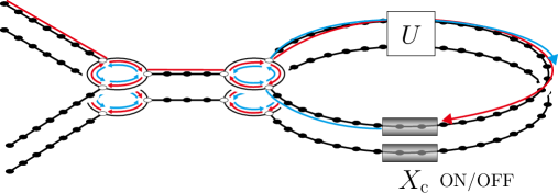
Figure 9: An example of a circuit that serves as a quantum memory. Information can be stored and retrieved at will by switching on the Pauli X gates installed on the loop. Iterative calculations can also be easily carried out by simply placing unitary gates on the loop, which may be helpful to perform, for instance, the Grover algorithm.

Appendix A Single- and two-particle scattering

In this appendix, to make our paper self-contained, we summarize single- and two-particle scattering states of indistinguishable quantum walkers.

A.1 Single-particle scattering on a graph

First, we consider the single-particle scattering on the graph $G$ defined in Fig. 3, using the procedure introduced in [23, 36]. Since the color of a single walker does not change (see (2.11)), the single-particle scattering can be considered independently in the case of a red walker and a blue walker. Therefore, first, we fix the color of the walker to red ($c=0$) (correspondingly, we only consider the part of $c=0$ in the kinetic term (2.11)), and omit the internal state $|0\rangle_{\mathrm{c}}$ to simplicity the notation. Later we will show that the single-particle $S$-matrix of the blue walker is nothing but the transpose of that for the red walker.

Consider the process in which an incident walker (wave packet) with a momentum near a specific value of $k\in(-\pi,0)$ passes through the $j$th semi-infinite path toward the graph $\hat{G}$ and exits to some semi-infinite paths $l$ (in superposition) after scattering from $\hat{G}$. Since an arbitrary wave packet is given by the superposition of plane waves of momentum close to $k$ as in (2.16), the scattering state $|\varphi_{j}(k)\rangle$ with a definite $k$ gives us information about how the wave packet scatters from $\hat{G}$. It is generally written as

$$|\varphi_{j}(k)\rangle=\sum_{x=0}^{\infty}e^{-ikx}|x,j\rangle+\sum_{l=0}^{N-1}\sum_{x=0}^{\infty}S_{lj}(k)e^{ikx}|x,l\rangle+\sum_{x\in V(\hat{G})\setminus T}\psi_{j}(x;k)|x\rangle,$$ (A.1)

where $|x,j\rangle$ denotes a walker at $x$ on the $j$th semi-infinite path (i.e. the walker at $(x,j)$), $V(\hat{G})\setminus T$ is the set of the $M$ internal vertices of $\hat{G}$, $S_{lj}(k)\in\mathbb{C}$ is the element of the $S$-matrix, and $\psi_{j}(x;k)\in\mathbb{C}$ is the wave-function on $\hat{G}$, which can be determined by the Schrödinger equation

$$\langle x|\mathcal{K}_{G}|\varphi_{j}(k)\rangle=E(k)\langle x|\varphi_{j}(k)\rangle\quad(x\in V(G)).$$ (A.2)

Here, $\mathcal{K}_{G}$ is the kinetic term defined as (2.11). Note that the interaction term (2.15) does not contribute to the single-particle scattering, and the color of the walker is implicitly assumed to be red ($|0\rangle_{\mathrm{c}}$) as explained above. In particular, for $(x,l)$ ($x\geq 1$), we have

$$\langle x,l|\mathcal{K}_{G}|\varphi_{j}(k)\rangle=2\cos k\langle x,l|\varphi_{j}(k)\rangle,\quad\langle x,l|\varphi_{j}(k)\rangle=e^{-ikx}\delta_{l,j}+e^{ikx}S_{lj}(k),$$ (A.3)

which determines the energy $E(k)$:

$$E(k)=2\cos k.$$ (A.4)

On the other hand, the Schrödinger equation (A.2) for $x\in\hat{G}$ is written as

$$\begin{pmatrix}A&B^{\dagger}\\ B&D\end{pmatrix}\binom{I_{N}+S(k)}{\psi(k)}+\binom{e^{-ik}I_{N}+e^{ik}S(k)}{0}=E(k)\binom{I_{N}+S(k)}{\psi(k)},$$ (A.5)

where

$$S(k):=\sum_{l=0}^{N-1}\sum_{j=0}^{N-1}S_{lj}(k)|0,l\rangle\langle 0,j|\in\operatorname{End}(\mathbb{C}^{N}),$$

$$\psi(k):=\sum_{x\in V(\hat{G})\setminus T}\sum_{j=0}^{N-1}\psi_{j}(x;k)|x\rangle\langle 0,j|\in\operatorname{Hom}(\mathbb{C}^{N},\mathbb{C}^{M}),$$ (A.6)

and the matrix consisting of $A\in\operatorname{End}(\mathbb{C}^{N})$, $D\in\operatorname{End}(\mathbb{C}^{M})$, and $B\in\operatorname{Hom}(\mathbb{C}^{N},\mathbb{C}^{M})$ is the adjacency matrix $\mathcal{A}(\hat{G})$: $A=A^{\dagger}$ and $D=D^{\dagger}$ are the adjacency matrices of the $N$ terminal vertices and the $M$ internal vertices, respectively, and $B$ is the adjacency matrix between the terminal and the internal vertices. Solving (A.5), one straightforwardly finds

$$S(k)=-e^{2ik}Q^{-1}(k)Q(-k),\quad Q(k):=\left\{1-e^{ik}\left(A+B^{\dagger}\frac{1}{2\cos k-D}B\right)\right\}.$$ (A.7)

For $k\in\mathbb{R}$, the $S$-matrix satisfies

$$S(k)^{\dagger}S(k)=S(-k)S(k)=1\quad(k\in\mathbb{R}),$$ (A.8)

which can be easily seen by noting that $A$ and $D$ are Hermitian, $Q(k)^{\dagger}=Q(-k)$, and $[Q(k),Q(-k)]=0$.

Finally, let us show that the single-particle $S$-matrix of the blue walker ($c=1$) (denote it by $\tilde{S}(k)$) is given by $\tilde{S}(k)=S(k)^{\mathrm{T}}$ for $k\in\mathbb{R}$, which is the transpose of the $S$-matrix of the red walker. By property (2.14), $\tilde{S}(k)$ can be obtained by simply replacing $\mathcal{A}(\hat{G})$ with $\mathcal{A}(\hat{G})^{\ast}$. More explicitly, it is given by replacing $\{A,B,D\}$ with $\{A^{\ast},B^{\ast},D^{\ast}\}$ in (A.7). This replacement changes $S(k)$ to $S(-k)^{\ast}$ ($k\in\mathbb{R}$). Using $S(k)^{\dagger}=S(-k)$ ($k\in\mathbb{R}$) derived from (A.8), we arrive at

$$\tilde{S}(k)=S(-k)^{\ast}=(S(k)^{\dagger})^{\ast}=S(k)^{\mathrm{T}}.$$ (A.9)

A.2 Two-particle scattering on an infinite path

Next, we consider the two-particle scattering on an infinite path: the walker (wave packet) with a momentum close to a specific value of $k_{0}\in(-\pi,0)$ moves right (down) toward the walker which moves left (up) with a momentum close to $k_{1}\in(0,\pi)$. Since, in our architecture, we are concerned with the scattering of red walkers, here, we only consider the spatial part of the states as in the single-particle scattering. The two-particle scattering process can be characterized by the scattering state $|\psi(k_{0},k_{1})\rangle$ with definite values of $(k_{0},k_{1})$. More explicitly,

$$|\psi(k_{0},k_{1})\rangle=\sum_{x_{0},x_{1}\in\mathbb{Z}}\psi(x_{0},x_{1};k_{0},k_{1})|x_{0},x_{1}\rangle,$$ (A.10)

where $x_{0},x_{1}\in\mathbb{Z}$ are vertices on an infinite path and the wave function $\psi(x_{0},x_{1};k_{0},k_{1})$ is written as

$$\psi(x_{0},x_{1};k_{0},k_{1})=\begin{dcases}e^{ik_{0}x_{0}+ik_{1}x_{1}}\pm S_{01}(k_{0},k_{1})e^{ik_{1}x_{0}+ik_{0}x_{1}}\,\,&(x_{0}<x_{1})\\ S_{01}(k_{0},k_{1})e^{ik_{0}x_{0}+ik_{1}x_{1}}\pm e^{ik_{1}x_{0}+ik_{0}x_{1}}\,\,&(x_{0}>x_{1})\end{dcases}.$$ (A.11)

$S_{01}\in\mathbb{C}$ is the scattering amplitude and the $+/-$ sign corresponds to bosons/fermions. For the bosonic case, $\psi(x,x)$ is given by putting formally $x_{0}=x_{1}=x$ in the above equation.

The form of the wave function (A.11) is followed by the following facts:

1. The individual momenta $k_{0}$ and $k_{1}$ are conserved after the scattering, due to the conservation law of the total energy $2(\cos k_{0}+\cos k_{1})$ and momentum $k_{0}+k_{1}$. The two walkers only acquire a phase factor $S_{01}(k_{0},k_{1})$ after the scattering.

2. The wave function is symmetric/antisymmetric under particle exchange, reflecting the Bose/Fermi statistics.

3. Interactions are limited to on-site or nearest-neighbor pairs.

Indeed, for $x_{0}\neq x_{1}$ (resp. $x_{0}\neq x_{1}+1$) in the bosonic (resp. fermionic) case, one can easily check that the wave function (A.11) satisfies the Schrödinger equation

$$\langle x_{0},x_{1}|\mathcal{H}_{G}|\psi(k_{0},k_{1})\rangle=2(\cos k_{0}+\cos k_{1})\psi(x_{0},x_{1};k_{0},k_{1}),$$ (A.12)

where $\mathcal{H}_{G}$ (eq. (2.10)) with the interaction term (2.15) is defined on an infinite path, i.e., $\theta_{jk}=0$. Below, solving (A.12) at $x_{0}=x_{1}$ (resp. $x_{0}=x_{1}-1$) for the bosonic (resp. fermionic) case, we determine the scattering amplitude $S_{01}(k_{0},k_{1})$.

A.2.1 Bosonic walkers

We adopt the on-site (Bose-Hubbard) interaction (2.15) for the bosonic quantum walkers. The LHS of the Schrödinger equation (A.12) at $x_{0}=x_{1}=:x$ gives

LHS $$=\psi(x,x+1;k_{0},k_{1})+\psi(x-1,x;k_{0},k_{1})$$

$$\quad+\psi(x,x-1;k_{0},k_{1})+\psi(x+1,x;k_{0},k_{1})+u\psi(x,x;k_{0},k_{1})$$

$$=\left[2(e^{ik_{1}}+e^{-ik_{0}})+u+S_{01}(k_{0},k_{1})\left\{2(e^{ik_{0}}+e^{-ik_{1}})+u\right\}\right]e^{i(k_{0}+k_{1})x}.$$ (A.13)

Because the RHS of (A.12) is given by

$$\text{RHS}=2(\cos k_{0}+\cos k_{1})(1+S_{01}(k_{0},k_{1}))e^{i(k_{0}+k_{1})x},$$ (A.14)

we arrive at

$$S_{01}(k_{0},k_{1})=\frac{2(\sin k_{0}-\sin k_{1})+iu}{2(\sin k_{0}-\sin k_{1})-iu}.$$ (A.15)

A.2.2 Fermionic walkers

For the fermionic quantum walkers, we employ the nearest-neighbor interaction (2.15). The LHS of the Schrödinger equation (A.12) at $x_{0}=x_{1}-1=:x$ gives

LHS $$=\psi(x-1,x+1;k_{0},k_{1})+\psi(x,x+2;k_{0},k_{1})+u\psi(x,x+1;k_{0},k_{1})$$

$$=\left[(e^{ik_{1}}+e^{-ik_{0}}+u)e^{ik_{1}}-S_{01}(k_{0},k_{1})\left\{(e^{ik_{0}}+e^{-ik_{1}}+u)e^{ik_{0}}\right\}\right]e^{i(k_{0}+k_{1})x}.$$ (A.16)

Also, we find the RHS of (A.12) is given by

$$\text{RHS}=2(\cos k_{0}+\cos k_{1})\left\{e^{ik_{1}}-S_{01}(k_{0},k_{1})e^{ik_{0}}\right\}e^{i(k_{0}+k_{1})x},$$ (A.17)

and therefore

$$S_{01}(k_{0},k_{1})=\frac{1+e^{i(k_{0}+k_{1})}-e^{ik_{1}}u}{1+e^{i(k_{0}+k_{1})}-e^{ik_{0}}u}.$$ (A.18)

References

- Konno [2002] Norio Konno. Quantum random walks in one dimension. Quantum Information Processing, 1(5):345–354, 2002.
- Kempe [2003] Julia Kempe. Quantum random walks: an introductory overview. Contemporary Physics, 44(4):307–327, 2003.
- Ambainis [2003] Andris Ambainis. Quantum walks and their algorithmic applications. International Journal of Quantum Information, 1(04):507–518, 2003.
- Kendon [2007] Viv Kendon. Decoherence in quantum walks–a review. Mathematical Structures in Computer Science, 17(6):1169–1220, 2007.
- Konno [2008] Norie Konno. Quantum walks. In Quantum potential theory, pages 309–452. Springer, 2008.
- Venegas-Andraca [2008] Salvador Elias Venegas-Andraca. Quantum walks for computer scientists. Synthesis Lectures on Quantum Computing, 1(1):1–119, 2008.
- Venegas-Andraca [2012] Salvador Elías Venegas-Andraca. Quantum walks: a comprehensive review. Quantum Information Processing, 11(5):1015–1106, 2012.
- Wang and Manouchehri [2013] Jingbo Wang and Kia Manouchehri. Physical implementation of quantum walks. Springer, 2013.
- Portugal [2013] Renato Portugal. Quantum walks and search algorithms. Springer, 2013.
- Moore and Russell [2002] Cristopher Moore and Alexander Russell. Quantum walks on the hypercube. In International Workshop on Randomization and Approximation Techniques in Computer Science, pages 164–178. Springer, 2002.
- Shenvi et al. [2003] Neil Shenvi, Julia Kempe, and K Birgitta Whaley. Quantum random-walk search algorithm. Physical Review A, 67(5):052307, 2003.
- Carneiro et al. [2005] Ivens Carneiro, Meng Loo, Xibai Xu, Mathieu Girerd, Viv Kendon, and Peter L Knight. Entanglement in coined quantum walks on regular graphs. New Journal of Physics, 7(1):156, 2005.
- Childs et al. [2003] Andrew M Childs, Richard Cleve, Enrico Deotto, Edward Farhi, Sam Gutmann, and Daniel A Spielman. Exponential algorithmic speedup by a quantum walk. In Proceedings of the thirty-fifth annual ACM symposium on Theory of computing, pages 59–68, 2003.
- Tregenna et al. [2003] Ben Tregenna, Will Flanagan, Rik Maile, and Viv Kendon. Controlling discrete quantum walks: coins and initial states. New Journal of Physics, 5(1):83, 2003.
- Ambainis [2007] Andris Ambainis. Quantum walk algorithm for element distinctness. SIAM Journal on Computing, 37(1):210–239, 2007.
- Richter [2007] Peter C Richter. Almost uniform sampling via quantum walks. New Journal of Physics, 9(3):72, 2007.
- [17] H Gerhardt and J Watrous. Random’03: Proceedings of the 7th international workshop on randomization and approximation techniques in computer science, princeton. Lecture Notes in Computer Science, 2764:290–301.
- Shiau et al. [2003] Shiue-yuan Shiau, Robert Joynt, and Susan N Coppersmith. Physically-motivated dynamical algorithms for the graph isomorphism problem. arXiv preprint quant-ph/0312170, 2003.
- Douglas and Wang [2008] Brendan L Douglas and Jingbo B Wang. A classical approach to the graph isomorphism problem using quantum walks. Journal of Physics A: Mathematical and Theoretical, 41(7):075303, 2008.
- Gamble et al. [2010] John King Gamble, Mark Friesen, Dong Zhou, Robert Joynt, and SN Coppersmith. Two-particle quantum walks applied to the graph isomorphism problem. Physical Review A, 81(5):052313, 2010.
- Berry and Wang [2011] Scott D Berry and Jingbo B Wang. Two-particle quantum walks: Entanglement and graph isomorphism testing. Physical Review A, 83(4):042317, 2011.
- Childs [2009] Andrew M Childs. Universal computation by quantum walk. Physical review letters, 102(18):180501, 2009. doi: http://dx.doi.org/10.1103/PhysRevLett.102.180501.
- Childs et al. [2013] Andrew M Childs, David Gosset, and Zak Webb. Universal computation by multiparticle quantum walk. Science, 339(6121):791–794, 2013. doi: https://doi.org/10.1126/science.1229957.
- Lovett et al. [2010] Neil B Lovett, Sally Cooper, Matthew Everitt, Matthew Trevers, and Viv Kendon. Universal quantum computation using the discrete-time quantum walk. Physical Review A, 81(4):042330, 2010.
- Underwood and Feder [2010] Michael S Underwood and David L Feder. Universal quantum computation by discontinuous quantum walk. Physical Review A, 82(4):042304, 2010.
- Reitzner et al. [2012] Daniel Reitzner, Daniel Nagaj, and Vladimir Buzek. Quantum walks. arXiv preprint arXiv:1207.7283, 2012.
- Bao et al. [2015] Ning Bao, Patrick Hayden, Grant Salton, and Nathaniel Thomas. Universal quantum computation by scattering in the fermi–hubbard model. New Journal of Physics, 17(9):093028, 2015.
- Thompson et al. [2016] KF Thompson, Can Gokler, Seth Lloyd, and Peter W Shor. Time independent universal computing with spin chains: quantum plinko machine. New Journal of Physics, 18(7):073044, 2016.
- Piccinini et al. [2017] Enrico Piccinini, Claudia Benedetti, Ilaria Siloi, Matteo GA Paris, and Paolo Bordone. Gpu-accelerated algorithms for many-particle continuous-time quantum walks. Computer Physics Communications, 215:235–245, 2017.
- Ezawa [2019] Motohiko Ezawa. Electric-circuit simulation of the schrödinger equation and non-hermitian quantum walks. Physical Review B, 100(16):165419, 2019.
- Tamura et al. [2020] Masaya Tamura, Takashi Mukaiyama, and Kenji Toyoda. Quantum walks of a phonon in trapped ions. Physical Review Letters, 124(20):200501, 2020.
- Ezawa [2020] Motohiko Ezawa. Electric circuits for universal quantum gates and quantum fourier transformation. Physical Review Research, 2(2):023278, 2020.
- Singh et al. [2021] Shivani Singh, Prateek Chawla, Anupam Sarkar, and CM Chandrashekar. Universal quantum computing using single-particle discrete-time quantum walk. Scientific Reports, 11(1):1–13, 2021.
- Asaka et al. [2021] Ryo Asaka, Kazumitsu Sakai, and Ryoko Yahagi. Quantum random access memory via quantum walk. Quantum Science and Technology, 6(3):035004, 2021. doi: https://doi.org/10.1088/2058-9565/abf484.
- Asaka et al. [2022] Ryo Asaka, Kazumitsu Sakai, and Ryoko Yahagi. Two-level quantum walkers on directed graphs II: An application to qRAM. arXiv preprint arXiv:2204.08709, 2022.
- Childs and Gosset [2012] Andrew M Childs and David Gosset. Levinson’s theorem for graphs II. Journal of Mathematical Physics, 53(10):102207, 2012. doi: https://doi.org/10.1063/1.4757665.
- Aharonov and Casher [1984] Yakir Aharonov and Aharon Casher. Topological quantum effects for neutral particles. Physical Review Letters, 53(4):319, 1984.
- Zvyagin and Krive [1992] AA Zvyagin and IV Krive. Aharonov-casher effect in the hubbard model with repulsion. Soviet physics, JETP, 75(4):745–747, 1992.
- Nielsen and Chuang [2002] Michael A Nielsen and Isaac Chuang. Quantum computation and quantum information, 2002.
- Williams [2011] Colin P Williams. Quantum gates. In Explorations in Quantum Computing, pages 51–122. Springer, 2011.
- Farhi et al. [2007] Edward Farhi, Jeffrey Goldstone, and Sam Gutmann. A quantum algorithm for the hamiltonian nand tree. arXiv preprint quant-ph/0702144, 2007.
- Grover [1996] Lov K Grover. A fast quantum mechanical algorithm for database search. In Proceedings of the twenty-eighth annual ACM symposium on Theory of computing, pages 212–219, 1996.
- Shor [1994] Peter W Shor. Algorithms for quantum computation: discrete logarithms and factoring. In Proceedings 35th annual symposium on foundations of computer science, pages 124–134. Ieee, 1994.
- Asaka et al. [2020] Ryo Asaka, Kazumitsu Sakai, and Ryoko Yahagi. Quantum circuit for the fast fourier transform. Quantum Information Processing, 19(8):1–20, 2020.