Testing Instrument Validity with Covariates

Abstract

We develop a novel test of the instrumental variable identifying assumptions for heterogeneous treatment effect models with conditioning covariates. We assume semiparametric dependence between potential outcomes and conditioning covariates. This allows us to obtain testable equality and inequality restrictions among the subdensities of estimable partial residuals. We propose jointly testing these restrictions. To improve power, we introduce distillation, where a trimmed sample is used to test the inequality restrictions. In Monte Carlo exercises we find gains in finite sample power from testing restrictions jointly and distillation. We apply our test procedure to three instruments and reject the null for one.

Keywords: Program evaluation, local average treatment effect, marginal treatment effect.

1 Introduction

Instrumental variable (IV) methods are widely used in empirical economics. The credibility of IV estimates relies on the validity of the identifying assumptions, which are often subject to debate. In IV estimation, conditioning covariates are frequently used to enhance the credibility of the identifying assumptions or improve the precision of estimates. For example, when using proximity to college as an instrument to estimate the return to schooling, researchers control for location characteristics which may otherwise induce dependence between the instrument and the outcome. Huber and Mellace (2015), Kitagawa (2015), and Mourifié and Wan (2017) propose statistical tests for instrument validity in the heterogeneous treatment effect model of Imbens and Angrist (1994). However, the state of the art literature lacks high-power tests for instrument validity that remain computationally feasible for more than a small number of covariates.

The first contribution of this paper is to propose an easy-to-implement test procedure for instrumental validity in the heterogeneous treatment effect model that can accommodate a moderate to large number of conditioning covariates. Building on the semiparametric approach of Carneiro et al. (2011), we specify that conditioning covariates are independent of unobserved hetergoneity and affect potential outcomes linearly. Under these restrictions, the conditional expectation of the outcome given conditioning covaraites and the instrument follows a partially linear model that depends non-parametrically on the probability of receiving treatment (propensity score). This allows the conditioning covariates to be partialed out and partial residuals obtained. Testable implications for the instrumental variable identifying assumptions which hold without conditioning on covariates can be stated for the subdensities of these partial residuals. With partial residuals in hand, testing can be performed without reference to covariate values. In comparison to the test procedure with conditioning covariates proposed in Kitagawa (2015), this greatly reduces the computational burden. Increasing the number of conditioning covariates increases only the complexity of estimating the propensity score and partially linear model, not the number of implications to be tested.

Two testable implications are available: index sufficiency and nesting inequalities. Index sufficiency states that the partial residual subdensities depend on the instrument through the propensity score only. The nesting inequalities are monotonicity inequalities for the joint distributions of the partial residuals and treatment status. They state that, for two distinct values of the propensity score, the distribution of partial residuals for treated units with the higher propensity score nests that of units with the lower propensity score, and the converse is true for untreated units. The two testable implications complement each other: index sufficiency holds the propensity score fixed and compares subdensities for different values of the instrument, while the nesting inequalities compare subdensities for different propensity scores. To exploit this complementarity, we propose jointly testing the two.

As the subdensity nesting inequalities are ordered with respect to the propensity score, a natural approach to testing them would be to coarsen the propensity score and test the monotonicity of the subdensities conditional on this coarsened propensity score. When the propensity score is strongly correlated with the conditioning covariates, this approach can result in a test with low power. In such cases, classifying observations by propensity score will homogenise the distribution of instrument values across propensity score bins, which can mask violations of instrument validity.

Our second contribution is to propose a novel approach to testing the nesting inequalities. We suggest testing instead monotonicity of the conditional partial residual subdensities given the instrument. This approach ensures that observations with different instrument values are kept separate. We show that, when the identifying assumptions are satisfied, the nesting inequalities hold over instrument values if the conditional distribution of propensity scores is monotonic in the instrument in the sense of first-order stochastic dominance. If first-order stochastic dominance does not hold for the instrument, we propose trimming the sample and testing the nesting inequalities for a sub-sample where first-order stochastic dominance is satisfied. We refer to this process as distillation as it distills the sample down to the observations best able to detect violations.

We show analytically and numerically the benefits of implementing distillation in terms of the ability to detect violation of instrument validity conditional on covariates. Specifically, we present a class of data generating processes for which distillation dominates conditioning on the coarsened propensity score in the following sense. A violation of the nesting inequalities conditional on the coarsened propensity score implies a larger violation of the nesting inequalities with a distilled sample, but not vice versa. That is, a violation of the nesting inequalities with a distilled sample does not imply the existence of a violation of the nesting inequalities conditional on the coarsened propensity score. Consequently, there exist data generating processes where instrument validity fails but the violation can only be detected by the nesting inequalities when performing distillation.

We perform Monte Carlo exercises to evaluate the size and power of the proposed test procedure and compare it to two alternatives: the Kitagawa (2015) test that does not control for covariates, and the test of nesting inequalities using a coarsened propensity score. We consider processes where the instrument is independent of the covariates, and processes where it is not. In the first case, an instrument that is valid conditional on the covariates will also be valid without conditioning on covariates, so the size of the Kitagawa (2015) test will not be distorted. In the second, size will only be controlled if the conditioning covariates are appropriately controlled for. We find that the size of the proposed test is controlled in all cases. For processes where the Kitagawa (2015) test has the correct size, we find our test procedure has comparable power. For all processes, it has higher power than the test of nesting inequalities using a coarsened propensity score. We also investigate the contributions of the index sufficiency and nesting inequality tests to the power of the joint test. These results suggest that index sufficiency has most power when the distributions of propensity scores for different instrument values are similar, so that there are observations with different instrument values and a similar propensity score. On the other hand, for the processes considered, rejection probabilities when testing the nesting inequalities do not depend strongly on the similarity of the propensity score distributions across instrument values. This is consistent with the two testable implications being complementary.

To demonstrate the feasbility of the test procedure and illustrate how it can be used to resolve questions of instrument credibility, we present three applications. The first is Card (1993). This instrument has been tested in Huber and Mellace (2015), Kitagawa (2015), Mourifié and Wan (2017) and Sun (2021) but, for computational reasons, in each case only a subset of the conditioning covariates of the original specification is used. The proposed test procedure allows all conditioning covariates to be included and remains computationally feasibile. Second, we apply the test to the same-sex instrument of Angrist and Evans (1998). The validity of this instrument was been questioned in Rosenzweig and Wolpin (2000) and its validity has been formally tested by Huber (2015) and Mourifié and Wan (2017). As with Card (1993), these studies use only a subset of the conditioning covariates, while our test procedure allows us to include all conditioning covariates. Finally, we turn to identifying strategies that rely on geographical variation in the timing of changes in compulsory schooling laws. Using data for America, Stephens and Yang (2014) presents evidence that changes in education laws are correlated with other unobserved state-level changes, which suggests that this instrument is not valid. We test its validity in the case of the UK using the data of Oreopoulos (2006).

The remainder of the paper proceeds as follows. The related literature is reviewed in Section 1.1 below. Section 2 introduces the semiparametric testable implications. Section 3 describes the test procedure. Section 4 presents Monte Carlo exercises. Section 5 discusses our three empirical applications. Section 6 concludes.

1.1 Related Literature

This paper contributes to the active literature on the identification and estimation of the local average treatment effect (LATE) model of Angrist et al. (1996) and Imbens and Angrist (1994) and the marginal treatment effect model (MTE) of Heckman and Vytlacil (1999, 2001a, 2001b, 2005). This literature has recently been reviewed by Mogstad and Torgovitsky (2018). A testable implication of the LATE identifying restrictions was derived in Balke and Pearl (1997), Imbens and Rubin (1997) and Heckman and Vytlacil (2005). Kitagawa (2015) shows that this testable implication is sharp, and proposes a test procedure using a Kolmogorov-Smirnov statistic. Mourifié and Wan (2017) reformulates this testable implication as a conditional moment inequality, and proposes a test based on the intersection bounds framework of Chernozhukov et al. (2013). It is straightforward to generalise this testable implication to incorporate conditioning covariates, but assessing it nonparametrically in a finite sample is limited by the capacity of nonparametric methods to handle multiple conditioning covariates.

To facilitate the estimation of marginal treatment effects while controlling for multiple conditioning covariates, Carneiro et al. (2011) further imposes that potential outcomes are linear in the conditioning covariates, unobserved heterogeneities enter additively, and these unobservables are statistically independent of the covariates and instrument. The test procedure presented in this paper corresponds to a test for the validity of the Carneiro et al. (2011) identifying assumptions. Maestas et al. (2013), Eisenhauer et al. (2015), Kline and Walters (2016), Cornelissen et al. (2018), Felfe and Lalive (2018), Bhuller et al. (2020), and Coury et al. (2022) among others apply the approach of Carneiro et al. (2011) to recover marginal treatment effects. Our test procedure can be applied in any of these contexts to assess the validity of the identifying assumptions. Furthermore, even if the validity of the instrument is undisputed, the test procedure can still be used to detect errors in the functional form specification for the relationship between potential outcomes and conditioning covariates. Brinch et al. (2017) further develops the approach of Carneiro et al. (2011), and show how marginal treatment effects can be identified in a variety of settings. Mogstad et al. (2018) discusses how to extrapolate marginal treatment effects to set identify policy relevant treatment effects.

Several alternative tests of the LATE identifying assumptions have been proposed. Huber and Mellace (2015) considers a weaker set of identifying restrictions than Kitagawa (2015), derives a testable implication, and proposes several test procedures. Laffers and Mellace (2017) shows that the testable implication of Huber and Mellace (2015) is sharp for these identifying assumptions. Sun (2021) derives testable implications when the treatment is an ordered or unordered multi-valued variable, and proposes a power improving refinement of the Kitagawa (2015) test procedure. Arai et al. (2022) extends the Kitagawa (2015) test to fuzzy regression discontinuity designs. Farbmacher et al. (2022) proposes a test procedure that uses random forests and classification and regression trees to find violations of the monotonicity and exclusion assumptions. Kédagni and Mourifié (2020) derives a testable implication of the instrument independence assumption in the form of a set of inequalities, reformulates these inequalities as a set of conditional expectations, and develops a test procedure using the framework of Chernozhukov et al. (2013). Machado et al. (2019) discusses tests for instrument validity in the case of a binary outcome which responds monotonically with respect to the treatment. Frandsen et al. (2023) develops a test of the identifying assumptions of research designs which exploit random assignment of judges. The closest paper to ours is Mao and Sant’Anna (2020), which also uses the MTE framework of Carneiro et al. (2011), and derives index sufficiency and the nesting inequalities. This paper focuses on testing the nesting inequalities, and does not jointly test index sufficiency. The nesting inequalities are tested by considering many possible discretisations of the propensity score. We differ in that we jointly test index sufficiency and the nesting inequalities. In addition, for the nesting inequalities, rather than examining subdensities indexed by the propensity score, we propose constructing a distilled sample so that the inequalities hold for subdensities indexed by the instrument, and show the advantages of this approach.

We contribute to several empirical literatures by testing the validity of commonly used instruments and identification strategies. The college proximity instrument of Card (1993) has also been employed in Cameron and Taber (2004) to estimate the effects of borrowing constraints on education, Carneiro et al. (2011) to estimate the marginal treatment effect of education, and Heckman et al. (2018) to estimate the effects of education on labour market and health outcomes. The same-sex instrument of Angrist and Evans (1998) has been used widely to identify the effects of family size. Black et al. (2010),Conley and Glauber (2006), Angrist et al. (2010) and Becker et al. (2010) use this instrument to empirically investigate the existence of a quantity-quality trade-off for children, while Cruces and Galiani (2007) employs it to investigate the relationship between family size and maternal labour supply. Other than Oreopoulos (2006), geographical variation in schooling laws has been employed by Acemoglu and Angrist (2000) to estimate human capital externalities, Lochner and Moretti (2004) to estimate the effect of education on imprisonment rate, and Clark and Royer (2013) to estimate the effects of education on life expectancy.

2 Model and Testable Implications

2.1 Setting

The data is a random sample $\left(Y,D,X,Z\right)$, where $Y$ is an observed outcome continuously distributed on $\mathbb{R}$, $D\in\left\{1,0\right\}$ is an observed binary treatment status indicating treated $(D=1)$ or non-treated $\left(D=0\right)$, $X\in\mathcal{X}\subset\mathbb{R}^{k_{X}}$ is a vector of individual pretreatment observable covariates, and $Z\in\mathcal{Z}\subset\mathbb{R}^{k_{Z}}$ is a vector of instrumental variables. For the moment, we impose no restrictions on the instrument.  Let $\left\{Y_{dz}\right\}_{d\in\left\{1,0\right\},z\in\mathcal{Z}}$ be the set of potential outcomes indexed by treatment status $d\in\left\{1,0\right\}$ and instrument value $z\in\mathcal{Z}$. The observed outcome $Y$ can be written as

$$Y=Y_{1Z}D+Y_{0Z}(1-D)\text{.}$$

We write a selection equation of unconstrained form as

$$D=1\{v(X,Z,U_{D})\geq 0\}.$$

We interpret this selection equation as follows. With $U_{D}$ fixed at $u_{D}$, $D_{xz}=1\{v(x,z,u_{D})\geq 0\}$ generates the counterfactual selection response for an individual when their pre-treatment characteristics $X$ and instrument $Z$ are exogenously set at $x$ and $z$.

The following three assumptions identify the marginal treatment effect (MTE):

MTE Identification Assumptions (Heckman and Vytlacil (2005)):

(A1)

Instrument exclusion restriction: Potential outcomes do not depend on the instrument in the sense $Y_{1z}=Y_{1}$ and $Y_{0z}=Y_{0}$ for all $z\in\mathcal{Z}$ with probability one.

(A2)

Random assingnment: $(\left\{Y_{1z}\right\}_{z\in\mathcal{Z}},\left\{Y_{0z}\right\}_{z\in\mathcal{Z}},U_{D})$ are statistically independent of $Z$ conditional on $X$, and $U_{D}$ is statistically independent of $X$.

(A3)

Instrument monotonicity: For every $z$, $z^{\prime}\in\mathcal{Z}$, $v(x,z,u_{D})\geq v(x,z^{\prime},u_{D})$ holds for all $u_{D}\in\mathcal{U}$ or $v(x,z,u_{D})\leq v(x,z^{\prime},u_{D})$ holds for all $u_{D}\in\mathcal{U}$.

The instrument exclusion restriction (A1) precludes the instrument from having a direct causal impact on the outcome for any member of the population. With this restriction imposed, an individual’s potential outcomes are reduced to a pair indexed only by their treatment status, i.e, $Y_{1}$ denotes their potential outcome with treatment and $Y_{0}$ their potential outcome without treatment. The observed outcome $Y$ can then be written as $Y=Y_{1}D+Y_{0}(1-D)$.

Assumption (A2) states that, conditional on $X$, the instrument $Z$ is assigned without reference to underlying potential outcomes and unobserved heterogeneity in selection response. This corresponds to the conventional assumption of instrument exogeneity. In the heterogeneous treatment effect model, however, it should be noted that instrument exogeneity takes the form of joint statistical independence of potential outcomes and selection heterogeneities, rather than the zero-correlation exogeneity restriction. Assumption (A3) states that a hypothetical change in the instrument from $z^{\prime}$ to $z$ can induce some individuals to opt in to treatment or some individuals to opt out of treatment, but never both simultaneously. Equivalently, in the terminology of Imbens and Angrist (1994), there is a sub-population of compliers associated with this hypothetical change, but no sub-population of defiers. Instrument monotonicity of the form (A3) allows for multiple instrumental variables. Mogstad et al. (2020) argue that, in the presence of multiple instruments, (A3) implies severe restrictions on individual selection responses. Our test procedure allows for multiple instruments and can be used to assess a necessary testable implication of (A3) jointly with the exclusion and random assignment restrictions. Section 3.2.3 discusses in detail the implications of multiple instruments for instrument validity testing.

Following Heckman and Vytlacil (2001a, 2005), assumptions (A1) - (A3) imply a heterogeneous treatment effect model of the following form:

$$\left\{\begin{array}[]{l}Y_{1}=m_{1}(X)+\tilde{U}_{1};\\ Y_{0}=m_{0}(X)+\tilde{U}_{0};\\ Y=DY_{1}+(1-D)Y_{0};\\ D=\mathbbm{1}\{p(X,Z)-V\geq 0\},\end{array}\right.$$ (1)

with

$$\left(Y_{1},Y_{0},V\right)\perp Z|X\text{ \ and }V\perp X.$$ (2)

Here, $E[Y_{1}|X=x]=m_{1}(x)$ and $E[Y_{0}|X=x]=m_{0}(x)$ are regression equations of potential outcomes $(Y_{1},Y_{0})$ on the control covariates, $\tilde{U}_{1}$ and $\tilde{U}_{0}$ are unobserved heterogeneities in the potential outcomes $(Y_{1},Y_{0})$, $p(x,z)=\Pr(D=1|X=x,Z=z)$ is the propensity score, and $V$ is uniformly distributed on $[0,1]$ and is independent of $(X,Z)$.

2.2 Semiparametric Testable Implications

The MTE identifying assumptions introduced above involve counterfactual variables that are never jointly observed for the same individual, so cannot be directly verified using the distribution of observables. However, necessary testable implications have been established. These conditions relate to the distribution of observables, so may be examined empirically. They consist of single index sufficiency and nesting inequalities. We present a proof in Appendix A for completeness.

Proposition 1

Assume (A1) - (A3) and that, conditional on $X=x$, the propensity score $p\left(X,Z\right)$ has a nondegenerate distribution.  Then, at any such $x$, the following two conditions hold:

(i) Index sufficiency: The conditional distribution of $(Y,D)$ given $(X,Z)$ depends on $Z$ only through the propensity score $p(X,Z)$, i.e., for any measurable set $A\subset\mathcal{Y}$ and $d\in\{0,1\}$,

$$\Pr(Y\in A,D=d|X=x,Z=z)=\Pr(Y\in A,D=d|p(X,Z)=p,X=x)$$ (3)

holds for any $(x,z)$ where $p=p(x,z)$.

(ii) Nesting inequalities: The following inequalities hold for every $p\geq p^{\prime}$ in the support of $p\left(X,Z\right)$ and every measurable subset $A\subset\mathcal{Y}$:

$$\Pr(Y\in A,D=1|p\left(X,Z\right)=p,X=x)\geq\Pr(Y\in A,D=1|p\left(X,Z\right)=p^{\prime},X=x),$$ (4)

$$\Pr(Y\in A,D=0|p\left(X,Z\right)=p,X=x)\leq\Pr(Y\in A,D=0|p\left(X,Z\right)=p^{\prime},X=x).$$

Condition (i), index sufficiency, restricts the conditional distribution of $(Y,D)$ given $(X,Z)$ to depend on $Z$ through the propensity score $p(X,Z)$ only. That is, if there are multiple values of $Z$, say $z\neq z^{\prime}\in\mathcal{Z}$, that yield the same value of the propensity score given $X=x$, the conditional distributions of $(Y,D)$ given $(X=x,Z=z)$ and $(X=x,Z=z^{\prime})$ must be identical. Condition (ii) provides distributional monotonicity inequalities among the conditional distributions of $(Y,D)$ given $(p,x)$ with respect to $p=p(X,Z)$. This corresponds to the testable monotonicity shown by Heckman and Vytlacil (2005). The difference between the two sides of (4) can be expressed as

$$\Pr(Y_{1}\in A,p^{\prime}<U_{D}\leq p|X=x)$$

$$= \Pr(Y_{1}\in A|p^{\prime}<U_{D}\leq p,X=x)\times\Pr\left(p^{\prime}<U_{D}\leq p|X=x\right).$$

Individuals whose selection heterogeneity $U_{D}$ falls in $(p^{\prime},p]$ can be viewed as compliers conditional on $X=x$. (4) imposes non-negativity of the treated outcome probability density function for these conditional compliers. Detecting any violation of the conditions of Proposition 1 allows the joint restrictions (A1) - (A3) to be refuted. Neither of these testable implications restrict the support of the instrument $Z$, i.e., $Z$ can be discrete, continuous, or multi-dimensional.

The two testable implications shown in Proposition 1 are distinct and assess different aspects of the distribution of observables. Holding $X$ fixed, index sufficiency compares conditional distributions of $(Y,D)$ given $(p(X,Z),X)$ at a fixed value of the propensity score, while the nesting inequalities compare conditional distributions across different values of the propensity score. Consequently, there are scenarios in which one testable implication is useful for assessing instrument validity but the other is not. For instance, if $Z$ is a scalar and $p(x,z)$ is strictly monotonic in $z$ at every $x$, instrument validity cannot be assessed through index sufficiency since their is no variation in the instrument conditional on $(p(X,Z),X)$, whereas it can be assessed using the nesting inequalities. Conversely, when the propensity score does not vary with the instrument conditional on $X$ (i.e. the instrument is irrelevant), index sufficiency does have content for assessing instrument validity while the nesting inequalities do not. As such, the two testable implications complement each other and joint assessment of them is desirable.

When the dimension of $X$ is not small, nonparametrically testing the implications listed in Proposition 1 is challenging. Kitagawa (2015) proposes testing the inequalities of Proposition 1 (ii) with a Kolmogorov-Smirnov type test statistic where a supremum is taken over a large class of instrument functions defined on the product space of $Y$ and $X$. Similar to optimization in the empirical risk minimizing classification problem, the computational complexity of searching for this supremum increases with the dimension of $X$. Due to this computational barrier, the finite sample power of this test is unknown, and it has rarely been implemented in practice. Furthermore, accommodating a continuous instrument in this procedure remains an open problem.

We develop a test for instrument validity which circumvents the implementation issues that arise due to conditioning covariates. This test jointly assesses index sufficiency and the nesting inequalities. In addition, the test procedure can accommodate continuous instruments.

To achieve this, we impose the semiparametric restrictions proposed by Carneiro et al. (2011), which have since been used in many empirical studies of marginal treatment effects.

(A4)

Linear Functional Form: The regression equations for potential outcomes have the parametric form

$$\left\{\begin{array}[]{c}Y_{1}=\alpha_{1}+X^{\prime}\theta_{1}+\tilde{U}_{1};\\ Y_{0}=\alpha_{0}+X^{\prime}\theta_{0}+\tilde{U}_{0},\end{array}\right.$$ (5)

In addition, strengthen the exogeneity restriction (A2) to:

(A5)

Strong Exogeneity: Let $(\tilde{U}_{1},\tilde{U}_{0})$ be the residuals of the potential outcome regression equations defined in (5). $(\tilde{U}_{1},\tilde{U}_{0},V)$ is independent of $\left(X,Z\right)$.

(A4) restricts the conditional mean potential outcomes to depend linearly on the covariates. (A5) implies that the mean zero unobserved terms $\left(\tilde{U}_{1},\tilde{U}_{0}\right)$ are independent of the covariates. (A4) and (A5) jointly imply that covariates affect the potential outcomes only through their conditional means. Note that this assumption does not imply that the treatment effect is homogeneous, since the individual causal effect $Y_{1}-Y_{0}$ remains random even conditional on $X$. Note also that, while only conditional mean treatment effects may depend on $X$, the distribution of treatment effects remains otherwise unconstrained.

In general, under (A1) - (A3), the MTE at $X=x$ and $V=p\in\mathcal{P}$ is nonparametrically identified by

$$\frac{\partial}{\partial p}E\left[Y|p\left(X,Z\right)=p,X=x\right].$$

Carneiro et al. (2011) shows that imposing the parametric functional forms of (A4) together with strengthening the exogeneity assumption of (A2) to (A5), yields the following partially linear regression equation for the observed outcome $Y$:

$$E\left[Y|p\left(X,Z\right)=p,X=x\right]=x^{\prime}\theta_{0}+px^{\prime}\left(\theta_{1}-\theta_{0}\right)+\phi\left(p\right)\text{,}$$ (6)

where $\phi\left(\cdot\right)$ is a unknown function of the propensity score, which absorbs the intercept term $p\alpha_{1}+\left(1-p\right)\alpha_{0}$. As a result, the MTE at $X=x$ and $V=p$ is identified by

$$MTE(x,p)\equiv E[Y_{1}-Y_{0}|X=x,V=p]=x^{\prime}\left(\theta_{1}-\theta_{0}\right)+\phi^{\prime}\left(p\right).$$ (7)

Since the only nonparametric component in this regression equation is $\phi\left(\cdot\right)$, which is a function of the scalar-valued propensity score, the computational complexity of estimation does not explode as the dimension of $X$ increases. Carneiro et al. (2011) argues that this is a practical advantage of the functional form specification (A4) and the stronger instrument exogeneity assumption (A5).

Since the partial linear regression (6) identifies $\left(\theta_{1},\theta_{0}\right)$, it is possible to compute

$$U_{1}\equiv\alpha_{1}+\tilde{U}_{1}=Y_{1}-X^{\prime}\theta_{1}$$

for every treated observation, and

$$U_{0}\equiv\alpha_{0}+\tilde{U}_{0}=Y_{0}-X^{\prime}\theta_{0}$$

for every untreated observation.

The joint restrictions (A1), (A3), (A4) and (A5) simplify not only estimation of MTE, but also the testable implications of MTE identifying assumption. To see how, consider the distribution of $U_{1}$ conditional on $\left(D=1,p\left(X,Z\right)=p,X=x\right)$.  Under (A1), (A3) and (A4),

$$U_{1}|\left(D=1,p\left(X,Z\right)=p,X=x\right) \sim U_{1}|\left(V\leq p,p\left(X,Z\right)=p,X=x\right)$$ (8)

$$\sim U_{1}|\left(V\leq p\right),$$

and similarly,

$$U_{0}|\left(D=0,p\left(X,Z\right)=p,X=x\right) \sim U_{0}|\left(V>p,p\left(X,Z\right)=p,X=x\right)$$ (9)

$$\sim U_{0}|\left(V>p\right).$$

That is, for $d=0,1$, the distribution of the residual, $U_{d}=Y_{d}-X^{\prime}\theta_{d}$, conditional on $\left(D=d,p\left(X,Z\right),X\right)$ depends only on $p\left(X,Z\right)$. Exploiting this single index sufficiency for the distributions of $U_{1}$ and $U_{0}$, we obtain the following necessary testable implications for the joint restrictions (A1), (A3), (A4) and (A5).

Proposition 2

Let $U=DU_{1}+(1-D)U_{0}$. Assume the propensity score $p\left(X,Z\right)$ has a nondegenerate distribution. If (A1), (A3), (A4) and (A5) hold, then the following two conditions hold:

(i) Index sufficiency: The conditional distribution of $(U,D)$ given $(X,Z)$ depends only on the propensity score $p(X,Z)$, i.e., for any measurable set $A\subset\mathbb{R}$ and $d\in\{0,1\}$

$$\Pr(U\in A,D=d|X=x,Z=z)=\Pr(U\in A,D=d|p(X,Z)=p)$$ (10)

holds for any $(x,z)$ where $p=p(x,z)$.

(ii) Nesting inequalities: For every $p\geq p^{\prime}$ in the support of the propensity score distribution and every measurable subset $A\subset\mathcal{Y}$:

$$\Pr(U\in A,D=1|p\left(X,Z\right)=p)\geq\Pr(U\in A,D=1|p\left(X,Z\right)=p^{\prime}),$$ (11)

$$\Pr(U\in A,D=0|p\left(X,Z\right)=p)\leq\Pr(U\in A,D=0|p\left(X,Z\right)=p^{\prime}).$$

We refer to the joint restrictions of (A1), (A3), (A4), and (A5) as instrument validity and base our test on the testable implications of Proposition 2. Compared to Proposition 1, Proposition 2 replaces the outcome variable $Y$ with the outcome residuals $U$, and removes the requirement to condition on $X$. Index sufficiency is strengthened such that the distribution of $(U,D)$ depends on $(X,Z)$ only through the propensity score $p(X,Z)$. The nesting inequalities are strengthened to imply distributional monotonicity with respect to changes in $p(X,Z)$ regardless of the underlying variation in $(X,Z)$. These testable implications are also shown in Mao and Sant’Anna (2020).

As the testable implications of Proposition 2 follow from assumptions (A1), (A3), (A4) and (A5), any test based on them is a joint test of these assumptions. That is, in addition to the conventional exclusion, random assignment and monotonicity, we will be testing the functional form assumption of (A4) and strong exogenienty assumption of (A5). Violation of testable implications can be due to misspecification in the functional form (5) or the restricted heterogeneity of MTEs with respect to the observable characteristics, i.e., additive separability of MTEs in (7). In addition, when the propensity score is estimated, misspecification of the propensity score function may also lead to a rejection of the null.

As index sufficiency should hold for all $(X,Z)$ it leads to a large number of inequalities, and testing all of them may be impractical. In this paper our focus is on testing the validity of the instrument, assuming that the strong exogeneity of $X$ holds. As such, we focus on testing that the conditional joint distribution of $(U,D)$ given the propensity score does not vary with $Z$.

2.3 Potential Difficulties Detecting Violation of Instrument Validity

In this section we show how the conditional distribution of the propensity score given $Z$ affects the usefulness of each of the testable implications characterized in Proposition 2. We use the simple case of a single binary instrument to illustrate this point.

Index sufficiency (10) can be tested by examining whether the difference

$$\Pr(U\in A,D=d|p(X,Z)=p,Z=1)-\Pr(U\in A,D=d|p(X,Z)=p,Z=0)$$ (12)

is zero.

For a data generating process to have empirical content to asses index sufficiency, there must exist some $p$ where observations with both $Z=0$ and $Z=1$ are available. This occurs if we can find covariate values $x\neq x^{\prime}$ such that $p(x,1)=p(x^{\prime},0)$. If no such $p$ exists, then for all $p$ either $\Pr(p(X,Z)=p,Z=0)=0$ or $\Pr(p(X,Z)=p,Z=1)=0$ and (12) cannot be calculated. Hence, the practical relevance of (10) is determined by the degree of overlap between the propensity score distributions conditional on $Z=0$ and $Z=1$.

Now consider the nesting inequalities (11). These can be viewed as analogous to those tested in Kitagawa (2015) with the observed outcome $Y$ replaced by the outcome residual $U$ and the instrument replaced by the propensity score $p(X,Z)$. If the propensity score were coarsened, e.g., by binning, the test procedure with no conditioning covariates and a discrete instrument of Kitagawa (2015) could be applied. Although this approach would attain an asymptotically valid test size, there are circumstances where conditioning on the propensity score has a detrimental effect on power.

Maintain the simplifying assumption of a single binary instrument. Assume that the conditioning covariates $X$ are statistically independent of the unobservables $(\tilde{U}_{1},\tilde{U}_{0},V)$,as required by (A5). Furthermore, assume that they are also independent of $Z$. Consider the following simple violation of the exclusion restriction (A1) where the residuals of the potential outcome regression for $D=1$ depend on $Z$

$$U_{1}=\alpha_{1}+\nu Z+\tilde{U}_{1},$$ (13)

with $\nu\neq 0$. As $U_{1}$ is a sum of quantities that are independent of $Z$, it will be independent of $Z$.

If $\Pr(Z=1|p(X,Z)=p)$ is bounded away from 0 and 1, the additive separability of the selection equation and the independence of $X$ leads to the following decomposition:

$$\Pr(U\in A,D=1|p(X,Z)=p)= \Pr(U\in A,D=1|p(X,Z)=p,Z=0)\Pr(Z=0|p(X,Z)=p)$$

$$+\Pr(U\in A,D=1|p(X,Z)=p,Z=1)\Pr(Z=1|p(X,Z)=p)$$

$$= \Pr(U_{1}\in A,V\leq p|p(X,Z)=p,Z=0)\Pr(Z=0|p(X,Z)=p)$$

$$+\Pr(U_{1}\in A,V\leq p|p(X,Z)=p,Z=1)\Pr(Z=1|p(X,Z)=p)$$

$$= \Pr(U_{1}\in A,V\leq p|Z=0)\Pr(Z=0|p(X,Z)=p)$$

$$+\Pr(U_{1}\in A,V\leq p|Z=1)\Pr(Z=1|p(X,Z)=p).$$ (14)

The first equality states that, for a given $p$ where $\Pr(Z=1|p(X,Z)=p)$ is bounded away from 0 and 1, we have a mixture of observations with $Z=0$ and $Z=1$ with conditioning covariates implicitly adjusting to hold the propensity score constant. The second equality uses that the event $(U\in A,D=1)$ is equivalent to $(U_{1}\in A,V\leq p)$. To see the third, note that conditioning on $(p(X,Z)=p,Z=z)$ is equivalent to conditioning on $Z=z$ and $X\in\{x|p(X=x,Z=z)=p\}$. $X$ is independent of $V$ and $U_{1}$, so $X\in\{x|p(X=x,Z=z)=p\}$ can be dropped from the conditioning set.

Assume that the violation of the exclusion restriction assumption leads there to be some $A\subset\mathcal{Y}$ and $p^{\prime}<p$ where the following inequality holds:

$$\Pr(U_{1}\in A,V\leq p^{\prime}|Z=0)-\Pr(U_{1}\in A,V\leq p|Z=1)>0.$$ (15)

Notice that if the instrument were valid the reverse inequality would hold.

To see how (15) can drive a violation of the first nesting inequality (11), apply the decomposition (14) to the difference between the left and right side of (11)

$$\Pr(U\in A,D=1|p^{\prime})-\Pr(U\in A,D=1|p)$$ (16)

$$= \left[(\Pr(Z=1|p)-\Pr(Z=1|p^{\prime})\right]\left[\Pr(U_{1}\in A,V\leq p^{\prime}|Z=0)-\Pr(U_{1}\in A,V\leq p|Z=1)\right]$$

$$-\Pr(Z=0|p)\cdot\Pr(U_{1}\in A,p^{\prime}<V\leq p|Z=0)-\Pr(Z=1|p^{\prime})\cdot\Pr(U_{1}\in A,p^{\prime}<V\leq p|Z=1).$$

The violation (15) appears in the second line of (16) multiplied by $(\Pr(Z=1|p)-\Pr(Z=1|p^{\prime})$. The remaining terms in the third line are all negative. In order for (15) to result in a violation of the nesting inequality (i.e.,for (16) to be positive), it is desirable that $\Pr(Z=1|p)-\Pr(Z=1|p^{\prime})$ is of large magnitude.

This magnitude depends on the strength of the relationship between the covariates $X$ and the propensity score. If variation in the propensity scores is driven mainly by $X$, $\Pr(Z=1|p)$ will change little in $p$, and the magnitude of $(\Pr(Z=1|p)-\Pr(Z=1|p^{\prime})$ will be small. This will result in limited detectability of violations of instrument validity through the nesting inequality (16).

In the Monte Carlo studies in Section 4, we show numerically that tests of the nesting inequalities that directly examine the monotonicity of $\Pr(U\in A,D=1|p)$ in $p$ suffer from low power if variation in the propensity score is driven by the conditioning covariates $X$.

2.4 Distillation

To improve power when testing nesting inequalities, we consider conditioning on $Z$ rather than conditioning on the propensity score. Consider the difference between the probabilities of $\{U\in A,D=1\}$ conditional on $Z$,

$$\Pr(U\in A,D=1|Z=0)-\Pr(U\in A,D=1|Z=1)$$ (17)

$$= \int_{0}^{1}\left[\Pr(U\in A,D=1|p(X,Z)=p,Z=0)f(p|Z=0)-\Pr(U\in A,D=1|p(X,Z)=p,Z=1)f(p|Z=1)\right]dp,$$

where $f(p|Z=z)$ denotes the conditional probability density (or probability mass function) of the propensity score $p(X,Z)$ given $Z=z$.

Observing a positive sign for (17) can imply three possibilities:

1. If the distribution of $p(X,Z)|Z=0$ is first-order stochastically dominated by the distribution of $p(X,Z)|Z=1$, a positive sign implies index sufficiency is violated, the nesting inequalities are violated, or both. In particular, if index sufficiency holds it implies violation of the nesting inequalities, i.e., monotonicity of $\Pr(U\in A,D=1|p(X,Z)=p)$ in $p$ fails for some value of $p\in(0,1)$ with a positive measure.

2. If $f(p|Z=0)=f(p|Z=1)$, a positive sign for (17) implies violation of index sufficiency at some value of $p\in(0,1)$ with a positive measure.

3. If the distribution of $p(X,Z)|Z=0$ is not first-order stochastically dominated by the distribution of $p(X,Z)|Z=1$, a positive sign does not imply violation of index sufficiency or the nesting inequalities. i.e., (17) can be positive even under the null.

Hence, (17) is informative for detecting violations of instrument validity only if first-order stochastic ordering holds between the distributions of $p(X,Z)|Z=0$ and $p(X,Z)|Z=1$. First-order stochastic dominance would hold, for instance, if the propensity score were given by a probit function $\Phi(X^{\prime}\delta+\gamma Z)$ with $\gamma>0$, and $X$ and $Z$ were uncorrelated. However, first-order stochastic dominance is not implied by (A1), (A3), (A4) and (A5). If $\gamma>0$, $\delta>0$ and $X$ and $Z$ are negatively correlated, first-order stochastic dominance can fail even if (A1) - (A5) hold. In general, a positive value of (17) cannot be taken as evidence against instrument validity.

Case 3 renders a positive sign of (17) inconclusive about violations of instrument validity. To rule out Case 3, first-order stochastic dominance can be checked as part of the test procedure. In cases where it does not hold, we consider trimming the sample so that the conditional distribution of the propensity score $p(X,Z)$ given $Z$ is stochastically monotonic in $Z$. We then assess the sign of an inequality analogous to (17) using the potentially trimmed sample. We refer to this process as distillation.

Given an instrument, $Z\in\mathcal{Z}\subset\mathbb{R}$, we define a binary indicator $S_{1}\in\{0,1\}$ such that $S_{1}=1$ indicates that an observation is included in the sample used for testing nesting inequalities, and $S_{1}=0$ indicates that the observation is trimmed and discarded. The distribution of $S_{1}\in\{0,1\}$ can depend on $(X,Z)$, but we require $S_{1}$ to be independent of $(U_{1},U_{0},V)$.

Under the assumptions of Proposition 2, index sufficiency of the propensity score for the distribution of $(U_{d},V)$ implies

$$\Pr(U\in A,D=1|Z=z,S_{1}=1)$$

$$= \int_{0}^{1}\Pr(U_{1}\in A,D=1|p(X,Z)=p,Z=z,S_{1}=1)dP_{p|ZS_{1}}(p|z^{,}S_{1}=1)$$

$$= \int_{0}^{1}\Pr(U_{1}\in A,V\leq p|p(X,Z)=p,Z=z,S=1)dP_{p|ZS_{1}}(p|z,S_{1}=1)$$

$$= \int_{0}^{1}\Pr(U_{1}\in A,V\leq p)dP_{p|ZS_{1}}(p|z,S_{1}=1),$$ (18)

where $P_{p|ZS_{1}}$ is the conditional distribution of the propensity score $p(X,Z)$ given $Z=z$ and $S_{1}=1$. The third equality follows by Assumption (A5) and $S_{1}$ being independent of $(U_{1},U_{0},V)$. Since the integrand in (18) is monotonic in $p$ by Proposition 2, $\Pr(U\in A,D=1|Z=z,S_{1}=1)$ is monotonically increasing in $z$ if $P_{p|ZS_{1}}(\cdot|z,S_{1}=1)$ is monotonic in $z$ in terms of first-order stochastic dominance. Similarly, the stochastic monotonicity of $P_{p|ZS_{1}}(\cdot|z,S_{1}=1)$ in $z$ implies

$$\Pr(U\in A,D=0|Z=z,S_{1}=1)=\int_{0}^{1}\Pr(U_{0}\in A,V>p)dP_{p|ZS_{1}}(p|z,S_{1}=1)$$

is monotonically decreasing in $z$.

We now formally define distillation

Definition 3 (Distillation)

Let $S_{1}\in\{0,1\}$ be an indicator for inclusion in the sample. $(Z,S_{1})$ is a distillation rule if $(U_{1},U_{0},V)\perp S_{1}$ and the conditional distribution of the propensity score given $\{Z,S_{1}\}$, $P_{p|ZS_{1}}(\cdot|z,S_{1}=1)$, is stochastically increasing in $z\in\mathcal{Z}$ in terms of the first-order stochastic dominance.

As discussed above, the nesting inequalities shown in Proposition 2 remain valid even when we replace the propensity score $p(X,Z)$ with the instrument $Z$ and restrict the sample to a subsample with $S_{1}=1$. We hence obtain the next proposition.

Proposition 4

Suppose the assumptions of Proposition 2 holds. Let $(Z,S_{1})\in\mathcal{Z}\times\{0,1\}$ be a distilled sample as defined in Definition 3. For any $z\leq z^{\prime}\in\mathcal{Z}$ and every measurable set $A\subset\mathcal{Y}$,

$$\Pr(U\in A,D=1|Z=z,S_{1}=1)\geq\Pr(U\in A,D=1|Z=z^{\prime},S_{1}=1),$$ (19)

$$\Pr(U\in A,D=0|Z=z,S_{1}=1)\leq\Pr(U\in A,D=0|Z=z^{\prime},S_{1}=1).$$

Proposition 4 shows that a testable implication exists in terms of the subdensities conditional on $Z$ provided that the sample is appropriately trimmed. However, it does not show any advantages of this approach relative to a direct test of the nesting inequalities in Proposition 2 with a coarsened propensity score. In the proposition below, we characterise a class of processes and a restriction on trimming such that distillation will outperform a test of the nesting inequalities for observations binned by propensity score values in terms of detecting violations of instrument validity.

Proposition 5

Let $P^{-}$ and $P^{+}$ be disjoint intervals with the lower bound of $P^{+}$ weakly greater than the upper bound of $P^{-}$ such that $\Pr(p(X,Z)\in P^{-},Z=z)$ and $\Pr(p(X,Z)\in P^{+},Z=z)$ are positive for $z=0,1$. Consider the differences

$$\Pr(U\in A,D=1|p\in P^{-})-\Pr(U\in A,D=1|p\in P^{+}),$$ (20)

$$\Pr(U\in A,D=0|p\in P^{+})-\Pr(U\in A,D=0|p\in P^{-}),$$ (21)

and

$$\Pr(U\in A,D=1|Z=0,S_{1}=1,p\in P^{-}\cup P^{+})-\Pr(U\in A,D=1|Z=1,S_{1}=1,p\in P^{-}\cup P^{+})),$$ (22)

$$\Pr(U\in A,D=0|Z=1,S_{1}=1,p\in P^{-}\cup P^{+})-\Pr(U\in A,D=0|Z=0,S_{1}=1,p\in P^{-}\cup P^{+}).$$ (23)

Assume that the selection indicator $S_{1}$ is chosen so that the following hold
(i) Valid Distillation: $S_{1}$ satisfies the conditions of Definition 3
(ii) Trimming Rule: $S_{1}=1$ for all observations with $Z=0$ and $p\in P^{-}$, and all observations with $Z=1$ and $p\in P^{+}$.

Let $\mathbb{P}$ be the class of data generating processes satisfying
(iii) Labeling: $Z=0$ and $Z=1$ are chosen such that

$$\Pr(p\in P^{+}|Z=0,p\in P^{-}\cup P^{+})\leq\Pr(p\in P^{+}|Z=1,p\in P^{-}\cup P^{+})$$ (24)

(iv) Conditional Nesting: For every $p\geq p^{\prime}$ in the support of the propensity score distribution, every measurable subset $A\subset\mathcal{Y}$, and $z\in\{0,1\}$:

$$\Pr(U\in A,D=1|p\left(X,Z\right)=p,Z=z)\geq\Pr(U\in A,D=1|p\left(X,Z\right)=p^{\prime},Z=z),$$ (25)

$$\Pr(U\in A,D=0|p\left(X,Z\right)=p,Z=z)\leq\Pr(U\in A,D=0|p\left(X,Z\right)=p^{\prime},Z=z).$$ (26)

The following statements hold:

1. For all data generating processes in $\mathbb{P}$, for any measurable subset $A\subset\mathbb{R}$ and $P^{-}$, $P^{+}$ where (20) is positive

   $$\Pr(U\in A,D=1|Z=0,S_{1}=1,p\in P^{-}\cup P^{+})-\\ \Pr(U\in A,D=1|Z=1,S_{1}=1,p\in P^{-}\cup P^{+})\geq\\ \Pr(U\in A,D=1|p\in P^{-})-\Pr(U\in A,D=1|p\in P^{+}).$$

   Similarly, for any measurable subset $A\subset\mathbb{R}$ where (21) is positive

   $$\Pr(U\in A,D=0|Z=1,S_{1}=1,p\in P^{-}\cup P^{+})-\\ \Pr(U\in A,D=0|Z=0,S_{1}=1,p\in P^{-}\cup P^{+})\geq\\ \Pr(U\in A,D=0|p\in P^{+})-\Pr(U\in A,D=0|p\in P^{-}).$$

2. There exist data generating processes in $\mathbb{P}$ where, given $P^{-}$ and $P^{+}$, a positive value of (1) for some $A\subset\mathbb{R}$ does not imply a positive value of (20) for the same $A\subset\mathbb{R}$. Similarly, there exist processes in $\mathbb{P}$ where, given $P^{-}$ and $P^{+}$, a positive value of (23) for some $A\subset\mathbb{R}$ does not imply a positive value of (21).

3. Given $P^{-}$ and $P^{+}$, there exist data generating processes in $\mathbb{P}$ such that distillation can detect violation of instrument validity while the original nesting inequalities cannot, i.e., (1) or (23) is positive at some $A\subset\mathbb{R}$, while (20) and (21) are less than or equal to zero for any $A\subset\mathbb{R}$.

A proof is presented in Appendix B

Regarding the construction of $S_{1}$, condition (ii) requires that all observations with $Z=0$ and $p\in P^{-}$ are retained, and all observation with $Z=1$ and $p\in P^{+}$ are retained. On the other hand, no restriction is placed on the trimming of observations with $p\in P^{+}$ and $Z=0$ or observations with $p\in P^{-}$ and $Z=1$. That is, first order stochastic dominance should be attained solely through trimming observations with $Z=0$ and a high propensity score, and observations with $Z=1$ and a low propensity score. In Section 2.6 we present an algorithm that satisfies these conditions.

The inequality (24) can always be satisfied by setting $Z=1$ for the instrument value with a higher proportion of observations in $P^{+}$. Condition (iv) imposes restrictions on the dependence between the partial residuals and $Z$. For example, condition (iv) follows if $Z$ affects the density of partial residuals, and this relationship is independent of $X$ i.e. the partial residuals admit the representation

$$U_{d}=\nu Z+\tilde{U}_{d}\quad\tilde{U}_{d}\perp(X,Z).$$

The first statement of Proposition 5 says that, for any $A$ where a nesting inequality calculated using propensity score bins is positive, the nesting inequality calculated using a distilled sample will also be positive and at least as large in magnitude. That is, any violation of instrument validity that can be detected by a comparison of the data across the propensity score bins can also be detected by a comparison of the data across different instrument values, and the magnitude of the violation can be larger when comparing across instrument values. The second statement says that, for some $A$ where the nesting inequality calculated using a distilled sample is positive, the nesting inequality calculated with propensity score bins is not positive. In other words, at such $A$ the violation becomes undetectable if we compare across propensity score bins rather than instrument values. The second statement compares the nesting inequalities and distilled inequalities at common $A$, while the third statement compares their maxima over $A$. The third statement says that there exist data generating processes where instrument validity does not hold, but this violation can only be detected by comparing across instrument values. This proposition characterises a class of data generating processes where distillation is guaranteed to outperform the coarsened propensity score approach in terms of detecting invalid instruments. It thus provides theoretical support for implementing distillation.

2.5 Example Process

Proposition 5 implies that we can more easily detect violations of instrument validity by testing the nesting inequalities with a distilled sample. To verify the practical relevance of this gain, we perform a numerical exercise using the following process

$$Y=\nu Z-\nu(1-Z)+D(X^{\prime}\theta_{1}+\tilde{U}_{1})+(1-D)(X^{\prime}\theta_{0}+\tilde{U}_{0}),$$

$$D=\mathbbm{1}\{Z(X^{\prime}\delta_{1}+\alpha)+(1-Z)(X^{\prime}\delta_{0}-\alpha)+U_{D}\geq 0\},$$

$$\Pr(Z=1)=1/2,$$

$$X\sim N(0,I),$$

$$(U_{D},\tilde{U}_{1},\tilde{U}_{0})\sim N(\mu,\Sigma),$$

$$\mu=\begin{pmatrix}0\\ \mu_{1}\\ \mu_{0}\\ \end{pmatrix}\quad\Sigma=\begin{pmatrix}1&\sigma_{1}\rho_{D,1}&\sigma_{0}\rho_{D,0}\\ \sigma_{1}\rho_{D,1}&\sigma_{1}^{2}&\sigma_{1}\sigma_{0}\rho_{1,0}\\ \sigma_{0}\rho_{D,0}&\sigma_{1}\sigma_{0}\rho_{1,0}&\sigma_{0}^{2}\ \\ \end{pmatrix}.$$

$X$ is assumed to consist of $k_{X}\geq 3$ covariates. We assume $\nu\neq 0$, so the instrument has a direct causal effect on the outcome. In addition, we impose $\alpha>0$ and $\delta_{0}^{\prime}\delta_{0}=\delta_{1}^{\prime}\delta_{1}=\delta^{\prime}\delta>0$.

We consider the asymptotic setting, with both propensity scores and the parameters $\theta_{1}$ and $\theta_{0}$ estimated. We assume the propensity scores are estimated consistently. Given the above specification, the distribution of propensity scores conditional on $Z=1$ will first-order stochastically dominate the distribution conditional on $Z=0$. Conditions (i) and (ii) of Proposition 5 can then be satisfied by including the entire sample, and condition (iii) is immediate.

Let $\hat{\theta}_{1}^{*}$ and $\hat{\theta}_{0}^{*}$ be the probability limits of the estimates of $\theta_{1}$ and $\theta_{0}$. We assume these estimates are obtained semiparametrically. The partial residuals are

$$U=Y-DX^{\prime}\hat{\theta}_{1}^{*}-(1-D)X^{\prime}\hat{\theta}_{0}^{*}.$$

In Appendix C we show that condition (iv) of Proposition 5 follows immediately if these estimates are consistent i.e. $\hat{\theta}_{1}^{*}=\theta_{1}$ and $\hat{\theta}_{0}^{*}=\theta_{0}$. However, as the exclusion restriction is violated, in general $\hat{\theta}_{1}^{*}\neq\theta_{1}$ and $\;\hat{\theta}_{0}^{*}\neq\theta_{0}$. Proposition 11 in Appendix C shows that the effect of the asymptotic bias on the partial residual subdensities can be summarised by two constants which depend on the parameters $\nu,\alpha$ and $\delta^{\prime}\delta$ introduced above, and $\rho_{\delta}$

$$\rho_{\delta}\equiv\frac{\delta_{0}^{\prime}\delta_{1}}{\delta^{\prime}\delta}.$$

Furthermore, $\nu$ enters only as a scalar multiplier. Hence, the numerical exercise considers a class of processes indexed by values of $\delta^{\prime}\delta$ and $\rho_{\delta}$. Proposition 11 further shows that the effect of the bias is the same for the density of $(U,D=1)$ conditional on $Z=1$ and the density of $(U,D=0)$ conditional on $Z=0$, and the density of $(U,D=0)$ conditional on $Z=1$ and the density of $(U,D=1)$ conditional on $Z=0$. As the conditional densities for $(U,D=0)$ thus mirror those for $(U,D=1)$, we present results for the $(U,D=1)$ densities only.

The numerical exercise is as follows. $\mu_{1}$ is set to 0.3, $\mu_{0}$ to 0, and the elements of $\Sigma$ are drawn randomly. We set $\alpha=0.3$, $\nu=0.2$, and loop over values of $\rho_{\delta}$ and $\delta^{\prime}\delta$. We define $P^{-}$ to include propensity scores below the median and $P^{+}$ to include propensity scores above the median. At each set of values, we calculate the violation of the nesting inequality with observations split into bins by the median propensity score as

$$\underset{A\in\mathcal{C}(\mathcal{Y})}{\text{max}}\left\{\Pr(U\in A,D=1|p\in P^{-})-\Pr(U\in A,D=1|p\in P^{+})\right\}.$$ (27)

and the violation of the nesting inequality with a distilled sample as

$$\underset{A\in\mathcal{C}(\mathcal{Y})}{\text{max}}\left\{\Pr(U\in A,D=1|Z=0,S_{1}=1,p\in P^{-}\cup P^{+})-\\ \Pr(U\in A,D=1|Z=1,S_{1}=1,p\in P^{-}\cup P^{+})\right\}.$$ (28)

where $\mathcal{C}(\mathcal{Y})$ is the set of connected intervals. We then compare these two violations. Figure 1 plots the difference between the violation of the nesting inequality with a distilled sample and the nesting inequality with propensity score bins. For most parameter values, the violation with a distilled sample is larger, with the gain largest for high values of $\delta^{\prime}\delta$ and $\rho_{\delta}$ close to zero. Figure 2 plots the region of the parameter space where the violation with a distilled sample is larger than the violation with propensity score bins, and the region where Statement 3 of Proposition 5 holds. That is, the violation can only be detected by using a distilled sample. Testing with a distilled sample outperforms coarsening the propensity score for the majority of parameter values, and the region where Statement 3 holds is large.

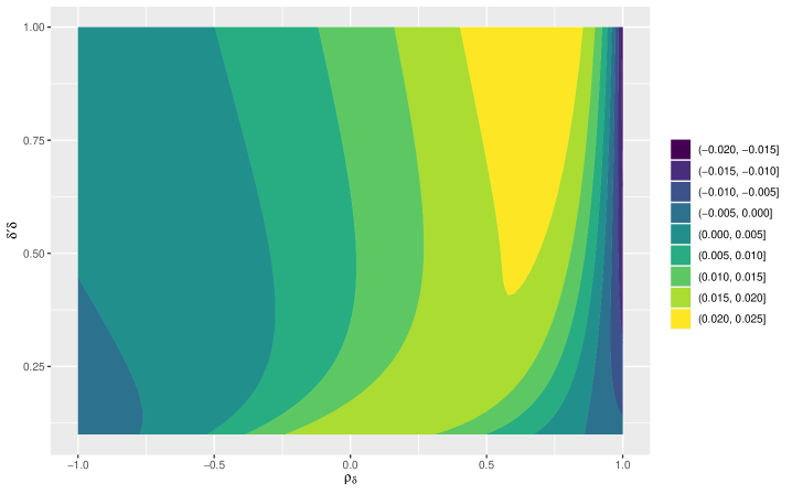
Figure 1: Contour plot of the difference between the violation of the nesting equality with a distilled sample and the violation of the nesting equality with a coarsened propensity score. A positive value implies that the violation with a distilled sample is larger than the violation with a coarsened propensity score. A negative value implies that the violation with a coarsened propensity score is larger that the violation with a distilled sample.

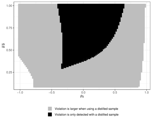
Figure 2: The region of parameter values where the violation of the nesting equality with a distilled sample exceeds the violation of the nesting equality with a coarsened propensity score, and the region where only the nesting equality with a distilled sample is violated. Each point corresponds to a combination of $\rho_{\delta}$ and $\delta^{\prime}\delta$. Let $\mathcal{N}(\rho_{\delta},\delta^{\prime}\delta)$ denote the violation of the nesting equality with a coarsened propensity score defined in (27), and let $\mathcal{D}(\rho_{\delta},\delta^{\prime}\delta)$ denote the violation of the nesting inequality with a distilled sample defined in (28). A point is shaded gray if $\mathcal{D}(\rho_{\delta},\delta^{\prime}\delta)\geq\mathcal{N}(\rho_{\delta},\delta^{\prime}\delta)\geq 0$. A point is shaded black if $\mathcal{D}(\rho_{\delta},\delta^{\prime}\delta)>0$ and $\mathcal{N}(\rho_{\delta},\delta^{\prime}\delta)<0$.

2.6 A Distillation Procedure

As in Proposition 5, consider data such that $p\in P^{-}\cup P^{+}$. Let $i$ index observations. Sort observations $i=1,...,N$ into ascending order by propensity score, so that observation $i=1$ has the lowest propensity score and observation $i=N$ the highest. Split ties by ordering observations with $Z=0$ before observations with $Z=1$. Let $S_{1,i}$ be the sample inclusion indicator for observation $i$. First-order stochastic dominance holds when

$$\frac{\sum_{i=1}^{j}S_{1,i}Z_{i}}{\sum_{i=1}^{n}S_{1,i}Z_{i}}\leq\frac{\sum_{i=1}^{j}S_{1,i}(1-Z_{i})}{\sum_{i=1}^{n}S_{1,i}(1-Z_{i})}\quad\text{for}\>j=1,...,N.$$ (29)

These constraints restrict the conditional propensity score CDF for $Z=1$ to never exceed the conditional CDF for $Z=0$.

It is immediate from (29) that

1. $S_{1,i}=0$ for all $i$ with $Z_{i}=1$ and $p(X_{i},Z_{i})<\underset{j}{\text{min}}(p(X_{j},Z_{j}):Z_{j}=0)$,

2. $S_{1,i}=0$ for all $i$ with $Z_{i}=0$ and $p(X_{i},Z_{i})>\underset{j}{\text{max}}(p(X_{j},Z_{j}):Z_{j}=1)$.

That is, the observation in the trimmed sample with the lowest propensity score must have $Z=0$ and the observation with the highest propensity score must have $Z=1$. In all the applications considered in Section 5, no further trimming is necessary. Assume that we begin with a sample that has been trimmed in this manner, so that $Z_{i}=0$ for $i=1$ and $Z_{i}=1$ for $i=N$. Let $n_{0}$ be the number of observations with $Z=0$ and $n_{1}$ be the number with $Z=1$. Define $\Delta_{j}$ to be the difference between the conditional propensity score distributions for $Z=1$ and $Z=0$ at point $j$

$$\Delta_{j}\equiv\frac{\sum_{i=1}^{j}Z_{i}}{n_{1}}-\frac{\sum_{i=1}^{j}(1-Z_{i})}{n_{0}}.$$

The algorithm is as follows

1. Set $S_{1i}=1\;\forall\;i$

2. Calculate $\Delta_{j}$ for $j=1,...,N$. If $\text{max}(\Delta_{j})\leq 0$, stop. If $\text{max}(\Delta_{j})>0$, continue to steps 3 and 4.

3. Let $J^{-}=\{j:p_{j}\in P^{-}\}$

   1. Find

      $$j^{-} =\underset{j\in J^{-}}{\text{argmax}}\;d_{1j},$$

      $$d_{1} =\underset{j\in J^{-}}{\text{max}}\;d_{1j},$$

      where

      $$d_{1j}=\text{ceil}\left(\frac{n_{0}}{n_{0}-\sum_{i=1}^{j}(1-Z_{i})}n_{1}\Delta_{j}\right),$$

   2. Loop over $j=1,...,j^{-}$. If $Z_{j}=1$

      1. Calculate

         $$\delta_{1j}=\frac{\sum_{i=1}^{j}S_{1,i}Z_{i}}{n_{1}-d_{1}}-\frac{\sum_{i=1}^{j}(1-Z_{i})}{n_{0}}.$$

      2. If $\delta_{1j}>0$, set $S_{1j}=0$

4. Let $J^{+}=\{j:p_{j}\in P^{+}\}$

   1. Find

      $$j^{+} =\underset{j\in J^{+}}{\text{argmax}}\;d_{0j},$$

      $$d_{0} =\underset{j\in J^{+}}{\text{max}}\;d_{0j},$$

      where

      $$d_{0j}=\text{ceil}\left(n_{0}\frac{n_{1}-d_{1}}{\sum_{i=1}^{j}Z_{i}-d_{1}}\left(\Delta_{j}-\frac{d_{1}}{n_{1}-d_{1}}\frac{n_{1}-\sum_{i=1}^{j}Z_{i}}{n_{1}}\right)\right).$$

   2. Loop over $j=N,...,j^{+}+1$. If $Z_{j}=0$

      1. Calculate

         $$\delta_{0j}=\frac{\sum_{i=j}^{N}S_{1,i}(1-Z_{i})}{n_{0}-d_{0}}-\frac{\sum_{i=j}^{N}Z_{i}}{n_{1}-d_{1}}.$$

      2. If $\delta_{0j}>0$, set $S_{1j}=0$

The algorithm begins by including all possible observations. In step 2, it checks if first-order stochastic dominance holds with all possible observations included. If stochastic dominance would not hold, we proceed to steps 3 and 4. Step 3 considers observations with $p\in P^{-}$. In step 3a, the algorithm calculates for each index $j$ the number of observations with $i\leq j$ and $Z_{i}=1$ that need to be trimmed for there to be no violation of stochastic dominance at $p(X_{j},Z_{j})$. Taking the maximum gives the overall number of observations that must be trimmed, $d_{1}$, and the index by which this trimming must take place, $j^{-}$. Step 3b then selects the observations to be trimmed. Looping over $j$ from 1 to $j^{-}$, an observation is trimmed whenever its inclusion would lead the trimmed propensity score distribution for $Z=1$ to cross the propensity score distribution for $Z=0$. Step 4 is analogous to step 3, but instead considers observations with $p\in P^{+}$. Step 4a calculates the number of observations with $i\geq j$ and $Z_{i}=1$ that need to be trimmed for there to be no violation of stochastic dominance at $p(X_{j},Z_{j})$. Taking the maximum of this gives a number of observations to trim, $d_{0}$, and an index above which this trimming must take place $j^{+}$. In step 4b, an observation is trimmed whenever its inclusion would lead the trimmed complementary propensity score distribution for $Z=0$ to cross the trimmed complementary distribution for $Z=0$.

Figure 3 presents an example with artifical data. Panel 3(a) plots the empirical distributions of the propensity scores conditional on $Z$. First-order stochastic dominance is violated as the distribution for $Z=1$ lies above the distribution for $Z=0$ for some $p$. Panel 3(b) plots $d_{1j}$ for each $j\in J^{-}$. In step 3a, $d_{1}$ and $j^{-}$ are found by taking the maximum. In this case, $d_{1}=6$. Panel 3(c) shows step 3b. An observation is trimmed whenever the trimmed propensity score distribution for $Z=1$ would rise above the distribution for $Z=0$. Panel 3(d) plots $d_{0j}$ for each $j\in J^{+}$. In step 4a, $d_{0}$ and $j^{+}$ are found by taking the maximum. In this case $d_{0}=11$. Panel 3(e) shows step 4b. Here an observation is trimmed whenever the trimmed complementary propensity score distribution for $Z=0$ would rise above the trimmed complementary distribution for $Z=1$. Panel 3(f) shows the resulting trimmed distributions, where first-order stochastic dominance holds as required by distillation.

(a) Empirical distributions

(b) Step 3a

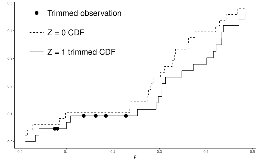
(c) Step 3b

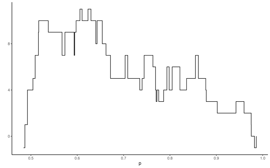
(d) Step 4a

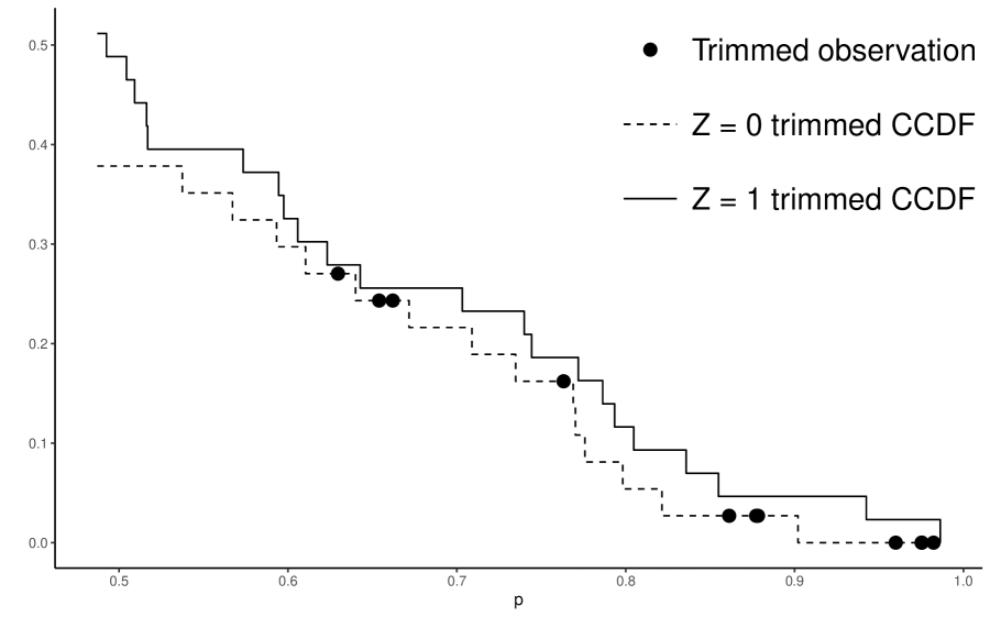
(e) Step 4b

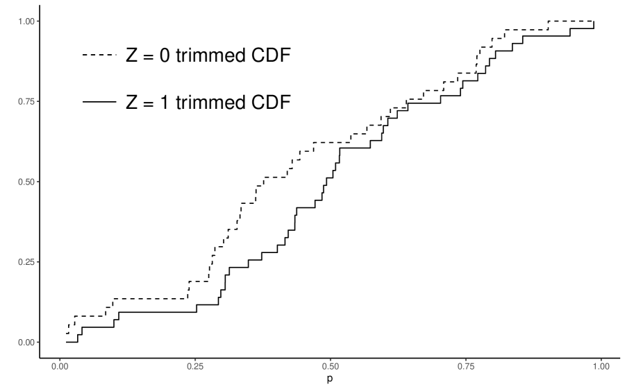
(f) Trimmed distributions

Figure 3: Example of the distillation algorithm. The sample consists of 100 observations. The data generating process sets $\Pr(Z=1)=1/2$ with propensity score uniformly distributed between 0 and 1 for $Z=0,1$. The interval $P^{-}$ includes all observations with a propensity weakly less than the median, while $P^{+}$ includes all observations with a propensity score above the median. Panel 3(b) plots $d_{1j}$ for all $j\in J^{-}$. Panel 3(d) plots $d_{0j}$ for all $j\in J^{+}$.

This algorithm satisfies Definition 3 as first order stochastic dominance is guaranteed to hold for the trimmed sample, and trimming is performed based on propensity score values only. In addition, as all observations with $Z_{i}=0$ and $p\in P^{-}$ or $Z_{i}=1$ and $p\in P^{+}$ are retained

$$\Pr(P\leq p|Z=0,S_{1}=1,p\in P^{-})=\Pr(P\leq p|Z=0,p\in P^{-})$$

$$\Pr(P\leq p|Z=0,p\in P^{+})=\Pr(P\leq p|Z=0,S_{1}=1,p\in P^{+})$$

which is sufficient to satisfy condition (ii) of Proposition 5.

In general there will be many trimmed samples that satisfy Definition 3 and condition (ii) of Proposition 5. To select a particular sample, in this algorithm we choose the observations that are trimmed in order to make the propensity score distributions for $Z=0$ and $Z=1$ as similar as possible. This can be motivated heuristically as follows: variation in subdensities driven by propensity score can mask variation in the subdensities driven by $Z$. Hence, we wish to compare subdensities for similar propensity score distribution.

As the second step of the algorithm does not take into account any subsequent trimming of observations with $Z_{i}=0$, it may trim more observations with $Z_{i}=1$ than is necessary to attain stochastic dominance. Appendix D details how the algorithm may be modified to avoid unnecessary trimming. The additional step essentially determines $d_{0}$ and $d_{1}$ by iterating using the algorithm above, so satisfies the conditions of Definition 3 and condition (ii) of Proposition 5 in the same manner.

3 Test Statistics and Procedure

We set the null hypothesis for our test to be the joint restrictions of index sufficiency (10) and the nesting inequalities with a distilled sample (19) shown in Proposition 4. This section presents the construction of our test statistics and an implementation procedure with a bootstrap algorithm for computing p-values. Our exposition of the test here is restricted to a binary instrument $Z\in\{1,0\}$, while the support of covariates $\mathcal{X}$ is unconstrained. Appendix E presents a test procedure for a single multi-valued discrete instrument.

3.1 Test statistics and bootstrap algorithm

Let $\lambda=\Pr(Z=1)\in(0,1)$ and $(Z,S_{1})\in\{0,1\}\times\{0,1\}$ be a binary instrument and a sample inclusion indicator as defined in Definition 3. With binary $Z$, we can rewrite the nesting inequalities with a distilled sample (19) and index sufficiency of Proposition 2 as the following moment inequalities and equalities: for every measurable subset $A\subset\mathcal{Y}$,

$$E[1\{U_{i}\in A\}D_{i}|Z=0,S_{1}=1]-E[1\{U_{i}\in A\}D_{i}|Z=1,S_{1}=1]\leq 0,$$ (30)

$$E[1\{U_{i}\in A\}(1-D_{i})|Z=1,S_{1}=1]-E[1\{U_{i}\in A\}(1-D_{i})|Z=0,S_{1}=1]\leq 0,$$ (31)

$$E\left[\frac{1\{U_{i}\in A\}D_{i}(1-\lambda)}{\Pr(Z=0|p(X_{i},Z_{i}))}|Z=0,S_{2}=1\right]-E\left[\frac{1\{U_{i}\in A\}D_{i}\lambda}{\Pr(Z=1|p(X_{i},Z_{i}))}|Z=1,S_{2}=1\right]=0,$$ (32)

$$E\left[\frac{1\{U_{i}\in A\}(1-D_{i})(1-\lambda)}{\Pr(Z=0|p(X_{i},Z_{i}))}|Z=0,S_{2}=1\right]-E\left[\frac{1\{U_{i}\in A\}(1-D_{i})\lambda}{\Pr(Z=1|p(X_{i},Z_{i}))}|Z=1,S_{2}=1\right]=0,$$ (33)

where $S_{2}$ is a sample inclusion indicator based on the value of the inverse probability weighting term $\Pr(Z=1|p(X_{i},Z_{i}))$. For example, $S_{2}=1$ if $\Pr(Z=1|p(X_{i},Z_{i}))\in[0.05,0.95]$ and $S_{2}=0$ otherwise. Trimming in this manner avoids dividing by near zero probabilities which regularizes the statistical behaviour of the sample analogues of these expectations.

The inequalities (30) and (31) express the nesting inequalities of Proposition 4 in terms of the conditional expectations given $(Z,S_{1}=1)$. Using Bayes rule, the moment equality hypotheses (32) and (33) express the index sufficiency restrictions of Proposition 2 in terms of the conditional expectation given $(Z,S_{2}=1)$. Trimming the sample through $S_{2}$ does not affect validity of the index sufficiency restrictions insofar as $S_{2}=1$ depends only on the value of the propensity score.

Denote the conditional distributions of $(U,D,X)$ given $Z=1$ and $Z=0$ by $P$ and $Q$, respectively, and the corresponding empirical distributions by $P_{n_{1}}$ and $Q_{n_{0}}$, where $n_{1}$ and $n_{0}$ are the number of observations with $Z=1$ and $Z=0$, respectively. Following the notational conventions of empirical process theory (e.g., Van Der Vaart and Wellner (1996)), we denote the expectation of a function of $(U,D,X,S_{1})$, $f$, with respect to a generic distribution, $P$, by $Pf$ and the sample analogue (sample average) by $P_{n_{1}}f$. Similarly, for a function $g$ of $(U,D,X,S_{2})$, the expectation with respect to a generic distribution $P$ and its sample analogue are denoted by $Pg$ and $P_{n_{1}}g$, respectively.

Let $\mathcal{C}(\mathcal{Y})$ be the class of closed and connected intervals in $\mathcal{Y}$. Define

$$f_{i}^{z}(A,d) =\frac{1\{U_{i}\in A,D_{i}=d\}S_{1i}}{\Pr(S_{1}=1|Z=z)},$$

$$g_{i}^{z}(A,d) =\frac{1\{U_{i}\in A,D_{i}=d\}\lambda^{z}(1-\lambda)^{1-z}S_{2i}}{\Pr(Z=z|p(X_{i},Z_{i}))\Pr(S_{2}=1|Z=z)}.$$

Consider the following test statistic,

$$T\equiv \max\left\{\sup_{A\in\mathcal{C}(\mathcal{Y}),d\in\{0,1\}}\frac{T_{1}(A,d)}{\hat{\sigma}_{1}(A,d)\vee\xi},\sup_{A\in\mathcal{C}(\mathcal{Y}),d\in\{0,1\}}\frac{T_{2}(A,d)}{\hat{\sigma}_{2}(A,d)\vee\xi},\sup_{A\in\mathcal{C}(\mathcal{Y}),d\in\{0,1\}}\frac{-T_{2}(A,d)}{\hat{\sigma}_{2}(A,d)\vee\xi}\right\},\ \text{where}$$

$$T_{1}(A,d)= \sqrt{\frac{n_{1}n_{0}}{n_{1}+n_{0}}}\left[\left(Q_{n_{0}}f_{i}^{0}(A,1)-P_{n_{1}}f_{i}^{1}(A,1)\right)d+(P_{n_{1}}f_{i}^{1}(A,0)-Q_{n_{0}}f_{i}^{0}(A,0))(1-d)\right]$$

$$T_{2}(A,d)= \sqrt{\frac{n_{1}n_{0}}{n_{1}+n_{0}}}\left(Q_{n_{0}}g_{i}^{0}(A,d)-P_{n_{1}}g_{i}^{1}(A,d)\right)$$

$$\hat{\sigma}_{1}^{2}(A,d)= \left\{\lambda[Q_{n_{0}}(f_{i}^{0}(A,1))^{2}-(Q_{n_{0}}f_{i}^{0}(A,1))^{2}]+(1-\lambda)[P_{n_{1}}(f_{i}^{1}(A,1))^{2}-(P_{n_{1}}f_{i}^{1}(A,1))^{2}]\right\}d$$

$$+\left\{\lambda[Q_{n_{0}}(f_{i}^{0}(A,0))^{2}-(Q_{n_{0}}f_{i}^{0}(A,0))^{2}]+(1-\lambda)[P_{n_{1}}(f_{i}^{1}(A,0))^{2}-(P_{n_{1}}f_{i}^{1}(A,0))^{2}]\right\}(1-d),$$

$$\hat{\sigma}_{2}^{2}(A,d)= \lambda[Q_{n_{0}}(g_{i}^{0}(A,d))^{2}-(Q_{n_{0}}g_{i}^{0}(A,d))^{2}]+(1-\lambda)[P_{n_{1}}(g_{i}^{1}(A,d))^{2}-(P_{n_{1}}g_{i}^{1}(A,d))^{2}].$$

Statistic $T$ is a variance-weighted Kolmogorov-Smirnov test statistic that jointly tests (30) - (33) by searching for a maximal violation of their variance-weighted sample analogues. Here, the denominators of the terms appearing in the max operator are consistent estimators for the asymptotic standard deviations of the numerators. $\xi$ is a user-specified trimming constant which serves to bound the denominator away from zero. Similar to the test of Kitagawa (2015), searching over the closed and connected intervals $\mathcal{C}(\mathcal{Y})$ suffices for detecting violations in any measurable set in $\mathcal{Y}$.

Keeping the standard deviation estimators fixed, we want to resample $T_{1}(\cdot,\cdot)$ and $T_{2}(\cdot,\cdot)$ from a distribution such that the null hypothesis holds and their variance-covariance structure is preserved. Specifically, we consider a multiplier bootstrap: let $(\hat{M}_{1},\dots,\hat{M}_{n})$ be iid random bootstrap multipliers such that they are independent of the original sample and satisfy $E(\hat{M}_{i})=0$ and $Var(\hat{M}_{i})=1$. A bootstrap analogue of $T$ under a least favorable null can be constructed as

$$\hat{T}\equiv \max\left\{\sup_{A\in\mathcal{C}(\mathcal{Y}),d\in\{0,1\}}\frac{\hat{T}_{1}(A,d)}{\hat{\sigma}_{1}(A,d)\vee\xi},\sup_{A\in\mathcal{C}(\mathcal{Y}),d\in\{0,1\}}\frac{\hat{T}_{2}(A,d)}{\hat{\sigma}_{2}(A,d)\vee\xi},\sup_{A\in\mathcal{C}(\mathcal{Y}),d\in\{0,1\}}\frac{-\hat{T}_{2}(A,d)}{\hat{\sigma}_{2}(A,d)\vee\xi}\right\},\ \text{where}$$

$$\hat{T}_{1}(A,d)= \sqrt{\frac{n_{1}n_{0}}{n_{1}+n_{0}}}\left((\hat{Q}_{n_{0}}-Q_{n_{0}})f_{i}^{0}(A,1)-(\hat{P}_{n_{1}}-P_{n_{1}})f_{i}^{1}(A,1)\right)d$$

$$+\sqrt{\frac{n_{1}n_{0}}{n_{1}+n_{0}}}\left((\hat{P}_{n_{1}}-P_{n_{1}})f_{i}^{1}(A,0)-(\hat{Q}_{n_{0}}-Q_{n_{0}})f_{i}^{0}(A,0)\right)(1-d)$$

$$\hat{T}_{2}(A,d)= \sqrt{\frac{n_{1}n_{0}}{n_{1}+n_{0}}}\left[(\hat{Q}_{n_{0}}-Q_{n_{0}})g_{i}^{0}(A,d)-(\hat{P}_{n_{1}}-P_{n_{1}})g_{i}^{1}(A,d)\right],$$

where, for the random variable $(a_{i}:i=1,\dots,n)$, we define

$$(\hat{Q}_{n_{0}}-Q_{n_{0}})a_{i} =\frac{1}{n_{0}}\sum_{i:Z_{i}=0}\hat{M}_{i}a_{i},\mspace{10.0mu}(\hat{P}_{n_{1}}-P_{n_{1}})a_{i}=\frac{1}{n_{1}}\sum_{i:Z_{i}=1}\hat{M}_{i}a_{i}.$$

3.1.1 Test Procedure

An implementation of the test is as follows.

1. Estimate the propensity scores $\Pr(D=1|Z,X)$ using either parametric or nonparametric methods, and obtain the fitted values $\hat{p}\left(x_{i},z_{i}\right)$.

2. Estimate the partially linear regression model (6) and obtain estimates of $\theta_{1}$ and $\theta_{0}$.  Specifically, let $\hat{\mu}_{x,i}=\hat{E}\left(x_{i}|\hat{p}\left(x_{i},z_{i}\right)\right)$ be nonparametric regression estimates (e.g. local linear predicted values) of the covariate vector $x_{i}$ onto the estimated propensity scores, $\hat{p}_{i}\equiv\hat{p}\left(x_{i},z_{i}\right),$ and let $\hat{\mu}_{y,i}=\hat{E}\left(y_{i}|\hat{p}\left(x_{i},z_{i}\right)\right)$ be a nonparametric regression estimate of the outcome onto the estimated propensity scores.  $\left(\theta_{0},\theta_{1}\right)$ can be estimated by running OLS on

   $$y_{i}-\hat{\mu}_{y,i}=\hat{p}_{i}\left(x_{i}-\hat{\mu}_{x,i}\right)\theta_{1}+\left(1-\hat{p}_{i}\right)\left(x_{i}-\hat{\mu}_{x,i}\right)\theta_{0}+\epsilon_{i}.$$

3. Construct the residual observations by $\hat{u}_{i}=D_{i}\left(y_{i}-x_{i}^{\prime}\hat{\theta}_{1}\right)+(1-D_{i})\left(y_{i}-x_{i}^{\prime}\hat{\theta}_{0}\right)$.

4. Construct the inclusion indicators $S_{1}$. This can be done using the algorithm of Section 2.5.

5. Estimate $\Pr(Z=1|p(X,Z))$ and generate the inclusion indicators $S_{2}$

6. Using $\left(\hat{u}_{i},D_{i},z,\hat{\Pr}(Z=1|p(X,Z),S_{1,i},S_{2,i}\right)$ as data, calculate the test statistic of Section 3.1

The test procedure described above involves semiparametric estimation of a partially linear model where each conditioning covariate and the outcome are non-parametrically regressed on the propensity score. While non-parametric estimation can be computationally taxing, this step is only performed once and the main determinant of the computational burden is the sample size rather than the number of conditioning covariates. In cases where this non-parametric estimation step is infeasible, the test procedure can still be implemented by specifying a parametric functional form for $\phi(p)$, such as a quadratic polynomial in the propensity score.

3.2 Practical Considerations

3.2.1 Testing Causal Intepretability of 2SLS

The test proposed here does not directly test instrument validity in the context of linear 2SLS. This is because the set of identifying assumptions considered in Proposition 2 is distinct from the set of conditions that allows us to interpret the linear two-stage least square (2SLS) estimand as a weighted average of LATEs/MTEs with positive weights. Specifically, causal interpretability of linear 2SLS requires only the weaker exogeneity condition (A2), not the strong exogeneity of (A5), and does not require the functional form specification for the potential outcome equations of (A4). On the other hand, as shown in Abadie (2003), Kolesár (2013), Słoczyński (2021), and Blandhol et al. (2022), causal interpretability of 2SLS relies crucially on the linearity of $E(Z|X)$ in the covariate vector $X$, whereas the identifying assumptions here considered place no restrictions on $E(Z|X)$.

However, we believe our test is useful as a specification check when one reports linear 2SLS estimates for the following reasons. First, non-rejection in our test means the data do not reject strong exogeneity (A5), implying that the data also do not contradict weak exogeneity (A2). With credible evidence for the linearity of $E(Z|X)$, non-rejection of our test can be used to support causal interpretability of linear 2SLS. Second, with specifications of the potential outcome equations and the propensity score, our test is useful for checking which variables should be included as controlling covariates. Hence, p-values of our test can also suggest which set of covariates should be included in the linear 2SLS estimation.

3.2.2 Continuous Instruments

The test procedure can accommodate continuous instruments as follows. The initial estimation of a partially linear model can be performed using the continuous instrument. With estimated partial residuals in hand, the instrument can then be discretized, and the test procedure for a multi-valued discrete instrument of Appendix E applied.

3.2.3 Multiple Instruments

The discussion to this point has considered only a scalar $Z$, here we consider the case where $Z$ is a vector of multiple instruments. Propositions 1 and 2 hold irrespective of the number of instruments. Hence, both testable implications remain available. However, a test of the nesting inequalities using a coarsened propensity score would be subject to the same concerns regarding power as the single instrument case.

Consider the case of two binary instruments $Z=(Z_{1},Z_{2})$, $Z_{1}\in\{0,1\}$, $Z_{2}\in\{0,1\}$. When testing nesting inequalities and index sufficiency, $Z$ can be treated as a single instrument taking four values. That is, the estimation step is performed taking $Z$ to be vector, but when testing we map from $(0,0),(0,1),(1,0),(1,1)$ to four values of a single categorical variable and implement the test for a multi-valued instrument described in Appendix E. In cases where this is not viable, one approach is to aggregate the multiple instruments into a single index, and then treat this index as single multivalued instrument. Suppose the propensity score has a generalised linear form with a probit link

$$p(X,Z)=\Phi(\rho X+\varphi(Z)),$$ (34)

where $\varphi(\cdot)$ reflects the researchers assumptions about the relationship between the instruments and $Z$ and $\rho$ is a vector of coefficients. In this case, we view $\varphi(Z)$ as an aggregated index of instruments, and perform the test as if it was a single instrument.

Our testing approach can be extended to the setting of Mogstad et al. (2019, 2020) where the montonicity assumption Imbens and Angrist (1994) is replaced by partial monotonicity. Mogstad et al. (2019, 2020) show that inference using a single instrument remains valid as long as the remaining instruments are controlled for. In the context of our test procedure, the estimation of the propensity score and residuals would be performed using the entire set of instruments, but the final step would be performed separately for each instrument. That is, index sufficiency and the nesting inequalities are tested for every instrument, with a distilled sample used in the test of nesting inequalities. A Bonferroni correction can be applied to P-values to correct for multiple tests.

4 Monte Carlo

We perform two sets of Monte Carlo exercises. The first evaluates the size and power of the joint test of nesting inequalities with a distilled sample and index sufficiency, and compares it to the Kitagawa (2015) test which does not control for covariates and the test of the nesting inequalities using a coarsened propensity score. The second looks separately at the power of the tests of index sufficiency and nesting inequalities with a distilled sample.

All exercises use

$$X\sim\text{N}_{3}(0_{3},I_{3})$$ (35)

$$Z=\mathbbm{1}\{X^{\prime}\gamma+U_{Z}\geq 0\}$$ (36)

$$D=\mathbbm{1}\{\alpha_{0}(1-Z)+\alpha_{1}Z+X^{\prime}\delta+U_{D}\geq 0\}$$ (37)

$$Y=DY_{1}+(1-D)Y_{0}$$ (38)

$$Y_{0}=X^{\prime}\theta+\tilde{U}_{0}$$ (39)

$$U_{Z}\sim N(0,1)$$ (40)

$$(\tilde{U}_{0},U_{D})\sim N(0,\Sigma),$$ (41)

with diagonal entries of $\Sigma$ set to 1 and off-diagonal entries to 0.3. Elements of $\theta$ are drawn from the uniform distribution with bounds $(-1,1)$. The distributions for $\gamma$ and $\delta$ are described below. $\alpha_{0}$, $\alpha_{1}$, and the specification for $Y_{1}$ differ for the size and power processes. When checking size we consider a valid a but irrelevant instrument

$$\alpha_{0}=\alpha_{1}=0,$$ (42)

$$Y_{1}=X^{\prime}\theta+1+\tilde{U}_{1},\ \text{with $\tilde{U}_{1}=\tilde{U}_{0}$.}$$ (43)

Here, conditional on the propensity score, the joint distribution of $(U,D)$ conditional on $Z$ is identical for $Z=0$ and $Z=1$. Four specifications are used to check power. They share

$$\alpha_{0}=\Phi^{-1}(0.45),$$ (44)

$$\alpha_{1}=\Phi^{-1}(0.55),$$ (45)

$$Y_{1}=X^{\prime}\theta+\tilde{U}_{1},$$ (46)

where $\Phi^{-1}()$ is the standard normal quantile function. The specifications for $\tilde{U}_{1}$ are

DGP1: $$\tilde{U}_{1}=Z\times\tilde{U}_{0}+(1-Z)\times(-0.7+\tilde{U}_{0}),$$

DGP2: $$\tilde{U}_{1}=Z\times\tilde{U}_{0}+(1-Z)\times 1.675\times\tilde{U}_{0},$$

DGP3: $$\tilde{U}_{1}=Z\times\tilde{U}_{0}+(1-Z)\times 0.515\times\tilde{U}_{0},$$

DGP4: $$\tilde{U}_{1}=Z\times\tilde{U}_{0}+(1-Z)\times(\mu_{l}+0.125\times\tilde{U}_{0}),$$

where $\mu_{l}$ takes values $(-1,-0.5,0,0.5,1)$ with probabilities $(0.15,0.2,0.3,0.2,0.15)$. Figure 4 plots the densities of $(\tilde{U}_{1},D=1|Z)$ for each of the four processes for one draw of parameters. In the case of DGP1 the distribution for $Z=0$ is shifted, with DGP2 it has thicker tails, with DGP3 it is more concentrated, and with DGP4 there are violations at each value of $\mu_{l}$. In all cases, for a given propensity score, the distribution of $(\tilde{U}_{1},D=1)$ conditional on $Z$ does not coincide for $Z=0$ and $Z=1$.

We consider three values of the sample size $N$: 200, 500, and 1000. For each process and sample size, we generate 1,000 samples. When comparing test procedures, the same simulated samples are used for each test procedure. The proposed test procedure requires estimating propensity scores, a partially linear model for outcomes, and $\Pr(Z=1|p(X,Z))$. Propensity scores are estimated by probit with the correct specification supplied. For the nonparametric regressions involved in the estimation of the partially linear model we use local linear regressions. For the estimation of $\Pr(Z=1|p(X,Z))$, we use local constant regressions. In both cases bandwidths are chosen by least squares cross validation. The partially linear model is estimated under the assumption that the instrument is valid, so the specification is

$$Y=X^{\prime}\theta+\phi(p)+\epsilon.$$

In the case DGP1-DGP4, this specification is incorrect, so estimates will be biased. We set the sample inclusion indicator for the index sufficiency test to $S_{2}=\mathbbm{1}\{\Pr(Z=1|p(X,Z))\in[0.05,0.95]\}$. Results are reported for two values of the trimming parameter $\xi$: $\sqrt{0.05\times 0.95}\approx 0.21$ and 0.3. Results for additional values of $\xi$ are available upon request. P-values are calculated using 500 bootstrap samples.

4.1 Size and Power

Here we evaluate the size and power of the proposed test procedure, and compare it to the Kitagawa (2015) test that does not control for covariates and the test of nesting inequalities with a binarised propensity score.

For this exercise, the elements of $\delta$ are drawn from the uniform distribution with bounds $(-1,1)$. For $\gamma$, we consider two cases. The first sets all elements of $\gamma$ to 0. $X$ and $Z$ are then independent, so an instrument that is valid conditional on the covariates will also be valid without conditioning on covariates and failure to control appropriately for $X$ should not affect size. In the second case each element of $\gamma$ is drawn from the uniform distribution with bounds $(-1,1)$. Here $X$ and $Z$ will not, in general, be independent, and the instrument can only be valid conditional on $X$.

Tables 1 and 2 present rejection rates. Turning first to the proposed test procedure, rejection rates for the size process are below nominal size irrespective of whether $X$ and $Z$ are independent. For the four power DGPs, with the exception of the smaller sample sizes for DGP4, all rejection rates are well above the nominal size. Similar rejection rates are obtained irrespective of whether $X$ and $Z$ are independent.

Next consider the test with a binarised propensity score. This test performs well in terms of size: rejection rates for the size processes are below nominal size. However, consistent with the results of Proposition 5, there is a considerable loss in power compared to the proposed test procedure. Rejection rates above nominal size are obtained only for DGP1. For all other DGPs, rejection rates are low and change little as the sample size increases.

Figures 5 and 6 illustrate why the test with a binarized propensity score lacks power. To construct these figures, for each of the four power DGPs, we generate a single draw for $\theta$ and $\delta$. To simplify, $\gamma$ is set to the zero vector. We approximate the asymptotic estimates of $\theta$, $\hat{\theta}^{\star}$, by generating a sample of a million observations and regressing $Y-E[Y|p]$ on $X-E[X|p]$. Partial residuals are then calculated as $U=Y-X^{\prime}\hat{\theta}^{\star}$. Figure 5 plots the densities of $(U,D=1)$ conditional on $Z=0$ and $Z=1$, whereas Figure 6 plots the subdensities conditional on the binarised propensity score $Z^{*}$. In Figure 5, when we condition on $Z$, violations of the null are apparent in all cases, but in Figure 6 violations are either small or have vanished entirely. Each value of $Z^{*}$ mixes observations with $Z=0$ and $Z=1$. The subdensities in Figure 6 are thus a mixture of those in Figure 5, which masks differences in shape. Furthermore, by construction, all observations with $Z^{*}=0$ have a lower propensity score than observations with $Z^{*}=1$, so the $D=1$ subdensity for $Z^{*}=0$ is guaranteed to have less total mass than the subdensity for $Z^{*}=1$.

The Kitagawa (2015) test, which does not control for covariates, performs reasonably well when the instrument is independent of the covariates. The size of the test is controlled, but power is lower than the proposed test procedure. This is for two reasons. First, the Kitagawa (2015) test essentially tests the nesting inequalities only, and some violations are more easily detected by index sufficiency. Second, failure to control for covariates adds noise to the outcome and which makes violations of the nesting inequalities more difficult to detect. For a single draw of $\theta$ and $\delta$, and with $\gamma$ set to zero, Figure 7 plots the densities of $(Y,D=1)$ conditional on $Z=0$ and $Z=1$ for each DGP. These differ from the densities of Figure 4 as the effect of the covariates on the outcome has not been partialed out. Compared to the densities in Figure 4, violations are either reduced or have vanished entirely. As expected, when $Z$ and $X$ are not independent, this test procedure has rejection rates above nominal size regardless of whether the instrument is valid conditional on covariates.

	$\gamma_{k}=0$						$\gamma_{k}\sim U(-1,1)$
Trimming Constant:	$\xi\approx 0.21$			$\xi=0.30$			$\xi\approx 0.21$			$\xi=0.30$
Nominal Size:	0.1	0.05	0.01	0.1	0.05	0.01	0.1	0.05	0.01	0.1	0.05	0.01
Proposed test procedure
200	0.027	0.004	0.000	0.018	0.005	0.000	0.085	0.040	0.012	0.048	0.022	0.008
500	0.024	0.005	0.000	0.018	0.004	0.000	0.068	0.033	0.009	0.045	0.022	0.007
1000	0.028	0.009	0.002	0.017	0.006	0.000	0.060	0.029	0.010	0.040	0.016	0.003
Binarised $p(X,Z)$
200	0.043	0.024	0.013	0.031	0.023	0.013	0.046	0.033	0.017	0.044	0.030	0.017
500	0.067	0.052	0.035	0.054	0.043	0.029	0.056	0.042	0.033	0.045	0.039	0.029
1000	0.075	0.069	0.051	0.062	0.053	0.040	0.096	0.082	0.060	0.081	0.068	0.048
Kitagawa (2015)
200	0.131	0.070	0.016	0.134	0.067	0.017	0.454	0.384	0.262	0.453	0.403	0.268
500	0.135	0.066	0.015	0.116	0.063	0.012	0.524	0.483	0.403	0.530	0.485	0.404
1000	0.115	0.066	0.012	0.124	0.054	0.012	0.645	0.599	0.540	0.642	0.608	0.539

Table 1: Size

	$\gamma_{k}=0$						$\gamma_{k}\sim U(-1,1)$
Trimming Constant:	$\xi\approx 0.21$			$\xi=0.30$			$\xi\approx 0.21$			$\xi=0.30$
Nominal Size:	0.1	0.05	0.01	0.1	0.05	0.01	0.1	0.05	0.01	0.1	0.05	0.01
Power DGP1
Proposed test procedure
200	0.164	0.085	0.020	0.158	0.078	0.018	0.228	0.144	0.059	0.189	0.113	0.042
500	0.446	0.311	0.104	0.440	0.309	0.110	0.454	0.328	0.154	0.413	0.289	0.124
1000	0.725	0.587	0.346	0.718	0.586	0.327	0.706	0.569	0.327	0.676	0.548	0.300
Binarised Propensity Score
200	0.053	0.040	0.012	0.050	0.040	0.011	0.049	0.035	0.013	0.044	0.028	0.013
500	0.153	0.128	0.074	0.131	0.104	0.064	0.127	0.096	0.051	0.096	0.079	0.045
1000	0.313	0.263	0.192	0.251	0.214	0.150	0.266	0.232	0.158	0.225	0.183	0.114
Kitagawa (2015)
200	0.205	0.134	0.039	0.198	0.123	0.033	0.419	0.354	0.249	0.417	0.358	0.251
500	0.359	0.257	0.122	0.354	0.255	0.118	0.583	0.535	0.450	0.577	0.530	0.448
1000	0.637	0.545	0.362	0.652	0.548	0.342	0.699	0.668	0.604	0.690	0.656	0.591
Power DGP2
Proposed test procedure
200	0.201	0.116	0.026	0.206	0.118	0.031	0.232	0.146	0.039	0.200	0.124	0.033
500	0.638	0.493	0.194	0.648	0.505	0.195	0.585	0.432	0.167	0.529	0.387	0.145
1000	0.954	0.908	0.697	0.955	0.902	0.684	0.921	0.858	0.640	0.885	0.791	0.532
Binarised Propensity Score
200	0.026	0.018	0.008	0.023	0.019	0.009	0.039	0.029	0.014	0.041	0.026	0.016
500	0.036	0.027	0.017	0.025	0.021	0.012	0.043	0.033	0.020	0.035	0.029	0.018
1000	0.040	0.032	0.018	0.029	0.021	0.012	0.047	0.038	0.025	0.039	0.032	0.015
Kitagawa (2015)
200	0.105	0.054	0.011	0.079	0.033	0.009	0.369	0.313	0.196	0.372	0.303	0.190
500	0.214	0.141	0.054	0.118	0.070	0.027	0.582	0.526	0.404	0.533	0.477	0.381
1000	0.470	0.366	0.215	0.290	0.200	0.082	0.720	0.680	0.592	0.650	0.602	0.518
Power DGP3
Proposed test procedure
200	0.209	0.116	0.024	0.185	0.098	0.020	0.295	0.189	0.059	0.223	0.142	0.047
500	0.777	0.640	0.303	0.649	0.500	0.185	0.772	0.660	0.364	0.669	0.535	0.268
1000	0.991	0.980	0.925	0.976	0.954	0.827	0.987	0.977	0.901	0.967	0.944	0.784
Binarised Propensity Score
200	0.028	0.020	0.008	0.027	0.018	0.007	0.027	0.016	0.007	0.025	0.015	0.007
500	0.018	0.016	0.012	0.018	0.015	0.010	0.025	0.016	0.010	0.019	0.016	0.009
1000	0.006	0.004	0.003	0.005	0.005	0.002	0.013	0.010	0.006	0.012	0.009	0.003
Kitagawa (2015)
200	0.115	0.061	0.013	0.105	0.058	0.014	0.359	0.301	0.200	0.352	0.294	0.204
500	0.118	0.073	0.022	0.126	0.076	0.027	0.497	0.437	0.338	0.508	0.456	0.349
1000	0.163	0.108	0.039	0.180	0.125	0.042	0.582	0.547	0.475	0.582	0.545	0.478
Power DGP4
Proposed test procedure
200	0.052	0.018	0.002	0.031	0.011	0.001	0.130	0.067	0.013	0.078	0.038	0.008
500	0.302	0.177	0.036	0.125	0.056	0.007	0.326	0.212	0.061	0.194	0.110	0.027
1000	0.732	0.616	0.364	0.412	0.278	0.068	0.710	0.609	0.340	0.471	0.312	0.098
Binarised Propensity Score
200	0.022	0.015	0.007	0.017	0.011	0.007	0.023	0.017	0.009	0.021	0.014	0.009
500	0.021	0.018	0.012	0.018	0.015	0.011	0.040	0.028	0.015	0.022	0.019	0.012
1000	0.016	0.012	0.007	0.011	0.009	0.005	0.028	0.021	0.016	0.019	0.015	0.012
Kitagawa (2015)
200	0.081	0.040	0.003	0.066	0.029	0.004	0.346	0.288	0.176	0.358	0.291	0.186
500	0.080	0.035	0.007	0.071	0.042	0.005	0.451	0.399	0.318	0.453	0.406	0.328
1000	0.076	0.044	0.010	0.078	0.046	0.012	0.527	0.485	0.418	0.532	0.494	0.424

Table 2: Power

4.2 Comparison of Index Sufficiency and Nesting Inequalities

Our second exercise compares the nesting inequality and index sufficiency tests. Section 2 argued that the relative power of testing nesting inequalities and index sufficiency will depend on similarity between propensity score distributions conditional on $Z$. To examine this more formally, we compare rejection rates foe the nesting inequalities and index sufficiency in two cases. Both set all elements of $\gamma$ to 0, so that the instrument and covariates are independent. In the first, the elements of $\delta$ are drawn from the uniform distribution with bounds $(-1,1)$, as in section 4.1. In the second, the elements of $\delta$ are drawn from the uniform distribution with bounds $(-0.1,0.1)$. This second case limits the influence of covariates on the propensity score, which in turn limits the overlap of the conditional propensity score distributions for $Z=0$ and $Z=1$. Figure 8 plots the density of propensity scores conditional on $Z=0$ and $Z=1$ for different values of $\delta$. As the elements of $\delta$ grow larger in magnitude, the densities overlap more. Figure 9 plots the $\Pr(Z=1|p(X,Z))$ function associated with each value of $\delta$. For the smallest $\delta$ this function is close to a step function but, as the elements of $\delta$ grow in magnitude, it becomes flatter.

Table 3 presents rejection rates. When the elements of $\delta$ are drawn from the uniform distribution with bounds $(-1,1)$, index sufficiency has higher rejection rates. When the elements of $\delta$ are drawn from the uniform distribution with bounds $(-0.1,0.1)$, index sufficiency loses power in all cases. Nesting inequalities now have considerably higher power for DGP1, slightly higher power for DGP2 and DGP3, while index sufficiency still exhibits more power for DGP4. In all cases, the overall rejection rate is close to the maximum of the rejection rates for the nesting inequalities and index sufficiency. This suggests that testing both testable implications jointly dominates testing only one of them.

	$\delta_{k}\sim U(-1,1)$						$\delta_{k}\sim U(-0.1,0.1)$
Trimming Constant:	$\xi\approx 0.21$			$\xi=0.30$			$\xi\approx 0.21$			$\xi=0.30$
Nominal Size:	0.1	0.05	0.01	0.1	0.05	0.01	0.1	0.05	0.01	0.1	0.05	0.01
Power DGP 1
Nesting:
200	0.075	0.036	0.004	0.067	0.033	0.003	0.092	0.044	0.006	0.081	0.039	0.003
500	0.256	0.160	0.040	0.251	0.157	0.034	0.401	0.275	0.087	0.386	0.261	0.076
1000	0.558	0.434	0.236	0.529	0.409	0.213	0.859	0.762	0.495	0.840	0.756	0.449
Index Sufficiency:
200	0.174	0.090	0.023	0.173	0.088	0.022	0.103	0.050	0.013	0.085	0.043	0.008
500	0.460	0.318	0.111	0.445	0.310	0.115	0.196	0.104	0.015	0.167	0.086	0.016
1000	0.708	0.574	0.349	0.710	0.573	0.328	0.316	0.216	0.086	0.330	0.214	0.074
Overall:
200	0.164	0.085	0.020	0.158	0.078	0.018	0.101	0.057	0.007	0.084	0.046	0.003
500	0.446	0.311	0.104	0.440	0.309	0.110	0.363	0.211	0.066	0.321	0.205	0.056
1000	0.725	0.587	0.346	0.718	0.586	0.327	0.808	0.718	0.453	0.786	0.692	0.403
Power DGP 2
Nesting:
200	0.048	0.019	0.000	0.025	0.007	0.000	0.063	0.024	0.000	0.027	0.006	0.000
500	0.315	0.186	0.053	0.137	0.074	0.013	0.380	0.227	0.059	0.176	0.085	0.019
1000	0.816	0.675	0.375	0.474	0.305	0.082	0.886	0.791	0.505	0.619	0.442	0.180
Index Sufficiency:
200	0.224	0.126	0.033	0.227	0.130	0.035	0.148	0.075	0.011	0.158	0.074	0.010
500	0.656	0.510	0.214	0.661	0.519	0.209	0.406	0.266	0.095	0.402	0.272	0.097
1000	0.951	0.911	0.705	0.961	0.912	0.702	0.769	0.673	0.403	0.748	0.634	0.372
Overall:
200	0.201	0.116	0.026	0.206	0.118	0.031	0.126	0.049	0.006	0.114	0.055	0.005
500	0.638	0.493	0.194	0.648	0.505	0.195	0.426	0.288	0.093	0.353	0.223	0.071
1000	0.954	0.908	0.697	0.955	0.902	0.684	0.898	0.805	0.527	0.759	0.612	0.337
Power DGP 3
Nesting:
200	0.122	0.063	0.010	0.143	0.074	0.010	0.116	0.056	0.012	0.124	0.063	0.010
500	0.385	0.247	0.077	0.435	0.278	0.083	0.382	0.275	0.097	0.425	0.302	0.108
1000	0.816	0.710	0.451	0.846	0.753	0.475	0.765	0.657	0.363	0.818	0.691	0.398
Index Sufficiency:
200	0.232	0.132	0.027	0.199	0.110	0.022	0.157	0.070	0.014	0.136	0.069	0.015
500	0.792	0.659	0.326	0.672	0.522	0.199	0.462	0.363	0.158	0.414	0.296	0.110
1000	0.991	0.981	0.928	0.977	0.958	0.836	0.667	0.613	0.452	0.667	0.585	0.382
Overall:
200	0.209	0.116	0.024	0.185	0.098	0.020	0.131	0.061	0.008	0.114	0.055	0.009
500	0.777	0.640	0.303	0.649	0.500	0.185	0.475	0.367	0.147	0.434	0.320	0.111
1000	0.991	0.980	0.925	0.976	0.954	0.827	0.832	0.740	0.488	0.829	0.731	0.443
Power DGP 4
Nesting:
200	0.028	0.008	0.001	0.022	0.007	0.001	0.039	0.017	0.002	0.027	0.012	0.002
500	0.064	0.034	0.005	0.050	0.029	0.004	0.094	0.038	0.005	0.063	0.031	0.002
1000	0.170	0.102	0.030	0.142	0.077	0.020	0.231	0.122	0.031	0.161	0.078	0.013
Index Sufficiency:
200	0.064	0.021	0.003	0.040	0.015	0.002	0.054	0.026	0.001	0.050	0.024	0.002
500	0.321	0.186	0.041	0.141	0.061	0.009	0.174	0.113	0.032	0.106	0.048	0.013
1000	0.748	0.630	0.376	0.431	0.292	0.082	0.458	0.372	0.196	0.284	0.188	0.065
Overall:
200	0.052	0.018	0.002	0.031	0.011	0.001	0.055	0.020	0.002	0.034	0.018	0.001
500	0.302	0.177	0.036	0.125	0.056	0.007	0.161	0.088	0.023	0.082	0.035	0.006
1000	0.732	0.616	0.364	0.412	0.278	0.068	0.451	0.342	0.154	0.250	0.149	0.042

Table 3: Comparison of index sufficiency and nesting inequalities

Figure 4: Conditional subdensities of $(\tilde{U}_{1},D=1)$ for DGPs 1 - 4 given values of $\theta$ and $\delta$ drawn from the $U(-1,1)$ distribution. The elements of $\gamma$ are set to 0.

Figure 5: Subdensities of $(U,D=1)$ for DGPs 1 - 4 conditional on the instrument $Z$, where $U=Y-X^{\prime}\beta^{*}$ with $\beta^{*}=\text{plim}\;\hat{\beta}$s of $\theta$ and $\delta$. The elements of $\beta$ are drawn from the $U(0.5,1)$ distribution with random flips of their signs and the elements of $\delta$ are drawn from the $U(-1,1)$ distribution. All elements of $\gamma$ are set to 0.

Figure 6: Subdensities of $(U,D=1)$ for DGPs 1 - 4 conditional on the binarised propensity score, where $U=Y-X^{\prime}\theta^{*}$ with $\theta^{*}=\text{plim}\;\hat{\theta}$, and given the values of $\theta$ and $\delta$. The elements of $\theta$ are drawn from the $U(0.5,1)$ distribution with random flips of their signs and the elements of $\delta$ are drawn from the $U(-1,1)$ distribution. All elements of $\gamma$ are set to 0.

Figure 7: Subdensities of $(Y,D=1)$ for DGPs 1 - 4 conditional on the instrument $Z$ given $\beta$ and $\delta$.he elements of $\beta$ are drawn from the $U(0.5,1)$ distribution with random flips of their signs and the elements of $\delta$ are drawn from the $U(-1,1)$ distribution.

Figure 8: Density of $p(X,Z)$ conditional on $Z=0$ and $Z=1$ for four values of $\delta$ with $\gamma$ set to 0.

Figure 9: $Pr(Z=1|p(X,Z))$ for four values of $\delta$ with $\gamma$ set to 0.

5 Applications

In this section we apply the proposed test procedure to the instrumental variables of Card (1993), Angrist and Evans (1998), and Oreopoulos (2006). In all cases we maintain the outcome, treatment, instrument and conditioning covariates of the original design, and estimate a potential outcome model of the form described in Section 2. For the propensity score, we estimate a probit with the instrument, conditioning covariates and interactions between the two as controls. For the outcome, we allow coefficients on the covariates to depend on the treatment. In the case of Card (1993) and Angrist and Evans (1998), the partially linear model is estimated as described in step 2 of Section 3.1.1, with local linear regressions used to estimate $E[X|p]$ and $E[Y|p]$. $\Pr(Z=1|p)$ is estimated by local constant regressions. Bandwidths are selected by least squares cross validation. For Oreopoulos (2006), the partially linear model is estimated by assuming that the nonparametric component $\phi(p)$ is a cubic polynomial in $p$, and $\Pr(Z=1|p)$ is estimated by probit.

Table 5 presents p-values. A p-value below 0.05 corresponds to a rejection of the null hypothesis at the 5% level of significance. p-values are reported for a range of values of the trimming parameter $\xi$. For each application, Table 5 shows the number of observations in the data set, and the number of observations included in the trimmed samples used in the tests of nesting inequalities with a distilled sample and index sufficiency.

	$\xi\approx 0.07$	$\xi\approx 0.21$	$\xi=0.30$	$\xi=1$
Card (1993)
Nesting inequalities	0.360	0.996	0.998	0.998
Index sufficiency	0.190	0.328	0.248	0.180
Overall	0.210	0.354	0.268	0.198
Angrist and Evans (1998)
Nesting inequalities	0.636	0.986	0.996	0.998
Index sufficiency	0.908	0.766	0.666	0.490
Overall	0.876	0.842	0.734	0.490
Oreopoulos (2006)
Nesting inequalities	0.000	0.000	0.000	0.006

Table 4: P-values for the test of nesting inequalities, the test of index sufficiency, and the combined test of both. A P-value below 0.05 indicates that the null hypothesis would be rejected at the 5% level of significance. $\xi$ is a user specified trimming parameter as described in Kitagawa (2015). For Card (1993) conditioning covariates are residence in the South, residence in a standard metropolitan statistical area in 1966, residence in a standard metropolitan statistical area in 1976, race, a quadratic in potential experience, living in a single mother household at age 14, living with both parents at age 14, mother’s and father’s years of education, dummies for mother’s and father’s years of education being missing, a nine value categorical variable constructed by interacting father’s and mother’s education class, and a categorical variable for region of residence in 1966. Covariates for Angrist and Evans (1998) are mother’s current age, mother’s age at the time of the birth of their first child, the sex of the first child, and two dummies for race. Conditioning covariates for Oreopoulos (2006) are a quartic in age, survey year fixed effects, year aged 14 fixed effects, sex and a dummy for residence in Northern Ireland.

	Observations	Nesting inequalities	Index sufficiency
Card (1993)	3010	3010	3010
Angrist and Evans (1998)	12732	12731	752
Oreopoulos (2006)	82908	82908	0

Table 5: The number of observations in the original sample, the number of observations used in the test of nesting inequalities, and the number of observations used in the test of index sufficiency. Observations are removed for the test of nesting inequalities in order to attain stochastic dominance in the trimmed sample. Observations are removed for the test of index sufficiency if $\Pr(Z=1|p(X,Z))\leq 0.05$ or $\Pr(Z=1|p(X,Z))\geq 0.95$

5.1 Card (1993)

Card (1993) estimates returns to education. The outcome $Y$ is the logarithm of weekly earnings, $D$ is years of education, and $Z$ is growing up in a local labour market with an accredited four year college. The headline specification uses four ordered discrete, three categorical and six binary conditioning covariates. These include potential experience, parental education, and residence in a standard metropolitan statistical area (SMSA). The sample consists of 3,010 observations.

The validity of this instrument has previously been tested by Huber and Mellace (2015), Kitagawa (2015), Mourifié and Wan (2017) and Sun (2021). However, for computational reasons, at most only a subset of the conditioning covariates have been used. Sun (2021) does not control for covariates, Huber and Mellace (2015) conditions on two covariates, Mourifié and Wan (2017) three, and Kitagawa (2015) five. In addition, all of the conditioning covariates that have been used are binary. The proposed test procedure allows us to include all conditioning covariates.

As the treatment is not a binary variable, we binarize it. The binarized treatment is defined to be 1 if years of education is at least 16. Angrist and Imbens (1995) and Marshall (2016) show that coarsening the treatment variable in this way can lead the instrument to violate the exclusion restriction through coarsening bias. This occurs when the instrument induces changes in the underlying continuous treatment which are not captured by the discretised treatment. We verify that, conditional on the binarised treatment, the distribution of the continuous treatment is similar for both values of the instrument. Therefore, the binarized treatment does appear to capture changes in the underlying continuous treatment.

Panel 10(a) of Figure 10 plots joint $(Y,D)$ subdensities for $Z=0$ and $Z=1$. Kitagawa (2015) finds that, without conditioning on covariates, the null of instrument validity can be rejected. This violation can be seen in the $Y(0)$ subdensities. Figure 11 plots the conditional distributions and smoothed conditional densities for the estimated propensity score. The distribution for $Z=1$ lies below the distribution for $Z=0$, which indicates that first-order stochastic dominance holds, and there is considerable overlap between the densities. As show in Table 5, no observations are removed for either the test of nesting inequalities with a distilled sample or the test of index sufficiency. Panel 10(b) of Figure 10 plots the subdensities of estimated partial residuals used in the test of nesting inequalities. After controlling for covariates, the violation in the $D=0$ subdensities is no longer evident. Panel 10(c) plots the reweighted densities used to test index sufficiency. These are similar to those in panel 10(b). p-values are presented in the top panel of 5. p-values are lower for the index sufficiency test than the test of nesting inequalities with a distilled sample, but the null is not rejected at any conventional level of significance.

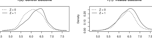
(a) Outcome

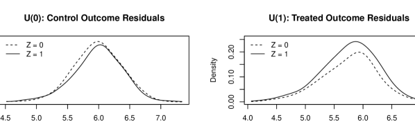
(b) Nesting Inequality Densities

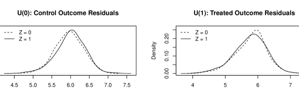
(c) Rewighted

Figure 10: Card (1993) subdensities. 10(a) plots conditional $(Y,D)$ subdensities for $Z=0$ and $Z=1$ where the outcome $Y$ is log weekly earnings. 10(b) and 10(c) plot condidtional subdensities for $(U,D)$, where $U$ are the partial residuals obtained by controlling for residence in the South, residence in a standard metropolitan statistical area in 1966, residence in a standard metropolitan statistical area in 1976, race, potential experience and its square, living in a single mother household at age 14, living with both parents at age 14, father’s and mother’s years of education, indicators for when father’s and mother’s years of indication are missing, a nine value categorical variable constructed by interacting father’s and mother’s education class, and a category for region of residence in 1966. 10(b) are nesting inequality subdensites which are trimmed to ensure first-order stochastic dominance. 10(c) are index sufficiency subdensities which are reweighted by $P(Z=1|p(X,Z))$. Densities use the Gaussian kernel with the rule-of-thumb bandwidth.

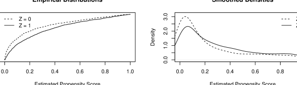
Figure 11: Card (1993) distribution and density of the estimated propensity score. The propensity score is estimated by probit with controls consisting of the instrument, the conditioning covariates, and interactions between the two. Conditioning covariates consist of residence in the South, residence in a standard metropolitan statistical area in 1966, residence in a standard metropolitan statistical area in 1976, race, potential experience and its square, living in a single mother household at age 14, living with both parents at age 14, father’s and mother’s years of education, indicators for when father’s and mother’s years of indication are missing, a nine value categorical variable constructed by interacting father’s and mother’s education class, and a category for region of residence in 1966. The distribution is the simple empirical distribution of estimated propensity scores. The density is an estimated kernel density using the Gaussian kernel and the rule-of-thumb bandwidth.

5.2 Angrist and Evans (1998)

Angrist and Evans (1998) estimate the effect of family size on parental labour supply using the same-sex instrument, which takes a value of one when the two eldest children are the same sex and zero otherwise. Their justification for this instrument is that the sex of children is randomly determined and that there is a parental preference for mixed sex children, so parents whose first two children are the same sex are more likely to have a third. The validity of this instrument was subsequently challenged in Rosenzweig and Wolpin (2000). Using a simple model of labour supply choice, they show that additional restrictions on preferences are needed for this instrument to satisfy the exclusion restriction.

In response to this debate, the validity of the instrument has been tested by Huber (2015) and Mourifié and Wan (2017). In both cases, the Angrist and Evans (1998) sample is split into subgroups based on values of a subset of the covariates, and then instrument validity is tested for each subgroup. Huber (2015) defines 66 subgroups, and finds that the Huber and Mellace (2015) test rejects the null in a small number of them, but the Kitagawa (2015) test never rejects the null. Mourifié and Wan (2017) reports no rejections at the 10% level of significance in 24 subgroups. Neither Huber (2015) or Mourifié and Wan (2017) uses the full set of covariates from the original specification of Angrist and Evans (1998), andsome of the variables that are used are coarsened.

We use the replication files for Angrist and Evans (1998) to construct the sample and variables. We focus on the 1980 Census sample of married mothers. This consists of married mothers aged between 21 and 35 who have at least two children and were at least 15 years old at the time of their first birth. The sample contains 254,652 observations. To keep estimation of the semiparametric model feasible, we use a randomly chosen 1 / 20 subsample of this data, which results in 12,732 observations. $Z$ is the same-sex instrument. $D$ is an indicator set to 1 for mothers with more than two children. Angrist and Evans (1998) presents results for several measures of labour supply. Here we set $Y$ to be the logarithm of annual family labour income. The headline specification controls for demographic characteristics of the mother, the sex of the first child, and the sex of the second child.

Panel 12(a) of Figure 12 plots subdensities for the outcomes without controlling for covariates. In this case there is no visual evidence of violation of the instrument validity. Angrist and Evans (1998) shows that the same-sex instrument almost exactly balances covariate values, which suggests that the instrument and covariates are independent. As discussed in Section 4, when the instrument and covariates are independent, failure to control for covariates can mask violations of instrument validity.

Figure 13 plots the conditional distributions and smoothed densities for the estimated propensity scores. There is no obvious violation of first-order stochastic dominance, and the propensity score densities overlap. One observation is removed when constructing a distilled sample for the test of nesting inequalities. However, as seen in Table 5, only a small fraction of the observations are used in the test of index sufficiency. Since Angrist and Evans (1998) uses only a small number of discrete covariates, there are few estimated propensity score values where there is a mixture of observations with $Z=0$ and $Z=1$. Hence, the estimate of $\Pr(Z=1|p(X,Z))$ is either 0 or 1 for the majority of the sample, and these observations are removed for the test of index sufficiency. Panels 12(b) and 12(c) of Figure 12 plot smoothed subdensities for the samples used in the nesting inequalities with a distilled sample and index sufficiency tests. There is no visual evidence of a violation of the nesting inequalities. For index sufficiency, both the $U(0)$ and $U(1)$ subdensities for $Z=0$ and $Z=1$ appear to differ. However, the results in Table 5 show that this difference is not statistically significant.

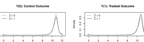
(a) Outcome Densities

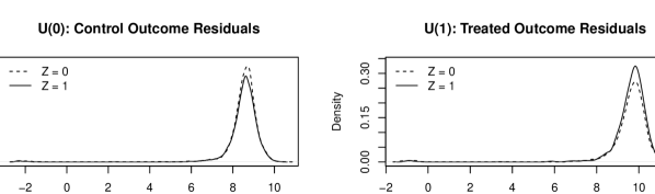
(b) Nesting Inequality Densities

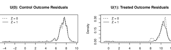
(c) Index Sufficiency Densities

Figure 12: Angrist and Evans (1998) subdensities. 12(a) plots conditional $(Y,D)$ subdensities for $Z=0$ and $Z=1$ where the outcome $Y$ is log annual family earnings. 12(b) and 12(c) plot condidtional subdensities for $(U,D)$, where $U$ are the partial residuals obtained by controlling for mother’s age, mother’s age at the time of the first birth, two dummies for mother’s race, and dummies for the first and second child being a boy. 12(b) are nesting inequality subdensites which are trimmed to ensure first-order stochastic dominance. 12(c) are index sufficiency subdensities which are reweighted by $P(Z=1|p(X,Z))$. Densities use the Gaussian kernel with the rule-of-thumb bandwidth.

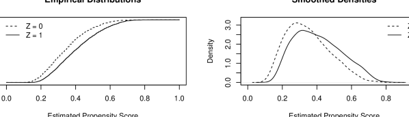
Figure 13: Angrist and Evans (1998) distribution and density of the estimated propensity score. The propensity score is estimated by probit with controls consisting of the instrument, the conditioning covariates, and interactions between the two. Conditioning covariates consist of mother’s current age, mother’s age at the time of the birth of their first child, the sex of the first child, and two dummies for race. The distribution is the simple empirical distribution of estimated propensity scores. The density is an estimated kernel density using the Gaussian kernel and the rule-of-thumb bandwidth.

5.3 Oreopoulos (2006)

Changes in schooling laws have been used as an instrument to estimate the effects of education for a variety of outcomes. Acemoglu and Angrist (2000) uses this instrument to estimate human capital externalities, Lochner and Moretti (2004) estimates effects on crime, Lleras-Muney (2005) effects on health, and Oreopoulos (2006) the returns to education. These designs exploit variation in the timing of changes in compulsory schooling laws across locations. Conditional on covariates, such as location and time fixed effects, this variation is assumed to be unrelated to other changes. Stephens and Yang (2014) presents evidence that this assumption does not hold in data for US states and, in particular, that changes in compulsory schooling laws are correlated with changes in school quality. Brunello et al. (2013) develops a test of uncorrelatedness between changes in compulsory schooling laws and school quality. They apply this test to European data and find that they cannot reject the null of uncorrelatedness. Bolzern and Huber (2017) tests the validity of the compulsory schooling law instrument using the Huber and Mellace (2015) and Kitagawa (2015) tests with data from seven European countries, and does not reject the null of instrument validity.

We apply our test to the data of Oreopoulos (2006). The instrument is the legal minimum school leaving age for the UK. This was increased from 14 to 15 in 1947 in Great Britain and in 1957 in Northern Ireland. The dataset consists of individuals aged between 16 and 65. It is constructed by combining UK and Northern Ireland household surveys for the years 1984 through to 2006. $Y$ is log real earnings, $D$ is age of leaving full-time education, and $Z$ is a dummy for the legal minimum leaving age faced at age 14 being 15. Conditioning covariates are year aged 14, current age, sex, survey year and residence in Northern Ireland. As with Card (1993), the treatment variable must be binarized. Here we define the treatment to be one if the age of leaving education is at least 15. We investigate the possibility that this induces coarsening bias, but the binarised treatment seems to capture well the variation in the underlying treatment induced by the instrument.

The data consists of 82,908 observations which are aggregated into 30,587 cells. Each cell consists of individuals with common values of the treatment, instrument and conditioning covariates. The outcome variable is averaged at the cell level, and each cell is assigned a weight equal to the number of individuals it contains. The identifying assumptions stated in Section 2.2 were not for data that has been aggregated in this way. However, the aggregation procedure preserves all variables apart from the outcome, which implies that the propensity score is also preserved. The identifying assumptions may then be simply restated in terms of the averaged outcome, and the same testable implications derived.

Panel 14(a) of Figure 14 plots subdensities for the outcome variable. It is immediately noticeable that there are very few observations with $Z=1$ and $D=0$. Figure 15 plots the conditional distributions and densities for the propensity score. First-order stochastic dominance clearly holds, but the distributions barely overlap. The estimated $\Pr(Z=1|p(X,Z))$ is either 1 or 0 for all cells. The entire sample is used in the test of nesting inequalities with a distilled sample, but there are no observations for which to perform the test of index sufficiency. Table 5 therefore present p-values for the test of nesting inequalities with a distilled sample only. We find that the null is rejected at even the 1% level of significance. The violation is in the lower tail of the $U(1)$ subdensities, which are plotted in panel 14(b) of Figure 14. The subdensity of $U(1)$ for $Z=0$ does not lie entirely within the support of the subdensity for $Z=1$.

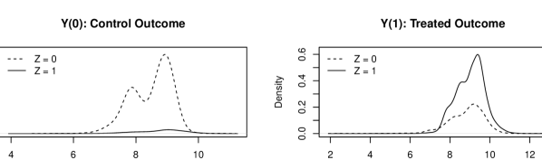
(a) Outcome Densities

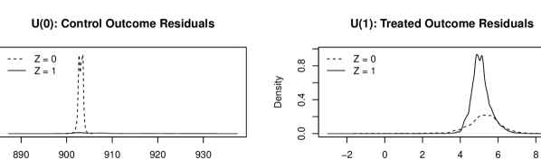
(b) Nesting Inequality Densities

Figure 14: Oreopoulos (2006) subdensities. 14(a) plots conditional $(Y,D)$ subdensities for $Z=0$ and $Z=1$ where the outcome $Y$ is log real earnings. 14(b) plots condidtional subdensities for $(U,D)$, where $U$ are the partial residuals obtained by controlling for year aged 14 fixed effects, a quartic polynomial for current age, sex, survey year fixed effects and residence in Northern Ireland. 14(b) are nesting inequality subdensites which are trimmed to ensure first-order stochastic dominance. Densities use the Gaussian kernel with the rule-of-thumb bandwidth.

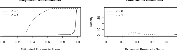
Figure 15: Oreopoulos (2006) distribution and density of the estimated propensity score. The propensity score is estimated by probit with controls consisting of the instrument, the conditioning covariates, and interactions between the two. Conditioning covariates consist of year aged 14 fixed effects, a quartic polynomial for current age, sex, survey year fixed effects and residence in Northern Ireland6. The distribution is the simple empirical distribution of estimated propensity scores. The density is an estimated kernel density using the Gaussian kernel and the rule-of-thumb bandwidth.

6 Conclusion

This paper develops a novel test for instrument validity in the LATE/MTE framework that can accommodate conditioning covariates. We follow Carneiro et al. (2011) in assuming a linear relationship between potential outcomes and conditioning covariates and that unobserved heterogeneities are independent of the instrument and covariates.. Expected outcomes then follow a partially linear model, depending linearly on conditioning covariates and non-parametrically on the propensity score. With this functional form, partial residuals can be obtained by partialing out the conditioning covariates. We derive testable implication for the subdensities of these partial residuals: index sufficiency and the nesting inequalities. We propose a test procedure consisting of an initial step where the partially linear model is estimated and partial residuals obtained, followed by a joint test of index sufficiency and the nesting inequalities. Crucially, as conditioning covariates are partialed out, they increase only the complexity of estimating the propensity score and the partially linear model. In this way, the test procedure overcomes the computational hurdles of implementing tests such as Kitagawa (2015), Huber and Mellace (2015) and Mourifié and Wan (2017) in the presence of conditioning covariates.

The testable implications are complementary. Index sufficiency holds the propensity score fixed and compares subdensities for different values of the instrument, whereas the nesting inequalities are distributional monotonicity relations ordered with respect to the propensity score. A straightforward approach to testing the nesting inequalities is to coarsen the propensity score and check the inequalities for subdensities indexed by this coarsened variable. However, in cases where the propensity score is strongly correlated with the conditioning covaraites, the distribution of instrument values can become homogenised across propensity score bins, leading to a lack of power. We showed that the nesting inequalities hold with the original instrument in place of the propensity score if the conditional distribution of the propensity score given the instrument is stochastically monotonic in the sense of first-order stochastic dominance. Since first-order stochastic dominance is not implied by the identifying assumptions, we proposed testing the nesting inequalities using a trimmed sample where first-order stochastic dominance does hold. We refer to this process as distillation, and present an algorithm for constructing distilled samples. We show analytically a class of data generating processeses where distillation is guaranteed to outperform a test of the nesting inequalities over propensity score bins in terms of detecting violations of instrument validity. Monte Carlo exercises confirm this finding, with consistent gains in power when using the proposed test procedure in place of testing the nesting inequalities with a coarsened propensity score.

We believe that there are two areas which future research could address. First, formal characterisation of the size and power of this test, incorporating uncertainty over estimation of the partial residuals and the distillation process, is left for future research. Second, as noted in Section 2, in general there will be many possible distilled samples that satisfy the first-order stochastic dominance condition. In Proposition 5, we showed a restriction on trimming that is guaranteed to improve detection of violations of instrument validity for a class of data generating processes, and we provided an algorithm that satisfies this restriction. However, other possibilities exist, and the optimal choice of distillation process is an open question.

Appendix

Appendix A Proofs for Propositions 1 and 2

Proof of Proposition 1. Fix the value of the conditioning variable $X$ at $x$, and consider an arbitrary Borel subset $A\subset\mathcal{Y}$.  Then, the additive error representation of the selection equation in (1) implies that the event $\{Y\in A,D=1|X=x,Z=z\}$ is equivalent to $\{Y_{1}\in A,V\leq p|p\left(X,Z\right)=p,X=x,Z=z\}$. We therefore obtain

$$\Pr\left(Y\in A,D=1|X=x,Z=z\right) = \Pr\left(Y_{1}\in A,V\leq p|p\left(X,Z\right)=p,X=x,Z=z\right)$$

$$= \Pr\left(Y_{1}\in A,V\leq p|X=x\right),$$

where the second equality follows from the random assignment condition (A2). Similarly, for $D=0$ case, we have

$$\Pr\left(Y\in A,D=0|X=x,Z=z\right)=\Pr\left(Y_{0}\in A,V>p|X=x\right).$$

These prove index sufficiency, i.e., conditional on $X$, the distribution of $(Y,D)$ depends on $Z$ through the propensity score $p(X,Z)$ only.

To obtain the nesting inequalities, we note

$$\Pr(Y\in A,D=1|p\left(Z,X\right)=p,X=x)-\Pr(Y\in A,D=1|p\left(Z,X\right)=p^{\prime},X=x)$$ (47)

$$= \Pr(Y_{1}\in A,V\leq p|X=x)-\Pr(Y_{1}\in A,V\leq p^{\prime}|X=x)$$

$$= \Pr(Y_{1}\in A,p^{\prime}<V\leq p|X=x)\geq 0,$$

follows. The inequality for $D=0$ case is proven in a similar manner.   

Proof of Proposition 2. Noting that the event $\{U\in A,D=1|X=x,Z=z\}$ is equivalent to $\{U\in A,V\leq p|p(X,Z)=p,X=x,Z=z\}$, we have

$$\Pr\left(U\in A,D=1|X=x,Z=z\right) = \Pr\left(U_{1}\in A,V\leq p|p\left(X,Z\right)=p,X=x,Z=z\right)$$

$$= \Pr\left(U_{1}\in A,V\leq p\right),$$

where the second equality follows from the strong exogeneity condition of (A4). A similar argument gives

$$\Pr\left(U\in A,D=0|X=x,Z=z\right)=\Pr\left(U_{0}\in A,V>p\right)$$

Hence, we obtain index sufficiency: the distribution of $(U,D)$ depends on $(X,Z)$ through the propensity score $p(X,Z)$ only.

To obtain the nesting inequalities, by (8) and recalling that $V$ is uniformly distributed, we have

$$\Pr(U\in A,D=1|p\left(X,Z\right)=p)-\Pr(U\in A,D=1|p\left(X,Z\right)=p^{\prime})$$

$$= \Pr(U_{1}\in A,U_{D}\leq p)-\Pr(U_{1}\in A,U_{D}\leq p^{\prime})$$

$$= \Pr(U_{1}\in A,p^{\prime}<U_{D}\leq p)$$

$$\geq 0.$$ (48)

The other inequality of the proposition can be shown similarly.   

Appendix B Proof of Proposition 5

This section presents a proof for Proposition 5. We first introduce notation, then show several lemmas, and then use these lemmas to prove each of the three statements of Proposition 5. We prove the statements of Proposition 5. for $D=1$. The proof for $D=0$ is identical.

B.1 Notation

Let $P$ be an inerval of propensity scores. Define

$$\mathcal{F}(P,z)\equiv\int_{P}\Pr(U\in A,D=1|p,Z=z)f(p|p\in P,Z=z)dp,$$

$$w(z|P)\equiv\Pr(Z=z|p\in P).$$

The joint probability of $(U\in A,D=1)$ conditional on $p\in P$ may be written as

$$\Pr(U\in A,D=1|p\in P)=(1-w(1|P))\mathcal{F}(P,0)+w(1|P)\mathcal{F}(P,1).$$ (49)

Thus the nesting inequality with a coarsened propensity score, (20), subtracts a weighted sum of $\mathcal{F}(P^{+},0)$ and $\mathcal{F}(P^{+},1)$ from a weighted sum of $\mathcal{F}(P^{-},0)$ and $\mathcal{F}(P^{-},1)$

$$(1-w(1|P^{-}))\mathcal{F}(P^{-},0)+w(1|P^{-})\mathcal{F}(P^{-},1)-(1-w(1|P^{+}))\mathcal{F}(P^{+},0)-w(1|P^{+})\mathcal{F}(P^{+},1).$$ (50)

We refer to (50) as the coarsened propensity score nesting violation.

Define

$$\mathcal{G}(P,z)\equiv\int_{P}\Pr(U\in A,D=1|p,S_{1}=1,Z=z)f(p|p\in P,S_{1}=1,Z=z)dp,$$

$$v(P|z)\equiv\Pr(p\in P|Z=z,S_{1}=1,p\in P^{-}\cup P^{+}).$$

The joint probability of $(U\in A,D=1)$ conditional on $Z=z$, $S_{1}=1$ and $p\in P^{-}\cup P^{+}$ can be written

$$\Pr(U\in A,D=1|Z=z,p\in P^{-}\cup P^{+})=v(P^{-}|z)\mathcal{G}(P^{-},z)+v(P^{+}|z)\mathcal{G}(P^{+},z).$$ (51)

Thus the nesting inequality with a distilled sample, (1), subtracts a weighted sum of $\mathcal{G}(P^{-},1)$ and $\mathcal{G}(P^{+},1)$ from a weighted sum of $\mathcal{G}(P^{-},0)$ and $\mathcal{G}(P^{+},0)$,

$$v(P^{-}|0)\mathcal{G}(P^{-},0)+v(P^{+}|0)\mathcal{G}(P^{+},0)-v(P^{-}|1)\mathcal{G}(P^{-},1)-v(P^{+}|1)\mathcal{G}(P^{+},1).$$ (52)

We refer to (52) as the distilled nesting violation.

B.2 Lemmas

Lemma 6

The labeling condition of Proposition 5 implies

$$w(1|P^{+})\geq w(1|P^{-}).\\$$ (53)

Proof of Lemma 6.

Write out the labeling condition (24) and rearrange

$$\frac{\Pr(Z=1,p\in P^{+})}{\Pr(Z=1,p\in P^{+})+\Pr(Z=1,p\in P^{-})} \geq\frac{\Pr(Z=0,p\in P^{+})}{\Pr(Z=0,p\in P^{-})+\Pr(Z=0,p\in P^{+})}$$

$$\implies\Pr(Z=1,p\in P^{+})\Pr(Z=0,p\in P^{-}) \geq\Pr(Z=1,p\in P^{-})\Pr(Z=0,p\in P^{+})$$

$$\implies\Pr(Z=1,p\in P^{+})\Pr(p\in P^{-}) \geq\Pr(Z=1,p\in P^{-})\Pr(p\in P^{+})$$

$$\implies\Pr(Z=1|p\in P^{+}) \geq\Pr(Z=1|p\in P^{-}).$$

The third line adds $\Pr(Z=1,p\in P^{+})\Pr(Z=1,p\in P^{-})$ to both sides and simplifies. By definition, the left hand side of the last line $w(1|P^{+})$, and the right hand side is $w(1|P^{-})$.  

Lemma 7

The labeling condition and trimming rule jointly imply

$$v(P^{+}|1)\geq v(P^{+}|0).$$ (54)

Proof of Lemma 7.

Consider first $v(P^{+}|1)$

$$v(P^{+}|1) \equiv\frac{\Pr(Z=1,p\in P^{+},S_{1}=1)}{\Pr(Z=1,p\in P^{+},S_{1}=1)+\Pr(Z=1,p\in P^{-},S_{1}=1)}$$

$$=\frac{\Pr(Z=1,p\in P^{+})}{\Pr(Z=1,p\in P^{+})+\Pr(Z=1,p\in P^{-},S_{1}=1)}$$

$$\geq\frac{\Pr(Z=1,p\in P^{+})}{\Pr(Z=1,p\in P^{+})+\Pr(Z=1,p\in P^{-})}$$

The second line uses that the trimming under imposes that all observations with $Z=1$ and $p\in P^{+}$ are retained. The third line follows from $\Pr(Z=1,p\in P^{-})\geq\Pr(Z=1,p\in P^{-},S_{1}=1)\geq 0$. The expression on the last line is equivalent to $\Pr(p\in P^{+}|Z=1)$, hence

$$v(P^{+}|1)\geq\Pr(p\in P^{+}|Z=1)$$ (55)

Following the same steps with $v(P^{+}|0)$, and using that the trimming rule imposes that all observations $Z=0$ and $p\in P^{-}$ are retained yields

$$\Pr(p\in P^{+}|Z=1)\geq v(P^{+}|0)$$ (56)

Combine (55), (56) and the labeling condition (24)

$$v(P^{+}|1)\geq\Pr(p\in P^{+}|Z=1)\geq\Pr(p\in P^{+}|Z=1)\geq v(P^{+}|0)$$

 

Lemma 8

The conditional nesting assumption implies

$$\mathcal{F}(P^{+},z)\geq\mathcal{F}(P^{-},z),$$ (57)

for $z\in\{0,1\}$.

Proof of Lemma 8.

Let $\hat{p}$ be the upper bound of $P^{-}$. Equation (25) implies

$$\mathcal{F}(P^{+},z) \equiv\int_{P^{+}}\Pr(U\in A,D=1|Z=z,p)f(p|p\in P^{+},Z=z)dp$$

$$\geq\Pr(U\in A,D=1|Z=z,p=\hat{p})$$

$$\geq\int_{P^{-}}\Pr(U\in A,D=1|Z=z,p)f(p|p\in P^{-},Z=z)dp$$

$$\equiv\mathcal{F}(P^{-},z).$$

 

Lemma 9

Under the trimming rule

$$\mathcal{G}(P^{-},0)=\mathcal{F}(P^{-},0),$$ (58)

$$\mathcal{F}(P^{+},1)=\mathcal{G}(P^{+},1).$$ (59)

Proof of Lemma 9.

Equation (58) is shown as follows

$$\mathcal{G}(P^{-},0) \equiv\int_{P^{-}}\Pr(U\in A,D=1|p,S_{1}=1,Z=0)f(p|p\in P^{-}S_{1}=1,Z=0)dp,$$

$$=\int_{P^{-}}\Pr(U\in A,D=1|p,Z=0)f(p|p\in P^{-},Z=0)dp$$

$$\equiv\mathcal{F}(P^{-},0).$$

The second line uses that, under the trimming rule, $S_{1}=1$ for all observations with $Z=0$ and $p\in P^{-}$. By using that $S_{1}=1$ for all observations with $Z=1$ and $p\in P^{+}$, (59) can be shown similarly.   

Lemma 10

The conditional nesting assumption and trimming rule jointly imply

$$\mathcal{G}(P^{+},1)\geq\mathcal{G}(P^{-},1),$$ (60)

and either

$$\mathcal{G}(P^{+},0) \geq\mathcal{G}(P^{-},0),$$ (61)

$$v(P^{+},0) >0,$$ (62)

or

$$\mathcal{G}(P^{+},0)=0,$$ (63)

$$v(P^{+},0)=0.$$ (64)

Proof of Lemma 10.

To show (60), use Lemma 9 to impose $\mathcal{F}(P^{+},1)=\mathcal{G}(P^{+},1)$. The inequality can then be shown by following the proof for Lemma 8.

For (61) and (63), note that under the trimming rule it is possible that all observations with $Z=0,p\in P^{+}$ are trimmed. If the trimmed sample includes observations with $Z=0,p\in P^{+}$, then $\Pr(p\in P^{+},Z=1,S_{1}=1)>0$, which implies (62). Equation (61) can ten be shown by following the proof for Lemma 8. If all observations with $Z=0,p\in P^{+}$ are trimmed, then $\Pr(p\in P^{+},Z=1,S_{1}=1)=0$, and (63) and (64) follow immediately.   

B.3 Proof of Proposition 5

Proof of Statement 1.

Suppose that the coarsened propensity score nesting violation (50) is positive. For a weighted sum of $\mathcal{F}(P^{-},0)$ and $\mathcal{F}(P^{-},1)$ to exceed a weighted sum of $\mathcal{F}(P^{+},0)$ and $\mathcal{F}(P^{+},1)$, it must be that

$$\text{max}(\mathcal{F}(P^{-},0),\mathcal{F}(P^{-},1))>\text{min}(\mathcal{F}(P^{+},0),\mathcal{F}(P^{+},1)).$$ (65)

Combining (65) and Lemma 8, there are two possible orderings of $\mathcal{F}(P^{+},0)$, $\mathcal{F}(P^{-},0)$, $\mathcal{F}(P^{+},1)$, and $\mathcal{F}(P^{-},1)$

$$\mathcal{F}(P^{-},0)\leq\mathcal{F}(P^{+},0)\leq\mathcal{F}(P^{-},1)\leq\mathcal{F}(P^{+},1),$$ (66)

$$\mathcal{F}(P^{-},1)\leq\mathcal{F}(P^{+},1)\leq\mathcal{F}(P^{-},0)\leq\mathcal{F}(P^{+},0).$$ (67)

Rewrite (50) as

$$w(1|P^{-})(\mathcal{F}(P^{-},1)-\mathcal{F}(P^{+},1))+(1-w(1|P^{-}))(\mathcal{F}(P^{-},0)-\mathcal{F}(P^{+},0))\\ -(w(1|P^{+})-w(1|P^{-}))(\mathcal{F}(P^{+},1)-\mathcal{F}(P^{+},0)).$$ (68)

Lemma 8 implies that the first two terms are (weakly) negative. Turning to the final term, by Lemma 6

$$w(1|P^{+})-w(1|P^{-})\geq 0,$$

If (66) holds, $\mathcal{F}(P^{+},1)>\mathcal{F}(P^{+},0)$, and this last term will also be negative, which implies that the nesting inequality for a coarsened propensity can never be positive. Hence, for this nesting inequality to be positive, (67) must hold.

Assuming (67) holds, we obtain the inequality

$$v(P^{+}|0)\mathcal{G}(P^{+},0)+v(P^{-}|0)\mathcal{G}(P^{-},0) \geq\mathcal{F}(P^{-},0)$$

$$\geq(1-w(1|P^{-}))\mathcal{F}(P^{-},0)+w(1|P^{-})\mathcal{F}(P^{-},1).$$ (69)

The first inequality holds by Lemma 9 and Lemma 10. The second inequality follows directly from (67). Maintaining (67), we can obtain the additional inequality

$$(1-w(1|P^{+}))\mathcal{F}(P^{+},0)+w(1|P^{+})\mathcal{F}(P^{+},1) \geq\mathcal{F}(P^{+},1)$$

$$\geq v(P^{+}|1)\mathcal{G}(P^{+},1)+v(P^{-}|1)\mathcal{G}(P^{-},1).$$ (70)

Here the first inequality follows from (67), while the second uses Lemma 9 and Lemma 10.

Summing (69) and (70)

$$v(P^{+}|0)\mathcal{G}(P^{+},0)+v(P^{-}|0)\mathcal{G}(P^{-},0)+(1-w(1|P^{+}))\mathcal{F}(P^{+},0)+w(1|P^{+})\mathcal{F}(P^{+},1)\geq\\ (1-w(1|P^{-}))\mathcal{F}(P^{-},0)+w(1|P^{-})\mathcal{F}(P^{-},1)+v(P^{+}|1)\mathcal{G}(P^{+},1)+v(P^{-}|1)\mathcal{G}(P^{-},1),$$

which can be rearranged to

$$v(P^{+}|0)\mathcal{G}(P^{+},0)+v(P^{-}|0)\mathcal{G}(P^{-},0)-v(P^{+}|1)\mathcal{G}(P^{+},1)-v(P^{-}|1)\mathcal{G}(P^{-},1)\geq\\ (1-w(1|P^{-}))\mathcal{F}(P^{-},0)+w(1|P^{-})\mathcal{F}(P^{-},1)-(1-w(1|P^{+}))\mathcal{F}(P^{+},0)-w(1|P^{+})\mathcal{F}(P^{+},1).$$

The left-hand side is the distilled nesting violation (52). The right-hand side is the coarsened propensity score nesting violation (50).

 

Proof of Statement 2.

Our strategy to show the second statement is as follows. First, we make assumptions such that, for a given $A$, the coarsened propensity score nesting violation (50) is not positive. We then show that this does not preclude the distilled nesting violation (52) from being positive.

The above argument established that (67) must hold for the nesting inequality conditional on bins of $p$ to be positive. Therefore, to guarantee that the nesting inequality conditional on the coarsened propensity score is negative, we assume that (67) does not hold i.e.

$$\mathcal{F}(P^{-},0)<\mathcal{F}(P^{+},1).$$ (71)

Write the distilled nesting violation (52) as

$$v(P^{-}|1)(\mathcal{G}(P^{-},0)-\mathcal{G}(P^{-},1))+(v(P^{-}|0)-v(P^{-}|1))(\mathcal{G}(P^{-},0)-\mathcal{G}(P^{+},1))\\ +(1-v(P^{-}|0))(\mathcal{G}(P^{+},0)-\mathcal{G}(P^{+},1)).$$ (72)

Expressed this way, (52) is a weighted sum of the differences $\mathcal{G}(P^{-},0)-\mathcal{G}(P^{-},1)$, $\mathcal{G}(P^{-},0)-\mathcal{G}(P^{+},1)$ and $\mathcal{G}(P^{+},0)-\mathcal{G}(P^{+},1)$. Lemma 7 guarantees that $v(P^{-}|0)-v(P^{-}|1)\geq 0$, so the weights are all (weakly) positive. By Lemma 9, (71) is equivalent to

$$\mathcal{G}(P^{-},0)<\mathcal{G}(P^{+},1).$$ (73)

Assuming (73), (72) can only be positive if at least one of $\mathcal{G}(P^{-},0)-\mathcal{G}(P^{-},1)$ and $\mathcal{G}(P^{+},0)-\mathcal{G}(P^{+},1)$ is positive.

Take the four $\mathcal{G}(P,z)$ as given and solve for $v(P^{-}|0)$ and $v(P^{-}|1)$ such that (72) is positive subject to the constraints

$$0\leq v(P^{-}|0)\leq 1,$$

$$0\leq v(P^{-}|1)\leq 1,$$

$$v(P^{-}|1)\leq v(P^{-}|0).$$

Doing so yields the following bounds for $v(P^{-}|0)$

$$v(P^{-}|1)\leq v(P^{-}|0)\leq\text{min}\left\{1,\frac{v(P^{-},1)(\mathcal{G}(P^{+},1)-\mathcal{G}(P^{-},1))+\mathcal{G}(P^{+},0)-\mathcal{G}(P^{+},1)}{\mathcal{G}(P^{+},0)-\mathcal{G}(P^{-},0)}\right\}.$$ (74)

and for $v(P^{-}|1)$

$$\mathbbm{1}\left\{\mathcal{G}(P^{+},0)\leq\mathcal{G}((P^{+},1)\right\}\bar{v}\leq v(P^{-}|1)\leq 1-\mathbbm{1}\left\{\mathcal{G}(P^{-},0)\leq\mathcal{G}(P^{-},1)\right\}(1+\bar{v}).$$ (75)

with

$$\bar{v}\equiv\frac{\mathcal{G}(P^{+},1)-\mathcal{G}(P^{+},0)}{\mathcal{G}(P^{+},1)-\mathcal{G}(P^{-},1)-\mathcal{G}(P^{+},0)+\mathcal{G}(P^{-},0)}.$$

Taking $v(P^{-}|1)$ as given, (74) gives bounds for $v(P^{-}|0)$ such that (72) is positive. Equation (75) gives bounds for $v(P^{-}|1)$ such that the bounds in (74) are non-empty. If $\mathcal{G}(P^{-},0)\geq\mathcal{G}(P^{-},1)$ and $\mathcal{G}(P^{+},0)\geq\mathcal{G}(P^{+},1)$, for any $v(P^{-}|1)$ between 0 and 1 there exists $v(P^{-}|0)$ such that (72) is positive. If $\mathcal{G}(P^{-},0)\geq\mathcal{G}(P^{-},1)$ and $\mathcal{G}(P^{+},0)\leq\mathcal{G}(P^{+},1)$, a $v(P^{-}|0)$ where (72) is positive exists if $v(P^{-}|1)$ is above $\bar{v}$. If $\mathcal{G}(P^{-},0)\leq\mathcal{G}(P^{-},1)$ and $\mathcal{G}(P^{+},0)\geq\mathcal{G}(P^{+},1)$, a $v(P^{-}|0)$ where (72) is positive exists if $v(P^{-}|1)$ is below $-\bar{v}$.   

Proof of Statement 3.

To prove the third statement, we first find a sufficient condition for the coarsened propensity score nesting violation (50) to be negative for any $A$. We then show that it is possible to construct a process where this condition holds and the distilled nesting violation (52) is positive.

Consider again (50). Lemma 6 and Lemma 8 together imply

$$w(1|P^{-})\mathcal{F}(P^{-},1)\leq w(1|P^{+})\mathcal{F}(P^{+},1).$$

A sufficient condition for (50) to be negative for a given $A$ is then

$$(1-w(1|P^{-}))\mathcal{F}(P^{-},0)\leq(1-w(1|P^{+}))\mathcal{F}(P^{+},0).$$

and a sufficient condition for (50) to be negative for all $A$ where $\mathcal{F}(P^{+},0)>0$ is

$$\underset{A}{\text{sup}}\left\{\frac{\mathcal{F}(P^{-},0)}{\mathcal{F}(P^{+},0)}\right\}\leq\frac{1-w(1|P^{+})}{1-w(1|P^{-})}.$$ (76)

Note that Lemma 8 implies the left-hand side is weakly below 1. Hence (76) will always hold if $w(1|P^{+})=w(1|P^{-})$. That is, if the mixture of $Z=0$ and $Z=1$ observations is sufficiently similar in $P^{-}$ and $P^{+}$, then (50) will never be positive.

Now consider the distilled nesting violation (52). Assume that (67) holds. Lemmas 7, 8, 9 and 10 together imply

$$v(P^{-}|0)\mathcal{G}(P^{-},0)\geq v(P^{-}|1)\mathcal{G}(P^{-},1).$$

A sufficient condition for (52) to be positive at a given $A$ is

$$v(P^{+}|0)\mathcal{G}(P^{+},0)\geq v(P^{+}|1)\mathcal{G}(P^{+},1).$$

A sufficient condition for (52) to be positive for some $A$ where $\mathcal{G}(P^{+},1)>0$ is thus

$$\underset{A}{\text{sup}}\left\{\frac{\mathcal{G}(P^{+},0)}{\mathcal{G}(P^{+},1)}\right\}\geq\frac{v(P^{+}|1)}{v(P^{+}|0)}.$$ (77)

For any $A$ where (67) holds, the left-hand side is bounded from below by 1. Equation (77) thus states that, if (67) holds for some $A$ and the mixture of observations from $P^{-}$ and $P^{+}$ is sufficiently similar for $Z=0$ and $Z=1$, then (52) is positive for that $A$.

A case where (76) and (77) are immediate is when there exists $A$ such that $\mathcal{G}(P^{+},0)>\mathcal{G}(P^{+},1)$ and $Z$ is an irrelevant instrument that is independent of $X$. Then

$$w(1|P^{+}) =w(1|P^{-}),$$

$$v(P^{+}|1) =v(P^{+}|0).$$

Hence, any violation can only be detected by conditioning on $Z$.   

Appendix C Numerical Example

This section derives properties of the conditional joint densities of partial residuals and treatment assignment for the process introduced in Section 2.5.

Let $\tilde{\theta}_{1}$ and $\tilde{\theta}_{0}$ be the asymptotic bias of the estimates of $\theta_{1}$ and $\theta_{0}$

$$\tilde{\theta}_{1} =\hat{\theta}_{1}^{*}-\theta_{1},$$

$$\tilde{\theta}_{0} =\hat{\theta}_{0}^{*}-\theta_{0}.$$

Using this notation , the asymptotic partial residuals are

$$U=\nu Z-\nu(1-Z)+D(\bar{U}_{1}-X^{\prime}\tilde{\theta}_{1})+(1-D)(\bar{U}_{0}-X^{\prime}\tilde{\theta}_{0}).$$

Given process of Section 2.5, the following expressions can be derived for the joint density of $(U,D=1)$ conditional on $p$ and $Z$

$$f(U=u,D=1|p,Z=1)=\int_{-\Phi^{-1}(p)}^{\infty}\phi(U_{D})\frac{1}{\sqrt{2\pi\sigma_{\hat{U}_{1}|U_{D},Z=1}^{2}}}\text{exp}\left(-\frac{\left(u-\nu-\mu_{\tilde{U}_{1}|U_{D}}(U_{D})-\frac{\delta_{1}^{\prime}\tilde{\theta_{1}}}{\delta_{1}^{\prime}\delta_{1}}X^{\prime}\delta_{1}\right)^{2}}{2\sigma_{\hat{U}_{1}|U_{D},Z=1}^{2}}\right)dU_{D},$$

$$f(U=u,D=1|p,Z=0)=\int_{-\Phi^{-1}(p)}^{\infty}\phi(U_{D})\frac{1}{\sqrt{2\pi\sigma_{\hat{U}_{1}|U_{D},Z=0}^{2}}}\text{exp}\left(-\frac{\left(u+\nu-\mu_{\tilde{U}_{1}|U_{D}}(U_{D})-\frac{\delta_{0}^{\prime}\tilde{\theta_{1}}}{\delta_{0}^{\prime}\delta_{0}}X^{\prime}\delta_{0}\right)^{2}}{2\sigma_{\hat{U}_{1}|U_{D},Z=0}^{2}}\right)dU_{D}.$$

where $\phi(\cdot)$ is the standard univariate normal density and

$$\mu_{\tilde{U}_{1}|U_{D}}(U_{D})=\mu_{1}+\sigma_{1}\rho_{D,1}U_{D},$$

$$\sigma_{\hat{U}_{1}|U_{D},Z=1}^{2}=\sigma_{1}^{2}(1-\rho_{D,1}^{2})+\left(1-\frac{(\tilde{\theta}_{1}^{\prime}\delta_{1})^{2}}{\tilde{\theta}_{1}^{\prime}\tilde{\theta}_{1}\delta^{\prime}\delta}\right)\tilde{\theta}_{1}^{\prime}\tilde{\theta}_{1},$$

$$\sigma_{\hat{U}_{1}|U_{D},Z=0}^{2}=\sigma_{1}^{2}(1-\rho_{D,1}^{2})+\left(1-\frac{(\tilde{\theta}_{1}^{\prime}\delta_{0})^{2}}{\tilde{\theta}_{1}^{\prime}\tilde{\theta}_{1}\delta^{\prime}\delta}\right)\tilde{\theta}_{1}^{\prime}\tilde{\theta}_{1},$$

with

$$X^{\prime}\delta_{1} =\Phi^{-1}(p)-\alpha,$$ (78)

$$X^{\prime}\delta_{0} =\Phi^{-1}(p)+\alpha.$$ (79)

The expressions for the conditional joint densities of $(U,D=0)$ are analogous. If the asymptotic estimates are unbiased (i.e. $\tilde{\theta}_{1}=0$), then the propensity score only enters through the lower bound of each integral. The derivative of the joint density with respect to $p$ is then weakly positive for all $A$ and $p$ and both $Z=0$ and $Z=1$. Condition (iv) of Proposition 5 must then hold for any non-overlapping intervals of $p$ we consider. However, if $\tilde{\theta}_{1}\neq 0$, there is an additional effect through (78) and (79), changing $p$ affects $X^{\prime}\delta_{1}$ and $X^{\prime}\delta_{0}$. Intuitively, with biased estimates, partialling out does not remove the effect of covariates from the residuals. Changing propensity scores changes the distribution of covariates, which shifts the distribution of partial residuals.

$X^{\prime}\delta_{1}$ and $X^{\prime}\delta_{0}$ enter the density multiplied by $\tilde{\theta}_{1}^{\prime}\delta_{1}$ and $\tilde{\theta}_{1}^{\prime}\delta_{0}$ respectively. Rather than characterising $\tilde{\theta}_{1}$, we characterise these quantities. The following proposition holds

Proposition 11

Consider the terms $\delta_{1}^{\prime}\tilde{\theta}_{1}$, $\delta_{0}^{\prime}\tilde{\theta}_{1}$, $\delta_{1}^{\prime}\tilde{\theta}_{0}$ and $\delta_{0}^{\prime}\tilde{\theta}_{0}$. Assume
(i) The partially linear model is estimated as described in Section 3.1.1.
(ii) The propensity score function $p(X,Z)$ and the conditional expectations $E[X|p(X,Z)]$ and $E[Y|p(X,Z)]$ are consistently estimated.
(iii) There is no perfect multicollinearity among the components of $X-E[X|p(X,Z)]$.
(iv) The matrix $E$ defined in (114) and the matrix $G$ defined in (134) are invertible.
Then

1. The following equalities hold

   $$\tilde{\theta}_{1}^{\prime}\delta_{1}=\tilde{\theta}_{0}^{\prime}\delta_{0},$$

   $$\tilde{\theta}_{0}^{\prime}\delta_{1}=\tilde{\theta}_{1}^{\prime}\delta_{0}.$$

2. $\tilde{\theta}_{1}^{\prime}\delta_{1}$ and $\tilde{\theta}_{1}^{\prime}\delta_{0}$ have the form

   $$\tilde{\theta}_{1}^{\prime}\delta_{1} =\mathcal{H}_{1}(\alpha,\rho_{\delta},\delta^{\prime}\delta)\nu,$$

   $$\tilde{\theta}_{1}^{\prime}\delta_{0} =\mathcal{H}_{0}(\alpha,\rho_{\delta},\delta^{\prime}\delta)\nu.$$

where $\mathcal{H}_{1}$ and $\mathcal{H}_{0}$ are functions. In the numerical exercise, the matrices introduced in assumption (iv) are always invertible. The first statement implies that the coefficients for $X^{\prime}\delta_{1}$ and $X^{\prime}\delta_{0}$ in the subdensities for $(U,D=0)$ will mirror those in the subdensities for $(U,D=1)$, so it is sufficient to only examine one set of subdensities. The second statement implies that, once we have fixed $\nu,\alpha,\delta^{\prime}\delta$ and $\rho_{\delta}$, the actual values of $\delta_{0}$ and $\delta_{1}$ and all other parameters are irrelevant.

C.1 Proof of Proposition 11

The proof proceeds as follows. First, we state several properties of density of the propensity score and the conditional density of $X$ given the propensity score. These properties are then used to show a series of lemmas. Finally, the lemmas are used to show the two statements of Proposition 11.

C.1.1 Propensity Score Density

The propensity score function for this process is

$$p(X,Z)=\Phi(Z(X^{\prime}\delta_{1}+\alpha)+(1-Z)(X^{\prime}\delta_{0}-\alpha)).$$ (80)

Given the distributions of $X$ and $Z$, and this propensity score function, the joint density of $p$ and $Z$ is

$$f(p,Z=0) =\frac{1}{2}\frac{1}{\sqrt{2\pi\delta^{\prime}\delta}}\text{exp}\left(-\frac{(\Phi^{-1}(p)+\alpha)^{2}}{2\delta^{\prime}\delta}\right)\frac{1}{\phi(\Phi^{-1}(p))},$$ (81)

$$f(p,Z=1) =\frac{1}{2}\frac{1}{\sqrt{2\pi\delta^{\prime}\delta}}\text{exp}\left(-\frac{(\Phi^{-1}(p)-\alpha)^{2}}{2\delta^{\prime}\delta}\right)\frac{1}{\phi(\Phi^{-1}(p))}.$$ (82)

Summing (81) and (82), the unconditional density of the propensity score is

$$f(p)=\frac{1}{\sqrt{2\pi\delta^{\prime}\delta}}\text{exp}\left(-\frac{\Phi^{-1}(p)^{2}+\alpha^{2}}{2\delta^{\prime}\delta}\right)\text{cosh}\left(\frac{\Phi^{-1}(p)\alpha}{\delta^{\prime}\delta}\right)\frac{1}{\phi(\Phi^{-1}(p))}.$$ (83)

Notice that this density satisfies

$$f(p)=f(1-p),$$ (84)

which implies

$$\int_{0}^{1}p^{2}f(p)dp=\int_{0}^{1}(1-p)^{2}f(p)dp.$$ (85)

Combining (82) and (83), the probability of $Z=1$ conditional on the propensity score is

$$\Pr(Z=1|p)=\frac{1}{2}+\frac{\text{tanh}(\alpha\Phi^{-1}(p)/\delta^{\prime}\delta)}{2},$$ (86)

which satisfies

$$\Pr(Z=1|p)=1-\Pr(Z=1|1-p).$$ (87)

The symmetry relations (84) and (87), and $\Pr(Z=0|p)=1-\Pr(Z=1|p)$ together imply

$$\int_{0}^{1}p^{2}\Pr(Z=1|p)f(p)dp=\int_{0}^{1}(1-p)^{2}\Pr(Z=0|p)f(p)dp,$$ (88)

$$\int_{0}^{1}p^{2}\Pr(Z=0|p)f(p)dp=\int_{0}^{1}(1-p)^{2}\Pr(Z=1|p)f(p)dp,$$ (89)

$$\int_{0}^{1}p(1-p)\Pr(Z=1|p)f(p)dp=\int_{0}^{1}p(1-p)\Pr(Z=0|p)f(p)dp,$$ (90)

$$\int_{0}^{1}p\Pr(z=0|p)\Pr(z=1|p)f(p)dp=\int_{0}^{1}(1-p)\Pr(z=0|p)\Pr(z=1|p)f(p)dp,$$ (91)

$$\int_{0}^{1}p^{2}\Pr(Z=0|p)\Pr(Z=1|p)f(p)dp=\int_{0}^{1}(1-p)^{2}\Pr(Z=0|p)\Pr(Z=1|p)f(p)dp.$$ (92)

Finally, as $\Phi^{-1}(p)=-\Phi^{-1}(1-p)$ and $\Phi^{-1}(p)^{2}=\Phi^{-1}(1-p)^{2}$

$$\int_{0}^{1}p(1-p)\Pr(Z=1|p)\Pr(Z=0|p)\Phi^{-1}(p)f(p)dp=0,$$ (93)

$$\int_{0}^{1}(1-p)\Pr(z=0|p)\Pr(z=1|p)\Phi^{-1}(p)f(p)dp=-\int_{0}^{1}p\Pr(z=0|p)\Pr(z=1|p)\Phi^{-1}(p)f(p)dp,$$ (94)

$$\int_{0}^{1}p^{2}\Pr(Z=0|p)\Pr(Z=1|p)\Phi^{-1}(p)f(p)dp=-\int_{0}^{1}(1-p)^{2}\Pr(Z=0|p)\Pr(Z=1|p)\Phi^{-1}(p)f(p)dp,$$ (95)

$$\int_{0}^{1}p^{2}\Pr(Z=0|p)\Pr(Z=1|p)\Phi^{-1}(p)^{2}f(p)dp=\int_{0}^{1}(1-p)^{2}\Pr(Z=0|p)\Pr(Z=1|p)\Phi^{-1}(p)^{2}f(p)dp.$$ (96)

Notice that the only parameters which enter the propensity score density and conditional distribution of $Z$ are $\alpha$ and $\delta^{\prime}\delta$. As a consequence, these are the only parameters which affect the integrals above.

C.1.2 Conditional Density of $X$

Given the propensity score function (80), conditioning on $(p,Z=1)$ is equivalent to conditioning on $X^{\prime}\delta_{1}=\Phi^{-1}(p)-\alpha$, and conditioning on $(p,Z=0)$ is equivalent to conditioning on $X^{\prime}\delta_{0}=\Phi^{-1}(p)+\alpha$. Using that $X$ is normally distributed

$$E[X|p,Z=1]=E[X|X^{\prime}\delta_{1}=\Phi^{-1}(p)-\alpha]=\frac{\delta_{1}}{\delta^{\prime}\delta}(\Phi^{-1}(p)-\alpha),$$ (97)

$$E[X|p,Z=0]=E[X|X^{\prime}\delta_{0}=\Phi^{-1}(p)+\alpha]=\frac{\delta_{0}}{\delta^{\prime}\delta}(\Phi^{-1}(p)+\alpha),$$ (98)

$$E[X|p]=\Pr(Z=1|p)\frac{\delta_{1}}{\delta^{\prime}\delta}(\Phi^{-1}(p)-\alpha)+\Pr(Z=0|p)\frac{\delta_{0}}{\delta^{\prime}\delta}(\Phi^{-1}(p)+\alpha).$$ (99)

Let

$$\text{Cov}(X-E[X|p,Z]|p,Z)\equiv E\left[(X-E[X|p,Z])(X-E[X|p,Z])^{\prime}|p,Z\right],\\$$

then

$$\text{Cov}(X-E[X|p,Z]|p,Z=1) =\text{Cov}(X-E[X|p,Z]|X^{\prime}\delta_{1}=\Phi^{-1}(p)-\alpha)=I-\frac{\delta_{1}\delta_{1}^{\prime}}{\delta^{\prime}\delta},$$ (100)

$$\text{Cov}(X-E[X|p,Z]|p,Z=0) =\text{Cov}(X-E[X|p,Z]|X^{\prime}\delta_{0}=\Phi^{-1}(p)+\alpha)=I-\frac{\delta_{0}\delta_{0}^{\prime}}{\delta^{\prime}\delta}.$$ (101)

Similarly, define

$$\text{Cov}(X-E[X|p]|p)\equiv E[(X-E[X|p])(X-E[X|p])^{\prime}|p].$$

$\text{Cov}(X-E[X|p]|p)$ satisfies the decomposition

$$\text{Cov}(X-E[X|p]|p)=E[\text{Cov}(X-E[X|p,Z]|p,Z)|p]+E[\text{Cov}(E[X|p,Z]-E[X|p]|p,Z)|p].$$

Using (97), (98), (99), (100) and (101) and simplifying

$$\text{Cov}(X-E[X|p]|p)=I-\Pr(Z=1|p)\frac{\delta_{1}\delta_{1}^{\prime}}{\delta^{\prime}\delta}-\Pr(Z=0|p)\frac{\delta_{0}\delta_{0}^{\prime}}{\delta^{\prime}\delta}\\ +\frac{\delta_{1}\delta_{1}^{\prime}}{(\delta^{\prime}\delta)^{2}}(\Phi^{-1}(p)-\alpha)^{2}-\frac{\delta_{0}\delta_{1}^{\prime}+\delta_{1}\delta_{0}^{\prime}}{(\delta^{\prime}\delta)^{2}}(\Phi^{-1}(p)-\alpha)(\Phi^{-1}(p)+\alpha)+\frac{\delta_{0}\delta_{0}^{\prime}}{(\delta^{\prime}\delta)^{2}}(\Phi^{-1}(p)+\alpha)^{2}.$$ (102)

C.1.3 Lemmas

Let $\mathbf{X}$ be a column vector of length $2k_{X}$ which stacks $p(X-E[X|p])$ and $(1-p)(X-E[X|p])$. Let $\mathbf{Z}\equiv Z-E[Z|p]$.

Lemma 12

$$E[\mathbf{X}\mathbf{Z}]=\begin{pmatrix}w_{1}\delta_{1}+w_{0}\delta_{0}\\ w_{1}\delta_{0}+w_{0}\delta_{1}\end{pmatrix},$$

where $w_{0}$ and $w_{1}$ are scalars that depend on $\alpha$ and $\delta^{\prime}\delta$ only.

Lemma 13

$$E[\mathbf{X}\mathbf{X}^{\prime}]^{-1}=\begin{pmatrix}\Omega_{1}&\Omega_{2}\\ \Omega_{2}^{\prime}&\Omega_{3}\end{pmatrix},$$

where $\Omega_{1}$, $\Omega_{2}$, and $\Omega_{3}$ are $K\times K$ matrices.

Lemma 14

The following equalities hold

$$\delta_{1}^{\prime}\Omega_{1}\delta_{1}=\delta_{0}^{\prime}\Omega_{3}\delta_{0},$$

$$\delta_{0}^{\prime}\Omega_{1}\delta_{0}=\delta_{1}^{\prime}\Omega_{3}\delta_{1},$$

$$\delta_{0}^{\prime}\Omega_{1}\delta_{1}=\delta_{1}^{\prime}\Omega_{3}\delta_{0},$$

$$\delta_{1}^{\prime}\Omega_{1}\delta_{0}=\delta_{0}^{\prime}\Omega_{3}\delta_{1},$$

$$\delta_{1}^{\prime}\Omega_{2}\delta_{1}=\delta_{0}^{\prime}\Omega_{2}^{\prime}\delta_{0}.$$

Lemma 15

The constants $\delta_{i}^{\prime}\Omega_{k}\delta_{j}$ for $i,j=\{0,1\}$, $k=\{1,2,3\}$ depend on $\alpha$, $\delta^{\prime}\delta$ and $\rho_{\delta}$ only.

Proof of Lemma 12.

$$E[\mathbf{X}\mathbf{Z}] =\begin{pmatrix}E[p(X-E[X|p])(Z-E[Z|p]]\\ E[(1-p)(X-E[X|p])(Z-E[Z|p]]\end{pmatrix},$$

$$=\begin{pmatrix}\int_{0}^{1}p\Pr(z=0|p)\Pr(z=1|p)(E[X|p,Z=1]-E[X|p,Z=0])f(p)dp\\ \int_{0}^{1}(1-p)\Pr(z=0|p)\Pr(z=1|p)(E[X|p,Z=1]-E[X|p,Z=0])f(p)dp\end{pmatrix},$$

$$=\frac{1}{\delta^{\prime}\delta}\begin{pmatrix}\int_{0}^{1}p\Pr(z=0|p)\Pr(z=1|p)(\delta_{1}(\Phi^{-1}(p)-\alpha)-\delta_{0}(\Phi^{-1}(p)+\alpha))f(p)dp\\ \int_{0}^{1}(1-p)\Pr(z=0|p)\Pr(z=1|p)(\delta_{1}(\Phi^{-1}(p)-\alpha)-\delta_{0}(\Phi^{-1}(p)+\alpha))f(p)dp\end{pmatrix},$$

$$=\begin{pmatrix}w_{1}\delta_{1}+w_{0}\delta_{0}\\ w_{1}\delta_{0}+w_{0}\delta_{1}\end{pmatrix},$$ (103)

where $w_{1}$ and $w_{0}$ are the scalars

$$w_{1} =\frac{\int_{0}^{1}p\Pr(z=0|p)\Pr(z=1|p)(\Phi^{-1}(p)-\alpha)f(p)dp}{\delta^{\prime}\delta},$$

$$w_{0} =-\frac{\int_{0}^{1}p\Pr(z=0|p)\Pr(z=1|p)(\Phi^{-1}(p)+\alpha)f(p)dp}{\delta^{\prime}\delta}.$$

The first line uses the definitions of $\mathbf{X}$ and $\mathbf{Z}$. The second line uses the law of iterated expectations, and the $Z$ is binary so $E[Z|p]=\Pr(Z=1|p)$. The third uses (97) and (98). Equations (91) and (94) are used in the fourth.

$w_{1}$ and $w_{0}$ are integrals of functions that depend on $\alpha$ and $\delta^{\prime}\delta$ only. Hence, they themselves will depend on $\alpha$ and $\delta^{\prime}\delta$ only.   

C.1.4 Characterising $E[\mathbf{X}\mathbf{X}^{\prime}]$

By definition

$$E[\mathbf{X}\mathbf{X}^{\prime}]=\begin{pmatrix}E[p^{2}(X-E[X|p])(X-E[X|p])^{\prime}]&E[p(1-p)(X-E[X|p])(X-E[X|p])^{\prime}]\\ E[p(1-p)(X-E[X|p])(X-E[X|p])^{\prime}]&E[(1-p)^{2}(X-E[X|p])(X-E[X|p])^{\prime}]\end{pmatrix}.$$

All four components of this matrix can be written in the form $E[p^{i}(1-p)^{j}(X-E[X|p])(X-E[X|p])^{\prime}]$ where $i$ and $j$ take values $\{0,1,2\}$. Notice that

$$E[p^{i}(1-p)^{j}(X-E[X|p])(X-E[X|p])^{\prime}] =\int_{0}^{1}p^{i}(1-p)^{j}E[(X-E[X|p])(X-E[X|p])^{\prime}|p]f(p)dp,$$

$$=\int_{0}^{1}p^{i}(1-p)^{j}\text{Cov}(X-E[X|p]|p)f(p)dp.$$

Using (102) to substitute for $\text{Cov}(X-E[X|p]|p)$, we can obtain

$$E[\mathbf{X}\mathbf{X}^{\prime}]=\begin{pmatrix}\Psi_{1}&\Psi_{2}\\ \Psi_{2}&\Psi_{3}\end{pmatrix},$$ (104)

$$\Psi_{1}=Ia_{1}+\delta_{1}\delta_{1}^{\prime}a_{2}+\delta_{0}\delta_{0}^{\prime}a_{3}+(\delta_{0}\delta_{1}^{\prime}+\delta_{1}\delta_{0}^{\prime})a_{4},$$

$$\Psi_{3}=Ia_{1}+\delta_{1}\delta_{1}^{\prime}a_{3}+\delta_{0}\delta_{0}^{\prime}a_{2}+(\delta_{0}\delta_{1}^{\prime}+\delta_{1}\delta_{0}^{\prime})a_{4},$$

$$\Psi_{2}=Ib_{1}+(\delta_{1}\delta_{1}^{\prime}+\delta_{0}\delta_{0}^{\prime})b_{2}+(\delta_{0}\delta_{1}^{\prime}+\delta_{1}\delta_{0}^{\prime})b_{3},$$

with

$$a_{1} =\int p^{2}f(p)dp,$$

$$a_{2} =-\frac{\int p^{2}\Pr(Z=1|p)f(p)dp}{\delta^{\prime}\delta}+\frac{\int p^{2}\Pr(Z=1|p)\Pr(Z=0|p)(\Phi^{-1}(p)-\alpha)^{2}f(p)dp}{(\delta^{\prime}\delta)^{2}},$$

$$a_{3} =-\frac{\int p^{2}\Pr(Z=0|p)f(p)dp}{\delta^{\prime}\delta}+\frac{\int p^{2}\Pr(Z=1|p)\Pr(Z=0|p)(\Phi^{-1}(p)+\alpha)^{2}f(p)dp}{(\delta^{\prime}\delta)^{2}},$$

$$a_{4} =\frac{\int p^{2}\Pr(Z=1|p)\Pr(Z=0|p)(\alpha^{2}-\Phi^{-1}(p)^{2})f(p)dp}{(\delta^{\prime}\delta)^{2}},$$

$$b_{1} =\int p(1-p)f(p)dp,$$

$$b_{2} =-\frac{\int p(1-p)\Pr(Z=1|p)f(p)dp}{\delta^{\prime}\delta}+\frac{\int p(1-p)\Pr(Z=1|p)\Pr(Z=0|p)(\Phi^{-1}(p)^{2}+\alpha^{2})f(p)dp}{(\delta^{\prime}\delta)^{2}},$$

$$b_{3} =\frac{\int p(1-p)\Pr(Z=1|p)\Pr(Z=0|p)(\alpha^{2}-\Phi^{-1}(p)^{2})f(p)dp}{(\delta^{\prime}\delta)^{2}},$$

where (85), (88), (89), (90), (92), (93), (95), and (96) have all been imposed. By pre-multiplying the components of $E[\mathbf{X}\mathbf{X}^{\prime}]$ by $\delta_{1}$ and $\delta_{0}$, we can obtain the following

$$\delta_{1}^{\prime}\Psi_{1} =c_{1}\delta_{1}^{\prime}+c_{0}\delta_{0}^{\prime},$$ (105)

$$\delta_{0}^{\prime}\Psi_{1} =d_{0}\delta_{1}^{\prime}+d_{1}\delta_{0}^{\prime},$$ (106)

$$\delta_{1}^{\prime}\Psi_{3} =d_{1}\delta_{1}^{\prime}+d_{0}\delta_{0}^{\prime},$$ (107)

$$\delta_{0}^{\prime}\Psi_{3} =c_{0}\delta_{1}^{\prime}+c_{1}\delta_{0}^{\prime},$$ (108)

$$\delta_{1}^{\prime}\Psi_{2} =e_{1}\delta_{1}^{\prime}+e_{0}\delta_{0}^{\prime},$$ (109)

$$\delta_{0}^{\prime}\Psi_{2} =e_{0}\delta_{1}^{\prime}+e_{1}\delta_{0}^{\prime},$$ (110)

where

$$c_{0} =a_{3}\rho_{\delta}\delta^{\prime}\delta+a_{4}\delta^{\prime}\delta, d_{0} =a_{2}\rho_{\delta}\delta^{\prime}\delta+a_{4}\delta^{\prime}\delta, e_{0} =b_{2}\rho_{\delta}\delta^{\prime}\delta+b_{3}\delta^{\prime}\delta,$$

$$c_{1} =a_{1}+a_{2}\delta^{\prime}\delta+\rho_{\delta}\delta^{\prime}\delta a_{4}, d_{1} =a_{1}+a_{3}\delta^{\prime}\delta+\rho_{\delta}\delta^{\prime}\delta a_{4}, e_{1} =b_{1}+b_{2}\delta^{\prime}\delta+b_{3}\rho_{\delta}\delta^{\prime}\delta.$$

Note that

$$c_{0}+\rho_{\delta}c_{1}=d_{0}+\rho_{\delta}d_{1}.$$ (111)

Proof of Lemma 13.

$E[\mathbf{X}\mathbf{X}^{\prime}]$ is invertible by assumption (iii). Notice that the off-diagonal blocks in (104) are identical, and that each block is a symmetric matrix. Applying the formulas for block matrix inversion and imposing these properties gives

$$\begin{pmatrix}\Psi_{1}&\Psi_{2}\\ \Psi_{2}&\Psi_{3}\end{pmatrix}^{-1}=\begin{pmatrix}\Omega_{1}&\Omega_{2}\\ \Omega_{2}^{\prime}&\Omega_{3}\end{pmatrix}.$$ (112)

 

Proof of Lemma 14.

Equation (112) implies

$$\begin{pmatrix}\Psi_{1}\Omega_{1}+\Psi_{2}\Omega_{2}^{\prime}&\Psi_{1}\Omega_{2}+\Psi_{2}\Omega_{3}\\ \Psi_{2}\Omega_{1}+\Psi_{3}\Omega_{2}^{\prime}&\Psi_{2}\Omega_{2}+\Psi_{3}\Omega_{3}\end{pmatrix}=\begin{pmatrix}I&0\\ 0&I\end{pmatrix}.$$ (113)

Treating each block of (113) as a system of equations, consider pre and post-multiplying the top-left blocks by $\delta_{1}$

$$\delta_{1}^{\prime}\Psi_{1}\Omega_{1}\delta_{1}+\delta_{1}^{\prime}\Psi_{2}\Omega_{2}^{\prime}\delta_{1}=\delta^{\prime}\delta.$$

Using (105) and (109), this becomes

$$c_{1}\delta_{1}^{\prime}\Omega_{1}\delta_{1}+c_{0}\delta_{0}^{\prime}\Omega_{1}\delta_{1}+e_{1}\delta_{1}^{\prime}\Omega_{2}^{\prime}\delta_{1}+e_{0}\delta_{0}^{\prime}\Omega_{2}^{\prime}\delta_{1}=\delta^{\prime}\delta.$$

Repeat this with all four blocks and combinations of $\delta_{1}$ and $\delta_{0}$ to obtain sixteen conditions. These sixteen conditions can be written as the system of equations

$$E\begin{pmatrix}\delta_{1}^{\prime}\Omega_{1}\delta_{1}&\delta_{1}^{\prime}\Omega_{2}\delta_{1}&\delta_{1}^{\prime}\Omega_{1}\delta_{0}&\delta_{1}^{\prime}\Omega_{2}\delta_{0}\\ \delta_{0}^{\prime}\Omega_{1}\delta_{1}&\delta_{0}^{\prime}\Omega_{2}\delta_{1}&\delta_{0}^{\prime}\Omega_{1}\delta_{0}&\delta_{0}^{\prime}\Omega_{2}\delta_{0}\\ \delta_{1}^{\prime}\Omega_{2}^{\prime}\delta_{1}&\delta_{1}^{\prime}\Omega_{3}\delta_{1}&\delta_{1}^{\prime}\Omega_{2}^{\prime}\delta_{0}&\delta_{1}^{\prime}\Omega_{3}\delta_{0}\\ \delta_{0}^{\prime}\Omega_{2}^{\prime}\delta_{1}&\delta_{0}^{\prime}\Omega_{3}\delta_{1}&\delta_{0}^{\prime}\Omega_{2}^{\prime}\delta_{0}&\delta_{0}^{\prime}\Omega_{3}\delta_{0}\end{pmatrix}=\begin{pmatrix}\delta^{\prime}\delta&0&\rho_{\delta}\delta^{\prime}\delta&0\\ 0&\delta^{\prime}\delta&0&\rho_{\delta}\delta^{\prime}\delta\\ \rho_{\delta}\delta^{\prime}\delta&0&\delta^{\prime}\delta&0\\ 0&\rho_{\delta}\delta^{\prime}\delta&0&\delta^{\prime}\delta\end{pmatrix},$$

where

$$E\equiv\begin{pmatrix}E_{1}&E_{2}\\ PE_{2}P&PE_{1}P\end{pmatrix},\quad E_{1}=\begin{pmatrix}c_{1}&c_{0}\\ e_{1}&e_{0}\end{pmatrix},\;E_{2}=\begin{pmatrix}e_{1}&e_{0}\\ d_{1}&d_{0}\\ \end{pmatrix},$$ (114)

and $P$ is the perturbation matrix

$$P=\begin{pmatrix}0&1\\ 1&0\end{pmatrix}.$$

By assumption (iv), $E$ is invertible. Let $F=E^{-1}$. Inverting $E$ as a block matrix, and using that $P$ is its own inverse

$$F=\begin{pmatrix}F_{1}&F_{2}\\ PF_{2}P&PF_{1}P\end{pmatrix},\quad F_{1}=\begin{pmatrix}f_{11}&f_{12}\\ f_{21}&f_{22}\end{pmatrix},\;F_{2}=\begin{pmatrix}f_{13}&f_{14}\\ f_{23}&f_{24}\\ \end{pmatrix}.$$ (115)

Hence,

$$\begin{pmatrix}\delta_{1}^{\prime}\Omega_{1}\delta_{1}&\delta_{1}^{\prime}\Omega_{2}\delta_{1}&\delta_{1}^{\prime}\Omega_{1}\delta_{0}&\delta_{1}^{\prime}\Omega_{2}\delta_{0}\\ \delta_{0}^{\prime}\Omega_{1}\delta_{1}&\delta_{0}^{\prime}\Omega_{2}\delta_{1}&\delta_{0}^{\prime}\Omega_{1}\delta_{0}&\delta_{0}^{\prime}\Omega_{2}\delta_{0}\\ \delta_{1}^{\prime}\Omega_{2}^{\prime}\delta_{1}&\delta_{1}^{\prime}\Omega_{3}\delta_{1}&\delta_{1}^{\prime}\Omega_{2}^{\prime}\delta_{0}&\delta_{1}^{\prime}\Omega_{3}\delta_{0}\\ \delta_{0}^{\prime}\Omega_{2}^{\prime}\delta_{1}&\delta_{0}^{\prime}\Omega_{3}\delta_{1}&\delta_{0}^{\prime}\Omega_{2}^{\prime}\delta_{0}&\delta_{0}^{\prime}\Omega_{3}\delta_{0}\end{pmatrix}=\begin{pmatrix}F_{1}&F_{2}\\ PF_{2}P&PF_{1}P\end{pmatrix}\begin{pmatrix}\delta^{\prime}\delta&0&\rho_{\delta}\delta^{\prime}\delta&0\\ 0&\delta^{\prime}\delta&0&\rho_{\delta}\delta^{\prime}\delta\\ \rho_{\delta}\delta^{\prime}\delta&0&\delta^{\prime}\delta&0\\ 0&\rho_{\delta}\delta^{\prime}\delta&0&\delta^{\prime}\delta\end{pmatrix}.$$

From which we can obtain the relations stated in Lemma 14

$$\delta_{1}^{\prime}\Omega_{1}\delta_{1}=\delta_{0}^{\prime}\Omega_{3}\delta_{0}=f_{11}\delta^{\prime}\delta+f_{13}\rho_{\delta}\delta^{\prime}\delta,$$ (116)

$$\delta_{0}^{\prime}\Omega_{1}\delta_{0}=\delta_{1}^{\prime}\Omega_{3}\delta_{1}=f_{21}\rho_{\delta}\delta^{\prime}\delta+f_{23}\delta^{\prime}\delta,$$ (117)

$$\delta_{0}^{\prime}\Omega_{1}\delta_{1}=\delta_{1}^{\prime}\Omega_{3}\delta_{0}=f_{21}\delta^{\prime}\delta+f_{23}\rho_{\delta}\delta^{\prime}\delta,$$ (118)

$$\delta_{1}^{\prime}\Omega_{1}\delta_{0}=\delta_{0}^{\prime}\Omega_{3}\delta_{1}=f_{11}\rho_{\delta}\delta^{\prime}\delta+f_{13}\delta^{\prime}\delta,$$ (119)

$$\delta_{1}^{\prime}\Omega_{2}\delta_{1}=\delta_{0}^{\prime}\Omega_{2}^{\prime}\delta_{0}=f_{12}\delta^{\prime}\delta+f_{14}\rho_{\delta}\delta^{\prime}\delta,$$ (120)

$$\delta_{1}^{\prime}\Omega_{2}^{\prime}\delta_{1}=\delta_{0}^{\prime}\Omega_{2}\delta_{0}=f_{22}\rho_{\delta}\delta^{\prime}\delta+f_{24}\delta^{\prime}\delta,$$ (121)

$$\delta_{0}^{\prime}\Omega_{2}^{\prime}\delta_{1}=\delta_{1}^{\prime}\Omega_{2}\delta_{0}=f_{12}\rho_{\delta}\delta^{\prime}\delta+f_{14}\delta^{\prime}\delta,$$ (122)

$$\delta_{0}^{\prime}\Omega_{2}\delta_{1}=\delta_{1}^{\prime}\Omega_{2}^{\prime}\delta_{0}=f_{22}\delta^{\prime}\delta+f_{24}\rho_{\delta}\delta^{\prime}\delta.$$ (123)

 

Proof of Lemma 15.

The formulas for $\delta_{i}^{\prime}\Omega_{k}\delta_{j}$ $i,j=\{0,1\}$, $k=\{1,2,3\}$ above contain $\delta_{\prime}\delta$, $\rho_{\delta}$, and the elements of the inverse of $E$. The elements of $E$ are given by combinations of $\rho_{\delta}$, $\delta^{\prime}\delta$ and integrals of the propensity score density and the conditional distribution of $Z$. Recall that the propensity score density and the conditional distribution of $Z$ depend only on $\alpha$ and $\delta^{\prime}\delta$. Hence, $E$ depends only on $\alpha$, $\delta^{\prime}\delta$ and $\rho_{\delta}$, which implies its also inverse depends only on these parameters. Thus, the only parameters affecting each $\delta_{i}^{\prime}\Omega_{k}\delta_{j}$ are $\alpha$, $\delta^{\prime}\delta$ and $\rho_{\delta}$.   

Proof of Statements 1 and 2.

Under assumption (i), estimates of $\theta_{0}$ and $\theta_{1}$ are obtained by regressing $Y-E[Y|p]$ on $p(X-E[X|p])$ and $(1-p)(X-E[X|p])$. The asymptotic limit of these estimates is

$$\left(\begin{array}[]{c}\hat{\theta}_{0}\\ \hat{\theta}_{1}\end{array}\right)=\begin{pmatrix}\theta_{0}\\ \theta_{1}\end{pmatrix}+E[\mathbf{X}\mathbf{X}^{\prime}]^{-1}E[\mathbf{X}\mathbf{Z}]2\nu,$$

so that

$$\begin{pmatrix}\tilde{\theta}_{1}\\ \tilde{\theta}_{0}\end{pmatrix}=-E[\mathbf{X}\mathbf{X}^{\prime}]^{-1}E[\mathbf{X}\mathbf{Z}]2\nu.$$

Use Lemma 12 to substitute for $E[\mathbf{X}\mathbf{Z}]$, Lemma 13 to substitute for $E[\mathbf{X}\mathbf{X}^{\prime}]^{-1}$ and simplify to obtain

$$\begin{pmatrix}\tilde{\theta}_{1}\\ \tilde{\theta}_{0}\end{pmatrix}=-\begin{pmatrix}w_{1}\Omega_{1}\delta_{1}+w_{0}\Omega_{1}\delta_{0}+w_{1}\Omega_{2}\delta_{0}+w_{0}\Omega_{2}\delta_{1}\\ w_{1}\Omega_{2}^{\prime}\delta_{1}+w_{0}\Omega_{2}^{\prime}\delta_{0}+w_{1}\Omega_{3}\delta_{0}+w_{0}\Omega_{3}\delta_{1}\end{pmatrix}2\nu.$$ (124)

Pre-mutliply the two elements in (124) by $\delta_{1}^{\prime}$ and $\delta_{0}^{\prime}$ to obtain

$$\delta_{1}^{\prime}\tilde{\theta}_{1} =-(w_{1}\delta_{1}^{\prime}\Omega_{1}\delta_{1}+w_{0}\delta_{1}^{\prime}\Omega_{1}\delta_{0}+w_{1}\delta_{1}^{\prime}\Omega_{2}\delta_{0}+w_{0}\delta_{1}^{\prime}\Omega_{2}\delta_{1})2\nu,$$ (125)

$$\delta_{1}^{\prime}\tilde{\theta}_{0} =-(w_{1}\delta_{1}^{\prime}\Omega_{2}^{\prime}\delta_{1}+w_{0}\delta_{1}^{\prime}\Omega_{2}^{\prime}\delta_{0}+w_{1}\delta_{1}^{\prime}\Omega_{3}\delta_{0}+w_{0}\delta_{1}^{\prime}\Omega_{3}\delta_{1})2\nu,$$ (126)

$$\delta_{0}^{\prime}\tilde{\theta}_{1} =-(w_{1}\delta_{0}^{\prime}\Omega_{1}\delta_{1}+w_{0}\delta_{0}^{\prime}\Omega_{1}\delta_{0}+w_{1}\delta_{0}^{\prime}\Omega_{2}\delta_{0}+w_{0}\delta_{0}^{\prime}\Omega_{2}\delta_{1})2\nu,$$ (127)

$$\delta_{0}^{\prime}\tilde{\theta}_{0} =-(w_{1}\delta_{0}^{\prime}\Omega_{2}^{\prime}\delta_{1}+w_{0}\delta_{0}^{\prime}\Omega_{2}^{\prime}\delta_{0}+w_{1}\delta_{0}^{\prime}\Omega_{3}\delta_{0}+w_{0}\delta_{0}^{\prime}\Omega_{3}\delta_{1})2\nu.$$ (128)

Using (125) and (128)

$$\delta_{1}^{\prime}\tilde{\theta}_{1}-\delta_{0}^{\prime}\tilde{\theta}_{0}=-2(w_{1}(\delta_{1}^{\prime}\Omega_{1}\delta_{1}-\delta_{0}^{\prime}\Omega_{3}\delta_{0})+w_{0}(\delta_{1}^{\prime}\Omega_{1}\delta_{0}-\delta_{0}^{\prime}\Omega_{3}\delta_{1})+w_{1}(\delta_{1}^{\prime}\Omega_{2}\delta_{0}-\delta_{0}^{\prime}\Omega_{2}^{\prime}\delta_{1})+w_{0}(\delta_{1}^{\prime}\Omega_{2}\delta_{1}-\delta_{0}^{\prime}\Omega_{2}^{\prime}\delta_{0}))\nu.$$

Impose the equalities of Lemma 14 and $\delta_{1}^{\prime}\Omega_{2}\delta_{0}=\delta_{0}^{\prime}\Omega_{2}^{\prime}\delta_{1}$, and this is zero. Repeating this process with (126) and (127) yields that $\delta_{0}^{\prime}\tilde{\theta}_{1}=\delta_{1}^{\prime}\tilde{\theta}_{0}$. This proves the first statement of Proposition 11.

To see the second statement, consider (125). By Lemma 12, $w_{0}$ and $w_{1}$ depend only on $\alpha$ and $\delta^{\prime}\delta$. By Lemma 15, $\delta_{1}^{\prime}\Omega_{1}\delta_{1}$, $\delta_{1}^{\prime}\Omega_{1}\delta_{0}$, $\delta_{1}^{\prime}\Omega_{2}\delta_{0}$ and $\delta_{1}^{\prime}\Omega_{2}\delta_{1}$ depend only on $\alpha$, $\delta^{\prime}\delta$ and $\rho_{\delta}$. Hence, we can write

$$\delta_{1}^{\prime}\tilde{\theta}_{1}=\mathcal{H}_{1}(\alpha,\rho_{\delta},\delta^{\prime}\delta)\nu,$$

with

$$\mathcal{H}_{1}(\alpha,\rho_{\delta},\delta^{\prime}\delta)\equiv-(w_{1}\delta_{1}^{\prime}\Omega_{1}\delta_{1}+w_{0}\delta_{1}^{\prime}\Omega_{1}\delta_{0}+w_{1}\delta_{1}^{\prime}\Omega_{2}\delta_{0}+w_{0}\delta_{1}^{\prime}\Omega_{2}\delta_{1})2.$$

The same argument can be applied to (126) to obtain the second identity.   

C.1.5 Additional Results

For (118) and (119) to both hold, it must be that

$$f_{21}+f_{23}\rho_{\delta}=f_{11}\rho_{\delta}+f_{13}.$$

Similarly, for (120) and (121) to both hold, we require

$$f_{12}+f_{14}\rho_{\delta}=f_{22}\rho_{\delta}+f_{24}.$$

As $F$ is the inverse of $E$

$$\begin{pmatrix}F_{1}&F_{2}\\ PF_{2}P&PF_{1}P\end{pmatrix}\begin{pmatrix}E_{1}&E_{2}\\ PE_{2}P&PE_{1}P\end{pmatrix}=\begin{pmatrix}I&0\\ 0&I\end{pmatrix}.$$

Post-multiply both sides by the matrix with columns $(\rho_{\delta},1,0,0)$ and $(0,0,\rho_{\delta},1)$ to obtain

$$\begin{pmatrix}F_{1}&F_{2}\\ PF_{2}P&PF_{1}P\end{pmatrix}\begin{pmatrix}G_{1}\\ G_{2}\end{pmatrix}=\begin{pmatrix}\rho_{\delta}&0\\ 1&0\\ 0&\rho_{\delta}\\ 0&1\end{pmatrix},\quad G_{1}=\begin{pmatrix}g_{1}&g_{2}\\ g_{2}&g_{1}\\ \end{pmatrix},\;G_{2}=\begin{pmatrix}g_{4}&g_{5}\\ g_{5}&g_{3}\end{pmatrix},$$ (129)

with

$$g_{1} =\rho_{\delta}c_{1}+c_{0}=\rho_{\delta}d_{1}+d_{0}, g_{3} =\rho_{\delta}c_{0}+c_{1},$$

$$g_{2} =\rho_{\delta}e_{1}+e_{0}, g_{4} =\rho_{\delta}d_{0}+d_{1},$$

$$g_{5} =\rho_{\delta}e_{0}+e_{1}.$$

Where the $g_{1}$ uses (111). Notice that

$$G_{1}P=PG_{1},$$ (130)

$$G_{1}=PG_{1}P=G_{1}^{T},$$ (131)

$$G_{2}=G_{2}^{T}.$$ (132)

The system (129) can be rearranged to

$$G\begin{pmatrix}F_{1}^{T}\\ F_{2}^{T}\end{pmatrix}=\begin{pmatrix}\rho_{\delta}&1\\ 0&0\\ 0&0\\ 1&\rho_{\delta}\end{pmatrix},$$ (133)

where

$$G\equiv\begin{pmatrix}G_{1}&G_{2}\\ G_{2}P&G_{1}P\end{pmatrix}.$$ (134)

By assumption (iv), $G$ is invertible. Let $G^{-1}=H$. Applying the formulas for block matrix inversion

$$H=\begin{pmatrix}H_{1}&H_{2}\\ PH_{2}&PH_{1}\end{pmatrix}.$$

Furthermore, using (130), (131) and (132), it is possible to show

$$H_{1}^{T}=PH_{1}P,$$

$$H_{2}^{T}=PH_{2}P,$$

which implies that $H_{1}$ and $H_{2}$ are constant diagonal matrices

$$H_{1}=\begin{pmatrix}h_{11}&h_{12}\\ h_{21}&h_{11}\end{pmatrix},\;H_{2}=\begin{pmatrix}h_{13}&h_{14}\\ h_{23}&h_{13}\end{pmatrix}.$$

Multiplying both sides of (133) by $H$

$$\begin{pmatrix}F_{1}^{T}\\ F_{2}^{T}\end{pmatrix}=\begin{pmatrix}H_{1}&H_{2}\\ PH_{2}&PH_{1}\end{pmatrix}\begin{pmatrix}\rho_{\delta}&1\\ 0&0\\ 0&0\\ 1&\rho_{\delta}\end{pmatrix},$$

which yields the following formulas

$$f_{11}=\rho_{\delta}h_{11}+h_{14}, f_{21}=h_{11}+\rho_{\delta}h_{14},$$

$$f_{12}=\rho_{\delta}h_{21}+h_{13}, f_{22}=h_{21}+\rho_{\delta}h_{13},$$

$$f_{13}=\rho_{\delta}h_{23}+h_{11}, f_{23}=h_{23}+\rho_{\delta}h_{11},$$

$$f_{14}=\rho_{\delta}h_{13}+h_{12}, f_{24}=h_{13}+\rho_{\delta}h_{12}.$$

Using these formulas

$$f_{21}+\rho_{\delta}f_{23}=\rho_{\delta}f_{11}+f_{13}=(1+\rho_{\delta}^{2})h_{11}+\rho_{\delta}(h_{14}+h_{23}),$$

$$f_{12}+\rho_{\delta}f_{14}=\rho_{\delta}f_{22}+f_{24}=(1+\rho_{\delta}^{2})h_{13}+\rho_{\delta}(h_{12}+h_{21}).$$

Appendix D Modified Distillation Algorithm

As in section 2.6, assume the sample is sorted in ascending order by propensity score, so that observation $i=1$ has the lowest propensity score and $i=N$ the highest, with ties broken by placing observations with $Z=0$ above observations with $Z=1$. Maintain the definitions of $n_{0}$, $n_{1}$, and $\Delta_{j}$ of section 2.6, and let $J^{-}=\{j:p_{j}\in P^{-}\}$ and Let $J^{+}=\{j:p_{j}\in P^{+}\}$.

Define the following ‘reaction’ functions

$$R_{d_{1}}(d_{0}) =\underset{j\in J^{-}}{\text{max}}\left\{n_{1}\frac{n_{0}-d_{0}}{n_{0}-d_{0}-\sum_{i=1}^{j}(1-Z_{i})}\left(\Delta_{j}-\frac{d_{0}}{n_{0}-d_{0}}\frac{\sum_{i=1}^{j}(1-Z_{i})}{n_{0}}\right)\right\}$$ (135)

$$R_{d_{0}}(d_{1}) =\underset{j\in J^{+}}{\text{max}}\left\{n_{0}\frac{n_{1}-d_{1}}{\sum_{i=1}^{j}Z_{i}-d_{1}}\left(\Delta_{j}-\frac{d_{1}}{n_{1}-d_{1}}\frac{n_{1}-\sum_{i=1}^{j}Z_{i}}{n_{1}}\right)\right\}$$ (136)

Given that $d_{0}$ observations with $(Z_{i}=0,p_{i}\in P^{+})$ are trimmed, (135) returns the number of observations with $(Z_{i}=1,p_{i}\in P^{-})$ that must be trimmed for first-order stochastic dominance to hold. Given that $d_{1}$ observations with $(Z_{i}=1,p_{i}\in P^{-})$ are trimmed, (136) returns the number of observations with $(Z_{i}=0,p_{i}\in P^{+})$ that must be trimmed for first-order stochastic dominance to hold.

The modified algorithm is as follows

1. Set $S_{1i}=1\;\forall\;i$

2. Calculate $\Delta_{j}$ for $j=1,...,N$. If $\text{max}(\Delta_{j})\leq 0$, stop. If $\text{max}(\Delta_{j})>0$, continue to steps 3, 4, and 5.

3. Obtain $d_{1}$ and $d_{0}$ as follows

   1. Calculate

      $$d_{1}^{\text{max}}=R_{d_{1}}(0)$$

      $$d_{0}^{\text{max}}=R_{d_{0}}(0)$$

      $$d_{1}^{\text{min}}=\text{max}\{R_{d_{1}}(d_{0}^{\text{max}}),0\}$$

      $$d_{0}^{\text{min}}=\text{max}\{R_{d_{0}}(d_{1}^{\text{max}}),0\}$$

   2. If $d_{1}^{\text{min}}>0$ and $d_{0}^{\text{min}}>0$ or $d_{1}^{\text{min}}=0$ and $d_{0}^{\text{min}}=0$, obtain all $d_{0},d_{1}$ where $R_{d_{1}}(d_{0})=R_{d_{0}}(d_{1})$

   3. Evaluate $d_{0}+d_{1}$ at $(d_{0}^{\text{min}},d_{1}^{\text{max}})$, $(d_{0}^{\text{max}},d_{1}^{\text{min}})$ and all $d_{0},d_{1}$ where $R_{d_{1}}(d_{0})=R_{d_{0}}(d_{1})$, Select the combination that attains the minimum.

   4. Obtain $j^{-}$ as the lowest $j\in J^{-}$ where $R_{d_{1}}(d_{0})=d_{1}$ and $j^{+}$ as the highest $j\in J^{+}$ where $R_{d_{0}}(d_{1})=d_{0}$.

4. Loop over $j=1,...,j^{-}$. If $Z_{j}=1$

   1. Calculate

      $$\delta_{1j}=\frac{\sum_{i=1}^{j}S_{1,i}Z_{i}}{n_{1}-d_{1}}-\frac{\sum_{i=1}^{j}(1-Z_{i})}{n_{0}-d_{0}}$$

   2. If $\delta_{1j}>0$, set $S_{1j}=0$

5. Loop over $j=N,...,j^{+}+1$. If $Z_{j}=0$

   1. Calculate

      $$\delta_{0}=\frac{\sum_{i=j}^{N}S_{1,i}(1-Z_{i})}{n_{0}-d_{0}}-\frac{\sum_{i=j}^{N}Z_{i}}{n_{1}-d_{1}}$$

   2. If $\delta_{0j}>0$, set $S_{1j}=0$

Steps 1 and 2 are identical to the algorithm of Section 2.6. In step 3, $d_{0}$ and $d_{1}$ are jointly determined such that $d_{1}$ is the smallest number of observations with $(Z_{i}=1,p_{i}\in P^{-})$ that must be trimmed given that $d_{0}$ observations with $(Z_{i}=0,p_{i}\in P^{+})$ are trimmed, $d_{0}$ is the smallest number of observations with $(Z_{i}=0,p_{i}\in P^{+})$ that must be trimmed given that $d_{1}$ observations with $(Z_{i}=1,p_{i}\in P^{-})$ are trimmed, and the sum $d_{0}+d_{1}$ is minimised. Step 4 corresponds to step 3b of the algorithm of Section 2.6, with the modification that the trimmed distribution for $Z=0$ is used. Step 5 is identical to step 4b of the algorithm of Section 2.6.

Figure 16 illustrates the modified algorithm using the same artificial sample as Figure 3. Panel 16(a) plots $R_{d_{0}}(d_{1})$ and $R_{d_{1}}(d_{0})$ for this sample. The algorithm of Section 2.6 leads to $d_{1}=6,d_{0}=11$. In comparison, the modified algorithm selects $d_{1}=4,d_{0}=12$, so we trim two less observations with $Z=1$ at the cost of trimming an additional observation with $Z=0$. Panels 16(b) and 16(c) show how steps 4 and 5 choose which points to trim. Panel 16(d) plots the resulting trimmed conditional propensity score distributions.

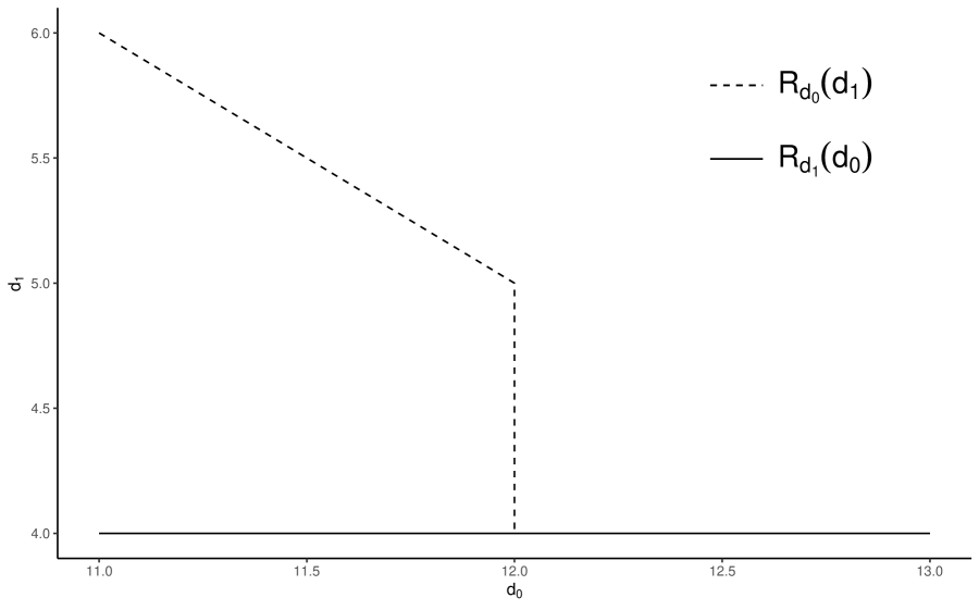
(a) $R_{d_{0}}(d_{1})$ and $R_{d_{1}}(d_{0})$

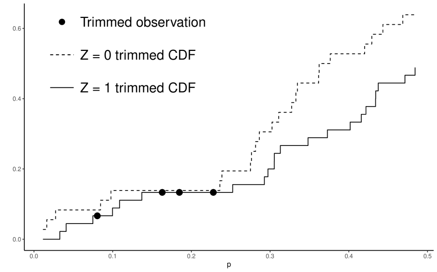
(b) $P^{-}$ region

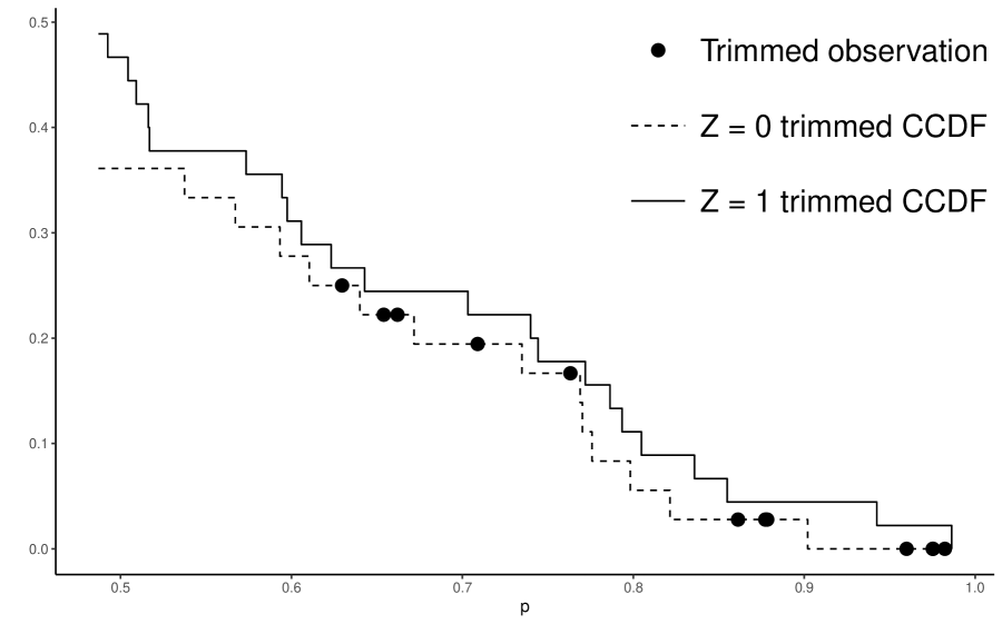
(c) $P^{+}$ region

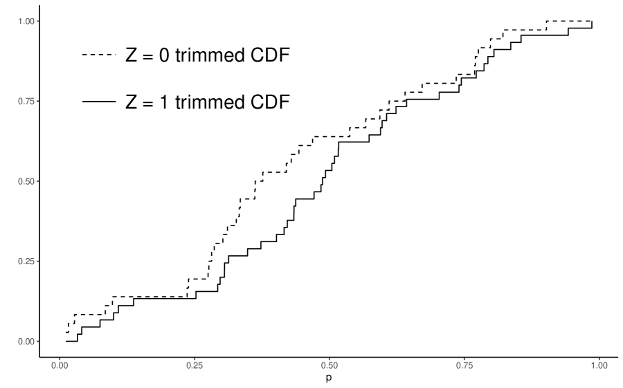
(d) Trimmed distributions

Figure 16: Example of the distillation algorithm. The sample consists of 100 observations. The data generating process sets $\Pr(Z=1)=1/2$ with propensity score uniformly distributed between 0 and 1 for $Z=0,1$. The interval $P^{-}$ includes all observations with a propensity weakly less than the median, while $P^{+}$ includes all observations with a propensity score above the median.

Appendix E Test Procedure for a Multi-valued Discrete Instrument

The test statistic and procedure of sections 3.1 and 3.1.1 can be extended to the case of a single multi-valued instrument. This test procedure forms pairs of neighbouring instrument values and jointly tests the nesting inequalities and index sufficiency for all pairs.

Let $Z\in\{z_{1},z_{2},...,z_{K}\}$, $n_{k}$ be the number of observations with $Z=z_{k}$, and $\lambda_{z_{k}}=\Pr(Z=z_{k})$. Form $K-1$ pairs of neighbouring instrument values $(z_{1},z_{2})$, $(z_{2},z_{3})$,…,$(z_{K-1},z_{L})$. For $k=1,...,K-1$, let $(S_{1k},S_{2k})$ be a pair of sample inclusion indicators corresponding to the subsample containing only observations with $Z\in\{z_{k},z_{k+1}\}$. $S_{1k}$ can be constructed by applying a distillation procedure to each $(z_{k},z_{k+1})$ subsample. The construction of $S_{2k}$ differs slightly from the headline test procedure in that it must now be based on the value of the two inverse probability weighting terms $\Pr(Z=z_{k}|p(X_{i},Z_{i}))$ and $\Pr(Z=z_{k+1}|p(X_{i},Z_{i}))$. For example $S_{2j}=1$ if $\Pr(Z=z_{k}|p(X_{i},Z_{i}))>0.05$ and $\Pr(Z=z_{k+1}|p(X_{i},Z_{i}))>0.05$.

For the subsample of observations with $Z\in\{z_{k},z_{k+1}\}$, denote the empirical conditional distributions of $(U,D,X)$ given $Z=z_{k+1}$ and $Z=z_{k}$ by $P_{n_{k+1}}$ and $Q_{n_{k}}$.

Define

$$f_{i}^{z_{k},S_{1k}}(A,d) =\frac{1\{U_{i}\in A,D_{i}=d\}S_{1ik}}{\Pr(S_{1k}=1|Z=z_{k})},$$

$$f_{i}^{z_{k+1},S_{1k}}(A,d) =\frac{1\{U_{i}\in A,D_{i}=d\}S_{1ik}}{\Pr(S_{1k}=1|Z=z_{k+1})},$$

$$g_{i}^{z_{k},S_{2k}}(A,d) =\frac{1\{U_{i}\in A,D_{i}=d\}\lambda_{z_{k}}S_{2ik}}{\Pr(Z=z_{k}|p(X_{i},Z_{i}))\Pr(S_{2k}=1|Z=z_{k})},$$

$$g_{i}^{z_{k+1},S_{2k}}(A,d) =\frac{1\{U_{i}\in A,D_{i}=d\}\lambda_{z_{k+1}}S_{2ik}}{\Pr(Z=z_{k}|p(X_{i},Z_{i}))\Pr(S_{2k}=1|Z=z_{k+1})}.$$

The test statistic is

$$T\equiv \underset{k\in\{1,...,K-1\}}{\max}T_{k}$$

$$T_{k}\equiv \max\left\{\sup_{A\in\mathcal{C}(\mathcal{Y}),d\in\{0,1\}}\frac{T_{1k}(A,d)}{\hat{\sigma}_{1k}(A,d)},\sup_{A\in\mathcal{C}(\mathcal{Y}),d\in\{0,1\}}\frac{T_{2k}(A,d)}{\hat{\sigma}_{2k}(A,d)},\sup_{A\in\mathcal{C}(\mathcal{Y}),d\in\{0,1\}}\frac{-T_{2k}(A,d)}{\hat{\sigma}_{2k}(A,d)}\right\},\ \text{where}$$

$$T_{1k}(A,d)= \sqrt{\frac{n_{k+1}n_{k}}{n_{k+1}+n_{k}}}\left[\left(Q_{n_{k}}f_{i}^{z_{k},S_{1k}}(A,1)-P_{n_{k+1}}f_{i}^{z_{k+1},S_{1k}}(A,1)\right)d\right.$$

$$+\left.(P_{n_{k+1}}f_{i}^{z_{k+1},S_{1k}}(A,0)-Q_{n_{k}}f_{i}^{z_{k},S_{1k}}(A,0))(1-d)\right]$$

$$T_{2k}(A,d)= \sqrt{\frac{n_{k+1}n_{k}}{n_{k+1}+n_{k}}}\left(Q_{n_{k}}g_{i}^{z_{k},S_{2k}}(A,d)-P_{n_{k+1}}g_{i}^{z_{k+1},S_{2k}}(A,d)\right)$$

$$\hat{\sigma}_{1k}^{2}(A,d)= \left\{\lambda_{z_{k}}[Q_{n_{k}}(f_{i}^{z_{k},S_{1k}}(A,1))^{2}-(Q_{n_{k}}f_{i}^{z_{k},S_{1k}}(A,1))^{2}]\right.$$

$$+\left.\lambda_{z_{k+1}}[P_{n_{k+1}}(f_{i}^{z_{k+1},S_{1k}}(A,1))^{2}-(P_{n_{k+1}}f_{i}^{z_{k+1},S_{1k}}(A,1))^{2}]\right\}d$$

$$+\left\{\lambda_{z_{k}}[Q_{n_{k}}(f_{i}^{z_{k},S_{1k}}(A,0))^{2}-(Q_{n_{k}}f_{i}^{z_{k},S_{1k}}(A,0))^{2}]\right.$$

$$+\left.\lambda_{z_{k+1}}[P_{n_{k+1}}(f_{i}^{z_{k+1},S_{1k}}(A,0))^{2}-(P_{n_{k+1}}f_{i}^{z_{k+1},S_{1k}}(A,0))^{2}]\right\}(1-d),$$

$$\hat{\sigma}_{2k}^{2}(A,d)= \lambda_{z_{k}}[Q_{n_{k}}(g_{i}^{z_{k},S_{2k}}(A,d))^{2}-(Q_{n_{0}}g_{i}^{z_{k}S_{2k}}(A,d))^{2}]+\lambda_{z_{k+1}}[P_{n_{k+1}}(g_{i}^{z_{k+1}S_{2k}}(A,d))^{2}-(P_{n_{k+1}}g_{i}^{z_{k+1}S_{2k}}(A,d))^{2}].$$

For the bootstrap, again let $(\hat{M}_{1},\dots,\hat{M}_{n})$ be iid random bootstrap multipliers such that they are independent of the original sample and satisfy $E(\hat{M}_{i})=0$ and $Var(\hat{M}_{i})=1$. A bootstrap analogue of $T$ can be constructed as

$$\hat{T}\equiv \underset{k\in\{1,...,K-1\}}{\max}\hat{T}_{k}$$

$$\hat{T}_{k}\equiv \max\left\{\sup_{A\in\mathcal{C}(\mathcal{Y}),d\in\{0,1\}}\frac{\hat{T}_{1k}(A,d)}{\sigma_{1k}(A,d)},\sup_{A\in\mathcal{C}(\mathcal{Y}),d\in\{0,1\}}\frac{\hat{T}_{2k}(A,d)}{\sigma_{2k}(A,d)},\sup_{A\in\mathcal{C}(\mathcal{Y}),d\in\{0,1\}}\frac{-\hat{T}_{2k}(A,d)}{\sigma_{2k}(A,d)}\right\},\ \text{where}$$

$$\hat{T}_{1k}(A,d)= \sqrt{\frac{n_{k+1}n_{k}}{n_{k+1}+n_{k}}}\left((\hat{Q}_{n_{k}}-Q_{n_{k}})f_{i}^{z_{k},S_{1k}}(A,1)-(\hat{P}_{n_{k+1}}-P_{n_{k+1}})f_{i}^{z_{k+1},S_{1k}}(A,1)\right)d$$

$$+\sqrt{\frac{n_{k+1}n_{k}}{n_{k+1}+n_{k}}}\left((\hat{P}_{n_{k+1}}-P_{n_{k+1}})f_{i}^{z_{k+1},S_{1k}}(A,0)-(\hat{Q}_{n_{k}}-Q_{n_{k}})f_{i}^{z_{k},S_{1k}}(A,0)\right)(1-d)$$

$$\hat{T}_{2k}(A,d)= \sqrt{\frac{n_{k+1}n_{k}}{n_{k+1}+n_{k}}}\left[(\hat{Q}_{n_{k}}-Q_{n_{k}})g_{i}^{z_{k},S_{2k}}(A,d)-(\hat{P}_{n_{k+1}}-P_{n_{k+1}})g_{i}^{z_{k+1},S_{2k}}(A,d)\right],$$

where, for the random variable $(a_{i}:i=1,\dots,n)$, we define

$$(\hat{Q}_{n_{k}}-Q_{n_{k}})a_{i} =\frac{1}{n_{k}}\sum_{i:Z_{i}=z_{k}}\hat{M}_{i}a_{i},\mspace{10.0mu}(\hat{P}_{n_{k+1}}-P_{n_{k+1}})a_{i}=\frac{1}{n_{k+1}}\sum_{i:Z_{i}=z_{k+1}}\hat{M}_{i}a_{i}.$$

Note that common bootstrap draws are used in constructing for all $\hat{T}_{k}$, rather than a separate draw being generated for each.

References

- Abadie (2003) Abadie, A. (2003): “Semiparametric instrumental variable estimation of treatment response models,” Journal of Econometrics, 113, 231–263.
- Acemoglu and Angrist (2000) Acemoglu, D. and J. Angrist (2000): “How Large Are Human-Capital Externalities? Evidence from Compulsory Schooling Laws,” NBER Macroeconomics Annual, 15, 9–59.
- Angrist et al. (2010) Angrist, J., V. Lavy, and A. Schlosser (2010): “Multiple Experiments for the Causal Link between the Quantity and Quality of Children,” Journal of Labor Economics, 28, 773–824.
- Angrist and Evans (1998) Angrist, J. D. and W. N. Evans (1998): “Children and Their Parents’ Labor Supply: Evidence from Exogenous Variation in Family Size,” The American Economic Review, 88, 450–477.
- Angrist and Imbens (1995) Angrist, J. D. and G. W. Imbens (1995): “Two-Stage Least Squares Estimation of Average Causal Effects in Models with Variable Treatment Intensity,” Journal of the American Statistical Association, 90, 431–442.
- Angrist et al. (1996) Angrist, J. D., G. W. Imbens, and D. B. Rubin (1996): “Identification of causal effects using instrumental variables,” Journal of the American statistical Association, 91, 444–455.
- Arai et al. (2022) Arai, Y., Y.-C. Hsu, T. Kitagawa, I. Mourifié, and Y. Wan (2022): “Testing identifying assumptions in fuzzy regression discontinuity designs,” Quantitative Economics, 13, 1–28.
- Balke and Pearl (1997) Balke, A. and J. Pearl (1997): “Bounds on treatment effects from studies with imperfect compliance,” Journal of the American Statistical Association, 92, 1171–1176.
- Becker et al. (2010) Becker, S. O., F. Cinnirella, and L. Woessmann (2010): “The trade-off between fertility and education: evidence from before the demographic transition,” Journal of Economic Growth, 15, 177–204.
- Bhuller et al. (2020) Bhuller, M., G. B. Dahl, K. V. Løken, and M. Mogstad (2020): “Incarceration, Recidivism, and Employment,” Journal of Political Economy, 128, 1269–1324.
- Black et al. (2010) Black, S. E., P. J. Devereux, and K. G. Salvanes (2010): “Small Family, Smart Family? Family Size and the IQ Scores of Young Men,” The Journal of Human Resources, 45, 33–58.
- Blandhol et al. (2022) Blandhol, C., J. Bonney, M. Mogstad, and A. Torgovitsky (2022): “When is TSLS Actually LATE?” arXiv.
- Bolzern and Huber (2017) Bolzern, B. and M. Huber (2017): “Testing the validity of the compulsory schooling law instrument,” Economics Letters, 159, 23–27.
- Brinch et al. (2017) Brinch, C. N., M. Mogstad, and M. Wiswall (2017): “Beyond LATE with a Discrete Instrument,” Journal of Political Economy, 125, 985–1039.
- Brunello et al. (2013) Brunello, G., M. Fort, G. Weber, and C. Weiss (2013): “Testing the internal validity of compulsory school reforms as instrument for years of schooling,” Working paper.
- Cameron and Taber (2004) Cameron, S. and C. Taber (2004): “Estimation of Educational Borrowing Constraints Using Returns to Schooling,” Journal of Political Economy, 112, 132–182.
- Card (1993) Card, D. (1993): “Using Geographic Variation in College Proximity to Estimate the Return to Schooling,” Working Paper 4483, National Bureau of Economic Research.
- Carneiro et al. (2011) Carneiro, P., J. J. Heckman, and E. J. Vytlacil (2011): “Estimating Marginal Returns to Education,” American Economic Review, 101, 2754–81.
- Chernozhukov et al. (2013) Chernozhukov, V., S. Lee, and A. M. Rosen (2013): “Intersection Bounds: Estimation and Inference,” Econometrica, 81, 667–737.
- Clark and Royer (2013) Clark, D. and H. Royer (2013): “The Effect of Education on Adult Mortality and Health: Evidence from Britain,” The American Economic Review, 103, 2087–2120.
- Conley and Glauber (2006) Conley, D. and R. Glauber (2006): “Parental Educational Investment and Children’s Academic Risk: Estimates of the Impact of Sibship Size and Birth Order from Exogenous Variation in Fertility,” The Journal of Human Resources, 41, 722–737.
- Cornelissen et al. (2018) Cornelissen, T., C. Dustmann, A. Raute, and U. Schönberg (2018): “Who Benefits from Universal Child Care? Estimating Marginal Returns to Early Child Care Attendance,” Journal of Political Economy, 126, 2356–2409.
- Coury et al. (2022) Coury, M., T. Kitagawa, A. Shertzer, and M. Turner (2022): “The Value of Piped Water and Sewers: Evidence from 19th Century Chicago,” Working Paper 29718, National Bureau of Economic Research.
- Cruces and Galiani (2007) Cruces, G. and S. Galiani (2007): “Fertility and female labor supply in Latin America: New causal evidence,” Labour Economics, 14, 565 – 573.
- Eisenhauer et al. (2015) Eisenhauer, P., J. J. Heckman, and E. Vytlacil (2015): “The Generalized Roy Model and the Cost-Benefit Analysis of Social Programs,” Journal of Political Economy, 123, 413–443.
- Farbmacher et al. (2022) Farbmacher, H., R. Guber, and S. Klaassen (2022): “Instrument Validity Tests With Causal Forests,” Journal of Business & Economic Statistics, 40, 605–614.
- Felfe and Lalive (2018) Felfe, C. and R. Lalive (2018): “Does early child care affect children’s development?” Journal of Public Economics, 159, 33 – 53.
- Frandsen et al. (2023) Frandsen, B., L. Lefgren, and E. Leslie (2023): “Judging Judge Fixed Effects,” American Economic Review, 113, 253–77.
- Heckman et al. (2018) Heckman, J. J., J. E. Humphries, and G. Veramendi (2018): “Returns to Education: The Causal Effects of Education on Earnings, Health, and Smoking,” Journal of Political Economy, 126, S197–S246.
- Heckman and Vytlacil (2005) Heckman, J. J. and E. Vytlacil (2005): “Structural equations, treatment effects, and econometric policy evaluation,” Econometrica, 73, 669–738.
- Heckman and Vytlacil (1999) Heckman, J. J. and E. J. Vytlacil (1999): “Local instrumental variables and latent variable models for identifying and bounding treatment effects,” Proceedings of the national Academy of Sciences, 96, 4730–4734.
- Heckman and Vytlacil (2001a) ——— (2001a): “Instrumental variables, selection models, and tight bounds on the average treatment effect,” in Econometric Evaluation of Labour Market Policies, Springer, 1–15.
- Heckman and Vytlacil (2001b) ——— (2001b): Local instrumental variables, Cambridge University Press, 1–46, International Symposia in Economic Theory and Econometrics.
- Huber (2015) Huber, M. (2015): “Testing the Validity of the Sibling Sex Ratio Instrument,” LABOUR, 29, 1–14.
- Huber and Mellace (2015) Huber, M. and G. Mellace (2015): “Testing instrument validity for LATE identification based on inequality moment constraints,” Review of Economics and Statistics, 97, 398–411.
- Imbens and Angrist (1994) Imbens, G. W. and J. D. Angrist (1994): “Identification and Estimation of Local Average Treatment Effects,” Econometrica: Journal of the Econometric Society, 467–475.
- Imbens and Rubin (1997) Imbens, G. W. and D. B. Rubin (1997): “Estimating outcome distributions for compliers in instrumental variables models,” The Review of Economic Studies, 64, 555–574.
- Kitagawa (2015) Kitagawa, T. (2015): “A Test for Instrument Validity,” Econometrica, 83, 2043–2063.
- Kline and Walters (2016) Kline, P. and C. R. Walters (2016): “Evaluating Public Programs with Close Substitutes: The Case of Head Start,” The Quarterly Journal of Economics, 131, 1795–1848.
- Kolesár (2013) Kolesár, M. (2013): “Estimation in an instrumental variables model with treatment effect heterogeneity,” unpublished manuscript.
- Kédagni and Mourifié (2020) Kédagni, D. and I. Mourifié (2020): “Generalized instrumental inequalities: testing the instrumental variable independence assumption,” Biometrika, 107, 661–675.
- Laffers and Mellace (2017) Laffers, L. and G. Mellace (2017): “A note on testing instrument validity for the identification of LATE.” Empirical Economics, 53, 1281 – 1286.
- Lleras-Muney (2005) Lleras-Muney, A. (2005): “The Relationship between Education and Adult Mortality in the United States,” The Review of Economic Studies, 72, 189–221.
- Lochner and Moretti (2004) Lochner, L. and E. Moretti (2004): “The Effect of Education on Crime: Evidence from Prison Inmates, Arrests, and Self-Reports,” American Economic Review, 94, 155–189.
- Machado et al. (2019) Machado, C., A. M. Shaikh, and E. J. Vytlacil (2019): “Instrumental variables and the sign of the average treatment effect,” Journal of Econometrics, 212, 522–555.
- Maestas et al. (2013) Maestas, N., K. J. Mullen, and A. Strand (2013): “Does Disability Insurance Receipt Discourage Work? Using Examiner Assignment to Estimate Causal Effects of SSDI Receipt,” American Economic Review, 103, 1797–1829.
- Mao and Sant’Anna (2020) Mao, M. and P. H. C. Sant’Anna (2020): “Testing instrument validity in marginal treatment effects models,” unpublished manuscript.
- Marshall (2016) Marshall, J. (2016): “Coarsening Bias: How Coarse Treatment Measurement Upwardly Biases Instrumental Variable Estimates,” Political Analysis, 24, 157–171.
- Mogstad et al. (2018) Mogstad, M., A. Santos, and A. Torgovitsky (2018): “Using instrumental variables for inference about policy relevant treatment parameters,” Econometrica, 86, 1589–1619.
- Mogstad and Torgovitsky (2018) Mogstad, M. and A. Torgovitsky (2018): “Identification and Extrapolation of Causal Effects with Instrumental Variables,” Annual Review of Economics, 10, 577–613.
- Mogstad et al. (2019) Mogstad, M., A. Torgovitsky, and C. R. Walters (2019): “The Causal Interpretation of Two-Stage Least Squares with Multiple Instrumental Variables,” Working Paper 25691, National Bureau of Economic Research.
- Mogstad et al. (2020) ——— (2020): “Policy Evaluation with Multiple Instrumental Variables,” Working Paper 27546, National Bureau of Economic Research.
- Mourifié and Wan (2017) Mourifié, I. and Y. Wan (2017): “Testing local average treatment effect assumptions,” Review of Economics and Statistics, 99, 305–313.
- Oreopoulos (2006) Oreopoulos, P. (2006): “Estimating Average and Local Average Treatment Effects of Education when Compulsory Schooling Laws Really Matter,” American Economic Review, 96, 152–175.
- Rosenzweig and Wolpin (2000) Rosenzweig, M. R. and K. I. Wolpin (2000): “Natural ”Natural Experiments” in Economics,” Journal of Economic Literature, 38, 827–874.
- Stephens and Yang (2014) Stephens, Melvin, J. and D.-Y. Yang (2014): “Compulsory Education and the Benefits of Schooling,” American Economic Review, 104, 1777–92.
- Sun (2021) Sun, Z. (2021): “Instrument Validity for Heterogeneous Causal Effects,” .
- Słoczyński (2021) Słoczyński, T. (2021): “When Should We (Not) Interpret Linear IV Estimands as LATE?” .
- Van Der Vaart and Wellner (1996) Van Der Vaart, A. W. and J. Wellner (1996): Weak convergence and empirical processes: with applications to statistics, Springer Science & Business Media.