On the application of the SCD semismooth* Newton method
to variational inequalities of the second kind

Abstract. The paper starts with a description of the SCD (subspace containing derivative) mappings and the SCD semismooth^∗ Newton method for the solution of general inclusions. This method is then applied to a class of variational inequalities of the second kind. As a result, one obtains an implementable algorithm exhibiting a locally superlinear convergence. Thereafter we suggest several globally convergent hybrid algorithms in which one combines the SCD semismooth^∗ Newton method with selected splitting algorithms for the solution of monotone variational inequalities. Finally we demonstrate the efficiency of one of these methods via a Cournot-Nash equilibrium, modeled as a variational inequalities of the second kind, where one admits really large numbers of players (firms) and produced commodities.
Key words. Newton method, semismoothness^∗, superlinear convergence, global convergence, generalized equation, coderivatives.
AMS Subject classification. 65K10, 65K15, 90C33.

1 Introduction

In [3] the authors proposed the so-called semismooth* Newton method for the numerical solution of a general inclusion

$$0\in H(x),$$

where $H:\mathbb{R}^{n}\rightrightarrows\mathbb{R^{n}}$ is a closed-graph multifunction. This method has been further developed in [4], where it has coined the name SCD (subspace containing derivative) semismooth* Newton method. When compared with the original method from [4], the new variant requires a slightly stronger approximation of the limiting coderivative of $H$, but exhibits locally superlinear convergence under substantially less restrictive assumptions. The aim of this paper is to work out this Newton-type method for the numerical solution of the generalized equation (GE)

$$0\in H(x):=f(x)+\partial q(x),$$ (1.1)

where $f:\mathbb{R}^{n}\rightarrow\mathbb{R}^{n}$ is continuously differentiable, $q:\mathbb{R}^{n}\rightarrow\overline{\mathbb{R}}$ is proper convex and lower-semicontinuous (lsc) and $\partial$ stands for the classical Moreau-Rockafellar subdifferential. It is easy to see that GE (1.1) is equivalent to the variational inequality (VI):

Find $\bar{x}\in\mathbb{R}^{n}$ such that

$$\langle f(\bar{x}),x-\bar{x}\rangle+q(x)-q(\bar{x})\geq 0~{}\mbox{ for all }~{}x\in\mathbb{R}^{n}.$$ (1.2)

The model (1.2) has been introduced in [6] and one speaks about the variational inequality (VI) of the second kind. It is widely used in the literature dealing with equilibrium models in continuum mechanics cf., e.g., [8] and the references therein. For the numerical solution of GE (1.1), a number of methods can be used ranging from nonsmooth optimization methods (applicable when $\nabla f$ is symmetric) up to a broad family of splitting methods (usable when $H$ is monotone), cf. [1, Chapter 12]. If GE (1.1) amounts to stationarity condition for a Nash game, then also a simple coordinate-wise optimization technique can be used, cf. [11] and [14]. Concerning the Newton type methods, let us mention, for instance, the possibility to write down GE (1.1) as an equation on a monotone graph, which enables us to apply the Newton procedure from [16]. Note, however, that the subproblems to be solved in this approach are typically rather difficult. In other papers the authors reformulate the problem as a (standard) nonsmooth equation which is then solved by the classical semismooth Newton method, see, e.g., [9, 20].

As mentioned above, in this paper we will investigate the numerical solution of GE (1.1) via the SCD semismooth* Newton method developed in [4]. In contrast to the Newton methods by Josephy, in this method (as well as in its original variant from [3]) the multi-valued part of (1.1) is also approximated and, differently to some other Newton-type methods, this approximation is provided by means of a linear subspace belonging to the graph of the limiting coderivative of $\partial q$. In this way the computation of the Newton direction reduces to the solution of a linear system of equations. To ensure locally superlinear convergence, two properties have to be fulfilled. The first one is a weakening of the semismooth^∗ property from [3] and pertains the subdifferential mapping $\partial q$. The second one, called SCD regularity, concerns the mapping $H$ and amounts, roughly speaking, to the strong metric subregularity of the considered GE around the solution.

The plan of the paper is as follows. After the preliminary Section 2, where we provide the needed background from modern variational analysis, Section 3 is devoted to the broad class of SCD mappings, which is the basic framework for the application of the used method. In particular, the subdifferential of a proper convex lsc function is an SCD mapping. In Section 4 the SCD semismooth* Newton method is described and its convergence is analyzed. Thereafter, in Section 5 we develop an implementable version of the method for the solution of GE (1.1) and show its locally superlinear convergence under mild assumptions. Section 6 deals with the issue of global convergence. First we suggest a heuristic modification of the method from the preceding section which exhibits very good convergence properties in the numerical experiments. Thereafter we show global convergence for a family of hybrid algorithms, where one combines the semismooth* Newton method with various frequently used splitting methods. Finally, in Section 7 we demonstrate the efficiency of the developed methods via a Cournot-Nash equilibrium problem taken over from [13] which can be modeled in the form of GE (1.1). In contrast to the numerical approach in [13], we may work here with ”arbitrarily” large numbers of player (firms) and commodities,

The following notation is employed. Given a matrix $A$, ${\rm rge\;}A$ and ${\rm ker\;}A$ denote the range space and the kernel of $A$, respectively, and $\|A\|$ stands for its spectral norm. For a set $\Omega$, ${\rm dist}(x,\Omega):=\inf_{a\in\Omega}\|x-a\|$ signifies the distance from $x$ to $\Omega$ and ${\rm ri\,}\Omega$ is the relative interior of $\Omega$. Further, $L^{\perp}$ denotes the anihilator of a linear subspace $L$ and ${\rm diag\,}(A,B)$ means a block diagonal matrix with matrices $A,B$ as diagonal blocks.

2 Preliminaries

Throughout the whole paper, we will frequently use the following basic notions of modern variational analysis.

Definition 2.1.

Let $A$ be a set in $\mathbb{R}^{s}$, $\bar{x}\in A$ and $A$ be locally closed around $\bar{x}$. Then

1. The tangent (contingent, Bouligand) cone to $A$ at $\bar{x}$ is given by

   $$T_{A}(\bar{x}):=\mathop{{\rm Lim}\,{\rm sup}}\limits_{t\downarrow 0}\frac{A-\bar{x}}{t}.$$

2. The set

   $$\widehat{N}_{A}(\bar{x}):=(T_{A}(\bar{x}))^{\circ}$$

   is the regular (Fréchet) normal cone to $A$ at $\bar{x}$, and

   $$N_{A}(\bar{x}):=\mathop{{\rm Lim}\,{\rm sup}}\limits_{\stackrel{{\scriptstyle A}}{{x\rightarrow\bar{x}}}}\widehat{N}_{A}(x)$$

   is the limiting (Mordukhovich) normal cone to $A$ at $\bar{x}$.

In this definition ”$\mathop{{\rm Lim}\,{\rm sup}}$” stands for the Painlevé-Kuratowski outer (upper) set limit, see, e.g., [18]. The above listed cones enable us to describe the local behavior of set-valued maps via various generalized derivatives. Let $F:\mathbb{R}^{n}\rightrightarrows\mathbb{R}^{m}$ be a (set-valued) mapping with the domain and the graph

$$\mathrm{dom}\,F:=\{x\in\mathbb{R}^{n}\,\mid\,F(x)\not=\emptyset\},\quad\mathrm{gph}\,F:=\{(x,y)\in\mathbb{R}^{n}\times\mathbb{R}^{m}\,\mid\,y\in F(x)\}.$$

Definition 2.2.

Consider a (set-valued) mapping $F:\mathbb{R}^{n}\rightrightarrows\mathbb{R}^{m}$ and let $\mathrm{gph}\,F$ be locally closed around some $(\bar{x},\bar{y})\in\mathrm{gph}\,F$.

1. The multifunction $DF(\bar{x},\bar{y}):\mathbb{R}^{n}\rightrightarrows\mathbb{R}^{m}$, given by $\mathrm{gph}\,DF(\bar{x},\bar{y})=T_{\mathrm{gph}\,F}(\bar{x},\bar{y})$, is called the graphical derivative of $F$ at $(\bar{x},\bar{y})$.

2. The multifunction $D^{\ast}F(\bar{x},\bar{y}):\mathbb{R}^{m}\rightrightarrows\mathbb{R}^{n}$, defined by

   $$\mathrm{gph}\,D^{\ast}F(\bar{x},\bar{y})=\{(y^{*},x^{*})\,\mid\,(x^{*},-y^{*})\in N_{\mathrm{gph}\,F}(\bar{x},\bar{y})\}$$

   is called the limiting (Mordukhovich) coderivative of $F$ at $(\bar{x},\bar{y})$.

Let us now recall the following regularity notions.

Definition 2.3.

Let $F:\mathbb{R}^{n}\rightrightarrows\mathbb{R}^{m}$ be a a (set-valued) mapping and let $(\bar{x},\bar{y})\in\mathrm{gph}\,F$.

1. $F$ is said to be metrically subregular at $(\bar{x},\bar{y})$ if there exists $\kappa\geq 0$ along with some neighborhood $X$ of $\bar{x}$ such that

   $${\rm dist}(x,F^{-1}(\bar{y}))\leq\kappa\,{\rm dist}(\bar{y},F(x))\ \forall x\in X.$$

2. $F$ is said to be strongly metrically subregular at $(\bar{x},\bar{y})$ if it is metrically subregular at $(\bar{x},\bar{y})$ and there exists a neighborhood $X^{\prime}$ of $\bar{x}$ such that $F^{-1}(\bar{y})\cap X^{\prime}=\{\bar{x}\}$.

3. $F$ is said to be metrically regular around $(\bar{x},\bar{y})$ if there is $\kappa\geq 0$ together with neighborhoods $X$ of $\bar{x}$ and $Y$ of $\bar{y}$ such that

   $${\rm dist}(x,F^{-1}(y))\leq\kappa\,{\rm dist}(y,F(x))\ \forall(x,y)\in X\times Y.$$

4. $F$ is said to be strongly metrically regular around $(\bar{x},\bar{y})$ if it is metrically regular around $(\bar{x},\bar{y})$ and $F^{-1}$ has a single-valued localization around $(\bar{y},\bar{y})$, i.e., there are open neighborhoods $Y^{\prime}$ of $\bar{y}$, $X^{\prime}$ of $\bar{x}$ and a mapping $h:Y^{\prime}\to\mathbb{R}^{n}$ with $h(\bar{y})=\bar{x}$ such that $\mathrm{gph}\,F\cap(X^{\prime}\times Y^{\prime})=\{(h(y),y)\,\mid\,y\in Y^{\prime}\}$.

It is easy to see that the strong metric regularity around $(\bar{x},\bar{y})$ implies the strong metric subregularity at $(\bar{x},\bar{y})$ and the metric regularity around $(\bar{x},\bar{y})$ implies the metric subregularity at $(\bar{x},\bar{y})$. To check the metric regularity one often employs the so-called Mordukhovich criterion, according to which this property around $(\bar{x},\bar{y})$ is equivalent with the condition

$$0\in D^{*}F(\bar{x},\bar{y})(y^{*})\ \Rightarrow\ y^{*}=0.$$ (2.3)

For pointwise characterizations of the other stability properties from Definition 2.3 the reader is referred to [4, Theorem 2.7].

We end up this preparatory section with a definition of the semismooth^∗ property which paved the way both to semismooth^∗ Newton method in [3] as well as to the SCD semismooth^∗ Newton method in [4].

Definition 2.4.

We say that $F:\mathbb{R}^{n}\rightrightarrows\mathbb{R}^{n}$ is semismooth^∗ at $(\bar{x},\bar{y})\in\mathrm{gph}\,F$ if for every $\epsilon>0$ there is some $\delta>0$ such that the inequality

$$|\langle x^{*},x-\bar{x}\rangle-\langle y^{*},y-\bar{y}\rangle| \leq\epsilon\|(x,y)-(\bar{x},\bar{y})\|\|(x^{*},y^{*})\|$$

holds for all $(x,y)\in\mathrm{gph}\,F\cap{\cal B}_{\delta}(\bar{x},\bar{y})$ and all $(y^{*},x^{*})$ belonging to $\mathrm{gph}\,D^{\ast}F(\bar{x},\bar{y})$.

3 On SCD mappings

3.1 Basic properties

In this section we want to recall the basic definitions and features of the SCD property introduced in the recent paper [4].

In what follows we denote by ${\cal Z}_{n}$ the metric space of all $n$-dimensional subspaces of $\mathbb{R}^{2n}$ equipped with the metric

$$d_{\cal Z}(L_{1},L_{2}):=\|P_{L_{1}}-P_{L_{2}}\|$$

where $P_{L_{i}}$ is the symmetric $2n\times 2n$ matrix representing the orthogonal projection on $L_{i}$, $i=1,2$.

Sometimes we will also work with bases for the subspaces $L\in{\cal Z}_{n}$. Let ${\cal M}_{n}$ denote the collection of all $2n\times n$ matrices with full column rank $n$ and for $L\in{\cal Z}_{n}$ we define

$${\cal M}(L):=\{Z\in{\cal M}_{n}\,\mid\,{\rm rge\;}Z=L\},$$

i.e., the columns of $Z\in{\cal M}(L)$ are a basis for $L$.

We treat every element of $\mathbb{R}^{2n}$ as a column vector. In order to keep notation simple we write $(u,v)$ instead of $\begin{pmatrix}u\\ v\end{pmatrix}\in\mathbb{R}^{2n}$ when this does not lead to confusion. In order to refer to the components of the vector $z=\begin{pmatrix}u\\ v\end{pmatrix}$ we set $\pi_{1}(z):=u,\ \pi_{2}(z)=v$.

Let $L\in{\cal Z}_{n}$ and consider $Z\in{\cal M}(L)$. Then we can partition $Z$ into two $n\times n$ matrices $A$ and $B$ and we will write $Z=(A,B)$ instead of $Z=\begin{pmatrix}A\\ B\end{pmatrix}$. It follows that ${\rm rge\;}(A,B):=\{(Au,Bu)\,\mid\,u\in\mathbb{R}^{n}\}\doteq\{\begin{pmatrix}Au\\ Bu\end{pmatrix}\,\mid\,u\in\mathbb{R}^{n}\}=L$. Similarly as before, we will also use $\pi_{1}(Z):=A$, $\pi_{2}(Z):=B$ for referring to the two $n\times n$ parts of $Z$.

Further, for every $L\in{\cal Z}_{n}$ we can define

$$L^{*} :=\{(-v^{*},u^{*})\,\mid\,(u^{*},v^{*})\in L^{\perp}\},$$

where $L^{\perp}$ denotes as usual the orthogonal complement of $L$. Then it can be shown that $(L^{*})^{*}=L$ and $d_{\cal Z}(L_{1},L_{2})=d_{\cal Z}(L_{1}^{*},L_{2}^{*})$. Thus the mapping $L\to L^{*}$ defines an isometry on ${\cal Z}_{n}$.

We denote by $S_{n}$ the $2n\times 2n$ orthogonal matrix

$$S_{n}:=\begin{pmatrix}0&-I\\ I&0\end{pmatrix}$$

so that $L^{*}=S_{n}L^{\perp}$.

Definition 3.1.

Consider a mapping $F:R^{n}\rightrightarrows\mathbb{R}^{n}$.

1. We call $F$ graphically smooth of dimension $n$ at $(x,y)\in\mathrm{gph}\,F$, if $T_{\mathrm{gph}\,F}(x,y)=\mathrm{gph}\,DF(x,y)\in{\cal Z}_{n}$. Further we denote by ${\cal O}_{F}$ the set of all points where $F$ is graphically smooth of dimension $n$.

2. We associate with $F$ the four mappings $\widehat{\mathcal{S}}F:\mathrm{gph}\,F\rightrightarrows{\cal Z}_{n}$, $\widehat{\mathcal{S}}^{*}F:\mathrm{gph}\,F\rightrightarrows{\cal Z}_{n}$, ${\mathcal{S}}F:\mathrm{gph}\,F\rightrightarrows{\cal Z}_{n}$, ${\mathcal{S}}^{*}F:\mathrm{gph}\,F\rightrightarrows{\cal Z}_{n}$, given by

   $$\widehat{\mathcal{S}}F(x,y) :=\begin{cases}\{\mathrm{gph}\,DF(x,y)\}&\mbox{if $(x,y)\in{\cal O}_{F}$,}\\ \emptyset&\mbox{else,}\end{cases}$$

   $$\widehat{\mathcal{S}}^{*}F(x,y) :=\begin{cases}\{\mathrm{gph}\,DF(x,y)^{*}\}&\mbox{if $(x,y)\in{\cal O}_{F}$,}\\ \emptyset&\mbox{else,}\end{cases}$$

   $${\mathcal{S}}F(x,y) :=\mathop{{\rm Lim}\,{\rm sup}}_{(u,v)\mathop{\longrightarrow}\limits^{{\mathrm{gph}\,F}}(x,y)}\widehat{\mathcal{S}}F(u,v)$$

   $$=\{L\in{\cal Z}_{n}\,\mid\,\exists(x_{k},y_{k})\mathop{\longrightarrow}\limits^{{{\cal O}_{F}}}(x,y):\ \lim_{k\to\infty}d_{\cal Z}(L,\mathrm{gph}\,DF(x_{k},y_{k}))=0\},$$

   $${\mathcal{S}}^{*}F(x,y) :=\mathop{{\rm Lim}\,{\rm sup}}_{(u,v)\mathop{\longrightarrow}\limits^{{\mathrm{gph}\,F}}(x,y)}\widehat{\mathcal{S}}^{*}F(u,v)$$

   $$=\{L\in{\cal Z}_{n}\,\mid\,\exists(x_{k},y_{k})\mathop{\longrightarrow}\limits^{{{\cal O}_{F}}}(x,y):\ \lim_{k\to\infty}d_{\cal Z}(L,\mathrm{gph}\,DF(x_{k},y_{k})^{*})=0\}.$$

3. We say that $F$ has the SCD (subspace containing derivative) property at $(x,y)\in\mathrm{gph}\,F$, if ${\mathcal{S}}^{*}F(x,y)\not=\emptyset$. We say that $F$ has the SCD property around $(x,y)\in\mathrm{gph}\,F$, if there is a neighborhood $W$ of $(x,y)$ such that $F$ has the SCD property at every $(x^{\prime},y^{\prime})\in\mathrm{gph}\,F\cap W$. Finally, we call $F$ an SCD mapping if $F$ has the SCD property at every point of its graph.

Since $L\to L^{*}$ is an isometry on ${\cal Z}_{n}$ and $(L^{*})^{*}=L$, the mappings ${\mathcal{S}}^{*}F$ and ${\mathcal{S}}F$ are related via

$${\mathcal{S}}^{*}F(x,y)=\{L^{*}\,\mid\,L\in{\mathcal{S}}F(x,y)\},\ {\mathcal{S}}F(x,y)=\{L^{*}\,\mid\,L\in{\mathcal{S}}^{*}F(x,y)\}.$$

The name SCD property is motivated by the following statement.

Lemma 3.2 (cf.[4, Lemma 3.7]).

Let $F:\mathbb{R}^{n}\rightrightarrows\mathbb{R}^{n}$ and let $(x,y)\in\mathrm{gph}\,F$. Then $L\subseteq\mathrm{gph}\,D^{*}F(x,y)$ $\forall L\in{\mathcal{S}}^{*}F(x,y)$.

Next we turn to the notion of SCD regularity.

Definition 3.3.

1. We denote by ${\cal Z}_{n}^{\rm reg}$ the collection of all subspaces $L\in{\cal Z}_{n}$ such that

   $$(y^{*},0)\in L\ \Rightarrow\ y^{*}=0.$$

2. A mapping $F:\mathbb{R}^{n}\rightrightarrows\mathbb{R}^{n}$ is called SCD regular around $(x,y)\in\mathrm{gph}\,F$, if $F$ has the SCD property around $(x,y)$ and

   $$(y^{*},0)\in L\Rightarrow\ y^{*}=0\ \forall L\in{\mathcal{S}}^{*}F(x,y),$$ (3.4)

   i.e., $L\in{\cal Z}_{n}^{\rm reg}$ for all $L\in{\mathcal{S}}^{*}F(x,y)$. Further, we will denote by

   $${\rm scd\,reg\;}F(x,y):=\sup\{\|y^{*}\|\,\mid\,(y^{*},x^{*})\in L,L\in{\mathcal{S}}^{*}F(x,y),\|x^{*}\|\leq 1\}$$

   the modulus of SCD regularity of $F$ around $(x,y)$.

Since the elements of ${\mathcal{S}}^{*}F(x,y)$ are contained in $\mathrm{gph}\,D^{*}F(x,y)$, it follows from the Mordukhovich criterion (2.3) that SCD regularity is weaker than metric regularity.

In the following propostion we state some basic properties of subspaces $L\in{\cal Z}_{n}^{\rm reg}$.

Proposition 3.4 (cf.[4, Proposition 4.2]).

Given a $2n\times n$ matrix $Z$, there holds ${\rm rge\;}Z\in{\cal Z}_{n}^{\rm reg}$ if and only if the $n\times n$ matrix $\pi_{2}(Z)$ is nonsingular. Thus, for every $L\in{\cal Z}_{n}^{\rm reg}$ there is a unique $n\times n$ matrix $C_{L}$ such that $L={\rm rge\;}(C_{L},I)$. Further, $L^{*}={\rm rge\;}(C_{L}^{T},I)\in{\cal Z}_{n}^{\rm reg}$,

$$\langle x^{*},C_{L}^{T}v\rangle=\langle y^{*},v\rangle\ \forall(y^{*},x^{*})\in L\forall v\in\mathbb{R}^{n}.$$

and

$$\|y^{*}\|\leq\|C_{L}\|\|x^{*}\|\ \forall(y^{*},x^{*})\in L.$$

Note that for every $L\in{\cal Z}_{n}^{{\rm reg\,}}$ and every $(A,B)\in{\cal M}(L)$ the matrix $B$ is nonsingular and $C_{L}=AB^{-1}$.

Combining [4, Equation (34), Lemma 4.7, Proposition 4.8] we obtain the following lemma

Lemma 3.5.

Assume that $F:\mathbb{R}^{n}\rightrightarrows\mathbb{R}^{n}$ is SCD regular around $(\bar{x},\bar{y})\in\mathrm{gph}\,F$. Then

$${\rm scd\,reg\;}F(\bar{x},\bar{y})=\sup\{\|C_{L}\|\,\mid\,L\in{\mathcal{S}}^{*}F(\bar{x},\bar{y})\}<\infty$$

Moreover, $F$ is SCD regular around every $(x,y)\in\mathrm{gph}\,F$ sufficiently close to $(\bar{x},\bar{y})$ and

$$\limsup_{(x,y)\mathop{\longrightarrow}\limits^{\mathrm{gph}\,F}(\bar{x},\bar{y})}{\rm scd\,reg\;}F(x,y)\leq{\rm scd\,reg\;}F(\bar{x},\bar{y}).$$

3.2 On the SCD property of the subdifferential of convex functions

Theorem 3.6 (cf.[4, Corollary 3.28]).

For every proper lsc convex function $q:\mathbb{R}^{n}\to\bar{\mathbb{R}}$ the subdifferential mapping $\partial q$ is an SCD mapping and for every $(x,x^{*})\in\mathrm{gph}\,\partial q$ and for every $L\in{\mathcal{S}}^{*}\partial q(x,x^{*})={\mathcal{S}}\partial q(x,x^{*})$ there is a symmetric positive semidefinite $n\times n$ matrix $B$ with $\|B\|\leq 1$ such that $L={\rm rge\;}(B,I-B)=L^{*}$.

The representation of $L$ via the matrix $B$ is only one possibility. E.g., if $q$ is twice continuously differentiable then ${\rm rge\;}(I,\nabla^{2}q(x))=\mathrm{gph}\,D^{*}\partial q(x,\nabla q(x))$ and the relation between $B$ and $\nabla^{2}q(x)$ is given by $B=(I+\nabla^{2}q(x))^{-1}$, $I-B=(I+\nabla^{2}q(x))^{-1}\nabla^{2}q(x)$ and $\nabla^{2}q(x)=B^{-1}(I-B)$.

Example 3.7.

Assume that $q(x)=\|x\|$ so that

$$\partial q(x)=\begin{cases}{\cal B}&\mbox{for $x=0$}\\ \frac{x}{\|x\|}&\mbox{otherwise.}\end{cases}$$

By virtue of Theorem 3.6, $\partial q$ is an SCD mapping. When considering a pair $(\bar{x},{\bar{x}^{\ast}})\in\mathrm{gph}\,\partial q$ with $\bar{x}=0$ and $\|{\bar{x}^{\ast}}\|<1$, then it is easy to see that $\partial q$ is graphically smooth of dimension $n$ at $(\bar{x},{\bar{x}^{\ast}})$ and, by Definition 3.1,

$${\mathcal{S}}\partial q(\bar{x},{\bar{x}^{\ast}})={\mathcal{S}}^{*}\partial q(\bar{x},{\bar{x}^{\ast}})=\big{\{}\{0\}\times\mathbb{R}^{n}\big{\}}.$$

In this case we have the representation $\{0\}\times\mathbb{R}^{n}={\rm rge\;}(B,I-B)$ with $B=0$. If $x\not=0$ then $q$ is even twice continuously differentiable near $x$ and, as pointed out below Theorem 3.6, with ${\bar{x}^{\ast}}=\frac{x}{\|x\|}$ one has

$${\mathcal{S}}\partial q(\bar{x},{\bar{x}^{\ast}})={\mathcal{S}}^{*}\partial q(\bar{x},{\bar{x}^{\ast}})={\rm rge\;}(B_{x},I-B_{x})={\rm rge\;}(I,\nabla^{2}q(x))$$

with

$$B_{x}=\big{(}I+\nabla^{2}q(x)\big{)}^{-1}=\left(I+\frac{1}{\|x\|}\Big{(}I-\frac{xx^{T}}{\|x\|^{2}}\Big{)}\right)^{-1}=\left(\frac{\|x\|+1}{\|x\|}\Big{(}I-\frac{xx^{T}}{\|x\|^{2}(1+\|x\|)}\Big{)}\right)^{-1}.$$

We claim that

$$B_{x}=\frac{\|x\|}{\|x\|+1}\Big{(}I+\frac{xx^{T}}{\|x\|^{3}}\Big{)}.$$ (3.5)

Indeed,

$$\Big{(}I-\frac{xx^{T}}{\|x\|^{2}(1+\|x\|)}\Big{)}\Big{(}I+\frac{xx^{T}}{\|x\|^{3}}\Big{)} =I+xx^{T}\Big{(}\frac{1}{\|x\|^{3}}-\frac{1}{\|x\|^{2}(1+\|x\|)}-\frac{\|x\|^{2}}{\|x^{5}\|(1+\|x\|)}\Big{)}$$

$$=I+xx^{T}\Big{(}\frac{1+\|x\|-\|x\|-1}{\|x\|^{3}(1+\|x\|)}\Big{)}=I,$$

and so formula (3.5) holds true.

Finally consider the point $(\bar{x},{\bar{x}^{\ast}})$ with $\bar{x}=0$ and $\|{\bar{x}^{\ast}}\|=1$. By Definition 3.1 and Theorem 3.6 one has that

$${\mathcal{S}}\partial q(\bar{x},{\bar{x}^{\ast}})={\mathcal{S}}^{*}\partial q(\bar{x},{\bar{x}^{\ast}})=\big{\{}\{0\}\times\mathbb{R}^{n}\big{\}}\;\cup\;\mathop{{\rm Lim}\,{\rm sup}}_{{\textstyle{x\to 0,x\not=0\atop\frac{x}{\|x\|}\to{\bar{x}^{\ast}}}}}\;{\rm rge\;}(B_{x},I-B_{x}).$$

Since the matrices $B_{x}$ are bounded, the above $\mathop{{\rm Lim}\,{\rm sup}}$ amounts to ${\rm rge\;}(B,I-B)$ where, taking into account (3.5),

$$B=\lim_{{\textstyle{x\to 0,x\not=0\atop\frac{x}{\|x\|}\to{\bar{x}^{\ast}}}}}B_{x}={\bar{x}^{\ast}}{\bar{x}^{\ast}}{}^{T}$$

However, note that

$$\lim_{{\textstyle{x\to 0,x\not=0\atop\frac{x}{\|x\|}\to{\bar{x}^{\ast}}}}}\nabla^{2}q(x)$$

does not exist. Finally note that, at points $(\bar{x},{\bar{x}^{\ast}})$ with $\bar{x}=0$ and $\|{\bar{x}^{\ast}}\|=1$, one has

$$\mathrm{gph}\,D^{*}\partial q(\bar{x},{\bar{x}^{\ast}})={\mathcal{S}}^{*}\partial q(\bar{x},{\bar{x}^{\ast}})\cup\{(s,s^{*})\,\mid\,s\in\mathbb{R}_{-}\{{\bar{x}^{\ast}}\},\langle s^{*},{\bar{x}^{\ast}}\rangle\leq 0\},$$

where the last term is generated by sequences $(0,x^{*})\to(0,{\bar{x}^{\ast}})$ with $\|x^{*}\|=1$. Thus, in this situation the mapping ${\mathcal{S}}^{*}\partial q(\bar{x},{\bar{x}^{\ast}})$ has a simpler structure than the limiting coderivative $D^{*}\partial q(\bar{x},{\bar{x}^{\ast}})$ (similarly as in [4, Example 3.29].)

In our numerical experiments we will use convex functions with some separable structure, which carries over to ${\mathcal{S}}^{*}\partial q$.

Lemma 3.8.

If $q(x_{1},x_{2})=q(x_{1})+q_{2}(x_{2})$ for lsc convex functions $q_{i}:\mathbb{R}^{n_{i}}\to\bar{\mathbb{R}}$, $i=1,2$, then for every $((\bar{x}_{1},\bar{x}_{2}),(\bar{x}_{1}^{*},\bar{x}_{2}^{*}))\in\mathrm{gph}\,\partial q$ there holds

$${\mathcal{S}}\partial q((\bar{x}_{1},\bar{x}_{2}),(\bar{x}_{1}^{*},\bar{x}_{2}^{*}))=\Big{\{}\{((u_{1},u_{2}),(u_{1}^{*},u_{2}^{*}))\,\mid\,(u_{i},u_{i}^{*})\in L_{i},i=1,2\}\,\mid\,L_{i}\in{\mathcal{S}}\partial q_{i}(\bar{x}_{i},\bar{x}_{i}^{*}),\ i=1,2\Big{\}}.$$

Proof.

We claim that ${\cal O}_{\partial q}=\{((x_{1},x_{2}),(x_{1}^{*},x_{2}^{*}))\,\mid\,(x_{i},x_{i}^{*})\in{\cal O}_{\partial q_{i}},\ i=1,2\}$ and that

$$T_{\mathrm{gph}\,\partial q}((x_{1},x_{2}),(x_{1}^{*},x_{2}^{*}))=\{((u_{1},u_{2}),(u_{1}^{*},u_{2}^{*}))\,\mid\,(u_{i},u_{i}^{*})\in T_{\mathrm{gph}\,\partial q_{i}}(x_{i},x_{i}^{*}),\ i=1,2\}$$ (3.6)

holds for all $((x_{1},x_{2}),(x_{1}^{*},x_{2}^{*}))\in{\cal O}_{\partial q}$. Indeed, if $((x_{1},x_{2}),(x_{1}^{*},x_{2}^{*}))\in{\cal O}_{\partial q}$ then $(x_{1},x_{1}^{*})\in{\cal O}_{\partial q_{1}}$ because of $\{((u_{1},0),(u_{1}^{*},0))\,\mid\,(u_{1},u_{1}^{*})\in\partial q_{1}(x_{1},x_{1}^{*})\}\subseteq T_{\mathrm{gph}\,\partial q}((x_{1},x_{2}),(x_{1}^{*},x_{2}^{*}))$ and, analogously, $(x_{2},x_{2}^{*})\in{\cal O}_{\partial q_{1}}$. This proves ${\cal O}_{\partial q}\subseteq\{((x_{1},x_{2}),(x_{1}^{*},x_{2}^{*}))\,\mid\,(x_{i},x_{i}^{*})\in{\cal O}_{\partial q_{i}},\ i=1,2\}$. To show the reverse inclusion, consider $(x_{i},x_{i}^{*})\in{\cal O}_{q_{i}}$, $i=1,2$. Taking into account [4, Corollary 3.28, Remark 3.18], the sets $\mathrm{gph}\,\partial q_{i}$ are geometrically derivable at points $(x_{i},x_{i}^{*})\in{\cal O}_{\partial q_{i}}$, $i=1,2$ and therefore

$$T_{\mathrm{gph}\,\partial q_{1}\times\mathrm{gph}\,\partial q_{2}}((x_{1},x_{1}^{*}),(x_{2},x_{2}^{*}))=T_{\mathrm{gph}\,\partial q_{1}}(x_{1},x_{1}^{*})\times T_{\mathrm{gph}\,\partial q_{2}}(x_{2},x_{2}^{*})$$ (3.7)

by [5, Proposition 1]. Thus, $T_{\mathrm{gph}\,\partial q_{1}\times\mathrm{gph}\,\partial q_{2}}((x_{1},x_{1}^{*}),(x_{2},x_{2}^{*}))$ is an $n_{1}+n_{2}$ dimensional subspace and, since the tangent cones in (3.6) and (3.7) coincide up to a reordering of the elements, $((x_{1},x_{2}),(x_{1}^{*},x_{2}^{*}))\in{\cal O}_{\partial q}$ together with the validity of (3.6) follows. Hence our claim holds true and the assertion of the lemma follows from the definition. ∎

Clearly, the assertion of Lemma 2.10 can be extended to the general case when the sum defining $q$ has an arbitrary finite number of terms.

4 On semismooth^∗ Newton methods for SCD mappings

In this section we recall the general framework for the semismooth^∗ Newton method introduced in [3] and adapted to SCD mappings in [4]. Consider the inclusion

$$0\in F(x),$$ (4.8)

where $F:\mathbb{R}^{n}\rightrightarrows\mathbb{R}^{n}$ is a mapping having the SCD property around some point $(\bar{x},0)\in\mathrm{gph}\,F$.

Definition 4.1.

We say that $F:\mathbb{R}^{n}\rightrightarrows\mathbb{R}^{n}$ is SCD semismooth^∗ at $(\bar{x},\bar{y})\in\mathrm{gph}\,F$ if $F$ has the SCD property around $(\bar{x},\bar{y})$ and for every $\epsilon>0$ there is some $\delta>0$ such that the inequality

$$|\langle x^{*},x-\bar{x}\rangle-\langle y^{*},y-\bar{y}\rangle| \leq\epsilon\|(x,y)-(\bar{x},\bar{y})\|\|(x^{*},y^{*})\|$$

holds for all $(x,y)\in\mathrm{gph}\,F\cap{\cal B}_{\delta}(\bar{x},\bar{y})$ and all $(y^{*},x^{*})$ belonging to any $L\in{\mathcal{S}}^{*}F(x,y)$.

Clearly, every mapping with the SCD property around $(\bar{x},\bar{y})\in\mathrm{gph}\,F$ which is semismooth^∗ at $(\bar{x},\bar{y})$ is automatically SCD semismooth^∗ at $(\bar{x},\bar{y})$. Therefore, the class of SCD semismooth^∗ mappings is even richer than the class of semismooth^∗ maps. In particular, it follows from [10, Theorem 2] that every mapping whose graph is a closed subanalytic set is SCD semismooth^∗ , cf. [4].

The following proposition provides the key estimate for the semismooth^∗ Newton method for SCD mappings.

Proposition 4.2 (cf. [4, Proposition 5.3]).

Assume that $F:\mathbb{R}^{n}\rightrightarrows\mathbb{R}^{n}$ is SCD semismooth^∗ at $(\bar{x},\bar{y})\in\mathrm{gph}\,F$. Then for every $\epsilon>0$ there is some $\delta>0$ such that the estimate

$$\|x-C_{L}^{T}(y-\bar{y})-\bar{x}\|\leq\epsilon\sqrt{n(1+\|C_{L}\|^{2})}\|(x,y)-(\bar{x},\bar{y})\|$$

holds for every $(x,y)\in\mathrm{gph}\,F\cap{\cal B}_{\delta}(\bar{x},\bar{y})$ and every $L\in{\mathcal{S}}^{*}F(x,y)\cap{\cal Z}_{n}^{\rm reg}$.

We now describe the SCD variant of the semismooth^∗ Newton method. Given a solution $\bar{x}\in F^{-1}(0)$ of (4.8) and some positive scalar, we define the mappings ${\cal A}_{\eta,\bar{x}}:\mathbb{R}^{n}\rightrightarrows\mathbb{R}^{n}\times\mathbb{R}^{n}$ and ${\cal N}_{\eta,\bar{x}}:\mathbb{R}^{n}\rightrightarrows\mathbb{R}^{n}$ by

$${\cal A}_{\eta,\bar{x}}(x):=\{(\hat{x},\hat{y})\in\mathrm{gph}\,F\,\mid\,\|(\hat{x},\hat{y})-(\bar{x},0)\|\leq\eta\|x-\bar{x}\|\},$$

$${\cal N}_{\eta,\bar{x}}(x):=\{\hat{x}-C_{L}^{T}\hat{y}\,\mid\,(\hat{x},\hat{y})\in{\cal A}_{\eta,\bar{x}}(x),L\in{\mathcal{S}}^{*}F(\hat{x},\hat{y})\cap{\cal Z}_{n}^{\rm reg}\}.$$

Proposition 4.3.

Assume that $F$ is SCD semismooth^∗ at $(\bar{x},0)\in\mathrm{gph}\,F$ and SCD regular around $(\bar{x},0)$ and let $\eta>0$. Then there is some $\bar{\delta}>0$ such that for every $x\in{\cal B}_{\bar{\delta}}(\bar{x})$ the mapping $F$ is SCD regular around every point $(\hat{x},\hat{y})\in{\cal A}_{\eta,\bar{x}}(x)$. Moreover, for every $\epsilon>0$ there is some $\delta\in(0,\bar{\delta}]$ such that

$$\|z-\bar{x}\|\leq\epsilon\|x-\bar{x}\|\ \forall x\in{\cal B}_{\delta}(\bar{x}),\forall z\in{\cal N}_{\eta,\bar{x}}(x).$$

Proof.

Let $\kappa:={\rm scd\,reg\;}F(\bar{x},0)$. Then, by Lemma 3.5 there is some $\delta^{\prime}>0$ such that $F$ is SCD regular with ${\rm scd\,reg\;}F(x,y)\leq\kappa+1$ around any $(\hat{x},\hat{y})\in\mathrm{gph}\,F\cap{\cal B}_{\delta^{\prime}}(\bar{x},0)$ and the first assertion follows with $\bar{\delta}:=\delta^{\prime}/\eta$. Now consider $\epsilon>0$ and set $\tilde{\epsilon}:=\epsilon/(\eta\sqrt{n(1+(1+\kappa)^{2})})$. By Proposition 4.2 there is some $\tilde{\delta}\in(0,\delta^{\prime}]$ such that the inequality

$$\|\hat{x}-C_{L}^{T}\hat{y}\|\leq\tilde{\epsilon}\sqrt{n(1+\|C_{L}\|^{2})}\|(\hat{x},\hat{y})-(\bar{x},0)\|$$

holds for every $(\hat{x},\hat{y})\in\mathrm{gph}\,F\cap{\cal B}_{\tilde{\delta}}$ and every $L\in{\mathcal{S}}^{*}F(\hat{x},\hat{y})\cap{\cal Z}_{n}^{\rm reg}$. Set $\delta:=\tilde{\delta}/\eta$ and consider $x\in{\cal B}_{\delta}(\bar{x})$. For every $(\hat{x},\hat{y})\in{\cal A}_{\eta,\bar{x}}(x)$ we have $\|(\hat{x},\hat{y})-(\bar{x},0)\|\leq\eta\|x-\bar{x}\|\leq\tilde{\delta}\leq\delta^{\prime}$ and consequently

$$\|C_{L}\|\leq{\rm scd\,reg\;}F(\hat{x},\hat{y})\leq\kappa+1\ \forall L\in{\mathcal{S}}^{*}F(\hat{x},\hat{y})$$

Thus

$$\|\hat{x}-C_{L}^{T}\hat{y}\|\leq\tilde{\epsilon}\sqrt{n(1+(1+\kappa)^{2})}\|(\hat{x},\hat{y})-(\bar{x},0)\|\leq\epsilon\|x-\bar{x}\|$$

and the second assertion follows. ∎

Assuming we are given some iterate $x^{(k)}$, the next iterate is formally given by $x^{(k+1)}\in{\cal N}_{\eta,\bar{x}}(x^{(k)})$. Let us have a closer look at this rule. Since we cannot expect in general that $F(x^{(k)})\not=\emptyset$ or that $0$ is close to $F(x^{(k)})$, even if $x^{(k)}$ is close to a solution $\bar{x}$, we first perform some step which yields $(\hat{x}^{(k)},\hat{y}^{(k)})\in\mathrm{gph}\,F$ as an approximate projection of $(x^{(k)},0)$ onto $\mathrm{gph}\,F$. We require that

$$\|(\hat{x}^{(k)},\hat{y}^{(k)})-(\bar{x},0)\|\leq\eta\|x^{(k)}-\bar{x}\|$$ (4.9)

for some constant $\eta>0$, i.e. $(\hat{x}^{(k)},\hat{y}^{(k)})\in{\cal A}_{\eta,\bar{x}}(x^{(k)})$. For instance, if

$$\|(\hat{x}^{(k)},\hat{y}^{(k)})-(x^{(k)},0)\|\leq\beta{\rm dist}((x^{(k)},0),\mathrm{gph}\,F)$$

holds with some $\beta\geq 1$, then

$$\|(\hat{x}^{(k)},\hat{y}^{(k)})-(\bar{x},0)\| \leq\|(\hat{x}^{(k)},\hat{y}^{(k)})-(x^{(k)},0)\|+\|(x^{(k)},0)-(\bar{x},0)\|$$

$$\leq\beta{\rm dist}((x^{(k)},0),\mathrm{gph}\,F)+\|(x^{(k)},0)-(\bar{x},0)\|\leq(\beta+1)\|(x^{(k)},0)-(\bar{x},0)\|$$

and thus (4.9) holds with $\eta=\beta+1$ and we can fulfill (4.9) without knowing the solution $\bar{x}$. Further we require that ${\mathcal{S}}^{*}F(\hat{x}^{(k)},\hat{y}^{(k)})\cap{\cal Z}_{n}^{\rm reg}\not=\emptyset$ and compute the new iterate as $x^{(k+1)}=\hat{x}^{(k)}-C_{L}^{T}\hat{y}^{(k)}$ for some $L\in{\mathcal{S}}^{*}F(\hat{x}^{(k)},\hat{y}^{(k)})\cap{\cal Z}_{n}^{\rm reg}$. In fact, in our numerical implementation we will not compute the matrix $C_{L}$, but two $n\times n$ matrices $A,B$ such that $L={\rm rge\;}(B^{T},A^{T})$. The next iterate $x^{(k+1)}$ is then obtained by $x^{(k+1)}=\hat{x}^{(k)}+\Delta x^{(k)}$ where $\Delta x^{(k)}$ is a solution of the system $A\Delta x=-B\hat{y}^{(k)}$. This leads to the following conceptual algorithm.

Algorithm 1 (SCD semismooth^∗ Newton-type method for inclusions).

1. Choose a starting point $x^{(0)}$, set the iteration counter $k:=0$.
2. If   $0\in F(x^{(k)})$, stop the algorithm.
3. Approximation step: Compute $$(\hat{x}^{(k)},\hat{y}^{(k)})\in\mathrm{gph}\,F$$ satisfying (4.9) and such that ${\mathcal{S}}^{*}F(\hat{x}^{(k)},\hat{y}^{(k)})\cap{\cal Z}_{n}^{\rm reg}\not=\emptyset$.
4. Newton step: Select $n\times n$ matrices $A^{(k)},B^{(k)}$ with $$L^{(k)}:={\rm rge\;}\big{(}{B^{(k)}}^{T},{A^{(k)}}^{T})\in{\mathcal{S}}^{*}F(\hat{x}^{(k)},\hat{y}^{(k)})\cap{\cal Z}_{n}^{\rm reg},$$ calculate the Newton direction $\Delta x^{(k)}$ as a solution of the linear system $$A^{(k)}\Delta x=-B^{(k)}\hat{y}^{(k)}$$ and obtain the new iterate via $x^{(k+1)}=\hat{x}^{(k)}+\Delta x^{(k)}.$
5. Set $k:=k+1$ and go to 2.

For this algorithm, locally superlinear convergence follows from Proposition 4.3, see also [4, Corollary 5.6].

Theorem 4.4.

Assume that $F$ is SCD semismooth^∗ at $(\bar{x},0)\in\mathrm{gph}\,F$ and SCD regular around $(\bar{x},0)$. Then for every $\eta>0$ there is a neighborhood $U$ of $\bar{x}$ such that for every starting point $x^{(0)}\in U$ Algorithm 1 is well-defined and either stops after finitely many iterations at a solution of (4.8) or produces a sequence $x^{(k)}$ converging superlinearly to $\bar{x}$ for any choice of $(\hat{x}^{(k)},\hat{y}^{(k)})$ satisfying (4.9) and any $L^{(k)}\in{\mathcal{S}}^{*}F(\hat{x}^{(k)},\hat{y}^{(k)})$.

As shown in [4, Corollary 6.4], if $F$ happens to be SCD semismooth^∗ around $(\bar{x},0)$, then the assumptions of the above statement are fulfilled whenever $F$ is strongly metrically subregular at all points from a neighborhood of $(\bar{x},0)$. Hence, in particular, these assumptions are satisfied provided $F$ is strongly metrically regular around $(\bar{x},0)$, which is used in the test problem discussed in Section 7.

There is an alternative for the computation of the Newton direction $\Delta x^{(k)}$ based on the subspaces from ${\mathcal{S}}F(\hat{x}^{(k)},\hat{y}^{(k)})$, cf. [4]:
4. Newton step: Select $n\times n$ matrices $A^{(k)},B^{(k)}$ with $$L^{(k)}:={\rm rge\;}\big{(}{A^{(k)}},{B^{(k)}})\in{\mathcal{S}}F(\hat{x}^{(k)},\hat{y}^{(k)})\cap{\cal Z}_{n}^{\rm reg},$$ compute a solution $p$ of the linear system $${B^{(k)}}p=-\hat{y}^{(k)}$$ and obtain the new iterate $x^{(k+1)}=\hat{x}^{(k)}+\Delta x^{(k)}$ with Newton direction $\Delta x^{(k)}=A^{(k)}p$.

For the choice between the two approaches for calculating the Newton direction it is important to consider whether elements from ${\mathcal{S}}^{*}F(\hat{x}^{(k)},\hat{y}^{(k)})$ or from ${\mathcal{S}}F(\hat{x}^{(k)},\hat{y}^{(k)})$ are easier to compute.

Note that for an implementation of the Newton step we need not to know the whole derivative ${\mathcal{S}}^{*}F(\hat{x}^{(k)},\hat{y}^{(k)})$ (or ${\mathcal{S}}F(\hat{x}^{(k)},\hat{y}^{(k)})$) but only one element $L^{(k)}\in{\mathcal{S}}^{*}F(\hat{x}^{(k)},\hat{y}^{(k)})$.

5 Implementation of the semismooth^∗ Newton method

There is a lot of possibilities how to implement the semismooth^∗ Newton method. Apart from the Newton step, which is not uniquely determined by different choices of subspaces contained in ${\mathcal{S}}^{*}F(\hat{x}^{(k)},\hat{y}^{(k)})$, there is a multitude of possibilities how to perform the approximation step. In this section we will construct an implementable version of the semismooth^∗ Newton method for the numerical solution of GE (1.1) under the assumption that the proximal mapping $P_{\lambda}q$, defined by

$$P_{\lambda}q(y):=\mathop{\rm arg\,min}_{x}\{\frac{1}{2\lambda}\|x-y\|^{2}+q(x)\},\ y\in\mathbb{R}^{n},$$

can be efficiently evaluated for every $y\in\mathbb{R}^{n}$ and parameter $\lambda>0$. Since $q$ is convex, it is well known that for every $\lambda>0$ the proximal mapping $P_{\lambda}q$ is single-valued and nonexpansive and $P_{\lambda}q=(I+\lambda\partial q)^{-1}$, see, e.g. [18, Proposition 12.19].

Given some scaling parameter $\gamma>0$, we will denote

$$u_{\gamma}(x):=P_{\frac{1}{\gamma}}q(x-\frac{1}{\gamma}f(x))-x.$$

From the definition of the proximal mapping we obtain that $u_{\gamma}(x)$ is the unique solution of the uniformly convex optimization problem

$$\min_{u}\frac{\gamma}{2}\|u\|^{2}+\langle f(x),u\rangle+q(x+u).$$

The first-order (necessary and sufficient) optimality condition reads as

$$0\in\gamma u_{\gamma}(x)+f(x)+\partial q(x+u_{\gamma}(x)).$$ (5.10)

Since $P_{\lambda}q$ is nonexpansive, we obtain the bounds

$$\|(x+u_{\gamma}(x))-(x^{\prime}+u_{\gamma}(x^{\prime})\|\leq\|(x-x^{\prime})-\frac{1}{\gamma}(f(x)-f(x^{\prime}))\|\leq\|x-x^{\prime}\|+\frac{1}{\gamma}\|f(x)-f(x^{\prime})\|,$$

$$\|u_{\gamma}(x)-u_{\gamma}(x^{\prime})\|\leq 2\|x-x^{\prime}\|+\frac{1}{\gamma}\|f(x)-f(x^{\prime})\|.$$ (5.11)

Our approach is based on an equivalent reformulation of (1.1) in form of the GE

$$0\in{\cal F}(x,d):=\begin{pmatrix}f(x)+\partial q(d)\\ x-d\end{pmatrix}$$ (5.12)

in variables $(x,d)\in\mathbb{R}^{n}\times\mathbb{R}^{n}$. Clearly, $\bar{x}$ is a solution of (1.1) if and only if $(\bar{x},\bar{x})$ is a solution of (5.12).

Proposition 5.1.

1. Let $x\in\mathbb{R}^{n}$, $(d,d^{*})\in\mathrm{gph}\,\partial q$. Then

   $${\mathcal{S}}^{*}{\cal F}((x,d),(f(x)+d^{*},x-d))$$

   $$=\left\{{\rm rge\;}\left(\left(\begin{matrix}Y^{*}&0\\ 0&-I\end{matrix}\right),\left(\begin{matrix}\nabla f(x)^{T}Y^{*}&-I\\ X^{*}&I\end{matrix}\right)\right)\,\mid\,{\rm rge\;}(Y^{*},X^{*})\in{\mathcal{S}}^{*}\partial q(d,d^{*})\right\}.$$ (5.13)

2. Let $\bar{x}$ be a solution to (1.1). Then the following statements are equivalent:

   1. $H$ is SCD regular around $(\bar{x},0)$.

   2. For every $L\in{\mathcal{S}}^{*}\partial q(\bar{x},-f(\bar{x}))$ and every $(Y^{*},X^{*})\in{\cal M}(L)$ the matrix $\nabla f(x)^{T}Y^{*}+X^{*}$ is nonsingular.

   3. The mapping ${\cal F}$ is SCD regular around $((\bar{x},\bar{x}),(0,0))$.

3. Let $\bar{x}$ be a solution to (1.1). If $\partial q$ is SCD semismooth^∗ at $(\bar{x},-f(\bar{x}))$ then ${\cal F}$ is SCD semismooth^∗ at $((\bar{x},\bar{x}),(0,0))$.

Proof.

(i) GE (5.12) can be written down in the form

$$0\in{\cal F}(x,d)=h(x,d)+F(x,d)$$

where $h(x,d):=(f(x),x-d)$ and $F(x,d):=\partial q(d)\times\partial g(x)$ with $g:\mathbb{R}^{n}\to\mathbb{R}$ given by $g(x)=0$ for all $x$. By virtue of [4, Proposition 3.15] we obtain that, at the point $\big{(}(x,d),(f(x)+d^{*},x-d)\big{)}\in\mathrm{gph}\,{\cal F}\subseteq\mathbb{R}^{2n}\times\mathbb{R}^{2n}$ one has

$${\mathcal{S}}^{*}{\cal F}\big{(}(x,d),(f(x)+d^{*},x-d)\big{)}=\left(\begin{matrix}I&0\\ \nabla h(x,d)^{T}&I\end{matrix}\right){\mathcal{S}}^{*}F\big{(}(x,d),(d^{*},0)\big{)}.$$

Next consider the mapping $G:\mathbb{R}^{2n}\rightrightarrows\mathbb{R}^{2n}$ given by $G(x,d)=\partial\big{(}g(x)+q(d)\big{)}$. Since

$$\mathrm{gph}\,F=\{\big{(}(x,d),(d^{*},x^{*}))\,\mid\,(d,d^{*})\in\mathrm{gph}\,\partial q,(x,x^{*})\in\mathrm{gph}\,\partial g\},$$

$$\mathrm{gph}\,G=\{\big{(}(x,d),(x^{*},d^{*}))\,\mid\,(d,d^{*})\in\mathrm{gph}\,\partial q,(x,x^{*})\in\mathrm{gph}\,\partial g\},$$

we can employ [4, Proposition 3.14] with $\Phi(x,d,d^{*},x^{*}):=(x,d,x^{*},d^{*})$ to obtain that

$${\mathcal{S}}^{*}F\big{(}(x,d),(d^{*},0))=S_{2n}\nabla\Phi(x,d,d^{*},0)^{T}S_{2n}^{T}{\mathcal{S}}^{*}G(\big{(}(x,d),(0,d^{*})\big{)}.$$

It remains to compute ${\mathcal{S}}^{*}G(\big{(}(x,d),(0,d^{*})\big{)}$. By virtue of Theorem 3.6 and Lemma 3.8 we have

$${\mathcal{S}}^{*}G\big{(}(x,d),(0,d^{*})\big{)}=\left\{{\rm rge\;}\left(\left(\begin{matrix}I&0\\ 0&Y^{*}\end{matrix}\right),\left(\begin{matrix}0&0\\ 0&X^{*}\end{matrix}\right)\right)\,\mid\,{\rm rge\;}(Y^{*},X^{*})\in{\mathcal{S}}^{*}\partial q(d,d^{*})\right\}.$$

Putting these ingredients together we may conclude that

$${\mathcal{S}}^{*}{\cal F}\big{(}(x,d), (f(x)+d^{*},x-d)\big{)}=\left(\begin{matrix}I&0\\ \nabla h(x,d)^{T}&I\end{matrix}\right)S_{2n}\nabla\Phi(x,d,d^{*},0)^{T}S_{2n}^{T}{\mathcal{S}}^{*}G(\big{(}(x,d),(0,d^{*})\big{)}$$

$$=\left(\begin{matrix}0&I&0&0\\ I&0&0&0\\ I&\nabla f(x)^{T}&I&0\\ -I&0&0&I\end{matrix}\right){\mathcal{S}}^{*}G\big{(}(x,d),(0,d^{*})\big{)}$$

$$=\left\{{\rm rge\;}\left[\left(\begin{matrix}0&I&0&0\\ I&0&0&0\\ I&\nabla f(x)^{T}&I&0\\ -I&0&0&I\end{matrix}\right)\left(\begin{matrix}I&0\\ 0&Y^{*}\\ 0&0\\ 0&X^{*}\end{matrix}\right)\right]\,\mid\,{\rm rge\;}(Y^{*},X^{*})\in{\mathcal{S}}^{*}\partial q(d,d^{*})\right\}$$

$$=\left\{{\rm rge\;}\left(\left(\begin{matrix}0&Y^{*}\\ I&0\end{matrix}\right),\left(\begin{matrix}I&\nabla f(x)^{T}Y^{*}\\ -I&X^{*}\end{matrix}\right)\right)\,\mid\,{\rm rge\;}(Y^{*},X^{*})\in{\mathcal{S}}^{*}\partial q(d,d^{*})\right\}$$

$$=\left\{{\rm rge\;}\left(\left(\begin{matrix}0&Y^{*}\\ I&0\end{matrix}\right)S_{n},\left(\begin{matrix}I&\nabla f(x)^{T}Y^{*}\\ -I&X^{*}\end{matrix}\right)S_{n}\right)\,\mid\,{\rm rge\;}(Y^{*},X^{*})\in{\mathcal{S}}^{*}\partial q(d,d^{*})\right\}$$

leading to formula (5.13).

(ii) By [4, Proposition 3.15] we have

$${\mathcal{S}}^{*}H(\bar{x},0) =\left(\begin{matrix}I&0\\ \nabla f(\bar{x})^{T}&I\end{matrix}\right){\mathcal{S}}^{*}\partial q(\bar{x},-f(\bar{x}))$$

$$=\big{\{}{\rm rge\;}(Y^{*},\nabla f(\bar{x})^{T}Y^{*}+X^{*})\,\mid\,{\rm rge\;}(Y^{*},X^{*})\in{\mathcal{S}}^{*}\partial q(\bar{x},-f(\bar{x}))\big{\}}$$

and the equivalence between (a) and (b) is implied by Proposition 3.4. By (5.13), the mapping ${\cal F}$ is SCD regular around $((\bar{x},\bar{x}),(0,0))$ if and only if for every pair $Y^{*},X^{*}$ with ${\rm rge\;}(Y^{*},X^{*})\in{\mathcal{S}}^{*}\partial q(\bar{x},-f(\bar{x}))$ the matrix

$$\left(\begin{matrix}\nabla f(x)^{T}Y^{*}&-I\\ X^{*}&I\end{matrix}\right)=\left(\begin{matrix}\nabla f(x)^{T}Y^{*}+X^{*}&-I\\ 0&I\end{matrix}\right)\left(\begin{matrix}I&0\\ X^{*}&I\end{matrix}\right)$$

is nonsingular and, by the representation above, this holds if and only if $\nabla f(x)^{T}Y^{*}+X^{*}$ is nonsingular. Hence, (b) is equivalent to (c).

(iii) Let $f$ be Lipschitz continuous with constant $l$ in some ball ${\cal B}_{r}(\bar{x})$ around $\bar{x}$. Consider $\epsilon>0$, choose $\delta_{q}>0$ such that

$$|\langle e^{*},d-\bar{x}\rangle-\langle e,d^{*}+f(\bar{x})\rangle|\leq\frac{\epsilon}{2\sqrt{2}(l+1)}\|(e,e^{*})\|\|(d-\bar{x},d^{*}+f(\bar{x}))\|$$

$$\qquad\qquad\mbox{for all }(d,d^{*})\in\mathrm{gph}\,\partial q\cap{\cal B}_{\delta_{q}}(\bar{x},-f(\bar{x}))\mbox{ and all }(e,e^{*})\in L\in{\mathcal{S}}^{*}\partial q(d,d^{*})$$

and then choose $\delta\leq\min\{\frac{\delta_{q}}{1+l},r\}$ such that

$$\|f(x)-f(\bar{x})-\nabla f(x)(x-\bar{x})\|\leq\frac{\epsilon}{2\sqrt{2}(l+1)}\|x-\bar{x}\|,\ x\in{\cal B}_{\delta}(\bar{x}).$$

Consider $((x,d),(y_{1},y_{2}))\in\mathrm{gph}\,{\cal F}\cap{\cal B}_{\delta}((\bar{x},\bar{x}),(0,0))$, $((z_{1},z_{2}),(z_{1}^{*},z_{2}^{*}))\in\bar{L}\in{\mathcal{S}}^{*}{\cal F}((x,d),(y_{1},y_{2}))$. Then $y_{1}=f(x)+d^{*}$ with $d^{*}\in\partial q(d)$, $y_{2}=x-d$ and by (5.13) there are $(e,e^{*})\in L\in{\mathcal{S}}^{*}\partial q(d,d^{*})$, $c\in\mathbb{R}^{n}$ with $((z_{1},z_{2}),(z_{1}^{*},z_{2}^{*}))=((e,-c),(\nabla f(x)^{T}e-c,e^{*}+c))$. Then $\|x-\bar{x}\|\leq\delta$ and

$$\|(d-\bar{x},d^{*}+f(\bar{x}))\| \leq\|(d-\bar{x},y_{1})\|+\|f(x)-f(\bar{x})\|$$

$$\leq\|((x,d),(y_{1},y_{2}))-((\bar{x},\bar{x}),(0,0))\|+\|f(x)-f(\bar{x})\|\leq\delta+l\delta\leq\delta_{q}.$$

It follows that

$$|\langle(z_{1},z_{2}),(y_{1},y_{2})\rangle-\langle(z_{1}^{*},z_{2}^{*}),(x,d)-(\bar{x},\bar{x})\rangle|$$

$$=|\langle e,f(x)+d^{*}\rangle-\langle c,x-d\rangle-\langle\nabla f(x)^{T}e-c,x-\bar{x}\rangle-\langle e^{*}+c,d-\bar{x}\rangle|$$

$$\leq|\langle e,f(x)-f(\bar{x})-\nabla f(x)(x-\bar{x})\rangle|+|\langle e,d^{*}+f(\bar{x})\rangle+\langle e^{*},d-\bar{x}\rangle|$$

$$\leq\frac{\epsilon}{2\sqrt{2}(l+1)}\|e\|\|x-\bar{x}\|+\frac{\epsilon}{2\sqrt{2}(l+1)}\|(e,e^{*})\|\|(d-\bar{x},d^{*}+f(\bar{x}))\|$$

$$\leq\frac{\epsilon}{\sqrt{2}(l+1)}\|(e,e^{*})\|\|(x-\bar{x},d-\bar{x},d^{*}+f(\bar{x}))\|$$

$$\leq\frac{\epsilon}{\sqrt{2}(l+1)}\|(e,e^{*})\|\big{(}\|(x-\bar{x},d-\bar{x},d^{*}+f(x))\|+\|f(x)-f(\bar{x})\|\big{)}$$

$$\leq\frac{\epsilon}{\sqrt{2}}\|(e,e^{*})\|\|(x-\bar{x},d-\bar{x},d^{*}+f(x),x-d)\|=\frac{\epsilon}{\sqrt{2}}\|(e,e^{*})\|\|((x,d),(y_{1},y_{2}))-((\bar{x},\bar{x}),(0,0))\|.$$

Since $\min_{c}\|c\|^{2}+\|e^{*}-c\|^{2}=\frac{1}{2}\|e^{*}\|^{2}$, we obtain $\|((z_{1},z_{2}),(z_{1}^{*},z_{2}^{*}))\|^{2}\geq\|e\|^{2}+\frac{1}{2}\|e^{*}\|^{2}\geq\frac{1}{2}\|(e,e^{*})\|^{2}$ and

$$|\langle(z_{1},z_{2}),(y_{1},y_{2})\rangle-\langle(z_{1}^{*},z_{2}^{*}),(x,d)-(\bar{x},\bar{x})\rangle|\leq\epsilon\|((z_{1},z_{2}),(z_{1}^{*},z_{2}^{*}))\|\|((x,d),(y_{1},y_{2}))-((\bar{x},\bar{x}),(0,0))\|.$$

Thus ${\cal F}$ is SCD semismooth^∗ at $((\bar{x},\bar{x}),(0,0))$. ∎

We proceed now with the description of the approximation step. Given $(x^{(k)},d^{(k)})$ and a scaling parameter $\gamma^{(k)}$, we compute $u^{(k)}:=u_{\gamma^{(k)}}(x^{(k)})$ and set

$$\hat{x}^{(k)}=x^{(k)},\ \hat{d}^{(k)}=x^{(k)}+u^{(k)}\quad\mbox{and}\quad\hat{y}^{(k)}=(\hat{y}_{1}^{(k)},\hat{y}_{2}^{(k)})=-(\gamma^{(k)}u^{(k)},u^{(k)}).$$ (5.14)

We observe that

$$((\hat{x}^{(k)},\hat{d}^{(k)}),(\hat{y}_{1}^{(k)},\hat{y}_{2}^{(k)}))\in\mathrm{gph}\,{\cal F},$$

which follows immediately from the first-order optimality condition (5.10). Note that the outcome of the approximation step does not depend on the auxiliary variable $d^{(k)}$. In order to apply Theorem 4.4, we have to show the existence of a real $\eta>0$ such that the estimate

$$\|((\hat{x}^{(k)}-\bar{x},\hat{d}^{(k)}-\bar{x}),\hat{y}^{(k)}\|\leq\eta\|(x^{(k)}-\bar{x},d^{(k)}-\bar{x})\|,$$ (5.15)

corresponding to (4.9), holds for all $(x^{(k)},d^{(k)})$ with $x^{(k)}$ close to $\bar{x}$. By virtue of (5.14) the left-hand side of (5.15) amounts to

$$\|((\hat{x}^{(k)}-\bar{x},\hat{x}^{(k)}+u^{(k)}-\bar{x}),(-\gamma^{(k)}u^{(k)},-u^{(k)})\| \leq\|(\hat{x}^{(k)}-\bar{x},\hat{x}^{(k)}-\bar{x},0,0)\|+\|(0,u^{(k)},-\gamma^{(k)}u^{(k)},-u^{(k)})\|$$

$$\leq 2\|\hat{x}^{(k)}-\bar{x}\|+(2+\gamma^{(k)})\|u^{(k)}\|.$$ (5.16)

Since $u_{\gamma^{(k)}}(\bar{x})=0$, we obtain from (5.11) the bounds

$$\|\hat{d}^{(k)}-\bar{x}\|\leq\|x^{(k)}-\bar{x}\|+\frac{1}{\gamma^{(k)}}\|f(x^{(k)})-f(\bar{x})\|$$

$$\|u^{(k)}\|\leq 2\|x^{(k)}-\bar{x}\|+\frac{1}{\gamma^{(k)}}\|f(x^{(k)})-f(\bar{x})\|.$$

The latter estimate, together with (5.16), imply

$$\|((\hat{x}^{(k)}-\bar{x},\hat{d}^{(k)}-\bar{x}),\hat{y}^{(k)}\| \leq\Big{(}2+(2+\gamma^{(k)})\big{(}2+\frac{l}{\gamma^{(k)}}\big{)}\Big{)}\|x^{(k)}-\bar{x}\|$$

$$\leq\Big{(}2+(2+\gamma^{(k)})\big{(}2+\frac{l}{\gamma^{(k)}}\big{)}\Big{)}\|(x^{(k)}-\bar{x},d^{(k)}-\bar{x})\|,$$ (5.17)

where $l$ is the Lipschitz constant of $f$ on a neighborhood of $\bar{x}$. Thus the desired inequality (5.15) holds, as long as $\gamma^{(k)}$ remains bounded and bounded away from zero.

Next we describe the Newton step. According to Algorithm 1 and (5.13), we have to compute a pair ${Y^{*}}^{(k)},{X^{*}}^{(k)}$ with ${\rm rge\;}({Y^{*}}^{(k)},{X^{*}}^{(k)})\in{\mathcal{S}}^{*}\partial q(\hat{d}^{(k)},\hat{d}^{*}{}^{(k)})$ and then to solve the linear system

$$\left(\begin{matrix}{{Y^{*}}^{(k)}}^{T}\nabla f(x^{(k)})&{{X^{*}}^{(k)}}^{T}\\ -I&I\end{matrix}\right)\begin{pmatrix}\Delta x^{(k)}\\ \Delta d^{(k)}\end{pmatrix}=-\left(\begin{matrix}{{Y^{*}}^{(k)}}^{T}&0\\ 0&-I\end{matrix}\right)\begin{pmatrix}\hat{y}_{1}^{(k)}\\ \hat{y}_{2}^{(k)}\end{pmatrix}$$

Simple algebraic transformations yield

$$({{Y^{*}}^{(k)}}^{T}\nabla f(x^{(k)})+{{X^{*}}^{(k)}}^{T})\Delta x^{(k)}=-({{Y^{*}}^{(k)}}^{T}\hat{y}_{1}^{(k)}+{{X^{*}}^{(k)}}^{T}\hat{y}_{2}^{(k)})$$ (5.18)

and $\Delta d^{(k)}=\hat{y}_{2}^{(k)}+\Delta x^{(k)}$. Using (5.14) the system (5.18) amounts to

$$({{Y^{*}}^{(k)}}^{T}\nabla f(x)+{{X^{*}}^{(k)}}^{T})\Delta x^{(k)}=(\gamma^{(k)}{{Y^{*}}^{(k)}}^{T}+{{X^{*}}^{(k)}}^{T})u^{(k)}.$$ (5.19)

Having computed the Newton direction, the new iterate is given by $x^{(k+1)}=x^{(k)}+\Delta x^{(k)}=d^{(k+1)}$. We summarize our considerations in the following algorithm, where the auxiliary variable $d^{(k)}$ is omitted.

Algorithm 2 (semismooth^∗ Newton Method for VI of the second kind (1.1)).

1. Choose starting point $x^{(0)}$ and set the iteration counter $k:=0$.
2. If $0\in H(x^{(k)})$ stop the algorithm.
3. Select a parameter $\gamma^{(k)}>0$, compute $u^{(k)}:=u_{\gamma^{(k)}}(x^{(k)})$ and set $\hat{d}^{(k)}:=x^{(k)}+u^{(k)}$, ${\hat{d}^{*}}{}^{(k)}:=-\gamma^{(k)}u^{(k)}-f(x^{(k)})$.
4. Select $({X^{*}}^{(k)},{Y^{*}}^{(k)})$ with ${\rm rge\;}({Y^{*}}^{(k)},{X^{*}}^{(k)})\in{\mathcal{S}}^{*}\partial q((\hat{d}^{(k)},\hat{d}^{*}{}^{(k)})$, compute the Newton direction $\Delta x^{(k)}$ from (5.19) and set $x^{(k+1)}=x^{(k)}+\Delta x^{(k)}$.
5. Increase the iteration counter $k:=k+1$ and go to Step 2.

Combining Theorem 4.4 with Proposition 5.1 we obtain the following convergence result.

Theorem 5.2.

Let $\bar{x}\in H^{-1}(0)$ be a solution of (1.1) and assume that $\partial q$ is SCD semismooth^∗ at $(\bar{x},-f(\bar{x})$. Further suppose that $H$ is SCD regular around $(\bar{x},0)$. Then for every pair $\underline{\gamma},\bar{\gamma}$ with $0<\underline{\gamma}\leq\bar{\gamma}$ there exists a neighborhood $U$ of $\bar{x}$ such that for every starting point $x^{(0)}\in U$ Algorithm 2 produces a sequence $x^{(k)}$ converging superlinearly to $\bar{x}$, provided we choose in every iteration step $\gamma^{(k)}\in[\underline{\gamma},\bar{\gamma}]$.

6 Globalization

In the preceding section we showed locally superlinear convergence of our implementation of the semismooth* Newton method. However, we do not only want fast local convergence but also convergence from arbitrary starting points. To this end we consider a non-monotone line-search heuristic as well as hybrid approaches which combine this heuristic with some globally convergent method.

To perform the line search we need some merit function. Similar to the damped Newton method for solving smooth equations, we use some kind of residual. Here we define the residual by means of the approximation step, i.e., given $x$ and $\gamma>0$, we use

$$r_{\gamma}(x):=\|(\hat{y}_{1}^{(k)},\hat{y}_{2}^{(k)})\|=\|(\gamma u_{\gamma}(x),u_{\gamma}(x))\|=\sqrt{1+\gamma^{2}}\|u_{\gamma}(x)\|$$ (6.20)

as motivated by (5.14). Note that every evaluation of the residual function $r_{\gamma}(x)$ requires the computation of $u_{\gamma}(x)$.

Our globalization approaches are intended mainly for the case when the variational inequality (1.1) does not correspond to the solution of some nonsmooth optimization problem. For the solution of optimization problems, namely, there exist more efficient globalization strategies based on merit functions derived from the objective and this case will be treated in a forthcoming paper.

6.1 A non-monotone line-search heuristic

In general, we replace the full Newton step 4. in Algorithm 2 by a damped step of the form

$$x^{(k+1)}=\hat{x}^{(k)}+\alpha^{(k)}\triangle x^{(k)},$$

where $\alpha^{(k)}\in(0,1]$ is chosen such that the line search condition

$$r_{\gamma^{(k)}}(\hat{x}^{(k)}+\alpha^{(k)}s^{(k)})\leq(1+\delta^{(k)}-\mu\alpha^{(k)})r_{\gamma^{(k)}}(\hat{x}^{(k)})$$ (6.21)

is fulfilled, where $\mu\in(0,1)$ and $\delta^{(k)}$ is a given sequence of positive numbers converging to $0$.

Obviously, the step size $\alpha^{(k)}$ exists since the residual function $r_{\gamma}(x)$ is continuous. However, it is not guaranteed that the residual is decreasing, i.e., that $r_{\gamma^{(k)}}(x^{(k+1)})<r_{\gamma^{(k)}}(\hat{x}^{(k)})$.

The computation of $\alpha^{(k)}$ can be done in the usual way. For instance, we can choose the first element of a sequence $(\beta_{j})$, which fulfills $\beta_{0}=1$ and converges monotonically to zero, such that the line search condition (6.21) is fulfilled.

For $\gamma^{(k)}$ we suggest a choice with $\gamma^{(k)}\approx\|\nabla f(x^{(k)}\|$. Since the spectral norm $\|\nabla f(x^{(k)}\|$ is difficult to compute, we use an easy computable norm instead, e.g., the maximum absolute column sum norm $\|\nabla f(x^{(k)})\|_{1}$.

Although we are not able to show convergence properties for this heuristic, it showed good convergence properties in practice.

6.2 Globally convergent hybrid approaches

In this subsection we suggest a combination of the semismooth^∗ Newton method with some existing globally convergent method which exhibits both global convergence and local superlinear convergence. Assume that the used globally convergent method is formally given by some mapping ${\cal T}:\mathbb{R}^{n}\to\mathbb{R}^{n}$, which computes from some iterate $x^{(k)}$ the next iterate by

$$x^{(k+1)}={\cal T}(x^{(k)}).$$

Of course, ${\cal T}$ must depend on the problem (1.1) which we want to solve and will presumably depend also on some additional parameters which control the behavior of the method. In our notation we neglect to a large extent these dependencies.

Consider the following well-known examples for such a mapping ${\cal T}$.

1. For the forward-backward splitting method, the mapping ${\cal T}$ is given by

   $${\cal T}^{\rm FB}_{\lambda}(x)=(I+\lambda\partial q)^{-1}(I-\lambda f)(x),$$

   where $\lambda>0$ is a suitable prarameter. Note that ${\cal T}^{\rm FB}_{\lambda}(x)=x+u_{1/\lambda}(x)$.

2. For the Douglas-Rachford splitting method we have

   $${\cal T}^{\rm DR}_{\lambda}(x)=(I+\lambda f)^{-1}\Big{(}(I+\lambda\partial q)^{-1}(I-\lambda f)+\lambda f\Big{)}(x)=(I+\lambda f)^{-1}({\cal T}^{\rm FB}_{\lambda}+\lambda f)(x),$$

   where $\lambda>0$ is again some parameter.

3. A third method is given by the hybrid projection-proximal point algorithm due to Solodov and Svaiter [19]. Let $x$ and $\gamma>0$ be given and consider $\hat{x}={\cal T}^{\rm FB}_{1/\gamma}(x)$, i.e. $\hat{x}-x=u_{\gamma}(x)$. Then $0\in\gamma(\hat{x}-x)+f(x)+\partial q(\hat{x})$ and consequently

   $$0\in v+\gamma(\hat{x}-x)+(f(x)-f(\hat{x})),$$

   where $v:=-\gamma(\hat{x}-x)+f(\hat{x})-f(x)\in H(\hat{x}).$ Then, in the hybrid projection-proximal point algorithm the mapping ${\cal T}$ is given by the projection of $x$ on the hyperplane $\{z\,\mid\,\langle v,z-\hat{x}\rangle=0\}$, i.e.,

   $${\cal T}^{\rm PM}_{\gamma}(x)=x-\frac{\langle v,\hat{x}-x\rangle}{\|v\|^{2}}v.$$

Note that in principle we could also use other methods which depend not only on the last iterate like the golden ratio algorithm [12], but for ease of presentation these methods are omitted.

Algorithm 3 (Globally convergent hybrid semismooth^∗ Newton method for VI of the second kind).

Input: A method for solving (1.1) given by the iteration operator ${\cal T}:\mathbb{R}^{n}\to\mathbb{R}^{n}$, a starting point $x^{(0)}$, line search parameter $0<\nu<1$, a sequence $\delta^{(k)}\in(0,1)$, a sequence $\beta_{j}\downarrow 0$ with $\beta_{0}=1$ and a stopping tolerance $\epsilon_{tol}>0$.
1. Choose $\gamma^{(0)}$, set $r_{N}^{(0)}:=r_{\gamma^{(0)}}(x^{(0)})$ and set the counters $k:=0$, $l:=0$.
2. If $r_{\gamma^{(k)}}(x^{(k)})\leq\epsilon_{tol}$ stop the algorithm.
3. Perform the approximation step as in Algorithm 2 and compute the Newton direction $\Delta x^{(k)}$ by solving (5.19). Try to determine the step size $\alpha^{(k)}$ as the first element from the sequence $\beta_{j}$ satisfying $\beta_{j}>\delta^{(l)}$ and $$r_{\gamma^{(k)}}(x^{(k)}+\beta_{j}\Delta x^{(k)})\leq(1-\nu\beta_{j})r_{N}^{(l)}.$$ 4. If both $\Delta x^{(k)}$ and $\alpha^{(k)}$ exist, set $x^{(k+1)}=x^{(k)}+\alpha^{(k)}\Delta x^{(k)}$, $r_{N}^{(l+1)}=r_{\gamma^{(k)}}(x^{(k+1)})$ and increase $l:=l+1$.
5. Otherwise, if the Newton direction $\Delta x^{(k)}$ or the step length $\alpha^{(k)}$ does not exist, compute $x^{(k+1)}={\cal T}(x^{(k)})$.
6. Update $\gamma^{(k+1)}$ and increase the iteration counter $k:=k+1$ and go to Step 2.

In what follows we denote by $k_{l}$ the subsequence of iterations where the new iterate $x^{k+1}$ is computed by the damped Newton Step 4, i.e.,

$$x^{(k_{l})}=x^{(k_{l}-1)}+\alpha^{(k_{l}-1)}\Delta x^{(k_{l}-1)},\ r_{N}^{(l)}=r_{\gamma^{(k_{l}-1)}}(x^{(k_{l})}).$$

Theorem 6.1.

Assume that the GE (1.1) has at least one solution and assume that the solution method given by the iteration mapping ${\cal T}:\mathbb{R}^{n}\to\mathbb{R}^{n}$ has the property that for every starting point $y^{(0)}\in\mathbb{R}^{n}$ the sequence $y^{(k)}$, given by the recursion $y^{(k+1)}={\cal T}(y^{(k)})$, has at least one accumulation point which is a solution to the GE (1.1). Then for every starting point $x^{(0)}$ the sequence $x^{(k)}$ produced by Algorithm 3 with $\epsilon_{tol}=0$ and $\sum_{k=0}^{\infty}\delta^{(k)}=\infty$ has the following properties.

1. If the Newton step is accepted only finitely many times in step 4, then the sequence $x^{(k)}$ has at least one accumulation point which solves (1.1).

2. If the Newton step is accepted infinitely many times in step 4, then every accumulation point of the subsequence $x^{(k_{l})}$ is a solution to (1.1).

3. If there exists an accumulation point $\bar{x}$ of the sequence $x^{(k)}$ which solves (1.1), the mapping $H$ is SCD regular around $(\bar{x},0)$ and $\partial q$ is SCD semismooth^∗ at $(\bar{x},-f(\bar{x}))$, then the sequence $x^{(k)}$ converges superlinearly to $\bar{x}$ and the Newton step in step 3 is accepted with step length $\alpha^{(k)}=1$ for all $k$ sufficiently large, provided the sequence $\gamma^{(k)}$ satisfies

   $$0<\underline{\gamma}\leq\gamma^{(k)}\leq\bar{\gamma}\ \forall k$$

   for some positive reals $\underline{\gamma},\bar{\gamma}$.

Proof.

The first statement is an immediate consequence of our assumption on ${\cal T}$. In order to show the second statement, observe that the sequence $r_{N}^{(l)}$ satisfies $r_{N}^{(l+1)}\leq(1-\nu\delta^{(l)})r_{N}^{(l)}$ implying

$$\lim_{l\to\infty}\ln(r_{N}^{(l+1)})-\ln(r_{N}^{(0)})\leq\lim_{l\to\infty}\sum_{i=0}^{l}\ln(1-\nu\delta^{(i)})\leq-\lim_{l\to\infty}\sum_{i=0}^{l}\nu\delta^{(i)}=-\infty.$$

Thus $\lim_{l\to\infty}r_{N}^{(l)}=\lim_{l\to\infty}\sqrt{1+{\gamma^{(k_{l}-1)}}^{2}}\|u_{\gamma^{(k_{l}-1)}}(x^{(k_{l})})\|=0$ and we can conclude that

$$\lim_{l\to\infty}\|u_{\gamma^{(k_{l}-1)}}(x^{(k_{l})})\|=\lim_{l\to\infty}\gamma^{(k_{l}-1)}\|u_{\gamma^{(k_{l}-1)}}(x^{(k_{l})})\|=0.$$

Together with the inclusion

$$0\in\gamma^{(k_{l}-1)}u_{\gamma^{(k_{l}-1)}}(x^{(k_{l})})+f(x^{(k_{l})})+\partial q(x^{(k_{l})}+u_{\gamma^{(k_{l}-1)}}(x^{(k_{l})})),$$

the continuity of $f$ and the closedness of $\mathrm{gph}\,\partial q$, it follows that $0\in f(\bar{x})+\partial q(\bar{x})$ holds for every accumulation point $\bar{x}$ of the subsequence $x^{(k_{l})}$. This proves our second assertion.

Finally we want to show (iii). Assume that $\bar{x}$ is an accumulation point of the sequence $x^{(k)}$ such that the mapping $H$ is SCD regular around $(\bar{x},0)$ and $\partial q$ is SCD semismooth^∗ at $(\bar{x},-f(\bar{x}))$. By Proposition 5.1 the mapping ${\cal F}$ is SCD regular and SCD semismooth^∗ at $((\bar{x},\bar{x}),(0,0))$. By invoking [4, Theorem 6.2], the mapping ${\cal F}$ is strongly metrically subregular at $((\bar{x},\bar{x}),(0,0))$ and, moreover, there is some $\kappa>0$ and some neighborhoods $U$ of $(\bar{x},\bar{x})$ and $V$ of $(0,0)$ such that

$$\|(x,d)-(\bar{x},\bar{x})\|\leq\kappa{\rm dist}((0,0),{\cal F}(x,d))\ \forall(x,d)\in U,$$ (6.22)

$$L\in{\cal Z}_{2n}^{\rm reg}\mbox{ and }\|C_{L}\|\leq\kappa\ \forall L\in{\mathcal{S}}^{*}{\cal F}((x,d),(y_{1},y_{2}))\ \forall((x,d),(y_{1},y_{2}))\in U\times V.$$ (6.23)

Thus, whenever $((\hat{x}^{(k)},\hat{d}^{(k)}),\hat{y}^{(k)})\in U\times V$, the Newton direction $(\Delta x^{(k)},\Delta d^{(k)})$ exists and satisfies $\|(\Delta x^{(k)},\Delta d^{(k)}\|\leq\kappa\|\hat{y}^{(k)}\|$.

By Proposition 4.2 and (6.23), for every $\epsilon>0$ there is some $\delta>0$ such that

$$\|\hat{x}^{(k)}+\Delta x^{(k)}-\bar{x}\| \leq\|\begin{pmatrix}\hat{x}^{(k)}+\Delta x^{(k)}-\bar{x}\\ \hat{d}^{(k)}+\Delta d^{(k)}-\bar{x}\end{pmatrix}\|\leq\epsilon\sqrt{2n(1+\kappa^{2})}\|((\hat{x}^{(k)}-\bar{x},\hat{d}^{(k)}-\bar{x}),\hat{y}^{(k)})\|$$

whenever $((\hat{x}^{(k)},\hat{d}^{(k)}),\hat{y}^{(k)})\in{\cal B}_{\delta}((\bar{x},\bar{x}),(0,0))$. Thus we can find some $\delta^{\prime}\in(0,1]$ such that ${\cal B}_{\delta^{\prime}}((\bar{x},\bar{x}),(0,0))\subset U\times V$ and

$$\|\hat{x}^{(k)}+\Delta x^{(k)}-\bar{x}\|\leq\min\Big{\{}\frac{1-\nu}{c_{1}c_{2}\kappa\sqrt{1+\bar{\gamma}^{2}}},\frac{1}{2c_{2}}\Big{\}}\|((\hat{x}^{(k)}-\bar{x},\hat{d}^{(k)}-\bar{x}),\hat{y}^{(k)})\|$$

for $((\hat{x}^{(k)},\hat{d}^{(k)}),\hat{y}^{(k)})\in{\cal B}_{\delta^{\prime}}((\bar{x},\bar{x}),(0,0)$, where $c_{1}:=2+\frac{l}{\underline{\gamma}}$, $c_{2}:=2+(2+\bar{\gamma})c_{1}$ and $l$ is some Lipschitz constant of $f$ in ${\cal B}_{1}(\bar{x})$. From (5.17) we deduce $\|((\hat{x}^{(k)}-\bar{x},\hat{d}^{(k)}-\bar{x}),\hat{y}^{(k)})\|\leq c_{2}\|x^{(k)}-\bar{x}\|$ yielding

$$\|\hat{x}^{(k)}+\Delta x^{(k)}-\bar{x}\|\leq\min\Big{\{}\frac{1-\nu}{c_{1}\kappa\sqrt{1+\bar{\gamma}^{2}}},\frac{1}{2}\Big{\}}\|\hat{x}^{(k)}-\bar{x}\|$$ (6.24)

for $x^{(k)}\in{\cal B}_{\bar{\delta}}(\bar{x})$ with $\bar{\delta}:=\delta^{\prime}/c_{2}$. We now claim that for every iterate $x^{(k)}\in{\cal B}_{\bar{\delta}}(\bar{x})$ the Newton step with step size $\alpha^{(k)}=1$ is accepted. If $x^{(k)}\in{\cal B}_{\bar{\delta}}(\bar{x})$ then $((\hat{x}^{(k)},\hat{d}^{(k)}),\hat{y}^{(k)})\in{\cal B}_{\delta^{\prime}}((\bar{x},\bar{x}),(0,0))\subset U\times V$ and from (6.22) we obtain

$$\|x^{(k)}-\bar{x}\|\leq\|(\hat{x}^{(k)},\hat{d}^{(k)})-(\bar{x},\bar{x})\|\leq\kappa{\rm dist}((0,0),{\cal F}(\hat{x}^{(k)},\hat{d}^{(k)}))\leq\kappa\|\hat{y}^{(k)}\|\leq\kappa\sqrt{1+\bar{\gamma}^{2}}\|u^{(k)}\|.$$

Since $u_{\gamma^{(k)}}(\bar{x})=0$, we obtain from (5.11) and (6.24) that

$$\|u_{\gamma^{(k)}}(x^{(k)}+\Delta x^{(k)})\| \leq c_{1}\|x^{(k)}+\Delta x^{(k)}-\bar{x}\|\leq\frac{1-\nu}{\kappa\sqrt{1+\bar{\gamma}^{2}})}\|x^{(k)}-\bar{x}\|\leq(1-\nu)\|u^{(k)}\|$$

$$=(1-\nu)\|u_{\gamma^{(k)}}(x^{(k)})\|$$

showing

$$r_{\gamma^{(k)}}(x^{(k)}+\Delta x^{(k)})=\sqrt{1+{\gamma^{(k)}}^{2}}\|u_{\gamma^{(k)}}(x^{(k)}+\Delta x^{(k)})\|\leq(1-\nu)\sqrt{1+{\gamma^{(k)}}^{2}}\|u_{\gamma^{(k)}}(x^{(k)})\|=(1-\nu)r_{\gamma^{(k)}}(x^{(k)}).$$

From this we conclude that the step size $\alpha^{(k)}=1$ is accepted. Now let $\bar{k}$ denote the first index such that $x^{(\bar{k})}$ enters the ball ${\cal B}_{\bar{\delta}}$. Then for all $k\geq\bar{k}$ we have

$$x^{(k+1)}=x^{(k)}+\Delta x^{(k)},\quad\|x^{(k+1)}-\bar{x}\|\leq\frac{1}{2}\|x^{(k)}-\bar{x}\|$$

and superlinear convergence follows from Theorem 5.2. ∎

7 Numerical Experiments

Based on the general results from [2], the authors in [14] considered an evolutionary Cournot-Nash equilibrium, where in the course of time the players (producers) adjust their productions to respond adequately to changing external parameters. Following [2], however, each change of production is generally associated with some expenses, called costs of change. In this way one obtains a generalized equation (1.1) which has to be solved repeatedly in each selected time step.

In this paper we make the model from [14] more involved by admitting multiple commodities and more realistic production constraints. As the solver of the respective generalized equation (1.1), the SCD semismooth^∗ Newton method (Algorithm 2) will be employed. The new model is described as follows: Let $n,m$ be the number of players and the number of produced commodities, respectively. Further, let $x=(x^{1},\ldots,x^{n})\in(\mathbb{R}^{m})^{n}$ be the cumulative vector of productions, where

$$x^{i}=(x_{1}^{i},x_{2}^{i},\ldots,x_{m}^{i})\in\mathbb{R}^{m}_{+},\quad i=1,2,\ldots,n$$

stands for the production portfolio of the $i$-th player. With each player we associate

• the mapping $c^{i}:\mathbb{R}^{m}_{+}\to\mathbb{R}$ which assigns $x^{i}$ the respective production cost;

• the linear system of inequalities $\Xi^{i}x^{i}\leq\zeta^{i}$ with a $p^{i}\times m$ matrix $\Xi^{i}$ and a vector $\zeta^{i}\in\mathbb{R}^{p^{i}}$ which specifies the set of feasible productions $\Omega^{i}=\{x^{i}\in\mathbb{R}^{m}\,\mid\,\Xi^{i}x^{i}\leq\zeta^{i}\}\subseteq\mathbb{R}^{m}_{+}$, and

• the cost of change $z^{i}:\mathbb{R}^{m}\to\mathbb{R}$ which assigns each change of the production portfolio $\triangle x^{i}\in\mathbb{R}^{m}$ the corresponding cost.

Clearly, the vector $t=(t_{1},t_{2},\ldots,t_{m})$ with $t_{j}=\sum_{i=1}^{n}x_{j}^{i}$, $j=1,\ldots,m$, provides the overall amounts of single commodities which are available on the market in the considered time period. The price of the $j$-th commodity is given via the respective inverse demand function $\pi_{j}:\mathbb{R}_{+}\to\mathbb{R}_{+}$ assigning each value $t_{j}$ the corresponding price, at which the consumers are willing to buy.

Putting everything together, one arrives at the GE (1.1), where

$$f(x)=\left(\begin{matrix}f^{1}(x)\\ \vdots\\ f^{n}(x)\end{matrix}\right)\quad\mbox{with}\quad f^{i}(x)=\nabla c^{i}(x^{i})-\begin{pmatrix}\pi_{1}(t_{1})\\ \vdots\\ \pi_{m}(t_{m})\end{pmatrix}-\begin{pmatrix}x^{i}_{1}\nabla\pi_{1}(t_{1})\\ \vdots\\ x_{m}^{i}\nabla\pi_{m}(t_{m})\end{pmatrix}$$

and $q(x)=\sum_{i=1}^{n}\big{(}z^{i}(x^{i})+\delta_{\Omega^{i}}(x^{i})\big{)}$, $i=1,2,\ldots,n$. Concerning functions $c^{i}$, $i=1,\ldots,n$, and $\pi_{j}$, $j=1,\ldots,m$, we use functions of the same type as in [13], i.e.,

$$c^{i}(x^{i})=\sum_{j=1}^{m}\Big{(}b_{j}^{i}x^{i}_{j}+\frac{\delta_{j}^{i}}{\delta_{j}^{i}+1}{K_{j}^{i}}^{-\frac{1}{\delta_{j}^{i}}}|x_{j}^{i}|^{\frac{\delta_{j}^{i}+1}{\delta_{j}^{i}}}\Big{)},\ i=1,\ldots,n$$ (7.25)

with positive parameters $b_{j}^{i}$, $\delta_{j}^{i}$ and $K_{j}^{i}$, and

$$\pi_{j}(t_{j})=(1000n)^{\frac{1}{\gamma_{j}}}t_{j}^{-\frac{1}{\gamma_{j}}},\ j=1,\ldots,m$$ (7.26)

with positive parameters $\gamma_{j}$.

The functions $z^{i}$ are modeled in the form

$$z^{i}(\triangle x^{i})=z^{i}(x^{i}-a^{i})=\sum_{j=1}^{m}\beta_{j}^{i}|x_{j}^{i}-a_{j}^{i}|,\ i=1,\ldots,n,$$ (7.27)

where $a^{i}\in\Omega^{i}$ signifies the ”previous” production portfolio of the $i$-th player and and the weights $\beta_{j}^{i}$ are positive reals indicating the costs of a ”unit” change of production of the $j$-th commodity by the $i$-th player.

On the basis of [14] and [13] it can be shown that for each fixed choice of the parameters in (7.25),(7.26) and (7.27) the mapping $H(x)=f(x)+\partial q(x)$ is strictly monotone and the respective GE (1.1) has a unique solution $\bar{x}$ such that $H$ is strongly metrically regular around $(\bar{x},0)$. From Theorem 3.6 and [4, Proposition 3.15] it follows that $H$ is an SCD mapping whenever $f$ is continuously differentiable near $\bar{x}$. Consequently, since $\mathrm{gph}\,\partial q$ is a polyhedral mapping, we infer from [3, Propositions 3.5, 3.6, 3.7] that in such a situation $H$ is SCD semismooth^∗ and so the conceptual Algorithm 1 may be used. However, when implementing Algorithm 2, one has to be careful because the mapping $f$ does not meet the requirement of continuous differentiability on $\mathbb{R}^{n}$. Therefore we replace $\pi_{j}$ by the twice continuously differentiable functions

$$\hat{\pi}_{j}(t_{j}):=\begin{cases}\pi_{j}(t_{j})&\mbox{if $t_{j}>\epsilon_{1}$}\\ \pi_{j}(\epsilon_{1})+\pi_{j}^{\prime}(\epsilon_{1})(t_{j}-\epsilon_{1})+\frac{1}{2}\pi_{j}^{\prime\prime}(\epsilon_{1})(t_{j}-\epsilon_{1})^{2}&\mbox{if $t_{j}\leq\epsilon_{1}$}\end{cases}$$

and, in the definition of $c^{i}(x^{i})$, we replace the term $|x_{j}^{i}|$ by $\sqrt{(x_{j}^{i})^{2}+\epsilon_{2}^{2}}$ whenever $\delta_{j}^{i}<1$ (in our implementation we used $\epsilon_{1}:=10^{-1},\epsilon_{2}:=10^{-10}$). Since the functions $c^{i}$ are convex, one could alternatively incorporate them in $q$ without smoothing instead of treating them as part of $f$.

Next we describe the approximation step of Algorithm 2, where $x^{(k)}=\big{(}(x^{1})^{(k)},\ldots,(x^{n})^{(k)}\big{)}$ stands for the $k$-th iterate. For a given scaling parameter $\gamma^{(k)}>0$ and $i=1,2,\ldots,n$ we compute consecutively the (unique) solutions $(u^{i})^{(k)}$ $,i=1,\ldots,n$ of the strictly convex optimization problems

$$\min_{u^{i}\in\mathbb{R}^{m}}\frac{\gamma^{(k)}}{2}\|u^{i}\|^{2}+\langle f^{i}(x^{(k)}),u^{i}\rangle+q^{i}\big{(}(x^{i})^{(k)}+u^{i}\big{)},$$ (7.28)

obtaining thus the vector $u^{(k)}=\big{(}(u^{1})^{(k)},\ldots,(u^{n})^{(k)}\big{)}\in(\mathbb{R}^{m})^{n}$. Due to the specific structure of the functions $q^{i}$, problem (7.28) can be replaced by the standard quadratic program

$$\min_{(u^{i},v^{i})\in\mathbb{R}^{m}\times\mathbb{R}^{m}} \frac{\gamma^{(k)}}{2}\|u^{i}\|^{2}+\langle f^{i}(x^{(k)}),u^{i}\rangle+\sum_{j=1}^{m}\beta^{i}_{j}v^{i}_{j}$$

subject to $$\Xi^{i}\big{(}(x^{i})^{(k)}+u^{i}\big{)}\leq\zeta^{i}$$

$$\left.\begin{array}[]{l}v_{j}^{i}\geq\quad\,(x^{i}_{j})^{(k)}+u^{i}_{j}-a^{i}_{j}\\ v_{j}^{i}\geq-\big{(}(x^{i}_{j})^{(k)}+u^{i}_{j}-a^{i}_{j}\big{)}\end{array}\right\}j=1,\ldots,m.$$

Clearly, the u-component of the solution amounts exactly to the (unique) solution of (7.28). The outcome of the projection step is then given by the update (5.14), i.e.,

$$\hat{x}^{(k)}=x^{(k)},\ \hat{d}^{(k)}=x^{(k)}+u^{(k)}=\big{(}(\hat{d}^{1})^{(k)},\ldots,(\hat{d}^{n})^{(k)}\big{)}\quad\mbox{and}\quad\hat{y}^{(k)}=-(\gamma^{(k)}u^{(k)},u^{(k)}).$$

In the Newton step we make use of the following theorem.

Theorem 7.1.

Let $g:\mathbb{R}^{m}\to\bar{\mathbb{R}}$ be given by $g(x)=\sum_{j=1}^{m}\beta_{j}|x_{j}-a_{j}|+\delta_{\Omega}(x)$, where $\beta_{j}\geq 0$, $a_{j}\in\mathbb{R}$, $j=1,\ldots,m$ and $\Omega=\{x\in\mathbb{R}^{n}\,\mid\,\langle\xi_{l},x\rangle\leq\zeta_{l},\ l=1,\ldots,p\}$ is a convex polyhedral set given by the vectors $\xi_{l}\in\mathbb{R}^{m}$ and scalars $\zeta_{l}\in\mathbb{R}$, $l=1,\ldots,p$. Then for every $(x,x^{*})\in\mathrm{gph}\,\partial g$ there holds

$$W(x)\times W(x)^{\perp}\in{\mathcal{S}}\partial g(x,x^{*})={\mathcal{S}}^{*}\partial g(x,x^{*}),$$

where $W(x):=\{w\in\mathbb{R}^{m}\,\mid\,w_{i}=0,\ i\in J_{0}(x),\langle\xi_{l},w\rangle=0,l\in L(x)\}$ with $J_{0}(x):=\{j\,\mid\,\beta_{j}>0,\ x_{j}=a_{j}\}$ and $L(x)=\{l\,\mid\,\langle\xi_{l},x\rangle=\zeta_{l}\}$.

Proof.

By standard calculus rules of convex analysis, for every $x\in\Omega$ we have

$$\partial g(x)=N_{\Omega}(x)+\sum_{j:\beta_{j}>0}\beta_{j}\partial|x_{j}-a_{j}|$$

$$=\{\sum_{l\in L(x)}\xi_{l}\mu_{l}+\sum_{j\in J_{+}(x)}\beta_{j}e_{j}-\sum_{j\in J_{-}(x)}\beta_{j}e_{j}+\sum_{j\in J_{0}(x)1}^{m}\beta_{j}\tau_{j}e_{j}\,\mid\,\mu_{l}\geq 0,\ l\in L(x),\tau_{j}\in[-1,1],j\in J_{0}(x)\},$$

where $J_{+}(x):=\{j\,\mid\,\beta_{j}>0,\ x_{j}>a_{j}\}$, $J_{-}(x):=\{j\,\mid\,\beta_{j}>0,\ x_{j}<a_{j}\}$ and $e_{j}$ denotes the $j$-th unit vector. For every partition $J_{0},J_{+},J_{-}$ of $\{j\in\{1,\ldots,m\}\,\mid\,\beta_{j}>0\}$ and every index set $L\subseteq\{1,\ldots,p\}$ let

$$D_{J_{0},J_{+},J_{-},L}:=\Big{\{}x\,\Big{|}\,\begin{array}[]{l}x_{j}=a_{j},\ j\in J_{0},\ x_{j}\geq a_{j},\ j\in J_{+},\ x_{j}\leq a_{j},\ j\in J_{-}\\ \langle\xi_{l},x\rangle=\zeta_{l},\ l\in L,\ \langle\xi_{l},x\rangle\leq\zeta_{l},\ l\not\in L\end{array}\Big{\}},$$

$$\tilde{D}_{J_{0},J_{+},J_{-},L}=\big{\{}\sum_{j\in J_{0}}\beta_{j}\tau_{j}e_{j}+\sum_{j\in J_{+}}\beta_{j}e_{j}-\sum_{j\in J_{-}}\beta_{j}e_{j}+\sum_{l\in L}\xi_{l}\mu_{l}\,\mid\,\tau_{j}\in[-1,+1],\ j\in J_{0},\ \mu_{l}\geq 0,\ l\in L\big{\}},$$

$$E_{J_{0},J_{+},J_{-},L}:=D_{J_{0},J_{+},J_{-},L}\times\tilde{D}_{J_{0},J_{+},J_{-},L}.$$

Further we denote by ${\cal I}$ the collection of all those index sets $(J_{0},J_{+},J_{-},L)$ such that

$${\rm ri\,}D_{J_{0},J_{+},J_{-},L}=\Big{\{}x\,\mid\,\begin{array}[]{l}x_{j}=a_{j},\ j\in J_{0},\ x_{j}>a_{j},\ j\in J_{+},\ x_{j}<a_{j},\ j\in J_{-}\\ \langle\xi_{l},x\rangle=\zeta_{l},\ l\in L,\ \langle\xi_{l},x\rangle<\zeta_{l},\ l\not\in L\end{array}\Big{\}}\not=\emptyset.$$

It follows that for every $(J_{0},J_{+},J_{-},L)\in{\cal I}$ and every $x\in D_{J_{0},J_{+},J_{-},L}$ we have $x\in\Omega$ and $\tilde{D}_{J_{0},J_{+},J_{-},L}\subseteq\partial g(x)$. Further, for every $x\in\Omega$ there holds $(J_{0}(x),J_{+}(x),J_{-}(x),L(x))\in{\cal I}$ and $\tilde{D}_{J_{0}(x),J_{+}(x),J_{-}(x),L(x)}=\partial g(x)$ implying

$$\mathrm{gph}\,\partial g=\bigcup_{(J_{0},J_{+},J_{-},L)\in{\cal I}}E_{J_{0},J_{+},J_{-},L}.$$

We now claim that for any two elements $(J_{0},J_{+},J_{-},L)\not=(J_{0}^{\prime},J_{+}^{\prime},J_{-}^{\prime},L^{\prime})\in{\cal I}$ we have $E_{J_{0}^{\prime},J_{+}^{\prime},J_{-}^{\prime},L^{\prime}}\cap{\rm ri\,}E_{J_{0},J_{+},J_{-},L}=\emptyset$. Note that ${\rm ri\,}E_{J_{0},J_{+},J_{-},L}={\rm ri\,}D_{J_{0},J_{+},J_{-},L}\times{\rm ri\,}\tilde{D}_{J_{0},J_{+},J_{-},L}$ and that

$${\rm ri\,}\tilde{D}_{J_{0},J_{+},J_{-},L}=\big{\{}\sum_{j\in J_{0}}\beta_{j}\tau_{j}e_{j}+\sum_{j\in J_{+}}\beta_{j}e_{j}-\sum_{j\in J_{-}}\beta_{j}e_{j}+\sum_{l\in L}\xi_{l}\mu_{l}\,\mid\,\tau_{j}\in(-1,+1),\ j\in J_{0},\ \mu_{l}>0,\ l\in L\big{\}}$$

by [17, Theorem 6.6.]. Assuming that this claim does not hold for some $(J_{0},J_{+},J_{-},L)\not=(J_{0}^{\prime},J_{+}^{\prime},J_{-}^{\prime},L^{\prime})\in{\cal I}$, there are reals $\mu_{l}>0$, $l\in L$, $\mu_{l}^{\prime}\geq 0$, $l\in L^{\prime}$, $\tau_{j}\in(-1,1)$, $j\in J_{0}$, $\tau_{j}^{\prime}\in[-1,1]$, $j\in J_{0}^{\prime}$ such that

$$\sum_{j\in J_{0}}\beta_{j}\tau_{j}e_{j}+\sum_{j\in J_{+}}\beta_{j}e_{j}-\sum_{j\in J_{-}}\beta_{j}e_{j}+\sum_{l\in L}\xi_{l}\mu_{l}=\sum_{j\in J_{0}^{\prime}}\beta_{j}\tau_{j}^{\prime}e_{j}+\sum_{j\in J_{+}^{\prime}}\beta_{j}e_{j}-\sum_{j\in J_{-}^{\prime}}\beta_{j}e_{j}+\sum_{l\in L^{\prime}}\xi_{l}\mu_{l}^{\prime}$$ (7.29)

and some $x\in D_{J_{0}^{\prime},J_{+}^{\prime},J_{-}^{\prime},L^{\prime}}\cap{\rm ri\,}D_{J_{0},J_{+},J_{-},L}$ implying $J_{0}^{\prime}\subseteq J_{0}$ and $L^{\prime}\subseteq L$, where equality can not simultaneously hold in both inclusions. Choosing $x^{\prime}\in{\rm ri\,}D_{J_{0}^{\prime},J_{+}^{\prime},J_{-}^{\prime},L^{\prime}}$ and setting $u=x^{\prime}-x$, we obtain

$$u_{j}=0,\ j\in J_{0}^{\prime},\ u_{j}>0,\ j\in(J_{0}\setminus J_{0}^{\prime})\cap J_{+}^{\prime},\ u_{j}<0,\ j\in(J_{0}\setminus J_{0}^{\prime})\cap J_{-}^{\prime},\ \langle\xi_{l},u\rangle=0,\ l\in L^{\prime},\langle\xi_{l},u\rangle<0,\ l\in L\setminus L^{\prime}.$$

Rearranging (7.29) yields

$$\sum_{j\in(J_{0}\setminus J_{0}^{\prime})\cap J_{+}^{\prime}}\beta_{j}(\tau_{j}-1)e_{j}+\sum_{j\in(J_{0}\setminus J_{0}^{\prime})\cap J_{-}^{\prime}}\beta_{j}(\xi_{j}+1)e_{j}+\sum_{l\in L\setminus L^{\prime}}\mu_{l}\xi_{l}=\sum_{j\in J_{0}^{\prime}}\beta_{j}(\tau_{j}^{\prime}-\tau_{j})e_{j}+\sum_{l\in L^{\prime}}(\mu_{l}^{\prime}-\mu_{l})\xi_{l}$$

and by multiplying this equation with $u$ we obtain the contradiction

$$0 >\sum_{j\in(J_{0}\setminus J_{0}^{\prime})\cap J_{+}^{\prime}}\beta_{j}(\tau_{j}-1)u_{j}+\sum_{j\in(J_{0}\setminus J_{0}^{\prime})\cap J_{-}^{\prime}}\beta_{j}(\tau_{j}+1)u_{j}+\sum_{l\in L\setminus L^{\prime}}\mu_{l}\langle\xi_{l},u\rangle$$

$$=\sum_{j\in J_{0}^{\prime}}\beta_{j}(\tau_{j}^{\prime}-\tau_{j})u_{j}+\sum_{l\in L^{\prime}}(\mu_{l}^{\prime}-\mu_{l})\langle\xi_{l},u\rangle=0.$$

Hence, our claim holds true and we may conclude that for every $(J_{0},J_{+},J_{-},L)\in{\cal I}$ and every $(z,z^{*})\in{\rm ri\,}E_{J_{0},J_{+},J_{-},L}$ we have

$$T_{\mathrm{gph}\,\partial g}(z,z^{*})=T_{E_{J_{0},J_{+},J_{-},L}}(z,z^{*})=T_{D_{J_{0},J_{+},J_{-},L}}(z)\times T_{\tilde{D}_{J_{0},J_{+},J_{-},L}}(z^{*})$$

$$=\{w\,\mid\,w_{j}=0,j\in J_{0},\langle\xi_{l},w\rangle=0,l\in L\}\times\{\sum_{j\in J_{0}}\beta_{j}\sigma_{j}e_{j}+\sum_{l\in L}\xi_{l}\nu_{l}\,\mid\,\sigma_{j}\in\mathbb{R},\ j\in J_{0},\ \nu_{l}\in\mathbb{R},\ l\in L\}$$

$$=W(z)\times W(z)^{\perp},$$

where the last equality follows from $J_{0}=J_{0}(z)$ and $L=L(z)$. Now consider $(x,x^{*})\in\mathrm{gph}\,\partial g$. Then $(J_{0}(x),J_{+}(x),J_{-}(x),L(x))\in{\cal I}$ and $x\in{\rm ri\,}D_{I_{0}(x),I_{+}(x),I_{-}(x),J(x)}$. Selecting $z^{*}\in{\rm ri\,}\tilde{D}_{J_{0}(x),J_{+}(x),J_{-}(x),L(x)}$, for all $\alpha\in(0,1]$ we have $x_{\alpha}^{*}:=(1-\alpha)x^{*}+\alpha z^{*})\in{\rm ri\,}\tilde{D}_{J_{0}(x),J_{+}(x),J_{-}(x),L(x)}$ implying $T_{\mathrm{gph}\,\partial g}(x,x_{\alpha}^{*})=W(x)\times W(x)^{\perp}$. Now the assertion follows from the definition of ${\mathcal{S}}\partial g(x,x^{*})$ together with Theorem 3.6. ∎

Let ${\hat{d}^{*}}{}^{(k)}:=-\gamma^{(k)}u^{(k)}-f(x^{(k)})$. By Lemma 3.8 and consecutive application of Theorem 7.1 with $g=q^{i}$ we obtain

$$\prod_{i=1}^{n}(W^{i})^{(k)}\times\prod_{i=1}^{n}{(W^{i})^{(k)}}^{\perp}\in{\mathcal{S}}^{*}\partial q(\hat{d}^{(k)},{\hat{d}^{*}}{}^{(k)}),$$

where for each $i=1,\ldots,n$ the subspace $(W^{i})^{(k)}\subset\mathbb{R}^{m}$ is given by

$$(W^{i})^{(k)}:=\{w\,\mid\,\langle\xi^{i}_{l},w\rangle=0,l\in(L^{i})^{(k)},\ w_{j}=0,\ j\in(J^{i}_{0})^{(k)}\}$$

with $(J^{i}_{0})^{(k)}:=\{j\in\{1,\ldots,m\}\,\mid\,(\hat{d}^{i}_{j})^{(k)}=a^{i}_{j}\}$, $(L^{i})^{(k)}:=\{l\in\{1,\ldots,p^{i}\}\,\mid\,\langle\xi^{i}_{l},(\hat{d}^{i})^{(k)}\rangle=\zeta^{i}_{l}\}$, and the vectors $\xi^{i}_{l}$, $l=1,\ldots,p^{i}$, given by the $l$-th row of the matrix $\Xi^{i}$.

The required matrices $Y^{(k)}={\rm diag\,}\big{(}(Y^{1})^{(k)},\ldots,(Y^{n})^{(k)}\big{)}$ and $X^{(k)}={\rm diag\,}\big{(}(X^{1})^{(k)},\ldots,(X^{n})^{(k)}\big{)}$ are block diagonal matrices, where the diagonal $m\times m$ blocks can be computed as

$$(Y^{i})^{(k)}=Q_{2}^{i}\times{Q_{2}^{i}}^{T},\quad(X^{i})^{(k)}=Q_{1}^{i}\times{Q_{1}^{i}}^{T}$$

and the columns of $Q_{2}^{i}$ and $Q_{1}^{i}$ are orthonormal bases for the subspaces $(W^{i})^{(k)}$ and ${(W^{i})^{(k)}}^{\perp}$, respectively. The matrices $Q_{1}^{i}$ and $Q_{2}^{i}$ can be computed, e.g., via a QR-factorization with column pivoting for the matrix with columns $\xi^{i}_{l}/\|\xi^{i}_{l}\|$, $l\in(L^{i})^{(k)}$, and $e_{j}$, $j\in(J^{i}_{0})^{(k)}$, see, e.g., [7, Section 2.2.5.3].

Concerning the numerical tests, we consider first an academic example with $n=5$ and $m=3$. The parameters $b_{j}^{i},\delta_{j}^{i},K_{j}^{i}$ of production cost functions together with the market elasticities $\gamma_{j}$ arising in the inverse demand functions are displayed in Table 1. In the constraints $\Xi^{i}x^{i}\leq\zeta^{i}$, defining the sets of feasible productions, we assume that matrices $\Xi^{i}$ have only one row (i.e., $p^{i}=1$). The respective data are listed in Table 2 together with the weights $\beta_{j}^{i}$ specifying the costs of change and the ”previous” productions $a^{i}_{j}$. Finally, Table 3 presents the starting values of $x^{i}_{j}$ (initial iteration) and the obtained results, including both the equilibrium productions as well as the corresponding costs of change.

	$i=1$			$i=2$			$i=3$			$i=4$			$i=5$
	$b_{j}^{i}$	$\delta_{j}^{i}$	$K_{j}^{i}$	$b_{j}^{i}$	$\delta_{j}^{i}$	$K_{j}^{i}$	$b_{j}^{i}$	$\delta_{j}^{i}$	$K_{j}^{i}$	$b_{j}^{i}$	$\delta_{j}^{i}$	$K_{j}^{i}$	$b_{j}^{i}$	$\delta_{j}^{i}$	$K_{j}^{i}$	$\gamma_{j}$
j=1	9.0	1.2	5.0	7.0	1.1	5.0	3.0	1.0	5.0	4.0	0.9	5.0	2.0	0.8	5.0	1.0
j=2	9.0	1.2	5.0	7.0	1.1	5.0	3.0	1.0	5.0	4.0	0.9	5.0	2.0	0.8	5.0	0.9
j=3	9.0	1.2	5.0	7.0	1.1	5.0	3.0	1.0	5.0	4.0	0.9	5.0	2.0	0.8	5.0	0.8

Table 1: Input parameters $b_{j}^{i},\delta_{j}^{i},K_{j}^{i}$ of production costs and market elasticities $\gamma_{j}$.

	$i=1$			$i=2$			$i=3$			$i=4$			$i=5$
	$\Xi_{j}^{i}$	$\beta_{j}^{i}$	$a_{j}^{i}$	$\Xi_{j}^{i}$	$\beta_{j}^{i}$	$a_{j}^{i}$	$\Xi_{j}^{i}$	$\beta_{j}^{i}$	$a_{j}^{i}$	$\Xi_{j}^{i}$	$\beta_{j}^{i}$	$a_{j}^{i}$	$\Xi_{j}^{i}$	$\beta_{j}^{i}$	$a_{j}^{i}$
j=1	1.0	0.5	47.8	1.0	1.0	51.1	1.0	2.0	51.3	1.0	0.0	48.5	1.0	0.0	43.5
j=2	1.0	0.5	47.8	1.0	1.0	51.1	1.0	2.0	51.3	1.0	0.0	48.5	1.0	0.0	43.5
j=3	1.0	20.0	47.8	1.0	1.0	51.1	1.0	2.0	51.3	1.0	0.0	48.5	1.0	0.0	43.5
$\zeta^{i}$	200			250			100			200			200

Table 2: Input parameters $\Xi_{j}^{i},\zeta^{i}$ defining feasible productions, parameters $\beta_{j}^{i}$ of costs of change and previous productions $a_{j}^{i}$.

	$i=1$			$i=2$			$i=3$			$i=4$			$i=5$
	$(x^{i}_{j})^{(0)}$	$x^{i}_{j}$	$z^{i}_{j}$	$(x^{i}_{j})^{(0)}$	$x^{i}_{j}$	$z^{i}_{j}$	$(x^{i}_{j})^{(0)}$	$x^{i}_{j}$	$z^{i}_{j}$	$(x^{i}_{j})^{(0)}$	$x^{i}_{j}$	$z^{i}_{j}$	$(x^{i}_{j})^{(0)}$	$x^{i}_{j}$	$z^{i}_{j}$
j=1	45.0	54.4	3.3	45.0	54.6	3.5	45.0	20.6	61.4	45.0	50.8	0.0	45.0	45.3	0.0
j=2	45.0	67.9	10.0	45.0	66.2	15.0	45.0	30.6	41.5	45.0	58.2	0.0	45.0	50.6	0.0
j=3	45.0	47.8	0.0	45.0	85.0	33.8	45.0	48.8	5.0	45.0	70.7	0.0	45.0	60.0	0.0

Table 3: Initial productions $(x^{i}_{j})^{(0)}$, the computed equilibrium productions $x^{i}_{j}$ and the corresponding costs of change denoted by $z^{i}_{j}$.

The results displayed in Table 3 have been achieved in 6 iterations of Algorithm 2 and the final residual amounts to $2.7\times 10^{-12}$. Note that the third firm exhausts its maximum production capacity whereas the other firms do not. We also observe the prohibitive influence of the high value of $\beta_{3}^{1}$, thanks to which, expectantly, $x_{3}^{1}=a_{3}^{1}=47.8$.

Next, to demonstrate the computational efficiency of the SCD semismooth^∗ Newton method, we increase substantially the values of $n$ and $m$. In dependence of $n$ and $m$, we generated test problems by drawing the data independently from the uniform distributions with the following parameters:

$$\left.\begin{array}[]{l}b_{j}^{i}\sim{\cal U}(2,20),\ \delta_{j}^{i}\sim{\cal U}(0.5,2),\ K_{j}^{i}\sim{\cal U}(0.1,10)\\ \Xi^{i}_{lj}\sim{\cal U}(0,1),\ \beta_{j}^{i}\sim{\cal U}(1,10),\ a_{j}^{i}\sim{\cal U}(20,50),\\ \gamma_{j}\sim{\cal U}(1,2)\end{array}\right\},\quad i=1,\ldots,n,j=1,\ldots,m,l=1,\ldots,p^{i}$$

Here the numbers $p^{i}$, $i=1,\ldots,n$ are obtained by rounding numbers drawn independently from ${\cal U}(1,1.5m+1)$. Further we set $\zeta^{i}:=\Xi^{i}z^{i}$, where for each $i=1,\ldots,n$ the elements $z_{j}^{i}$, $j=1,\ldots,m$ are drawn from ${\cal U}(1,15)$. For each pair $(n,m)$ belonging to the set $\{(5,200),(25,40),(200,5)\}$ we generated 50 test problems and solved them as well with the heuristic from Subsection 6.1 as with the globalized semismooth^∗ Newton method of Algorithm 3 with ${\cal T}={\cal T}_{\gamma}^{\rm PM}$. As a stopping criterion we used $r_{\gamma^{(k)}}(x^{(k)})\leq 10^{-12}r_{\gamma^{(0)}}(x^{(0)})$ and as the starting point we chose the vector $(5,5,\ldots,5)$. Both methods succeeded in all of the $150$ test problems. In Table 4 we report for each scenario the mean value of the iterations needed, the standard deviation and the maximum iteration number.

	Hybrid method			Heuristic
$(n,m)$	mean value	std. dev.	max. iteration #	mean value	std. dev.	max. iteration #
(5,200)	20.2	9.6	46	20.4	4.7	39
(25,40)	28.9	10.3	52	28.2	7.6	50
(200,5)	32.4	13.8	76	27.9	9.3	75

Table 4: Statistics of iteration numbers for 50 test problems per scenario

For each of the 3 scenarios we have a problem with $nm=1000$ unknowns. The time consuming parts of the semismooth^∗ Newton method are approximation step and the Newton step: In the approximation step we have to solve $n$ quadratic problems with $2m$ variables, whereas in the Newton step we must solve a linear system in $nm$ variables. Thus, in case when $(n,m)=(5,200)$ the approximation step is more time consuming than the Newton step, whereas in case when $(n,m)=(200,5)$ the approximation step is much cheaper than the Newton step. We can see that the iteration numbers needed are fairly small. Note that the given iteration numbers essentially reflect the global convergence behaviour: The majority of the iterations is needed to come sufficiently close to the solution and then, by superlinear convergence of the semismooth^∗ Newton method, only 3–6 iterations more are required to approximate the solution with the desired accuracy. In Figure 1 we depict the residuals $r_{\gamma^{(k)}}(x^{(k)})$ given by (6.20) for one test problem with $(n,m)=(5,200)$ for both Algorithm 3 and the heuristic of Subsection 6.1. Algorithm 3 needed 16 iterations to reduce the initial residual of $840.7$ to $6.0$ and the method stopped after 6 additional iterations with a residual of $4\times 10^{-12}$. Similarly, for the heuristic we obtained at the 15-th iterate a residual of $8.5$ and the method stopped after 21 iterations with a final residual of $5.7\times 10^{-12}$.

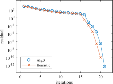
Figure 1: Comparison of Algorithm 3 with heuristic

We now compare the semismooth^∗ Newton method with several first-order splitting method, namely the Forward-Backward splitting method FB, the golden ratio algorithm aGRAAL [12], the Douglas-Rachford splitting algorithm DR and the hybrid projection-proximal point algorithm PM [19]. We performed this comparison only for the scenario with $(n,m)=(200,5)$, where one evaluation of the proximal mapping is relatively cheap, i.e., we have to solve 200 quadratic programs with 10 variables. We generated 3 test problems and computed with the semismooth^∗ Newton method a fairly accurate approximation $\tilde{x}$ of the exact solution: For each of the 3 test problems the final residual was less than $2.4\times 10^{-12}$. Using this approximate solution $\tilde{x}$, we computed for the aforementioned methods the relative error of the iterates $x^{(k)}$ defined as $\max\{\frac{|x_{i}^{(k)}-\tilde{x}_{i}|}{\max\{1,|\tilde{x}_{i}|\}}\,\mid\,i=1,\ldots,nm\}$. In Figure 2 we plot this relative error against the CPU-time needed for calculating $x^{(k)}$. We set for the first-order methods as a time limit five times the time needed for the semismooth^∗ Newton method to converge.

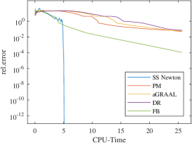
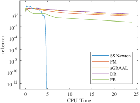
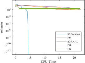
Figure 2: Comparison of the semismooth^∗ Newton method with several first-order methods

We can see that only for the first test problem the FB method was able to produce an approximate solution with high accuracy within the time limit. For the FB method, the final relative error was less than $10^{-5}$, the other methods terminated with a relative error in the range between $4\%$ and $7\%$. For the second test problem, the relative accuracy of the final iterate for the FB-method was about $8\%$, whereas we could not get even one significant digit with the other methods. For the third test problem, the relative error was for all first-order methods about $100\%$.

8 Conclusion

The semismooth^∗ Newton method from [3] and its SCD variant from [4] provide us with a powerful tool for numerical solution of a broad class of problems governed by GEs. When facing a concrete problem of this sort, one has to employ appropriate results of variational analysis in order to implement the AS and the NS in an efficient way. In this paper we suggest an implementation of the SCD semismooth^∗ Newton method for the case of variational inequalities of the 2nd kind, which is a useful modelling framework for a number of practical problems. In particular, in this way one can model Nash games with convex, possibly nonsmooth costs, frequently arising, e.g., in economics and biology. Without substantial changes this implementation can be adopted also to the case of the so-called hemivariational inequalities, cf. [15], which are frequently used in various models in nonsmooth mechanics. This could be a topic for a future research.

References

- [1] F. Facchinei, J.-S. Pang, Finite-Dimensional Variational Inequalities and Complementarity Problems, vol. I+II, Springer, New York, 2003.
- [2] S.D. Flåm, Games and cost of change, Ann. Oper. Res. 301 (2021), pp. 107–-119.
- [3] H. Gfrerer, J. V. Outrata, On a semismooth* Newton method for solving generalized equations, SIAM J. Optim. 31 (2021), pp. 489–517.
- [4] H. Gfrerer, J. V. Outrata, On (local) analysis of multifunctions via subspaces contained in graphs of generalized derivatives, J. Math. Annal. Appl. (2022), https://doi.org/10.1016/j.jmaa.2021.125895
- [5] H. Gfrerer, J. J. Ye, New constraint qualifications for mathematical programs with equilibrium constraints via variational analysis, SIAM J. Optim., 27 (2017), pp. 842–865.
- [6] R. Glowinski, Numerical Methods for Nonlinear Variational Problems, Springer, New York, 1984.
- [7] P. E. Gill, W. Murray, M. H. Wright, Practical Optimization, Academic Press, London, 1981.
- [8] J. Haslinger, M. Miettinen, P. D. Panagiotopoulos (eds.), Finite Element Method for Hemivariational Inequalities. Theory, Methods and Applications, Kluwer, Dordrecht, 1999.
- [9] K. Ito, K. Kunisch, On a semi-smooth Newton method and its globalization, Math. Program., 118 (2009), pp. 347–370.
- [10] A. Jourani, Radiality and semismoothness, Control and Cybernetics 36 (2007), pp. 669–680.
- [11] C. Kanzow, A. Schwartz, Spieltheorie, Springer Nature, Cham, 2018.
- [12] Y. Malitsky, Golden ratio algorithms for variational inequalities, Math. Program. 184 (2020), pp. 383–410.
- [13] F. H. Murphy, H. D. Sherali, A. L. Soyster, A mathematical programming qpproach for determining oligopolistic market equilibrium, Math. Program., 24 (1982), pp. 2–106.
- [14] J. V. Outrata, J. Valdman, On computation of optimal strategies in oligopolistic markets respecting the cost of change, Math. Meth. Oper. Res. 92, 489–509 (2020).
- [15] J. Haslinger, M. Miettinen, P. D. Panagiotopoulos, Finite Element Method for Hemivariational Inequalities: Theory, Methods and Applications, Kluwer Academic Publishers, Boston, Dordrecht, London, 1999.
- [16] S. M. Robinson, A point-of-attraction result for Newton’s method with point-based approximations, Optimization, 60 (2011), pp. 89-99.
- [17] R. T. Rockafellar, Convex analysis, Princeton, New Jersey, 1970.
- [18] R. T. Rockafellar, R. J.-B. Wets , Variational Analysis, Springer, Berlin, 1998.
- [19] M. V. Solodov, B. F. Svaiter, A hybrid projection–proximal point algorithm, J. Conv. Anal. 6(1999), pp. 59–70.
- [20] X. Xiao, Y. Li, Z. Wen, L. Zhang, A Regularized Semi-Smooth Newton Method with Projection Steps for Composite Convex Programs, J. Sci. Comput., 76 (2018), pp. 364–389.