Building separable approximations for quantum states via neural networks

Abstract

Finding the closest separable state to a given target state is a notoriously difficult task, even more difficult than deciding whether a state is entangled or separable. To tackle this task, we parametrize separable states with a neural network and train it to minimize the distance to a given target state, with respect to a differentiable distance, such as the trace distance or Hilbert–Schmidt distance. By examining the output of the algorithm, we obtain an upper bound on the entanglement of the target state, and construct an approximation for its closest separable state. We benchmark the method on a variety of well-known classes of bipartite states and find excellent agreement, even up to local dimension of $d=10$, while providing conjectures and analytic insight for isotropic and Werner states. Moreover, we show our method to be efficient in the multipartite case, considering different notions of separability. Examining three and four-party GHZ and W states we recover known bounds and obtain additional ones, for instance for triseparability.

I Introduction

Entanglement is now considered a defining feature of quantum theory, with broad implications in modern physics, from quantum information processing to many-body physics.

The detection and characterisation of entanglement is however a notoriously challenging problem Horodecki et al. (2009); Gühne and Toth (2009). First of all, it is known that the problem of determining whether a given density matrix is entangled or separable is NP-hard Gurvits (2003); Gharibian (2010). There exist however general methods for detecting entanglement, notably the celebrated negativity under partial transposition (NPT) criteria which ensures the considered density matrix must be entangled Peres (1996); Horodecki et al. (1996). The converse, however, does not hold, as there exist entangled states which are positive under partial transposition, so-called bound (or PPT) entanglement Horodecki et al. (1998). Other techniques have been developed, yet all of them are only useful in specific cases in practice. In particular, Ref. Navascués et al. (2009) developed a method based on semi-definite programming, while Refs Barreiro et al. (2010a); Kampermann et al. (2012) proposed a numerical algorithm to construct separable decompositions. Moving beyond the bipartite case, the certification of multipartite entanglement, of which there exist a zoology of different forms, is by far even more challenging and less understood.

Beyond the question of determining whether a given quantum state is entangled or not, one may consider the problem of approximating a given target state via a separable one. More precisely, if the target state is separable, the question is to provide an explicit (separable) decomposition for the density matrix. While, if the state is entangled, to construct a separable state that minimizes a certain distance (in the Hilbert space) with respect to the target state.

This question has been addressed indirectly in the studies of entanglement measures based on the distance from the set of separable states Horodecki et al. (2009); Vedral et al. (1997), and is particularly relevant when constructing entanglement witnesses Pittenger and Rubin (2002); Bertlmann et al. (2002a); Pittenger and Rubin (2003); Bertlmann et al. (2005a); Bertlmann and Krammer (2008). Additionally, finding the closest separable state has been studied directly, but this task is even difficult for two-qubit systems Kim et al. (2010). For a very specific notion of distance, it has also been studied directly though the concept of “best separable approximation” of a quantum state Lewenstein and Sanpera (1998). The construction of separable approximations for multipartite states is largely unexplored, except for specific families of states, which typically have a high level of symmetry Ishizaka (2002); Hayashi et al. (2008, 2009); Hübener et al. (2009); Parashar and Rana (2011); Carrington et al. (2015); Quesada and Sanpera (2014); Akulin et al. (2015); Rodriques et al. (2014). Moreover, Ref. Shang and Gühne (2018) developed a numerical method based on Gilbert’s algorithm for constructing closest separable approximations for multipartite states, considering various notions of separability.

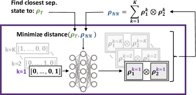
Figure 1: Schematic of the proposed algorithm. Given a target state $\rho_{\text{T}}$, a neural network constructs a separable state $\rho_{\text{NN}}$ which minimizes the distance to the target, i.e. it tries to find the closest separable state. For a single input $k$ (represented in the one-hot encoding), the neural network outputs the (subnormalized) pure state $\rho_{1}^{k}\otimes\rho_{2}^{k}$. The neural network is evaluated for $K$ values of $k$, and its outputs are summed up to construct $\rho_{\text{NN}}$. The distance between this and $\rho_{\text{T}}$ is used to update the neural network’s parameters.

In the present work, we attack these questions using tools from machine learning. Specifically, we devise neural networks for constructing a separable approximation, given a target density matrix. We define a notion of “closest separable state”, which represents the separable state minimizing a given distance with respect to the target; note that this does not coincide with the best separable approximation in general. We benchmark our method with two distance measures, the trace distance and Hilbert-Schmidt distance, on several examples, including bipartite entangled state of local dimension up to $d=10$ (isotropic and Werner states). From the output of the algorithm, we obtain some analytical insight on the distance to the closest separable state as well as its structure. We also consider a family of states featuring bound entanglement. In turn, we demonstrate the potential of our method in the multipartite case, where we construct multi-separable decompositions for several classes of entangled states (noisy GHZ and W states) up to four qubits. Again, we show how to obtain some analytical bounds on the noise thresholds from the output of the algorithm. In particular, we establish estimates on multi-separability. We conclude with a number of open questions and directions for future research. Finally, in the Appendices we study the case of randomly chosen two-qubit states, for which we create ansätze for closest separable states, and derive an exact bound for the two-qubit case.

II Related work

Previous work on using machine learning for the separability problem has been focused either having the machine choose good measurements and then using an existing entanglement criteria Wang (2017); Yosefpor et al. (2020) , or on viewing the task as a classification problem Lu et al. (2018); Gao et al. (2018); Ma and Yung (2018); Gray et al. (2018); Yang et al. (2019); Goes et al. (2021); Ren and Chen (2019). For classification, typically a training set is constructed where quantum states are labeled as separable or entangled. The machine learns on this training set and given a new example predicts whether it is entangled or separable. There are several difficulties with this approach. First, the machine just gives a guess of whether the state is entangled or separable, and does not provide any kind of certificate. Second, the training data can only be generated in a regime where we already understand the problem well, which results in the machine giving only marginal new insight at best. This could be circumvented by using suboptimal criteria (e.g. PPT) to create the training data, however, the machine would just learn this criteria instead of correctly identifying the entanglement and/or separability boundary.

We overcome these challenges by using a generative model, which tries to give an explicit separable decomposition of a target state. This way, we immediately get a certified upper bound on the distance from the separable states. A similar approach has been taken in Refs. Harney et al. (2020, 2021), where the authors represent the quantum states with “quantum neural network states” Carleo and Troyer (2017); Melko et al. (2019), and their extension to density matrices Yoshioka and Hamazaki (2019); Hartmann and Carleo (2019); Nagy and Savona (2019); Vicentini et al. (2019), as opposed to the dense representation we utilise. Their results show a more limited flexibility in the loss function and in the design of types of separable states, in particular in the multipartite case. In contrast, our technique allows us to examine the key notion of genuine multipartite entanglement Horodecki et al. (2009); Gühne and Toth (2009), the strongest form of entanglement in multipartite quantum systems. This is possible as our model allows for optimising over biseparable models. Hence we can obtain close to optimal bounds for demonstrating 3-party and 4-party genuine multipartite entanglement. Moreover, our method also allows us to tackle the even harder question of triseparability.

III Preliminaries

In this section we first introduce the notions of separability for bipartite and multipartite systems and then define the closest separable state. Finally we introduce the basic concepts of neural networks. For more detailed introductions on separability and entanglement or on neural networks, we refer the interested reader to Refs. Horodecki et al. (2009) and Goodfellow et al. (2016), respectively.

A quantum state $\rho_{12}$ acting on $\mathscr{H}_{1}\otimes\mathscr{H}_{2}$, shared between two parties, is said to be separable if it can be constructed by the convex combination of some local quantum density matrices $\rho_{1}^{k}$ acting on $\mathscr{H}_{1}$, and $\rho_{2}^{k}$ acting on $\mathscr{H}_{2}$ as

$$\rho=\sum_{k=1}^{K}p_{k}\rho_{1}^{k}\otimes\rho_{2}^{k},$$ (1)

with $\{p_{k}\}_{k}$ a normalized discrete probability distribution. Any state which is not separable is entangled. For finite dimensional systems, i.e. where $d_{i}:=\text{dim}(\mathscr{H}_{i})<\infty$, for $i\in\{1,2\}$, the local states of the decomposition, $\rho_{i}^{k}$, can be taken to be pure. Due to Caratheodory’s theorem, the number of terms required in the sum, $K$, is upper bounded by $(d_{1}d_{2})^{2}$.

For a multipartite system of $n$ parties several notions of separability exist. The straightforward generalization of Eq. (1) results in the notion of a fully separable decomposition,

$$\rho=\sum_{k=1}^{K}p_{k}\rho_{1}^{k}\otimes\rho_{2}^{k}\otimes\dots\otimes\rho_{n}^{k}.$$ (2)

Naturally, one can also just examine bipartite separability on the mutlipartite system by grouping the parties together. This leads to the notion of biseparability with respect to the partition $(\mathscr{I}|\mathscr{\bar{I}})$,

$$\rho=\sum_{k=1}^{K}p_{k}\rho_{\mathscr{I}}^{k}\otimes\rho_{\bar{\mathscr{I}}}^{k},$$ (3)

where $\mathscr{I}$ denotes a subset of the indices $\{1,2,\dots,n\}$ and $\bar{\mathscr{I}}$ denotes its complement. A multipartite state is called biseparable if it can be decomposed as a convex mixture of states that are separable considering all possible bipartitions, namely

$$\rho=\sum_{k=1}^{K}p_{k}\rho_{\mathscr{I}_{k}}^{k}\otimes\rho_{\bar{\mathscr{I}_{k}}}^{k},$$ (4)

where crucially, now each $I_{k}$ can be different.

There are many ways to quantify entanglement of a target state $\rho_{\text{T}}$, among which a particularly useful one is based on the distance of a state from the set of separable states. Any distance measure $D$ between quantum states $\sigma_{1},\sigma_{2}$, which is zero if and only if $\sigma_{1}=\sigma_{2}$, and for which $D(\sigma_{1},\sigma_{2})\geq D\left(\Lambda(\sigma_{1}),\Lambda(\sigma_{2})\right)$ for any completely positive trace preserving map $\Lambda$, can be used to construct an entanglement measure, by minimizing $D(\rho_{\text{T}},\rho_{\text{Sep.}})$ over separable states $\rho_{\text{Sep.}}$ Horodecki et al. (2009); Vedral et al. (1997). We will use the neural network to find the closest separable state with respect to a distance $D$, formally

$$\rho_{\text{CSS}}:=\underset{\rho_{\text{Sep}}}{\arg\min}\,D(\rho_{\text{T}},\rho_{\text{Sep.}})),$$ (5)

where $\rho_{\text{Sep}}$ is a separable state. Note that the closest separable state is not necessarily unique. For the neural network method presented in this paper, any $D$ which is differentiable with respect to one of the states can be used. We choose to work with two distances; the first is the trace distance (related to the Schatten 1-norm) Eisert et al. (2003),

$$D_{\text{Tr}}(\sigma_{1},\sigma_{2})=\frac{1}{2}\text{Tr}\sqrt{(\sigma_{1}-\sigma_{2})^{2}}=\frac{1}{2}\sum_{i}|\mu_{i}|,$$ (6)

where $\{\mu_{i}\}_{i}$ are the eigenvalues of $\sigma_{1}-\sigma_{2}$. Note that the trace-distance-based measure can be useful in quantum hypothesis testing, and, among other measures, is an important measure in the study of closest classical states, which is distinct from the closest separable state Aaronson et al. (2013); Paula et al. (2013); Nakano et al. (2013); Modi et al. (2010); Bellomo et al. (2012). We will not examine closest classical states in this work, but note that our methods can easily be adopted for their study.

The second distance we consider is the Hilbert-Schmidt distance (related to the Schatten 2-norm) Vedral and Plenio (1998); Witte and Trucks (1999); Krammer (2009)

$$D_{\text{HS}}(\sigma_{1},\sigma_{2}) =\sqrt{\text{Tr}\left[(\sigma_{1}-\sigma_{2})^{2}\right]}.$$ (7)

The Hilbert–Schmidt-based measure can be useful for constructing entanglement witnesses Pittenger and Rubin (2002); Bertlmann et al. (2002a); Pittenger and Rubin (2003); Bertlmann et al. (2005a); Bertlmann and Krammer (2008). Both the trace distance and Hilbert-Schmidt distance can be used as a basis for an entanglement measure, however, one could consider others, such as the Bures distance Vedral and Plenio (1998), relative entropy of entanglement Vedral et al. (1997) or the robustness of entanglement Vidal and Tarrach (1999); see e.g. Ref. Zyczkowski and Bengtsson (2006) for an overview and other examples of geometric measures of entanglement.

Let us now concisely introduce the concept of an artificial neural network Goodfellow et al. (2016), the basis of our numerical representation of separable states. A neural network is a numeric model which can in principle represent any multivariate function. A crucial point is to be able to adjust the parameters of the neural network to represent the desired function, however in many use-cases this can be done surprisingly efficiently with the techniques of deep learning.

In this work we will be using one of the simplest types of neural networks, the so-called multilayer perceptron. It is characterized by the number of neurons per layer (width), the number of layers (depth), and the activation functions used at the neurons. Altogether these model an iterative sequence of parametrized affine, and fixed nonlinear transformations, on the input; namely the map from layer $l$ to $l+1$ is

$$r_{l+1}=h(W_{l}r_{l}+b_{l}),$$ (8)

where the weight matrix $W_{l}$ and bias vector $b_{l}$ parametrize the affine transformation, $h$ is a fixed differentiable nonlinear function (activation function), and $r_{l}$ is the input of layer $l$, and its length signifies the width (number of “neurons”) of layer $l$. The vector $r_{1}$ ($r_{\text{depth}}$) is the input (output) of the whole model. At initialization, the weights and biases of all layers are set randomly. During training, the parameters of the model ($\{W_{l},b_{l}\}_{l}$) are updated such that they minimize a differentiable loss function of the training set, which as we will see later, in our case will be the trace or Hilbert–Schmidt distance. This is done by first evaluating the model for a batch of inputs, and then by slightly updating the parameters via a method called backpropagation, which relies on the gradient of the loss function with respect to the model parameters. This is repeated for many batches, until the model converges, a maximum training time is reached, or a satisfactory loss is achieved. Once trained, the neural network can be evaluated on new input instances.

IV Neural networks as separable states

The task is to find the closest separable state to a given target density matrix. The central idea of this work is to use a neural network as a variational ansatz for the density matrix by representing the local components of the separable decomposition with a single neural network. The approach is inspired by a similar approach taken for nonlocality, where neural networks represent the local components of a Bell-local behavior Kriváchy et al. (2020).

To demonstrate the method, let us examine the example of a bipartite 2-qubit state. We ask a neural network to represent the map

$$k\rightarrow(p_{k},\rho^{k}_{1},\rho^{k}_{2}),$$ (9)

where we take $\rho^{k}_{i}={\lvert\psi^{k}_{i}\rangle}{\langle\psi^{k}_{i}\rvert}$ to be pure states, with ${\lvert\psi^{k}_{i}\rangle}=\alpha^{k}_{i}{\lvert 0\rangle}+\beta^{k}_{i}{\lvert 1\rangle}$. That is, the neural network will take as input an integer value $k$ between $1$ and $K$ (in a one-hot representation), and will output the numbers $(p_{k},\alpha^{k}_{1},\beta^{k}_{1},\alpha^{k}_{2},\beta^{k}_{2})$, such that normalization for each subsystem is satisfied. Note that for each complex number, two real numbers are output, the real and imaginary part. We evaluate the neural network for $K$ values of $k$, normalize the $(p_{k})_{k}$ probability vector and sum up the outputs $p_{k}\rho^{k}_{1}\otimes\rho^{k}_{2}$ to construct a separable state via Eq. (1), namely $\rho_{\text{NN}}=\sum_{k=1}^{K}p_{k}\rho^{k}_{1}\otimes\rho^{k}_{2}$. The neural network is trained to minimize the distance between the target density matrix $\rho_{\text{T}}$ and the constructed separable density matrix $\rho_{\text{NN}}$, i.e. $D_{\text{Tr}}(\rho_{\text{T}},\rho_{\text{NN}})$. The process is roughly illustrated in Fig. 1, where the $p_{k}$ are not shown explicitly.

By construction the neural network represents a single density matrix $\rho_{\text{NN}}$, so for each target state $\rho_{\text{T}}$, the network must be retrained in order to obtain an approximation of the closest separable state to that target state. During training, requiring $K$ values of $k$ in order to evaluate the state technically means working with a batch size of size $K$. That is, we evaluate $K$ inputs ($k=1,2,\dots K$) to construct $\rho_{\text{NN}}$ and only then calculate the gradients required for the optimization of the neural network. An advantage of this method is that only the input layer increases with $K$, which implies that the global size of the neural network can grow slowly with the dimension of the target state.

More generally, for more parties or higher dimensions, the neural network represents the map

$$k\rightarrow(p_{k},\rho^{k}_{1},\rho^{k}_{2},\dots\rho^{k}_{n}),$$ (10)

where we take the $\rho^{k}_{i}$ ($i=1\dots n$) to be pure, and the neural network explicitly outputs the parameters of the pure states. By evaluating this neural network for $K$ values of $k$, we construct a separable state via either Eq. (1) for the bipartite case ($n=2$), or any of Eqs. (2,3,4) for the different notions of multipartite separability. Recall that by Caratheodory’s theorem, in principle the largest $K$ needed is $\prod_{j}d_{j}^{2}$, however even less could be sufficient. Thus we keep $K$ as a free hyperparameter, which we set before training begins. More technical details on the neural networks we used can be found in Appendix A or in the sample code provided in the Code Availability section.

The neural network is optimized in the high-dimensional non-convex landscape of the network’s weights, so it is not guaranteed to converge to the optimal solution. However, in practice, optimization procedures based on gradient descent reach close-to-optimal solutions efficiently. Notice, that even for suboptimal solutions we obtain an upper bound on the amount of entanglement of the target state, since the utilized distances serve as entanglement measures Vedral et al. (1997); Vedral and Plenio (1998); Horodecki et al. (2000). However, we can go one step further, and examine families of states parametrized by a single parameter, which we refer to as $q$, typically of the form

$$\rho_{\text{T}}(q)=q\rho_{\text{ent}}+(1-q)\rho_{\text{sep}},$$ (11)

where $\rho_{\text{ent}}$ is an entangled state and $\rho_{\text{sep}}$ is a separable state, oftentimes the maximally mixed state. If $\rho_{\text{ent}}\equiv\rho_{\text{T}}(q=1)$ is truly entangled, then when decreasing $q$, for some value $q^{*}$ we will cross the separability boundary. We can observe this transition by varying $q$ and retraining the neural network from scratch for each target distribution. An approximation of $q^{*}$ becomes clear from how close the algorithm can get to the target states for different $q$ values.

V Case studies

To benchmark the method, we first use the algorithm to examine the separability boundary for some exemplary families of bipartite states. We consider symmetric classes of states, i.e. isotropic and Werner states, and estimate the noise threshold for separability. We find excellent agreement with analytically known optimal thresholds. Additionally, we compare our results for the minimal Hilbert-Schmidt distance for isotropic states to the known analytic distance, and find excellent correspondence. We furthermore conjecture the minimal trace distances for isotropic, and trace and Hilbert-Schmidt distances for Werner states. Moreover, we obtain analytical insight to the problem of characterising the closest separable states for the Bell state in terms of trace distance. Then we also discuss an example of bound entanglement, i.e. an entangled sate that cannot be detected by the partial transpose criterion.

Then we move on to the multipartite case, where we consider 3- and 4-qubit GHZ and W states. We show that our algorithm can capture various notions of multipartite entanglement, including full separability, biseparability and even triseparability. We estimate again noise thresholds, finding excellent agreement with previously known bounds. Moreover, we explain how, from the numerical output from the algorithm, one can obtain analytical bounds on the noise thresholds.

Additionally, in Appendix B we compare our neural network algorithm to a naive gradient-descent based heuristic to show its advantage. In Appendix C we examine the performance of the algorithm on random bipartite two-qubit density matrices, and compare it to the optimal solution obtained via a semi definite program (SDP). We conjecture an analytic ansatz of the closest separable state for a general 2-qubit state, which we find to be very close to the solutions found by the neural network, and prove a bound on the trace distance. In Appendix D, we detail a method to obtain a strict lower bound on the separability threshold compatible with our method.

V.1 Bipartite case

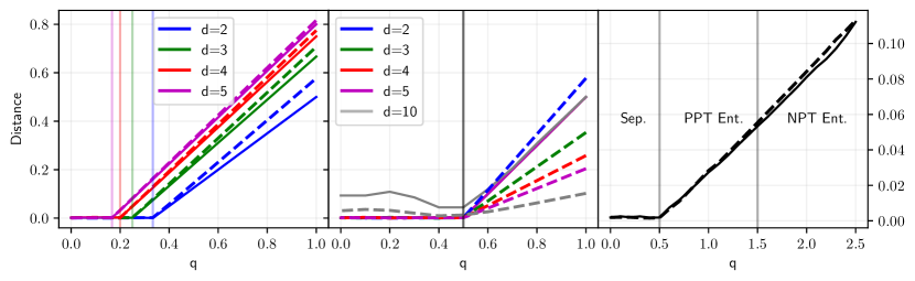
Figure 2: Distance from target state to closest separable state found by the neural network, trained and evaluated on the trace distance (solid lines) or Hilbert–Schmidt distance (dashed lines), trained independently for different values of $q$. Separability thresholds are depicted with vertical lines. Results are shown for $d\times d$ isotropic (left) and Werner (center) states, as well as for PPT entangled states of the form (20) (right). Note that for the Werner states with $2\leq d\leq 5$, all the trace distance curves essentially overlap and are thus not distinguishable on the plot. For the right plot we did 2 runs and kept the best results to improve the smoothness of the curves.

We start our benchmarking with two classes of highly symmetric bipartite states. Isotropic states are defined as

$$\rho_{\text{iso}}(q)=\frac{1-q}{d^{2}}\mathbb{I}_{12}+q{\lvert\phi^{+}_{d}\rangle}{\langle\phi^{+}_{d}\rvert},$$ (12)

where $0\leq q\leq 1$, $\mathbb{I}_{12}$ is the identity operator on the joint space, and

$${\lvert\phi^{+}_{d}\rangle}=\frac{1}{\sqrt{d}}\sum_{i=1}^{d}{\lvert i\rangle}_{1}{\lvert i\rangle}_{2},$$ (13)

is the maximally entangled state of local dimension $d$. Werner states are defined as

$$\rho_{\text{Werner}}(q)=(1-q)\frac{2}{d(d+1)}P_{\text{sym}}+q\frac{2}{d(d-1)}P_{\text{as}},$$ (14)

where

$$P_{\text{sym}}= \frac{1}{2}(\mathbb{I}_{12}+F_{12}),$$

$$P_{\text{as}}= \frac{1}{2}(\mathbb{I}_{12}-F_{12}),$$

with $F_{12}=\sum_{i,j}^{d}{\lvert i\rangle}{\langle j\rvert}_{1}\otimes{\lvert j\rangle}{\langle i\rvert}_{2}$ the flip operator.

These classes of states represent a good benchmark as the separability thresholds, i.e. the value of $q$ for which the state becomes separable, are known analytically. Specifically, isotropic states are separable for $q\leq\frac{1}{d}$, while Werner states are separable for $q\leq\frac{1}{2}$. Hence when running our algorithm for these classes of target states, for different values of $q$, we expect to find a distance of the closest separable state that vanishes when $q$ approaches the separability threshold. This is precisely what we observe. We run the neural network independently for 11 values of $q$, and additionally for the exact separability boundary value. The results for both the trace distance and Hilbert-Schmidt distance for $d\leq 5$ are depicted in Fig. 2 (each line is plotted with its respective loss function, the trace or Hilbert-Schmidt distance). They confirm that the algorithm works properly in this regime, finding a sharp transition at the known separability thresholds. When making a linear fit to the data that is outside the seemingly flat separable region, we recover the thresholds with a precision of at least $10^{-4}$. To give an example of the running time on a personal computer, for isotropic states the training for a single target state for $d=5$ took at most 15 minutes, while for $d=2$ it took only at most 30 seconds. When the trace distance is found to be smaller than $2\cdot 10^{-3}$, we choose to stop the training, and conclude that the state to be separable. Otherwise we run the algorithm until the resulting trace distance converges, i.e. it doesn’t change more than $2\cdot 10^{-4}$ in one epoch.

Additionally, for $d=10$ we examine the Werner states, also plotted in Fig. 2. For such a large state, with $K=100$, training took about 1 hours 15 minutes on a personal computer for a single epoch (3000 batches), which was reduced to 45 minutes when training on a GPU. Due to the increased runtime we only ran one epoch for each point in Fig. 2, and did not wait until convergence. We observe that the neural network struggles more in finding a closest separable state in the separable area, however it works remarkably well in the entangled regime, and still manages to give qualitatively interpretable results on where the entanglement boundary lies. For increased accuracy one could run the algorithm several times independently and take the smallest value for each $q$, or one could run the algorithm with a larger batch size $K$. For example for the separability boundary at $q=0.5$, by using $K=150$ instead of 100, after 5 epochs (5 times 3000 batches), the trace distance reduced to 0.024 from the 0.045 seen in Fig. 2.

For isotropic states, the exact Hilbert-Schmidt distance to the closest separable state is known. In dimension 2, we retrieve the value of $1/\sqrt{3}$ that was known shown in Refs. Witte and Trucks (1999); Bertlmann et al. (2002a). A generalized formula is given by Ref. Bertlmann et al. (2005a),

$$D_{\text{HS}}^{\text{iso}}=\frac{\sqrt{d^{2}-1}}{d}\left(q-\frac{1}{d+1}\right),$$ (15)

which we recover up to excellent precision for $q=1$ and up to $d=10$ in Fig. 3.

Moreover, we examine the trace distance, and based on the results in Figs. 2 and 3, we conjecture that the trace distance from the isotropic states to their respective closest separable states follows

$$D_{\text{Tr}}^{\text{iso}}=\frac{d^{2}-1}{d^{2}}\left(q-\frac{1}{d+1}\right).$$ (16)

Using the semidefinite program described in Appendix C, we can verify that a trace distance of $1/2$ is optimal for the Bell state, i.e. for $d=2$. We have not found this explicitly proven in the literature, even though the related concept of finding the closest classical state to the Bell state has been well studied Paula et al. (2013); Nakano et al. (2013); Aaronson et al. (2013).

For Werner states, similarly drawing from Fig. 2, we conjecture that the distance to the closest separable is given by

$$D_{\text{HS}}^{\text{Wer}}=\frac{2}{\sqrt{d^{2}-1}}\left(q-\frac{1}{2}\right)$$ (17)

for the Hilbert-Schmidt distance, and by

$$D_{\text{Tr}}^{\text{Wer}}=q-\frac{1}{2}\,,$$ (18)

for the trace distance. To the best of our knowledge, these relations are not proven in the literature. We note that plotting these conjectured equations in Fig. 2 (first two panels) would result in lines that are indistinguishable from the data.

While the algorithm performs a numerical optimisation, one can nevertheless obtain some analytical insight from the output. Here we illustrate this point. First we could partially characterize the closest separable state for the two-qubit Bell state, i.e. ${\lvert\phi^{+}_{2}\rangle}$. Setting the Bell state as the target, and using the trace distance as the loss function of the neural network, at the end of training it finds the separable state

$$\begin{pmatrix}(\frac{1}{2}-a)&c&\bar{c}&a\\ \bar{c}&a&b&-\bar{c}\\ c&\bar{b}&a&-c\\ \bar{a}&-c&-\bar{c}&(\frac{1}{2}-a)\end{pmatrix},$$ (19)

with $a=\frac{1}{4}$, $|b|\in[0,1/4]$ and small $c$ values. However, when using the Hilbert–Schmidt distance $D_{\text{HS}}$ as the loss, the neural network converges to the $a=\frac{1}{6}$, $b=0$ and $c=0$ solution. Both solutions have the same trace distance of $0.5$ from the Bell state. From these two extremes, we constructed the ansatz Eq. 19 for the closest separable state and verify that for $c=0$, $a\in[0,\frac{1}{6}]$ and $b\in[0,a]$ they indeed all give a trace distance of $\frac{1}{2}$. We go further and find other values of $(a,b,c)$ for which the trace distance is $\frac{1}{2}$. For example if all parameters are set to be real, and $b=a$, then it is a closest separable state for $\sqrt{(a-\frac{1}{8})^{2}+c^{2}}\leq\frac{1}{8}$. The same holds for $a=1/6$, $24c^{2}-\frac{1}{6}\leq b\leq\frac{1}{6}$ (with all parameters real). Clearly there are countless others, but characterizing the whole range of satisfactory $(a,b,c)$ values is beyond the scope of this paper. This analysis stands here to show how one can gain insight by looking at the output state of the neural network.

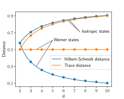
Figure 3: Distance to the closest separable state for the maximally entangled state ${\lvert\phi^{+}_{d}\rangle}$ (i.e. an isotropic state with $q=1$) and the Werner state as a function of the local dimension $d$. The dots indicate the values found by the neural network. For the Hilbert-Schmidt distance (blue curve), Eq. (15) gives the exact expression for the isotropic state as proven in Ref. Bertlmann et al. (2005a). We conjecture the general formula for the trace distance of the isotropic state in Eq. (16). For the Werner states, we conjecture the general formula for the trace distance in Eq. (17) and for the Hilbert-Schmidt distance in Eq. (18).

To conclude our discussion of the bipartite case, we consider a family of entangled states that feature bound entanglement. Specifically, we consider the class of states introduced in Ref. Witte and Trucks (1999), although we adopt the parametrization used in Ref. Mintert et al. (2005). This family of 2-qutrit states exhibits bound entanglement, i.e. a PPT entangled region. The states are

$$\rho_{q}=\dfrac{1}{21}\begin{pmatrix}2&0&0&0&2&0&0&0&2\\ 0&\beta_{-}&0&0&0&0&0&0&0\\ 0&0&\beta_{+}&0&0&0&0&0&0\\ 0&0&0&\beta_{+}&0&0&0&0&0\\ 2&0&0&0&2&0&0&0&2\\ 0&0&0&0&0&\beta_{-}&0&0&0\\ 0&0&0&0&0&0&\beta_{-}&0&0\\ 0&0&0&0&0&0&0&\beta_{+}&0\\ 2&0&0&0&2&0&0&0&2\end{pmatrix},$$ (20)

with $\beta_{\pm}=\dfrac{5}{2}\pm q$, and $q\in[-2.5,2.5]$, however, we only consider $q\in[0,2.5]$ since the negative $q$ regime gives the same states up to permutations. It is known that $\rho_{q}$ is separable for $q\in[0,0.5]$, is PPT entangled for $q\in(0.5,1.5]$ and is NPT entangled for $q\in(1.5,2.5]$. For several values of $q$ we train the neural network to approximate $\rho_{\text{T}}=\rho_{q}$, and display the results in Fig. 2. We can see that by explicitly constructing the separable decomposition, our results are not sensitive to whether the partial transpose is positive or negative, and the neural network approach successfully identifies the separable and entangled regions.

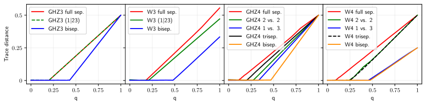
Figure 4: Neural network run on three and four-qubit GHZ and W states for different $q$ values, and different separable models. See Tables 1 and 2 for the extracted threshold estimates. The 3-qubit GHZ full separability and (1|23) separability, as well as the 4-qubit W biseparability and 1 vs. 3 biseparability, and triseparability and 2 vs. 2 biseparability curves almost completely overlap, making them difficult to distinguish on the plot.

V.2 Multipartite case

We now consider three and four qubit multipartite states by examining the exemplary GHZ and W states, mixed with white noise. The GHZ state is

$${\lvert\text{GHZ}\rangle}=\frac{1}{\sqrt{2}}\left({\lvert 00\dots 0\rangle}+{\lvert 11\dots 1\rangle}\right),$$ (21)

while the W state is

$${\lvert\text{W}\rangle}=\frac{1}{\sqrt{n}}\left(({\lvert 0\dots 01\rangle}+{\lvert 0\dots 10\rangle}+\dots+{\lvert 10\dots 0\rangle}\right).$$ (22)

We mix both with the maximally mixed state as we did for the isotropic states in Eq. (12). For three qubits, we use the neural network to distinctly examine

1. full separability, as in Eq. (2) ($n=3$),

2. biseparability with respect to a single partition (1$|$23), as in Eq. (3),

3. biseparability, as in Eq. (4),

and for the four qubits,

1. full separability, as in Eq. (2) ($n=4$),

2. biseparability with respect to the partition (12$|$34), as in Eq. (3),

3. biseparability with respect to the partition (1$|$234), as in Eq. (3),

4. biseparability with respect to 2 vs. 2 partitions, i.e. as in Eq. (4), except all partitions $\mathscr{I}_{k}$ are constrained to have 2 parties,

5. biseparability with respect to 1 vs. 3 partitions, i.e. as in Eq. (4), except all partitions $\mathscr{I}_{k}$ are constrained to have 1 party (and thus the complements $\bar{\mathscr{I}}_{k}$ have 3 parties),

6. triseparability, as a generalization of Eq. (4), namely $\rho=\sum_{k}p_{k}\rho_{\mathscr{I}_{k}^{1}}^{k}\otimes\rho_{\mathscr{I}_{k}^{2}}^{k}\otimes\rho_{\mathscr{I}_{k}^{3}}^{k}$, with $(\mathscr{I}_{k}^{1}|\mathscr{I}_{k}^{2}|\mathscr{I}_{k}^{3})$ a partitioning of $\mathscr{I}$ for each $k$, and

7. biseparability, as in Eq. (4).

For the biseparable and triseparable cases, on a technical level, for each $k$ we ask the neural network to output density matrices for all possible partitions, i.e. for each $k$ it actually outputs 3 terms at a time for the 3-party case, and 6 terms for the 4-party case.

We present the results in Fig. 4, except for 4-qubit separability with respect to a fixed partition, to not overcrowd the figure, however, note that those results are qualitatively similar. The consistent straight lines formed from independent runs give us confidence that the algorithm works well for approximately detecting the separability boundaries.

From Fig. 4, we extract estimates of the separability bound by fitting linear curves to the data that is outside the seemingly flat separable region and close to the boundary. Moreover, inspired from Ref. Shang and Gühne (2018), we show how to obtain actual lower bounds on the separability thresholds in Appendix D. All results are given in Tables 1 and 2. With the flexibility of the current technique, we are able to quickly get estimates and bounds on the noise thresholds for many notions of separability, or alternatively, entanglement. These results can be improved by taking more points or running the algorithm multiple times. In cases where the exact threshold is known, our results are close to it. Where the boundary is not known to be exact, we can see how close it is to being tight. We observe that in these cases, in fact the analytic upper bounds seem to be close to, or in fact, optimal. Finally, we established estimates for many notions of separability, for which we did not find previous estimates or bounds in the literature. These were complemented by lower bounds provided by J.Shang and O. Gühne based on the method in Ref. Shang and Gühne (2018) in private communications.

Table 1: Three-party separability thresholds for the noisy GHZ and W states. Previously known bounds are all upper bounds. An asterisk (*) denotes that the bound is known to be exact. Our results are given with an estimation of the bound obtained with a linear fit close to the threshold and with a certified lower bound obtained as discussed in Appendix D.

	3-qubit GHZ			3-qubit W
Separability	Estimate with linear fit	Lower bound	Previous bound	Estimate with linear fit	Lower bound	Previous bound
Full sep.	0.199	0.197	0.2* Dür and Cirac (2000)	0.177	0.177	0.178* Chen and Jiang (2020)
1|23 sep.	0.198	0.198	0.2* Dür and Cirac (2000)	0.206	0.208	0.210 Szalay (2011)
Bisep.	0.428	0.423	0.429* Gühne and Seevinck (2010)	0.478	0.473	0.479*Jungnitsch et al. (2011)

Table 2: Four-party separability thresholds for the noisy GHZ and W states. Results are given as (i) an estimate of the bound obtained via a linear fit close to the threshold and (ii) a certified lower bound obtained from the method discussed in Appendix D. Bounds marked with a dagger ($\dagger$) are lower bounds provided by J.Shang and O. Gühne based on the method in Ref. Shang and Gühne (2018) in a private communication. All other previously known bounds are upper bounds. An asterisk (*) denotes cases where the bound is known to be exact.

	4-qubit GHZ			4-qubit W
Separability	Estimate with linear fit	Lower bound	Previous bound	Estimate with linear fit	Lower bound	Previous bound
Full sep.	0.107	0.101	0.111* Dür and Cirac (2000)	0.086	0.073	0.093* Chen and Jiang (2020)
(12|34)	0.109	0.109	0.111* Dür and Cirac (2000)	0.109	0.109	0.113†
(1|234)	0.108	0.107	0.111* Dür and Cirac (2000)	0.123	0.124	0.128†
2 vs. 2 sep.	0.271	0.267	0.269†	0.239	0.226	0.245†
1 vs. 3 sep.	0.333	0.328	0.327†	0.452	0.435	0.447†
Trisep.	0.198	0.194	0.198†	0.247	0.241	0.243†
Bisep.	0.467	0.451	0.467* Jungnitsch et al. (2011)	0.472	0.458	0.474 Jungnitsch et al. (2011)

VI Conclusion and outlook

In summary, we have addressed the question of constructing the closest separable state to a given target state, by using a neural network as a compact model for separable states. We avoided the bottleneck of having to explicitly model many (up to $\prod_{j=1}^{n}d_{j}^{2}$) separable pure states in a decomposition by using a single neural network to represent them all. We demonstrated that by training the model independently on multiple states from a family, we can identify the separability boundary well. We did this for examples where the boundaries are known, PPT entangled states, as well as 3- and 4-party multi-qubit states. Additionally, we showed how analytical insight can be gained from the output of the algorithm. In the bipartite case, we partially characterized the closest separable state for the two-qubit Bell state, and conjectured relations for the distances in case of arbitrary dimension. In the multipartite case we showed how to obtain strict lower bounds on the noise threshold.

The technique presented here opens up avenues for a variety of numeric applications in quantum foundations. In particular, for any task with reasonable Hilbert space sizes, it is possible to optimize over the set of separable states, as long as the loss function is differentiable. Among other potential applications, it can be especially helpful for obtaining (estimates or bounds on) entanglement measures, measures of robustness, separable ground state energies, and with minor modifications can be easily adapted to finding the closest classical state. Moreover, a particularly fruitful avenue for research could be focused on combining our approach with other generative neural network approaches to quantum state representations, namely “quantum neural network states” Carleo and Troyer (2017); Melko et al. (2019), particularly their extension to density matrices Yoshioka and Hamazaki (2019); Hartmann and Carleo (2019); Nagy and Savona (2019); Vicentini et al. (2019). Using such an ansatz for the separability problem has been examined in Ref. Harney et al. (2021). Such prospects of further developing the algorithms give the promise of exciting novel numerical tools for a broad range of tasks, both for numerical work and gaining analytic insight.

VII Code availibility

We have made sample code available at www.github.com/Antoine0Girardin/Neural-network-for-separability-problem.

VIII Acknowledgments

We thank Pavel Sekatski for discussions, and Otfried Gühne and Jiangwei Shang for pointing out the work of Ref. Shang and Gühne (2018) and for providing additional values for Table II. We acknowledge financial support from the Swiss National Science Foundation (project $2000021\_192244/1$ and NCCR QSIT). T.K. additionally acknowledges funding from the Swiss National Science Foundation Doc.Mobility grant (project P1GEP2_199676).

Appendix A Technical details of the utilized neural networks

The main idea of how we use neural networks can be found in the maintext, while the implemented code can be found in the online repository provided. Here, we briefly describe some of the technical details and hyperparameters that we used.

As described in the maintext we use a feedforward neural network to represent a generic separable state of a fixed dimension and separability structure. We use a multilayer perceptron with rectified linear units as activations, except in the final layer where we use sigmoid activations. The outputs are normalized via a softmax function for the probability vectors, and by dividing by the 2-norm for the complex entries of the pure states. For the calculation in the maintext we employed a single hidden layer, with a width of 100, or 200 for more difficult calculations. The number of elements in the separable decomposition, $K$, is analytically upper bounded by $\prod_{j}d_{j}^{2}$, however in the implementation, typically $K=\prod_{j}d_{j}$ gives satisfactory results and allows for much quicker training. For training we use the Adadelta optimizer.

Appendix B Comparing with gradient descent

To see the advantage of using a neural network, we compare our algorithm with the naive optimization algorithm of gradient descent, for the simplest case of two qubits.

We parametrize the quantum state in a similar way as in Eq. (9), i.e. the free parameters are the $K$ probabilities and the real and imaginary parts of the pure states composing the separable state according to Eq. (1), with $d=2,K=16$. The gradient descent algorithm varies these parameters to minimize the trace distance with respect to a target state, which we chose to be the Bell state, namely Eq. (13), with $d=2$. The gradient descent algorithm was run with an initial learning rate of 1, decreased by a factor of 0.98 each round for 250 rounds, and with a momentum factor of 0.2.

Figure 5: (Left) Trace distance from target Bell state versus iteration of gradient descent optimization for complex-valued (solid blue lines) and real-valued (dashed green lines) density matrices, for 20 independent runs each. The true minimum of 0.5 is depicted as a solid red line, which the neural network reaches up to at about 1E-7 precision; result taken from Fig. 2. (Right) Same plot for the real-valued gradient descent on the isotropic state, Eq. (12), for $d=5$, where the expected closest distance should be 0.8 (which the neural network approaches to 1E-6 precision).

Recall that the neural network, even with one layer, did not have any trouble finding the closest separable state with a trace distance of 0.5. However, as shown in the left panel of Fig. 5, we notice that already for this simple case the gradient descent technique has difficulties in finding the closest state. Somewhat surprisingly, if only real numbers are chosen to represent the state, the gradient descent technique performs better and converges to a good solution. Note that for higher dimensions, e.g. $d=5$, the real-valued gradient descent also has difficulties, as shown in the right panel of Fig. 5.

Appendix C Random states

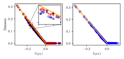
Figure 6: Neural network run on random two-qubit states, with the resulting distances scatter plotted as a function of the smallest eigenvalue of the partial transpose (blue circles). Solid orange lines denote the line of slope -1. (Left) Trained on and plotted with trace distance for 400 samples. Additionally, the ansatz states’ trace distances are depicted with red crosses, and the SDP results are plotted with black horizontal bars. (Right) Trained on and plotted with Hilbert-Schmidt distance for 300 samples.

When benchmarking the method on random states, we noticed that there is a strong connection between the obtained trace distance of the closest separable state and the lowest eigenvalue of the partial transpose. In this appendix, we first show benchmark results for the method on random two-qubit states ($d_{1}=d_{2}=2$), where the PPT criteria clearly distinguishes entangled from separable states. We observe a strong correlation between the trace distance and Hilbert–Schmidt distance of the closest separable state and the smallest eigenvalue of the partial transpose of the state. We verify these results with a SDP to see how close to the optimal solution the neural network can get for two-qubits states. Finally, we present an analytic ansatz of the closest separable state, based on the numerical results of the neural network and our intuition, which we numerically validate to be very close to the actual closest separable state.

In the two-qubit case the positive partial transpose criteria is a necessary and sufficient condition for separability. Thus, in Fig. 6 we plot the distance to the closest separable state obtained by the neural network against the smallest eigenvalue of the partial transpose, which we will refer to as $\lambda$. Using the trace distance as a loss, we tested 400 random states with the trace distance as a loss function, and 300 with the Hilbert–Schmidt distance as the loss (the neural network was retrained 5 times for each state and the lowest distance was kept).

First, we observe that the neural network achieves close to zero distance in the separable regime for all states. Clearly it can not and should not reach zero distance for entangled states (i.e. on the left side of the figures, where $\lambda<0$). We observe a much stronger relation: in fact the Hilbert–Schmidt distances of the closest separable state seem to line up on a line with slope $-1$, while the trace distance results seem to be below this. We formulate these two observations; namely in the entangled regime, for $\lambda(\rho_{\text{T}})<0$,

$$D_{\text{HS}}(\rho_{\text{T}},\rho_{\text{CSS;HS}}) \leq-\lambda(\rho_{\text{T}}),$$ (23)

$$D_{\text{Tr}}(\rho_{\text{T}},\rho_{\text{CSS;Tr}}) \leq-\lambda(\rho_{\text{T}}),$$ (24)

where we explicitly denoted which distance was minimized in the subscript of $\rho_{\text{CSS}}$.

It is possible to use a SDP to find the closest separable state with respect to the trace distance by using the PPT criteria.

The SDP has a dual form and can be expressed as Fazel et al. (2001)

$$\begin{split}&\text{minimize }TrY+TrZ\\ &\text{subject to }\begin{pmatrix}Y&X\\ X^{\dagger}&Z\end{pmatrix}\geq 0\end{split}$$ (25)

With $Y$ and $Z$ Hermitian matrices, $X=\rho_{T}-\rho_{CSS}$, $\rho_{T}$ being the target state and $\rho_{CSS}$ the separable state, $\rho_{CSS}\geq 0$, $tr(\rho_{CSS})=1$, $\rho_{CSS}^{\Gamma}\geq 0$. $\rho_{CSS}^{\Gamma}$ is the partial transpose of $\rho_{CSS}$.

The result of the SDP for all random states are plotted in Fig. 6.

Finally, we provide an ansatz for the closest separable state with respect to the trace distance. Intuitively, we set the smallest eigenvalue of the partial transpose to be 0 instead of negative, and adjust the others such that the trace remains unchanged.

Theorem.

Let $\rho_{\text{T}}$ be an entangled state whose partial transpose has an eigendecomposition of $UDU^{\dagger}$, with $D=\text{diag}(\lambda_{1},\lambda_{2},\lambda_{3},\lambda_{4})$, where $\lambda_{1}$ is the smallest eigenvalue (i.e. $\lambda_{1}\equiv\lambda(\rho_{\text{T}})$). Then let our ansatz of the closest separable state be $\rho^{\prime}=(UD^{\prime}U^{\dagger})^{\Gamma}$ with $D^{\prime}=\text{diag}(0,\lambda_{2}+\frac{\lambda_{1}}{3},\lambda_{3}+\frac{\lambda_{1}}{3},\lambda_{4}+\frac{\lambda_{1}}{3})$ and $X^{\Gamma}$ denoting the partial transpose of $X$. If $\rho^{\prime}$ is a valid density matrix then

$$D_{\text{Tr}}(\rho_{\text{T}},\rho^{\prime})\leq-\lambda(\rho_{\text{T}}).$$ (26)

Before proceeding to the proof, note that $\rho^{\prime}$ is only actually a separable density matrix if $\lambda_{2}+\frac{\lambda_{1}}{3}>0$. However, only about $0.1\%$ of random states have a $\rho^{\prime}$ approximation which is not a valid separable density matrix. The trace distances of the approximations of the 400 random states examined previously are depicted in Fig. 6.

Proof.

Recall that $D_{\text{Tr}}(\rho_{\text{T}},\rho^{\prime})=\frac{1}{2}\sum_{i}|\mu_{i}|$, where $\{\mu_{i}\}_{i}$ is the set of eigenvalues of the difference. As a first step let us examine this difference.

$$\rho_{\text{T}}-\rho^{\prime} =\left(U(D-D^{\prime})U^{\dagger}\right)^{\Gamma}=$$

$$=(U\begin{pmatrix}\lambda_{1}&0&0&0\\ 0&-\lambda_{1}/3&0&0\\ 0&0&-\lambda_{1}/3&0\\ 0&0&0&-\lambda_{1}/3\end{pmatrix}U^{\dagger})^{\Gamma}=$$

$$=\lambda_{1}\left(\frac{4}{3}UE_{11}U^{\dagger}-\mathbb{I}/3\right)^{\Gamma}=$$

$$=\lambda_{1}\left(\frac{4}{3}uu^{\dagger}-\mathbb{I}/3\right)^{\Gamma},$$

where $E_{11}$ is the matrix with a single nonzero entry in its first position, and thus $u$ is the first column of $U$.

To prove the theorem we must show that no matter what $u$ appears in the decomposition, the trace distance is bounded, namely that

$$\max_{u}D_{\text{Tr}}(\rho_{T},\rho^{\prime})\leq-\lambda_{1},$$ (27)

which, after canceling out $-\lambda_{1}$, reads explicitly as

$$\max_{u}\frac{1}{2}\sum_{i}\left|\text{e.v.}_{i}\left(\frac{4}{3}(uu^{\dagger})^{\Gamma}-\mathbb{I}/3\right)\right|\leq 1,$$ (28)

where we have used the notation $\text{e.v.}_{i}$ for the $i$-th eigenvalue. Using that the identity matrix is jointly diagonalizable with $uu^{\dagger}$, the left-hand side becomes

$$\max_{u}\frac{1}{6}\sum_{i}\left|4\nu_{i}-1\right|,$$ (29)

where $\{\nu_{i}\}_{i=1}^{4}$ are the eigenvalues of $(uu^{\dagger})^{\Gamma}$ in non-decreasing order. Notice that the partial transpose preserves the trace, so $\sum_{i}\nu_{i}=1$, since $u$ is the (unit-length) first column of a unitary matrix. So essentially, we must maximize (29) by distributing 1 among the four eigenvalues $\nu_{i}$. Due to the absolute value, the value $\frac{1}{4}$ becomes a divider: eigenvalues below it should be as small as possible, while eigenvalues above it should be as large as possible. So we split the eigenvalues into two parts

$$S_{\leq\frac{1}{4}} :=\{\nu_{i}|\nu_{i}\leq\frac{1}{4}\},$$

$$S_{>\frac{1}{4}} :=\{\nu_{i}|\nu_{i}>\frac{1}{4}\}.$$

Case-by-case we give an upper bound for Expression (29), based on the number of $\nu_{i}$ in $S_{\leq\frac{1}{4}}$. For any eigenvalues appearing in $S_{>\frac{1}{4}}$ the absolute value just disappears when upper bounding Expression (29). So if $S_{\leq\frac{1}{4}}=\emptyset$, then

$$\max_{u}\sum_{i}|4\nu_{i}-1|\leq\sum_{i}(4\nu_{i}-1)=4\sum_{i}(\nu_{i})-4=0.$$ (30)

If we have $S_{\leq\frac{1}{4}}=\{\nu_{1}\}$, then the best we can do is push down $\nu_{1}$ to be as negative as possible, so the other eigenvalues can jointly be larger ($\nu_{2}+\nu_{3}+\nu_{4}=1+|\nu_{1}|$ if $\nu_{1}<0$). Additionally, it is known that there can be at most one negative eigenvalue of the partial transposeRana (2013); Johnston and Kribs (2010), and that all eigenvalues are larger than $-1/2$ Rana (2013), i.e.

$$-\frac{1}{2} \leq\nu_{1},$$ (31)

$$0 \leq\nu_{2}.$$ (32)

Using the first, and that the eigenvalues sum to 1, we see that

$$\max_{u}\sum_{i=1}^{4}|4\nu_{i}-1| =\max_{u}\sum_{i=2}^{4}(4\nu_{i}-1)-(4\nu_{1}-1)=$$ (33)

$$=\max_{u}4\left(\sum_{i=2}^{4}\nu_{i}\right)-4\nu_{1}-2\leq$$ (34)

$$\leq 4(1-\nu_{1})-4\nu_{1}-2=$$ (35)

$$=2-8\nu_{1}\leq 2+\frac{8}{2}=6.$$ (36)

Finally, note that it does not make sense to add more eigenvalues to $S_{\leq\frac{1}{4}}$, since if $S_{\leq\frac{1}{4}}=\{\nu_{1},\nu_{2}\}$, then by Ineq. (32), namely that $0\leq\nu_{2}$, we cannot increase the weight of $S_{>\frac{1}{4}}$, i.e. $\nu_{3}+\nu_{4}=1+|\nu_{1}|-\nu_{2}$. So essentially we are in the same position as when $S_{\leq\frac{1}{4}}=\{\nu_{1}\}$, and thus the upper bound is 6. Placing this back in Expression(29), or Ineq. (28), we see that the theorem is proven. ∎

Appendix D Lower bounds on separability thresholds

To be able to give separability thresholds and not only approximation with linear plots, we follow a procedure similar that the one used in Ref. Shang and Gühne (2018). The core idea is to prove the separability of a target state by showing that it can be written as the convex combination of two separable states. One of the two states is separable because it is generated by the neural network ($\rho_{\text{CSS}}$ in the following). The other is separable because it lies within the separability ball around the fully mixed state ($\rho_{x}$).

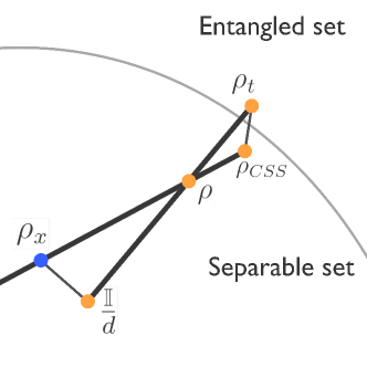
Figure 7: Schema of the method to get certification on lower bounds

In more detail, we start from a state $\rho$ we want to prove separable, and build a new state $\rho_{t}=(1+\epsilon)\rho-\epsilon\frac{\mathbb{I}}{d}$, where $\epsilon>0$ is an arbitrary small number such that $D_{\text{Tr}}(\rho_{t},\rho)$ is at least larger than the neural network’s precision. That new state $\rho_{t}$ will be further away from the fully mixed state. Then we use the neural network to obtain an approximately closest separable state to $\rho_{t}$, which we call $\rho_{\text{CSS}}$. Finally, we try to find a separable state $\rho_{x}=(1+\epsilon^{\prime})\rho-\epsilon^{\prime}\rho_{CSS}$ by scanning several values of $\epsilon^{\prime}$. We can use the condition $tr(\rho_{x}^{2})\leq\frac{1}{2^{N}-\alpha^{2}}$ with $\alpha^{2}=\frac{2^{N}}{\frac{17}{2}3^{N-3}+1}$ and $N$ the number of parties, from Ref. Barreiro et al. (2010a) to show that $\rho_{x}$ is fully separable. The condition $tr(\rho_{x}^{2})\leq\frac{1}{d-1}$ with $d$ the dimension of the Hilbert space from Ref. Barreiro et al. (2010b) can be used to show biseparability. If the condition is satisfied, the separability of $\rho$ follows from the convexity of the set of separable states.

References

- Horodecki et al. (2009) Ryszard Horodecki, Paweł Horodecki, Michał Horodecki, and Karol Horodecki, “Quantum entanglement,” Reviews of Modern Physics 81, 865–942 (2009), publisher: American Physical Society.
- Gühne and Toth (2009) Otfried Gühne and Geza Toth, “Entanglement detection,” Physics Reports 474, 1–75 (2009), arXiv: 0811.2803.
- Gurvits (2003) Leonid Gurvits, “Classical deterministic complexity of Edmonds’ Problem and quantum entanglement,” in Proceedings of the thirty-fifth annual ACM symposium on Theory of computing, STOC ’03 (Association for Computing Machinery, New York, NY, USA, 2003) pp. 10–19.
- Gharibian (2010) S. Gharibian, “Strong NP-hardness of the quantum separability problem,” Quantum Information and Computation 10, 343–360 (2010).
- Peres (1996) Asher Peres, “Separability Criterion for Density Matrices,” Physical Review Letters 77, 1413–1415 (1996), publisher: American Physical Society.
- Horodecki et al. (1996) Michał Horodecki, Paweł Horodecki, and Ryszard Horodecki, “Separability of mixed states: necessary and sufficient conditions,” Physics Letters A 223, 1–8 (1996).
- Horodecki et al. (1998) Michał Horodecki, Paweł Horodecki, and Ryszard Horodecki, “Mixed-State Entanglement and Distillation: Is there a “Bound” Entanglement in Nature?” Physical Review Letters 80, 5239–5242 (1998), publisher: American Physical Society.
- Navascués et al. (2009) Miguel Navascués, Masaki Owari, and Martin B. Plenio, “Complete Criterion for Separability Detection,” Physical Review Letters 103, 160404 (2009), publisher: American Physical Society.
- Barreiro et al. (2010a) Julio T. Barreiro, Philipp Schindler, Otfried Gühne, Thomas Monz, Michael Chwalla, Christian F. Roos, Markus Hennrich, and Rainer Blatt, “Experimental multiparticle entanglement dynamics induced by decoherence,” Nature Physics 6, 943–946 (2010a), bandiera_abtest: a Cg_type: Nature Research Journals Number: 12 Primary_atype: Research Publisher: Nature Publishing Group.
- Kampermann et al. (2012) Hermann Kampermann, Otfried Gühne, Colin Wilmott, and Dagmar Bruß, “Algorithm for characterizing stochastic local operations and classical communication classes of multiparticle entanglement,” Physical Review A 86, 032307 (2012), publisher: American Physical Society.
- Vedral et al. (1997) V. Vedral, M. B. Plenio, M. A. Rippin, and P. L. Knight, “Quantifying Entanglement,” Physical Review Letters 78, 2275–2279 (1997), publisher: American Physical Society.
- Pittenger and Rubin (2002) Arthur O. Pittenger and Morton H. Rubin, “Convexity and the separability problem of quantum mechanical density matrices,” Linear Algebra and its Applications 346, 47–71 (2002).
- Bertlmann et al. (2002a) R. A. Bertlmann, H. Narnhofer, and W. Thirring, “Geometric picture of entanglement and Bell inequalities,” Physical Review A 66, 032319 (2002a), publisher: American Physical Society.
- Pittenger and Rubin (2003) Arthur O. Pittenger and Morton H. Rubin, “Geometry of entanglement witnesses and local detection of entanglement,” Physical Review A 67, 012327 (2003), publisher: American Physical Society.
- Bertlmann et al. (2005a) Reinhold A. Bertlmann, Katharina Durstberger, Beatrix C. Hiesmayr, and Philipp Krammer, “Optimal entanglement witnesses for qubits and qutrits,” Physical Review A 72, 052331 (2005a), publisher: American Physical Society.
- Bertlmann and Krammer (2008) Reinhold A. Bertlmann and Philipp Krammer, “Geometric entanglement witnesses and bound entanglement,” Physical Review A 77, 024303 (2008), publisher: American Physical Society.
- Kim et al. (2010) Hungsoo Kim, Mi-Ra Hwang, Eylee Jung, and DaeKil Park, “Difficulties in analytic computation for relative entropy of entanglement,” Physical Review A 81, 052325 (2010), publisher: American Physical Society.
- Lewenstein and Sanpera (1998) Maciej Lewenstein and Anna Sanpera, “Separability and Entanglement of Composite Quantum Systems,” Physical Review Letters 80, 2261–2264 (1998), publisher: American Physical Society.
- Ishizaka (2002) Satoshi Ishizaka, “The reduction of the closest disentangled states,” Journal of Physics A: Mathematical and General 35, 8075–8081 (2002), publisher: IOP Publishing.
- Hayashi et al. (2008) Masahito Hayashi, Damian Markham, Mio Murao, Masaki Owari, and Shashank Virmani, “Entanglement of multiparty-stabilizer, symmetric, and antisymmetric states,” Physical Review A 77, 012104 (2008), publisher: American Physical Society.
- Hayashi et al. (2009) Masahito Hayashi, Damian Markham, Mio Murao, Masaki Owari, and Shashank Virmani, “The geometric measure of entanglement for a symmetric pure state with non-negative amplitudes,” Journal of Mathematical Physics 50, 122104 (2009), publisher: American Institute of Physics.
- Hübener et al. (2009) Robert Hübener, Matthias Kleinmann, Tzu-Chieh Wei, Carlos González-Guillén, and Otfried Gühne, “Geometric measure of entanglement for symmetric states,” Physical Review A 80, 032324 (2009), publisher: American Physical Society.
- Parashar and Rana (2011) Preeti Parashar and Swapan Rana, “Entanglement and discord of the superposition of Greenberger-Horne-Zeilinger states,” Physical Review A 83, 032301 (2011), publisher: American Physical Society.
- Carrington et al. (2015) M. E. Carrington, G. Kunstatter, J. Perron, and S. Plosker, “On the geometric measure of entanglement for pure states,” Journal of Physics A: Mathematical and Theoretical 48, 435302 (2015), publisher: IOP Publishing.
- Quesada and Sanpera (2014) Ruben Quesada and Anna Sanpera, “Best separable approximation of multipartite diagonal symmetric states,” Physical Review A 89, 052319 (2014), publisher: American Physical Society.
- Akulin et al. (2015) V. M. Akulin, G. A. Kabatiansky, and A. Mandilara, “Essentially entangled component of multipartite mixed quantum states, its properties, and an efficient algorithm for its extraction,” Physical Review A 92, 042322 (2015), publisher: American Physical Society.
- Rodriques et al. (2014) Samuel Rodriques, Nilanjana Datta, and Peter Love, “Bounding polynomial entanglement measures for mixed states,” Physical Review A 90, 012340 (2014), publisher: American Physical Society.
- Shang and Gühne (2018) Jiangwei Shang and Otfried Gühne, “Convex Optimization over Classes of Multiparticle Entanglement,” Physical Review Letters 120, 050506 (2018), publisher: American Physical Society.
- Wang (2017) Bingjie Wang, “Learning to Detect Entanglement,” arXiv:1709.03617 [quant-ph] (2017), arXiv: 1709.03617.
- Yosefpor et al. (2020) Mohammad Yosefpor, Mohammad Reza Mostaan, and Sadegh Raeisi, “Finding semi-optimal measurements for entanglement detection using autoencoder neural networks,” Quantum Science and Technology 5, 045006 (2020), publisher: IOP Publishing.
- Lu et al. (2018) Sirui Lu, Shilin Huang, Keren Li, Jun Li, Jianxin Chen, Dawei Lu, Zhengfeng Ji, Yi Shen, Duanlu Zhou, and Bei Zeng, “Separability-entanglement classifier via machine learning,” Physical Review A 98, 012315 (2018), publisher: American Physical Society.
- Gao et al. (2018) Jun Gao, Lu-Feng Qiao, Zhi-Qiang Jiao, Yue-Chi Ma, Cheng-Qiu Hu, Ruo-Jing Ren, Ai-Lin Yang, Hao Tang, Man-Hong Yung, and Xian-Min Jin, “Experimental Machine Learning of Quantum States,” Physical Review Letters 120, 240501 (2018), publisher: American Physical Society.
- Ma and Yung (2018) Yue-Chi Ma and Man-Hong Yung, “Transforming Bell’s inequalities into state classifiers with machine learning,” npj Quantum Information 4, 1–10 (2018), number: 1 Publisher: Nature Publishing Group.
- Gray et al. (2018) Johnnie Gray, Leonardo Banchi, Abolfazl Bayat, and Sougato Bose, “Machine-Learning-Assisted Many-Body Entanglement Measurement,” Physical Review Letters 121, 150503 (2018), publisher: American Physical Society.
- Yang et al. (2019) Mu Yang, Chang-liang Ren, Yue-chi Ma, Ya Xiao, Xiang-Jun Ye, Lu-Lu Song, Jin-Shi Xu, Man-Hong Yung, Chuan-Feng Li, and Guang-Can Guo, “Experimental Simultaneous Learning of Multiple Nonclassical Correlations,” Physical Review Letters 123, 190401 (2019), publisher: American Physical Society.
- Goes et al. (2021) Caio B. D. Goes, Askery Canabarro, Eduardo I. Duzzioni, and Thiago O. Maciel, “Automated machine learning can classify bound entangled states with tomograms,” Quantum Information Processing 20, 99 (2021).
- Ren and Chen (2019) Changliang Ren and Changbo Chen, “Steerability detection of an arbitrary two-qubit state via machine learning,” Physical Review A 100, 022314 (2019), publisher: American Physical Society.
- Harney et al. (2020) Cillian Harney, Stefano Pirandola, Alessandro Ferraro, and Mauro Paternostro, “Entanglement classification via neural network quantum states,” New Journal of Physics 22, 045001 (2020), publisher: IOP Publishing.
- Harney et al. (2021) Cillian Harney, Mauro Paternostro, and Stefano Pirandola, “Mixed state entanglement classification using artificial neural networks,” New Journal of Physics 23, 063033 (2021), publisher: IOP Publishing.
- Carleo and Troyer (2017) Giuseppe Carleo and Matthias Troyer, “Solving the quantum many-body problem with artificial neural networks,” Science 355, 602–606 (2017), publisher: American Association for the Advancement of Science Section: Research Articles.
- Melko et al. (2019) Roger G. Melko, Giuseppe Carleo, Juan Carrasquilla, and J. Ignacio Cirac, “Restricted Boltzmann machines in quantum physics,” Nature Physics 15, 887–892 (2019), bandiera_abtest: a Cg_type: Nature Research Journals Number: 9 Primary_atype: Reviews Publisher: Nature Publishing Group Subject_term: Information theory and computation;Quantum information;Quantum simulation;Theoretical physics Subject_term_id: information-theory-and-computation;quantum-information;quantum-simulation;theoretical-physics.
- Yoshioka and Hamazaki (2019) Nobuyuki Yoshioka and Ryusuke Hamazaki, “Constructing neural stationary states for open quantum many-body systems,” Physical Review B 99, 214306 (2019), publisher: American Physical Society.
- Hartmann and Carleo (2019) Michael J. Hartmann and Giuseppe Carleo, “Neural-Network Approach to Dissipative Quantum Many-Body Dynamics,” Physical Review Letters 122, 250502 (2019), publisher: American Physical Society.
- Nagy and Savona (2019) Alexandra Nagy and Vincenzo Savona, “Variational Quantum Monte Carlo Method with a Neural-Network Ansatz for Open Quantum Systems,” Physical Review Letters 122, 250501 (2019), publisher: American Physical Society.
- Vicentini et al. (2019) Filippo Vicentini, Alberto Biella, Nicolas Regnault, and Cristiano Ciuti, “Variational Neural-Network Ansatz for Steady States in Open Quantum Systems,” Physical Review Letters 122, 250503 (2019), publisher: American Physical Society.
- Goodfellow et al. (2016) Ian Goodfellow, Yoshua Bengio, and Aaron Courville, Deep Learning (MIT Press, 2016).
- Eisert et al. (2003) J. Eisert, K. Audenaert, and M. B. Plenio, “Remarks on entanglement measures and non-local state distinguishability,” Journal of Physics A: Mathematical and General 36, 5605–5615 (2003), publisher: IOP Publishing.
- Aaronson et al. (2013) Benjamin Aaronson, Rosario Lo Franco, Giuseppe Compagno, and Gerardo Adesso, “Hierarchy and dynamics of trace distance correlations,” New Journal of Physics 15, 093022 (2013), publisher: IOP Publishing.
- Paula et al. (2013) F. M. Paula, Thiago R. de Oliveira, and M. S. Sarandy, “Geometric quantum discord through the Schatten 1-norm,” Physical Review A 87, 064101 (2013), publisher: American Physical Society.
- Nakano et al. (2013) Takafumi Nakano, Marco Piani, and Gerardo Adesso, “Negativity of quantumness and its interpretations,” Physical Review A 88, 012117 (2013), publisher: American Physical Society.
- Modi et al. (2010) Kavan Modi, Tomasz Paterek, Wonmin Son, Vlatko Vedral, and Mark Williamson, “Unified View of Quantum and Classical Correlations,” Physical Review Letters 104, 080501 (2010), publisher: American Physical Society.
- Bellomo et al. (2012) Bruno Bellomo, Gian Luca Giorgi, Fernando Galve, Rosario Lo Franco, Giuseppe Compagno, and Roberta Zambrini, “Unified view of correlations using the square-norm distance,” Physical Review A 85, 032104 (2012), publisher: American Physical Society.
- Vedral and Plenio (1998) V. Vedral and M. B. Plenio, “Entanglement measures and purification procedures,” Physical Review A 57, 1619–1633 (1998), publisher: American Physical Society.
- Witte and Trucks (1999) C. Witte and M. Trucks, “A new entanglement measure induced by the Hilbert–Schmidt norm,” Physics Letters A 257, 14–20 (1999).
- Krammer (2009) Philipp Krammer, “Characterizing entanglement with geometric entanglement witnesses,” Journal of Physics A: Mathematical and Theoretical 42, 065305 (2009), publisher: IOP Publishing.
- Vidal and Tarrach (1999) Guifré Vidal and Rolf Tarrach, “Robustness of entanglement,” Physical Review A 59, 141–155 (1999), publisher: American Physical Society.
- Zyczkowski and Bengtsson (2006) Karol Zyczkowski and Ingemar Bengtsson, “An Introduction to Quantum Entanglement: a Geometric Approach,” arXiv:quant-ph/0606228 (2006), arXiv: quant-ph/0606228.
- Kriváchy et al. (2020) Tamás Kriváchy, Yu Cai, Daniel Cavalcanti, Arash Tavakoli, Nicolas Gisin, and Nicolas Brunner, “A neural network oracle for quantum nonlocality problems in networks,” npj Quantum Information 6, 1–7 (2020), number: 1 Publisher: Nature Publishing Group.
- Horodecki et al. (2000) Paweł Horodecki, Maciej Lewenstein, Guifré Vidal, and Ignacio Cirac, “Operational criterion and constructive checks for the separability of low-rank density matrices,” Physical Review A 62, 032310 (2000), publisher: American Physical Society.
- Witte and Trucks (1999) Paweł Horodecki, Michał Horodecki, and Ryszard Horodecki, “Bound Entanglement Can Be Activated,” Physical Review Letters 82, 1056–1059 (1999), publisher: American Physical Society.
- Mintert et al. (2005) Florian Mintert, André R. R. Carvalho, Marek Kuś, and Andreas Buchleitner, “Measures and dynamics of entangled states,” Physics Reports 415, 207–259 (2005).
- Dür and Cirac (2000) W. Dür and J. I. Cirac, “Classification of multiqubit mixed states: Separability and distillability properties,” Physical Review A 61, 042314 (2000), publisher: American Physical Society.
- Chen and Jiang (2020) Xiao-yu Chen and Li-zhen Jiang, “Noise tolerance of Dicke states,” Physical Review A 101, 012308 (2020), publisher: American Physical Society.
- Szalay (2011) Szilárd Szalay, “Separability criteria for mixed three-qubit states,” Physical Review A 83, 062337 (2011), publisher: American Physical Society.
- Gühne and Seevinck (2010) Otfried Gühne and Michael Seevinck, “Separability criteria for genuine multiparticle entanglement,” New Journal of Physics 12, 053002 (2010), publisher: IOP Publishing.
- Jungnitsch et al. (2011) Bastian Jungnitsch, Tobias Moroder, and Otfried Gühne, “Taming Multiparticle Entanglement,” Physical Review Letters 106, 190502 (2011), publisher: American Physical Society.
- Fazel et al. (2001) M. Fazel, H. Hindi, and S.P. Boyd, “A rank minimization heuristic with application to minimum order system approximation,” in Proceedings of the 2001 American Control Conference. (Cat. No.01CH37148) (IEEE, 2001) p. 4734–4739 vol.6.
- Rana (2013) Swapan Rana, “Negative eigenvalues of partial transposition of arbitrary bipartite states,” Physical Review A 87, 054301 (2013), publisher: American Physical Society.
- Johnston and Kribs (2010) Nathaniel Johnston and David W. Kribs, “A family of norms with applications in quantum information theory,” Journal of Mathematical Physics 51, 082202 (2010), publisher: American Institute of Physics.
- Barreiro et al. (2010b) Leonid Gurvits and Howard Barnum, “Largest separable balls around the maximally mixed bipartite quantum state,” Phys. Rev. A 66, 062311 (2002).