Power of the Crowd

Abstract

Consider a Galton Watson tree of height $m$: each leaf has one of $k$ opinions or not. In other words, for $i\in\{1,\dots,k\}$, $x$ at generation $m$ thinks $i$ with probability $\mathbf{p}_{i}$ and nothing with probability $\mathbf{p}_{0}$. Moreover the opinions are independently distributed for each leaf.
Opinions spread along the tree based on a specific rule: the majority wins! In this paper, we study the asymptotic behavior of the distribution of the opinion of the root when $m\to\infty$.

1 Introduction

First let us recall the definition of a Galton Watson tree (GW) and give a few notations. Assume that $N$ is a $\mathbb{N}$-valued random variable following a distribution $q$: $\mathbb{P}(N=i)=q_{i}$ for $i\in\mathbb{N}$. In order to have a meaningful probabilistic setting, we assume that $q_{0}+q_{1}=0$ (Bötcher case).
Let $\phi$ be the root of the tree and $N_{\phi}$ an independent copy of $N$. Then, we draw $N_{\phi}$ children of $\phi$: these individuals are the first generation. In the following we write $N$ for $N_{\phi}$ for typographical simplicity. At the $m$-th generation, for each individual $x$ we pick $N_{x}$ an independent copy of $N$ where $N_{x}$ is the number of children of $x$ and so on. The set $\mathbb{T}$, consisting of the root and its descendants, forms a GW of offspring distribution $q$.
We denote by $|x|$ the generation of $x$ and for $m\in\mathbb{N}$, $\mathbb{T}_{m}=\{x\in\mathbb{T},|x|\leq m\}$ the GW cut at height $m$ and the leaves of $\mathbb{T}_{m}$ are the elements of $\mathbb{T}_{m}\backslash\mathbb{T}_{m-1}$.
Here we want to represent the propagation of an opinion in a population represented by a GW of height $m$. More precisely consider the set of probability vectors $\mathscr{P}_{k}$ defined by

$$\mathscr{P}_{k}:=\left\{\mathbf{p}=(\mathbf{p}_{0},\dots,\mathbf{p}_{k})\in(\mathbb{R}_{+})^{k+1}:\sum_{i=0}^{k}\mathbf{p}_{i}=1\ \ \text{and}\ \ \mathbf{p}_{0}<1\right\}\subset\mathbb{R}^{k+1},$$ (1.1)

and fix $\mathbf{p}\in\mathscr{P}_{k}$. Each node of $\mathbb{T}_{m}$ has the opinion $\{1,\dots,k\}$ according to the following rules:

• Independently of the others, each leaf has an opinion according to $\mathbf{p}$:

  $$\mathbb{P}(\mbox{leaf thinks $i$})=\mathbf{p}_{i}\ \ \ \text{and}\ \ \ \mathbb{P}(\mbox{leaf is undecided})=\mathbf{p}_{0}.$$

• The opinions spread to nodes at generation $m-1$ this way (see Figure 1):

  1. the undecided children have no influence, except when the children are all undecided, in that case their ancestor has no opinion;

  2. if a relative majority of the children shares the same opinion, the ancestor thinks the same;

  3. if several opinions are equally represented and the others are less, then the ancestor is undecided.

• We repeat this step for level $m-2$ and so on (see Figure 2).

Figure 1: The rules

Figure 2: An example

As claimed, we want to determine the asymptotic behavior of the distribution $\mathbf{p}(m)$ of the state at the root of $\mathbb{T}_{m}$ when $m$ goes to infinity:

$$\forall\,1\leq i\leq k,\ \mathbb{P}(\mbox{root thinks }i)=\mathbf{p}_{i}(m)\ \ \ \text{and}\ \ \ \mathbb{P}(\mbox{root is undecided})=\mathbf{p}_{0}(m).$$

The children $\phi i$ of the root $\phi$ of $\mathbb{T}_{m}$, with $i\in\{1,\dots,N\}$, are root nodes of $N$ independent GW of height $m-1$. Then the distribution $\mathbf{p}(m)=\left(\mathbf{p}_{0}(m),\mathbf{p}_{1}(m),\dots,\mathbf{p}_{k}(m)\right)$ of the state of $\phi$ is completely determined by the distribution $\mathbf{p}(m-1)$ of the independent states of the $\phi i$, $i\in\{1,\dots,N\}$. Let $H:\mathscr{P}_{k}\rightarrow\mathscr{P}_{k}$ be the function satisfying $\mathbf{p}(m)=H(\mathbf{p}(m-1))$, cf. (2.2). An obvious reasoning by induction implies $H^{m}(\mathbf{p})=\mathbf{p}(m)\in\mathscr{P}_{k}$. As a result, our problem consists in studying the orbits of $H$ in $\mathscr{P}_{k}$.

The case of the binary tree is completely studied in [2] and our paper can be seen as its natural generalization. Note that the relative majority is not the only possible extension of [2]: in [5], the authors replaced (R2) and (R3) by the following rules

1. if two children have different opinions, the ancestor is undecided;

2. if all the children share the same opinion, the ancestor has it.

We highlight the major differences between the results of [2, 5] and ours after the statement of our main results.

In what follows, we assume without loss of generality that $\mathbf{p}_{1}>0$ and $\mathbf{p}_{1}\geq\dots\geq\mathbf{p}_{k}$. It then holds $H_{1}(\mathbf{p})\geq\dots\geq H_{k}(\mathbf{p})$ and, if there exists $i\in\{1,\dots,k-1\}$ such that $\mathbf{p}_{i+1}=\dots=\mathbf{p}_{k}=0$, then $H_{i+1}(\mathbf{p})=\dots=H_{k}(\mathbf{p})=0$ (see remark 2.1).

It is hence sufficient to study the behavior of $H$ when acting on $\mathscr{P}_{i}$. If there exists $i\in\{1,\dots,k-1\}$ such that $\mathbf{p}_{1}=\dots=\mathbf{p}_{i}>\mathbf{p}_{i+1}\geq\dots\geq\mathbf{p}_{k}>0$, then ${i+1},\dots,k$ are called minor opinions and otherwise, i.e. if $\mathbf{p}_{1}=\mathbf{p}_{2}=\dots=\mathbf{p}_{k}>0$, we say that we are in the uniform case.

In Section 2, we prove that the major opinions do not vanish when $m\to\infty$, contrary to the minor opinions, and we state in Proposition 2.8 a sufficient criterion to reduce the analysis to the uniform case. The biggest advantage of the uniform case is to study the fixed points of a function defined on (a subset of) $\mathbb{R}$ instead of those of a function on $\mathscr{P}_{k}$. It naturally follows that if there is only one major opinion, regardless of the law of reproduction of $N$, this opinion spreads a.s. to the root asymptotically.
Although we have stated a very general problem, our main results below are available in more restrictive cases: we only consider $n$-ary trees for $n\geq 2$ or GW trees supported in $2\mathbb{N}+1$ and two major opinions. This includes in particular a binary (“for-against") referendum, an election with two candidates. In the case of a $n$-ary tree for $n\geq 2$, we obtain the following

Theorem 1.1

For every $k\geq 2$ and $\mathbf{p}\in\mathscr{P}_{k}$ such that $\mathbf{p}_{1}=\mathbf{p}_{2}>\mathbf{p}_{3}\geq\dots\geq\mathbf{p}_{k}$ and $\mathbf{p}_{1}<\frac{1}{2}$, $\mathbf{p}(m)$ converges to $\left(\alpha_{n},\frac{1-\alpha_{n}}{2},\frac{1-\alpha_{n}}{2},0_{k-2}\right)$ when $m\to\infty$, where $\alpha_{n}$ is the unique fixed point in $(0,1)$ of the function

$$f_{n}:t\in[0,1]\longmapsto\sum_{k,0\leq 2k\leq n}\binom{n}{2k}\binom{2k}{k}\left(\frac{1-t}{2}\right)^{2k}t^{n-2k}\in[0,1].$$

Moreover, the above convergence remains true when $\mathbf{p}_{1}=\mathbf{p}_{2}=\frac{1}{2}$ and $n$ is even, whereas $\mathbf{p}(m)=(0,\frac{1}{2},\frac{1}{2},0_{k-2})$ for every $m\geq 0$ when $\mathbf{p}_{1}=\mathbf{p}_{2}=\frac{1}{2}$ and $n$ is odd.

The following result on the GW trees is “just" a corollary as it needs to add a tricky argument to the proof of Theorem 1.1 in the odd case.

Corollary 1.2

Taking a GW tree whose support is included in $2\mathbb{N}+1$ and such that $\mathbb{E}[N^{2}]<\infty$, the result of Theorem 1.1 for odd $n$ remains true, replacing $\alpha_{n}$ by $\alpha$, the unique fixed point in $(0,1)$ of

$$f:t\in[0,1]\longmapsto\sum_{n\geq 1}q_{2n+1}f_{2n+1}(t).$$

As claimed, we make a brief list of the differences in [2] and [5].
In [2], one can see that for $n=2$, the result of Theorem 1.1 is still true for any number of major opinions and the limit is explicit, in other words for all $i\geq 2$ and $\mathbf{p}_{1}=\cdots=\mathbf{p}_{i}>\mathbf{p}_{i+1}\geq\dots\geq\mathbf{p}_{k}$, $\mathbf{p}(m)$ converges to $\left(\frac{i-1}{2i-1},\frac{1}{2i-1},\dots,\frac{1}{2i-1},0_{k-i}\right)$.
With the rules explained in [5], the function studied in the uniform case with a $n$-ary tree and $i$ major opinions is the following:

$$g_{n}:t\in[0,\nicefrac{{1}}{{i}}]\longmapsto(1-(i-1)t)^{n}-(1-it)^{n}$$

and one can see this as the probability that the first opinion spreads. This function admits a unique fixed point $\bar{x}$ in $(0,\nicefrac{{1}}{{i}}]$ and the authors show that for $n\in\{3,4,5\}$, $\mathbf{p}(m)$ converges to $(1-i\bar{x},\bar{x},\dots,\bar{x},0_{k-i})$. For $n\geq 6$, stranger things happen: for instance for $n=6$, $\bar{x}$ is a repelling fixed point of $g_{n}$ and, if $i=2$, the authors show that there is a unique attracting orbit of prime period 2. Moreover, numerical simulations suggest the existence of a unique attracting orbit for every $n$ and $i$.

Let us come back to the organization of the paper: in Section 3, we give the proof of Theorem 1.1 and Corollary 1.2. If the support of the GW tree is a subset of $2\mathbb{N}$, we have just succeeded to prove that if there is convergence, it does to $\left(\alpha,\frac{1-\alpha}{2},\frac{1-\alpha}{2},0_{k-2}\right)$, where $\alpha$ is the unique fixed point in $[0,1)$ of

$$f:t\in[0,1]\longmapsto\sum_{n\geq 1}q_{2n}f_{2n}(t).$$

We have the attractivity but do not succeed to prove that we have convergence for all $\mathbf{p}\in\mathscr{P}_{k}$. In this section, we also provide bounds for the values of the fixed points $\alpha_{n}$ of the functions $f_{n}$.
The general case seems to be unreachable for the moment, we just have proved the existence of a non-repulsive fixed point, not even its uniqueness. Nevertheless, we give an example where everything works, the geometric law, in Section 4.
Finally, in Section 5 we make some remarks and give open questions and Section 6 is an Appendix.

2 Reduction to the Uniform case

As stated in the introduction, the aim of the present paper is the study of a particular type of dynamical systems: more precisely, given the function $H:\mathscr{P}_{k}\rightarrow\mathscr{P}_{k}$ defined below (see (2.2)), we are interested in the behavior of the orbits $H^{\ell}(x)$ of the elements $x\in\mathscr{P}_{k}$ (see (1.1)) when $\ell$ goes to infinity. In this section we give sufficient conditions to reduce the problem to a subfamily of functions $H$ corresponding to the uniform case, namely the functions $h_{k}$ defined below (see (2.4)).

First, we need to specify the function $H$. Summing on the number of children of a “typical” node and on the number of children with a neutral opinion, the probability that, for $i=1,\dots,k$, the $i$-th opinion spreads to their parent is equal to

$$\sum_{n\geq 2}q_{n}\sum_{m_{0}=0}^{n-1}\binom{n}{m_{0}}\mathbf{p}_{0}^{m_{0}}\sum_{S^{i}_{n-m_{0}}}\binom{n-m_{0}}{m_{1},m_{2},\dots,m_{k}}\prod_{j=1}^{k}\mathbf{p}_{j}^{m_{j}}\,,$$ (2.1)

where $S^{i}_{n}=\{(m_{1},\dots,m_{k})\in\mathbb{N}^{k},\forall j\neq i,m_{j}<m_{i}\in\mathbb{N},\sum_{j=1}^{k}m_{j}=n\}$ and $\binom{n}{m_{1},m_{2},\dots,m_{k}}$ is the multinomial coefficient. Our problem then requires to study the fixed points in $\mathscr{P}_{k}$ of the function $H:\mathscr{P}_{k}\rightarrow\mathbb{R}^{k+1}$ defined by:

$$H_{i}(\mathbf{p}_{0},\dots,\mathbf{p}_{k})=\left\{\begin{array}[]{ccc}\sum\limits_{n\geq 2}q_{n}\sum\limits_{m_{0}=0}^{n-1}\binom{n}{m_{0}}\mathbf{p}_{0}^{m_{0}}\sum\limits_{S^{i}_{n-m_{0}}}\binom{n-m_{0}}{m_{1},m_{2},\dots,m_{k}}\prod\limits_{j=1}^{k}\mathbf{p}_{j}^{m_{j}}&\mbox{when $i\neq 0$,}\\ 1-\sum\limits_{j=1}^{k}H_{j}(\mathbf{p}_{0},\dots,\mathbf{p}_{k}).&\mbox{when $i=0$.}\end{array}\right.$$ (2.2)

Remark 2.1

Note that $\mathscr{P}_{k}$ is stable by $H$ and that, for $\mathbf{p}\in\mathscr{P}_{k}$, we can assume without loss of generality that $\mathbf{p}_{1}\geq\dots\geq\mathbf{p}_{k}$ (which implies $\mathbf{p}_{1}>0$ by definition of $\mathscr{P}_{k}$, see (1.1)).
In this case, it holds $H_{1}(\mathbf{p})\geq\dots\geq H_{k}(\mathbf{p})$ as well as, for every $i\in\{1,\dots,k\}$: $H_{i}(\mathbf{p})>0$ if, and only if, $\mathbf{p}_{i}>0$.
In particular, if there exists $i\in\{1,\dots,k-1\}$ such that $\mathbf{p}_{i+1}=\dots=\mathbf{p}_{k}=0$, then $H_{i+1}(\mathbf{p})=\dots=H_{k}(\mathbf{p})=0$ and it is thus sufficient to study $H:\mathscr{P}_{i}\subset\mathbb{R}^{i+1}\to\mathscr{P}_{i}$.

In what follows we denote, for $k\in\mathbb{N}$,

$$\mathscr{Q}_{k}:=\{\mathbf{p}\in\mathscr{P}_{k}\,,\ \mathbf{p}_{1}\geq\dots\geq\mathbf{p}_{k}\}$$ (2.3)

and according to the previous remark we only need to consider the action of the function $H$ on $\mathscr{Q}_{k}$.

In the uniform case, i.e. when $\mathbf{p}_{1}=\dots=\mathbf{p}_{k}\in(0,\frac{1}{k}]$, one has simply $H(1-k\mathbf{p}_{1},\mathbf{p}_{1},\dots,\mathbf{p}_{1})=(1-kh_{k}(\mathbf{p}_{1}),h_{k}(\mathbf{p}_{1}),\dots,h_{k}(\mathbf{p}_{1}))$, where $h_{k}$ is the real function defined on $[0,\frac{1}{k}]$ by

$$h_{k}(x)=\sum_{n\geq 2}q_{n}\sum_{m_{0}=0}^{n-1}\binom{n}{m_{0}}(1-kx)^{m_{0}}\sum_{S^{1}_{n-m_{0}}}\binom{n-m_{0}}{m_{1},m_{2},\dots,m_{k}}x^{n-m_{0}}\in\left[0,\frac{1}{k}\right]\,.$$ (2.4)

The study of the fixed points in $\mathscr{Q}_{k}$ of $H$ in the uniform case is thus reduced to the study of the fixed points in $(0,\frac{1}{k}]$ of $h_{k}$. Note also here that $0$ is a fixed point of $h_{k}$ which is repulsive, since

$$h^{\prime}_{k}(0)=\sum_{n\geq 2}q_{n}\binom{n}{n-1}\sum_{S^{1}_{1}}\binom{1}{m_{1},m_{2},\dots,m_{k}}=\sum_{n\geq 2}n\,q_{n}=\mathbb{E}[N]\geq 2\,.$$

Let us also recall that the generating function $G$ of $N$ is defined by

$$\forall s\in[-1,1],\,G(s)=\mathbb{E}\left[s^{N}\right]=\sum_{n\geq 0}s^{n}\mathbb{P}(N=n)=\sum_{n\geq 0}s^{n}q_{n}.$$ (2.5)

On $(-1,1)$, $G$ is $\mathscr{C}^{\infty}$ and:

$$\forall k\in\mathbb{N},\,G^{(k)}(s)=\mathbb{E}[N(N-1)\dots(N-k+1)s^{N-k}]\,,$$ (2.6)

implying that

$$\forall k\in\mathbb{N},\,G^{(k)}(1^{-})=\mathbb{E}[N(N-1)\dots(N-k+1)]\quad\mbox{ and }\quad G^{(k)}(0)=k!\,q_{k}.$$ (2.7)

In particular, we have here $G(0)=\mathbb{P}(N=0)=0$, $G^{\prime}(0)=\mathbb{P}(N=1)=0$, and $G^{\prime}(1^{-})=\mathbb{E}[N]\geq 2$.

Lemma 2.2

Assume that $\mathbf{p}\in\mathscr{Q}_{k}$ and that $G^{(2)}(1)$ is finite. Then, there exists $\eta>0$ such that

$$\forall m\in\mathbb{N},\ \ \mathbf{p}_{1}(m)\geq\beta:=\min\{\eta^{\mathfrak{a}}q_{\mathfrak{a}},\mathbf{p}_{1}\}\,,$$

where $\mathfrak{a}:=\inf\{n\geq 2,q_{n}\neq 0\}$.

Proof. For $\mathbf{p}\in\mathscr{Q}_{k}$, we have $\mathbf{p}_{1}>0$, $\mathbf{p}_{1}\geq\cdots\geq\mathbf{p}_{k}$, and $\mathbf{p}_{0}=1-\sum_{i=1}^{k}\mathbf{p}_{i}$. We get

$$H_{1}(\mathbf{p})>\sum_{n\geq 2}q_{n}\binom{n}{n-1}\mathbf{p}_{0}^{n-1}\sum_{S^{1}_{1}}\binom{1}{m_{1},m_{2},\dots,m_{k}}\prod_{j=1}^{k}\mathbf{p}_{j}^{m_{j}} = \sum_{n\geq 2}q_{n}n\mathbf{p}_{1}\mathbf{p}_{0}^{n-1}$$ (2.8)

$$= \mathbf{p}_{1}G^{\prime}\left(1-\sum_{i=1}^{k}\mathbf{p}_{i}\right).$$

Since $G^{(2)}(1)=\mathbb{E}[N(N-1)]\in\mathbb{R}_{+}^{*}$, one can write

$$G^{\prime}(1-t)=G^{\prime}(1)-tG^{(2)}(1)+\varepsilon(t),$$

where $\frac{\varepsilon(t)}{t}\underset{t\rightarrow 0}{\longrightarrow}0$.

As a result, there exists $0<\eta^{\prime}<\nicefrac{{G^{\prime}(1)}}{{3G^{(2)}(1)}}$ such that $|\varepsilon(t)|\leq\frac{tG^{(2)}(1)}{2}$ when $0\leq t\leq\eta^{\prime}$. Then, for $0\leq x\leq\eta:=\frac{\eta^{\prime}}{k}$ and $0\leq y\leq(k-1)x$,

$$xG^{\prime}(1-x-y) \geq x\left(G^{\prime}(1)-(x+y)G^{(2)}(1)-(x+y)\frac{G^{(2)}(1)}{2}\right)=x\left(G^{\prime}(1)-3(x+y)\frac{G^{(2)}(1)}{2}\right)$$

$$\geq x\left(G^{\prime}(1)-\frac{G^{\prime}(1)}{2}\right)=x\frac{G^{\prime}(1)}{2}\geq x,$$

where the last inequality follows from $G^{\prime}(1)=\mathbb{E}[N]\geq 2$.

Thus, according to (2.8), $H_{1}(\mathbf{p})\geq\mathbf{p}_{1}$ when $\mathbf{p}_{1}\leq\eta$. In addition, when $\mathbf{p}_{1}>\eta$ :

$$H_{1}(\mathbf{p})\geq\sum_{n\geq\mathfrak{a}}q_{n}\binom{n}{n-\mathfrak{a}}\mathbf{p}_{0}^{n-\mathfrak{a}}\mathbf{p}_{1}^{\mathfrak{a}}=\frac{\mathbf{p}_{1}^{\mathfrak{a}}}{\mathfrak{a}!}G^{(\mathfrak{a})}(\mathbf{p}_{0})\geq\frac{\mathbf{p}_{1}^{\mathfrak{a}}}{\mathfrak{a}!}G^{(\mathfrak{a})}(0)\geq\eta^{\mathfrak{a}}q_{\mathfrak{a}}>0.$$

An obvious recurrence gives the claimed result.   $\quad\square$

Remark 2.3

Applying the relation (2.8) to a fixed point $(\mathbf{p}_{0},\mathbf{p}_{1},\dots,\mathbf{p}_{k})\in\mathscr{Q}_{k}$ of $H$ we get

$$\mathbf{p}_{1}=H_{1}(\mathbf{p})>\sum_{n\geq 2}q_{n}\binom{n}{n-1}\mathbf{p}_{0}^{n-1}\mathbf{p}_{1}=\mathbf{p}_{1}G^{\prime}(\mathbf{p}_{0})\,,$$

then, since $\mathbf{p}_{1}>0$,

$$G^{\prime}(\mathbf{p}_{0})<1.$$

The following elementary lemma ensures the validity of further results using the differentiability of $H$ on $\mathscr{P}_{k}$.

Lemma 2.4

Suppose that $G^{\prime}(1)$ is finite. Let $\mathscr{J}_{k}:=\left\{\mathbf{p}=(\mathbf{p}_{0},\dots,\mathbf{p}_{k})\in(\mathbb{R}_{+})^{k+1}:\sum_{i=0}^{k}\mathbf{p}_{i}\leq 1\right\}$ and still denote by $H_{i}$ the functions defined by (2.2) on $\mathscr{J}_{k}$ for $1\leq i\leq k$. Then, these functions are of class $\mathscr{C}^{1}$ on $\mathscr{J}_{k}$.

Proof. Note first that by definition, for every $1\leq i\leq k$ and $\mathbf{p}\in\mathscr{J}_{k}$, $H_{i}(\mathbf{p})$ writes:

$$H_{i}(\mathbf{p}):=\sum\limits_{n\geq 2}q_{n}H_{i,n}(\mathbf{p}):=\sum\limits_{n\geq 2}q_{n}\sum_{m\in{\mathbb{N}}^{k+1},|m|=n}a_{n,m}\mathbf{p}^{m},$$

where $a_{n,m}\in\mathbb{R}^{+}$ and, for every $m=(m_{0},\dots,m_{k})\in{\mathbb{N}}^{k+1}$, $|m|:=\sum_{i=0}^{k}m_{i}$ and $\mathbf{p}^{m}:=\prod_{i=0}^{k}\mathbf{p}_{i}^{m_{i}}$. More precisely, for every $n\geq 2$ and $m\in{\mathbb{N}}^{k+1}$ satisfying $|m|=n$,

$$0\leq a_{n,m}\leq\binom{n}{m}\quad\text{and hence}\quad H_{i,n}(\mathbf{p})\leq\!\!\!\!\sum_{m\in{\mathbb{N}}^{k+1},|m|=n}\binom{n}{m}\mathbf{p}^{m}=(\mathbf{p}_{0}+\cdots+\mathbf{p}_{k})^{n}\leq\ 1.$$

It follows that, for every $1\leq i\leq k$, $H_{i}$ is continuous on $\mathscr{J}_{k}$ and satisfies

$$\forall\mathbf{p}\in\mathscr{J}_{k},\ \ \ H_{i}(\mathbf{p})=\sum\limits_{n\geq 2}q_{n}H_{i,n}(\mathbf{p})\leq\sum\limits_{n\geq 2}q_{n}(\mathbf{p}_{0}+\cdots+\mathbf{p}_{k})^{n}=G(\mathbf{p}_{0}+\cdots+\mathbf{p}_{k}).$$

Moreover, for every $\ell\in\{0,\dots,k\}$, $\mathbf{p}\in\mathscr{J}_{k}$, and $n\geq 2$:

$$0\leq\frac{\partial H_{i,n}}{\partial\mathbf{p}_{\ell}}(\mathbf{p})\leq\frac{\partial(\mathbf{p}_{0}+\cdots+\mathbf{p}_{k})^{n}}{\partial\mathbf{p}_{\ell}}=n(\mathbf{p}_{0}+\cdots+\mathbf{p}_{k})^{n-1}\leq n.$$

This implies the claimed result, since $G^{\prime}(1)=\sum\limits_{n\geq 2}nq_{n}$ is finite.   $\quad\square$

The following lemma ensures that the minor opinions can not spread to the root asymptotically:

Lemma 2.5

Assume that $G^{(2)}(1)$ is finite. In the (non uniform) case with $i<k\in\mathbb{N}^{*}$ and $\mathbf{p}\in\mathscr{Q}_{k}$ such that $\mathbf{p}_{1}=\dots=\mathbf{p}_{i}>\mathbf{p}_{i+1}\geq\dots\geq\mathbf{p}_{k}\geq 0$, it holds $\mathbf{p}_{j}(m)\underset{m\rightarrow\infty}{\rightarrow}0$ for every $j\in\{i+1,\dots,k\}$.

Proof. Note that we just have to prove that $\lim\limits_{n\to\infty}\mathbf{p}_{i+1}(n)=0$ when $\mathbf{p}_{i+1}>0$. In this case, writing $w_{n}=\frac{\mathbf{p}_{i+1}(n)}{\mathbf{p}_{1}(n)}>0$, we can easily see that for every $n\geq 0$, $w_{n+1}=w_{n}u_{n}$, where:

$$u_{n}:=\frac{\displaystyle\sum_{z\geq 2}q_{z}\sum_{m_{0}=0}^{z-1}\binom{z}{m_{0}}\mathbf{p}_{0}^{m_{0}}(n)\sum_{S_{z-m_{0}}^{1}}\binom{z-m_{0}}{m_{1},m_{2},\dots,m_{k}}\mathbf{p}_{i+1}^{m_{1}-1}(n)\mathbf{p}_{1}^{m_{i+1}}(n)\prod_{j=2,j\neq i+1}^{k}\mathbf{p}_{j}^{m_{j}}(n)}{\displaystyle\sum_{z\geq 2}q_{z}\sum_{m_{0}=0}^{z-1}\binom{z}{m_{0}}\mathbf{p}_{0}^{m_{0}}(n)\sum_{S_{z-m_{0}}^{1}}\binom{z-m_{0}}{m_{1},m_{2},\dots,m_{k}}\mathbf{p}_{1}^{m_{1}-1}(n)\mathbf{p}_{i+1}^{m_{i+1}}(n)\prod_{j=2,j\neq i+1}^{k}\mathbf{p}_{j}^{m_{j}}(n)}.$$

For every $(m_{1},\dots,m_{k})\in S^{1}_{z-m_{0}}$, since $\mathbf{p}_{1}>\mathbf{p}_{i+1}>0$, we have that $\mathbf{p}_{i+1}^{m_{1}-1}(n)\mathbf{p}_{1}^{m_{i+1}}(n)<\mathbf{p}_{1}^{m_{1}-1}(n)\mathbf{p}_{i+1}^{m_{i+1}}(n)$ when $m_{i+1}<m_{1}-1$, implying that $0<w_{n+1}<w_{n}$. Thus, $(w_{n})$ is a positive decreasing sequence, and consequently converges to some $\ell\geq 0$. Since $w_{0}<1$, note that $\ell<1$.
By compacity, there exists moreover a subsequence ${n_{m}}$ such that $\lim\limits_{m\to\infty}\mathbf{p}_{j}(n_{m})=a_{j}$ for every $j=0,\dots,k$. From Lemma 2.2, we have $a_{1}>0$. Now, assume that $a_{i+1}>0$. Since $\ell<1$, we have $a_{1}>a_{i+1}>0$ and, using the definition of $u_{n}$:

$$\lim_{m\rightarrow\infty}u_{n_{m}}=\frac{\displaystyle\sum_{z\geq 2}q_{z}\sum_{m_{0}=0}^{z-1}\binom{z}{m_{0}}a_{0}^{m_{0}}\sum_{S^{1}_{z-m_{0}}}\binom{z-m_{0}}{m_{1},m_{2},\dots,m_{k}}a_{i+1}^{m_{1}-1}a_{1}^{m_{i+1}}\prod_{j=2,j\neq i+1}^{k}a_{j}^{m_{j}}}{\displaystyle\sum_{z\geq 2}q_{z}\sum_{m_{0}=0}^{z-1}\binom{z}{m_{0}}a_{0}^{m_{0}}\sum_{S^{1}_{z-m_{0}}}\binom{z-m_{0}}{m_{1},m_{2},\dots,m_{k}}a_{1}^{m_{1}-1}a_{i+1}^{m_{i+1}}\prod_{j=2,j\neq i+1}^{k}a_{j}^{m_{j}}}=\ell^{\prime}<1.$$

This permits us to easily conclude:

$$\ell=\lim_{m\rightarrow\infty}w_{n_{m}+1}=\lim_{m\rightarrow\infty}w_{n_{m}}u_{n_{m}}=\ell\ell^{\prime}<\ell\,,$$

which is a contradiction. Then $a_{i+1}=0$ and consequently $\mathbf{p}_{i+1}(n)\underset{n\rightarrow\infty}{\rightarrow}0$.   $\quad\square$

Remark 2.6

Actually, for every $j\in\{i+1,\dots,k\}$, the convergence $\mathbf{p}_{j}(m)\underset{m\rightarrow\infty}{\rightarrow}0$ is exponential, i.e.

$$\exists\,a\in(0,1)\,,\ \exists\,C>0\,,\ \forall\,m\in\mathbb{N}\,:\ \ 0\leq\mathbf{p}_{k}(m)\leq\dots\leq\mathbf{p}_{i+1}(m)\leq Ca^{m}\,.$$ (2.9)

Note that to prove (2.9), it suffices to show that $\limsup\limits_{n\to\infty}u_{n}<1$, where $(u_{n})_{n\geq 0}$ is the positive sequence introduced in the preceding proof. But since $\mathbf{p}_{i+1}(m)\underset{m\rightarrow\infty}{\rightarrow}0$, there exists a sequence $(\varepsilon_{n})_{n\geq 0}$ converging to $0$ such that:

$$u_{n} =\frac{\displaystyle\sum_{z\geq 2}q_{z}\binom{z}{z-1}\mathbf{p}_{0}^{z-1}(n)\ +\ \varepsilon_{n}}{\displaystyle\sum_{z\geq 2}q_{z}\sum_{m_{0}=0}^{z-1}\binom{z}{m_{0}}\mathbf{p}_{0}^{m_{0}}(n)\sum_{S_{z-m_{0}}^{1}}\binom{z-m_{0}}{m_{1},m_{2},\dots,m_{k}}\mathbf{p}_{1}^{m_{1}-1}(n)\mathbf{p}_{i+1}^{m_{i+1}}(n)\prod_{j=2,j\neq i+1}^{k}\mathbf{p}_{j}^{m_{j}}(n)}$$

$$\leq\frac{\displaystyle\sum_{z\geq 2}q_{z}\binom{z}{z-1}\mathbf{p}_{0}^{z-1}(n)\ +\ \varepsilon_{n}}{\displaystyle\sum_{z\geq 2}q_{z}\binom{z}{z-1}\mathbf{p}_{0}^{z-1}(n)+\sum_{z\geq 2}q_{z}\binom{z}{0}\mathbf{p}_{1}^{z-1}(n)}$$

$$=\frac{G^{\prime}(\mathbf{p}_{0}(n))\ +\ \varepsilon_{n}}{G^{\prime}(\mathbf{p}_{0}(n))+\mathbf{p}_{1}^{-1}(n)G(\mathbf{p}_{1}(n))}\ \leq\ \frac{G^{\prime}(1-\beta)}{G^{\prime}(1-\beta)+G(\beta)}+\frac{\varepsilon_{n}}{G(\beta)}\ \underset{n\to\infty}{\longrightarrow}\ \frac{G^{\prime}(1-\beta)}{G^{\prime}(1-\beta)+G(\beta)}<1\,,$$

which implies $\limsup\limits_{n\to\infty}u_{n}<1$ and then (2.9).

In what follows, given a real function $f$, we say that a fixed point $x$ of $f$ is linearly attracting for $f$ when $f$ is differentiable at $x$ and $|f^{\prime}(x)|<1$.

Proposition 2.7

Assume that $G^{\prime}(1)$ is finite. Let $i\leq k\in\mathbb{N}^{*}$ and assume that $\bar{x}_{i}\in(0,\frac{1}{i}]$ is a linearly attracting fixed point for the function $h_{i}$ defined in (2.4). Then, ${\bf{\bar{x}}}=(1-i\bar{x}_{i},\bar{x}_{i},\dots,\bar{x}_{i},0_{k-i})$ is an attracting fixed point for

$$H\ :\ {\mathscr{Q}_{k,i}}:=\{\mathbf{p}\in\mathscr{Q}_{k}\,,\ \mathbf{p}_{1}=\dots=\mathbf{p}_{i}>\mathbf{p}_{i+1}\geq\dots\geq\mathbf{p}_{k}\}\to{\mathscr{Q}_{k,i}}\,.$$

Proof. To prove that ${\bf{\bar{x}}}$ is attracting, note that it is sufficient to show that all the eigenvalues of the matrix $A:=\frac{\partial\tilde{H}}{\partial x}({\bf{y}})$ are in $(-1,1)$, where ${\bf{y}}=(\bar{x}_{i},0_{k-i})$ and $\tilde{H}=(\tilde{H}_{1},\dots,\tilde{H}_{k-i+1})=(H_{1},H_{i+1},\dots,H_{k})$ is a truncated version of $H$. For $\ell\in\{1,\dots,k-i+1\}$, $\tilde{H}_{\ell}$ is then defined by

$$\sum_{n\geq 2}q_{n}\sum_{m_{0}=0}^{n-1}\binom{n}{m_{0}}\left(1-ix_{1}-\sum_{j=i+1}^{k}x_{j}\right)^{m_{0}}\sum_{S^{\tilde{\ell}}_{n-m_{0}}}\binom{n-m_{0}}{m_{1},m_{2},\dots,m_{k}}x_{1}^{\sum_{j=1}^{i}m_{j}}\prod_{j=i+1}^{k}x_{j}^{m_{j}}\,,$$

where $\tilde{\ell}=1$ when $\ell=1$ and $\tilde{\ell}=\ell+i-1$ when $\ell\in\{2,\dots,k-i+1\}$.
Let us prove that the matrix $A$ is upper triangular, which will immediately lead to the knowledge of its spectrum. For this purpose, let us compute $\frac{\partial\tilde{H}_{\ell}}{\partial x_{r}}({\bf{y}})$ when $\tilde{\ell}\geq r\in\{1,i+1,\dots,k\}$.
First, $\frac{\partial\tilde{H}_{\ell}}{\partial x_{r}}({{x_{1},x_{i+1},\dots,x_{k}}})$ equals, when $r=1$,

$$-\sum_{n\geq 2}q_{n}\sum_{m_{0}=0}^{n-1}\binom{n}{m_{0}}im_{0}\left(1-ix_{1}-\sum_{j=i+1}^{k}x_{j}\right)^{m_{0}-1}\sum_{S^{\tilde{\ell}}_{n-m_{0}}}\binom{n-m_{0}}{m_{1},m_{2},\dots,m_{k}}x_{1}^{\sum_{j=1}^{i}m_{j}}\prod_{j=i+1}^{k}x_{j}^{m_{j}}$$

$$+\sum_{n\geq 2}q_{n}\sum_{m_{0}=0}^{n-1}\binom{n}{m_{0}}\left(1-ix_{1}-\sum_{j=i+1}^{k}x_{j}\right)^{m_{0}}\sum_{S^{\tilde{\ell}}_{n-m_{0}}}\binom{n-m_{0}}{m_{1},m_{2},\dots,m_{k}}{\left(\sum_{j=1}^{i}m_{j}\right)}x_{1}^{\sum_{j=1}^{i}m_{j}-1}\prod_{j=i+1}^{k}x_{j}^{m_{j}}\,,$$

and, when $r\in\{i+1,\dots,k\}$,

$$-\sum_{n\geq 2}q_{n}\sum_{m_{0}=0}^{n-1}\binom{n}{m_{0}}m_{0}\left(1-ix_{1}-\sum_{j=i+1}^{k}x_{j}\right)^{m_{0}-1}\sum_{S^{\tilde{\ell}}_{n-m_{0}}}\binom{n-m_{0}}{m_{1},m_{2},\dots,m_{k}}x_{1}^{\sum_{j=1}^{i}m_{j}}\prod_{j=i+1}^{k}x_{j}^{m_{j}}$$

$$+\sum_{n\geq 2}q_{n}\sum_{m_{0}=0}^{n-1}\binom{n}{m_{0}}\left(1-ix_{1}-\sum_{j=i+1}^{k}x_{j}\right)^{m_{0}}\sum_{S^{\tilde{\ell}}_{n-m_{0}}}\binom{n-m_{0}}{m_{1},m_{2},\dots,m_{k}}x_{1}^{\sum_{j=1}^{i}m_{j}}m_{r}x_{r}^{m_{r}-1}\prod_{j=i+1,\neq r}^{k}x_{j}^{m_{j}}\,.$$

Thus, by evaluating at ${\bf y}=(\bar{x}_{i},0_{k-i})$:

• When $\ell=r=1$,

  $$\frac{\partial\tilde{H}_{1}}{\partial x_{1}}({{\bf y}}) = -\sum_{n\geq 2}q_{n}\sum_{m_{0}=0}^{n-1}\binom{n}{m_{0}}im_{0}\left(1-i\bar{x}_{i}\right)^{m_{0}-1}\sum_{S^{1}_{n-m_{0}}}\binom{n-m_{0}}{m_{1},m_{2},\dots,m_{k}}{\bar{x}_{i}}^{\sum_{j=1}^{i}m_{j}}\prod_{j=i+1}^{k}0^{m_{j}}$$

  $$+ \sum_{n\geq 2}q_{n}\sum_{m_{0}=0}^{n-1}\binom{n}{m_{0}}\left(1-i\bar{x}_{i}\right)^{m_{0}}\sum_{S^{1}_{n-m_{0}}}\binom{n-m_{0}}{m_{1},m_{2},\dots,m_{k}}{\left(\sum_{j=1}^{i}m_{j}\right)}{\bar{x}_{i}}^{\sum_{j=1}^{i}m_{j}-1}\prod_{j=i+1}^{k}0^{m_{j}}$$

  $$= -\sum_{n\geq 2}q_{n}\sum_{m_{0}=0}^{n-1}\binom{n}{m_{0}}im_{0}\left(1-i\bar{x}_{i}\right)^{m_{0}-1}\sum_{S^{1}_{n-m_{0}}}\binom{n-m_{0}}{m_{1},\dots,m_{i},0_{k-i}}{\bar{x}_{i}}^{n-m_{0}}$$

  $$+ \sum_{n\geq 2}q_{n}\sum_{m_{0}=0}^{n-1}\binom{n}{m_{0}}\left(1-i\bar{x}_{i}\right)^{m_{0}}\sum_{S^{1}_{n-m_{0}}}\binom{n-m_{0}}{m_{1},\dots,m_{i},0_{k-i}}(n-m_{0}){\bar{x}_{i}}^{n-m_{0}-1}$$

  $$= h_{i}^{\prime}(\bar{x}_{i})\,,$$

  where the function $h_{i}$ has been defined in (2.4).

• When $\tilde{\ell}>r=1$,

  $$\frac{\partial\tilde{H}_{\ell}}{\partial x_{1}}({{\bf y}}) = -\sum_{n\geq 2}q_{n}\sum_{m_{0}=0}^{n-1}\binom{n}{m_{0}}im_{0}\left(1-i\bar{x}_{i}\right)^{m_{0}-1}\sum_{S^{\tilde{\ell}}_{n-m_{0}}}\binom{n-m_{0}}{m_{1},m_{2},\dots,m_{k}}{\bar{x}_{i}}^{\sum_{j=1}^{i}m_{j}}\prod_{j=i+1}^{k}0^{m_{j}}$$

  $$+ \sum_{n\geq 2}q_{n}\sum_{m_{0}=0}^{n-1}\binom{n}{m_{0}}\left(1-i\bar{x}_{i}\right)^{m_{0}}\sum_{S^{\tilde{\ell}}_{n-m_{0}}}\binom{n-m_{0}}{m_{1},m_{2},\dots,m_{k}}{\left(\sum_{j=1}^{i}m_{j}\right)}{\bar{x}_{i}}^{\sum_{j=1}^{i}m_{j}-1}\prod_{j=i+1}^{k}0^{m_{j}}$$

  $$= 0\,.$$

• Lastly, when $\tilde{\ell}\geq r>1$,

  $$\frac{\partial\tilde{H}_{\ell}}{\partial x_{r}}({{\bf y}}) = -\sum_{n\geq 2}q_{n}\sum_{m_{0}=0}^{n-1}\binom{n}{m_{0}}m_{0}\left(1-i\bar{x}_{i}\right)^{m_{0}-1}\sum_{S^{\tilde{\ell}}_{n-m_{0}}}\binom{n-m_{0}}{m_{1},m_{2},\dots,m_{k}}{\bar{x}_{i}}^{\sum_{j=1}^{i}m_{j}}\prod_{j=i+1}^{k}0^{m_{j}}$$

  $$+ \sum_{n\geq 2}q_{n}\sum_{m_{0}=0}^{n-1}\binom{n}{m_{0}}\left(1-i\bar{x}_{i}\right)^{m_{0}}\sum_{S^{\tilde{\ell}}_{n-m_{0}}}\binom{n-m_{0}}{m_{1},m_{2},\dots,m_{k}}{\bar{x}_{i}}^{\sum_{j=1}^{i}m_{j}}m_{r}0^{m_{r}-1}\prod_{j=i+1,\neq r}^{k}0^{m_{j}}$$

  $$= \sum_{n\geq 2}q_{n}\sum_{m_{0}=0}^{n-1}\binom{n}{m_{0}}\left(1-i\bar{x}_{i}\right)^{m_{0}}\sum_{S^{\tilde{\ell}}_{n-m_{0}}}\binom{n-m_{0}}{m_{1},m_{2},\dots,m_{k}}{\bar{x}_{i}}^{\sum_{j=1}^{i}m_{j}}m_{r}0^{m_{r}-1}\prod_{j=i+1,\neq r}^{k}0^{m_{j}}$$

  which, when $\tilde{\ell}>r$, equals 0 and, when $\tilde{\ell}=r$, equals

  $$\sum_{n\geq 2}q_{n}\sum_{m_{0}=0}^{n-1}\binom{n}{m_{0}}\left(1-i\bar{x}_{i}\right)^{m_{0}}\binom{n-m_{0}}{0_{\tilde{\ell}-1},1,0_{k-\tilde{\ell}}}=\sum_{n\geq 2}nq_{n}(1-i\bar{x}_{i})^{n-1}=G^{\prime}(1-i\bar{x}_{i}).$$

As claimed, $A$ is thus upper triangular and its spectrum is $\{h_{i}^{\prime}(\bar{x}_{i}),G^{\prime}(1-i\bar{x}_{i})\}$. Moreover, $h^{\prime}_{i}(\bar{x}_{i})$ belongs to $(-1,1)$ by assumption and, according to Remark 2.3, $G^{\prime}(1-i\bar{x}_{i})$ also belongs to $(-1,1)$ (since $H({\bf{\bar{x}}})={\bf{\bar{x}}}\in\mathscr{Q}_{k}$). The statement of Proposition 2.7 follows.   $\quad\square$

The following proposition is an adaptation of Proposition 3.11 in [5].

Proposition 2.8

Assume that $G^{(2)}(1)$ is finite. Let $i\leq k\in\mathbb{N}^{*}$ and assume that $\bar{x}_{i}\in[0,\frac{1}{i}]$ is a linearly attracting fixed point for the function $h_{i}$ defined in (2.4) whose basin of attraction contains $(0,\frac{1}{i}]$. Then, $\bar{x}_{i}\in(0,\frac{1}{i}]$ and ${\bf{\bar{x}}}=(1-i\bar{x}_{i},\bar{x}_{i},\dots,\bar{x}_{i},0_{k-i})$ is a globally attracting fixed point for

$$H\ :\ {\mathscr{Q}_{k,i}}=\{\mathbf{p}\in\mathscr{Q}_{k}\,,\ \mathbf{p}_{1}=\dots=\mathbf{p}_{i}>\mathbf{p}_{i+1}\geq\dots\geq\mathbf{p}_{k}\}\to{\mathscr{Q}_{k,i}}\,.$$

Proof. Note first that when $k\geq i$, $\mathbf{p}_{1}=\dots=\mathbf{p}_{i}>0$, and $\mathbf{p}_{j}=0$ for $j=i+1,\dots,k$, then $\mathbf{p}(m)$ converges to $(1-i\bar{x}_{i},\bar{x}_{i},\dots,\bar{x}_{i},0_{k-i})$ by hypothesis. According to Lemma 2.2, it thus holds $\bar{x}_{i}>0$.
We have now to extend this result when $k>i$, $\mathbf{p}_{1}=\dots=\mathbf{p}_{i}>\mathbf{p}_{i+1}\geq\dots\geq\mathbf{p}_{k}\geq 0$, and $\mathbf{p}_{i+1}>0$. Let us again consider the truncated version of $H$, $\tilde{H}=(\tilde{H}_{1},\dots,\tilde{H}_{k-i+1})=(H_{1},H_{i+1},\dots,H_{k})$, where, for $\ell\in\{1,\dots,k+i-1\}$, $\tilde{H}_{\ell}$ is defined by

$$\sum_{n\geq 2}q_{n}\sum_{m_{0}=0}^{n-1}\binom{n}{m_{0}}\left(1-ix_{1}-\sum_{j=i+1}^{k}x_{j}\right)^{m_{0}}\sum_{S^{\tilde{\ell}}_{n-m_{0}}}\binom{n-m_{0}}{m_{1},m_{2},\dots,m_{k}}x_{1}^{\sum_{j=1}^{i}m_{j}}\prod_{j=i+1}^{k}x_{j}^{m_{j}}\,,$$

where $\tilde{\ell}=1$ when $\ell=1$ and $\tilde{\ell}=\ell+i-1$ when $\ell\in\{2,\dots,k-i+1\}$. Let us also define the set

$$\tilde{\mathscr{Q}}_{k,i}:=\left\{(x_{1},\dots,x_{k-i+1})\in\mathbb{R}^{k-i+1},\frac{1}{i}\geq x_{1}>x_{2}\geq x_{3}\geq\dots\geq x_{k-i+1}\geq 0,ix_{1}+\sum_{j=2}^{k-i+1}x_{j}\leq 1\right\}.$$

Let us show that, for every ${\mathbf{p}}\in\tilde{\mathscr{Q}}_{k,i}$, $\tilde{H}^{m}({\mathbf{p}})$ converges to ${\bf\bar{x}}=(\bar{x}_{i},0_{k-i})$, which is equivalent to the convergence result stated in Proposition 2.8. We fix $\mathbf{p}=(\mathbf{p}_{1},\mathbf{p}_{i+1},\mathbf{p}_{i+2},\dots,\mathbf{p}_{k})\in\tilde{\mathscr{Q}}_{k,i}$ and recall from Lemma 2.2 that, for every $m\in\mathbb{N}$, $\big{(}\tilde{H}^{m}({\mathbf{p}})\big{)}_{1}=\mathbf{p}_{1}(m)\geq\beta:=\min\{\eta^{\mathfrak{a}}q_{\mathfrak{a}},\mathbf{p}_{1}\}$.

As $\bar{x}_{i}$ is a linearly attracting fixed point of $h_{i}$, for every $\varepsilon>0$ small enough, $B(\bar{x}_{i},\nicefrac{{\varepsilon}}{{2}})$ is $h_{i}$-invariant. Now, while noting that $\tilde{H}^{m}(x,0_{k-i})=(h_{i}^{m}(x),0_{k-i})$ for every $m\in\mathbb{N}$, we define $E_{m}:=\{x\in\mathbb{[}0,1]:h_{i}^{m}(x)\in B(\bar{x}_{i},\nicefrac{{\varepsilon}}{{2}})\}$ for some arbitrarily small $\varepsilon>0$. The sequence $(E_{m})_{m\geq 0}$ is an ascending chain of sets and from the convergence in the uniform case,

$$[\beta,\nicefrac{{1}}{{i}}]\subset\bigcup_{m\geq 0}E_{m}.$$

As the inverse image of an open set of $\mathbb{R}$ by a continuous function, $E_{m}$ is an open set for all $m\in\mathbb{N}$. Since $(E_{m})_{m\geq 0}$ is an increasing sequence of open sets covering the compact $[\beta,\nicefrac{{1}}{{i}}]$, there exists $N\in\mathbb{N}$ such that

$$[\beta,\nicefrac{{1}}{{i}}]\subset\bigcup_{m=0}^{N}E_{m}=E_{N}\,,$$

implying that: $\forall x\in[\beta,\nicefrac{{1}}{{i}}],\,\tilde{H}^{N}(x,0_{k-i})\in B(\bar{x}_{i},\nicefrac{{\varepsilon}}{{2}})\times\{0\}^{k-i}\subset B({\bf{\bar{x}}},\nicefrac{{\varepsilon}}{{2}})$.

On the closed bounded set $\mathscr{G}:=[\beta,\nicefrac{{1}}{{i}}]\times\mathbb{R}_{+}^{k-i}\cap\overline{\tilde{\mathscr{Q}}_{k,i}}$, $\tilde{H}^{N}$ is uniformly continuous and thus there exists $\delta>0$ such that

$$\forall(x,y),(x^{\prime},y^{\prime})\in\mathscr{G},\|(x,y)-(x^{\prime},y^{\prime})\|\leq\delta\Rightarrow\|\tilde{H}^{N}(x,y)-\tilde{H}^{N}(x^{\prime},y^{\prime})\|\leq\nicefrac{{\varepsilon}}{{2}}.$$

According to Lemma 2.5, $\mathbf{p}_{j}(m)=\big{(}H^{m}(\mathbf{p})\big{)}_{j}\rightarrow 0$ for every $j\in\{i+1,\dots,k\}$. Consequently, there exists $N_{1}\in\mathbb{N}$ such that, for every $m\in\mathbb{N}$: $m\geq N_{1}$ implies $\|(\mathbf{p}_{i+1}(m),\dots,\mathbf{p}_{k}(m))\|\leq\delta$ and then

$$\|\tilde{H}^{N}(\mathbf{p}_{1}(m),\mathbf{p}_{i+1}(m),\dots,\mathbf{p}_{k}(m))-\tilde{H}^{N}(\mathbf{p}_{1}(m),0_{k-i})\|\leq\nicefrac{{\varepsilon}}{{2}}.$$

Thus, for every $m\geq N_{1}$, the fact that $\mathbf{p}_{1}(m)\in[\beta,\nicefrac{{1}}{{i}}]$ implies:

$$A: =\|(\mathbf{p}_{1}(m+N),\mathbf{p}_{i+1}(m+N),\dots,\mathbf{p}_{k}(m+N))-{\bf{\bar{x}}}\|$$

$$=\|\tilde{H}^{N}(\mathbf{p}_{1}(m),\mathbf{p}_{i+1}(m),\dots,\mathbf{p}_{k}(m))-{\bf{\bar{x}}}\|$$

$$\leq\|\tilde{H}^{N}(\mathbf{p}_{1}(m),\mathbf{p}_{i+1}(m),\dots,\mathbf{p}_{k}(m))-\tilde{H}^{N}(\mathbf{p}_{1}(m),0_{k-i})\|+\|\tilde{H}^{N}(\mathbf{p}_{1}(m),0_{k-i})-{\bf{\bar{x}}}\|$$

$$\leq\nicefrac{{\varepsilon}}{{2}}+\nicefrac{{\varepsilon}}{{2}}=\varepsilon,$$

which concludes the proof of Proposition 2.8 since $\varepsilon>0$ is arbitrarily small.   $\quad\square$

Remark 2.9

1. In the statement of Proposition 2.8, we can actually lighten the hypothesis $|h_{i}^{\prime}(\bar{x}_{i})|<1$ using the fact that $h_{i}$ is $\mathscr{C}^{1}$ on $[0,\frac{1}{i}]$ (which follows from Lemma 2.4) and a monotonicity argument. However, this would require unnecessary extra work as this hypothesis is satisfied in all our examples.

2. It is not difficult to prove that if we have just one major opinion, it spreads almost surely to the root. Indeed, in the “uniform” case with only one opinion, according to the rules, the probability that in a GW of height $m$ the unique opinion does not spread to the root is equal to:

   $$\mathbf{p}_{0}(m)=\sum_{n\geq 2}q_{n}\mathbf{p}_{0}^{n}(m-1)=G(\mathbf{p}_{0}(m-1))=G^{m}(\mathbf{p}_{0}).$$

   Since $N\geq 2$ a.s., $G$ is strictly convex on $[0,1]$ with $0$ and $1$ as sole fixed points. It follows that :

   $$\forall\,\mathbf{p}_{0}\in[0,1)\,,\ \ \lim_{m\rightarrow\infty}G^{m}(\mathbf{p}_{0})=0\ \ \ \text{and thus}\ \ \ \forall\,\mathbf{p}_{1}\in(0,1]\,,\ \ \lim_{m\rightarrow\infty}\mathbf{p}_{1}(m)=1\,.$$

   Proposition 2.8 then ensures the convergence in the non uniform case with one major opinion.

Conclusion : From the above results, one deduces that:

• For any $\mathbf{p}\in\mathscr{Q}_{k}$, defining $i:=\max\big{\{}\ell\in\{1,\dots,k\}\,,\mathbf{p}_{\ell}=\mathbf{p}_{1}\big{\}}\in\{1,\dots,k\}$, we have $\mathbf{p}_{j}(m)\underset{m\rightarrow\infty}{\rightarrow}0$ for every $j\in\{i+1,\dots,k\}$.
  The accumulation points of the sequence $(H^{\ell}(\mathbf{p}))_{\ell\geq 0}$ have thus the form $(1-i\bar{x}_{i},\bar{x}_{i},\dots,\bar{x}_{i},0_{k-i})$ where, according to Lemma 2.2, $\bar{x}_{i}\in(0,\frac{1}{i}]$.
  In particular, the fixed points (resp. the $m$-cycles) of $H$ in $\mathscr{Q}_{k}$ are the $(1-i\bar{x}_{i},\bar{x}_{i},\dots,\bar{x}_{i},0_{k-i})$, where $i\in\{1,\dots,k\}$ and $\bar{x}_{i}$ is a fixed point (resp. a $m$-cycle) of $h_{i}$ in $(0,\frac{1}{i}]$.

• Recall that, for $i\leq k\in\mathbb{N}^{*}$, $\mathscr{Q}_{k,i}=\{\mathbf{p}\in\mathscr{Q}_{k}\,,\ \mathbf{p}_{1}=\dots=\mathbf{p}_{i}>\mathbf{p}_{i+1}\}$ and $H(\mathscr{Q}_{k,i})\subset\mathscr{Q}_{k,i}$.
  Proposition 2.7 implies that the fixed point $(1-i\bar{x}_{i},\bar{x}_{i},\dots,\bar{x}_{i},0_{k-i})$ of $H:\mathscr{Q}_{k,i}\to\mathscr{Q}_{k,i}$ is attracting when $\bar{x}_{i}\in(0,\frac{1}{i}]$ is linearly attracting for $h_{i}$. Conversely, if $(1-i\bar{x}_{i},\bar{x}_{i},\dots,\bar{x}_{i},0_{k-i})$ is attracting for $H:\mathscr{Q}_{k,i}\to\mathscr{Q}_{k,i}$, then $\bar{x}_{i}\in(0,\frac{1}{i}]$ is obviously attracting for $h_{i}$.
  Finally, according to Proposition 2.8, if the basin of attraction of a fixed point $\bar{x}_{i}$ of $h_{i}$ in $(0,\frac{1}{i}]$ is $(0,\frac{1}{i}]$, then the basin of attraction of $(1-i\bar{x}_{i},\bar{x}_{i},\dots,\bar{x}_{i},0_{k-i})$ for $H:\mathscr{Q}_{k}\to\mathscr{Q}_{k}$ is $\mathscr{Q}_{k,i}$, and the converse is clearly true.

3 The 2 major opinions case or the second run of an election

In this section, we consider only two major opinions. Moreover, contrary to the previous section, we study the probability that the “neutral” opinion spreads, i.e. that in a group of $n$ individuals, no opinion has a majority. With in mind the results of the preceding section, we focus on the uniform case: if $t\in[0,1]$ is the probability that a given individual gives a white vote, the probability of each opinion is $\frac{1-t}{2}$ and the probability of the group to come up undecided is then given by

$$H_{0}\left(t,\frac{1-t}{2},\frac{1-t}{2}\right)\ =\ 1-2h_{2}\left(\frac{1-t}{2}\right)\ :=\ f_{n}(t)=\sum_{k,0\leq 2k\leq n}\binom{n}{2k}\binom{2k}{k}\left(\frac{1-t}{2}\right)^{2k}t^{n-2k}.$$

We will thus study the fixed points of $f_{n}$ in $[0,1)$, or equivalently the fixed point of $h_{2}$ in $(0,\frac{1}{2}]$.

We start by a crucial remark providing an integral formula for the functions $f_{n}$.

Lemma 3.1

For all $0\leq t\leq 1$:

$$f_{n}(t)=\frac{1}{\pi}\int_{0}^{\pi}\left((1-t)\cos x+t\right)^{n}\mathrm{d}x.$$ (3.1)

Proof. Recall the Wallis integral for all $k\geq 0$:

$$\int_{0}^{\frac{\pi}{2}}\cos^{2k}x\mathrm{d}x=\frac{\pi}{2}\frac{(2k)!}{(k!2^{k})^{2}}=\frac{\pi}{2^{2k+1}}\binom{2k}{k}\Leftrightarrow\frac{1}{2\pi}\int_{-\pi}^{\pi}\cos^{2k}x\mathrm{d}x=\frac{1}{2^{2k}}\binom{2k}{k}$$ (3.2)

and note that, using the substitution $u=\frac{\pi}{2}-x$ :

$$\int_{0}^{\pi}\cos^{2k+1}x\mathrm{d}x=\int_{-\frac{\pi}{2}}^{\frac{\pi}{2}}\sin^{2k+1}u\mathrm{d}u=0.$$ (3.3)

Then, using (3.2) and (3.3), we can write:

$$f_{n}(t) =\sum_{k,0\leq 2k\leq n}\binom{n}{2k}\left({1-t}\right)^{2k}t^{n-2k}\frac{1}{2^{2k}}\binom{2k}{k}$$

$$=\sum_{k,0\leq 2k\leq n}\binom{n}{2k}\left({1-t}\right)^{2k}t^{n-2k}\frac{1}{2\pi}\int_{-\pi}^{\pi}\cos^{2k}x\mathrm{d}x$$

$$=\sum_{k,0\leq k\leq n}\binom{n}{k}\left({1-t}\right)^{k}t^{n-k}\frac{1}{2\pi}\int_{-\pi}^{\pi}\cos^{k}x\mathrm{d}x$$

$$=\frac{1}{2\pi}\int_{-\pi}^{\pi}\sum_{k,0\leq k\leq n}\binom{n}{k}\left({1-t}\right)^{k}t^{n-k}\cos^{k}x\mathrm{d}x=\frac{1}{2\pi}\int_{-\pi}^{\pi}((1-t)\cos x+t)^{n}\mathrm{d}x,$$

and we easily conclude using the parity.   $\quad\square$

There is a more elegant way to prove Lemma 3.1 by using Fourier series: let us consider the random walk on $L^{2}({\mathcal{S}^{1}})$, the space of square integrable functions on the circle, defined on its usual $(e_{k}=e^{ikx})_{k\in\mathbb{Z}}$ basis by

$$Z_{0}=1\ \ \mbox{ and }\ \ \mathbb{P}(Z_{n+1}=e_{k}|Z_{n}=e_{\ell})=\frac{1-p}{2}\mathds{1}_{k=\ell-1}+\frac{1-p}{2}\mathds{1}_{k=\ell+1}+p\mathds{1}_{k=\ell},$$

where $0\leq p\leq 1$.
Using that $\mathbb{P}\left(\nicefrac{{Z_{n+1}}}{{Z_{n}}}=e^{ix}\right)=\mathbb{P}\left(\nicefrac{{Z_{n+1}}}{{Z_{n}}}=e^{-ix}\right)=\frac{1-p}{2}$, that $\mathbb{P}\left(\nicefrac{{Z_{n+1}}}{{Z_{n}}}=1\right)=p$, and the independence of the random variables $\nicefrac{{Z_{n+1}}}{{Z_{n}}}$, we get

$$f_{n}(p)=\mathbb{P}(Z_{n}=1).$$

The (infinite) matrix associated to the walk is

$$A=\left(\begin{array}[]{cccccccc}\vdots&\ddots&\ddots&\ddots&\ddots&\ddots&\cdots&\vdots\\ 0&\cdots&p&\frac{1-p}{2}&0&0&\cdots&0\\ 0&\cdots&\frac{1-p}{2}&p&\frac{1-p}{2}&0&\cdots&0\\ 0&\cdots&0&\frac{1-p}{2}&p&\frac{1-p}{2}&\cdots&0\\ 0&\cdots&0&0&\frac{1-p}{2}&p&\cdots&0\\ \vdots&\cdots&\ddots&\ddots&\ddots&\ddots&\ddots&\vdots\end{array}\right),$$

so that $A$ applied to $e_{\ell}$ equals $\frac{1-p}{2}e_{\ell-1}+\frac{1-p}{2}e_{\ell+1}+pe_{\ell}$. Let $L$ be the associated linear operator on $L^{2}({\mathcal{S}^{1}})$. A straightforward easy computation shows that $L(e^{i\ell x})=\left((1-p)\cos{x}+p\right)e^{i\ell x}$, which implies that $L$ is a scalar operator :

$$L:L^{2}({\mathcal{S}^{1}})\ni h\mapsto\left((1-p)\cos{x}+p\right)h\in L^{2}({\mathcal{S}^{1}})$$

and therefore the iterated operator $L^{n}$ is given by

$$L^{n}(h)=\left((1-p)\cos{x}+p\right)^{n}h.$$

On the other hand,

$$\mathbb{P}(Z_{n}=1)=<A^{n}e_{0},e_{0}>=<L^{n}{\mathbf{1}},{\mathbf{1}}>=\frac{1}{2\pi}\int_{0}^{2\pi}\left((1-p)\cos{x}+p\right)^{n}{\rm d}x.$$

Remark 3.2

As a polynomial of degree $n$, $f_{n}\in\mathscr{C}^{\infty}([0,1])$ and, for every $k\in\{0,\dots,n\}$:

$$f_{n}^{(k)}(t)=\frac{1}{\pi}\frac{n!}{(n-k)!}\int_{0}^{\pi}(1-\cos x)^{k}(t(1-\cos x)+\cos x)^{n-k}\mathrm{d}x.$$ (3.4)

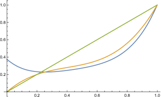
Figure 3: The graphs of $f_{n}$ for $n=4$ (blue), $n=3$ (orange)

Lemma 3.3

For all $n\geq 2$, the function $f_{n}$ admits in $(0,1)$ a unique fixed point $\alpha_{n}$, and $\alpha_{n}<\nicefrac{{1}}{{2}}$.

Proof. To prove the unicity, we have to distinguish two cases according to the parity of $n$.

• Odd case (see the orange graph of Figure 3):
  Using Lemma 3.1, Remark 3.2 and (3.2) , we have:

  $$f_{n}(0) =\frac{1}{\pi}\int_{0}^{\pi}\cos^{n}x\mathrm{d}x=0\ \ \text{and}\ \ f_{n}(1)=\frac{1}{\pi}\int_{0}^{\pi}\mathrm{d}x=1,$$ (3.5)

  $$f_{n}^{\prime}(0) =\frac{n}{\pi}\left(\int_{0}^{\pi}\cos^{n-1}x\mathrm{d}x-\int_{0}^{\pi}\cos^{n}x\mathrm{d}x\right)=\frac{n}{2^{n-1}}\binom{n-1}{\frac{n-1}{2}}>1,$$ (3.6)

  $$f_{n}^{\prime}(1) =\frac{n}{\pi}\int_{0}^{\pi}(1-\cos x)\mathrm{d}x=n>1,$$ (3.7)

  implying that $f_{n}$ has at least one fixed point in $(0,1)$. The inequality in (3.6) follows from (see (6.6))

  $$\forall n\geq 1,\ \ \ {\frac{2}{\sqrt{2\pi(2n+1)}}}<\xi_{2n}:=\frac{1}{2^{2n}}\binom{2n}{n}$$ (3.8)

  Note also that the formulas (3.5) are direct with the spreading rules.
  Moreover, Remark 3.2 with $k=3$ gives (note that $n\geq 3$ since $n$ is odd):

  $$\forall t\in[0,1],\ \ f_{n}^{(3)}(t)=\frac{1}{\pi}\frac{n!}{(n-3)!}\int_{0}^{\pi}(1-\cos x)^{3}(t(1-\cos x)+\cos x)^{n-3}\mathrm{d}x>0,$$

  implying that $f_{n}$ has at most three fixed points in $[0,1]$. As a result, $f_{n}$ has a unique fixed point $\alpha_{n}$ in $(0,1)$.

• Even case (see the blue graph of Figure 3):
  Since $f_{n}(0)=\frac{1}{2^{n}}\binom{n}{\frac{n}{2}}>0$, $f_{n}(1)=1$ and $f_{n}^{\prime}(1)=n>1$, we deduce that $f_{n}$ has at least one fixed point in $(0,1)$. Using again Remark 3.2, $f_{n}$ is strictly convex in $[0,1]$ and has thus at most two fixed points in this interval. As a result, $f_{n}$ has a unique fixed point $\alpha_{n}$ in $(0,1)$.

Thanks to the unicity of $\alpha_{n}$, we just have to show $f_{n}(\nicefrac{{1}}{{2}})<\nicefrac{{1}}{{2}}$ to obtain $\alpha_{n}<\nicefrac{{1}}{{2}}$.
According to the formula (6.3) of Lemma 6.2:

$$f_{n}\left(\frac{1}{2}\right)=\frac{1}{2^{n}}\sum_{k,0\leq 2k\leq n}2^{-2k}\binom{n}{2k}\binom{2k}{k}=\frac{1}{2^{2n}}\binom{2n}{n}=\xi_{2n}.$$ (3.9)

As $\xi_{2}=\nicefrac{{1}}{{2}}$ and $\left(\xi_{2n}\right)_{n\geq 0}$ is a strictly decreasing sequence according to Lemma 6.4, $\xi_{2n}<\nicefrac{{1}}{{2}}$ for all $n\geq 2$.   $\quad\square$

Remark 3.4

If we look at the GW case, we have to study the fixed points in $[0,1)$ of:

$$f:t\in[0,1]\mapsto\sum_{n\geq 2}q_{n}f_{n}(t).$$

With similar arguments as those of the previous proof, it is not difficult to prove the existence of a fixed point $\alpha\in(0,\nicefrac{{1}}{{2}})$, since

$$f(1)=1,\,f^{\prime}(1) =\mathbb{E}[N]>1,\ \ \text{and}\ \ f(\nicefrac{{1}}{{2}})<\nicefrac{{1}}{{2}}.$$

Indeed, if $f(0)=\sum_{n\geq 1}q_{2n}f_{2n}(0)>0$, we have our result and, otherwise, $q_{2n}=0$ for every $n\geq 1$, so $f^{\prime}(0)=\sum_{n\geq 1}q_{2n+1}f^{\prime}_{2n+1}(0)>1$ and we can easily conclude.

Moreover, if the support of $N$ is a subset of $2\mathbb{N}$ or of $2\mathbb{N}+1$, we have the unicity of $\alpha$ by the arguments used in the previous proof.

3.1 The odd case

3.1.1 Basin of attraction of the fixed point $\alpha_{n}$

Figure 4: The graphs of $f_{n}$ for $n=3$ (blue), $n=5$ (orange), $n=7$ (green) and $n=9$ (red), on $[0,1]$ and $[0,\nicefrac{{1}}{{5}}]$

Proposition 3.5

For all odd $n\geq 2$, $(0,1)$ is the basin of attraction of $\alpha_{n}$.

Proof. The unicity of the fixed point $\alpha_{n}$ and formulas (3.5)-(3.7) imply

$$f_{n}(x)>x,\forall x\in(0,\alpha_{n})\ \ \mbox{ and }\ \ f_{n}(x)<x,\forall x\in(\alpha_{n},1).$$ (3.10)

Now we define the recursive sequence $(u_{m})$ by $u_{0}=x_{0}$ and $u_{m+1}=f_{n}(u_{m})$ for $m\geq 0$. Since

$$\forall t\in[0,1]\,,\ \ f_{n}^{\prime}(t)=\frac{n}{\pi}\int_{0}^{\pi}(1-\cos x)(t(1-\cos x)+\cos x)^{n-1}\mathrm{d}x\ >\ 0,$$

the function $f_{n}$ is strictly increasing on $[0,1]$ and a simple reasoning shows that if $x_{0}\in(0,\alpha_{n})$, $(u_{m})$ is strictly increasing and bounded above by $\alpha_{n}$, and if $x_{0}\in(\alpha_{n},1)$, $(u_{m})$ is strictly decreasing and bounded below by $\alpha_{n}$. As a consequence, for all $x_{0}\in(0,1)$:

$$\lim_{m\rightarrow\infty}u_{m}=\alpha_{n}.$$

$\quad\square$

Remark 3.6

1. Note that the fixed point $\alpha_{n}$ of $f_{n}$ is a linearly attracting, i.e. $f^{\prime}_{n}(\alpha_{n})\in(-1,1)$. Indeed, it holds obviously $f^{\prime}_{n}(\alpha_{n})\in(0,1]$ by the preceding proof. Moreover, the equality $f^{\prime}_{n}(\alpha_{n})=1$ would imply that $\alpha_{n}$ is an inflection point of $f_{n}$ and then that $f^{(2)}_{n}(\alpha_{n})=0$, which would lead to $f_{n}(t)>t$ on $(\alpha_{n},1]$ since $f^{(2)}_{n}$ is strictly increasing on $[0,1]$, a contradiction.

2. The reasoning here can be applied for a GW with a reproduction law whose support is a subset of $2\mathbb{N}+1$. Indeed, the studied function $f=\sum_{n\geq 1}q_{2n+1}f_{2n+1}$ is then strictly increasing on $[0,1]$ and admits a unique fixed point on this interval.

3.1.2 Proof of Theorem 1.1 and Corollary 1.2

The case of a $n$-ary tree when $n\geq 3$ is odd

Note first that in this case, the statement of Theorem 1.1 is obvious when $\mathbf{p}_{1}=\mathbf{p}_{2}=\frac{1}{2}$, since $0$ is a fixed point of $f_{n}$ and thus $(0,\frac{1}{2},\frac{1}{2},0_{k-2})$ is a fixed point of $H$.

It thus remains to prove Theorem 1.1 in this case when $\mathbf{p}_{1}=\mathbf{p}_{2}\in(0,\frac{1}{2})$. To this end, let us fix $\mathbf{p}\in\mathscr{Q}_{k}$ (with $k\geq 2$) such that $\mathbf{p}_{1}=\mathbf{p}_{2}\in(0,\frac{1}{2})$ and $\mathbf{p}_{2}>\mathbf{p}_{3}\geq\dots\geq\mathbf{p}_{k}\geq 0$, and let us assume for a moment that there exists $\beta^{\prime}>0$ such that $\mathbf{p}_{0}(m)\geq\beta^{\prime}$ for every $m>0$. It then holds $0<\beta\leq\mathbf{p}_{1}(m)\leq\frac{1-\beta^{\prime}}{2}<\frac{1}{2}$ for every $m>0$. Thus, with the same arguments as those used in the proof of Proposition 2.8, but working now with the compact set $[\beta,\frac{1-\beta^{\prime}}{2}]\subset(0,\frac{1}{2})$ instead of $[\beta,\frac{1}{2}]$, one shows that

$$\mathbf{p}(m)\longrightarrow\left(\alpha_{n},\frac{1-\alpha_{n}}{2},\frac{1-\alpha_{n}}{2},0_{k-2}\right)\ \ \text{when $m\to\infty$}.$$

To conclude, let us then prove that when $\mathbf{p}_{1}=\mathbf{p}_{2}\in(0,\frac{1}{2})$, there exists $\beta^{\prime}>0$ such that $\mathbf{p}_{0}(m)\geq\beta^{\prime}$ for every $m>0$.

First, let us observe from the spreading rules that if $\mathbf{p}_{0}(\ell)>0$ for some $\ell\in\mathbb{N}$, then $\mathbf{p}_{0}(m)>0$ for every $m\geq\ell$. In particular, $\mathbf{p}_{0}(m)>0$ for every $m\in\mathbb{N}$ when $\mathbf{p}_{0}>0$ and, when $\mathbf{p}_{0}=0$, then $k\geq 3$ and $\mathbf{p}_{3}>0$, which implies $\mathbf{p}_{0}(1)>0$ (also from the spreading rules, since $n\geq 3$ is odd). Consequently: $\mathbf{p}_{0}(m)>0$ for every $m>0$.

Moreover, note from the spreading rules that for every $m>0$,

$$\mathbf{p}_{0}(m+1)=H_{0}(\mathbf{p}_{0}(m),\dots,\mathbf{p}_{k}(m)) \geq\sum_{k,0\leq 2k\leq n}\binom{n}{2k}\binom{2k}{k}\mathbf{p}_{1}^{2k}(m)\mathbf{p}_{0}^{n-2k}(m)\,.$$ (3.11)

Using now Remark 2.6 and $1-\mathbf{p}_{0}(m)\geq 2\beta$, note also that there exist $C=2\beta D>0$ and $a\in(0,1)$ such that for every $m>0$, $\sum_{\ell=3}^{k}\mathbf{p}_{\ell}(m)\leq Ca^{m}$ and thus

$$2\mathbf{p}_{1}(m)=1-\mathbf{p}_{0}(m)-\sum_{\ell=3}^{k}\mathbf{p}_{\ell}(m)\geq\big{(}1-\mathbf{p}_{0}(m)\big{)}\big{(}1-\frac{1}{2\beta}\sum_{\ell=3}^{k}\mathbf{p}_{\ell}(m)\big{)}\geq\big{(}1-\mathbf{p}_{0}(m)\big{)}\big{(}1-Da^{m}\big{)}\,.$$

Take $m_{0}\in\mathbb{N}^{*}$ and $b\in(a,1)$ such that $Da^{m}\leq b^{m}$ for every $m\geq m_{0}$. It then follows from (3.10) and (3.11) that:

$$\forall m\geq m_{0}\,,\ \ \ \mathbf{p}_{0}(m+1) \ \geq\ (1-b^{m})^{n}\sum_{k,0\leq 2k\leq n}\binom{n}{2k}\binom{2k}{k}\left(\frac{1-\mathbf{p}_{0}(m)}{2}\right)^{2k}\mathbf{p}_{0}^{n-2k}(m)$$

$$\ =\ (1-b^{m})^{n}f_{n}(\mathbf{p}_{0}(m))\ \geq\ (1-b^{m})^{n}\min\{\mathbf{p}_{0}(m),\alpha_{n}\}.$$

Reasoning by induction thus leads to:

$$\forall m\geq m_{0}\,,\ \ \ \mathbf{p}_{0}(m)\ \geq\ \min\{\mathbf{p}_{0}(m_{0}),\alpha_{n}\}\prod_{\ell=m_{0}}^{m-1}(1-b^{\ell})^{n}\ \geq\ \min\{\mathbf{p}_{0}(m_{0}),\alpha_{n}\}\,A^{n}\,,$$

where $A:=\prod_{\ell=m_{0}}^{+\infty}(1-b^{\ell})$ is positive since the convergence of the Neumann series $\sum_{\ell\geq m_{0}}b^{\ell}$ implies the one of $\sum_{\ell\geq m_{0}}\ln(1-b^{\ell})$ to the real negative number $B=\ln(A)$. It follows that for every $m>0$,

$$\mathbf{p}_{0}(m)\ \geq\ \beta^{\prime}:=\min\{A^{n}\alpha_{n},A^{n}\mathbf{p}_{0}(m_{0}),\mathbf{p}_{0}(m_{0}-1),\dots,\mathbf{p}_{0}(1)\}\ >\ 0\,,$$

which concludes the proof of Theorem 1.1 in the case of a $n$-ary tree when $n\geq 3$ is odd.

The general case of a GW tree supported in $2\mathbb{N}+1$

We now look at the function $f=\sum_{n\geq 1}q_{2n+1}f_{2n+1}$ and at the corresponding function $H$. As above, the statement of Corollary 1.2 is obvious when $\mathbf{p}_{1}=\mathbf{p}_{2}=\frac{1}{2}$, since $0$ is a fixed point of $f$ and thus $(0,\frac{1}{2},\frac{1}{2},0_{k-2})$ is a fixed point of $H$.

It thus just remains to prove it when $\mathbf{p}_{1}=\mathbf{p}_{2}\in(0,\frac{1}{2})$, so we fix $\mathbf{p}\in\mathscr{Q}_{k}$ (with $k\geq 2$) such that $\mathbf{p}_{1}=\mathbf{p}_{2}\in(0,\frac{1}{2})$ and $\mathbf{p}_{2}>\mathbf{p}_{3}\geq\dots\geq\mathbf{p}_{k}\geq 0$. Reasoning as we did above with a $n$-ary tree when $n\geq 3$ is odd, it is sufficient to show that there exists $\beta^{\prime}>0$ such that $\mathbf{p}_{0}(m)\geq\beta^{\prime}$ for every $m>0$.

To this end, note first that the relation $\sum\limits_{n\geq 1}q_{2n+1}f^{\prime}_{2n+1}(0)>1$ (see (3.6)) implies the existence of $n^{*}\in\mathbb{N}^{*}$ such that $\sum\limits_{1\leq n\leq n^{*}}q_{2n+1}f^{\prime}_{2n+1}(0)>1$. The function $\tilde{f}:=\sum\limits_{1\leq n\leq n^{*}}q_{2n+1}f_{2n+1}$ hence satisfies $\tilde{f}(0)=0$, $\tilde{f}^{\prime}(0)>1$, and $\tilde{f}\leq f$ on $[0,1]$, implying $\tilde{f}(1)\leq f(1)=1$. It thus admits at least one fixed point in $(0,1)$ and we define $\alpha^{*}$ as the smallest one. It follows that $\tilde{f}(x)>x$ on $(0,\alpha^{*})$ and, since $\tilde{f}$ is increasing on $[0,1]$, the function $\tilde{f}$ satisfies $\tilde{f}(x)\geq\min\{x,\alpha^{*}\}$ for every $x\in[0,1]$.

We can then conclude by following the same lines as above for a $n$-ary tree: again, the spreading rules imply that $\mathbf{p}_{0}(m)>0$ for every $m>0$ and that

$$\mathbf{p}_{0}(m+1)=H_{0}(\mathbf{p}_{0}(m),\dots,\mathbf{p}_{k}(m)) \geq\sum_{n\geq 1}q_{2n+1}\sum_{k,0\leq 2k\leq 2n+1}\binom{2n+1}{2k}\binom{2k}{k}\mathbf{p}_{1}^{2k}(m)\mathbf{p}_{0}^{2n+1-2k}(m)$$

$$\geq\sum_{n=1}^{n^{*}}q_{2n+1}\sum_{k,0\leq 2k\leq 2n+1}\binom{2n+1}{2k}\binom{2k}{k}\mathbf{p}_{1}^{2k}(m)\mathbf{p}_{0}^{2n+1-2k}(m)\,.$$

Reasoning as in the lines following (3.11) then implies the existence of $m_{0}\in\mathbb{N}^{*}$ and of $b\in(0,1)$ such that, for every $m\geq m_{0}$,

$$\mathbf{p}_{0}(m+1) \ \geq\ \sum_{n=1}^{n^{*}}q_{2n+1}(1-b^{m})^{2n+1}\sum_{k,0\leq 2k\leq 2n+1}\binom{2n+1}{2k}\binom{2k}{k}\left(\frac{1-\mathbf{p}_{0}(m)}{2}\right)^{2k}\mathbf{p}_{0}^{2n+1-2k}(m)$$

$$\ \geq\ (1-b^{m})^{2n^{*}+1}\tilde{f}(\mathbf{p}_{0}(m))\ \geq\ (1-b^{m})^{2n^{*}+1}\min\{\mathbf{p}_{0}(m),\alpha^{*}\}$$

and then

$$\mathbf{p}_{0}(m)\ \geq\ \min\{\mathbf{p}_{0}(m_{0}),\alpha^{*}\}\prod_{\ell=m_{0}}^{m-1}(1-b^{\ell})^{2n^{*}+1}\ \geq\ \min\{\mathbf{p}_{0}(m_{0}),\alpha^{*}\}\,\prod_{\ell=m_{0}}^{+\infty}(1-b^{\ell})^{2n^{*}+1}\ >\ 0\,.$$

This implies the existence of $\beta^{\prime}>0$ such that $\mathbf{p}_{0}(m)\geq\beta^{\prime}$ for every $m>0$ and then concludes the proof of Corollary 1.2.

3.2 The even case

3.2.1 The fixed point $\alpha_{n}$ is linearly attracting

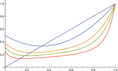
Figure 5: The graphs of $f_{n}$ for $n=2$ (blue), $n=4$ (orange), $n=6$ (green) and $n=10$ (red)

Proposition 3.7

For all even $n\geq 2$, $\alpha_{n}$ is linearly attracting.

The only difficulty to obtain this statement is to prove that $f^{\prime}_{n}(\alpha_{n})>-1$. Indeed, since $f_{n}(0)>0$ and $f_{n}^{\prime}(1)>1=f_{n}(1)$, the unicity of $\alpha_{n}$ leads to

$$f_{n}(x)>x,\forall x\in(0,\alpha_{n})\ \ \mbox{ and }\ \ f_{n}(x)<x,\forall x\in(\alpha_{n},1)\,,$$

and hence $f^{\prime}(\alpha_{n})\leq 1$. Since moreover $f$ is strictly convex on $[0,1]$, we have $f^{\prime}(\alpha_{n})<1$ since the equality $f^{\prime}(\alpha_{n})=1$ would imply $f_{n}(x)>x$ on $[0,1]$, a contradiction.

A direct proof of Proposition 3.7 using integral estimates relying on the relation (3.1) is proposed in the following subsection. Nevertheless, we would like to point out that we have come up with a totally independent proof using Budan’s theorem:

Theorem 3.8

(of Budan-Fourier)[3] Let $P(x)=0$ be a polynomial equation with real coefficients of degree $n$ and let $a<b$ be any two real numbers. Then, there exists $k\in\mathbb{N}$ such that the number of roots (counted with multiplicity) of this equation in the interval $(a,b]$ is equal to

$$V_{a}(P)-V_{b}(P)-2k\,,$$

where, for $c\in\mathbb{R}$, $V_{c}(P)$ is the number of sign variations in the sequence $P(c),P^{\prime}(c),\dots,P^{(n)}(c)$.

This proof has its own interest since it can be applied to prove the attractivity of a fixed point in the more general setting of GW, see Remark 3.10. It relies on the

Lemma 3.9

For all even $n\geq 2$, the function

$$\gamma:t\in[0,1]\longmapsto tf_{n}(t)=\sum_{k,0\leq 2k\leq n}\binom{n}{2k}\binom{2k}{k}\left(\frac{1-t}{2}\right)^{2k}t^{n+1-2k}\in\mathbb{R},$$

is strictly increasing on $(0,\nicefrac{{1}}{{2}})$.

Proof. Writing:

$$\left(\left({1-t}\right)^{2k}t^{n+1-2k}\right)^{\prime} =t^{n}\left(\frac{1-t}{t}\right)^{2k-1}\left(\frac{1}{t}(n+1-2k)-(n+1)\right),$$

the inequality $\gamma^{\prime}(t)>0$ for $t\in(0,\nicefrac{{1}}{{2}})$ is equivalent to:

$$\forall\,t\,\in\,\left(0,\nicefrac{{1}}{{2}}\right)\,,\ \ \ \sum_{k,0\leq 2k\leq n}2^{-2k}\binom{n}{2k}\binom{2k}{k}\left(\frac{1-t}{t}\right)^{2k-1}\left(\frac{1}{t}(n+1-2k)-(n+1)\right)>0.$$

Using the substitution $s=\frac{1-t}{t}\Leftrightarrow t=\frac{1}{1+s}$, it is equivalent to prove on $(1,+\infty)$:

$$g(s): =\sum_{k,0\leq 2k\leq n}2^{-2k}\binom{n}{2k}\binom{2k}{k}s^{2k-1}\left((1+s)(n+1-2k)-(n+1)\right)$$

$$=\sum_{k,0\leq 2k\leq n}2^{-2k}\binom{n}{2k}\binom{2k}{k}s^{2k-1}\left(s(n+1-2k)-2k\right)>0.$$

In order to use Theorem 3.8, we need the $\ell$-th derivatives of the function $g$ for $0\leq\ell\leq n$ and their values at the limits of the interval $(1,+\infty)$. As:

$$\frac{\mathrm{d}^{\ell}}{\mathrm{d}s^{\ell}}(s^{2k}) =\frac{(2k)!}{(2k-\ell)!}s^{2k-\ell},$$

$$\frac{\mathrm{d}^{\ell}}{\mathrm{d}s^{\ell}}(2ks^{2k-1}) =\frac{(2k)!}{(2k-\ell)!}(2k-\ell)s^{2k-\ell-1},$$

$$\binom{n}{2k} =\frac{n!}{(n-\ell)!}\binom{n-\ell}{2k-\ell}\frac{(2k-\ell)!}{(2k)!},$$

we obtain:

$$g^{(\ell)}(s)=\frac{n!}{(n-\ell)!}\sum_{k,\ell\leq 2k\leq n}2^{-2k}\binom{2k}{k}\binom{n-\ell}{2k-\ell}s^{2k-\ell-1}\left(s(n+1-2k)-(2k-\ell)\right).$$ (3.12)

Since $n$ is even and $2k\leq n$ for every $k$ considered in the sum in (3.12),

$$g^{(\ell)}(s)\underset{s\rightarrow\infty}{\sim}s^{n-\ell}2^{-n}\binom{n}{\frac{n}{2}}\frac{n!}{(n-\ell)!}>0,\forall\ell\in\llbracket 0,n\rrbracket.$$

Moreover, according again to (3.12), for every $\ell\in\llbracket 0,n\rrbracket$:

$$g^{(\ell)}(1)=\frac{n!}{(n-\ell)!}\sum_{k,\ell\leq 2k\leq n}2^{-2k}\binom{2k}{k}\binom{n-\ell}{2k-\ell}\left(n+1+\ell-4k\right).$$

The sign of $g^{(\ell)}(1)$, and thus of

$$\sum_{k,\ell\leq 2k\leq n}2^{-2k}\binom{2k}{k}\binom{n-\ell}{2k-\ell}\left(n+1+\ell-4k\right):=\sum_{k,\ell\leq 2k\leq n}\mu_{k}\alpha_{k}\,,$$

where $\alpha_{k}:=n+1+\ell-4k$, is difficult to obtain directly. As $(\alpha_{k})_{k\geq 0}$ is a decreasing sequence, the main idea is to use Lemma 6.1 to bound below this sum with a quantity that we are able to compute. Defining

$$\nu_{k}:=\binom{n-\ell}{2k-\ell},\ \ \text{it holds}\ \ \frac{\mu_{k}}{\nu_{k}}={2}^{-2k}\binom{2k}{k}=\xi_{2k}\,,$$

and, as $\left(\xi_{2k}\right)_{k\geq 0}$ is a decreasing sequence (see Lemma 6.4), we can apply Lemma 6.1 which gives:

$$\frac{\sum_{k,\ell\leq 2k\leq n}\mu_{k}\alpha_{k}}{\sum_{k,\ell\leq 2k\leq n}\mu_{k}}\geq\frac{\sum_{k,\ell\leq 2k\leq n}\nu_{k}\alpha_{k}}{\sum_{k,\ell\leq 2k\leq n}\nu_{k}}=\frac{\sum_{k,\ell\leq 2k\leq n}\binom{n-\ell}{2k-\ell}(n+1+\ell-4k)}{\sum_{k,\ell\leq 2k\leq n}\binom{n-\ell}{2k-\ell}}.$$

Moreover, according to (6.2) and to (6.4):

$$\sum_{k,\ell\leq 2k\leq n}\nu_{k}\alpha_{k} =(n-\ell+1)\sum_{k,\ell\leq 2k\leq n}\binom{n-\ell}{2k-\ell}-2\sum_{k,\ell\leq 2k\leq n}\binom{n-\ell}{2k-\ell}(2k-\ell)$$

$$=\begin{cases}(n-\ell+1)2^{n-\ell-1}-2(n-\ell)2^{n-\ell-2}\ &\text{if}\ \ell\in\{0,\dots,n-2\},\\ (n-\ell+1)2^{n-\ell-1}-2\ &\text{if}\ \ell=n-1,\\ 1\ &\text{if}\ \ell=n,\end{cases}$$

$$=\begin{cases}2^{n-\ell-1}\ &\text{if}\ \ell\in\{0,\dots,n-2\},\\ 0\ &\text{if}\ \ell=n-1,\\ 1\ &\text{if}\ \ell=n.\end{cases}$$

It follows that $g^{(\ell)}(1)\geq 0$ for every $\ell\in\llbracket 0,n\rrbracket$, so we have proved that $g^{(\ell)}(1)$ and $g^{(\ell)}(+\infty)$ have always the same sign. According to Theorem 3.8, the number of roots of $g$ in $(1,+\infty)$ is thus zero and hence $g>0$ on $(1,+\infty)$ since $\lim\limits_{t\to+\infty}g(t)=+\infty$.   $\quad\square$

Proof of Proposition 3.7
Using $f_{n}(\alpha_{n})<1$ and Lemma 3.9, the proof of Proposition 3.7 is straightforward:

$$\forall\,t\,\in\,(0,\nicefrac{{1}}{{2}})\,,\ \ \ \gamma^{\prime}(t)=f_{n}(t)+tf_{n}^{\prime}(t)>0\Leftrightarrow f_{n}^{\prime}(t)>-\frac{f_{n}(t)}{t},$$

and taking $t=\alpha_{n}$ leads to $f_{n}^{\prime}(\alpha_{n})>-1$.

Remark 3.10

The statement of Lemma 3.9 remains actually true when $n\geq 2$ is odd. It follows that in the GW case, the function

$$t\mapsto tf(t)=\sum_{n\geq 2}q_{n}tf_{n}(t)$$

is strictly increasing on $(0,\nicefrac{{1}}{{2}})$. In particular, we have $f^{\prime}(\alpha)>-1$ for every fixed point $\alpha\in(0,\frac{1}{2})$.
Recall moreover (Remark 3.4) that $f$ admits at least one fixed point in $(0,\frac{1}{2})$ and that, either $f(0)=0$ and $f^{\prime}(0)>1$, or $f(0)>0$. Hence, denoting by $\alpha$ the smallest fixed point in $(0,\frac{1}{2})$, we have necessarily $-1<f^{\prime}(\alpha)\leq 1$, which almost implies the linear attractivity of $\alpha$.
Furthermore, when the support of $q$ is included in $2\mathbb{N}$, the convexity of $f$ implies the attractivity of its unique fixed point.

3.2.2 Basin of attraction of the fixed point $\alpha_{n}$

The attractivity of $\alpha_{n}$ is not enough to obtain the even case in Theorem 1.1. In order to apply Proposition 2.8, we have to prove that the basin of attraction of $\alpha_{n}$ is $[0,1)$.

The proof is carried out in two steps. First, we prove the existence of $n_{0}\in\mathbb{N}$ such that $f_{n}^{\prime}(\alpha_{n})>0$ for every even $n>n_{0}$, which implies that the basin of attraction of $\alpha_{n}$ is $[0,1)$ when $n>n_{0}$. Secondly, we prove numerically that the basin of attraction of $\alpha_{n}$ is also $[0,1)$ for every even $2\leq n\leq n_{0}$. Moreover, we estimate the constants appearing in the computations with precision in order to minimize $n_{0}$ and then the number of values of $n$ for which we have to check the result numerically.

Lemma 3.11

For all even $n\in\mathbb{N}^{*}$ and all $t\in[0,1]$,

$$f_{n}(t)\geq\frac{1}{\sqrt{2\pi(n+1)}}\,.$$ (3.13)

Proof. Let us simply note that for every even $n\in\mathbb{N}^{*}$ and every $t\in[0,1]$,

$$f_{n}(t) = \frac{1}{\pi}\int_{0}^{\frac{\pi}{2}}\left((1-t)\cos{x}+t\right)^{n}{\rm d}x+\frac{1}{\pi}\int_{\frac{\pi}{2}}^{\pi}\left((1-t)\cos{x}+t\right)^{n}{\rm d}x$$

$$\geq \frac{1}{\pi}\int_{0}^{\frac{\pi}{2}}\cos^{n}{x}{\rm d}x\geq\frac{1}{\sqrt{2\pi(n+1)}},$$

where the last inequality follows from standard estimates on Wallis integrals, see (6.5).   $\quad\square$

Remark 3.12

Lemma 3.11 implies in particular $\alpha_{n}\geq\frac{1}{\sqrt{2\pi(n+1)}}$ for every even $n\in\mathbb{N}^{*}$.

Let us now recall two classical results, obtained by integration by parts, which will be useful in the sequel: if $X$ follows the standard normal distribution, then

$$\forall x>0\,,\ \ \mathbb{P}(X\geq x) =\frac{1}{\sqrt{2\pi}}\int_{x}^{\infty}e^{-\frac{u^{2}}{2}}\mathrm{d}u\leq\frac{e^{-\frac{x^{2}}{2}}}{x\sqrt{2\pi}},$$ (3.14)

$$\text{and}\qquad\forall n\in\mathbb{N}\,,\ \ \mathbb{E}\left[X^{2n}\right] =\frac{(2n)!}{2^{n}n!}.$$ (3.15)

On one hand, using (3.14):

$$\frac{1}{\pi}\int_{0}^{1}e^{-n\frac{x^{2}}{2}}{\rm d}x =\sqrt{\frac{2}{n\pi}}\left(\frac{1}{\sqrt{2\pi}}\int_{0}^{\sqrt{n}}e^{-\frac{u^{2}}{2}}\mathrm{d}u\right)=\sqrt{\frac{2}{n\pi}}\left(\frac{1}{2}-\mathbb{P}(X\geq\sqrt{n})\right)$$

$$\geq\sqrt{\frac{2}{n\pi}}\left(\frac{1}{2}-\frac{e^{-\frac{n}{2}}}{\sqrt{2\pi n}}\right)=\frac{1}{\sqrt{2\pi n}}-\frac{e^{-\frac{n}{2}}}{\pi n}.$$

Lemma 3.13

There exists $n_{0}\in\mathbb{N}$ such that for all even $n>n_{0}$, we have $f_{n}^{\prime}\left(\frac{1}{\sqrt{2\pi(n+1)}}\right)>0$.

Proof. Recall that:

$$f_{n}^{\prime}(x)=\frac{n}{\pi}\int_{0}^{\pi}(1-\cos{t})\left((1-x)\cos{t}+x\right)^{n-1}{\rm d}t.$$

Let $\zeta_{n}=\frac{1}{\sqrt{2\pi(n+1)}}$. We have

$$\frac{\pi}{n}f_{n}^{\prime}(\zeta_{n})= \displaystyle\int_{0}^{1}(1-\cos{t})\left((1-\zeta_{n})\cos{t}+\zeta_{n}\right)^{n-1}{\rm d}t +\int_{1}^{\pi}(1-\cos{t})\left((1-\zeta_{n})\cos{t}+\zeta_{n}\right)^{n-1}{\rm d}t$$

$$= A +\hskip 85.35826ptB.$$

Using successively that $\cos u\leq 1-\nicefrac{{u^{2}}}{{2}}+\nicefrac{{u^{4}}}{{4!}}$, $\cos u\geq 1-\nicefrac{{u^{2}}}{{2}}$, and $\ln(1-\nicefrac{{u^{2}}}{{2}})+\nicefrac{{u^{2}}}{{2}}\geq-\nicefrac{{u^{4}}}{{4}}$ on $[0,1]$, and $e^{u}-1\geq u$ on $\mathbb{R}$, we obtain

$$A = \int_{0}^{1}(1-\cos{t})\left((1-\zeta_{n})\cos{t}+\zeta_{n}\right)^{n-1}{\rm d}t\geq\int_{0}^{1}\left(\frac{t^{2}}{2}-\frac{t^{4}}{4!}\right)e^{(n-1)\ln(\cos{t})}{\rm d}t$$

$$\geq \int_{0}^{1}\left(\frac{t^{2}}{2}-\frac{t^{4}}{4!}\right)e^{-(n-1)\frac{t^{2}}{2}}{\rm d}t-(n-1)\int_{0}^{1}\left(\frac{t^{2}}{2}-\frac{t^{4}}{4!}\right)\frac{t^{4}}{4}e^{-(n-1)\frac{t^{2}}{2}}{\rm d}t$$

$$\geq \int_{0}^{1}\left(\frac{t^{2}}{2}-\frac{t^{4}}{4!}\right)e^{-(n-1)\frac{t^{2}}{2}}{\rm d}t-(n-1)\int_{0}^{1}\frac{t^{6}}{8}e^{-(n-1)\frac{t^{2}}{2}}{\rm d}t$$

$$\geq \int_{0}^{1}\frac{t^{2}}{2}e^{-(n-1)\frac{t^{2}}{2}}{\rm d}t-\int_{0}^{1}\frac{t^{4}}{4!}e^{-(n-1)\frac{t^{2}}{2}}{\rm d}t-(n-1)\int_{0}^{1}\frac{t^{6}}{8}e^{-(n-1)\frac{t^{2}}{2}}{\rm d}t=:D-(E+F).$$

It is an easy task to see that with the substitution $u=t\sqrt{n-1}$ and (3.15):

$$\frac{E+F}{\sqrt{2\pi}}\leq(n-1)^{-\nicefrac{{5}}{{2}}}\left(\frac{\mathbb{E}[X^{4}]}{2\times 4!}+\frac{\mathbb{E}[X^{6}]}{16}\right)=(n-1)^{-\nicefrac{{5}}{{2}}}.$$ (3.16)

In order to bound below $D$, we use integration by parts, (3.15) and (3.14):

$$\frac{D}{\sqrt{2\pi}} =(n-1)^{-\nicefrac{{3}}{{2}}}\frac{1}{2\sqrt{2\pi}}\int_{0}^{\sqrt{n-1}}u^{2}e^{-\frac{u^{2}}{2}}{\rm d}u=(n-1)^{-\nicefrac{{3}}{{2}}}\left(\frac{\mathbb{E}[X^{2}]}{4}-\frac{1}{2\sqrt{2\pi}}\int_{\sqrt{n-1}}^{\infty}u^{2}e^{-\frac{u^{2}}{2}}{\rm d}u\right)$$

$$=(n-1)^{-\nicefrac{{3}}{{2}}}\left(\frac{1}{4}-\frac{1}{2\sqrt{2\pi}}\left(\sqrt{n-1}e^{-\frac{n-1}{2}}+\int_{\sqrt{n-1}}^{\infty}e^{-\frac{u^{2}}{2}}{\rm d}u\right)\right)$$

$$\geq(n-1)^{-\nicefrac{{3}}{{2}}}\left(\frac{1}{4}-\frac{1}{2\sqrt{2\pi}}\left(\sqrt{n-1}e^{-\frac{n-1}{2}}+\frac{e^{-\frac{n-1}{2}}}{\sqrt{n-1}}\right)\right)$$

$$=(n-1)^{-\nicefrac{{3}}{{2}}}\left(\frac{1}{4}-\frac{n}{2\sqrt{2\pi(n-1)}}e^{-\frac{n-1}{2}}\right).$$ (3.17)

Let us now turn to $B$ and denote by $\mathscr{M}:=\left\{t\in[1,\pi],(1-\zeta_{n})\cos{t}+\zeta_{n}<0\right\}$. Since $n-1$ is odd, we have:

$$B =\int_{1}^{\pi}(1-\cos{t})\left((1-\zeta_{n})\cos{t}+\zeta_{n}\right)^{n-1}{\rm d}t\geq\int_{\mathscr{M}}(1-\cos{t})\left((1-\zeta_{n})\cos{t}+\zeta_{n}\right)^{n-1}{\rm d}t$$

$$\geq\int_{\frac{\pi}{2}}^{\pi}(1-\cos{t})(1-\zeta_{n})^{n-1}\left(\cos{t}\right)^{n-1}{\rm d}t=-(1-\zeta_{n})^{n-1}\left(W_{n}+W_{n-1}\right),$$

where $W_{n}$ is the Wallis integral. As $(1-\zeta_{n})^{n-1}\leq e^{-{\frac{n-1}{\sqrt{2\pi(n+1)}}}}$ and $(W_{n})$ is a decreasing sequence such that for all $n\geq 1$, $W_{n}\leq\sqrt{\frac{\pi}{2n}}$:

$$B\geq-2W_{n-1}e^{-{\frac{n-1}{\sqrt{2\pi(n+1)}}}}\geq-\sqrt{\frac{{2\pi}}{n-1}}e^{-{\frac{n-1}{\sqrt{2\pi(n+1)}}}}.$$ (3.18)

Combining (3.16), (3.2.2), and (3.18) yields

$$\frac{\pi}{n}f_{n}^{\prime}(\zeta_{n}) \geq\sqrt{2\pi}(n-1)^{-\nicefrac{{3}}{{2}}}\left(\frac{1}{4}-\frac{n}{2\sqrt{2\pi(n-1)}}e^{-\frac{n-1}{2}}-\frac{1}{(n-1)}-(n-1)e^{-{\frac{n-1}{\sqrt{2\pi(n+1)}}}}\right)$$

$$=\sqrt{2\pi}(n-1)^{-\nicefrac{{3}}{{2}}}\left(\frac{1}{4}-w_{n}\right).$$

The statement of Proposition 3.13 follows, since $\lim_{n\rightarrow\infty}w_{n}=0$.   $\quad\square$

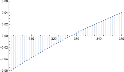
Figure 6: $\frac{1}{4}-w_{n}$.

We introduce the following notation for every even $n\geq 2$: we denote by

$$\hat{x}_{n}:=\operatorname*{arg\,min}_{x\in[0,1]}f_{n}(x)$$ (3.19)

the global minimum of the function $f_{n}$ on $[0,1]$. Note that the strict convexity of $f_{n}$ (as $n$ is even) together with $f_{n}^{\prime}(0)<0<f^{\prime}_{n}(1)$ ensures that $\hat{x}_{n}$ is unique and belong to $(0,1)$, with $f_{n}^{\prime}(\hat{x}_{n})=0$.

Lemma 3.14

For every even $n\in\mathbb{N}^{*}$ such that $f^{\prime}_{n}(\alpha_{n})>0$, the basin of attraction of $\alpha_{n}$ is $[0,1)$. This is in particular the case for every even $n$ sufficiently large.

Proof. The second part of Lemma 3.14 is an immediate consequence of its first part and of the convexity of $f_{n}$ together with Lemmas 3.11 and 3.13, which imply $f^{\prime}_{n}(\alpha_{n})>0$ for every even $n$ large enough.

Let us then prove the first part of this lemma. Thanks to the convexity of $f_{n}$, we have $0<\hat{x}_{n}<\alpha_{n}$ and then $f_{n}(\hat{x}_{n})>\hat{x}_{n}$. We drop the subscript _n in the rest of the proof below to lighten the notation and we define the recursive sequence $(u_{m})_{m\geq 0}$ by $u_{0}=x_{0}\in[0,1)$ and $u_{m+1}=f_{n}(u_{m})$ for $m\geq 0$.
On $[\alpha,1)$: $f$ is increasing, $f([\alpha,1))=[\alpha,1)$, and $f(x)\leq x$.
Thus, if $x_{0}\in[\alpha,1)$, the sequence $(u_{m})$ is decreasing and bounded below by $\alpha$, implying that $(u_{m})$ tends to $\alpha$, the fixed point of $f$ in $[\alpha,1)$.
On $[f(\hat{x}),\alpha)\subset(\hat{x},\alpha)$: $f$ is increasing, $f([f(\hat{x}),\alpha))\subset[f(\hat{x}),\alpha)$, and $f(x)>x$.
Thus, if $x_{0}\in[f(\hat{x}),\alpha)$, the sequence $(u_{m})$ is increasing and bounded above by $\alpha$, implying that $(u_{m})$ tends to $\alpha$, the fixed point of $f$ in $[f(\hat{x}),\alpha]$.
On $[\hat{x},f(\hat{x}))$: $f$ is increasing and $f([\hat{x},f(\hat{x}))\subset[f(\hat{x}),1)$.
We can thus conclude with the two previous cases when $x_{0}\in[\hat{x},f(\hat{x}))$.
On $[0,\hat{x})$: $f$ is decreasing and $f([0,\hat{x}))=(f(\hat{x}),f(0)]\subset[f(\hat{x}),1)$.
We can thus again conclude with the two first cases when $x_{0}\in[0,\hat{x})$.   $\quad\square$

Remark 3.15

In the general GW setting, if the function $f=\sum_{n}q_{n}f_{n}$ is strictly convex, using previous arguments we get existence and unicity of the fixed point $\alpha$ in $[0,1)$. If in addition $f^{\prime}(\alpha)\geq 0$, the basin of attraction of $\alpha$ is $[0,1)$ with a similar reasoning as in the proof of Lemma 3.14.

3.2.3 Proof of Theorem 1.1 in the even case

Proof in the even case when $n>26$.

Let us observe that the sequence $(w_{n})$ converging to $0$ defined at the end of the proof of Lemma 3.13 is decreasing for $n$ large enough. More precisely,

$$w_{n} =\frac{\sqrt{n-1}}{2\sqrt{2\pi}}e^{-\frac{n-1}{2}}+\frac{1}{2\sqrt{2\pi}}e^{-\frac{n-1}{2}}+\frac{1}{(n-1)}+(n-1)e^{-{\frac{n-1}{\sqrt{2\pi(n+1)}}}}$$

$$=w_{n}^{\prime}+(n-1)e^{-{\frac{n-1}{\sqrt{2\pi(n+1)}}}}$$

where $w_{n}^{\prime}$ is decreasing for all $n>1$.
On the other hand, the derivative of the function $x\mapsto(x-1)e^{-{\frac{x-1}{\sqrt{2\pi(x+1)}}}}$ is decreasing for $x>\frac{9}{2}\pi$ and negative at $x=26$ and hence $(w_{n})$ is decreasing for $n\geq 26$.

In particular, taking any $n_{0}\geq 26$ such that $\frac{1}{4}-w_{n_{0}}>0$, one has $f_{n}^{\prime}(\zeta_{n})>0$ and then $f_{n}^{\prime}(\alpha_{n})>0$ for every even $n\geq n_{0}$. It is also easy to check numerically that $\frac{1}{4}-w_{350}>0$ (see the right graph in Figure 6), and thus $f_{n}^{\prime}(\alpha_{n})>0$ for every even $n\geq 350$.

Moreover, computer assisted estimates show that $f_{n}^{\prime}(\alpha_{n})>0$ for every even $26<n<350$, see Figure 7 below.

Thus, $f_{n}^{\prime}(\alpha_{n})>0$ for every even $n>26$ and it follows from Lemma 3.14 that the basin of attraction of $\alpha_{n}$ is $[0,1)$ for every even $n>26$. The statement of Theorem 1.1 in this case is then a consequence of Proposition 2.8.

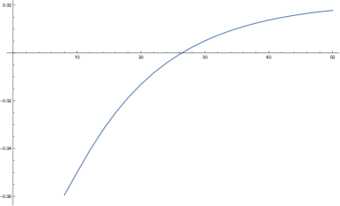
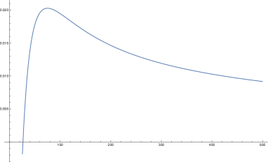
Figure 7: $f^{\prime}_{2n}(\alpha_{2n})$ for $n$ in $[2,250]$

Proof of Theorem 1.1 in the even case when $2\leq n\leq 26$.

Let us consider the case $n$ even and $f_{n}^{\prime}(\alpha_{n})<0$. The function $f_{n}$ being strictly convex on $[0,1]$, the inverse image $f_{n}^{-1}(\hat{x}_{n})$ of its minimum $\hat{x}_{n}$ is composed by at most two elements, $a_{n}<b_{n}\in[0,1]$ (see Figure 8).

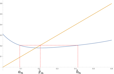
Figure 8: The graph of $f_{2}$

We have $\alpha_{n}<\hat{x}_{n}$ (since $f_{n}^{\prime}(\alpha_{n})<0$ and $f_{n}^{\prime}(\hat{x}_{n})=0$) and $f_{n}(\hat{x}_{n})<\hat{x}_{n}$ (since $\hat{x}_{n}>\alpha_{n}$, the unique fixed point in $(0,1)$). Note also that in the case of existence of $a_{n}$ and $b_{n}$, we have $0\leq a_{n}<\alpha_{n}<\hat{x}_{n}<b_{n}<1$. We have moreover in this case the following

Lemma 3.16

Assume the existence of $a_{n}$ and $b_{n}$ and that $k:=\max\big{(}\left|f_{n}^{\prime}(a_{n})|,|f_{n}^{\prime}(b_{n})\right|\big{)}<1$. Then, the basin of attraction of $\alpha_{n}$ is $[0,1)$.

Proof. For typographical simplicity we chose to not write the subscripts _n.
Note that $f([a,b])=[f(\hat{x}),\hat{x}]\subset[f(\hat{x}),b]$ since $f$ is decreasing on $[a,\hat{x}]$ and increasing on $[\hat{x},b]$. Moreover, using the convexity of $f$, first:

$$\hat{x}-f(\hat{x})=f(a)-f(\hat{x})\leq\left|f^{\prime}(a)\right|(\hat{x}-a)\leq\hat{x}-a\,,$$

implying that $f(\hat{x})\geq a$ and thus $f([a,b])\subset[a,b]$, and secondly: for every $x\in[a,b]$,

$$\left|f(x)-\alpha\right|=\left|f(x)-f(\alpha)\right|\leq\max_{a\leq y\leq b}\left|f^{\prime}(y)\right||x-\alpha|\leq k|x-\alpha|,$$

implying that the basin of attraction of $\alpha$ contains $[a,b]$.
Now, if $x\in(b,1)$, there exists $N\in\mathbb{N}^{*}$ such that $f^{N}(x)\leq b$ and for all $0\leq q<N,\,f^{q}(x)\in(b,1)$. Indeed, since $f(y)<y$ on $(b,1)$, if $N$ does not exist, the sequence $(f^{q}(x))_{q\geq 0}$ is decreasing and bounded below by $b$, so tends toward a fixed point of $f$ in $[b,1)$, which raises a contradiction.
As a result, the definition of $N$ and the monotonicity of $f$ on $(b,1)$ imply

$$a\leq\hat{x}=f(b)\leq f^{N}(x)\leq b$$

and we conclude that $(b,1)$ is included in the basin of attraction of $\alpha$ since $[a,b]$ is.
In particular, the basin of attraction of $\alpha$ contains $[a,1)$ and, as $f$ is decreasing on $[0,a)$, $f([0,a))=\left(\hat{x},f(0)\right]\subset[a,1)$, implying that $[0,a)$ and thus $[0,1)$ is included in the basin of attraction of $\alpha$.   $\quad\square$

The rest of the proof of Theorem 1.1 is obtained using computer assistance to find good approximations for the quantities $\hat{x}_{n}$, $f_{n}(\hat{x}_{n})$, $\alpha_{n}$, $f_{n}^{\prime}(\alpha_{n})$, $a_{n}$, $b_{n}$, $f_{n}^{\prime}(a_{n})$ and $f_{n}^{\prime}(b_{n})$: for every even $4\leq n\leq 26$, $a_{n}$ and $b_{n}$ exist and satisfy the assumptions of Lemma 3.16, see the following Table. Proposition 2.8 thus implies the statement of Theorem 1.1 in this case.

[separator=tab, tabular=|c|c|c|c|c|c|c|c|c|, table head=$n$ $\hat{x}_{n}$ $f_{n}(\hat{x}_{n})$ $\alpha_{n}$ $f_{n}^{\prime}(\alpha_{n})$ $a_{n}$ $b_{n}$ $f_{n}^{\prime}(a_{n})$ $f_{n}^{\prime}(b_{n})$, late after head=
, late after line=
] tableau9.csv n=, tmin=, fn(tmin)=, tfixe=, fn_prime(tfixe)=, t1=, t2=, fn_prime(t1)=, fn_prime(t2)=

Remark 3.17

1. Note that for $n\in\{28,30\}$, the cells corresponding to $a_{n}$ and $b_{n}$ are empty since no pre-image of $\hat{x}_{n}$ exists in these cases.

2. The strategy in this section can not be used for the case of a GW, whereas Lemma 3.9 implies the non-repulsivity of the fixed point which is a big step to achieve our goal if we succeed to prove the unicity of the fixed point.

3.3 Estimates on the fixed points $\alpha_{n}$

In this section we obtain bounds for the fixed points of $f_{n}$ depending on $n$. As previously, we denote for $n\in\mathbb{N}$, $\xi_{2n}=2^{-2n}\binom{2n}{n}$.

Proposition 3.18

We have:

$$\forall\,n\geq 536\,,\ \ \frac{1}{\sqrt{2\pi(n+\frac{1}{4})}}<\xi_{4n}\leq\alpha_{n}\quad\text{and}\quad\forall\,n\geq 3\,,\ \ \alpha_{n}\leq\xi_{n^{\#}}\leq\frac{\sqrt{2}}{\sqrt{\pi(n-1)}}\,,$$ (3.20)

where $n^{\#}:=2\left[\frac{n}{2}\right]$.

Proof. According to (see (6.6))

$$\forall n\geq 1\,,\ \ \ {\frac{2}{\sqrt{2\pi(2n+1)}}}<\xi_{2n}<{\frac{1}{\sqrt{\pi n}}},$$ (3.21)

we have just to prove lower bound $\xi_{4n}\leq\alpha_{n}$ for $n$ large enough and the upper bound $\alpha_{n}\leq\xi_{n^{\#}}$ for $n\geq 3$.

Using moreover the monotonicity of the sequence $\left(\xi_{2n}\right)$ and (6.4), we have for every $n\geq 2$:

$$\displaystyle f_{n}(\xi_{4n}) = \sum_{k,0\leq 2k\leq n}\binom{n}{2k}\xi_{2k}\left(1-\xi_{4n}\right)^{2k}\xi_{4n}^{n-2k}$$

$$\geq \sum_{k,0\leq 2k\leq n}\binom{n}{2k}\xi_{n^{\#}-2}\left(1-\xi_{4n}\right)^{2k}\xi_{4n}^{n-2k}+(\xi_{n^{\#}}-\xi_{n^{\#}-2})\binom{n}{n^{\#}}\left(1-\xi_{4n}\right)^{n^{\#}}\xi_{4n}^{n-n^{\#}}$$

$$\geq \xi_{n^{\#}-2}\frac{1+(-1)^{n}(1-2\xi_{4n})^{n}-2\frac{n}{n-1}\xi_{4n}\left(1-\xi_{4n}\right)^{n^{\#}}}{2}$$

$$= \xi_{{n}^{\#}}\frac{{n^{\#}}}{{n^{\#}}-1}\frac{1+(-1)^{n}(1-2\xi_{4n})^{n}-2\frac{n}{n-1}\xi_{4n}\left(1-\xi_{4n}\right)^{n^{\#}}}{2}$$

$$\geq \xi_{4n}\frac{{n^{\#}}}{{n^{\#}}-1}\frac{1+(-1)^{n}(1-2\xi_{4n})^{n}-2\frac{n}{n-1}\xi_{4n}\left(1-\xi_{4n}\right)^{n^{\#}}}{e^{\frac{3}{4n}}}\,,$$

where the last inequality arises from using twice (see (6.7))

$$\forall n\geq 1\,,\ \ \ \xi_{4n}<\frac{1}{\sqrt{2}}e^{\frac{1}{4n}}\xi_{2n}\,.$$ (3.22)

Using now the relations $e^{x}<1+\frac{4}{3}x$ for $x\leq\frac{1}{2}$, $(1-x)^{n}\leq e^{-nx}$ for $x\in[0,1]$, and (3.21), which implies ${\frac{1}{\sqrt{2\pi(n+\frac{1}{4})}}<\xi_{4n}<\frac{1}{\sqrt{2\pi n}}}$, we have:

$$\frac{1+(-1)^{n}(1-2\xi_{4n})^{n}-2{\frac{n}{n-1}}\xi_{4n}\left(1-\xi_{4n}\right)^{n^{\#}}}{e^{\frac{3}{4n}}} \geq\frac{1-(1-2\xi_{4n})^{n}-\frac{2}{\sqrt{2\pi n}}{\frac{n}{n-1}}\left(1-\xi_{4n}\right)^{n^{\#}}}{\frac{n+1}{n}}$$

$$\geq\frac{1-e^{-\frac{2n}{\sqrt{2\pi(n+\frac{1}{4})}}}-\frac{2}{\sqrt{2\pi n}}{\frac{n}{n-1}}e^{-\frac{n-1}{\sqrt{2\pi(n+\frac{1}{4})}}}}{\frac{n+1}{n}}$$

Finally we can check that

$$\frac{{n^{\#}}}{{n^{\#}}-1}\left(1-e^{-\frac{2n}{\sqrt{2\pi(n+\frac{1}{4})}}}-\frac{2}{\sqrt{2\pi n}}{\frac{n}{n-1}}e^{-\frac{n-1}{\sqrt{2\pi(n+\frac{1}{4})}}}\right)>{\frac{n+1}{n}}$$

for all $n$ sufficiently large, and computer assisted calculations show that ${n\geq 536}$ is sufficient.

Hence, we have $f_{n}(\xi_{4n})\geq\xi_{4n}$ and thus $\alpha_{n}\geq\xi_{4n}$ for every $n\geq 536$.

To obtain the upper bound of (3.20), let us write for $n\geq 2$:

$$f_{n}(\xi_{n^{\#}})=\sum_{k,0\leq 2k\leq n}\binom{n}{2k}\xi_{2k}\left(1-\xi_{{n^{\#}}}\right)^{2k}\xi_{{n^{\#}}}^{n-2k}=:\sum_{k,0\leq 2k\leq n}\nu_{k}\alpha_{k}\,,$$

where $\alpha_{k}:=\xi_{2k}$, and let $\mu_{k}:=\binom{n}{2k}$. The positive sequence $(\alpha_{k})_{k\geq 0}$ is decreasing according to Lemma 6.4, and writing

$$\frac{\nu_{k}}{\mu_{k}}=\left(\frac{1}{\xi_{{n^{\#}}}}-1\right)^{2k}\xi_{{n^{\#}}}^{n},$$

the positive sequence $(\nicefrac{{\nu_{k}}}{{\mu_{k}}})_{k\geq 0}$ is increasing. Then, Lemma 6.1 and the formulas (3.9), (6.4) give:

$$f_{n}(\xi_{n^{\#}})\leq\frac{\sum_{k,0\leq 2k\leq n}\mu_{k}\alpha_{k}}{\sum_{k,0\leq 2k\leq n}\mu_{k}}\sum_{k,0\leq 2k\leq n}\nu_{k}=\frac{2^{-n}\binom{2n}{n}}{2^{n-1}}\frac{1+(-1)^{n}(1-2\xi_{n^{\#}})^{n}}{2}\leq\xi_{2n}\left(1+(1-2\xi_{n^{\#}})^{n}\right).$$

Consequently, using in addition and $(1-x)^{n}\leq e^{-nx}$ for all $x\in[0,1]$ and the lower bound in (3.21):

$$\left(1-2\xi_{n^{\#}}\right)^{n}\leq e^{-2n\xi_{n^{\#}}}\leq{e^{-\frac{4n}{\sqrt{2\pi(n^{\#}+1)}}}}.$$

Then, with (3.22):

$$f_{n}(\xi_{n^{\#}})\leq\xi_{2n^{\#}}\left(1+{e^{-\frac{4n}{\sqrt{2\pi(n^{\#}+1)}}}}\right)\leq\xi_{n^{\#}}\frac{1}{\sqrt{2}}{e^{\frac{1}{2n^{\#}}}}\left(1+{e^{-\frac{4n}{\sqrt{2\pi(n^{\#}+1)}}}}\right)=:\xi_{n^{\#}}w_{n}.$$

Since $n^{\#}=n$ when $n$ is even and $n^{\#}=n-1$ when $n$ is odd, the sequences $(w_{2k})_{k\geq 1}$ and $(w_{2k+1})_{k\geq 1}$ are clearly decreasing and, as ${w_{3},w_{4}\leq 1}$, we have for every $n\geq 3$ : $f_{n}(\xi_{n^{\#}})\leq\xi_{n^{\#}}$ and thus $\alpha_{n}\leq\xi_{n^{\#}}$.   $\quad\square$

4 An Example of GW

All the simulations with a GW seem to show that there is a unique fixed point in $(0,1)$ and its basin of attraction is $(0,1)$. As we have already said, we have not been able to adapt the techniques of Section 3 to prove the uniqueness of the fixed point in a general framework. Nevertheless, we propose an example in which we are able to prove everything.
In this section, we assume that the reproduction law $N$ follows a shifted geometric distribution with parameter $p\in(0,1)$, in other words:

$$q_{n}=\mathbb{P}(N=n)=p(1-p)^{n-2},\forall n\geq 2.$$

This example is very satisfying as we can obtain explicit formulas. More precisely, we have the following:

Lemma 4.1

If $N=X+1$ where $X$ follows a geometric distribution with parameter $p\in(0,1)$, we have:

$$f(t)=\frac{p}{(1-p)^{2}}\left(-((1-p)t+1)+\frac{1}{(p(2-p+2t(p-1)))^{\frac{1}{2}}}\right).$$ (4.1)

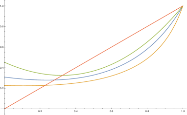
Figure 9: The graphs of $f$ for $p=\nicefrac{{1}}{{2}}$ (blue), $p=\nicefrac{{1}}{{4}}$ (orange), $p=\nicefrac{{9}}{{10}}$ (green)

Proof. We have:

$$f(t) =\sum_{n\geq 2}q_{n}f_{n}(t)=\sum_{n\geq 2}p(1-p)^{n-2}\frac{1}{\pi}\int_{0}^{\pi}((1-t)\cos x+t)^{n}\mathrm{d}x$$

$$=\frac{p}{\pi}\int_{0}^{\pi}((1-t)\cos x+t)^{2}\sum_{n\geq 2}(1-p)^{n-2}((1-t)\cos x+t)^{n-2}\mathrm{d}x$$

$$=\frac{p}{\pi}\int_{0}^{\pi}\frac{((1-t)\cos x+t)^{2}}{1-(1-p)((1-t)\cos x+t)}\mathrm{d}x=\frac{p}{\pi(1-p)^{2}}\int_{0}^{\pi}\frac{(1-p)^{2}((1-t)\cos x+t)^{2}-1+1}{1-(1-p)((1-t)\cos x+t)}\mathrm{d}x$$

$$=\frac{p}{\pi(1-p)^{2}}\int_{0}^{\pi}-(1-p)((1-t)\cos x+t)-1+\frac{1}{1-(1-p)((1-t)\cos x+t)}\mathrm{d}x$$

$$=\frac{-p((1-p)t+1)}{(1-p)^{2}}+\frac{p}{\pi(1-p)^{2}}\int_{0}^{\pi}\frac{\mathrm{d}x}{1-(1-p)((1-t)\cos x+t)}$$

With the substitution $u=\tan\frac{x}{2}$, we obtain:

$$\int_{0}^{\pi}\frac{\mathrm{d}x}{1-(1-p)((1-t)\cos x+t)} =2\int_{0}^{+\infty}\frac{\mathrm{d}u}{p+(2-p+2t(p-1))u^{2}}=\frac{2}{p}\int_{0}^{+\infty}\frac{\mathrm{d}u}{1+\frac{(2-p+2t(p-1))}{p}u^{2}}$$

$$=\frac{\pi}{(p(2-p+2t(p-1)))^{\frac{1}{2}}}.$$

Then

$$f(t)=\frac{p}{(1-p)^{2}}\left(-((1-p)t+1)+\frac{1}{(p(2-p+2t(p-1)))^{\frac{1}{2}}}\right).$$

$\quad\square$

In Figure 9, we can see that $f$ seems to have one fixed point on $(0,1)$. It is not difficult to find this point, resolving:

$$f(t)=t \Leftrightarrow-2(1-p)t^{3}+(2-5p)t^{2}+4pt-p=0\Leftrightarrow(t-1)(-2(1-p)t^{2}-3pt+p)=0$$

$$\Leftrightarrow t=1 \mbox{ or }t=\frac{-3p\pm(p(p+8))^{\frac{1}{2}}}{4(1-p)}.$$

And we can easily see that the only root that interests us is $\alpha=\frac{-3p+(p(p+8))^{\frac{1}{2}}}{4(1-p)}.$

Lemma 4.2

The basin of attraction of $\alpha$ is $[0,1)$.

Proof. The first and second derivative of $f$ are given by:

$$f^{\prime}(t)=\frac{p}{1-p}\left(-1+\frac{p}{(p(2-p+2t(p-1))^{\frac{3}{2}}}\right)\mbox{ and }f^{(2)}(t)=\frac{3p^{3}}{(p(2-p+2t(p-1))^{\frac{3}{2}}}.$$

As stated in Remark 3.15 since $f$ is strictly convex, it is sufficient to show that $f^{\prime}(\alpha)\geq 0$. One can see that:

$$f^{\prime}(\alpha)\geq 0 \Leftrightarrow\frac{p}{1-p}\left(-1+\frac{p}{(p(2-p-\frac{1}{2}(-3p+(p(p+8))^{\frac{1}{2}})))^{\frac{3}{2}}}\right)\geq 0$$

$$\Leftrightarrow 2^{\frac{3}{2}}p\geq(p(4+p-(p(p+8))^{\frac{1}{2}})))^{\frac{3}{2}}$$

$$\Leftrightarrow 2\geq p^{\frac{1}{3}}(4+p-(p(p+8))^{\frac{1}{2}}=:g(p).$$ (4.2)

As $g(1)=2$, if we prove that $g$ is an increasing function on $[0,1]$, we obtain formula (4). As:

$$g^{\prime}(p)=\frac{(4+p-(p(p+8))^{\frac{1}{2}})((p(p+8))^{\frac{1}{2}}-3p)}{3p^{\frac{2}{3}}(p(p+8))^{\frac{1}{2}}}$$

is obviously positive, our proof is complete.   $\quad\square$

To conclude, according to Proposition 2.8, for every $k\geq 2$ and $\mathbf{p}\in\mathscr{P}_{k}$ such that $\mathbf{p}_{1}=\mathbf{p}_{2}>\mathbf{p}_{3}\geq\dots\geq\mathbf{p}_{k}$, $\mathbf{p}(m)$ converges to $\left(\alpha,\frac{1-\alpha}{2},\frac{1-\alpha}{2},0_{k-2}\right)$ when $m\to\infty$.

Remark 4.3

Considering the $n$-ary tree as a GW tree with reproduction law $N=n$ a.s., we have $\mathbb{E}[N]=n$. In order to obtain the same mean in the geometric case, it suffices to take $p=\frac{1}{n-1}$. With this choice of $p$, $\alpha\sim\nicefrac{{1}}{{\sqrt{2n}}}$ when $n$ goes to infinity, which is consistent with the bounds found in Proposition 3.18.

5 Open questions and variant case

As a conclusion we make some remarks on the properties of the main objects studied in this work and discuss possible generalisations of our results.

1. One can notice in the figure 3, that the red curve of $f_{3}$, seems to cut the blue one $f_{4}$ at its minimum. In fact, that is true for all $n\geq 2$, that is:

   $$f_{2n}\left(\hat{x}_{2n}\right)=f_{2n-1}\left(\hat{x}_{2n}\right).$$ (5.1)

   Indeed, according to (3.4):

   $$f_{n}^{\prime}(t) =\frac{n}{\pi}\int_{0}^{\pi}(t(1-\cos x)+\cos x)^{n-1}\mathrm{d}x-\frac{n}{\pi}\int_{0}^{\pi}\cos x(t(1-\cos x)+\cos x)^{n-1}\mathrm{d}x$$

   $$=nf^{\prime}_{n-1}(t)-\frac{n}{\pi}\int_{0}^{\pi}\cos x(\cos x(1-t)+t)^{n-1}\mathrm{d}x$$

   $$=nf^{\prime}_{n-1}(t)-\frac{n}{\pi}\int_{0}^{\pi}\frac{\cos x(1-t)+t-t}{1-t}(\cos x(1-t)+t)^{n-1}\mathrm{d}x$$

   $$=n\left(1+\frac{t}{1-t}\right)f_{n-1}(t)-\frac{n}{1-t}f_{n}(t)\Leftrightarrow\frac{t-1}{n}f_{n}^{\prime}(t)=f_{n}(t)-f_{n-1}(t)$$ (5.2)

   and taking $t=\hat{x}_{2n}$:

   $$\frac{\hat{x}_{2n}-1}{n}f_{2n}^{\prime}(\hat{x}_{2n})=0=f_{2n}(\hat{x}_{2n})-f_{2n-1}(\hat{x}_{2n}).$$

   With an obvious induction reasoning, the formula (5.2) gives:

   $$f_{n}(t)-t=f_{n}(t)-f_{1}(t)=(t-1)\sum_{k={2}}^{n}\frac{1}{k}f_{k}^{\prime}(t).$$ (5.3)

   We think that these equalities have a probabilistic meaning, but did not manage to come up with an explanation.

2. The general GW case for two opinions seems for the moment out of reach, even though our simulations suggest that our results stay valid. Contrary to the article [5], the mean of the reproduction law $\mathbb{E}[N]$ does not seem to play a particular role: there seems to be always convergence.
   We have to study cases with more than two opinions: nevertheless, even in the case of a $n$-ary tree, using links with random walks in order to obtain formulas like (3.1) for a number $i>2$ of major opinions is not clear to us. Moreover, we have seen that even in the case with two opinions, parity plays an important role; already for $i=3$, the calculations become devilish and it seems to us that we need to find much finer methods than direct computations.
   For instance in Figure 10, we can see that the shape of the graph is linked to the remainder of the Euclidean division of $n$ by 3 and the equivalent formula for $f_{n}$ is:

   $$f_{n}(t) =\sum_{k=0}^{n}\binom{n}{3k}\binom{3k}{k}\binom{2k}{k}t^{n-3k}\left(\frac{1-t}{3}\right)^{3k}$$

   $$+3\sum_{k=0}^{n}\binom{n}{2k}\binom{2k}{k}\sum_{j=0}^{n-2k}\binom{n-2k}{j}t^{n-2k-j}\left(\frac{1-t}{3}\right)^{2k+j}.$$

   

   Figure 10: The graphs of $f_{n}$ for $n=7$ (blue), $n=9$ (orange), $n=11$ (green)

6 Appendix

In this appendix, we recall some classical definitions and results used throughout this paper.

The following result is crucial to prove the stability statement of Section 3.2.1.

Lemma 6.1

Consider two positive sequences $(\mu_{k})_{k\geq 0}$ and $(\nu_{k})_{k\geq 0}$ such that $\left(\nicefrac{{\nu_{k}}}{{\mu_{k}}}\right)_{k\geq 0}$ is increasing. Then, for every decreasing (resp. increasing) sequence $(\alpha_{k})_{k\geq 0}$ and for every $0\leq\ell\leq n$,

$$\frac{\sum_{k=\ell}^{n}\alpha_{k}\mu_{k}}{\sum_{k=\ell}^{n}\mu_{k}}\ \geq\ \frac{\sum_{k=\ell}^{n}\alpha_{k}\nu_{k}}{\sum_{k=\ell}^{n}\nu_{k}}\ \ \Big{(}\text{resp.}\ \leq\ \frac{\sum_{k=\ell}^{n}\alpha_{k}\nu_{k}}{\sum_{k=\ell}^{n}\nu_{k}}\ \Big{)}\,.$$ (6.1)

Proof. Assume that the sequence $\left(\nicefrac{{\nu_{k}}}{{\mu_{k}}}\right)_{k\geq 0}$ is increasing, which is equivalent to:

$$\forall\,0\leq i\leq j\,,\ \ \ {\mu_{i}\nu_{j}}\geq{\mu_{j}\nu_{i}}.$$

When the sequence $(\alpha_{k})_{k\geq 0}$ is decreasing, the formula (6.1) is equivalent to:

$$\sum_{i,j=\ell}^{n}\mu_{i}\alpha_{i}\nu_{j}\geq\sum_{i,j=\ell}^{n}\mu_{i}\alpha_{j}\nu_{j} \Leftrightarrow\sum_{\ell\leq i<j\leq n}\mu_{i}\alpha_{i}\nu_{j}+\sum_{\ell\leq j\leq i\leq n}\mu_{i}\alpha_{i}\nu_{j}\geq\sum_{\ell\leq i<j\leq n}\mu_{i}\alpha_{j}\nu_{j}+\sum_{\ell\leq j\leq i\leq n}\mu_{i}\alpha_{j}\nu_{j}$$

$$\Leftrightarrow\sum_{\ell\leq i<j\leq n}\mu_{i}\alpha_{i}\nu_{j}+\sum_{\ell\leq i\leq j\leq n}\mu_{j}\alpha_{j}\nu_{i}\geq\sum_{\ell\leq i<j\leq n}\mu_{i}\alpha_{j}\nu_{j}+\sum_{\ell\leq i\leq j\leq n}\mu_{j}\alpha_{i}\nu_{i}$$

$$\Leftrightarrow\sum_{\ell\leq i<j\leq n}\mu_{i}\alpha_{i}\nu_{j}+\sum_{\ell\leq i<j\leq n}\mu_{j}\alpha_{j}\nu_{i}\geq\sum_{\ell\leq i<j\leq n}\mu_{i}\alpha_{j}\nu_{j}+\sum_{\ell\leq i<j\leq n}\mu_{j}\alpha_{i}\nu_{i}$$

$$\Leftrightarrow\sum_{\ell\leq i<j\leq n}(\mu_{i}\nu_{j}-\mu_{j}\nu_{i})(\alpha_{i}-\alpha_{j})\geq 0\,,$$

which is true by hypothesis.   $\quad\square$

In the following lemma, we state classical results on binomial coefficients.

Lemma 6.2

For all $n\in\mathbb{N}$:

$$\sum_{k=0}^{n}(2k+1)\binom{n}{2k+1}=\sum_{k=0}^{n}2k\binom{n}{2k} =n2^{n-2}\ \ \text{ when $n\neq 1$}$$ (6.2)

$$\text{and}\qquad\sum_{j=0}^{n}\binom{n}{2j}\binom{2j}{j}2^{-2j} =2^{-n}\binom{2n}{n}\,.$$ (6.3)

Proof.

1. For all $x,y\in\mathbb{R}$ and $n\geq 0$, the relation

   $$h(x,y):=\sum_{k=0}^{n}\binom{n}{2k}x^{2k}y^{n-2k}=\frac{(x+y)^{n}+(y-x)^{n}}{2}$$ (6.4)

   implies that

   $$\frac{\partial h}{\partial x}(x,y)=\sum_{k=0}^{n}2k\binom{n}{2k}x^{2k-1}y^{n-2k}=\frac{n(x+y)^{n-1}-n(y-x)^{n-1}}{2}.$$

   Taking $x=y=1$ and $n\neq 1$, we obtain the right equality of (6.2).
   Moreover, with a very similar reasoning:

   $$g(x,y)=(x+y)^{n}=\sum_{k=0}^{n}\binom{n}{k}x^{k}y^{n-k}\mbox{ and }\frac{\partial g}{\partial x}(x,y)=n(x+y)^{n-1}=\sum_{k=0}^{n}\binom{n}{k}kx^{k-1}y^{n-k}$$

   and taking $x=y=1$, we obtain

   $$\sum_{k=0}^{n}\binom{n}{k}k=n2^{n-1}.$$

   We conclude by using

   $$\sum_{k=0}^{n}k\binom{n}{k}=\sum_{k=0}^{n}2k\binom{n}{2k}+\sum_{k=0}^{n}(2k+1)\binom{n}{2k+1}.$$

2. In [7], the author uses an expansion of $(x^{2}+2x)^{n}$ to prove (6.3) (see the formula (1.65) there). We will use here the following series expansion, for $\ell\in\mathbb{N}$ and $x\in[0,1)$ (which also permit to prove the generalization of (6.3) stated in Remark 6.3 below):

   $$\frac{x^{\ell}}{(1-x)^{\ell+1}}=\sum_{n\geq 0}\binom{n}{\ell}x^{n}\quad\text{and}\quad\frac{1}{\sqrt{1-x}}=\sum_{n\geq 0}\binom{2n}{n}2^{-2n}x^{n}.$$

   The first one can be obtained by induction and the second one is classical. Thus:

   $$\sum_{n\geq 0}\sum_{j\geq 0}\binom{n}{2j}\binom{2j}{j}2^{-2j}x^{n} = \sum_{j\geq 0}\binom{2j}{j}2^{-2j}\sum_{n\geq 0}\binom{n}{2j}x^{n}=\sum_{j\geq 0}\binom{2j}{j}2^{-2j}\frac{x^{2j}}{(1-x)^{2j+1}}$$

   $$= \frac{1}{1-x}\sum_{j\geq 0}\binom{2j}{j}2^{-2j}\left(\frac{x}{1-x}\right)^{2j}=\frac{1}{1-x}\times\frac{1}{\sqrt{1-\left(\frac{x}{1-x}\right)^{2}}}$$

   $$= \frac{1}{\sqrt{1-2x}}=\sum_{n\geq 0}\binom{2n}{n}2^{-2n}(2x)^{n}=\sum_{n\geq 0}\binom{2n}{n}2^{-n}x^{n}.$$

   Identifying the coefficients, we obtain (6.3).

$\quad\square$

Remark 6.3

Adapting the above proof of (6.3), we can show that for all $n\in\mathbb{N}$ and all $\ell\in\mathbb{N}^{*}$:

$$\sum_{j=0}^{n}j\dots(j-\ell+1)\binom{n}{2j}\binom{2j}{j}2^{-2j}=2^{-n}\binom{2(n-\ell)}{n-\ell}(n-\ell)\dots(n-2\ell+1).$$

We conclude this appendix with this last lemma, giving some properties of the Wallis integrals and of the strongly related quantities $\xi_{2n}=\frac{1}{2^{2n}}\binom{2n}{n}$ defined in (3.8).

Lemma 6.4

For all $n\in\mathbb{N}$, define the Wallis integral

$$W_{n}:=\int_{0}^{\nicefrac{{\pi}}{{2}}}\sin^{n}t\,\mathrm{d}t.$$

The sequence $(W_{n})_{n\geq 0}$ is positive and strictly decreasing and, for all $n\geq 1$:

$$\sqrt{\frac{\pi}{2(n+1)}}<W_{n}<\sqrt{\frac{\pi}{2n}}$$ (6.5)

We have moreover the following properties:

1. The sequence $(\xi_{2n})_{n\geq 0}$ is strictly decreasing.

2. For all $n\geq 1$:

   $${\frac{2}{\sqrt{2\pi(2n+1)}}}<\xi_{2n}<{\frac{1}{\sqrt{\pi n}}}$$ (6.6)

   and hence

   $$\xi_{4n}<\frac{1}{\sqrt{2}}e^{\frac{1}{4n}}\xi_{2n}\,.$$ (6.7)

Proof. Let us prove the well-known formula (6.5) for the sake of completeness. For $n\geq 0$, as $0\leq\sin t\leq 1$ in $[0,\nicefrac{{\pi}}{{2}}]$ (and $0<\sin t<1$ in $(0,\nicefrac{{\pi}}{{2}})$):

$$W_{n}>0\ \ \text{and}\ \ W_{n+1}-W_{n}=\int_{0}^{\nicefrac{{\pi}}{{2}}}\sin^{n}t(\sin t-1)\mathrm{d}t<0,$$

implying the (strict) monotonicity of $(W_{n})_{n\geq 0}$. Moreover, for every $n\in\mathbb{N}$:

$$W_{n+2} =\int_{0}^{\nicefrac{{\pi}}{{2}}}\sin t\sin^{n+1}t\mathrm{d}t=(n+1)\int_{0}^{\nicefrac{{\pi}}{{2}}}\cos^{2}t\sin^{n}t\mathrm{d}t=(n+1)(W_{n}-W_{n+2})$$

$$\Leftrightarrow(n+2)W_{n+2}=(n+1)W_{n}$$

$$\Leftrightarrow(n+2)W_{n+2}W_{n+1}=(n+1)W_{n+1}W_{n}.$$

Consequently, the sequence $\big{(}(n+1)W_{n+1}W_{n}\big{)}_{n\geq 0}$ is constant and then:

$$\forall n\in\mathbb{N}^{*}\,,\ \ nW_{n}W_{n-1}=W_{1}W_{0}=\frac{\pi}{2}.$$

Using the monotonicity of $(W_{n})$, we obtain the formula (6.5) since:

$$\forall n\geq 0\,,\ \ nW_{n}^{2}<\frac{\pi}{2}<(n+1)W^{2}_{n}.$$

Recall now that for all $n\geq 0$ (see (3.2)),

$$W_{2n}=\frac{\pi}{2}\frac{(2n)!}{2^{2n}(n!)^{2}}=\frac{\pi}{2}\xi_{2n}.$$

Thus:

1. The (strict) monotonicity of the sequence $(\xi_{2n})_{n\geq 0}$ follows from the one of $(W_{n})_{n\geq 0}$.

2. Using (6.5), we obtain:

   $$\sqrt{\frac{\pi}{2(2n+1)}}<W_{2n}<\sqrt{\frac{\pi}{4n}}\ \ \Longrightarrow\ \ \frac{2}{\sqrt{2\pi(2n+1)}}<\xi_{2n}<\frac{1}{\sqrt{\pi n}}.$$

$\quad\square$

References

- [1] K.B. Athreya and P.E. Ney, Branching processes. Reprint of the 1972 original, 2004.
- [2] I. Benjamini and Y. Lima, Annihilation and coalescence on binary trees. Stochastics and Dynamics, Volume 14, no.3, 2014.
- [3] N.B. Conkwright, An Elementary Proof of the Budan-Fourier Theorem. The American Mathematical Monthly, vol. 50, no. 10, 1943, pp. 603-605.
- [4] J.T. Chu, On bounds of the normal integral. Biometrika, Volume 42, no.3, 1955, pp. 263-265.
- [5] P. Debs and T. Haberkorn, Diseases transmission in a -ary tree. Stochastics and Dynamics, Vol. 17, No. 5, 2017.
- [6] C.B. Garcia and W.I. Zangwill, An Approach to Homotopy And Degree Theory. Mathematics of Operations Research, Vol. 4, No. 4, November 1979.
- [7] H.W. Gould, Combinatorial Identities: Table I: Intermediate Techniques for Summing Finite Series. From the seven unpublished manuscripts of H. W. Gould Edited and Compiled by Jocelyn Quaintance, Vol.4 2010.