Existence of steady solutions for a model for micropolar electrorheological fluid flows with not globally $\log$–Hölder continuous shear exponent

Abstract

In this paper, we study the existence of weak solutions to a steady system that describes the motion of a micropolar electrorheological fluid. The constitutive relations for the stress tensors belong to the class of generalized Newtonian fluids. The analysis of this particular problem leads naturally to weighted variable exponent Sobolev spaces. We establish the existence of solutions for a material function $\hat{p}$ that is $\log$–Hölder continuous and an electric field ${\bf E}$ for that $|{\bf E}|^{2}$ is bounded and smooth. Note that these conditions do not imply that the variable shear exponent $p=\hat{p}\circ|{\bf E}|^{2}$ is globally $\log$–Hölder continuous.

1 Introduction

In this paper we establish the existence of solutions of the system

$$\begin{aligned} -\operatorname{\operatorname{div}}\mathbf{S}+\operatorname{\operatorname{div}}(\mathbf{v}\otimes\mathbf{v})+\nabla\pi&=\mathbf{f}&&\text{in}\ \Omega\,,\\ \operatorname{\operatorname{div}}\mathbf{v}&=0&&\text{in}\ \Omega\,,\\ -\operatorname{\operatorname{div}}\mathbf{N}+\operatorname{\operatorname{div}}(\boldsymbol{\omega}\otimes\mathbf{v})&=\boldsymbol{\ell}-{\boldsymbol{\varepsilon}}:\mathbf{S}&\quad&\text{in}\ \Omega\,,\\ \mathbf{v}={\mathbf{0}}\,,\quad\boldsymbol{\omega}&={\mathbf{0}}&&\text{on}\ \partial\Omega\,.\end{aligned}$$ (1.1)

Here, $\Omega\subseteq\mathbb{R}^{d}$, $d\geq 2$, is a bounded domain. The three equations in (1.1) represent the balance of momentum, mass and angular momentum for an incompressible, micropolar electrorheological fluid. In it, ${\bf v}$ denotes the velocity, $\boldsymbol{\omega}$ the micro-rotation, $\pi$ the pressure, ${\bf S}$ the mechanical extra stress tensor, ${\bf N}$ the couple stress tensor, $\boldsymbol{\ell}$ the electromagnetic couple force, ${{\bf f}=\tilde{\bf f}+\chi^{E}\operatorname{div}({\bf E}\otimes{\bf E})}$ the body force, where $\tilde{\bf f}$ is the mechanical body force, $\chi^{E}$ the dielectric susceptibility and ${\bf E}$ the electric field. The electric field ${\bf E}$ solves the quasi-static Maxwell’s equations

$$\begin{aligned} &&\operatorname{\operatorname{div}}\mathbf{E}&=0&&\text{in}\ \Omega\,,\\ &&\operatorname{curl}\mathbf{E}&={\mathbf{0}}&&\text{in}\ \Omega\,,\\ &&\mathbf{E}\cdot\mathbf{n}&=\mathbf{E}_{0}\cdot\mathbf{n}&\quad&\text{on}\ \partial\Omega\,,\end{aligned}$$ (1.2)

where $\mathbf{n}$ is the outer normal vector field of $\partial\Omega$ and $\mathbf{E}_{0}$ is a given electric field. The system (1.1), (LABEL:maxwell) is the steady version of a model derived in [9], which generalizes previous models of electrorheological fluids in [29], [31]. The model in [9] contains a more realistic description of the dependence of the electrorheological effect on the direction of the electric field. Since Maxwell’s equations (LABEL:maxwell) are separated from the balance laws (1.1) and due to the well developed mathematical theory for Maxwell’s equations (cf. Section 3), we can view the electric field ${\bf E}$ with appropriate properties as a given quantity in (1.1). As a consequence, we concentrate in this paper on the investigation of the mechanical properties of the electrorheological fluid governed by (1.1).

A representative example for a constitutive relation for the stress tensors in (1.1) reads, e.g., (cf. [9], [31])

$$\begin{aligned} \mathbf{S}&=(\alpha_{31}+\alpha_{33}|\mathbf{E}|^{2})(1+|\mathbf{D}|)^{p-2}\mathbf{D}+\alpha_{51}(1+|\mathbf{D}|)^{p-2}\big{(}\mathbf{D}{\bf E}\otimes{\bf E}+{\bf E}\otimes{\bf D}{\bf E}\big{)}\\ &\quad+\alpha_{71}|\mathbf{E}|^{2}(1+|\mathbf{R}|)^{p-2}\mathbf{R}+\alpha_{91}(1+|\mathbf{R}|)^{p-2}\big{(}\mathbf{R}{\bf E}\otimes{\bf E}+{\bf E}\otimes{\bf R}{\bf E}\big{)}\,,\\ \mathbf{N}&=(\beta_{31}+\beta_{33}|\mathbf{E}|^{2})(1+|\nabla\boldsymbol{\omega}|)^{p-2}\nabla\boldsymbol{\omega}\\ &\quad+\beta_{51}(1+|\nabla\boldsymbol{\omega}|)^{p-2}\big{(}(\nabla\boldsymbol{\omega}){\bf E}\otimes{\bf E}+{\bf E}\otimes(\nabla\boldsymbol{\omega}){\bf E}\big{)}\,,\end{aligned}$$ (1.3)

with material constants $\alpha_{31},\alpha_{33},\alpha_{71},\beta_{33}>0$ and $\beta_{31}\geq 0$ and a shear exponent $p=\hat{p}\circ{\lvert{{\bf E}}\rvert}^{2}$, where $\hat{p}$ is a material function. In (1.3), we employed the common notation ${\bf D}=(\nabla{\bf v})^{\mathrm{sym}}$ and ${{\bf R}={\bf R}({\bf v},\boldsymbol{\omega}):=(\nabla{\bf v})^{\mathrm{skew}}+{\boldsymbol{\varepsilon}}:\boldsymbol{\omega}}$.

Micropolar fluids have been introduced by Eringen in the sixties (cf. [10]). A model for electrorheological fluids was proposed in [30], [29], [31]. While there exist many investigations of micropolar fluids or electrorheological fluids (cf. [23], [31]), there exist to our knowledge no mathematical investigations of steady motions of micropolar electrorheological fluids except the PhD thesis [11], the diploma thesis [33], the paper [12] and the recent result [21]. Except for the latter contribution these investigations only treat the case of constant shear exponents.

For the existence theory of problems of similar type as (1.1), the Lipschitz truncation technique (cf. [14], [6]) has proven to be very powerful. This method is available in the setting of Sobolev spaces (cf. [13], [6], [8]), variable exponent Sobolev spaces (cf. [6], [8]), solenoidal Sobolev spaces (cf. [1]), Sobolev spaces with Muckenhoupt weights (cf. [12]) and functions of bounded variation (cf. [2]). Since, in general, $|{\bf E}|^{2}$ does not belong to the correct Muckenhoupt class, the results in [12] are either sub-optimal with respect to the lower bound for the shear exponent $p$ or require additional assumptions on the electric field ${\bf E}$. These deficiencies are overcome in [21] by an thorough localization of the arguments. Moreover, [21] contains the first treatment of the full model for micropolar electrorheological fluids in weighted variable exponent spaces under the assumption that the shear exponent is globally $\log$–Hölder continuous. The present paper relaxes this condition and shows existence of solutions under the only assumption that the electric field ${\bf E}$ is bounded and smooth.

This paper is organized as follows: In Section 2, we introduce the functional setting for the treatment of the variable exponent weighted case, and collect auxiliary results. Then, Section 3 is devoted to the analysis of the electric field, while Section 4 is devoted to the weak stability of the stress tensors. Eventually, in Section 5, we deploy the Lipschitz truncation technique to prove the existence of weak solutions of (1.1), (LABEL:maxwell).

2 Preliminaries

2.1 Basic notation and standard function spaces

We employ the customary Lebesgue spaces $L^{p}(\Omega)$, $1\leq p\leq\infty$, and Sobolev spaces $W^{1,p}(\Omega)$, $1\leq p\leq\infty$, where $\Omega\subseteq\mathbb{R}^{d}$, $d\in\mathbb{N}$, is a bounded domain. We denote by $\|\cdot\|_{p}$ the norm in $L^{p}(\Omega)$ and by $\|\cdot\|_{1,p}$ the norm in $W^{1,p}(\Omega)$. The space $W^{1,p}_{0}(\Omega)$, $1\leq p<\infty$, is defined as the completion of $C_{0}^{\infty}(\Omega)$ with respect to the gradient norm $\|\nabla\cdot\|_{p}$, while the space $W^{1,p}_{0,\operatorname{div}}(\Omega)$, $1\leq p<\infty$, is the closure of $C_{0,\textup{div}}^{\infty}(\Omega):=\{{\bf u}\in C_{0}^{\infty}(\Omega){\,\big{|}\,}\operatorname{\operatorname{div}}{\bf u}=0\}$ with respect to the gradient norm $\|\nabla\cdot\|_{p}$. For a bounded Lipschitz domain ${G\subseteq\mathbb{R}^{d}}$, we define $W^{1,\infty}_{0}(G)$ as the subspace of functions $u\in W^{1,\infty}(G)$ having a vanishing trace, i.e., $u|_{\partial G}=0$. We use small boldface letters, e.g., ${\bf v}$, to denote vector-valued functions and capital boldface letters, e.g., ${\bf S}$, to denote tensor-valued functions. However, we do not distinguish between scalar, vector-valued and tensor-valued function spaces in the notation. The standard scalar product between vectors is denoted by ${\bf v}\cdot{\bf u}$, while the standard scalar product between tensors is denoted by ${\bf A}:{\bf B}$. For a normed linear vector space $X$, we denote its topological dual space by $X^{*}$. Moreover, we employ the notation $\langle u,v\rangle:=\int_{\Omega}uv\,dx$, whenever the right-hand side is well-defined. We denote by $|M|$ the $d$–dimensional Lebesgue measure of a measurable set $M$. The mean value of a locally integrable function $u\in L^{1}_{{\mathrm{loc}}}(\Omega)$ over a measurable set $M\subseteq\Omega$ is denoted by $\fint_{M}u\,dx:=\frac{1}{|M|}\int_{M}u\,dx$. By $L^{p}_{0}(\Omega)$ and $C^{\infty}_{0,0}(\Omega)$, resp., we denote the subspace of $L^{p}(\Omega)$ and $C^{\infty}_{0}(\Omega)$, resp., consisting of all functions $u$ with vanishing mean value, i.e., ${\fint_{\Omega}u\,dx=0}$.

2.2 Weighted variable exponent Lebesgue and Sobolev spaces

In this section, we will give a brief introduction into weighted variable exponent Lebesgue and Sobolev spaces.

Let $\Omega\subseteq\mathbb{R}^{d}$, $d\in\mathbb{N}$, be an open set and $p:\Omega\to[1,\infty)$ a measurable function, called variable exponent in $\Omega$. By $\mathcal{P}(\Omega)$, we denote the set of all variable exponents. For $p\in\mathcal{P}(\Omega)$, we denote by ${p^{+}:=\textup{ess\,sup}_{x\in\Omega}{p(x)}}$ and ${p^{-}:=\textup{ess\,inf}_{x\in\Omega}{p(x)}}$ its limit exponents. By $\mathcal{P}^{\infty}(\Omega):=\{p\in\mathcal{P}(\Omega){\,\big{|}\,}p^{+}<\infty\}$, we denote the set of all bounded variable exponents.

A weight $\sigma$ on $\mathbb{R}^{d}$ is a locally integrable function satisfying $0<\sigma<\infty$ a.e.. To each weight $\sigma$, we associate a Radon measure $\nu_{\sigma}$ defined via $\nu_{\sigma}(A):=\int_{A}\sigma\,dx$ for every measurable set $A\subseteq\mathbb{R}^{d}$.

For an exponent $p\in\mathcal{P}^{\infty}(\Omega)$ and a weight $\sigma$, the weighted variable exponent Lebesgue space $L^{p(\cdot)}(\Omega;\sigma)$ consists of all measurable functions ${u:\Omega\to\mathbb{R}}$, i.e., $u\in\mathcal{M}(\Omega)$, for which the modular

$$\rho_{p(\cdot),\sigma}(u):=\int_{\Omega}{|u(x)|^{p(x)}\,d\nu_{\sigma}(x)}:=\int_{\Omega}{|u(x)|^{p(x)}\sigma(x)\,dx}$$

is finite, i.e., we have that $L^{p(\cdot)}(\Omega;\sigma):=\{u\in\mathcal{M}(\Omega){\,\big{|}\,}\sigma^{1/p(\cdot)}u\in L^{p(\cdot)}(\Omega)\}$. We equip $L^{p(\cdot)}(\Omega;\sigma)$ with the Luxembourg norm

$$\|u\|_{p(\cdot),\sigma}:=\inf\big{\{}\lambda>0{\,\big{|}\,}\rho_{p(\cdot),\sigma}(u/\lambda)\leq 1\big{\}}\,,$$

which turns $L^{p(\cdot)}(\Omega;\sigma)$ into a separable Banach space (cf. [5, Thm. 3.2.7 & Lem. 3.4.4]). In addition, if ${\sigma=1}$ a.e. in $\Omega$, then we employ the abbreviations $L^{p(\cdot)}(\Omega):=L^{p(\cdot)}(\Omega;\sigma)$, $\rho_{p(\cdot)}(u):=\rho_{p(\cdot),\sigma}(u)$ and ${\|u\|_{p(\cdot)}:=\|u\|_{p(\cdot),\sigma}}$ for every ${u\in L^{p(\cdot)}(\Omega)}$. The identity $\rho_{p(\cdot),\sigma}(u)\!=\!\rho_{p(\cdot)}(u\sigma^{1/p(\cdot)})$ implies that

$$\|u\|_{p(\cdot),\sigma}=\|u\sigma^{1/p(\cdot)}\|_{p(\cdot)}$$ (2.1)

for all $u\in L^{p(\cdot)}(\Omega;\sigma)$. If $p\in\mathcal{P}^{\infty}(\Omega)$, in addition, satisfies $p^{-}>1$, then $L^{p(\cdot)}(\Omega;\sigma)$ is reflexive (cf. [5, Thm. 3.4.7]). The dual space $(L^{p(\cdot)}(\Omega;\sigma))^{*}\!$ can be identified with respect to ${\langle{\cdot},{\cdot}\rangle}$ with $L^{p^{\prime}(\cdot)}(\Omega;\sigma^{\prime})$, where $\sigma^{\prime}:=\sigma^{\smash{\frac{-1}{p(\cdot)-1}}}$. The identity (2.1) and Hölder’s inequality in variable exponent Lebesgue spaces (cf. [5, Lem. 3.2.20]) yield for every $u\in L^{p(\cdot)}(\Omega;\sigma)$ and ${v\in L^{p^{\prime}(\cdot)}(\Omega;\sigma^{\prime})}$, there holds

$$|{\langle{u},{v}\rangle}|\leq 2\,{\lVert{u}\rVert}_{p(\cdot),\sigma}{\lVert{v}\rVert}_{p^{\prime}(\cdot),\sigma^{\prime}}\,.$$

The relation between the modular and the norm is clarified by the following lemma, which is called norm-modular unit ball property.

Lemma 2.2.

Let $\Omega\subseteq\mathbb{R}^{d}$, ${d\in\mathbb{N}}$, be open and let $p\in\mathcal{P}^{\infty}(\Omega)$. Then, we have for any $u\in L^{p(\cdot)}(\Omega;\sigma)$:

1. ${\lVert{u}\rVert}_{p(\cdot),\sigma}\leq 1$ if and only if $\rho_{p(\cdot),\sigma}(u)\leq 1$.

2. If ${\lVert{u}\rVert}_{p(\cdot),\sigma}\leq 1$, then $\rho_{p(\cdot),\sigma}(u)\leq{\lVert{u}\rVert}_{p(\cdot),\sigma}$.

3. If $1<{\lVert{u}\rVert}_{p(\cdot),\sigma}$, then ${\lVert{u}\rVert}_{p(\cdot),\sigma}\leq\rho_{p(\cdot),\sigma}(u)$.

4. $\smash{{\lVert{u}\rVert}_{p(\cdot),\sigma}^{p^{-}}-1\leq\rho_{p(\cdot),\sigma}(u)\leq{\lVert{u}\rVert}_{p(\cdot),\sigma}^{p^{+}}+1}$.

• See [5, Lem. 3.2.4 & Lem. 3.2.5]. ∎

  The following generalization of a classical result (cf. [17]) is very useful in the identification of limits.

  Theorem 2.3.

  Let $\Omega\subseteq\mathbb{R}^{d}$, $d\in\mathbb{N}$, be bounded, $\sigma\in L^{\infty}(\Omega)$ a weight and $p\in\mathcal{P}^{\infty}(\Omega)$. Then, for a sequence $(u_{n})_{n\in\mathbb{N}}\subseteq L^{p(\cdot)}(\Omega;\sigma)$ from

  1. $\lim\limits_{n\to\infty}u_{n}=v$ $\nu_{\sigma}$–a.e. in $\Omega$,

  2. $u_{n}\rightharpoonup u$ in $L^{p(\cdot)}(\Omega;\sigma)$ $(n\to\infty)$,

  it follows that $u=v$ in $L^{p(\cdot)}(\Omega;\sigma)$.

• For a proof in the case of constant exponents, we refer to [19, Thm. 13.44]. However, because $L^{p(\cdot)}(\Omega;\sigma)\hookrightarrow L^{1}(\Omega;\sigma)$ for both ${p\in\mathcal{P}^{\infty}(G)}$ and $\sigma\in L^{\infty}(G)$, the non-constant case follows from the constant case. ∎

Let us now introduce variable exponent Sobolev spaces in the weighted and unweighted case. Let us start with the unweighted case. Due to $L^{p(\cdot)}(\Omega)\hookrightarrow L^{1}_{{\mathrm{loc}}}(\Omega)$, we can define the variable exponent Sobolev space $W^{1,p(\cdot)}(\Omega)$ as the subspace of $L^{p(\cdot)}(\Omega)$ consisting of all functions $u\in L^{p(\cdot)}(\Omega)$ whose distributional gradient satisfies $\nabla u\in L^{p(\cdot)}(\Omega)$. The norm ${\|\cdot\|_{1,p(\cdot)}:=\|\cdot\|_{p(\cdot)}+\|\nabla\cdot\|_{p(\cdot)}}$ turns $W^{1,p(\cdot)}(\Omega)$ into a separable Banach space (cf. [5, Thm. 8.1.6]). Then, we define the space $\smash{W^{1,p(\cdot)}_{0}(\Omega)}$ as the closure of $C_{0}^{\infty}(\Omega)$ in $\smash{W^{1,p(\cdot)}(\Omega)}$, while $\smash{W^{1,p(\cdot)}_{0,\operatorname{div}}(\Omega)}$ is the closure of $C_{0,\operatorname{div}}^{\infty}(\Omega)$ in $\smash{W^{1,p(\cdot)}(\Omega)}$. If $p\in\mathcal{P}^{\infty}(\Omega)$, in addition, satisfies ${p^{-}>1}$, then the spaces $\smash{W^{1,p(\cdot)}(\Omega)}$, $\smash{W^{1,p(\cdot)}_{0}(\Omega)}$ and $\smash{W^{1,p(\cdot)}_{0,\operatorname{div}}(\Omega)}$ are reflexive (cf. [5, Thm. 8.1.6]).

Note that the velocity field ${\bf v}:\Omega\to\mathbb{R}^{d}$ solving (1.1), in view of the properties of the extra stress tensor (cf. Assumption 4.1), necessarily satisfies ${\bf D}{\bf v}\in L^{p(\cdot)}(\Omega)$. Even though we have that ${\bf v}=0$ on $\partial\Omega$, we cannot resort to Korn’s inequality in the setting of variable exponent Sobolev spaces (cf. [5, Thm. 14.3.21]), since we do not assume that $p=\hat{p}\circ|{\bf E}|^{2}\in\mathcal{P}^{\infty}(\Omega)$ is globally $\log$–Hölder continuous. However, if we switch by means of Hölder’s inequality from the variable exponent $p\in\mathcal{P}^{\infty}(\Omega)$ to its lower bound $p^{-}$, for which Korn’s inequality is available, also using Poincaré’s inequality, we can expect that a solution ${\bf v}$ of (1.1) satisfies $\smash{{\bf v}\in L^{p^{-}}(\Omega)}$. Thus, the natural energy space for the velocity possesses a different integrability for the function and its symmetric gradient. This motivates the introduction of the following variable exponent function spaces.

Definition 2.4.

Let $\Omega\subseteq\mathbb{R}^{d}$, $d\in\mathbb{N}$, be open and $q,p\in\mathcal{P}^{\infty}(\Omega)$. For ${\bf u}\in C^{\infty}(\Omega)$, we define

$$\|{\bf u}\|_{\smash{X^{q(\cdot),p(\cdot)}_{\mathbf{D}}(\Omega)}}:=\|{\bf u}\|_{q(\cdot)}+\|{\bf D}{\bf u}\|_{p(\cdot)}\,.$$

The space $\smash{X^{q(\cdot),p(\cdot)}_{\mathbf{D}}(\Omega)}$ is defined as the completion of

$$\mathcal{V}^{q(\cdot),p(\cdot)}_{\mathbf{D}}:=\big{\{}{\bf u}\in C^{\infty}(\Omega){\,\big{|}\,}\|{\bf u}\|_{q(\cdot)}+\|{\bf D}{\bf u}\|_{p(\cdot)}<\infty\big{\}}$$

with respect to $\|\cdot\|_{\smash{X^{q(\cdot),p(\cdot)}_{\mathbf{D}}(\Omega)}}$.

Proposition 2.5.

Let $\Omega\subseteq\mathbb{R}^{d}$, $d\in\mathbb{N}$, be open and $q,p\in\mathcal{P}^{\infty}(\Omega)$. Then, the space $\smash{X^{q(\cdot),p(\cdot)}_{\mathbf{D}}(\Omega)}$ is a separable Banach space, which is reflexive if $q^{-},p^{-}>1$.

• Clearly, $\|\cdot\|_{\smash{X^{q(\cdot),p(\cdot)}_{\mathbf{D}}(\Omega)}}$ is a norm and, thus, $X^{q(\cdot),p(\cdot)}_{\mathbf{D}}(\Omega)$, by definition, is a Banach space. For the separability and reflexivity, we first observe that $\Pi:\smash{X^{q(\cdot),p(\cdot)}_{\mathbf{D}}(\Omega)}\to L^{q(\cdot)}(\Omega)^{d}\times L^{p(\cdot)}(\Omega)^{d\times d}$ is an isometry and, thus, an isometric isomorphism into its range $R(\Pi)$. Hence, $R(\Pi)$ inherits the separability and reflexivity from $L^{q(\cdot)}(\Omega)^{d}\times L^{p(\cdot)}(\Omega)^{d\times d}$, and by virtue of the isometric isomorphism $\smash{X^{q(\cdot),p(\cdot)}_{\mathbf{D}}(\Omega)}$ as well. ∎

Definition 2.6.

Let $\Omega\subseteq\mathbb{R}^{d}$, $d\in\mathbb{N}$, be open and $q,p\in\mathcal{P}^{\infty}(\Omega)$. Then, we define the spaces

$$\smash{{\mathaccent 23{X}}^{q(\cdot),p(\cdot)}_{\mathbf{D}}(\Omega):=\overline{C_{0}^{\infty}(\Omega)}^{\smash{\|\cdot\|_{\smash{X^{q(\cdot),p(\cdot)}_{\mathbf{D}}(\Omega)}}}},\quad{\mathaccent 23{X}}^{q(\cdot),p(\cdot)}_{\mathbf{D},\operatorname{div}}(\Omega):=\overline{C_{0,\textup{div}}^{\infty}(\Omega)}^{\smash{\|\cdot\|_{\smash{X^{q(\cdot),p(\cdot)}_{\mathbf{D}}(\Omega)}}}}\,.}$$

For the treatment of the micro-rotation ${\boldsymbol{\omega}}$, we also need weighted variable exponent Sobolev spaces. In analogy with [21, Ass. 2.2], we make the following assumption on the weight $\sigma$.

Assumption 2.7.

Let $\Omega\subseteq\mathbb{R}^{d}$, $d\in\mathbb{N}$, be an open set and $q,p\in\mathcal{P}^{\infty}(\Omega)$. The weight $\sigma$ is admissible, i.e., if a sequence ${({\boldsymbol{\varphi}}_{n})_{n\in\mathbb{N}}\subseteq C^{\infty}(\Omega)}$ and ${{\bf T}\in L^{p(\cdot)}(\Omega;\sigma)}$ satisfy ${\int_{\Omega}|{\boldsymbol{\varphi}}_{n}(x)|^{q(x)}\sigma(x)\,dx\!\to\!0}$ $(n\!\to\!\infty)$ and ${\int_{\Omega}|\nabla{\boldsymbol{\varphi}}_{n}(x)\!-\!{\bf T}(x)|^{p(x)}\sigma(x)\,dx\!\to\!0}$ $(n\to\infty)$, then it follows that ${\bf T}=\mathbf{0}$ in $L^{p(\cdot)}(\Omega;\sigma)$.

Remark 2.8.

If $\sigma\in C^{0}(\Omega)$, then the same argumentation as in [21, Rem. 2.3 (ii)] shows that Assumption 2.7 is satisfied for every $q,p\in\mathcal{P}^{\infty}(\Omega)$.

Definition 2.9.

Let $\Omega\subseteq\mathbb{R}^{d}$, $d\in\mathbb{N}$, be open and let $\sigma$ satisfy Assumption 2.7 for $q,p\in\mathcal{P}^{\infty}(\Omega)$. For ${\bf u}\in C^{\infty}(\Omega)$, we define

$$\|{\bf u}\|_{q(\cdot),p(\cdot),\sigma}:=\|{\bf u}\|_{q(\cdot),\sigma}+\|\nabla{\bf u}\|_{p(\cdot),\sigma}\,.$$

The weighted variable exponent Sobolev space $\smash{X^{q(\cdot),p(\cdot)}_{{\nabla}}(\Omega;\sigma)}$ is defined as the completion of

$$\smash{\mathcal{V}^{q(\cdot),p(\cdot)}_{\nabla,\sigma}:=\big{\{}{\bf u}\in C^{\infty}(\Omega){\,\big{|}\,}\|{\bf u}\|_{q(\cdot),p(\cdot),\sigma}<\infty\big{\}}}$$

with respect to $\|\cdot\|_{q(\cdot),p(\cdot),\sigma}$.

In other words, ${\bf w}\in X^{q(\cdot),p(\cdot)}_{{\nabla}}(\Omega;\sigma)$ if and only if ${\bf w}\in L^{q(\cdot)}(\Omega;\sigma)$ and there is a tensor field ${\bf T}\in L^{p(\cdot)}(\Omega;\sigma)$ such that for some sequence $(\boldsymbol{\varphi}_{n})_{n\in\mathbb{N}}\subseteq C^{\infty}(\Omega)$ holds $\int_{\Omega}|\boldsymbol{\varphi}_{n}-{\bf w}|^{q(\cdot)}\sigma\,dx\to 0$ $(n\to\infty)$ and ${\int_{\Omega}|\nabla\boldsymbol{\varphi}_{n}-{\bf T}|^{p(\cdot)}\sigma\,dx\to 0}$ ${(n\to\infty)}$. Assumption 2.7 implies that ${\bf T}$ is a uniquely defined function in $L^{p(\cdot)}(\Omega;\sigma)$ and we, thus, set $\smash{\hat{\nabla}}{\bf w}:={\bf T}$ in $L^{p(\cdot)}(\Omega;\sigma)$. Note that $\smash{W^{1,p(\cdot)}(\Omega)=X^{p(\cdot),p(\cdot)}_{\nabla}(\Omega;\sigma)}$ if ${\sigma=1}$ a.e. in $\Omega$ with $\smash{\nabla{\bf w}=\hat{\nabla}{\bf w}}$ for all $\smash{{\bf w}\in W^{1,p(\cdot)}(\Omega)}$. However, in general, $\smash{\hat{\nabla}{\bf w}}$ and the usual distributional gradient $\nabla{\bf w}$ do not coincide.

Theorem 2.10.

Let $\Omega\subseteq\mathbb{R}^{d}$, $d\in\mathbb{N}$, be open and let $\sigma$ satisfy Assumption 2.7. Then, $\smash{X^{q(\cdot),p(\cdot)}_{{\nabla}}(\Omega;\sigma)}$ is a separable Banach space, which is reflexive if ${q^{-},p^{-}>1}$.

• The space $X^{q(\cdot),p(\cdot)}_{{\nabla}}(\Omega;\sigma)$ is a Banach space by definition. So, it is left to prove that it is separable, and if, in addition, $q^{-},p^{-}>1$ it is reflexive. To this end, we first note that

  $$\|{\bf w}\|_{q(\cdot),p(\cdot),\sigma}=\|{\bf w}\|_{q(\cdot),\sigma}+\|\hat{\nabla}{\bf w}\|_{p(\cdot),\sigma}$$ (2.11)

  for all ${\bf w}\in\smash{X^{q(\cdot),p(\cdot)}_{{\nabla}}(\Omega;\sigma)}$. In fact, for any ${\bf w}\in\smash{X^{q(\cdot),p(\cdot)}_{{\nabla}}(\Omega;\sigma)}$, by definition, there is a sequence $(\boldsymbol{\varphi}_{n})_{n\in\mathbb{N}}\subseteq{\smash{\mathcal{V}^{q(\cdot),p(\cdot)}_{\sigma}}}$ such that $\boldsymbol{\varphi}_{n}\to{\bf w}$ in $L^{q(\cdot)}(\Omega;\sigma)$ ${(n\to\infty)}$ and $\nabla\boldsymbol{\varphi}_{n}\to\hat{\nabla}{\bf w}$ in $L^{p(\cdot)}(\Omega;\sigma)$ $(n\to\infty)$ and ${\|\boldsymbol{\varphi}_{n}\|_{q(\cdot),p(\cdot),\sigma}=\|\boldsymbol{\varphi}_{n}\|_{q(\cdot),\sigma}+\|\nabla\boldsymbol{\varphi}_{n}\|_{p(\cdot),\sigma}}$ for all $n\in\mathbb{N}$. The limit $n\to\infty$ yields (2.11) for every ${{\bf w}\in X^{q(\cdot),p(\cdot)}_{{\nabla}}(\Omega;\sigma)}$. Then, (2.11) implies that ${\Pi:X^{q(\cdot),p(\cdot)}_{{\nabla}}(\Omega;\sigma)\to L^{q(\cdot)}(\Omega;\sigma)^{d}\times L^{p(\cdot)}(\Omega;\sigma)^{d\times d}}$, defined via $\Pi{\bf w}:=({\bf w},\!\hat{\nabla}{\bf w})^{\top}$ in $L^{q(\cdot)}(\Omega;\sigma)^{d}\times L^{p(\cdot)}(\Omega;\sigma)^{d\times d}$ for all ${\bf w}\in X^{q(\cdot),p(\cdot)}_{{\nabla}}(\Omega;\sigma)$, is an isometry, and, thus, an isometric isomorphism into its range $R(\Pi)$. Hence, $R(\Pi)$ inherits the separability and reflexivity, if, in addition, $q^{-},p^{-}>1$, of $\smash{L^{q(\cdot)}(\Omega;\sigma)^{d}\times L^{p(\cdot)}(\Omega;\sigma)^{d\times d}}$ and $\smash{X^{q(\cdot),p(\cdot)}_{{\nabla}}(\Omega;\sigma)}$ as well. ∎ If, in addition, ${\sigma\in L^{\infty}(\Omega)}$, then we have that $\smash{W^{1,p(\cdot)}(\Omega)\hookrightarrow{X}^{p(\cdot),p(\cdot)}_{{\nabla}}(\Omega;\sigma)}$ and ${\nabla{\bf w}=\hat{\nabla}{\bf w}}$ for all $\smash{{\bf w}\in W^{1,p(\cdot)}(\Omega)}$, which follows from the estimate

  $$\smash{\|{\bf u}\|_{p(\cdot),\sigma}=\|{\bf u}\sigma^{1/p(\cdot)}\|_{{p(\cdot)}}\leq 2\,\|\sigma\|_{\infty}^{1/p^{-}}\|{\bf u}\|_{{p(\cdot)}}}$$

  valid for every ${\bf u}\in L^{p(\cdot)}(\Omega)$, in the same way as in [18, Sec. 1.9, Sec. 1.10].

  Definition 2.12.

  Let $\Omega\subseteq\mathbb{R}^{d}$, $d\in\mathbb{N}$, be open and let Assumption 2.7 be satisfied for $q,p\in\mathcal{P}^{\infty}(\Omega)$. Then, we define the space

  $$\smash{{\mathaccent 23{X}}^{q(\cdot),p(\cdot)}_{{\nabla}}(\Omega;\sigma):=\overline{C_{0}^{\infty}(\Omega)}^{\|\cdot\|_{q(\cdot),p(\cdot),\sigma}}\,.}$$

  In the particular case $\smash{\sigma=1}$ a.e. in $\Omega$, we employ the abbreviations

  $$X^{q(\cdot),p(\cdot)}_{{\nabla}}(\Omega):=X^{q(\cdot),p(\cdot)}_{{\nabla}}(\Omega;1)\,,\quad{\mathaccent 23{X}}^{q(\cdot),p(\cdot)}_{{\nabla}}(\Omega):={\mathaccent 23{X}}^{q(\cdot),p(\cdot)}_{{\nabla}}(\Omega;1)\,.$$

  The following local embedding result will play a key role for the applicability of the Lipschitz truncation technique in the proof of the existence result in Theorem 5.1.

  Theorem 2.13.

  Let $\Omega\subseteq\mathbb{R}^{d}$, $d\geq 2$, be a bounded domain and let $p\in C^{0}(\Omega)$ satisfy $p^{-}\geq\frac{2d}{d+2}$. Then, for each $\Omega^{\prime}\subset\subset\Omega$, there exists a constant ${c(p,\Omega^{\prime})>0}$ such that for every $\smash{{\bf u}\in X^{p^{-},p(\cdot)}_{\mathbf{D}}(\Omega)}$, it holds $\smash{{\bf u}\in L^{p(\cdot)}(\Omega^{\prime})}$ with

  $$\|{\bf u}\|_{L^{p(\cdot)}(\Omega^{\prime})}\leq c(p,\Omega^{\prime})\|{\bf u}\|_{X^{p^{-},p(\cdot)}_{\mathbf{D}}(\Omega)}\,.$$ (2.14)

  i.e., we have that $X^{p^{-},p(\cdot)}_{\mathbf{D}}(\Omega)\hookrightarrow L^{p(\cdot)}_{{\mathrm{loc}}}(\Omega)$.

• The proof is postponed to the A. ∎

2.3 $\log$–Hölder continuity and related results

We say that a bounded exponent $p\in\mathcal{P}^{\infty}(G)$ is locally $\log$–Hölder continuous, if there is a constant $c_{1}>0$ such that for all $x,y\in G$

$$|p(x)-p(y)|\leq\frac{c_{1}}{\log(e+1/|x-y|)}\,.$$

We say that $p\in\mathcal{P}^{\infty}(G)$ satisfies the $\log$–Hölder decay condition, if there exist constants $c_{2}>0$ and $p_{\infty}\in\mathbb{R}$ such that for all $x\in G$

$$|p(x)-p_{\infty}|\leq\frac{c_{2}}{\log(e+1/|x|)}\,.$$

We say that $p$ is globally $\log$–Hölder continuous on $G$, if it is locally $\log$–Hölder continuous and satisfies the $\log$–Hölder decay condition. Then, the maximum ${c_{\log}(p):=\max\{c_{1},c_{2}\}}$ is just called the $\log$–Hölder constant of $p$. Moreover, we denote by $\mathcal{P}^{\log}(G)$ the set of globally $\log$–Hölder continuous functions on $G$.

$\log$–Hölder continuity is a special modulus of continuity for variable exponents that is sufficient for the validity of the following results.

Theorem 2.15.

Let $G\subseteq\mathbb{R}^{d}\!$, $d\geq 2$, be a bounded Lipschitz domain. Then, there exists a linear operator $\mathcal{B}_{G}:C^{\infty}_{0,0}(G)\to C^{\infty}_{0}(G)$ which for all exponents $\smash{p\in\mathcal{P}^{\log}(G)}$ satisfying $p^{-}>1$ extends uniquely to a linear, bounded operator ${\mathcal{B}_{G}:L^{p(\cdot)}_{0}(G)\to W^{1,p(\cdot)}_{0}(G)}$ such that $\|\mathcal{B}_{G}u\|_{1,p(\cdot)}\leq c\,\|u\|_{p(\cdot)}$ and $\textup{div}\,\mathcal{B}_{G}u=u$ for every $\smash{u\in L^{p(\cdot)}_{0}(G)}$.

• See [7, Thm. 2.2], [4, Thm. 6.4], [5, Thm. 14.3.15]. ∎

  Theorem 2.16.

  Let $G\subseteq\mathbb{R}^{d}$, $d\geq 2$, be a bounded Lipschitz domain and let $p\in\mathcal{P}^{\log}(G)$. Then, there holds the embedding $W^{1,p(\cdot)}(G)\hookrightarrow\hookrightarrow L^{p(\cdot)}(G)$.

• See [22, Thm. 3.8 (iv)], [5, Thm. 8.4.5]. ∎

Theorem 2.17.

Let $G\subseteq\mathbb{R}^{d}\!$, $d\in\mathbb{N}$, be a bounded Lipschitz domain and let $\smash{p\in\mathcal{P}^{\log}(G)}$ with $p^{-}>1$. Then, there exists a constant $c>0$ such that $\smash{\|\nabla{\bf u}\|_{p(\cdot)}\leq c\,(\|{\bf D}{\bf u}\|_{p(\cdot)}+\|{\bf u}\|_{p(\cdot)})}$ for every $\smash{{\bf u}\in W^{1,p(\cdot)}(G)}$.

• See [5, Thm. 14.3.23]. ∎

  Theorem 2.18.

  Let $G\subseteq\mathbb{R}^{d}$, $d\in\mathbb{N}$, be a bounded Lipschitz domain, ${p\in\mathcal{P}^{\log}(G)}$ with $p^{-}>1$ and $({\bf u}^{n})_{n\in\mathbb{N}}\subseteq\smash{W^{1,p(\cdot)}_{0}(G)}$ such that ${\bf u}^{n}\rightharpoonup{\mathbf{0}}$ in $\smash{W^{1,p(\cdot)}_{0}(G)}$ $(n\to\infty)$. Then, for any ${j,n\in\mathbb{N}}$, there exist ${\bf u}^{n,j}\in W^{1,\infty}_{0}(G)$ and $\smash{\lambda_{n,j}\in\big{[}2^{2^{j}},2^{2^{j+1}}\big{]}}$ such that

  $$\begin{split}\smash{\lim_{n\to\infty}}\big{(}{\sup}_{j\in\mathbb{N}}{\lVert{{\bf u}^{n,j}}\rVert}_{\infty}\big{)}&=0\,,\\ {\lVert{\nabla{\bf u}^{n,j}}\rVert}_{\infty}&\leq c\,\lambda_{n,j}\,,\\ {\big{\lVert}{\nabla{\bf u}^{n,j}\,\chi_{{\{{{\bf u}^{n,j}\not={\bf u}^{n}}\}}}}\big{\rVert}}_{p(\cdot)}&\leq c\,\big{\|}\lambda_{n,j}\chi_{{\{{{\bf u}^{n,j}\not={\bf u}^{n}}\}}}\big{\|}_{p(\cdot)}\,,\\[-2.84526pt] \smash{\limsup_{n\to\infty}}\,\big{\|}\lambda_{n,j}\chi_{{\{{{\bf u}^{n,j}\not={\bf u}^{n}}\}}}\big{\|}_{p(\cdot)}&\leq c\,2^{-j/p^{+}}\,,\end{split}$$ (2.19)

  where $c=c(d,p,G)>0$. Moreover, for any $j\in\mathbb{N}$, $\nabla{\bf u}^{n,j}\rightharpoonup{\mathbf{0}}$ in $L^{s}(G)$ ${(n\to\infty)}$, $s\in[1,\infty)$, and $\nabla{\bf u}^{n,j}\stackrel{{\scriptstyle*}}{{\rightharpoonup}}{\mathbf{0}}$ in $L^{\infty}(G)$ $(n\to\infty)$.

• See [6, Thm. 4.4], [5, Cor. 9.5.2]. ∎

3 The electric field ${\bf E}$

We first note that the system (LABEL:maxwell) is separated from (1.1), in the sense that one can first solve the quasi-static Maxwell’s equations yielding an electric field ${\bf E}$, which then, in turn, enters into (1.1) as a parameter through the stress tensors.

It is proved in [27], [28], [31], that for bounded Lipschitz domains, there exists a solution $\mathbf{E}\in H(\operatorname{curl})\cap H(\operatorname{div})$ of the system (LABEL:maxwell) with ${{\lVert{{\bf E}}\rVert}_{2}\leq c\,{\lVert{{\bf E}_{0}}\rVert}_{H^{-1/2}(\partial\Omega)}}$. A more detailed analysis of the properties of the electric field ${\bf E}$ can be found in [11]. Let us summarize these results here. Combining $\eqref{maxwell}_{1}$ and $\eqref{maxwell}_{2}$, we obtain that

$$\smash{-\Delta\mathbf{E}=\operatorname{curl}\operatorname{curl}\mathbf{E}-\nabla\operatorname{\operatorname{div}}\mathbf{E}=0\,,}$$ (3.1)

i.e., the electric field is a harmonic function and, thus, real analytic. In particular, for a harmonic function, we can characterize its zero set as follows:

Lemma 3.2.

Let $\Omega\subseteq\mathbb{R}^{d}$, $d\in\mathbb{N}$, be a bounded domain and $u:\Omega\to\mathbb{R}$ a non-trivial analytic function. Then, $u^{-1}(0)$ is a union of $C^{1}$–manifolds $(M_{i})_{i=1,\cdots,m}$, $m\in\mathbb{N}$, with $\dim M_{i}\leq d-1$ for every $i=1,\cdots,m$, and ${\lvert{u^{-1}(0)}\rvert}=0$.

• See [11], [12, Lem. 3.1]. ∎

  Finally, we observe that using the regularity theory for Maxwell’s equations (cf. [32], [31]), one can give conditions on the boundary data ${\bf E}_{0}$ ensuring that the electric field ${\bf E}$ is globally bounded, i.e., $\|{\bf E}\|_{\infty}\leq c({\bf E}_{0})$. Based on these two observations, we will make the following assumption on the electric field ${\bf E}$:

  Assumption 3.3.

  The electric field $\mathbf{E}$ satisfies $\mathbf{E}\in C^{\infty}(\Omega)\cap L^{\infty}(\Omega)$, and the closed set ${\lvert{{\bf E}}\rvert}^{-1}(0)$ is a null set, i.e., ${\Omega_{0}:=\{x\in\Omega{\,\big{|}\,}|\mathbf{E}(x)|>0\}}$ has full measure.

Note that there, indeed, exist solutions of the quasi-static Maxwell’s equations that satisfy Assumption 3.3, but do not belong to any Hölder space. In particular, there exist a solution of the quasi-static Maxwell’s equations such that for a standard choice of $\hat{p}\in\mathcal{P}^{\log}(\mathbb{R})$, we have that $p:=\hat{p}\circ|{\bf E}|^{2}\notin\mathcal{P}^{\log}(\Omega)$.

Remark 3.4.

Let $\Omega:=[-2,0]\times[-1,1]\subseteq\mathbb{R}^{2}$ and let ${\bf E}_{0}\in H(\textup{div};\Omega)$ be a vector field defined via ${\bf E}_{0}(x_{1},x_{2}):=(1/\log(|\log(\frac{1}{4}|x_{2}|)|),0)^{\top}$ for every $(x_{1},x_{2})^{\top}\in\Omega$. Then, in analogy with [31, Thm. 3.21], a solution ${\bf E}\in H(\textup{curl};\Omega)\cap H(\textup{div};\Omega)$ of the quasi-static Maxwell’s equation with prescribed data ${{\bf E}_{0}\in H(\textup{div};\Omega)}$ is given via the gradient of a solution $u\in W^{1,2}(\Omega)/\mathbb{R}$ of the Neumann problem

$$\begin{aligned} -\Delta u&=0&&\quad\text{ in }\Omega\,,\\ \nabla u\cdot{\bf n}&={\bf E}_{0}\cdot{\bf n}&&\quad\text{ on }\partial\Omega\,,\end{aligned}$$ (3.5)

i.e., ${\bf E}=\nabla u$. With the help of an approximation of (3.5) using finite elements, the following pictures for the electric field are obtained:

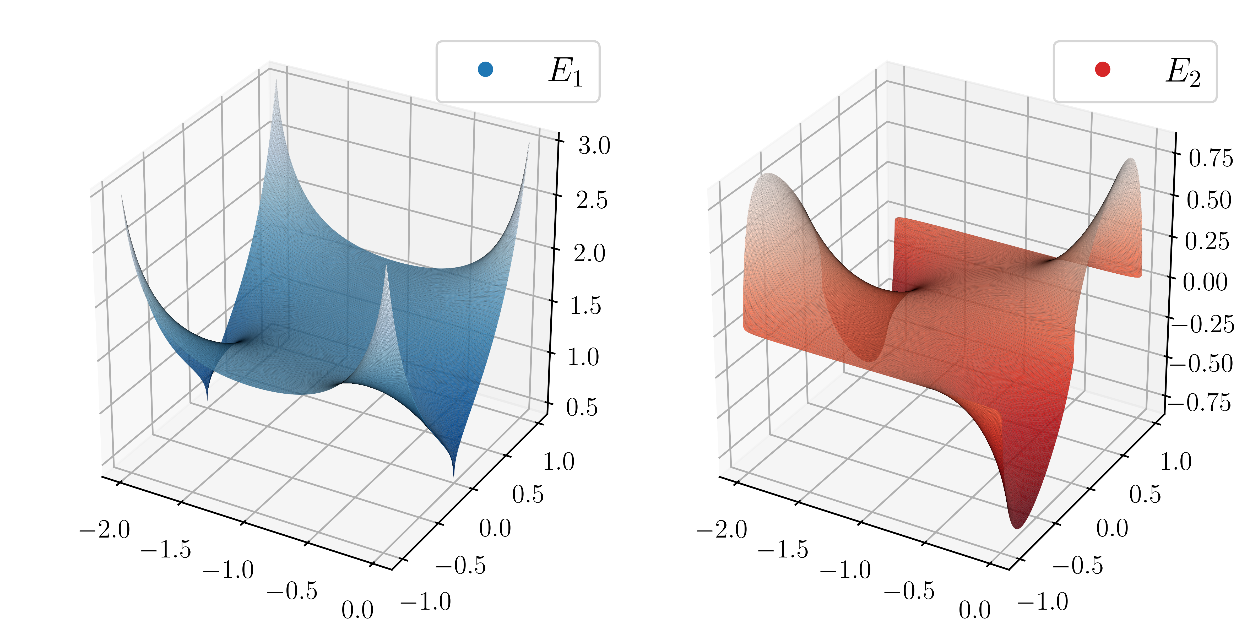
Figure 1: Plots of the first (blue/left) and the second (red/right) component of the numerically determined electric field.

These pictures indicate that ${\bf E}\in C^{0}(\overline{\Omega})$, or at least that ${\bf E}\in L^{\infty}(\Omega)$. In addition, (3.1) in conjunction with Weyl’s lemma imply that ${\bf E}\in C^{\infty}(\Omega)$. Note that since $E_{1}:={\bf E}\cdot{\bf e}_{1}={\bf E}_{0}\cdot{\bf e}_{1}$ on $\{0\}\times[-1,1]$, we find that ${{\bf E}\notin C^{0,\alpha}(\overline{\Omega})}$ for any ${\alpha\in\left(0,1\right]}$. Apart from that, if $\hat{p}\in\mathcal{P}^{\log}(\mathbb{R})$ is given via $\hat{p}(x):=1/\log(e+1/|x|)$ for all ${x\in\mathbb{R}}$, then it is easily checked that $p:=\hat{p}\circ|{\bf E}|^{2}$ satisfies ${p(0,x_{2})\log(e+1/|x_{2}|)\to\infty}$ as $x_{2}\to 0$ and, thus, $p\notin\mathcal{P}^{\log}(\Omega)$.

In the sequel, we do not use that ${\bf E}$ is the solution of the quasi-static Maxwell’s equations (LABEL:maxwell), but we will only use Assumption 3.3.

Theorem 3.6.

Let $\Omega\subseteq\mathbb{R}^{d}$, ${d\in\mathbb{N}}$, be open, $p\in\left[1,\infty\right)$ and let Assumption 3.3 be satisfied. Set $\smash{p^{*}:=\frac{dp}{d-p}}$ if $p<d$ and $p^{*}:=\infty$ if $p\geq d$. Then, for any open set $\Omega^{\prime}\subset\subset\Omega$ with ${\partial\Omega^{\prime}\in C^{0,1}}$ and any $\smash{\alpha\geq 1+\frac{2}{p}}$, it holds

$$\smash{X^{p,p}_{\nabla}(\Omega;|\mathbf{E}|^{2})\hookrightarrow L^{r}(\Omega^{\prime};|{\bf E}|^{\alpha r})}$$

with $r\in[1,p^{*}]$ if $p\neq d$ and $r\in[1,p^{*})$ if $p=d$.

• See [21, Thm. 3.3]. ∎

4 A weak stability lemma

The weak stability of problems of $p$–Laplace type is well-known (cf. [6]). It also holds for our problem (1.1) if we make appropriate natural assumptions on the extra stress tensor $\mathbf{S}$ and on the couple stress tensor $\mathbf{N}$, which are motivated by the canonical example in (1.3). We denote the symmetric and the skew-symmetric part, resp., of a tensor $\mathbf{A}\in\mathbb{R}^{d\times d}$ by ${\mathbf{A}^{{\mathrm{sym}}}:=\frac{1}{2}(\mathbf{A}+\mathbf{A}^{\top})}$ and ${\mathbf{A}^{{\mathrm{skew}}}:=\frac{1}{2}(\mathbf{A}-\mathbf{A}^{\top})}$. Moreover, ${\mathbb{R}^{d\times d}_{{\mathrm{sym}}}:=\{\mathbf{A}\in\mathbb{R}^{d\times d}\mid\mathbf{A}=\mathbf{A}^{\mathrm{sym}}\}}$ and $\mathbb{R}^{d\times d}_{{\mathrm{skew}}}:=\{\mathbf{A}\in\mathbb{R}^{d\times d}\mid{\mathbf{A}=\mathbf{A}^{\mathrm{skew}}}\}$.

Assumption 4.1.

For the extra stress tensor $\mathbf{S}:\mathbb{R}_{{\mathrm{sym}}}^{d\times d}\times\mathbb{R}_{{\mathrm{skew}}}^{d\times d}\times\mathbb{R}^{d}\to\mathbb{R}^{d}$ and some $\hat{p}\in\mathcal{P}^{\log}(\mathbb{R})$ with $\hat{p}^{-}>1$, there exist constants $c,C>0$ such that:

1. $\mathbf{S}\in C^{0}(\mathbb{R}_{{\mathrm{sym}}}^{d\times d}\times\mathbb{R}_{{\mathrm{skew}}}^{d\times d}\times\mathbb{R}^{d};\mathbb{R}^{d\times d})$.

2. For every ${\bf D}\in\mathbb{R}_{{\mathrm{sym}}}^{d\times d}$, ${\bf R}\in\mathbb{R}_{{\mathrm{skew}}}^{d\times d}$ and ${\bf E}\in\mathbb{R}^{d}$, it holds
   

   $$|\mathbf{S}^{{\mathrm{sym}}}(\mathbf{D},\mathbf{R},\mathbf{E})| \leq c\,\big{(}1+|\mathbf{E}|^{2}\big{)}\big{(}1+|\mathbf{D}|^{\hat{p}({\lvert{{\bf E}}\rvert}^{2})-1}\big{)}\,,$$

   $$|\mathbf{S}^{{\mathrm{skew}}}(\mathbf{D},\mathbf{R},\mathbf{E})| \leq c\,|\mathbf{E}|^{2}\big{(}1+|\mathbf{R}|^{\hat{p}({\lvert{{\bf E}}\rvert}^{2})-1}\big{)}\,.$$

   
   

3. For every ${\bf D}\in\mathbb{R}_{{\mathrm{sym}}}^{d\times d}$, ${\bf R}\in\mathbb{R}_{{\mathrm{skew}}}^{d\times d}$ and ${\bf E}\in\mathbb{R}^{d}$, it holds
   

   $$\mathbf{S}(\mathbf{D},\mathbf{R},\mathbf{E}):\mathbf{D} \geq c\,\big{(}1+|\mathbf{E}|^{2}\big{)}\,\big{(}|\mathbf{D}|^{\hat{p}({\lvert{{\bf E}}\rvert}^{2})}-C\big{)}\,,$$

   $$\mathbf{S}(\mathbf{D},\mathbf{R},\mathbf{E}):\mathbf{R} \geq c\,|\mathbf{E}|^{2}\big{(}|\mathbf{R}|^{\hat{p}({\lvert{{\bf E}}\rvert}^{2})}-C\big{)}\,.$$

   
   

4. For every ${\bf D}_{1},{\bf D}_{2}\in\mathbb{R}_{{\mathrm{sym}}}^{d\times d}$, ${\bf R}_{1},{\bf R}_{2}\in\mathbb{R}_{{\mathrm{skew}}}^{d\times d}$ and ${\bf E}\in\mathbb{R}^{d}$ with $(\mathbf{D}_{1},|\mathbf{E}|\mathbf{R}_{1})\neq(\mathbf{D}_{2},|\mathbf{E}|\mathbf{R}_{2})$, it holds
   

   $$\big{(}\mathbf{S}( \mathbf{D}_{1},\mathbf{R}_{1},\mathbf{E})-\mathbf{S}(\mathbf{D}_{2},\mathbf{R}_{2},\mathbf{E})\big{)}:\big{(}\mathbf{D}_{1}-\mathbf{D}_{2}+\mathbf{R}_{1}-\mathbf{R}_{2}\big{)}>0\,.$$

Assumption 4.2.

For the couple stress tensor $\mathbf{N}:\mathbb{R}^{d\times d}\times\mathbb{R}^{d}\to\mathbb{R}^{d\times d}$ and some $\hat{p}\in\mathcal{P}^{\log}(\mathbb{R})$ with $\hat{p}^{-}>1$, there exist constants $c,C>0$ such that:

1. $\mathbf{N}\in C^{0}(\mathbb{R}^{d\times d}\times\mathbb{R}^{d};\mathbb{R}^{d\times d})$.

2. For every ${\bf L}\in\mathbb{R}^{d\times d}$ and ${\bf E}\in\mathbb{R}^{d}$, it holds
   

   $$|\mathbf{N}(\mathbf{L},\mathbf{E})|\leq c\,\big{|}\mathbf{E}|^{2}\big{(}1+|\mathbf{L}|^{\hat{p}({\lvert{{\bf E}}\rvert}^{2})-1}\big{)}\,.$$

   
   

3. For every ${\bf L}\in\mathbb{R}^{d\times d}$ and ${\bf E}\in\mathbb{R}^{d}$, it holds
   

   $$\mathbf{N}(\mathbf{L},\mathbf{E}):\mathbf{L}\geq c\,\big{|}\mathbf{E}|^{2}\big{(}|\mathbf{L}|^{\hat{p}({\lvert{{\bf E}}\rvert}^{2})}-C\big{)}\,.$$

   
   

4. For every ${\bf L}_{1},{\bf L}_{2}\in\mathbb{R}^{d\times d}$ and ${\bf E}\in\mathbb{R}^{d}$ with $|\mathbf{E}|>0$ and $\mathbf{L}_{1}\neq\mathbf{L}_{2}$, it holds
   

   $$(\mathbf{N}(\mathbf{L}_{1},\mathbf{E})-\mathbf{N}(\mathbf{L}_{2},\mathbf{E})):(\mathbf{L}_{1}-\mathbf{L}_{2})>0\,.$$

Remark 4.3.

Let Assumption 3.3, Assumption 4.1 and Assumption 4.2 be satisfied. Since $|{\bf E}|^{2}\in W^{1,\infty}(\Omega^{\prime})$ for each $\Omega^{\prime}\subset\subset\Omega$, which follows from ${{\bf E}\in C^{\infty}(\Omega)}$, we have that the variable exponent

$$p:=\hat{p}\circ|{\bf E}|^{2}$$

satisfies $p\in\mathcal{P}^{\infty}(\Omega)\cap C^{0}(\Omega)$ and $p|_{\Omega^{\prime}}\in\mathcal{P}^{\log}(\Omega^{\prime})$ for each $\Omega^{\prime}\subset\subset\Omega$.

Lemma 4.4.

Let Assumption 3.3, Assumption 4.1 and Assumption 4.2 be satisfied with ${p^{-}\geq\frac{2d}{d+2}}$. Then, we have that $\smash{{\mathaccent 23{X}}^{p^{-},p(\cdot)}_{\mathbf{D}}(\Omega)\hookrightarrow W^{1,p(\cdot)}_{{\mathrm{loc}}}(\Omega)}$.

• Let $\Omega^{\prime}\subset\subset\Omega$ be arbitrary. Without loss of generality, we may assume that $\partial\Omega^{\prime}\in C^{0,1}$. Otherwise, we switch to some $\Omega^{\prime\prime}$ such that ${\Omega^{\prime}\subset\subset\Omega^{\prime\prime}\subset\subset\Omega}$ with ${\partial\Omega^{\prime\prime}\in C^{0,1}}$. Since $\smash{p\in C^{0}(\Omega)}$ (cf. Remark 4.3), Theorem 2.13 implies that any ${{\bf u}\in\smash{{\mathaccent 23{X}}^{p^{-},p(\cdot)}_{\mathbf{D}}(\Omega)}}$ satisfies ${\bf u}\in L^{p(\cdot)}(\Omega^{\prime})$ with

  $$\|{\bf u}\|_{L^{p(\cdot)}(\Omega^{\prime})}\leq c(p,\Omega^{\prime})\|{\bf u}\|_{\smash{{\mathaccent 23{X}}^{p^{-},p(\cdot)}_{\mathbf{D}}(\Omega)}}$$ (4.5)

  for some constant $c(p,\Omega^{\prime})\!>\!0$. Next, let $({\bf u}_{n})_{n\in\mathbb{N}}\!\subseteq\!\smash{\mathcal{V}^{p^{-},p(\cdot)}_{{\bf D}}}$ be a sequence such that ${\bf u}_{n}\to{\bf u}$ in $\smash{{\mathaccent 23{X}}^{p^{-},p(\cdot)}_{\mathbf{D}}(\Omega)}$ $(n\to\infty)$. Then, (4.5) gives us that ${\bf u}_{n}\to{\bf u}$ in $L^{p(\cdot)}(\Omega^{\prime})$ $(n\to\infty)$. In addition, since $\smash{p|_{\Omega^{\prime}}\in\mathcal{P}^{\log}(\Omega^{\prime})}$ (cf. Remark 4.3), Korn’s inequality (cf. Theorem 2.17 and $\smash{{\mathaccent 23{X}}^{p^{-},p(\cdot)}_{\mathbf{D}}(\Omega)}\hookrightarrow W^{1,p(\cdot)}(\Omega^{\prime})$) and (4.5) yield

  $$\|\nabla{\bf u}_{n}\|_{L^{p(\cdot)}(\Omega^{\prime})}+\|{\bf u}_{n}\|_{L^{p(\cdot)}(\Omega^{\prime})} \leq c(p,\Omega^{\prime})\big{(}\|{\bf D}{\bf u}_{n}\|_{L^{p(\cdot)}(\Omega^{\prime})}+\|{\bf u}_{n}\|_{L^{p(\cdot)}(\Omega^{\prime})}\big{)}$$

  $$\leq c(p,\Omega^{\prime})\|{\bf u}_{n}\|_{\smash{{\mathaccent 23{X}}^{p^{-},p(\cdot)}_{\mathbf{D}}(\Omega)}}\,.$$ (4.6)

  Thus, we observe that $({\bf u}_{n})_{n\in\mathbb{N}}\subseteq\smash{\mathcal{V}^{p^{-},p(\cdot)}_{{\bf D}}}$ is bounded in $W^{1,p(\cdot)}(\Omega^{\prime})$. This implies the existence of a vector field $\tilde{\bf u}\in W^{1,p(\cdot)}(\Omega^{\prime})$ and of a not relabeled subsequence such that ${\bf u}_{n}\rightharpoonup\tilde{\bf u}$ in $W^{1,p(\cdot)}(\Omega^{\prime})$ $(n\to\infty)$. Due to the uniqueness of weak limits, we conclude that ${\bf u}=\tilde{\bf u}$ in $W^{1,p(\cdot)}(\Omega^{\prime})$ and by taking the limit inferior in (4.6) that $\|{\bf u}\|_{W^{1,p(\cdot)}(\Omega^{\prime})}\leq c(p,\Omega^{\prime})\|{\bf u}\|_{\smash{{\mathaccent 23{X}}^{p^{-},p(\cdot)}_{\mathbf{D}}(\Omega)}}$. ∎

  Lemma 4.7.

  Let Assumption 3.3, Assumption 4.1 and Assumption 4.2 be satisfied with ${p^{-}\geq\frac{2d}{d+2}}$. Then, we have that $\smash{{\mathaccent 23{X}}^{p^{-},p(\cdot)}_{{\nabla}}(\Omega;|\mathbf{E}|^{2})\hookrightarrow W^{1,p(\cdot)}_{{\mathrm{loc}}}(\Omega_{0})}$ and $\smash{\nabla({\bf w}|_{\Omega^{\prime}})=(\hat{\nabla}{\bf w})|_{\Omega^{\prime}}}$ for all ${{\bf w}\in\smash{{\mathaccent 23{X}}^{p^{-},p(\cdot)}_{{\nabla}}(\Omega;|\mathbf{E}|^{2})}}$ and $\Omega^{\prime}\subset\subset\Omega_{0}$.

• Let $\Omega^{\prime}\subset\subset\Omega_{0}$ be arbitrary and fix some $\Omega^{\prime\prime}\subset\subset\Omega_{0}$ such that $\Omega^{\prime}\subset\subset\Omega^{\prime\prime}$. Due to ${|{\bf E}|>0}$ in $\overline{\Omega^{\prime\prime}}$ and ${|{\bf E}|\in C^{0}(\overline{\Omega^{\prime\prime}})}$, there is a constant $c(\Omega^{\prime\prime})>0$ such that $c(\Omega^{\prime\prime})\leq|{\bf E}|^{2}$ in $\overline{\Omega^{\prime\prime}}$. Thus, for every ${\bf w}\in C_{0}^{\infty}(\Omega)$, Hölder’s inequality in variable Lebesgue spaces and (2.1) imply

  $$\|{\bf w}\|_{{X^{p^{-},p(\cdot)}_{{\nabla}}(\Omega^{\prime\prime})}}\leq 2\,\smash{c(\Omega^{\prime\prime})^{\frac{-1}{p^{-}}}\|{\bf w}\|_{{{\mathaccent 23{X}}^{p^{-},p(\cdot)}_{{\nabla}}(\Omega;|\mathbf{E}|^{2})}}\,.}$$ (4.8)

  Furthermore, since $p|_{\Omega^{\prime\prime}}\in C^{0}(\Omega^{\prime\prime})$ (cf. Remark 4.3) and $p^{-}\geq\frac{2d}{d+2}$, Theorem 2.13 implies that every ${\bf w}\in C_{0}^{\infty}(\Omega)$ satisfies

  $$\|{\bf w}\|_{L^{p(\cdot)}(\Omega^{\prime})}\leq c(p,\Omega^{\prime},\Omega^{\prime\prime})\|{\bf w}\|_{{X^{p^{-},p(\cdot)}_{{{\bf D}}}(\Omega^{\prime\prime})}}\leq c(p,\Omega^{\prime},\Omega^{\prime\prime})\|{\bf w}\|_{{X^{p^{-},p(\cdot)}_{{\nabla}}(\Omega^{\prime\prime})}}$$ (4.9)

  for some constant $c(p,\Omega^{\prime},\Omega^{\prime\prime})>0$. Combining (4.8) and (4.9), we find that for every ${\bf w}\in C_{0}^{\infty}(\Omega)$, it holds

  $$\|{\bf w}\|_{W^{1,p(\cdot)}(\Omega^{\prime})}\leq c(p,\Omega^{\prime},\Omega^{\prime\prime})\|{\bf w}\|_{{{\mathaccent 23{X}}^{p^{-},p(\cdot)}_{{\nabla}}(\Omega;|\mathbf{E}|^{2})}}$$ (4.10)

  for some constant $c(p,\Omega^{\prime},\Omega^{\prime\prime})\!>\!0$. Since $\smash{{\mathaccent 23{X}}^{p^{-},p(\cdot)}_{{\nabla}}(\Omega;|\mathbf{E}|^{2})}$ is the closure of $\smash{C_{0}^{\infty}(\Omega)}$, and $C^{\infty}(\overline{\Omega^{\prime}})$ is dense in $W^{1,p(\cdot)}(\Omega^{\prime})$ (cf. [5, Thm. 9.1.7]) since $p|_{\Omega^{\prime\prime}}\in\mathcal{P}^{\log}(\Omega^{\prime\prime})$ (cf. Remark 4.3), (4.10) implies $\smash{{\mathaccent 23{X}}^{p^{-},p(\cdot)}_{{\nabla}}(\Omega;|\mathbf{E}|^{2})\hookrightarrow W^{1,p(\cdot)}(\Omega^{\prime})}$ and $\smash{\nabla}({\bf w}|_{\Omega^{\prime}})=(\hat{\nabla}{\bf w})|_{\Omega^{\prime}}$ for every ${{\bf w}\in\smash{{\mathaccent 23{X}}^{p^{-},p(\cdot)}_{{\nabla}}(\Omega;|\mathbf{E}|^{2})}}$. ∎

  Now we can formulate the following weak stability property for problem (1.1).

  Lemma 4.11.

  Let $\Omega\subseteq\mathbb{R}^{d}$, $d\geq 2$, be a bounded domain and let Assumption 3.3, Assumption 4.1 and Assumption 4.2 be satisfied with ${p^{-}>\frac{2d}{d+2}}$. Moreover, let $\smash{({\bf v}^{n})_{n\in\mathbb{N}}\subseteq{\mathaccent 23{X}}^{p^{-},p(\cdot)}_{\mathbf{D},\operatorname{div}}(\Omega)}$ and $\smash{(\boldsymbol{\omega}^{n})_{n\in\mathbb{N}}\subseteq{\mathaccent 23{X}}^{p^{-},p(\cdot)}_{{\nabla}}(\Omega;|\mathbf{E}|^{2})}$ be such that $({\bf R}({\bf v}^{n},\boldsymbol{\omega}^{n}))_{n\in\mathbb{N}}\subseteq L^{p(\cdot)}(\Omega;|{\bf E}|^{2})$ is bounded and

  $$\begin{aligned} {\bf v}^{n}&\rightharpoonup{\bf v}\quad&&\text{in}\ {\mathaccent 23{X}}^{p^{-},p(\cdot)}_{\mathbf{D},\operatorname{div}}(\Omega)&&\quad(n\to\infty)\,,\\ \boldsymbol{\omega}^{n}&\rightharpoonup\boldsymbol{\omega}\quad&&\text{in}\ {\mathaccent 23{X}}^{p^{-},p(\cdot)}_{{\nabla}}(\Omega;|\mathbf{E}|^{2})&&\quad(n\to\infty)\,.\end{aligned}$$ (4.12)

  For every ball ${B\subset\subset\Omega_{0}}$ such that ${B^{\prime}:=2B\subset\subset\Omega_{0}}$ and $\tau\in C_{0}^{\infty}(B^{\prime})$ satisfying ${\chi_{B}\leq\tau\leq\chi_{B^{\prime}}}$, we set ${\mathbf{u}^{n}:=(\mathbf{v}^{n}-\mathbf{v})\tau}$, ${{\boldsymbol{\psi}}^{n}:=(\boldsymbol{\omega}^{n}-\boldsymbol{\omega})\tau}\in W^{1,p(\cdot)}_{0}(B^{\prime})$, $n\in\mathbb{N}$. Let $\mathbf{u}^{n,j}\in W^{1,\infty}_{0}(B^{\prime})$, $n,j\in\mathbb{N}$, and ${\boldsymbol{\psi}}^{n,j}\in W^{1,\infty}_{0}(B^{\prime})$, $n,j\in\mathbb{N}$, resp., denote the Lipschitz truncations constructed according to Theorem 2.18. Furthermore, assume that for every ${j\in\mathbb{N}}$, we have that

  $$\limsup_{n\to\infty}\big{|}\big{\langle} \mathbf{S}\big{(}\mathbf{D}\mathbf{v}^{n},\mathbf{R}(\mathbf{v}^{n},\boldsymbol{\omega}^{n}),\mathbf{E}\big{)}-\mathbf{S}\big{(}\mathbf{D}\mathbf{v},\mathbf{R}(\mathbf{v},\boldsymbol{\omega}),\mathbf{E}\big{)},\mathbf{D}{\bf u}^{n,j}+\mathbf{R}({\bf u}^{n,j},{\boldsymbol{\psi}}^{n,j})\big{\rangle}$$

  $$\quad+\big{\langle}\mathbf{N}(\nabla\boldsymbol{\omega}^{n},\mathbf{E})-\mathbf{N}(\nabla\boldsymbol{\omega},\mathbf{E}),\nabla{\boldsymbol{\psi}}^{n,j}\big{\rangle}\big{|}\leq\delta_{j}\,,$$ (4.13)

  where $\delta_{j}\to 0$ $(j\to 0)$. ​Then, ​one has $\nabla{\bf v}^{n}\to\nabla{\bf v}$ a.e. in $B$ ${(n\to\infty)}$, ${\nabla\boldsymbol{\omega}^{n}\to\nabla\boldsymbol{\omega}}$ a.e. in $B$ $(n\to\infty)$ and $\boldsymbol{\omega}^{n}\to\boldsymbol{\omega}$ a.e. in $B$ $(n\to\infty)$ for a suitable subsequence.

Remark 4.14.

(i) For each ball $B^{\prime}\subset\subset\Omega_{0}$, Lemma 4.4 and Lemma 4.7 yield the embeddings $\smash{{\mathaccent 23{X}}^{p^{-},p(\cdot)}_{\mathbf{D}}(\Omega)},\smash{{\mathaccent 23{X}}^{p^{-},p(\cdot)}_{{\nabla}}(\Omega;|\mathbf{E}|^{2})}\hookrightarrow\smash{W^{1,p(\cdot)}(B^{\prime})}$ and, therefore, that ${{\bf v}^{n}-{\bf v},\boldsymbol{\omega}^{n}-\boldsymbol{\omega}\!\in\!W^{1,p(\cdot)}(B^{\prime})}$ for all $n\!\in\!\mathbb{N}$, which is crucial for the applicability of the Lipschitz truncation technique (cf. Theorem 2.18). In particular, Lemma 4.7 yields that ${\nabla(\boldsymbol{\omega}|_{B^{\prime}})=(\hat{\nabla}\boldsymbol{\omega})|_{B^{\prime}}}$ in $L^{p(\cdot)}(B^{\prime})$ for all $\boldsymbol{\omega}\in\smash{{\mathaccent 23{X}}^{p^{-},p(\cdot)}_{{\nabla}}(\Omega;|\mathbf{E}|^{2})}$, which is precisely the sense in which the gradients of both $\boldsymbol{\omega}\in\smash{{\mathaccent 23{X}}^{p^{-},p(\cdot)}_{{\nabla}}(\Omega;|\mathbf{E}|^{2})}$ and ${(\boldsymbol{\omega}^{n})_{n\in\mathbb{N}}\in\smash{{\mathaccent 23{X}}^{p^{-},p(\cdot)}_{{\nabla}}(\Omega;|\mathbf{E}|^{2})}}$ are to be understood in (4.13).

(ii) The boundedness of $({\bf R}({\bf v}^{n},\boldsymbol{\omega}^{n}))_{n\in\mathbb{N}}\subseteq L^{p(\cdot)}(\Omega;|{\bf E}|^{2})$ yields a tensor field $\widehat{{\bf R}}\in L^{p(\cdot)}(\Omega;|{\bf E}|^{2})$ such that up to a not relabeled subsequence

$${\bf R}({\bf v}^{n},\boldsymbol{\omega}^{n})\rightharpoonup\widehat{{\bf R}}\quad\text{in}\ L^{p(\cdot)}(\Omega;|{\bf E}|^{2})\quad(n\to\infty)\,.$$ (4.15)

Using the embedding $L^{p(\cdot)}(\Omega)\hookrightarrow L^{p^{-}}(\Omega)$, Korn’s inequality for the constant exponent $p^{-}\geq\frac{2d}{d+2}$ and $L^{p^{-}}(\Omega)\hookrightarrow L^{p^{-}}(\Omega;{\lvert{{\bf E}}\rvert}^{2})$, since ${{\bf E}\in L^{\infty}(\Omega)}$, we deduce from (4.12) that

$$\begin{aligned} \nabla{\bf v}^{n}&\rightharpoonup\nabla{\bf v}\quad&&\text{in}\ L^{p^{-}}(\Omega;|{\bf E}|^{2})&&\quad(n\to\infty)\,,\\ \boldsymbol{\omega}^{n}\cdot\boldsymbol{\varepsilon}&\rightharpoonup\boldsymbol{\omega}\cdot\boldsymbol{\varepsilon}\quad&&\text{in}\ L^{p^{-}}(\Omega;|{\bf E}|^{2})&&\quad(n\to\infty)\,.\end{aligned}$$ (4.16)

Combining (4.15), (4.16), the embedding $L^{p(\cdot)}(\Omega;{\lvert{{\bf E}}\rvert}^{2})\hookrightarrow L^{p^{-}}(\Omega;{\lvert{{\bf E}}\rvert}^{2})$ and the definition of ${\bf R}({\bf v},\boldsymbol{\omega})$, we conclude that ${\bf R}({\bf v},\boldsymbol{\omega})=\widehat{{\bf R}}\in L^{p(\cdot)}(\Omega;|{\bf E}|^{2})$ in (4.15). Thus, the expression with ${\bf R}({\bf v},\boldsymbol{\omega})$ in (4.13) is well-defined.

• In view of the embeddings $\smash{{\mathaccent 23{X}}^{p^{-},p(\cdot)}_{\mathbf{D},\operatorname{div}}(\Omega)\hookrightarrow W^{1,p(\cdot)}(B^{\prime})}$, $\smash{{\mathaccent 23{X}}^{p^{-},p(\cdot)}_{{\nabla}}(\Omega;|\mathbf{E}|^{2})\hookrightarrow W^{1,p(\cdot)}(B^{\prime})}$ (cf. Lemma 4.4 and Lemma 4.7) as well as $W^{1,p(\cdot)}(B^{\prime})\hookrightarrow W^{1,p^{-}}(B^{\prime})$, we deduce from (4.12), also using Rellich’s compact-ness theorem for constant exponents and Theorem 2.16, that

  $$\begin{aligned} {\bf v}^{n}&\rightharpoonup{\bf v}\quad&&\text{in}\ W^{1,p(\cdot)}(B^{\prime})&&\quad(n\to\infty)\,,\\ {\bf v}^{n}&\to{\bf v}\quad&&\text{in}\ L^{q}(B^{\prime})\cap L^{p(\cdot)}(B^{\prime})\text{ and a.e. in }B^{\prime}&&\quad(n\to\infty)\,,\\ \boldsymbol{\omega}^{n}&\rightharpoonup\boldsymbol{\omega}\quad&&\text{in}\ W^{1,p(\cdot)}(B^{\prime})&&\quad(n\to\infty)\,,\\ \boldsymbol{\omega}^{n}&\to\boldsymbol{\omega}\quad&&\text{in}\ L^{q}(B^{\prime})\cap L^{p(\cdot)}(B^{\prime})\text{ and a.e. in }B^{\prime}&&\quad(n\to\infty)\,,\end{aligned}$$ (4.17)

  where $q\in\left[1,(p^{-})^{*}\right)$. ​Throughout the proof, we will employ the particular notation

  $$\begin{aligned} \widetilde{\bf S}&:=\mathbf{S}\big{(}\mathbf{D}\mathbf{v},\mathbf{R}(\mathbf{v},\boldsymbol{\omega}),\mathbf{E}\big{)}\,,\quad&&\mathbf{S}^{n}\,:=\mathbf{S}\big{(}\mathbf{D}\mathbf{v}^{n},\mathbf{R}(\mathbf{v}^{n},\boldsymbol{\omega}^{n}),\mathbf{E}\big{)}\,,\\ \widetilde{\bf N}&:=\mathbf{N}(\nabla\boldsymbol{\omega},\mathbf{E})\,,\quad&&\mathbf{N}^{n}:=\mathbf{N}(\nabla\boldsymbol{\omega}^{n},\mathbf{E})\,.\end{aligned}$$ (4.18)

  Using (S.2), (N.2), Assumption 3.3, (4.12) and Remark 4.14, we obtain a constant ${K:=K({\bf E})>0}$ (not depending on $n\in\mathbb{N}$) such that

  $$\|{\bf v}^{n}\|_{\smash{{\mathaccent 23{X}}^{p^{-},p(\cdot)}_{\mathbf{D},\operatorname{div}}(\Omega)}}\!+\|{\bf v}\|_{\smash{{\mathaccent 23{X}}^{p^{-},p(\cdot)}_{\mathbf{D},\operatorname{div}}(\Omega)}}\!+\|\boldsymbol{\omega}^{n}\|_{p^{-},p(\cdot),{\lvert{{\bf E}}\rvert}^{2}}\!+\|\boldsymbol{\omega}\|_{p^{-},p(\cdot),{\lvert{{\bf E}}\rvert}^{2}} \leq K\,,$$ (4.19)

  $$\|{\bf R}({\bf v}^{n},\boldsymbol{\omega}^{n})\|_{p(\cdot),{\lvert{{\bf E}}\rvert}^{2}}+\|{\bf R}({\bf v},\boldsymbol{\omega})\|_{p(\cdot),{\lvert{{\bf E}}\rvert}^{2}} \leq K\,,$$

  $$\|\mathbf{S}^{n}\|_{p^{\prime}(\cdot)}\!+\|\widetilde{\mathbf{S}}\|_{p^{\prime}(\cdot)}\!+\|(\mathbf{S}^{n})^{\mathrm{skew}}\|_{\smash{p^{\prime}(\cdot),|{\bf E}|^{\smash{\frac{-2}{p(\cdot)-1}}}}}\!+\|\widetilde{\mathbf{S}}^{\mathrm{skew}}\|_{\smash{p^{\prime}(\cdot),|{\bf E}|^{\smash{\frac{-2}{p(\cdot)-1}}}}} \leq K\,,$$

  $$\|\mathbf{N}^{n}\|_{\smash{p^{\prime}(\cdot),|{\bf E}|^{\smash{\frac{-2}{p(\cdot)-1}}}}}+\|\widetilde{\mathbf{N}}\|_{\smash{p^{\prime}(\cdot),|{\bf E}|^{\smash{\frac{-2}{p(\cdot)-1}}}}} \leq K\,.$$

  Recall that $\tau\in C_{0}^{\infty}(B^{\prime})$ with $\chi_{B}\leq\tau\leq\chi_{B^{\prime}}$. Hence, using (S.4) and (N.4), we get

  $$I^{n}\!:=\!\int_{B}\!\big{[}\!\big{(}{\bf S}^{n}\!-\!\widetilde{\bf S}\big{)}\!:\!\big{(}\mathbf{D}({\bf v}^{n}\!-\!{\bf v})\!+\!\mathbf{R}({\bf v}^{n}\!-\!{\bf v},\boldsymbol{\omega}^{n}\!-\!\boldsymbol{\omega})\big{)}\!+\!\big{(}{\bf N}^{n}\!-\!\widetilde{\bf N}\big{)}\!:\!\nabla(\boldsymbol{\omega}^{n}\!-\!\boldsymbol{\omega})\big{)}^{\theta}\,dx$$

  $$\leq\!\int_{B^{\prime}}\!\big{[}\big{(}{\bf S}^{n}\!-\!\widetilde{\bf S}\big{)}\!:\!\big{(}\mathbf{D}({\bf v}^{n}\!-\!{\bf v})\!+\!\mathbf{R}({\bf v}^{n}\!-\!{\bf v},\boldsymbol{\omega}^{n}\!-\!\boldsymbol{\omega})\big{)}\!+\!\big{(}{\bf N}^{n}\!-\!\widetilde{\bf N}\big{)}\!:\!\nabla(\boldsymbol{\omega}^{n}\!-\!\boldsymbol{\omega})\big{)}^{\theta}\!\tau^{\theta}\,dx$$

  $$\leq\int_{B^{\prime}}\big{[}\big{(}{\bf S}^{n}-\widetilde{\bf S}\big{)}:\big{(}\mathbf{D}({\bf v}^{n}-{\bf v})+\mathbf{R}({\bf v}^{n}-{\bf v},\boldsymbol{\omega}^{n}-\boldsymbol{\omega})\big{)}\tau\big{)}^{\theta}\,dx$$ (4.20)

  $$\quad+\int_{B^{\prime}}\big{[}\big{(}{\bf N}^{n}-\widetilde{\bf N}\big{)}:\nabla(\boldsymbol{\omega}^{n}-\boldsymbol{\omega})\tau\big{)}^{\theta}dx=:\int_{B^{\prime}}\alpha_{n}^{\theta}\,dx+\int_{B^{\prime}}\beta_{n}^{\theta}\,dx\,,$$

  where we also used that

  $$\smash{\frac{1}{2}}(a^{\theta}+b^{\theta})\leq(a+b)^{\theta}\leq a^{\theta}+b^{\theta}$$ (4.21)

  valid for all $a,b\geq 0$ and ${\theta\in(0,1)}$. Then, splitting the integral of $\alpha_{n}^{\theta}$ over $B^{\prime}$ into an integral over $\{\mathbf{u}^{n}\neq\mathbf{u}^{n,j}\}$ and one over $\{\mathbf{u}^{n}=\mathbf{u}^{n,j}\}$, also using Hölder’s inequality with exponents $\frac{1}{\theta},\frac{1}{1-\theta}$, we find that

  $$\int_{B^{\prime}}\alpha_{n}^{\theta}\,dx \leq\|\alpha_{n}\|_{L^{1}(B^{\prime})}^{\theta}|\{\mathbf{u}^{n}\neq\mathbf{u}^{n,j}\}|^{1-\theta}+\|\alpha_{n}\chi_{\{\mathbf{u}^{n}=\mathbf{u}^{n,j}\}}\|_{L^{1}(B^{\prime})}^{\theta}|B^{\prime}|^{1-\theta}$$

  $$=:(I_{1}^{n})^{\theta}|\{\mathbf{u}^{n}\neq\mathbf{u}^{n,j}\}|^{1-\theta}+\|\alpha_{n}\chi_{\{\mathbf{u}^{n}=\mathbf{u}^{n,j}\}}\|_{L^{1}(B^{\prime})}^{\theta}|B^{\prime}|^{1-\theta}\,.$$ (4.22)

  For the first term, we will use (2.19)₄ and, thus, have to show that $(I_{1}^{n})_{n\in\mathbb{R}}\subseteq\mathbb{R}$ is bounded. In fact, by combining (4.12), (4.19), $\tau\leq 1$, as well as

  $${\bf A}:({\bf D}{\bf u}+{\bf R}({\bf u},{\bf w}))={\bf A}:\nabla{\bf u}+{\bf A}^{\mathrm{skew}}:({\boldsymbol{\varepsilon}}\cdot{\bf w})\,,$$ (4.23)

  valid for vector fields ${\bf u}$, ${\bf w}$ and tensor fields ${\bf A}$, we observe that

  $$\begin{aligned} I_{1}^{n}&\leq\big{(}\|({\bf S}^{n})^{\mathrm{sym}}\|_{p^{\prime}(\cdot)}+\|\widetilde{\bf S}^{\mathrm{sym}}\|_{p^{\prime}(\cdot)}\big{)}\|{\bf D}{\bf v}^{n}-{\bf D}{\bf v}\|_{p(\cdot)}\\ &\quad+\big{(}\|({\bf S}^{n})^{\mathrm{skew}}\|_{\smash{p^{\prime}(\cdot),|{\bf E}|^{\smash{\frac{-2}{p(\cdot)-1}}}}}+\|\widetilde{\bf S}^{\mathrm{skew}}\|_{\smash{p^{\prime}(\cdot),|{\bf E}|^{\smash{\frac{-2}{p(\cdot)-1}}}}}\big{)}\times\\ &\qquad\quad\times\|{\bf R}({\bf v}^{n},\boldsymbol{\omega}^{n})-{\bf R}({\bf v},\boldsymbol{\omega})\|_{p(\cdot),{\lvert{{\bf E}}\rvert}^{2}}\leq 2\,K^{2}\,.\end{aligned}$$ (4.24)

  Similarly, we deduce that

  $$\int_{B^{\prime}}\beta_{n}^{\theta}\,dx \leq\|\beta_{n}\|_{L^{1}(B^{\prime})}^{\theta}|\{{\boldsymbol{\psi}}^{n}\neq{\boldsymbol{\psi}}^{n,j}\}|^{1-\theta}+\|\beta_{n}\chi_{\{{\boldsymbol{\psi}}^{n}={\boldsymbol{\psi}}^{n,j}\}}\|_{L^{1}(B^{\prime})}^{\theta}|B^{\prime}|^{1-\theta}$$

  $$=:(I_{2}^{n})^{\theta}|\{{\boldsymbol{\psi}}^{n}\neq{\boldsymbol{\psi}}^{n,j}\}|^{1-\theta}+\|\beta_{n}\chi_{\{{\boldsymbol{\psi}}^{n}={\boldsymbol{\psi}}^{n,j}\}}\|_{L^{1}(B^{\prime})}^{\theta}|B^{\prime}|^{1-\theta}\,,$$ (4.25)

  and that

  $$\begin{aligned} I_{2}^{n}&\leq\big{(}\|{\bf N}^{n}\|_{\smash{p^{\prime}(\cdot),|{\bf E}|^{\smash{\frac{-2}{p(\cdot)-1}}}}}+\|\widetilde{\bf N}\|_{\smash{p^{\prime}(\cdot),|{\bf E}|^{\smash{\frac{-2}{p(\cdot)-1}}}}}\big{)}\|\nabla\boldsymbol{\omega}^{n}-\nabla\boldsymbol{\omega}\|_{p(\cdot),{\lvert{{\bf E}}\rvert}^{2}}\leq K^{2}\,.\end{aligned}$$ (4.26)

  Using (4.22), (4.24)–(4.26) and (4.21) we, thus, conclude that

  $$\begin{aligned} &\int_{B^{\prime}}\alpha_{n}^{\theta}\,dx+\int_{B^{\prime}}\beta_{n}^{\theta}\,dx\\ &\leq 2^{\theta}K^{2\theta}\big{(}|\{{\bf u}^{n}\neq{\bf u}^{n,j}\}|^{1-\theta}+|\{{\boldsymbol{\psi}}^{n}\neq{\boldsymbol{\psi}}^{n,j}\}|^{1-\theta}\big{)}\\ &\quad+2\,|B^{\prime}|^{1-\theta}\,\bigg{(}\int_{B^{\prime}}{\alpha_{n}\chi_{\{{\bf u}^{n}={\bf u}^{n,j}\}}\,dx}+\int_{B^{\prime}}{\beta_{n}\,\chi_{\{{\boldsymbol{\psi}}^{n}={\boldsymbol{\psi}}^{n,j}\}}\,dx}\bigg{)}^{\smash{\theta}}\,.\end{aligned}$$ (4.27)

  Let us now treat the last two integrals, which we denote by $I_{3}^{n,j}$ and $I_{4}^{n,j}$. We have that $\nabla({\bf v}^{n}-{\bf v})\tau=\nabla{\bf u}^{n,j}-({\bf v}^{n}-{\bf v})\otimes\nabla\tau$ on $\{\mathbf{u}^{n}=\mathbf{u}^{n,j}\}$, which, using (4.23), implies that

  $$\begin{aligned} I_{3}^{n,j}&={\big{\langle}{{\bf S}^{n}-\widetilde{\bf S}},{\big{(}\nabla{\bf u}^{n,j}-({\bf v}^{n}-{\bf v})\otimes\nabla\tau\big{)}\chi_{\{\mathbf{u}^{n}=\mathbf{u}^{n,j}\}}}\big{\rangle}}\\ &\quad+{\big{\langle}{\big{(}{\bf S}^{n}-\widetilde{\bf S}\big{)}^{\mathrm{skew}}},{{\boldsymbol{\varepsilon}}\cdot{\boldsymbol{\psi}}^{n,j}\chi_{\{{\boldsymbol{\psi}}^{n}={\boldsymbol{\psi}}^{n,j}\}}}\big{\rangle}}\\ &\quad+{\big{\langle}{\big{(}{\bf S}^{n}-\widetilde{\bf S}\big{)}^{\mathrm{skew}}},{{\boldsymbol{\varepsilon}}\cdot(\boldsymbol{\omega}^{n}-\boldsymbol{\omega})\tau\chi_{\{\mathbf{u}^{n}=\mathbf{u}^{n,j}\}\cap\{{\boldsymbol{\psi}}^{n}\neq{\boldsymbol{\psi}}^{n,j}\}}}\big{\rangle}}\\ &\quad-{\big{\langle}{\big{(}{\bf S}^{n}-\widetilde{\bf S}\big{)}^{\mathrm{skew}}},{{\boldsymbol{\varepsilon}}\cdot(\boldsymbol{\omega}^{n}-\boldsymbol{\omega})\tau\chi_{\{\mathbf{u}^{n}\neq\mathbf{u}^{n,j}\}\cap\{{\boldsymbol{\psi}}^{n}={\boldsymbol{\psi}}^{n,j}\}}}\big{\rangle}}\,.\end{aligned}$$ (4.28)

  We have $\nabla(\boldsymbol{\omega}^{n}-\boldsymbol{\omega})\tau=\nabla{\boldsymbol{\psi}}^{n,j}-(\boldsymbol{\omega}^{n}-\boldsymbol{\omega})\otimes\nabla\tau$ on $\{{\boldsymbol{\psi}}^{n}={\boldsymbol{\psi}}^{n,j}\}$, which implies that

  $$\begin{aligned} I_{4}^{n,j}={\big{\langle}{{\bf N}^{n}-\widetilde{\bf N}},{\big{(}\nabla{\boldsymbol{\psi}}^{n,j}-(\boldsymbol{\omega}^{n}-\boldsymbol{\omega})\otimes\nabla\tau\big{)}\chi_{\{{\boldsymbol{\psi}}^{n}={\boldsymbol{\psi}}^{n,j}\}}}\big{\rangle}}\,.\end{aligned}$$ (4.29)

  Using (4.23) and adding suitable terms, we deduce from (4.28) and (4.29) that

  $$\begin{aligned} I^{n,j}_{3}+I^{n,j}_{4}&\leq{\big{\lvert}{{\big{\langle}{{\bf S}^{n}-\widetilde{\bf S}},{{\bf D}{\bf u}^{n,j}+\mathbf{R}({\bf u}^{n,j},{\boldsymbol{\psi}}^{n,j})}\big{\rangle}}+{\big{\langle}{{\bf N}^{n}-\widetilde{\bf N}},{\nabla{\boldsymbol{\psi}}^{n,j}}\big{\rangle}}}\big{\rvert}}\\ &\quad+{\big{\lvert}{{\big{\langle}{{\bf S}^{n}-\widetilde{\bf S}},{\!\nabla{\bf u}^{n,j}\chi_{\{\mathbf{u}^{n}\neq\mathbf{u}^{n,j}\}}}\big{\rangle}}}\big{\rvert}}\\ &\quad+{\big{\lvert}{{\big{\langle}{{\bf N}^{n}-\widetilde{\bf N}},{\nabla{\boldsymbol{\psi}}^{n,j}\chi_{\{{\boldsymbol{\psi}}^{n}\neq{\boldsymbol{\psi}}^{n,j}\}}}\big{\rangle}}}\big{\rvert}}\\ &\quad+{\big{\lvert}{{\big{\langle}{\big{(}{\bf S}^{n}-\widetilde{\bf S}\big{)}^{\mathrm{skew}}},{{\boldsymbol{\varepsilon}}\cdot{\boldsymbol{\psi}}^{n,j}\chi_{\{{\boldsymbol{\psi}}^{n}\neq{\boldsymbol{\psi}}^{n,j}\}}}\big{\rangle}}}\big{\rvert}}\\ &\quad+{\big{\langle}{{\big{\lvert}{\big{(}{\bf S}^{n}-\widetilde{\bf S}\big{)}^{\mathrm{skew}}}\big{\rvert}}},{{\big{\lvert}{\boldsymbol{\omega}^{n}-\boldsymbol{\omega}}\big{\rvert}}\tau}\big{\rangle}}\\ &\quad+{\big{\langle}{{\big{\lvert}{({\bf S}^{n}-\widetilde{\bf S})^{\mathrm{sym}}}\big{\rvert}}},{{\big{\lvert}{(({\bf v}^{n}-{\bf v})\otimes\nabla\tau)^{\mathrm{sym}}}\big{\rvert}}}\big{\rangle}}\\ &\quad+{\big{\langle}{{\big{\lvert}{{\bf N}^{n}-\widetilde{\bf N}}\big{\rvert}}},{{\big{\lvert}{(\boldsymbol{\omega}^{n}-\boldsymbol{\omega})\otimes\nabla\tau}\big{\rvert}}}\big{\rangle}}\\ &=:I_{5}^{n,j}+I_{6}^{n,j}+I_{7}^{n,j}+I_{8}^{n,j}+I_{9}^{n,j}+I_{10}^{n,j}+I_{11}^{n,j}\,.\end{aligned}$$ (4.30)

  The term $I_{5}^{n,j}\!$, i.e., the first line on the right-hand side in (4.30), is handled by (4.13). For the other terms we obtain, using Hölder’s inequality, (2.1) and (4.19),

  $$I_{6}^{n,j} \leq 2\,\big{(}\|{\bf S}^{n}\|_{p^{\prime}(\cdot)}+\|\widetilde{\bf S}\|_{p^{\prime}(\cdot)}\big{)}\|\nabla{\bf u}^{n,j}\chi_{\{\mathbf{u}^{n}\neq\mathbf{u}^{n,j}\}}\|_{L^{p(\cdot)}(B^{\prime})}$$

  $$\leq 2\,K\|\nabla{\bf u}^{n,j}\chi_{\{\mathbf{u}^{n}\neq\mathbf{u}^{n,j}\}}\|_{L^{p(\cdot)}(B^{\prime})}\,,$$ (4.31)

  $$I_{7}^{n,j} \leq 2\,\big{(}\|{\bf N}^{n}\|_{\smash{p^{\prime}(\cdot),|{\bf E}|^{\smash{\frac{-2}{p(\cdot)-1}}}}}+\|\widetilde{\bf N}\|_{\smash{p^{\prime}(\cdot),|{\bf E}|^{\smash{\frac{-2}{p(\cdot)-1}}}}}\big{)}\|\nabla{\boldsymbol{\psi}}^{n,j}\chi_{\{{\boldsymbol{\psi}}^{n}\neq{\boldsymbol{\psi}}^{n,j}\}}\|_{L^{p(\cdot)}(B^{\prime};{\lvert{{\bf E}}\rvert}^{2})}$$

  $$\leq 4\,K\,\|{\bf E}\|_{\infty}^{\frac{2}{p^{-}}}\|\nabla{\boldsymbol{\psi}}^{n,j}\chi_{\{{\boldsymbol{\psi}}^{n}\neq{\boldsymbol{\psi}}^{n,j}\}}\|_{L^{p(\cdot)}(B^{\prime})}\,,$$ (4.32)

  $$I_{8}^{n,j} \leq 2\,\big{(}\|({\bf S}^{n})^{\mathrm{skew}}\|_{\smash{p^{\prime}(\cdot),|{\bf E}|^{\smash{\frac{-2}{p(\cdot)-1}}}}}\!+\!\|\widetilde{\bf S}\,^{\mathrm{skew}}\|_{\smash{p^{\prime}(\cdot),|{\bf E}|^{\smash{\frac{-2}{p(\cdot)-1}}}}}\big{)}\|{\boldsymbol{\psi}}^{n,j}\|_{L^{\infty}(B^{\prime})}{\lvert{\Omega}\rvert}^{\frac{1}{p^{-}}}{\lVert{{\bf E}}\rVert}_{\infty}^{\frac{2}{p^{-}}}$$

  $$\leq 2\,K\,{\lvert{\Omega}\rvert}^{\frac{1}{p^{-}}}{\lVert{{\bf E}}\rVert}_{\infty}^{\frac{2}{p^{-}}}\|{\boldsymbol{\psi}}^{n,j}\|_{L^{\infty}(B^{\prime})}\,,$$ (4.33)

  $$I_{9}^{n,j} \leq 2\,\big{(}\|({\bf S}^{n})^{\mathrm{skew}}\|_{\smash{p^{\prime}(\cdot),|{\bf E}|^{\smash{\frac{-2}{p(\cdot)-1}}}}}+\|\widetilde{\bf S}\,^{\mathrm{skew}}\|_{\smash{p^{\prime}(\cdot),|{\bf E}|^{\smash{\frac{-2}{p(\cdot)-1}}}}}\big{)}\|\boldsymbol{\omega}^{n}-\boldsymbol{\omega}\|_{L^{p(\cdot)}(B^{\prime};{\lvert{{\bf E}}\rvert}^{2})}$$

  $$\leq 4\,K\,\|{\bf E}\|_{\infty}^{\frac{2}{p^{-}}}\|\boldsymbol{\omega}^{n}-\boldsymbol{\omega}\|_{L^{p(\cdot)}(B^{\prime})}\,,$$ (4.34)

  $$I_{10}^{n,j} \leq 2\,\big{(}\|{\bf S}^{n}\|_{p^{\prime}(\cdot)}+\|\widetilde{\bf S}\|_{p^{\prime}(\cdot)}\big{)}{\lVert{\nabla\tau}\rVert}_{\infty}\,\|{\bf v}^{n}-{\bf v}\|_{L^{p(\cdot)}(B^{\prime})}$$

  $$\leq 2\,K\,{\lVert{\nabla\tau}\rVert}_{\infty}\|{\bf v}^{n}-{\bf v}\|_{L^{p(\cdot)}(B^{\prime})}\,,$$ (4.35)

  $$I_{11}^{n,j} \leq 2\,\big{(}\|{\bf N}^{n}\|_{\smash{p^{\prime}(\cdot),|{\bf E}|^{\smash{\frac{-2}{p(\cdot)-1}}}}}+\|\widetilde{\bf N}\|_{\smash{p^{\prime}(\cdot),|{\bf E}|^{\smash{\frac{-2}{p(\cdot)-1}}}}}\big{)}{\lVert{\nabla\tau}\rVert}_{\infty}\,\|\boldsymbol{\omega}^{n}-\boldsymbol{\omega}\|_{L^{p(\cdot)}(B^{\prime};{\lvert{{\bf E}}\rvert}^{2})}$$

  $$\leq 4\,K\,{\lVert{\nabla\tau}\rVert}_{\infty}\,\|{\bf E}\|_{\infty}^{\frac{2}{p^{-}}}\|\boldsymbol{\omega}^{n}-\boldsymbol{\omega}\|_{L^{p(\cdot)}(B^{\prime})}\,.$$ (4.36)

  Using (2.19), (4.12)–(4.17) and $1\leq\lambda_{n,j}^{p}$, we deduce from (4.20), (4.27)–(4.36) for any ${j\in\mathbb{N}}$

  $$\limsup_{n\to\infty}I^{n}\leq\delta_{j}^{\theta}+c\,K^{2\theta}2^{-j(1-\theta)}+c\,(1+{\lVert{{\bf E}}\rVert}_{\infty}^{\frac{2}{p^{-}}})^{\theta}K^{\theta}2^{\frac{-j\theta}{p^{+}}}\,.$$

  Since $\lim_{j\to\infty}\delta_{j}=0$, we observe that $I^{n}\!\to\!0$ $(n\!\to\!\infty)$, which, owing to ${\theta\!\in\!(0,1)}$, (S.4) and (N.4), implies for a suitable subsequence that

  $$\big{(}{\bf S}^{n}-\widetilde{\bf S}\big{)}:\big{(}\mathbf{D}({\bf v}^{n}-{\bf v})+\mathbf{R}({\bf v}^{n}-{\bf v},\boldsymbol{\omega}^{n}-\boldsymbol{\omega})\big{)} \to 0\qquad\textrm{ a.e.~{}in }B \quad(n\to\infty)\,,$$

  $$\big{(}{\bf N}^{n}-\widetilde{\bf N}\big{)}\!:\!\big{(}\nabla\boldsymbol{\omega}^{n}-\nabla\boldsymbol{\omega}\big{)} \to 0\qquad\textrm{ a.e.~{}in }B \quad(n\to\infty)\,.$$

  In view of (4.17), we also know that $\boldsymbol{\omega}^{n}\to\boldsymbol{\omega}$ a.e. in $B$ and, hence, we can conclude the assertion of Lemma 4.11 as in the proof of [3, Lem. 6]. ∎

Corollary 4.37.

Let the assumptions of Lemma 4.11 be satisfied for all balls ${B\subset\subset\Omega_{0}}$ with ${B^{\prime}:=2B\subset\subset\Omega_{0}}$. Then, we have for suitable subsequences that $\nabla{\bf v}^{n}\to\nabla{\bf v}$ a.e. in $\Omega$ $(n\to\infty)$, $\hat{\nabla}\boldsymbol{\omega}^{n}\to\hat{\nabla}\boldsymbol{\omega}$ a.e. in $\Omega$ $(n\to\infty)$ and $\boldsymbol{\omega}^{n}\to\,\boldsymbol{\omega}$ a.e. in $\Omega$ $(n\to\infty)$.

• Using all rational tuples contained in $\Omega_{0}$ as centers, we find a countable family $(B_{k})_{k\in\mathbb{N}}$ of balls covering $\Omega_{0}$ such that $B^{\prime}_{k}:=2B_{k}\subset\subset\Omega_{0}$ for every ${k\in\mathbb{N}}$. Using the usual diagonalization procedure, we construct suitable subsequences such that $\boldsymbol{\omega}^{n}\to\boldsymbol{\omega}$ a.e. in $\Omega_{0}$ $(n\to\infty)$, $\hat{\nabla}\boldsymbol{\omega}^{n}\to\hat{\nabla}\boldsymbol{\omega}$ a.e. in $\Omega_{0}$ $(n\to\infty)$ and $\nabla{\bf v}^{n}\to\nabla{\bf v}$ a.e. in $\Omega_{0}$ $(n\to\infty)$. Since $|\Omega\setminus\Omega_{0}|=0$, we proved the assertion. ∎

5 Main theorem

Now we have everything at our disposal to prove our main result, namely the existence of solutions to the problem (1.1), (LABEL:maxwell) for $p^{-}>\frac{2d}{d+2}$ even if the shear exponent $p$ is not globally log–Hölder continuous.

Theorem 5.1.

Let $\Omega\subseteq\mathbb{R}^{d}$, $d\geq 2$, be a bounded domain and let Assumption 3.3, Assumption 4.1 and Assumption 4.2 be satisfied. If the shear exponent $p=\hat{p}\,\circ\,{\lvert{{\bf E}}\rvert}^{2}$ satisfies ${p^{-}\!>\!\frac{2d}{d+2}}$, then, for any $\smash{{\bf f}\in({\mathaccent 23{X}}^{p^{-},p(\cdot)}_{\mathbf{D},\operatorname{div}}(\Omega))^{*}}$ and $\smash{\boldsymbol{\ell}\in({\mathaccent 23{X}}^{p^{-},p(\cdot)}_{{\nabla}}(\Omega;|\mathbf{E}|^{2}))^{*}}$, there exist functions $\smash{\mathbf{v}\in{\mathaccent 23{X}}^{p^{-},p(\cdot)}_{\mathbf{D},\operatorname{div}}(\Omega)}$ and $\boldsymbol{\omega}\in\smash{{\mathaccent 23{X}}^{p^{-},p(\cdot)}_{{\nabla}}(\Omega;|\mathbf{E}|^{2})}$ such that for every $\boldsymbol{\varphi}\in C^{1}_{0}(\Omega)$ with ${\operatorname{div}{\boldsymbol{\varphi}}=0}$ and $\boldsymbol{\psi}\in C_{0}^{1}(\Omega)$ with ${\nabla\boldsymbol{\psi}\in L^{\smash{\frac{q}{q-2}}}(\Omega;|{\bf E}|^{\smash{-\frac{\alpha q}{q-2}}})}$ for some ${q\in\left[1,(p^{-})^{*}\right)}$, it holds

$$\big{\langle}\mathbf{S}\big{(}\mathbf{D}\mathbf{v},\mathbf{R}(\mathbf{v},\boldsymbol{\omega}),\mathbf{E}\big{)}-{\bf v}\otimes{\bf v},{\bf D}\boldsymbol{\varphi}+{\bf R}({\boldsymbol{\varphi}},\boldsymbol{\psi})\big{\rangle}$$

$$\;+\big{\langle}{\bf N}(\hat{\nabla}\boldsymbol{\omega},{\bf E})-\boldsymbol{\omega}\otimes{\bf v},\nabla\boldsymbol{\psi}\big{\rangle}=\big{\langle}{\bf f},\boldsymbol{\varphi}\big{\rangle}+\big{\langle}\boldsymbol{\ell},\boldsymbol{\psi}\big{\rangle}\,.$$

Moreover, there exists a constant $c>0$ such that

$$\|{\bf v}\|_{{{\mathaccent 23{X}}^{p^{-},p(\cdot)}_{\mathbf{D},\operatorname{div}}(\Omega)}}+\|\boldsymbol{\omega}\|_{{\mathaccent 23{X}}^{p^{-},p(\cdot)}_{{\nabla}}(\Omega;|\mathbf{E}|^{2})}$$

$$\leq c\big{(}1+{\lVert{{\bf E}}\rVert}_{2}+\|{\bf f}\|_{({\mathaccent 23{X}}^{p^{-},p(\cdot)}_{\mathbf{D},\operatorname{div}}(\Omega))^{*}}+\|\boldsymbol{\ell}\|_{({\mathaccent 23{X}}^{p^{-},p(\cdot)}_{{\nabla}}(\Omega;|\mathbf{E}|^{2}))^{*}}\big{)}\,.$$

• 1. Non-degenerate approximation and a-priori estimates:
  Resorting to standard pseudo-monotone operator theory, we deduce that for every $n\in\mathbb{N}$, there exist functions $(\mathbf{v}^{n},\boldsymbol{\omega}^{n})\in(\smash{W^{1,p(\cdot)}_{0,\operatorname{div}}(\Omega)}\cap L^{r}(\Omega))\times(W^{1,p(\cdot)}(\Omega)\cap L^{r}(\Omega))$ satisfying for every ${\boldsymbol{\varphi}\in\smash{W^{1,p(\cdot)}_{0,\operatorname{div}}(\Omega)}\cap L^{r}(\Omega)}$ and $\boldsymbol{\psi}\in W^{1,p(\cdot)}(\Omega)\cap L^{r}(\Omega)$

  $$\begin{aligned} &\big{\langle}\mathbf{S}\big{(}\mathbf{D}\mathbf{v}^{n},\mathbf{R}(\mathbf{v}^{n},\boldsymbol{\omega}^{n}),\mathbf{E}\big{)}-{\bf v}^{n}\otimes{\bf v}^{n},{\bf D}\boldsymbol{\varphi}+{\bf R}({\boldsymbol{\varphi}},\boldsymbol{\psi})\big{\rangle}\\ &\quad+\tfrac{1}{n}\big{\langle}|\nabla\mathbf{v}^{n}|^{p(\cdot)-2}\nabla\mathbf{v}^{n},\nabla{\boldsymbol{\varphi}}\big{\rangle}+\tfrac{1}{n}\big{\langle}\big{(}|\mathbf{v}^{n}|^{p(\cdot)-2}+|\mathbf{v}^{n}|^{r-2}\big{)}\mathbf{v}^{n},{\boldsymbol{\varphi}}\big{\rangle}\\ &\quad+\big{\langle}{\bf N}(\nabla{\boldsymbol{\omega}}^{n},{\bf E})-\boldsymbol{\omega}^{n}\otimes{\bf v}^{n},\nabla\boldsymbol{\psi}\big{\rangle}\\ &\quad+\tfrac{1}{n}\big{\langle}|\nabla\boldsymbol{\omega}^{n}|^{{p(\cdot)-2}{}}\nabla\boldsymbol{\omega}^{n},\nabla\boldsymbol{\psi}\big{\rangle}+\tfrac{1}{n}\big{\langle}\big{(}|{\boldsymbol{\omega}}^{n}|^{p(\cdot)-2}+|{\boldsymbol{\omega}}^{n}|^{r-2}\big{)}{\boldsymbol{\omega}}^{n},{\boldsymbol{\psi}}\big{\rangle}\\ &=\big{\langle}{\bf f},\boldsymbol{\varphi}\big{\rangle}+\big{\langle}\boldsymbol{\ell},\boldsymbol{\psi}\big{\rangle}\,,\end{aligned}$$ (5.2)

  where $r>2(p^{-})^{\prime}$. Moreover, there exists a constant $c>0$ (independent of ${n\in\mathbb{N}}$) such that

  $$\tfrac{1}{n}\big{(}\,\rho_{p(\cdot)}(\nabla{\bf v}^{n})+\rho_{p(\cdot)}({\bf v}^{n})+\|{\bf v}^{n}\|_{r}^{r}+\rho_{p(\cdot)}(\nabla\boldsymbol{\omega}^{n})+\rho_{p(\cdot)}(\boldsymbol{\omega}^{n})+\|\boldsymbol{\omega}^{n}\|_{r}^{r}\,\big{)}$$ (5.3)

  $$\quad+\rho_{p(\cdot)}({\bf D}{\bf v}^{n})+\rho_{p(\cdot),{\lvert{{\bf E}}\rvert}^{2}}({\bf R}({\bf v}^{n},\boldsymbol{\omega}^{n}))+\rho_{p(\cdot),{\lvert{{\bf E}}\rvert}^{2}}(\nabla\boldsymbol{\omega}^{n})\leq K({\bf E},{\bf f},\boldsymbol{\ell})=:K\,.$$

  Under the usage of Lemma 2.2, also using Korn’s and Poincaré’s inequality for the constant exponent $p^{-}>\frac{2d}{d+2}$, we deduce from (5.3) that

  $$\begin{aligned} &\tfrac{1}{n}\big{(}\|\mathbf{v}^{n}\|_{r}+\|\mathbf{v}^{n}\|_{1,p(\cdot)}+\|\boldsymbol{\omega}^{n}\|_{r}+\|\boldsymbol{\omega}^{n}\|_{1,p}\big{)}\\ &\quad+\|{\bf v}^{n}\|_{{{\mathaccent 23{X}}^{p^{-},p(\cdot)}_{\mathbf{D},\operatorname{div}}(\Omega)}}+\|{\bf R}({\bf v}^{n},\boldsymbol{\omega}^{n})\|_{p(\cdot),|{\bf E}|^{2}}+\|\boldsymbol{\omega}^{n}\|_{{\mathaccent 23{X}}^{p^{-},p(\cdot)}_{{\nabla}}(\Omega;|\mathbf{E}|^{2})}\leq K\,.\end{aligned}$$ (5.4)

  Using (S.2), (N.2), (5.4), Assumption 3.3 and the notation introduced in (4.18), we obtain

  $$\|\mathbf{S}^{n}\|_{p^{\prime}(\cdot)}+\|(\mathbf{S}^{n})^{\mathrm{skew}}\|_{\smash{p^{\prime}(\cdot),|{\bf E}|^{\smash{\frac{-2}{p(\cdot)-1}}}}}+\|\mathbf{N}^{n}\|_{\smash{p^{\prime}(\cdot),|{\bf E}|^{\smash{\frac{-2}{p(\cdot)-1}}}}}\leq K\,.$$ (5.5)

2. Extraction of (weakly) convergent subsequences:
The estimates (5.4), (5.5) and Remark 4.14 (ii) yield not relabeled subsequences as well as functions $\smash{{\bf v}\in{\mathaccent 23{X}}^{p^{-},p(\cdot)}_{\mathbf{D},\operatorname{div}}(\Omega)}$, $\smash{\boldsymbol{\omega}\in{\mathaccent 23{X}}^{p^{-},p(\cdot)}_{{\nabla}}(\Omega;|\mathbf{E}|^{2})}$, $\smash{\widehat{\bf S}\in L^{p^{\prime}(\cdot)}(\Omega)}$ and $\smash{\widehat{\bf N}}\in L^{p^{\prime}(\cdot)}(\Omega;|{\bf E}|^{\smash{-\frac{2}{p(\cdot)-1}}})$ such that

$${\bf v}^{n} \rightharpoonup{\bf v}\quad \text{in}\ {\mathaccent 23{X}}^{p^{-},p(\cdot)}_{\mathbf{D},\operatorname{div}}(\Omega) \quad(n\to\infty)\,,\hphantom{\;}$$

$$\boldsymbol{\omega}^{n} \rightharpoonup\boldsymbol{\omega}\quad \text{in}\ {\mathaccent 23{X}}^{p^{-},p(\cdot)}_{{\nabla}}(\Omega;|\mathbf{E}|^{2}) \quad(n\to\infty)\,,$$ (5.6)

$${\bf R}({\bf v}^{n},\boldsymbol{\omega}^{n}) \rightharpoonup{\bf R}({\bf v},\boldsymbol{\omega})\quad \text{in}\ L^{p(\cdot)}(\Omega;|{\bf E}|^{2}) \quad(n\to\infty)\,,$$

$$\mathbf{S}^{n} \rightharpoonup\widehat{\bf S}\; \text{in}\ L^{p^{\prime}(\cdot)}(\Omega) \quad(n\to\infty)\,,$$

$$(\mathbf{S}^{n})^{{\mathrm{skew}}} \rightharpoonup\widehat{\bf S}^{\mathrm{skew}} \text{in}\ L^{p^{\prime}(\cdot)}(\Omega;|{\bf E}|^{\frac{-2}{p(\cdot)-1}}) \quad(n\to\infty)\,,$$ (5.7)

$$\mathbf{N}^{n} \rightharpoonup\widehat{\bf N}\quad \text{in}\ L^{p^{\prime}(\cdot)}(\Omega;|{\bf E}|^{\frac{-2}{p(\cdot)-1}}) \quad(n\to\infty)\,.$$

3. Identification of $\widehat{\bf S}$ with $\mathbf{S}\big{(}\mathbf{D}\mathbf{v},\mathbf{R}(\mathbf{v},\boldsymbol{\omega}),\mathbf{E}\big{)}$ and $\widehat{\bf N}$ with ${{\bf N}(\hat{\nabla}\boldsymbol{\omega},{\bf E})}$:
Recall that $\Omega_{0}\!=\!\{x\!\in\!\Omega\mid|\mathbf{E}(x)|\!>\!0\}$ (cf. Assumption 3.3) and let ${B\!\subset\!\subset\!\Omega_{0}}$ be a ball such that $B^{\prime}\!:=\!2B\!\subset\subset\!\Omega_{0}$. Then, due to Remark 4.3, Lemma 4.4 and Lemma 4.14, we have that $\smash{{\mathaccent 23{X}}^{p^{-},p(\cdot)}_{\mathbf{D},\operatorname{div}}(\Omega),{\mathaccent 23{X}}^{p^{-},p(\cdot)}_{{\nabla}}(\Omega;|\mathbf{E}|^{2})}\hookrightarrow\!W^{1,p(\cdot)}(B^{\prime})$. ​Therefore, from $\eqref{konvergenz}_{1,2}$, Rellich’s compactness theorem and Theorem 2.16, we deduce that

$$\begin{aligned} {\bf v}^{n}&\rightharpoonup{\bf v}\quad&&\text{in}\ W^{1,p(\cdot)}(B^{\prime})&&\quad(n\to\infty)\,,\\ {\bf v}^{n}&\to{\bf v}\quad&&\text{in}\ L^{p(\cdot)}(B^{\prime})\cap L^{q}(\Omega)\text{ and a.e. in }B^{\prime}&&\quad(n\to\infty)\,,\\ \boldsymbol{\omega}^{n}&\rightharpoonup\boldsymbol{\omega}\quad&&\text{in}\ W^{1,p(\cdot)}(B^{\prime})&&\quad(n\to\infty)\,,\\ \boldsymbol{\omega}^{n}&\to\boldsymbol{\omega}\quad&&\text{in}\ L^{p(\cdot)}(B^{\prime})\cap L^{q}(\Omega)\text{ and a.e. in }B^{\prime}&&\quad(n\to\infty)\,,\end{aligned}$$ (5.8)

where $q\in\left[1,(p^{-})^{*}\right)$. Next, let $\tau\in C_{0}^{\infty}(B^{\prime})$ be such that $\chi_{B}\leq\tau\leq\chi_{B^{\prime}}$. Due to (5.8)_1,3, it follows that

$$\begin{aligned} \mathbf{u}^{n}&:=(\mathbf{v}^{n}-\mathbf{v})\tau\rightharpoonup\mathbf{0}&&\text{in}\ W^{1,p(\cdot)}_{0}(B^{\prime})&&\quad(n\to\infty)\,,\\ {\boldsymbol{\psi}}^{n}&:=(\boldsymbol{\omega}^{n}-\boldsymbol{\omega})\tau\rightharpoonup\mathbf{0}&&\text{in}\ W^{1,p(\cdot)}_{0}(B^{\prime})&&\quad(n\to\infty)\,.\end{aligned}$$ (5.9)

Denote for $n\in\mathbb{N}$, the Lipschitz truncations of ${{\bf u}^{n},{\boldsymbol{\psi}}^{n}\in W^{1,p(\cdot)}_{0}(B^{\prime})}$ according to Theorem 2.18 with respect to $B^{\prime}$ by $(\mathbf{u}^{n,j})_{j\in\mathbb{N}},{({\boldsymbol{\psi}}^{n,j})_{j\in\mathbb{N}}\!\subseteq\!W^{1,\infty}_{0}(B^{\prime})}$. In particular, based on (5.9), Theorem 2.18 implies that these Lipschitz truncations satisfy for every $j\in\mathbb{N}$ and ${s\in[1,\infty)}$

$$\begin{aligned} \mathbf{u}^{n,j}&\rightharpoonup\mathbf{0}&&\text{in}\ W^{1,s}_{0}(B^{\prime})&&\quad(n\to\infty)\,,\\ \mathbf{u}^{n,j}&\to\mathbf{0}&&\text{in}\ L^{s}(B^{\prime})&&\quad(n\to\infty)\,,\\ {\boldsymbol{\psi}}^{n,j}&\rightharpoonup\mathbf{0}&&\text{in}\ W^{1,s}_{0}(B^{\prime})&&\quad(n\to\infty)\,,\\ {\boldsymbol{\psi}}^{n,j}&\to\mathbf{0}&&\text{in}\ L^{s}(B^{\prime})&&\quad(n\to\infty)\,.\end{aligned}$$ (5.10)

Note that ${\boldsymbol{\psi}}^{n,j}\in W^{1,\infty}_{0}(B^{\prime})$, $n,j\in\mathbb{N}$, are suitable test-functions in (5.2). However, $\mathbf{u}^{n,j}\in W^{1,\infty}_{0}(B^{\prime})$, $n,j\in\mathbb{N}$, are not admissible in (5.2) as they are not divergence-free. To correct this, we define ${{\bf w}^{n,j}:=\mathcal{B}_{B^{\prime}}(\operatorname{div}\mathbf{u}^{n,j})\in W^{1,s}_{0,\operatorname{div}}(B^{\prime})}$, for ${n,j\in\mathbb{N}}$, where $\smash{\mathcal{B}_{B^{\prime}}:L^{s}_{0}(B^{\prime})\to W^{1,s}_{0}(B^{\prime})}$ is the Bogovskii operator with respect to $B^{\prime}$. Since $\mathcal{B}_{B^{\prime}}$ is weakly continuous, (5.10)_1,2 and Rellich’s compactness theorem imply for every ${j\in\mathbb{N}}$ and ${s\in(1,\infty)}$ that

$$\begin{aligned} {\bf w}^{n,j}&\rightharpoonup\mathbf{0}&&\text{in}\ W^{1,s}_{0}(B^{\prime})&&\quad(n\to\infty)\,,\\ {\bf w}^{n,j}&\to\mathbf{0}&&\text{in}\ L^{s}(B^{\prime})&&\quad(n\to\infty)\,.\end{aligned}$$ (5.11)

Apart from that, owing to the boundedness of $\mathcal{B}_{B^{\prime}}$, since $p|_{B^{\prime}}\in\mathcal{P}^{\log}(B^{\prime})$ holds, (cf. Proposition 2.15), one has for any ${n,j\in\mathbb{N}}$ that

$$\|{\bf w}^{n,j}\|_{W^{1,p(\cdot)}_{0}(B^{\prime})} \leq c\,\|\operatorname{\operatorname{div}}\mathbf{u}^{n,j}\|_{L^{p(\cdot)}(B^{\prime})}\,.$$ (5.12)

On the basis of $\nabla{\bf u}^{n}=\nabla{\bf u}^{n,j}$ on the set ${\{{{\bf u}^{n}={\bf u}^{n,j}}\}}$ (cf. [25, Cor. 1.43]) and $\operatorname{div}{\bf u}^{n}=\nabla\tau\cdot({\bf v}^{n}-{\bf v})$ for every ${n,j\in\mathbb{N}}$, we further get for every ${n,j\in\mathbb{N}}$ that

$$\operatorname{div}{\bf u}^{n,j}=\chi_{{\{{{\bf u}^{n}\not={\bf u}^{n,j}}\}}}\operatorname{div}{\bf u}^{n,j}+\chi_{{\{{{\bf u}^{n}={\bf u}^{n,j}}\}}}\nabla\tau\cdot({\bf v}^{n}-{\bf v})\quad\text{ a.e. in }B^{\prime}\,.$$ (5.13)

Then, (5.12) and (5.13) together imply for every ${n,j\in\mathbb{N}}$

$${\lVert{{\bf w}^{n,j}}\rVert}_{W^{1,p(\cdot)}_{0}(B^{\prime})}\leq c\,{\lVert{\nabla{\bf u}^{n,j}\,\chi_{{\{{{\bf u}^{n}\not={\bf u}^{n,j}}\}}}}\rVert}_{L^{p(\cdot)}(B^{\prime})}+c\,({\lVert{\nabla\tau}\rVert}_{\infty}){\lVert{{\bf v}^{n}-{\bf v}}\rVert}_{L^{p(\cdot)}(B^{\prime})}\,,$$

which in conjunction with (2.19) and (5.8)₂ yields for every $j\in\mathbb{N}$ that

$$\begin{aligned} \smash{\limsup_{n\to\infty}\|{\bf w}^{n,j}\|_{W^{1,p(\cdot)}_{0}(B^{\prime})}\leq c\,2^{\frac{-j}{p^{+}}}}\,.\end{aligned}$$ (5.14)

Setting $\boldsymbol{\varphi}^{n,j}:=\mathbf{u}^{n,j}-{\bf w}^{n,j}$ for all ${n,j\in\mathbb{N}}$, we observe that $(\boldsymbol{\varphi}^{n,j})_{n,j\in\mathbb{N}}$ belong to $V_{s}(B^{\prime})\cap V_{p(\cdot)}(B^{\prime})$, $s\in(1,\infty)$, i.e., they are suitable test-functions in (5.2). To use Corollary 4.37, we have to verify that condition (4.13) is satisfied. To this end, we test equation (5.2) with the admissible test-functions ${\boldsymbol{\varphi}}=\boldsymbol{\varphi}^{n,j}$ and ${\boldsymbol{\psi}}={\boldsymbol{\psi}}^{n,j}$ for every ${n,j\in\mathbb{N}}$ and subtract on both sides

$$\big{\langle}\mathbf{S}\big{(}\mathbf{D}\mathbf{v},\mathbf{R}(\mathbf{v},\boldsymbol{\omega}),\mathbf{E}\big{)},\mathbf{D}{\bf u}^{n,j}+\mathbf{R}({\bf u}^{n,j},{\boldsymbol{\psi}}^{n,j})\big{\rangle}+\big{\langle}{\bf N}(\hat{\nabla}\boldsymbol{\omega},{\bf E}),\nabla{\boldsymbol{\psi}}^{n,j}\big{\rangle}\,,\quad n,j\in\mathbb{N}\,.$$

Owing to ${\boldsymbol{\varphi}}^{n,j}={\bf u}^{n,j}-{\bf w}^{n,j}$ for every ${n,j\in\mathbb{N}}$, this yields for every ${n,j\in\mathbb{N}}$ that

$$\big{\langle}{\bf S}^{n}-\mathbf{S}\big{(}\mathbf{D}\mathbf{v},\mathbf{R}(\mathbf{v},\boldsymbol{\omega}),\mathbf{E}\big{)},\,\mathbf{D}{\bf u}^{n,j}+\mathbf{R}({\bf u}^{n,j},{\boldsymbol{\psi}}^{n,j})\big{\rangle}+\big{\langle}{\bf N}^{n}-{\bf N}(\hat{\nabla}\boldsymbol{\omega},{\bf E}),\nabla{\boldsymbol{\psi}}^{n,j}\big{\rangle}$$

$$=\big{\langle}{\bf f},\boldsymbol{\varphi}^{n,j}\big{\rangle}+\big{\langle}\boldsymbol{\ell},{\boldsymbol{\psi}}^{n,j}\big{\rangle}$$

$$\quad-\tfrac{1}{n}\big{\langle}|\nabla\mathbf{v}^{n}|^{p(\cdot)-2}\nabla\mathbf{v}^{n},\nabla{\boldsymbol{\varphi}}^{n,j}\big{\rangle}-\tfrac{1}{n}\big{\langle}\big{(}|{{\bf v}}^{n}|^{p(\cdot)-2}+|{{\bf v}}^{n}|^{r-2}\big{)}{{\bf v}}^{n},{\boldsymbol{\varphi}}^{n,j}\big{\rangle}$$

$$\quad-\tfrac{1}{n}\big{\langle}|\nabla\boldsymbol{\omega}^{n}|^{{p(\cdot)-2}{}}\nabla\boldsymbol{\omega}^{n},\nabla{\boldsymbol{\psi}}^{n,j}\big{\rangle}-\tfrac{1}{n}\big{\langle}\big{(}|{\boldsymbol{\omega}}^{n}|^{p(\cdot)-2}+|{\boldsymbol{\omega}}^{n}|^{r-2}\big{)}{\boldsymbol{\omega}}^{n},{\boldsymbol{\psi}}^{n,j}\big{\rangle}$$

$$\quad+\big{\langle}{\bf v}^{n}\otimes{\bf v}^{n},\nabla{\boldsymbol{\varphi}}^{n,j}\big{\rangle}+\big{\langle}\boldsymbol{\omega}^{n}\otimes{\bf v}^{n},\nabla{\boldsymbol{\psi}}^{n,j}\big{\rangle}$$

$$\quad+\big{\langle}\mathbf{S}\big{(}\mathbf{D}\mathbf{v}^{n},\mathbf{R}(\mathbf{v}^{n},\boldsymbol{\omega}^{n}),\mathbf{E}\big{)},\nabla{\bf w}^{n,j}\big{\rangle}$$

$$\quad-\big{\langle}\mathbf{S}\big{(}\mathbf{D}\mathbf{v},\mathbf{R}(\mathbf{v},\boldsymbol{\omega}),\mathbf{E}\big{)},\mathbf{D}{\bf u}^{n,j}+\mathbf{R}({\bf u}^{n,j},{\boldsymbol{\psi}}^{n,j})\big{\rangle}-\big{\langle}{\bf N}(\hat{\nabla}\boldsymbol{\omega},{\bf E}),\nabla{\boldsymbol{\psi}}^{n,j}\big{\rangle}$$

$$=:{\sum}_{k=1}^{11}J_{k}^{n,j}\,.$$ (5.15)

Because of ${\bf v}\in\smash{{\mathaccent 23{X}}^{p^{-},p(\cdot)}_{\mathbf{D},\operatorname{div}}(\Omega)}$, $\boldsymbol{\omega}\in\smash{{\mathaccent 23{X}}^{p^{-},p(\cdot)}_{{\nabla}}(\Omega;|\mathbf{E}|^{2})}$ and ${\bf R}({\bf v},\boldsymbol{\omega})\in L^{p(\cdot)}(\Omega;{\lvert{{\bf E}}\rvert}^{2})$, we obtain using (S.2) and (N.2) that ${\bf N}(\hat{\nabla}\boldsymbol{\omega},{\bf E})\in\smash{L^{p^{\prime}(\cdot)}(\Omega;|{\bf E}|^{\smash{\frac{-2}{p(\cdot)-1}}})}$ and $\mathbf{S}\big{(}\mathbf{D}\mathbf{v},\mathbf{R}(\mathbf{v},\boldsymbol{\omega}),\mathbf{E}\big{)}\in L^{p^{\prime}(\cdot)}(\Omega)$ (cf. (5.5)). Using this, (5.10) and (5.11), we conclude for every $j\in\mathbb{N}$ that

$$\lim_{n\to\infty}J_{1}^{n,j}+J_{2}^{n,j}+J_{10}^{n,j}+J_{11}^{n,j}=0\,.$$ (5.16)

From (5.4), (5.10) and (5.11), we obtain for every $j\in\mathbb{N}$ that

$$\lim_{n\to\infty}J_{3}^{n,j}+J_{4}^{n,j}+J_{5}^{n,j}+J_{6}^{n,j}=0\,.$$ (5.17)

Recalling (4.18) we get, in view of (5.5) and (5.14), that for every $j\in\mathbb{N}$, it holds

$$\limsup_{n\to\infty}J_{9}^{n,j}\leq\limsup_{n\to\infty}\|{\bf S}^{n}\|_{p^{\prime}(\cdot)}\|\nabla{\bf w}^{n,j}\|_{L^{p(\cdot)}(B^{\prime})}\leq K\,2^{\frac{-j}{p^{+}}}=:\delta_{j}\,.$$ (5.18)

From (5.8)_2,4, it further follows that

$$\begin{split}\begin{aligned} \mathbf{v}^{n}\otimes\mathbf{v}^{n}&\to\mathbf{v}\otimes\mathbf{v}&&\text{in}\ L^{s^{\prime}}(B^{\prime})&&\quad(n\to\infty)\,,\\ \boldsymbol{\omega}^{n}\otimes\mathbf{v}^{n}&\to\boldsymbol{\omega}\otimes\mathbf{v}&&\text{in}\ L^{s^{\prime}}(B^{\prime})&&\quad(n\to\infty)\,,\end{aligned}\hskip 14.22636pt\begin{aligned} s^{\prime}\in\Big{[}1,\frac{(p^{-})^{*}}{2}\Big{)}\,.\end{aligned}\end{split}$$ (5.19)

Thus, combining (5.10), (5.11) and (5.19), we find that for every $j\in\mathbb{N}$

$$\lim_{n\to\infty}J_{7}^{n,j}+J_{8}^{n,j}=0\,.$$ (5.20)

From (5.15)–(5.20) follows (4.13). Thus, Corollary 4.37 yields subsequences with

$$\begin{aligned} \nabla{\bf v}^{n}&\to\nabla{\bf v}&&\quad\text{ a.e. in }\Omega\,,\\[-1.42262pt] \hat{\nabla}\boldsymbol{\omega}^{n}&\to\hat{\nabla}\boldsymbol{\omega}&&\quad\text{ a.e. in }\Omega\,,\\ \boldsymbol{\omega}^{n}&\to\,\boldsymbol{\omega}&&\quad\text{ a.e. in }\Omega\,.\end{aligned}$$ (5.21)

Since $\mathbf{S}\in C^{0}(\mathbb{R}^{d\times d}_{\textup{sym}}\times\mathbb{R}^{d\times d}_{\textup{skew}}\times\mathbb{R}^{d};\mathbb{R}^{d\times d})$ (cf. (S.1)) and $\mathbf{N}\in C^{0}(\mathbb{R}^{d\times d}\times\mathbb{R}^{d};\mathbb{R}^{d\times d})$ (cf. (N.1)), we deduce from (5.21) that

$$\begin{aligned} {\bf S}^{n}&\to\mathbf{S}\big{(}\mathbf{D}\mathbf{v},\mathbf{R}(\mathbf{v},\boldsymbol{\omega}),\mathbf{E}\big{)}&&\text{a.e. in}\ \Omega&&\quad(n\to\infty)\,,\\ {\bf N}^{n}&\to{\bf N}(\hat{\nabla}\boldsymbol{\omega},{\bf E})&&\text{a.e. in}\ \Omega&&\quad(n\to\infty)\,.\end{aligned}$$ (5.22)

To identify $\widehat{\bf S}$, we now argue as in the proof of [12, Thm. 4.6 ​(cf. ​(4.21)₁–(4.23)₁)], while Theorem 2.3 (with $G=\Omega$ and $\sigma={\lvert{{\bf E}}\rvert}^{2}$), (5.7), (5.22) and the absolute continuity of Lebesgue measure with respect to the measure $\nu_{{\lvert{{\bf E}}\rvert}^{2}}$ is used to identify $\widehat{\bf N}$. Thus, we just proved

$$\begin{aligned} \widehat{\bf S}=\mathbf{S}\big{(}\mathbf{D}\mathbf{v},\mathbf{R}(\mathbf{v},\boldsymbol{\omega}),\mathbf{E}\big{)}\quad\text{and}\quad\widehat{\bf N}={\bf N}(\hat{\nabla}\boldsymbol{\omega},{\bf E})\,.\end{aligned}$$ (5.23)

Now we have at our disposal everything to identify the limits of all but one term in (5.2). Using (5.4), (5.6), (5.7), (5.19)₁, (5.23) as well as $p^{-}>\frac{2d}{d+2}$, we obtain from (5.2) that for every $\boldsymbol{\varphi}\in C^{1}_{0}(\Omega)$ with $\operatorname{div}{\boldsymbol{\varphi}}=0$ and for every $\boldsymbol{\psi}\in C_{0}^{1}(\Omega)$, it holds

$$\begin{aligned} &\big{\langle}\mathbf{S}\big{(}\mathbf{D}\mathbf{v},\mathbf{R}(\mathbf{v},\boldsymbol{\omega}),\mathbf{E}\big{)}-{\bf v}\otimes{\bf v},{\bf D}{\boldsymbol{\varphi}}+{\bf R}({\boldsymbol{\varphi}},\boldsymbol{\psi})\big{\rangle}\\ &\;+\big{\langle}{\bf N}(\hat{\nabla}\boldsymbol{\omega},{\bf E}),\nabla\boldsymbol{\psi}\big{\rangle}-\lim_{n\to\infty}\big{\langle}\boldsymbol{\omega}^{n}\otimes{\bf v}^{n},\nabla\boldsymbol{\psi}\big{\rangle}=\big{\langle}{\bf f},\boldsymbol{\varphi}\big{\rangle}+\big{\langle}\boldsymbol{\ell},\boldsymbol{\psi}\big{\rangle}\,.\end{aligned}$$ (5.24)

Finally, we have to check whether the remaining limit in (5.24) exists and identify it. To this end, we fix an arbitrary $\boldsymbol{\psi}\in C_{0}^{1}(\Omega)$ with $\nabla\boldsymbol{\psi}\in L^{\smash{\frac{q}{q-2}}}(\Omega;|{\bf E}|^{\smash{-\frac{\alpha q}{q-2}}})$ for some $q\in\left[1,(p^{-})^{*}\right)$ and choose $\Omega^{\prime}$ such that $\textup{int}(\textup{supp}(\boldsymbol{\psi}))\subset\subset\Omega^{\prime}\subset\subset\Omega$. Due to Theorem 3.6 and $\eqref{konvergenz}_{3}$, it holds

$$\boldsymbol{\omega}^{n}\rightharpoonup\boldsymbol{\omega}\quad\text{ in }L^{q}(\Omega^{\prime};|{\bf E}|^{\alpha q})\quad(n\to\infty)$$

for every $\alpha\geq 1+\frac{2}{p^{-}}$. On the other hand, due to $\nabla\boldsymbol{\psi}\in L^{\smash{\frac{q}{q-2}}}(\Omega;|{\bf E}|^{\smash{-\frac{\alpha q}{q-2}}})$ and $\eqref{konvergenz}_{2}$, using Hölder’s inequality, we also see that

$$\nabla\boldsymbol{\psi}{\bf v}^{n}\rightarrow\nabla\boldsymbol{\psi}{\bf v}\quad\text{ in }L^{q^{\prime}}(\Omega^{\prime};|{\bf E}|^{\frac{-\alpha q}{q-1}})\quad(n\to\infty)\,.$$

Since $(L^{q}(\Omega^{\prime},|{\bf E}|^{\alpha q}))^{*}\simeq L^{q^{\prime}}(\Omega^{\prime},|{\bf E}|^{\frac{-\alpha q}{q-1}})$, we infer that

$$\lim_{n\to\infty}\big{\langle}\boldsymbol{\omega}^{n}\otimes{\bf v}^{n},\nabla\boldsymbol{\psi}\big{\rangle}=\big{\langle}\boldsymbol{\omega}\otimes{\bf v},\nabla\boldsymbol{\psi}\big{\rangle}\,,$$

which looking back to (5.24) concludes the proof of Theorem 5.1. ∎

Appendix A Proof of Theorem 2.13

An essential ingredient in the proof of Theorem 2.13 is the following Gagliardo–Nirenberg interpolation inequality.

Lemma A.1.

Let $\Omega\subseteq\mathbb{R}^{d}$, $d\geq 2$, be a bounded $C^{1}$–domain and $s,r\in\left[1,\infty\right)$. Then, for every ${{\bf u}\in W^{1,r}(\Omega)\cap L^{s}(\Omega)}$, it holds ${{\bf u}\in L^{q}(\Omega)}$ with

$$\smash{\|{\bf u}\|_{q}\leq c\,\|{\bf u}\|_{1,r}^{\theta}\|{\bf u}\|_{s}^{1-\theta}\,,}$$ (A.2)

where $c=c(q,r,s,\Omega)>0$, provided that $\frac{1}{q}=\theta(\frac{1}{r}-\frac{1}{d})+(1-\theta)\frac{1}{s}$ for some ${\theta\in\left[0,1\right]}$, unless $r=d$, in which (A.2) only holds for $\theta\in\left[0,1\right)$.

• For the case $r\neq d$, we can refer to [15, Thm. 10.1]. For the case ${r=d}$, we can refer to [16] or [26], where (A.2) is proved with an additional $\|{\bf u}\|_{s}$ on the right-hand side. To get rid of this additional term we can use that $\|{\bf u}\|_{s}=\|{\bf u}\|_{s}^{\theta}\|{\bf u}\|_{s}^{1-\theta}$ $\leq c\,\|{\bf u}\|_{1,r}^{\theta}\|{\bf u}\|_{s}^{1-\theta}$. ∎

  Since the Gagliardo–Nirenberg interpolation inequality only takes into account the full gradient, but we only have control over the symmetric part of the gradient, we need to switch locally from the full gradient to the symmetric gradient via Korn’s second inequality.

  Lemma A.3.

  Let $\Omega\subseteq\mathbb{R}^{d}$, $d\geq 2$, be a bounded Lipschitz domain and $p\in\left(1,\infty\right)$. Then, there exists a constant $c=c(p,\Omega)>0$ such that for every ${\bf u}\in X^{p,p}_{{\bf D}}(\Omega)$, it holds ${{\bf u}\in W^{1,p}(\Omega)}$ with

  $$\|{\bf u}\|_{1,p}\leq c\,\|{\bf u}\|_{X^{p,p}_{{\bf D}}(\Omega)}\,.$$

• See [24, Thm. 5.1.10, (5.1.17)]. ∎

  Aided by Lemma A.1 and Lemma A.3, we can next prove Theorem 2.13.

• The proof is relies on techniques from [20, Lem. 3.20]. We split the proof into two steps:

  Step 1: First, let ${\bf u}\in\mathcal{V}^{p^{-},p(\cdot)}_{\textbf{D}}$ be arbitrary. Since $p\in C^{0}(\Omega)$ and $\Omega^{\prime}\subset\subset\Omega$, there exists a finite covering of $\overline{\Omega^{\prime}}$ by open balls ${(B_{i})_{i=1,\dots,m}}$, ${m\in\mathbb{N}}$, with ${B_{i}\subset\subset\Omega}$, $i=1,\dots,m$, such that the local exponents $p^{+}_{i}=\sup_{x\in B_{i}}{p(x)}$ and ${p^{-}_{i}=\inf_{x\in B_{i}}{p(x)}}$ satisfy for every ${i=1,\dots,m}$

  $$p^{+}_{i}<p^{-}_{i}\Big{(}1+\frac{2}{d}\Big{)}\,.$$ (A.4)

  In addition, there exists some $\Omega^{\prime\prime}\subset\subset\Omega$ with $\partial\Omega^{\prime\prime}\in C^{1}$ and $\bigcup_{i=1}^{m}B_{i}\subset\subset\Omega^{\prime\prime}$. Let us fix an arbitrary ball $B_{i}$ for some $i=1,\dots,m$. There are two possibilities. First, we consider the case ${p_{i}^{+}\leq 2}$. Using $a^{p(x)}\leq(1+a)^{2}\leq 2+2a^{2}$, valid for all $a\geq 0$ and $x\in B_{i}$, and ${\|{\bf u}\|_{L^{2}(B_{i})}\leq\|{\bf u}\|_{L^{2}(\Omega^{\prime\prime})}}$, where we also used that ${\bf u}\in L^{2}(\Omega^{\prime\prime})$ since ${\bf u}\in C^{\infty}(\overline{\Omega^{\prime\prime}})$, we observe that

  $$\rho_{p(\cdot)}({\bf u}\chi_{B_{i}})\leq 2\,|B_{i}|+2\|{\bf u}\|_{L^{2}(B_{i})}^{2}\leq 2\,|\Omega|+2\,\|{\bf u}\|_{L^{2}(\Omega^{\prime\prime})}^{2}\,.$$ (A.5)

  Next, assume that $\smash{p_{i}^{+}>2}$. Then, exploiting that $\smash{p_{i}^{-}>p_{i}^{+}\frac{d}{d+2}>\frac{2d}{d+2}}$ (cf. (A.4)), i.e., $\frac{d-\smash{p_{i}^{-}}}{dp_{i}^{-}}<\frac{1}{2}$, we deduce that

  $$0<\theta_{i} :=\frac{\frac{1}{2}-\frac{1}{p_{i}^{+}}}{\frac{1}{2}-\frac{d-p_{i}^{-}}{dp_{i}^{-}}}=\frac{p_{i}^{-}}{p_{i}^{+}}\frac{d(p_{i}^{+}-2)}{d(p_{i}^{-}-2)+2p_{i}^{-}}\overset{\eqref{eq:2.30.1}}{<}\frac{p_{i}^{-}}{p_{i}^{+}}\frac{d(p_{i}^{-}+\frac{2p_{i}^{-}}{d}-2)}{d(p_{i}^{-}-2)+2p_{i}^{-}}=\frac{p_{i}^{-}}{p_{i}^{+}}\leq 1\,.$$ (A.6)

  Owing to $\smash{\partial B_{i}\in C^{\infty}}$, Korn’s second inequality (cf. Lemma A.3) yields a constant $c_{i}=c_{i}(p^{-}_{i},B_{i})>0$ such that

  $${\|{\bf u}\|_{\smash{L^{p^{-}_{i}}(B_{i})}}+\|\nabla{\bf u}\|_{\smash{L^{p^{-}_{i}}(B_{i})}}\leq c_{i}\big{(}\|{\bf u}\|_{\smash{L^{p^{-}_{i}}(B_{i})}}+\|{\bf D}{\bf u}\|_{\smash{L^{p^{-}_{i}}(B_{i})}}\big{)}\,.}$$ (A.7)

  Thanks to the Gagliardo–Nirenberg interpolation inequality (cf. Lemma A.1), since ${\theta_{i}\in\left(0,1\right)}$ satisfies $\frac{1}{p_{i}^{\smash{+}}}=\theta_{i}(\frac{1}{p_{i}^{\smash{-}}}-\frac{1}{d})+(1-\theta_{i})\frac{1}{2}$, there exists a constant $\smash{c_{i}=c_{i}(p^{-}_{i},p_{i}^{+},\Omega^{\prime})}$ such that

  $$\smash{\rho_{p_{i}^{+}}({\bf u}\chi_{B_{i}})\leq c_{i}\big{(}\|{\bf u}\|_{\smash{L^{p^{-}_{i}}(B_{i})}}+\|\nabla{\bf u}\|_{\smash{L^{p^{-}_{i}}(B_{i})}}\big{)}^{p_{i}^{+}\theta_{i}}\|{\bf u}\|^{p_{i}^{+}(1-\theta_{i})}_{L^{2}(B_{i})}\,.}$$ (A.8)

  By inserting (A.7) in (A.8), we get that

  $$\begin{split}\rho_{p_{i}^{+}}({\bf u}\chi_{B_{i}})\leq c_{i}\big{(}\|{\bf u}\|_{\smash{L^{p_{i}^{-}}(B_{i})}}+\|{\bf D}{\bf u}\|_{\smash{L^{p_{i}^{-}}(B_{i})}}\big{)}^{p_{i}^{+}\theta_{i}}\|{\bf u}\|_{L^{2}(B_{i})}^{p_{i}^{+}(1-\theta_{i})}\,.\end{split}$$ (A.9)

  Since $p_{i}^{+}\theta_{i}<p_{i}^{-}$ (cf. (A.6)), we can apply the $\varepsilon$–Young inequality with respect to $\rho_{i}:=p_{i}^{-}(p_{i}^{+}\theta_{i})^{-1}>1$ with $c_{i}(\varepsilon):=(\rho_{i}\varepsilon)^{\smash{1-\rho_{i}^{\prime}}}(\rho_{i}^{\prime})^{-1}>0$ for all ${\varepsilon\in(0,\rho_{i}^{-1})}$ in (A.9). In this way, using $(a+b)^{\vphantom{1}\smash{p^{-}_{i}}}\leq 2^{p^{+}}(a^{\vphantom{1}\smash{p^{-}_{i}}}+b^{\vphantom{1}\smash{p^{-}_{i}}})$ and $a^{\vphantom{1}\smash{p^{-}_{i}}}\leq 2^{p^{+}}(1+a^{\vphantom{1}\smash{p^{+}_{i}}})$ for all ${a,b\geq 0}$, we find that

  $$\rho_{p_{i}^{+}}({\bf u}\chi_{B_{i}}) \leq c_{i}\varepsilon\big{(}\|{\bf u}\|_{\smash{L^{p_{i}^{-}}(B_{i})}}+\|{\bf D}{\bf u}\|_{\smash{L^{p_{i}^{-}}(B_{i})}}\big{)}^{p_{i}^{-}}+c_{i}(\varepsilon)\|{\bf u}\|_{L^{2}(B_{i})}^{p_{i}^{+}(1-\theta_{i})\rho_{i}^{\prime}}$$

  $$\leq c_{i}\varepsilon 2^{p_{i}^{+}}\big{(}\rho_{p_{i}^{-}}({\bf u}\chi_{B_{i}})+\rho_{p_{i}^{-}}({\bf D}{\bf u}\chi_{B_{i}})\big{)}+c_{i}(\varepsilon)\|{\bf u}\|_{L^{2}(B_{i})}^{p_{i}^{+}(1-\theta_{i})\rho_{i}^{\prime}}$$ (A.10)

  $$\leq c_{i}\varepsilon 2^{2p_{i}^{+}}\big{(}|B_{i}|+\rho_{p_{i}^{+}}({\bf u}\chi_{B_{i}})+\rho_{p_{i}^{-}}({\bf D}{\bf u}\chi_{B_{i}})\big{)}+c_{i}(\varepsilon)\|{\bf u}\|_{L^{2}(B_{i})}^{p_{i}^{+}(1-\theta_{i})\rho_{i}^{\prime}}\,.$$

  We set $c_{0}:=\max_{i=1,\dots,m}{c_{i}}$ and $c_{0}(\varepsilon):=\max_{i=1,\dots,m}{c_{i}(\varepsilon)}$. Then, if we choose $\varepsilon:=\smash{2^{-2p^{+}-1}}c_{0}^{-1}$ and absorb $c_{i}\varepsilon 2^{2p_{i}^{+}}\rho_{\vphantom{1}\smash{p_{i}^{+}}}({\bf u}\chi_{B_{i}})\leq\frac{1}{2}\rho_{\vphantom{1}\smash{p_{i}^{+}}}({\bf u}\chi_{B_{i}})$ in the left-hand side in (A.10), we further infer from (A.10) that

  $$\rho_{p_{i}^{+}}({\bf u}\chi_{B_{i}})\leq|\Omega|+\rho_{p_{i}^{-}}({\bf D}{\bf u}\chi_{B_{i}})+2c_{0}(\varepsilon)\|{\bf u}\|_{L^{2}(B_{i})}^{p_{i}^{+}(1-\theta_{i})\rho_{i}^{\prime}}\,.$$ (A.11)

  We set $\gamma:=\max_{i=1,\dots,m}{p_{i}^{+}(1-\theta_{i})\rho_{i}^{\prime}}$ and use $\alpha^{p_{i}^{+}(1-\theta_{i})\rho_{i}^{\prime}}\leq 2^{\gamma}(1+\alpha^{\gamma})$ for all ${\alpha\geq 0}$, $\rho_{p(\cdot)}({\bf u}\chi_{B_{i}})\leq 2^{p^{+}}(|\Omega|+\rho_{\vphantom{1}\smash{p_{i}^{+}}}({\bf u}\chi_{B_{i}}))$, ${\rho_{\vphantom{1}\smash{p_{i}^{-}}}({\bf D}{\bf u}\chi_{B_{i}})\leq 2^{p^{+}}(|\Omega|+\rho_{p(\cdot)}({\bf D}{\bf u}\chi_{B_{i}}))}$ and $\rho_{p(\cdot)}({\bf D}{\bf u}\chi_{B_{i}})\leq\rho_{p(\cdot)}({\bf D}{\bf u})$ in (A.11), to arrive at

  $$\rho_{p(\cdot)}({\bf u}\chi_{B_{i}}) \leq 2^{p^{+}}\big{(}|\Omega|+\rho_{p_{i}^{+}}({\bf u}\chi_{B_{i}})\big{)}$$

  $$\leq 2^{p^{+}}\big{(}2|\Omega|+\rho_{p_{i}^{-}}({\bf D}{\bf u}\chi_{B_{i}})+2c_{0}(\varepsilon)\|{\bf u}\|_{L^{2}(B_{i})}^{p_{i}^{+}(1-\theta_{i})\rho_{i}^{\prime}}\big{)}$$ (A.12)

  $$\leq 2^{p^{+}}\Big{(}2|\Omega|+2^{p^{+}}\big{(}|\Omega|+\rho_{p(\cdot)}({\bf D}{\bf u})\big{)}+c_{0}(\varepsilon)2^{\gamma+1}\big{(}1+\|{\bf u}\|_{L^{2}(\Omega^{\prime\prime})}^{\gamma}\big{)}\Big{)}\,.$$

  If we sum up the inequalities (A.5) and (A.12) with respect to ${j=1,\dots,m}$, we conclude that

  $$\begin{aligned} \rho_{p(\cdot)}({\bf u}\chi_{\Omega^{\prime}})&\leq m\,2^{p^{+}}\Big{(}2|\Omega|+2^{p^{+}}\big{(}|\Omega|+\rho_{p(\cdot)}({\bf D}{\bf u})\big{)}\Big{)}\\ &\quad+m\,2^{p^{+}}\,c_{0}(\varepsilon)2^{\gamma+1}\big{(}1+\|{\bf u}\|_{L^{2}(\Omega^{\prime\prime})}^{\gamma}\big{)}\,.\end{aligned}$$ (A.13)

  Moreover, since $X^{p^{-}\!,p^{-}}_{{\bf D}}\!(\Omega^{\prime\prime})\!=\!W^{1,p^{-}}\!(\Omega^{\prime\prime})$ with norm equivalence by Korn’s second inequality (cf. Lemma A.3), where we, in particular, exploited that ${\partial\Omega^{\prime\prime}\in C^{0,1}}$, the Sobolev embedding theorem yields $\smash{X^{p^{-},p^{-}}_{{\bf D}}(\Omega^{\prime\prime})\hookrightarrow L^{2}(\Omega^{\prime\prime})}$ since $p^{-}\geq\frac{2d}{d+2}$. Therefore, since $\smash{X^{p^{-},p(\cdot)}_{\mathbf{D}}(\Omega)\hookrightarrow X^{p^{-},p^{-}}_{{\bf D}}(\Omega^{\prime\prime})}$, we conclude from (A.13) that there exists a constant $c(p,\Omega^{\prime})>0$ such that for every ${\bf u}\in\smash{\mathcal{V}^{p^{-},p(\cdot)}_{{\bf D}}}$, it holds

  $$\|{\bf u}\|_{L^{p(\cdot)}(\Omega^{\prime})}\leq c(p,\Omega^{\prime})\|{\bf u}\|_{X^{p^{-},p(\cdot)}_{\mathbf{D}}(\Omega)}\,.$$

Step 2: Let $\smash{{\bf u}\!\in\!X^{p^{-},p(\cdot)}_{\mathbf{D}}(\Omega)}$ be arbitrary. ​Since $\smash{\mathcal{V}^{p^{-},p(\cdot)}_{{\bf D}}}$ is dense in $\smash{X^{p^{-},p(\cdot)}_{\mathbf{D}}(\Omega)}$, there is a sequence $({\bf u}_{n})_{n\in\mathbb{N}}\subseteq\smash{\mathcal{V}^{p^{-},p(\cdot)}_{{\bf D}}}$ such that ${\bf u}_{n}\to{\bf u}$ in $\smash{X^{p^{-},p(\cdot)}_{\mathbf{D}}(\Omega)}$ $(n\to\infty)$. According to Step $1$, there exists a constant ${c(p,\Omega^{\prime})>0}$ such that for every ${n\in\mathbb{N}}$

$$\smash{\|{\bf u}_{n}\|_{L^{p(\cdot)}(\Omega^{\prime})}\leq c(p,\Omega^{\prime})\|{\bf u}_{n}\|_{X^{p^{-},p(\cdot)}_{\mathbf{D}}(\Omega)}\,.}$$ (A.14)

As a result, $({\bf u}_{n})_{n\in\mathbb{N}}$ is bounded in $L^{p(\cdot)}(\Omega^{\prime})$. Owing to the reflexivity of $L^{p(\cdot)}(\Omega^{\prime})$, there exists a cofinal subset $\Lambda\subseteq\mathbb{N}$ as well as a function $\tilde{{\bf u}}\in L^{p(\cdot)}(\Omega^{\prime})$ such that ${\bf u}_{n}\rightharpoonup\tilde{{\bf u}}$ in $L^{p(\cdot)}(\Omega^{\prime})$ $(\Lambda\ni n\to\infty)$. Thus, owing to the uniqueness of weak limits, we observe that ${\bf u}=\tilde{{\bf u}}\in L^{p(\cdot)}(\Omega^{\prime})$. Finally, taking the limit inferior with respect to $n\to\infty$ in (A.14) proves that (2.14) holds for every ${\bf u}\in\smash{{\mathaccent 23{X}}^{p^{-},p(\cdot)}_{\mathbf{D}}(\Omega)}$. ∎

References

References

- [1] D. Breit, L. Diening, and M. Fuchs, Solenoidal Lipschitz truncation and applications in fluid mechanics, J. Differential Equations 253 (2012), no. 6, 1910–1942.
- [2] D. Breit, L. Diening, and F. Gmeineder, The Lipschitz truncation of functions of bounded variation, Tech. Report 1908.10655, arXiv, 08 2019.
- [3] G. Dal Maso and F. Murat, Almost everywhere convergence of gradients of solutions to nonlinear elliptic systems, Nonlinear Anal. 31 (1998), no. 3-4, 405–412.
- [4] L. Diening and M. Růžička, Calderón–Zygmund Operators on Generalized Lebesgue Spaces and Problems Related to Fluid Dynamics, J. Reine Ang. Math. 563 (2003), 197–220.
- [5] L. Diening, P. Harjulehto, P. Hästö, and M. Růžička, Lebesgue and Sobolev spaces with variable exponents, Berlin: Springer, 2011.
- [6] L. Diening, J. Málek, and M. Steinhauer, On Lipschitz Truncations of Sobolev Functions (with Variable Exponent) and their selected Applications, ESAIM: Control, Opt. Calc. Var. 14 (2008), no. 2, 211–232.
- [7] L. Diening and M. Růžička, An existence result for non-Newtonian fluids in non-regular domains, Discrete Contin. Dyn. Syst. Ser. S 3 (2010), no. 2, 255–268.
- [8] L. Diening, M. Růžička, and K. Schumacher, A decomposition technique for John domains, Ann. Acad. Sci. Fenn. Math. 35 (2010), no. 1, 87–114.
- [9] W. Eckart and M. Růžička, Modeling Micropolar Electrorheological Fluids, Int. J. Appl. Mech. Eng. 11 (2006), 813–844.
- [10] A.C. Eringen, Microcontinuum field theories. I,II., Springer-Verlag, New York, 1999.
- [11] F. Ettwein, Mikropolare Elektrorheologische Flüssigkeiten, Tech. Report, University Freiburg, 2007, PhD thesis.
- [12] F. Ettwein, M. Růžička, and B. Weber, Existence of steady solutions for micropolar electrorheological fluid flows, Nonlin. Anal. TMA 125 (2015), 1–29.
- [13] J. Frehse, J. Málek, and M. Steinhauer, An Existence Result for Fluids with Shear Dependent Viscosity - Steady Flows, Non. Anal. Theory Meth. Appl. 30 (1997), 3041–3049.
- [14] J. Frehse, J. Málek, and M. Steinhauer, On analysis of steady flows of fluids with shear-dependent viscosity based on the Lipschitz truncation method, SIAM J. Math. Anal. 34 (2003), no. 5, 1064–1083 (electronic).
- [15] A. Friedman, Partial Differential Equations, Dover Publications, 2008.
- [16] E. Gagliardo, Ulteriori proprietà di alcune classi di funzioni in più variabili, Ricerche Mat. 8 (1959), 24–51.
- [17] H. Gajewski, K. Gröger, and K. Zacharias, Nichtlineare Operatorgleichungen und Operatordifferentialgleichungen, Akademie-Verlag, Berlin, 1974.
- [18] J. Heinonen, T. Kilpeläinen, and O. Martio, Nonlinear potential theory of degenerate elliptic equations, The Clarendon Press, Oxford University Press, New York, 1993, Oxford Science Publications.
- [19] E. Hewitt and K. Stromberg, Real and abstract analysis. A modern treatment of the theory of functions of a real variable, Springer-Verlag, New York, 1965.
- [20] A. Kaltenbach, Theory of Pseudo-Monotone Operators for Unsteady Problems in Variable Exponent Spaces, dissertation, Institute of Applied Mathematics, University of Freiburg, 2021, p. 235.
- [21] A. Kaltenbach and M. Růžička, Existence of steady solutions for a general model for micropolar electrorheological fluid flows, in preparation, 2021.
- [22] O. Kováčik and J. Rákosník, On Spaces and , Czechoslovak Math. J. 41 (1991), 592–618.
- [23] G. Łukaszewicz, Microploar Fluids. Theory and applications, Birkhäuser Boston Inc., Boston, MA, 1999.
- [24] J. Málek, J. Nečas, M. Rokyta, and M. Růžička, Weak and measure-valued solutions to evolutionary PDEs, Applied Mathematics and Mathematical Computation, vol. 13, Chapman & Hall, London, 1996.
- [25] J. Malý and W.P. Ziemer, Fine regularity of solutions of elliptic partial differential equations, Mathematical Surveys and Monographs, vol. 51, American Mathematical Society, Providence, RI, 1997.
- [26] L. Nirenberg, On elliptic partial differential equations, Ann. Scuola Norm. Sup. Pisa Cl. Sci. (3) 13 (1959), 115–162.
- [27] R. Picard, Randwertaufgaben in der verallgemeinerten Potentialtheorie, Math. Meth. Appl. Sci. 3 (1981), 218–228.
- [28] R. Picard, An Elementary Proof for a Compact Imbedding Result in Generalized Electromagnetic Theory, Math. Zeitschrift 187 (1984), 151–164.
- [29] K.R. Rajagopal and M. Růžička, Mathematical Modeling of Electrorheological Materials, Contin. Mech. Thermodyn. 13 (2001), 59–78.
- [30] K.R. Rajagopal and M. Růžička, On the Modeling of Electrorheological Materials, Mech. Research Comm. 23 (1996), 401–407.
- [31] M. Růžička, Electrorheological Fluids: Modeling and Mathematical Theory, Lecture Notes in Math., vol. 1748, Springer, Berlin, 2000.
- [32] G. Schwarz, Hodge Decomposition - A Method for Solving Boundary Value Problems, Lecture Notes in Math., vol. 1607, Springer, Berlin, 1995.
- [33] B. Weber, Existenz sehr schwacher Lösungen für mikropolare elektrorheologische Flüssigkeiten, 2011, Diplomarbeit, Universität Freiburg.