Weak branch and multimodal convection in rapidly rotating spheres at low Prandtl number

Abstract

The focus of this study is to investigate primary and secondary bifurcations to weakly nonlinear flows (weak branch) in convective rotating spheres in a regime where only strongly nonlinear oscillatory sub- and super-critical flows (strong branch) were previously found in [E. J. Kaplan, N. Schaeffer, J. Vidal, and P. Cardin, Phys. Rev. Lett. 119, 094501 (2017)]. The relevant regime corresponds to low Prandtl and Ekman numbers, indicating a predominance of Coriolis forces and thermal diffusion in the system. We provide the bifurcation diagrams for rotating waves (RWs) computed by means of continuation methods and the corresponding stability analysis of these periodic flows to detect secondary bifurcations giving rise to quasiperiodic modulated rotating waves (MRWs). Additional direct numerical simulations (DNS) are performed for the analysis of these quasiperiodic flows for which Poincaré sections and kinetic energy spectra are presented. The diffusion time scales are investigated as well. Our study reveals very large initial transients (more than 30 diffusion time units) for the nonlinear saturation of solutions on the weak branch, either RWs or MRWs, when DNS are employed. In addition, we demonstrate that MRWs have multimodal nature involving resonant triads. The modes can be located in the bulk of the fluid or attached to the outer sphere and exhibit multicellular structures. The different resonant modes forming the nonlinear quasiperiodic flows can be predicted with the stability analysis of RWs, close to the Hopf bifurcation point, by analyzing the leading unstable Floquet eigenmode.

I Introduction

Present knowledge of many geophysical and astrophysical phenomena has been acquired with the support of computer simulations of thermal rotating convection in spherical geometry. This is especially the case for the geodynamo Glatzmaier and Roberts (1995); Schaeffer et al. (2017), for gas giant atmospheres Heimpel et al. (2015); Garcia et al. (2020), and the Sun Rüdiger (1989); Brun et al. (2004) since flow measurements in these environments are extremely difficult. In the specific case of fluid planetary cores, including the Earth, convective motions are thought to be driven by thermal and compositional gradients Jones (2007) and are responsible for the generation of magnetic fields Gailitis et al. (2002); Moffatt and Dormy (2019). In this context, the dynamics is strongly influenced by rotation which constrains the flow to form convective columns aligned with the axis of rotation (e. g. Dormy and Soward (2007)). This quasi-geostrophic structure may prevail even in turbulent regimes Julien et al. (2012); Guervilly et al. (2019).

Usually, a spherical shell is considered to model the existence of an inner core (as in Christensen et al. (2001)) but simulations in a full sphere have been also performed for the modelling of ancient cores (as in Marti et al. (2014)). One of the simplest models, which has been widely used, is the Boussinesq approximation of the Navier-Stokes and energy equations in a rotating frame of reference Chandrasekhar (1981). If a full sphere is considered the governing equations depend on three parameters -the Prandtl (${\rm Pr}$), Ekman (${\rm E}$), and Rayleigh (${\rm Ra}$) numbers- which account for the physics of the problem. Concretely, ${\rm Pr}$ measures the ratio of viscous (momentum) diffusivity to thermal diffusivity, ${\rm E}$ the relevance of viscous over Coriolis forces, while in the present study ${\rm Ra}$ is associated with an internal heating source.

When the sphere is rapidly rotating (small ${\rm E}$) the fluid is at rest up to a certain value of ${\rm Ra}$, and this value and the type of emerging convective flow depends strongly on ${\rm Pr}$. For $\Pr>0.1$ the onset of convection takes place in the form of quasi-geostrophic columns, with spiral morphology, steadily drifting in the azimuthal direction. These solutions are called rotating waves (RW) in the context of symmetry theory Rand (1982); Golubitsky et al. (2000). The spiral modes, predicted by linear studies Zhang (1992); Dormy et al. (2004) are nonaxisymmetric (i. e. depend on the azimuthal coordinate) and equatorially symmetric. For smaller values of ${\rm Pr}$ the topology of the linear nonaxisymmetric modes is more diverse. The modes can be equatorially symmetric or antisymmetric. The former are either trapped (Zhang (1993)) on the equatorial region, or multicellular and attached to the outer boundary (Net et al. (2008)), while the latter are located at high latitudes (Garcia et al. (2008, 2018)). In addition, a purely axisymmetric mode can be preferred if ${\rm Pr}$ is sufficiently small Sánchez et al. (2016); Zhang et al. (2017).

While the dynamics of nonlinear flows in the regime of large ${\rm Pr}$ has been investigated for several decades (e. g. Ardes et al. (1997); Simitev and Busse (2003); Oruba and Dormy (2014); Gastine et al. (2016); Schaeffer et al. (2017) among many others) the regime of small ${\rm Pr}$ has been less studied. This has, however, started to change during the last decade (e. g. Garcia et al. (2015); Horn and Schmid (2017); Kaplan et al. (2017); Lam et al. (2018); Aurnou et al. (2018); Garcia et al. (2019); Lin (2021)) because low Prandtl numbers are more relevant for planetary and stellar interiors Massaguer (1991). When $\Pr$ is small enough, strong oscillatory flows with multimodal nature, in which the interaction of certain modes with different spatial localizations play a relevant role in the dynamics, may appear right after the onset (Horn and Schmid (2017); Aurnou et al. (2018)). For instance, a flow consisting of convective structures, either attached to the boundary or located in the interior, has been observed in a recent experiment Vogt et al. (2021) with liquid gallium (${\rm Pr}=0.026$) inside a cylindrical vessel. In these experiments, in agreement with Horn and Schmid (2017); Aurnou et al. (2018), steady convective columns (i.e RWs) have not been found to exist at the onset.

For a full rotating sphere, as in the present study, low ${\rm Pr}$ convection can be sub-critical and strongly energetic if ${\rm E}$ is sufficiently small Kaplan et al. (2017). However, in this regime weakly energetic nonlinear flows (weak branch of Kaplan et al. (2017)), which include non-axisymmetric RWs (steadily drifting flows in the azimuthal direction), have not been found although they were predicted by the linear theory Ecke et al. (1992). The situation is different in the case of low ${\rm Pr}$ and stress-free boundaries Sánchez Umbría and Net (2019), because the first convective instability is axisymmetric, i.e periodic torsional oscillations develop at the onset. That study revealed a rich dynamical regime including bifurcations to quasiperiodic flows and solutions in which the amplitude is slowly increasing and rapidly decaying, repeatedly. This repeated behavior was interpreted in terms of heteroclinic chains connecting unstable states close to the onset of torsional oscillations. The complex nature of low ${\rm Pr}$ flows, described by several thermal-inertial modes with different symmetries, is also demonstrated in Lam et al. (2018), for the case of liquid gallium. Moreover, triadic resonances involving convective and inertial modes have been analyzed very recently in Lin (2021) for ${\rm Pr}\leq 0.01$. The above mentioned studies, and the results presented here, are based on numerical simulations with parameters quite remote from those of real planets. However, these studies model fundamental features of planetary cores such as rapid rotation, spherical geometry, or second order viscosity and thermal diffusivity effects, and thus help to shed light onto flow instabilities occuring in planetary interiors.

In the present study we compute RWs by means of continuation methods (Keller (1977); Doedel and Tuckerman (2000); Sánchez and Net (2016)) in a regime where they have not yet been found. We select the parameters according to Kaplan et al. (2017) and investigate the stability of the RWs demonstrating their existence. These RWs consist of a single multicellular mode with fixed azimuthal symmetry as described in Net et al. (2008). By performing several direct numerical simulations, we show the difficulty of obtaining RWs at this regime since very long initial transients are required to saturate the solutions. We investigate further bifurcations to modulated rotating waves Rand (1982); Golubitsky et al. (2000); Garcia et al. (2016), which are quasiperiodic flows. These MRWs are multimodal, consisting of several modes with different azimuthal symmetries and time scales, and we demonstrate that this multimodal character can be indeed predicted from the stability analysis of the RWs. The unstable eigenfunction (Floquet mode) at the bifurcation reveals the main mode structure of the multimodal MRWs, which include wall-attached and interior modes as seen in recent numerical and experimental studies Horn and Schmid (2017); Aurnou et al. (2018); Vogt et al. (2021). Finally, in agreement with Lin (2021), triadic resonances have been found and interpreted in terms of MRWs as done in Garcia et al. (2021a) in the case of the magnetized spherical Couette flow. The outline of the paper is the following: First, the model equations, numerical methods and parameters, are detailed in § II. The description of the main results obtained for the RWs is undertaken in § III while the analysis of quasiperiodic flows (MRWs) is left to § IV. Finally, the paper concludes in § V with a brief summary.

II The model

Boussinesq thermal convection in a self-gravitating, internally heated, and rotating spherical shell, defined by the inner and outer radius $r_{i}$ and $r_{o}$, is considered as in Simitev and Busse (2003). To compare with the full sphere results of Kaplan et al. (2017) we set $\eta=r_{i}/r_{o}=0.01$. The effect of considering a very small inner sphere in the modelling of Boussinesq rotating thermal convection within a full sphere was considered in Marti et al. (2014) where several codes have been benchmarked. They have found errors below 0.4% and 4% for the volume-averaged kinetic energy and the main time scale of a purely hydrodynamic RW close to the onset of convection, which is just the same type of solutions considered in our study.

The physical properties of the fluid – thermal diffusivity $\kappa$, thermal expansion coefficient $\alpha$, and dynamic viscosity $\mu$ – are constant and the density is assumed to vary linearly with the temperature, $\rho=\rho_{0}(1-\alpha(T-T_{0}))$, just in the gravitational term ${\bm{g}}=-\gamma\mathbf{r}$ ($\gamma$ is constant and $\mathbf{r}$ the position vector). The system rotates with uniform angular velocity ${\bm{\Omega}}=\Omega{\mathbf{k}}$ about the vertical axis ${\mathbf{k}}$.

II.1 Governing equations and numerical method

The Navier-Stokes and energy equations are derived in the rotating frame of reference and expressed in terms of velocity (${\mathbf{v}}$) field and temperature ($\Theta$) perturbation of the conductive state. They are

$$\nabla\cdot{\mathbf{v}}=0,$$ (1)

$$\partial_{t}{\mathbf{v}}+{\mathbf{v}}\cdot\nabla{\mathbf{v}}+2{\rm E}^{-1}\mathbf{k}\times{\mathbf{v}}=-\nabla p^{*}+\nabla^{2}{\mathbf{v}}+\Theta\mathbf{r},$$ (2)

$$\Pr\left(\partial_{t}\Theta+{\mathbf{v}}\cdot\nabla\Theta\right)=\nabla^{2}\Theta+{\rm Ra}~{}\mathbf{r}\cdot{\mathbf{v}}.$$ (3)

No-slip boundary conditions $v_{r}=v_{\theta}=v_{\varphi}=0$, where $(r,\theta,\varphi)$ are the radial, colatitudinal, and azimuthal coordinates, are considered for the velocity field and the temperature is fixed at the thermally conducting boundaries. The characteristic scales are $d=r_{o}-r_{i}$ for the distance, $\nu^{2}/\gamma\alpha d^{4}$ for the temperature, and $d^{2}/\nu$ for the time. The non-dimensional parameters -the aspect ratio ($\eta$), the Rayleigh (${\rm Ra}$), Prandtl ($\Pr$), and Ekman (${\rm E}$) numbers- are defined as

$$\eta=\frac{r_{i}}{r_{o}},\quad{\rm Ra}=\frac{q\gamma\alpha d^{6}}{3c_{p}\kappa^{2}\nu},\quad{\rm E}=\frac{\nu}{\Omega d^{2}},\quad\Pr=\frac{\nu}{\kappa},$$ (4)

where $c_{p}$ is the specific heat at constant pressure and $q$ is the rate of heat due to internal sources per unit mass. In these units the conduction state is ${\mathbf{v}}=0$ and $T_{c}(r)=T_{0}-({\rm Ra}/2\Pr)r^{2}$.

The toroidal-poloidal formulation (Chandrasekhar (1981)) expresses a divergence-free velocity field in terms of toroidal, $\Psi$, and poloidal, $\Phi$, potentials

$${\mathbf{v}}=\nabla\times\left(\Psi\mathbf{r}\right)+\nabla\times\nabla\times\left(\Phi\mathbf{r}\right),$$ (5)

and a pseudo-spectral method (see Garcia et al. (2010)), in which a Gauss–Lobatto mesh of $N_{r}$ radial collocation points(Sánchez et al., 2016) is used in the radial direction and spherical harmonics are used for the angular coordinates, is employed. The unknowns of the governing equations 1-3 are then

$$\Psi(t,r,\theta,\varphi)=\sum_{l=0}^{L_{\text{max}}}\sum_{m=-l}^{l}{\Psi_{l}^{m}(r,t)Y_{l}^{m}(\theta,\varphi)},$$ (6)

$$\Phi(t,r,\theta,\varphi)=\sum_{l=0}^{L_{\text{max}}}\sum_{m=-l}^{l}{\Phi_{l}^{m}(r,t)Y_{l}^{m}(\theta,\varphi)},$$ (7)

$$\Theta(t,r,\theta,\varphi)=\sum_{l=0}^{L_{\text{max}}}\sum_{m=-l}^{l}{\Theta_{l}^{m}(r,t)Y_{l}^{m}(\theta,\varphi)},$$ (8)

with $\Psi_{l}^{-m}=\overline{\Psi_{l}^{m}}$, $\Phi_{l}^{-m}=\overline{\Phi_{l}^{m}}$, $\Psi_{0}^{0}=\Phi_{0}^{0}=0$ to uniquely determine the two potentials, and $Y_{l}^{m}(\theta,\varphi)=P_{l}^{m}(\cos\theta)e^{im\varphi}$, where $P_{l}^{m}$ is the normalized associated Legendre functions of degree $l$ and order $m$ up to $L_{\text{max}}$.

The code is parallelized in the spectral $(m,l)$ as well as the physical $(r,\theta,\varphi)$ space using OpenMP directives. The computation of the nonlinear term relies on the pseudo-spectral transform method (Orszag, 1970) which requires fast Fourier and Legendre transforms. These are implemented using the optimized libraries FFTW3 Frigo and Johnson (2005) and dgemm Goto and van de Geijn (2008). The time integration is based on high order implicit-explicit backward differentiation formulas IMEX–BDF Garcia et al. (2010). The nonlinear terms are integrated explicitly, to avoid implicit solution of nonlinear systems but the Coriolis term is considered fully implicit to allow larger time steps during the time integration (Garcia et al., 2010).

II.2 Computation of rotating waves

Rotating waves (RW) in spherical systems are periodic solutions for which the time and azimuthal coordinates are coupled, i. e. their time dependence is described by a steady drift in the azimuthal direction with uniform rotation frequency. This type of solution is common in spherical systems since these are invariant by azimuthal rotations (SO$(2)$) and reflections with respect to the equatorial plane (Z₂). Generally, in SO$(2)$ symmetric systems, non-axisymmetric RWs, which can be stable or unstable, bifurcate after the axisymmetric base state becomes unstable (primary Hopf bifurcation Ecke et al. (1992); Crawford and Knobloch (1991)).

The computation of RW and the study of their stability helps to understand the origin and structure of secondary flows, i. e. modulated rotating waves (MRW), which are quasiperiodic and oscillatory solutions found near the onset of convection (e. g. Rand (1982); Coughlin and Marcus (1992); Golubitsky et al. (2000)). The symmetry properties of flows occurring near the onset can thus be understood in terms of bifurcation theory Crawford and Knobloch (1991). The study of periodic and quasiperiodic unstable flows is important since these types of solutions act as organizing centers for the global dynamics Kawahara et al. (2012). Moreover, the analysis of unstable RW provides useful insights into the appearance of turbulent flows Hof et al. (2004).

In this section we outline the method to compute RWs which are indeed the simplest time dependent solutions belonging to the weak branches studied in Kaplan et al. (2017) and, more generally, in rotating thermal convection in spherical geometry. Concretely, we use continuation methods (e. g. Keller (1977); Doedel (1986); Doedel and Tuckerman (2000)) of periodic orbits since RWs are periodic flows. We refer the reader to Sánchez et al. (2004), or the comprehensive tutorial Sánchez and Net (2016), for a full description of continuation methods in large-scale dissipative systems such as the considered in our study. Continuation methods have been already applied for thermal convection in rotating spherical shells in Sánchez et al. (2013); Garcia et al. (2016) and Garcia et al. (2019), so only few details are provided here.

For fixed $\Pr$ and ${\rm E}$ we want to study the dependence of RWs, having $m_{0}$-fold azimuthal symmetry and rotating in the azimuthal direction with frequency $\omega$, with respect to the control parameter $p={\rm Ra}$. Pseudo-arclength continuation methods obtain the branch of periodic solutions $x(s)=(u(s),\tau(s),p(s))\in\mathbb{R}^{n+2}$, where $u$ is the rotating wave, $\tau=2\pi/(m_{0}\omega)$ is the rotation period, and $s$ is the arclength parameter. We note that the vector $u\in\mathbb{R}^{n}$ contains the spherical harmonic amplitudes, at the radial collocation points, of the scalar potentials and the temperature perturbation. The dimension of the vector is $n=(3L_{\text{max}}^{2}+6L_{\text{max}}+1)(N_{r}-1)$.

The pseudo-arclength methods require the condition

$$h(u,\tau,p)\equiv\langle w,x-x^{0}\rangle=0,$$ (9)

where $x^{0}=(u^{0},\tau^{0},p^{0})$ and $w=(w_{u},w_{\tau},w_{p})$ are the predicted point and the tangent to the curve of solutions, respectively, obtained by extrapolation of the previous points along the curve. We note that $\langle.,.\rangle$ stands for the inner product in $\mathbb{R}^{n+2}$. To find a single solution $x=(u,\tau,p)$ on the branch we solve the system:

$$H(u,\tau,p)=\left(\begin{array}[]{c}u-\phi(\tau,u,p)\\ g(u)\\ h(u,\tau,p)\\ \end{array}\right)=0,$$ (10)

where $\phi(\tau,u,p)$ is a solution of Eqs. (1-3) at time $\tau=2\pi/(m_{0}\omega)$ and initial condition $u$ for fixed $p$. The additional constraint $g(u)=0$ is imposed to fix the azimuthal phase of the RW with respect to the rotating reference frame. See eq. (9) of Sánchez et al. (2013) for further details on the definition of $g(u)$.

Newton-Krylov methods are employed to solve the large non-linear system defined by Eq. (10). Krylov methods are used since they only require the action of the Jacobian $D_{(u,\tau,p)}H(u,\tau,p)$ on a given vector, and not its explicit computation, which due the spatial resolutions used in our study would be prohibitive. For the evaluation of the Jacobian a time integration of a system obtained from the Navier-Stokes and energy equations must be performed. We note that periodic rotating waves can also be obtained efficiently by Newton-Krylov continuation methods but as steady solutions of the equations written in a reference frame which is rotating with the wave, see for instance Sánchez et al. (2013); Feudel et al. (2013, 2015) for thermal convection or dynamo problems in spherical geometries or Tuckerman et al. (2019) for the pipe flow.

Floquet theory (e. g. Jordan and Smith (2007)) is applied to study the stability of RWs so the dominant eigenvalue of the map $\delta u\longrightarrow D_{u}\phi(\tau,u,p)\delta u=v(\tau)$, where $v(\tau)$ is the solution of the first variational equation (see Garcia et al. (2016) and Garcia et al. (2019) for further details), must be estimated. Arnoldi methods (ARPACK Lehoucq et al. (1998)) are used to compute eigenvalues of larger modulus corresponding to the dominant Floquet multiplier $\lambda=|\lambda|e^{i\text{Arg}\lambda}$. When $|\lambda|>1$ the RW is unstable. The Floquet multiplier with $|\lambda|=1$ and eigenfunction $v_{1}=\partial_{t}u$, associated to the invariance under azimuthal rotations, is deflated by redefining the map $\delta u\longrightarrow v(\tau)-\braket{v(\tau),v_{1}}v_{1}$. The azimuthal symmetry, $m_{1}$, of the leading eigenfunction should be a factor of the azimuthal symmetry, $m_{0}$, of the RW. We note that this eigenvalue problem requires the time integration of an ODE system of dimension $2n$ over one rotation period, which is an extensive computational task. Because the periodic orbit is a RW there is a more efficient alternative to this procedure (see Sánchez et al. (2013); Feudel et al. (2013); Tuckerman (2015); Feudel et al. (2015)) which consists of studying the stability as a fixed point of a vector field. However, this method requires to apply shift-invert techniques to the eigenvalue solver. Numerical tests performed in Sánchez et al. (2013) found the Floquet analysis method more robust than the steady state method, but less efficient.

II.3 Parameters for the study of the weak branch

Set	$N_{r}$	$L_{\text{max}}$	${\rm E}$	${\rm Pr}$	$m_{c}$	${\rm Ra_{c}}$	$\omega_{c}{\rm E}$	${\rm Ra_{c}}^{*}$	$\omega_{c}^{*}{\rm E}$
$P_{1}$	$50$	$160$	$3\times 10^{-6}$	$0.03$	$12$	$2.3392\times 10^{7}$	$-0.042852$	$2.336\times 10^{7}$	$-0.04275$
	$60$	$156$	$3\times 10^{-6}$	$0.03$	$12$	$2.3365\times 10^{7}$	$-0.042861$	$2.336\times 10^{7}$	$-0.04275$
$P_{2}$	$50$	$154$	$10^{-6}$	$0.01$	$11$	$5.7165\times 10^{7}$	$-0.039801$	$5.475\times 10^{7}$	$-0.03895$
	$80$	$154$	$10^{-6}$	$0.01$	$11$	$5.4949\times 10^{7}$	$-0.039022$	$5.475\times 10^{7}$	$-0.03895$
	$80$	$192$	$10^{-6}$	$0.01$	$11$	$5.4949\times 10^{7}$	$-0.039022$	$5.475\times 10^{7}$	$-0.03895$
$P_{3}$	$80$	$192$	$3\times 10^{-7}$	$0.003$	$12$	$1.2609\times 10^{8}$	$-0.042899$	$1.255\times 10^{8}$	$-0.04287$
	$100$	$192$	$3\times 10^{-7}$	$0.003$	$12$	$1.2536\times 10^{8}$	$-0.042913$	$1.255\times 10^{8}$	$-0.04287$
	$100$	$192$	$3\times 10^{-7}$	$0.003$	$11$	$1.2584\times 10^{8}$	$-0.041916$

Table 1: Number of radial collocation points $N_{r}$, spherical harmonic truncation parameter $L_{\text{max}}$, and critical Rayleigh numbers ${\rm Ra_{c}}$, azimuthal wave numbers $m_{c}$ and critical frequencies $\omega_{c}$ for the onset of convection for the three sets of parameters $P_{i}$, $i=1,2,3$, considered. For the set $P_{3}$ the critical parameters for the nonpreferred $m=11$ eigenfunction are also listed. Values marked with the * symbol are taken from Kaplan et al. (2017).

Several combinations of the parameters given in Eq. (4) are considered to explore the appearance of solutions belonging to the weak branch. This branch bifurcates supercritically from the conductive state and the flow is localized away from the interior of the sphere and characterized by the predominance of diffusion rather than advection transport. In contrast, for solutions belonging to the strong branch advection dominates and there is a strong thermal anomaly and noticeable zonal flow near the sphere’s origin. At moderate rotation rates the strong branch is found at usually larger forcing than that required for the weak branch, but in rapidly rotating spheres at low ${\rm Pr}$ the strong branch can be subcritical Kaplan et al. (2017). The regimes selected in our study are characterized by low $\Pr$ and ${\rm E}$ in accordance with the study of Kaplan et al. (2017) in a full sphere. Because our formulation of the problem is different than that used in Kaplan et al. (2017), we describe the results in terms of their definition. The relation between the Rayleigh number of Eq. (4) and the Rayleigh number ${\rm Ra}^{\text{K}}$ defined in Kaplan et al. (2017) is ${\rm Ra}=2(1-\eta)^{6}{\rm Ra}^{\text{K}}$. For the sake of simplicity we use ${\rm Ra}={\rm Ra}^{\text{K}}$ from now on. In addition, following Kaplan et al. (2017) the diffusion time scale $\tau_{\kappa}=d^{2}/\kappa$ is used for analyzing the results giving rise to the dimensionless time $t_{\kappa}=t_{\nu}/{\rm Pr}$, where $t_{\nu}$ is the dimensionless viscous time employed in our numerical code.

Following Kaplan et al. (2017) three different pairs $P_{i}=(\Pr_{i},{\rm E}_{i})$, $i=1,2,3$, are considered. They are $P_{1}=(0.03,3\times 10^{-6})$, $P_{2}=(0.01,10^{-6})$, and $P_{3}=(0.003,3\times 10^{-7})$. The critical Rayleigh numbers, azimuthal wave numbers and critical frequencies for the onset of convection for the three different sets are listed in Table 1. The frequencies are normalized by $\omega_{c}{\rm E}=\omega_{c}^{\text{dim}}/\Omega$, where $\omega_{c}^{\text{dim}}=\omega_{c}\nu/d^{2}$ is the dimensional frequency. In this table the number of radial collocation points ($N_{r}$) and spherical harmonic truncation parameter ($L_{\text{max}}$) used for the computations are listed as well. For the sets $P_{1}$ and $P_{2}$ the critical mode flow patterns can be described (Zhang (1992)) as a set of columns, with a single convective cell, which are parallel to the axial direction, spiral in the azimuthal direction, and are located in the interior of the shell. However, the columns become multicellular and attached to the outer sphere in the case of the set $P_{3}$. The onset of multicellular modes has been already studied in Net et al. (2008) for the case of a thick rotating spherical shell.

The motivation for the choice of these three sets is described in the following. The DNS of Kaplan et al. (2017) showed the existence of the weak branch for the sets $P_{1}$ and $P_{2}$, i.e where the onset of convection is in the form of spiraling modes, but the weak branch was not found for the set $P_{3}$, where the onset of convection is multicellular and equatorially attached. In the present study we show that RWs, solutions belonging to the weak branch, can also be found for the set $P_{3}$ if continuation methods are employed. Considering the sets $P_{1}$ and $P_{2}$ allows us to check our results and to investigate why it is difficult to obtain the weak branch by means of DNS for the set $P_{3}$. The focus of the present study is then on the set $P_{3}$ since the weak branch for this set has not yet been described. By performing additional DNS we also study quasiperiodic flows, bifurcating from RWs, that also belong to the weak branch regime.

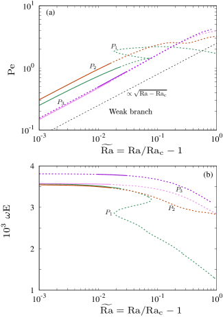
Figure 1: Bifurcation diagrams of rotating waves for the 3 sets of parameters: $P_{1}$ with $(\Pr,{\rm E})=(0.03,3\times 10^{-6})$, $P_{2}$ with $(\Pr,{\rm E})=(0.01,10^{-6})$, and $P_{3}$ with $(\Pr,{\rm E})=(0.003,3\times 10^{-7})$. For the set $P_{3}$ two different branches with $m_{0}=11$ (violet) and with $m_{0}=12$ (magenta) are shown. (a) Péclet number ${\rm Pe}$ versus ${\rm\widetilde{Ra}}={\rm Ra}/{\rm Ra_{c}}-1$. The dashed line indicates the $\sqrt{{\rm Ra}-{\rm Ra_{c}}}$ scaling predicted in Ecke et al. (1992). (b) Scaled rotating frequency $\omega{\rm E}$ versus ${\rm\widetilde{Ra}}$. Solid/dashed lines mark stable/unstable rotating waves.

We note that both, $\Pr$ and ${\rm E}$ roughly decrease by a factor of $3$ from $P_{1}$ to $P_{2}$, and from $P_{2}$ to $P_{3}$, so there is an increase of computational complexity from $P_{1}$ to $P_{3}$. As is clear from Table 1 the critical frequencies $\omega_{c}$ increase since the product $\omega_{c}{\rm E}$ remains very similar for all the cases. In addition, as the Prandtl and Ekman numbers are decreased the marginal stability curves for the onset of convection corresponding to a single azimuthal wave number approach each other (e. g. Net et al. (2008); Sánchez et al. (2016)) meaning that multitudes of radial and colatitudinal structures are unstable just after the onset.

The global quantity analyzed, in correspondence with Kaplan et al. (2017), is the Peclet number ${\rm Pe}=r_{o}U/\kappa$, which in terms of the dimensionless volume-averaged kinetic energy $K$ becomes ${\rm Pe}=(1-\eta)^{-1}\Pr~{}(2K)^{1/2}$. According to Kaplan et al. (2017) the Peclet number helps to identify if a solution belongs to the weak branch or not depending on whether ${\rm Pe}<10$ or not. This threshold separates flows dominated by diffusion (weak branch) to flows dominated by advection (strong branch). The frequencies of the RWs, $\omega{\rm E}$, or the volume-averaged kinetic energy $K_{m}$, computed by considering only the azimuthal wave number $m$ in the spherical harmonics expansion of the toroidal and poloidal potentials (Eqs. (6) and (7)), are also considered as global data. Regarding local data, the time series of the temperature perturbation, picked up at some points inside the fluid, and the time series of the real part of the poloidal amplitudes of Eq. (7) of different modes $(m,l)$ in the middle of the sphere, are considered.

III Rotating waves

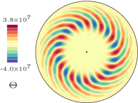
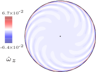
Figure 2: Rotating wave with $m_{0}=12$, in the case of the set $P_{3}$ (${\rm E}=3\times 10^{-7}$,${\rm Pr}=0.003$) and ${\rm Ra}=1.2634\times 10^{8}$ (${\rm\widetilde{Ra}}=7.9\times 10^{-3}$). Top row: Contour plots for the temperature perturbation $\Theta$ on an equatorial and meridional section. Bottom row: Contour plots for the vertical vorticity $\hat{\omega}_{z}$ on an equatorial section and for the azimuthal velocity $v_{\varphi}$ on a meridional section.

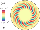
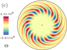
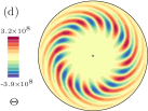
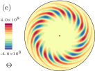
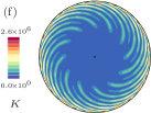
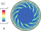
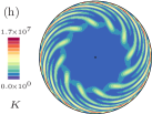
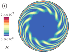
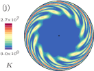
Figure 3: Rotating waves with $m_{0}=12$, in the case of the set $P_{3}$ (${\rm E}=3\times 10^{-7}$,${\rm Pr}=0.003$). Contour plots for the temperature perturbation $\Theta$ (top row) and for the kinetic energy density $K$ (bottom row) on an equatorial section. The Rayleigh numbers are ${\rm Ra}=1.3030\times 10^{8}$ (a,f), ${\rm Ra}=1.4511\times 10^{8}$ (b,g), ${\rm Ra}=1.5932\times 10^{8}$ (c,h), ${\rm Ra}=1.9650\times 10^{8}$ (d,i), and ${\rm Ra}=2.5067\times 10^{8}$ (e,j). This corresponds to ${\rm\widetilde{Ra}}=3.9\times 10^{-2}$, ${\rm\widetilde{Ra}}=1.6\times 10^{-1}$, ${\rm\widetilde{Ra}}=2.7\times 10^{-1}$, ${\rm\widetilde{Ra}}=5.7\times 10^{-1}$, and ${\rm\widetilde{Ra}}=10^{0}$.

By means of the continuation method described in § II.2 the bifurcation diagrams for RWs corresponding to the three sets, $P_{1}=(\Pr,{\rm E})=(0.03,3\times 10^{-6})$, $P_{2}=(\Pr,{\rm E})=(0.01,10^{-6})$, and $P_{3}=(\Pr,{\rm E})=(0.003,3\times 10^{-7})$, are obtained. For each set $P_{i}$ the azimuthal symmetry of the RWs correspond to that at the onset of convection given in Table 1. Concretely, $m_{0}=12$ for $P_{1}$, $m_{0}=11$ for $P_{2}$, and $m_{0}=12$ for $P_{3}$. Figure 1 displays the Peclet number ${\rm Pe}$ and the normalized rotation frequencies $\omega{\rm E}$ versus the parameter ${\rm\widetilde{Ra}}={\rm Ra}/{\rm Ra_{c}}-1$, which measures the departure from the onset. Stable (resp. unstable) RWs are denoted by solid (resp. dashed) lines.

Figure 1(a) is the same as Figure 1 of Kaplan et al. (2017) but note that in Kaplan et al. (2017) two additional sets, one at ${\rm E}=10^{-5}$ and the other at ${\rm E}=10^{-7}$, were displayed. To compare both figures one must take into account that slight deviations of the value of ${\rm Ra_{c}}$ imply important deviations in ${\rm Pe}$ for values of ${\rm\widetilde{Ra}}$ close to $10^{-2}$. For instance, if for the set $P_{2}$ we use ${\rm Ra_{c}}=5.475\times 10^{7}$, given in Kaplan et al. (2017), instead of our computed ${\rm Ra_{c}}=5.4949\times 10^{7}$, given in Table 1, we would obtain a value of ${\rm Pe}\approx 0.7$ (in agreement with Kaplan et al. (2017)) instead of ${\rm Pe}\approx 1$ marked in Figure 1(a). Note that for the set $P_{1}$ our results agree with those of Kaplan et al. (2017) since the critical Rayleigh numbers for this set have the same three first significant figures (see Table 1).

In contrast to Kaplan et al. (2017), we have found stable the branch of RWs with azimuthal symmetry $m_{0}=12$ (weak branch) bifurcating from the onset in the case of the set $P_{3}$. Certainly, these solutions can be found up to a critical value of the Rayleigh number marking the interval of stability of the branch. This interval is comparable to those of the weak branches bifurcating from the onset for the sets $P_{1}$ and $P_{2}$. Aside the branch of RWs with azimuthal symmetry $m_{0}=12$, we have computed a branch of RWs with azimuthal symmetry $m_{0}=11$. This branch is born unstable as it corresponds to the second preferred eigenfunction at the onset of convection but becomes stable very close to the onset. As it will be shown in the next sections, to assess the stability of these RWs, or to compute them using DNS, is a computationally challenging task.

Figure 1(a) evidences that all the branches follow the $\sqrt{{\rm Ra}-{\rm Ra_{c}}}$ scaling, since there’s a Hopf bifurcation breaking the axisymmetry of the basic state (Ecke et al. (1992)). This scaling is only valid close to the bifurcation point. Notice how the scaling is valid in a larger interval as we go from set $P_{1}$ to the set $P_{3}$ indicating that the validity of the scaling depends on the other parameters (${\rm Pr},{\rm E}$). In addition, very close to the onset the branches become more steep. This is only clear for the branch with $m_{0}=11$ corresponding to the set $P_{3}$ but also occurs for the other branches. Notice that for larger values of ${\rm\widetilde{Ra}}$ the Peclet number departs from the predicted scaling and in the case of the set $P_{1}$ two saddle-node bifurcations occur (the folds of the curve).

In figure 1(b) the dependence of the rotation frequencies on the Rayleigh number is analyzed by displaying $\omega{\rm E}$ versus ${\rm\widetilde{Ra}}$. We recall that the rotation frequency ($\omega$) of a RW with azimuthal symmetry $m_{0}$ is related to the critical frequency at the onset ($\omega_{c}$) by $\omega=-\omega_{c}/m_{0}$. This is clear when comparing the values of Fig. 1(b) at ${\rm\widetilde{Ra}}=10^{-3}$ with Table 1. Note that the frequencies $\omega$ remain nearly constant among the three different sets up to ${\rm\widetilde{Ra}}=2\times 10^{-2}$. From this point the frequency decreases significantly in the case of $P_{1}$. In addition, the frequencies of the branches bifurcating from the onset are almost equal for the three sets.

The flow and temperature patterns for a stable RW with azimuthal symmetry $m_{0}=12$ corresponding to the case $P_{3}$ at ${\rm Ra}=1.2634\times 10^{8}$ (${\rm\widetilde{Ra}}=7.9\times 10^{-3}$) are investigated in figure 2 and correspond to the patterns of a multicellular mode described in Net et al. (2008). The first row displays, from left to right, the contour plots of the temperature perturbation on the equatorial plane and on a meridional section. On the second row, the contour plots for the vertical vorticity $\hat{\omega}_{z}$ (normalized by the planetary vorticity $\hat{\omega}_{z}=\omega_{z}{\rm E}/2$) on an equatorial plane, and the contour plots for the azimuthal velocity $v_{\varphi}$ on a meridional section, are shown. The meridional sections cut relative maxima of the fields. All the fields shown in Fig. 2 were already shown in Figs. 2 and S2 of Kaplan et al. (2017), but for a solution corresponding to the case $P_{2}$ at ${\rm\widetilde{Ra}}=10^{-2}$ for which the flow patterns are very similar. The flow is strongly geostrophic displaying convective columns aligned with the rotation axis (see meridional sections). In addition, azimuthal velocity and vertical vorticity tend to be attached to the outer sphere and multicelullar spiral arms are clearly seen on the equatorial section for the temperature perturbation. Additional contour plots in the case of a tricelullar mode can be found in Figure 4 of Net et al. (2008).

The main effect of increasing the Rayleigh number is to slightly displace the hot fluid cells (i.e the maximum of temperature perturbation) towards the outer sphere, in the cylindrical radial direction (see the first row of Fig. 3), whereas the flow regions with maximum kinetic energy are progressively moved inwards, towards the inner sphere, although they still remain located close to the outer sphere (see the second row of Fig. 3). In addition, for ${\rm\widetilde{Ra}}>2.\times 10^{-1}$ (three rightmost plots), fluid motions start to develop near the middle of the shell developing a ring of vortices which displays a characteristic polygonal structure.

III.1 Stability of rotating waves

By means of the method described in Sec. II.2 the stability of RWs for each set of parameters is analyzed. We have found that for all the three sets the RWs become unstable due to Hopf bifurcations giving rise to modulated rotating waves (MRW). This scenario, which has been already described in Sánchez et al. (2013); Garcia et al. (2016) for thermal convection in rotating spherical shells, is typical in SO$(2)$ symmetric systems (Rand, 1982; Golubitsky et al., 2000; Crawford and Knobloch, 1991).

$N_{r}$	$L_{\text{max}}$	${\rm E}$	${\rm Pr}$	${\rm Ra}$	${\rm\widetilde{Ra}}$	$K$	$\omega$	$|\lambda|$	$m_{0}$
$60$	$156$	$3\times 10^{-6}$	$0.03$	$2.38589\times 10^{7}$	$2.0\times 10^{-2}$	$1.0981\times 10^{3}$	$1.1314\times 10^{3}$	$0.98915$	$12$
$70$	$192$	$3\times 10^{-6}$	$0.03$	$2.38589\times 10^{7}$	$2.0\times 10^{-2}$	$1.1036\times 10^{3}$	$1.1312\times 10^{3}$	$0.98923$	$12$
$80$	$154$	$10^{-6}$	$0.01$	$5.53968\times 10^{7}$	$8.2\times 10^{-3}$	$7.4015\times 10^{3}$	$3.4380\times 10^{3}$	$0.97097$	$11$
$100$	$198$	$10^{-6}$	$0.01$	$5.53968\times 10^{7}$	$8.2\times 10^{-3}$	$7.5082\times 10^{3}$	$3.4375\times 10^{3}$	$0.97033$	$11$
$100$	$192$	$3\times 10^{-7}$	$0.003$	$1.27467\times 10^{8}$	$1.7\times 10^{-2}$	$4.2477\times 10^{4}$	$1.1603\times 10^{4}$	$1.00214$	$12$
$120$	$192$	$3\times 10^{-7}$	$0.003$	$1.27467\times 10^{8}$	$1.7\times 10^{-2}$	$4.2723\times 10^{4}$	$1.1603\times 10^{4}$	$1.00218$	$12$

Table 2: Number of radial collocation points $N_{r}$, spherical harmonic truncation parameter $L_{\text{max}}$, Ekman ${\rm E}$, Prandtl ${\rm Pr}$, and Rayleigh ${\rm Ra}$ numbers, volume-averaged kinetic energy $K$, rotating frequency $\omega$, and modulus of the dominant Floquet multiplier $|\lambda|$, for rotating waves with azimuthal symmetry $m_{0}$. The value ${\rm\widetilde{Ra}}={\rm Ra}/{\rm Ra_{c}}-1$, where ${\rm Ra_{c}}$ is the critical Rayleigh number for the onset of convection, can be used to locate the rotating wave on the bifurcation diagram of Fig. 1(a).

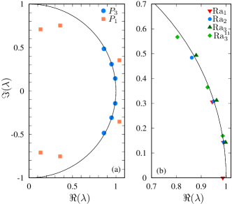
Figure 4: (a) Real and imaginary part of the leading Floquet multipliers $\lambda$ corresponding to the first unstable RWs with azimuthal symmetry $m_{0}=12$ for the set $P_{1}=(\Pr,{\rm E})=(0.03,3\times 10^{-6})$ (squares, orange online) and for the set $P_{3}=(\Pr,{\rm E})=(0.003,3\times 10^{-7})$ (circles, blue online). The Rayleigh numbers are ${\rm Ra}=2.43043\times 10^{7}$ (${\rm\widetilde{Ra}}=4\times 10^{-2}$) and ${\rm Ra}=1.27467\times 10^{8}$ (${\rm\widetilde{Ra}}=1.7\times 10^{-2}$), respectively. (b) Leading Floquet multipliers for the last stable (triangles down, red online) and first (circles, blue online) and second unstable (triangles up, dark-green online) RWs with azimuthal symmetry $m_{0}=12$ for the set $P_{3}$ at ${\rm Ra}_{1}=1.26344\times 10^{8}$, ${\rm Ra}_{2}=1.27467\times 10^{8}$, and ${\rm Ra}_{3}=1.3030\times 10^{8}$, respectively. The first unstable RW with azimuthal symmetry $m_{0}=11$ at ${\rm Ra}_{3}^{11}=1.3011\times 10^{8}$ is also shown (diamonds, green online). The conjugate Floquet multipliers are not shown in (b) and the solid line marks the unit circle.

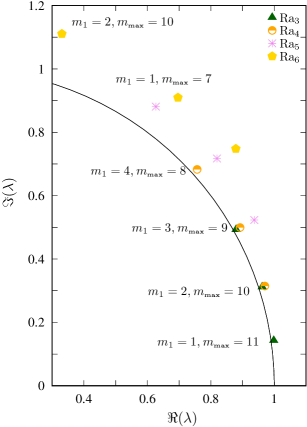
Figure 5: Leading Floquet multipliers for unstable RWs with azimuthal symmetry $m_{0}=12$ and the set $P_{3}$ (${\rm E}=3\times 10^{-7}$,${\rm Pr}=0.003$) at ${\rm Ra}_{3}=1.3030\times 10^{8}$ (triangles, dark-green online), at ${\rm Ra}_{4}=1.3228\times 10^{8}$ (circles, orange online), ${\rm Ra}_{5}=1.3919\times 10^{8}$ (asterisk, violet online), and ${\rm Ra}_{6}=1.4511\times 10^{8}$ (pentagon, yellow online). The labels indicate the azimuthal symmetry $m_{1}$ of the eigenfunction and its most energetic wave number $m_{\text{max}}$. The conjugate Floquet multipliers are not shown and the solid line marks the unit circle.

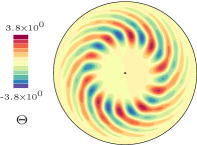
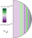
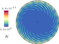
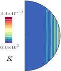
Figure 6: Leading eigenfunction of a RW with $m_{0}=11$, in the case of the set $P_{3}$ (${\rm E}=3\times 10^{-7}$,${\rm Pr}=0.003$), and ${\rm Ra}=1.3011\times 10^{8}$. Top row: Contour plots for the temperature perturbation $\Theta$ on an equatorial and meridional sections. Middle row: Contour plots for the vertical vorticity $\hat{\omega}_{z}$ on an equatorial section and for the azimuthal velocity $v_{\varphi}$ on a meridional section. Bottom row: Contour plots for the kinetic energy density $K$ on an equatorial and meridional sections. The azimuthal symmetry and most energetic wave number are $m_{1}=1$ and $m_{\text{max}}=10$, respectively.

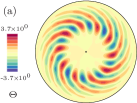
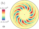
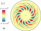
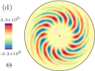
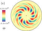
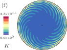
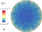
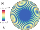
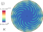
Figure 7: Leading eigenfunctions of rotating waves with $m_{0}=12$, in the case of the set $P_{3}$ (${\rm E}=3\times 10^{-7}$,${\rm Pr}=0.003$). Contour plots for the temperature perturbation $\Theta$ (top row) and for the kinetic energy density $K$ (bottom row) on an equatorial section. The Rayleigh numbers are ${\rm Ra}=1.3030\times 10^{8}$ (a,f), ${\rm Ra}=1.3228\times 10^{8}$ (b,g), ${\rm Ra}=1.3919\times 10^{8}$ (c,h), and ${\rm Ra}=1.4511\times 10^{8}$ (d,e,i,j). For the latter ${\rm Ra}$, (d,i) and (e,j) correspond to the 1st and 3rd leading eigenfunctions, respectively. Their respective azimuthal symmetry and most energetic wave number are $m_{1}=2$ and $m_{\text{max}}=10$, $m_{1}=3$ and $m_{\text{max}}=9$, $m_{1}=4$ and $m_{\text{max}}=8$, $m_{1}=2$ and $m_{\text{max}}=10$, and $m_{1}=1$ and $m_{\text{max}}=7$.

Specifically, the Hopf bifurcations occur at ${\rm Ra}=2.3903\times 10^{7}$ (${\rm\widetilde{Ra}}=2.2\times 10^{-2}$) for the set $P_{1}=(\Pr,{\rm E})=(0.03,3\times 10^{-6})$, at ${\rm Ra}=5.5823\times 10^{7}$ (${\rm\widetilde{Ra}}=1.6\times 10^{-2}$) for the set $P_{2}=(\Pr,{\rm E})=(0.01,10^{-6})$. For the set $P_{3}=(\Pr,{\rm E})=(0.003,3\times 10^{-7})$, RWs with $m_{0}=12$ become unstable at ${\rm Ra}=1.2731\times 10^{8}$ (${\rm\widetilde{Ra}}=1.6\times 10^{-2}$) and RWs with $m_{0}=11$ become unstable at ${\rm Ra}=1.2952\times 10^{8}$ (${\rm\widetilde{Ra}}=2.9\times 10^{-2}$). The values of ${\rm Ra}$ marking the bifurcation point have been obtained by linear interpolation between the last stable and the first unstable available RWs, which have the pairs $({\rm Ra}_{1},|\lambda_{1}|)$ and $({\rm Ra}_{2},|\lambda_{2}|)$, with $|\lambda_{1}|<1$ and $|\lambda_{2}|>1$, where $\lambda_{i}$ is the dominant Floquet multiplier. The values $({\rm Ra}_{i},|\lambda_{i}|)$, with $|\lambda_{i}|$ closest to unity, the volume-averaged kinetic energy $K$, and the rotation frequency $\omega$ of the RWs, are listed in Table 2 for the three sets of parameters and different resolutions to look for spatial discretization errors. We have found that the radial resolution is critical to correctly assess the stability of the waves. In the case of the set $P_{3}$ all the RWs have been found unstable if $N_{r}=80$ is employed.

Figure 4(a) displays the six leading Floquet multipliers for two unstable RWs corresponding to the sets $P_{1}$ (squares) and $P_{3}$ (circles) at ${\rm Ra}=2.43043\times 10^{7}$ (${\rm\widetilde{Ra}}=4\times 10^{-2}$) and at ${\rm Ra}=1.27467\times 10^{8}$ (${\rm\widetilde{Ra}}=1.7\times 10^{-2}$), respectively. For both cases any leading Floquet multiplier has its corresponding complex conjugate and for the set $P_{3}$ the leading Floquet multipliers are arranged near the unit circle. This is specially true for Rayleigh numbers close to the critical Rayleigh number determining the onset of unstable RWs, either for the branch of RWs with azimuthal symmetry $m_{0}=12$ or for the branch of RWs with azimuthal symmetry $m_{0}=11$, see Fig 4(b). In this figure, the solution at ${\rm Ra}_{3}=1.3030\times 10^{8}$ (${\rm\widetilde{Ra}}_{3}=3.9\times 10^{-2}$), corresponding to the branch with azimuthal symmetry $m_{0}=12$ and the set $P_{3}$, has the Floquet multipliers more clustered near the unit circle than the solution at a similar ${\rm\widetilde{Ra}}=4\times 10^{-2}$ (${\rm Ra}=2.43043\times 10^{7}$) for the set $P_{1}$ (shown in Fig. 4(a)). This means that $|\lambda|\equiv|\lambda({\rm\widetilde{Ra}})|$ is steeper in the case of the set $P_{1}$ and quite flat for the set $P_{3}$, at least near the onset of convection (${\rm\widetilde{Ra}}<0.1$). For this reason, the stability analysis for the RWs shown in Fig 4(b) is computationally challenging because of the convergence of the eigenvalue solver (Saad (1992)). Before starting the Arnoldi iteration procedure (Lehoucq et al. (1998)), more than 400 power method iterations have been performed to the initial guess to filter out the components associated to non-leading Floquet multipliers.

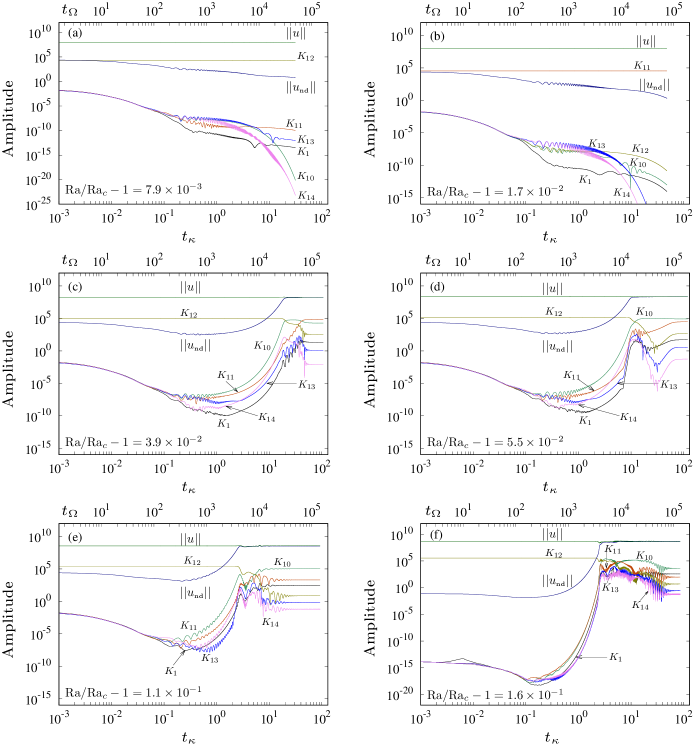
Figure 8: Time integration with initial conditions obtained by adding a random perturbation to the RWs for the set $P_{3}$ (${\rm E}=3\times 10^{-7}$,${\rm Pr}=0.003$). Norm of the amplitudes of the potential scalars and the temperature perturbation $||u||$, and the norm $||u_{\text{\tiny{nd}}}||$ for only $m\neq 12k,~{}k\in\mathbb{Z}$ (in (a,c,d,e,f)) and $m\neq 11k,~{}k\in\mathbb{Z}$ (in (b)), versus diffusion time (also rotation time on top horizontal axis). The volume averaged kinetic energies for each wave number $m=1,10,11,12,13,14$ are displayed as well. The Rayleigh numbers are (a) ${\rm Ra}=1.2634\times 10^{8}$, (b) ${\rm Ra}=1.2747\times 10^{8}$, (c) ${\rm Ra}=1.3030\times 10^{8}$, (d) ${\rm Ra}=1.3228\times 10^{8}$, (e) ${\rm Ra}=1.3919\times 10^{8}$, and (f) ${\rm Ra}=1.4511\times 10^{8}$.

Figure 5 displays the leading Floquet multipliers for several Rayleigh numbers up to ${\rm\widetilde{Ra}}=1.6\times 10^{-1}$ which are still located near the unit circle. This means that any perturbation applied to the RWs grows very slowly and gives rise to very long transients if DNS are employed. This will be illustrated later in Sec. IV. The study of the symmetry of the unstable eigenfunctions, when coupled with the symmetry of the RWs, allows to infer the spatial structure of MRWs which bifurcate from the branch of RWs (e.g. Sánchez et al. (2013); Garcia et al. (2016)). This is because close to the bifurcation point a MRW denoted by $u_{2}$ can be approximated by $u_{2}\approx u_{0}+\epsilon u_{1}$, where $u_{0}$ is the parent RW, $u_{1}$ is the leading Floquet mode, and $\epsilon$ is a small value. As the azimuthal symmetry of the RWs is $m_{0}=12$ only Floquet eigenfunctions with azimuthal symmetry $m_{1}\in\{1,2,3,4,6,12\}$ are possible ($m_{1}$ should be a factor of $m_{0}$) since the RWs and their eigenfunctions are coupled in the variational equations (e.g. Garcia et al. (2014)). In addition, at the bifurcation point, the azimuthal symmetry, $m_{2}$, of the MRW should be equal to $m_{1}$. The azimuthal symmetry $m_{1}$ and most energetic wave number $m_{\text{max}}$ of the corresponding eigenfunctions are labeled on each multiplier shown in Fig. 5. The figure shows that all the eigenvalues have azimuthal symmetry which is not $m_{1}=12$, meaning that the bifurcations broke the azimuthal symmetry giving rise to the excitation of low azimuthal wave numbers $m_{1}\in\{1,2,3,4\}$. Figure 5 also helps to visualize the increase of the real and imaginary parts of a given Floquet multiplier (described by the azimuthal symmetry and $m_{\text{max}}$) with the Rayleigh number.

The patterns of the temperature perturbation, axial vorticity, azimuthal velocity, and kinetic energy for the leading eigenfunction of a RW with azimuthal symmetry $m_{0}=11$ corresponding to the case $P_{3}$ at ${\rm Ra}=1.3011\times 10^{8}$ (${\rm\widetilde{Ra}}=3.8\times 10^{-2}$) are displayed in Fig. 6. The corresponding Floquet multiplier is shown in Fig. 4(b) (diamond at the bottom) and it is located just outside the unit circle, i.e. a Hopf bifurcation has occurred. The azimuthal symmetry of the eigenfunction is $m_{1}=1$ and the most energetic wave number is $m_{\text{max}}=10$ so the $m_{0}=11$ azimuthal symmetry of the parent RW is broken and MRWs with azimuthal symmetry $m_{1}=1$ develop. These MRWs are studied later on Sec. IV. As described for the RWs, the eigenfunction’s velocity field is aligned in the axial direction and attached to the outer sphere. There are 10 hot (cold) cells with larger magnitude for the temperature perturbation since $m_{\text{max}}=10$ but they have slightly different shapes due to the $m_{1}=1$ azimuthal symmetry. The latter symmetry is best displayed in the equatorial section of the kinetic energy contour plots where the spiraling arms form an oval structure in the interior of the sphere. The interior structures of this eigenfunction will be further studied in Sec. IV.1 and compared with the topology of nonlinear flows (MRWs) near the bifurcation point.

Figure 7 displays the topology of the eigenfunctions corresponding to some Floquet multipliers (shown in Fig. 5) with different azimuthal symmetries at different Rayleigh numbers. The temperature and velocity patterns are multicellular and look very similar to those analyzed in Fig. 6. By increasing ${\rm Ra}$ the main difference is that the temperature cells as well as kinetic energy vortices tend to move to the interior of the fluid as was the case for RWs (see Fig. 3). Similarly to the case of the leading eigenfunction at ${\rm Ra}=1.3011\times 10^{8}$ the spiralling arms for the leading eigenfunction at ${\rm Ra}=1.3030\times 10^{8}$ (leftmost plot of the kinetic energy density, Figure 7) form a regular pattern, a square in this case, in the interior of the sphere.

IV Time evolutions for ${\rm E}=3\times 10^{-7}$ and ${\rm Pr}=0.003$

The aim of this section is to investigate oscillatory flows for the set $P_{3}$ obtained for ${\rm Ra}$ larger than that required for the stability of RWs. The analysis is conducted by performing DNS with selected initial conditions, at different ${\rm Ra}$, along the branch of RWs already studied in Sec. III. For each initial condition a random perturbation (of order $10^{-6}$) to all spherical harmonic amplitudes is added and the system is integrated around $100$ diffusion time units, which is more than one order of magnitude larger than the typical final times of the DNS presented in Kaplan et al. (2017). This is particularly challenging since the dimension of the system is of order $10^{7}$ ($N_{r}=100$ and $L_{\text{max}}=192$ are used) and a time step of $1.7\times 10^{-5}$ diffusion time units is employed.

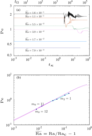
Figure 9: (a) Peclet number versus diffusion time (also rotation time on top horizontal axis), in the case of the set $P_{3}$ (${\rm E}=3\times 10^{-7}$,${\rm Pr}=0.003$) for the same solutions as shown in Fig. 8. The Rayleigh numbers, increasing from bottom to top, are ${\rm Ra}=1.2634\times 10^{8}$, ${\rm Ra}=1.2747\times 10^{8}$, ${\rm Ra}=1.3030\times 10^{8}$, ${\rm Ra}=1.3228\times 10^{8}$, ${\rm Ra}=1.3919\times 10^{8}$, and ${\rm Ra}=1.4511\times 10^{8}$. (b) Bifurcation diagrams of the time averaged Peclet number corresponding to the branches of RWs with azimuthal symmetry $m_{0}=12$ and $m_{0}=11$ and of MRWs with azimuthal symmetry $m_{2}=1$. The points correspond to the curves shown in (a).

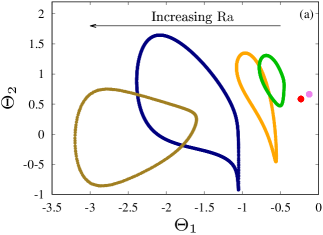
Figure 10: (a) Poincaré section defined by $0=\Theta(r,\varphi,\theta)$ with $(r,\varphi,\theta)=(0.51,0,5\pi/8)$. The temperatures $\Theta_{1}=\Theta(0.16,0,5\pi/8)$ and $\Theta_{2}=\Theta(0.86,0,5\pi/8)$ are displayed on the horizontal and vertical axis, respectively. We recall that $\eta=0.01$ implies $r_{i}=0.0101$ and $r_{o}=1.0101$ and that solutions belong to the set $P_{3}$ (${\rm E}=3\times 10^{-7}$,${\rm Pr}=0.003$). The Rayleigh numbers of each section increase from right to left in the figures (see the arrow). They are ${\rm Ra}=1.2634\times 10^{8}$, ${\rm Ra}=1.2747\times 10^{8}$, ${\rm Ra}=1.3030\times 10^{8}$, ${\rm Ra}=1.3228\times 10^{8}$, ${\rm Ra}=1.3919\times 10^{8}$, and ${\rm Ra}=1.4511\times 10^{8}$, corresponding to panels (a),(b),(c),(d),(e) and (f), respectively, of Fig. 8.

Figure 11: (a) Temperature $\Theta_{3}=\Theta(r,\varphi,\theta)$, with $(r,\varphi,\theta)=(0.51,0,5\pi/8)$, versus diffusion time. (b) Same as (a) but for the temperature $\Theta_{1}=\Theta(0.16,0,5\pi/8)$. The Rayleigh number is ${\rm Ra}=1.4511\times 10^{8}$ corresponding to panel (f) of Fig. 8. The solution belongs to the set $P_{3}$ (${\rm E}=3\times 10^{-7}$,${\rm Pr}=0.003$). The time averages of the kinetic energy spectra of Fig. 12(a) and Fig. 12(b) are taken over the time intervals $I_{1}$ and $I_{2}$, respectively. (c) and (e) correspond to details of (a) in the intervals $I_{1}$ and $I_{2}$, respectively. (d) and (f) correspond to details of (b) in the intervals $I_{1}$ and $I_{2}$, respectively.

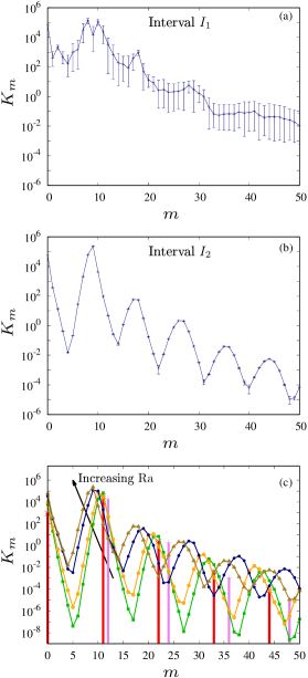
Figure 12: Time and volume averaged kinetic energy spectra $K_{m}$ versus the azimuthal wave number $m$. In (a) and (b) the Rayleigh number is ${\rm Ra}=1.4511\times 10^{8}$ and the time average is taken over the interval $I_{1}$ and $I_{2}$, respectively, which are shown in Fig. 11. In (c) several Rayleigh numbers are shown which increase from right to left in the figure (see the arrow). They are ${\rm Ra}=1.2634\times 10^{8}$, ${\rm Ra}=1.2747\times 10^{8}$, ${\rm Ra}=1.3030\times 10^{8}$, ${\rm Ra}=1.3228\times 10^{8}$, ${\rm Ra}=1.3919\times 10^{8}$, and ${\rm Ra}=1.4511\times 10^{8}$, corresponding to panels (a),(b),(c),(d),(e) and (f), respectively, of Fig. 8. All these solutions belong to the set $P_{3}$ (${\rm E}=3\times 10^{-7}$,${\rm Pr}=0.003$). For each $m$, the maximum and minimum values of $K_{m}$ over the time interval are shown with error bars. The ime average, maximum and minimum values are taken over the last 5 diffusion time units of each time series.

Figure 8 illustrates the procedure by displaying the volume-averaged kinetic energy $K_{m}$ for each azimuthal wave number $m\in\{1,10,11,12,13,14\}$ versus time in diffusion units (also in rotation units) for the DNS corresponding to different ${\rm Ra}$. In each panel the norm $||u||$, of the vector containing the amplitudes of the scalar potentials and the temperature perturbation, and the norm $||u||_{\text{nd}}$ -when only the azimuthal wave numbers which are not multiples of $m_{0}=12$ (or $m_{0}=11$ for panel (b)) are considered- are plotted as well. The initial condition corresponds to a stable RW with azimuthal symmetry $m_{0}=12$ in Fig. 8(a), and to a stable RW with azimuthal symmetry $m_{0}=11$ in Fig. 8(b), and thus the added random perturbation (affecting all the spherical harmonics of the RWs) is damped but on a very large time scale, see the curve of $||u||_{\text{nd}}$ containing the norm of vector containing the spherical harmonic amplitudes of the azimuthal wave numbers which are not multiple of $m_{0}$. In agreement with the results presented in Sec. III.1 the azimuthal wave numbers for which $K_{m}$ decreases more slowly correspond to the azimuthal symmetry $m_{1}$ and the most energetic wave number $m_{\text{max}}$ of the leading eigenfunction, because the associated eigenvalues are very close to the unit circle (see Fig. 4(b)). The slowly damped modes are $m=1$ and $m=11$ for the RW with azimuthal symmetry $m_{0}=12$ (Fig. 8(a)) and $m=1$ and $m=10$ (Fig. 8(b)) for the RW with azimuthal symmetry $m_{0}=11$. Notice that in Fig. 8(a) the mode $m=13$ is slowly damped as well because of the coupling of the azimuthal symmetry of the RW $m_{0}=12$ and the azimuthal symmetry of the eigenfunction $m_{1}=1$. The same occurs in Fig. 8(b) for the mode $m=12$.

For the same arguments as described above (i.e. the eigenvalues of the eigenfunctions are clustered around the unit circle) the perturbations added to unstable RWs grow very slowly and the stable attractor is reached on a very large time scale. This is displayed in Fig. 8(c,d,e,f) where at least 30 diffusion times (or $5\times 10^{4}$ planetary rotations) are needed to saturate the flow. In all the cases after a sharp increase of the unstable modes (after around 2-10 diffusion times) a strongly oscillatory transient lasts more than 30 diffusion times. The final attractor is a MRW, i.e. a quasiperiodic flow with two incommensurable frequencies, which has a certain spatio-temporal symmetry. Notice that for MRW the value of $||u||_{\text{nd}}$ is almost equal to $||u||$ since the spherical harmonics amplitudes corresponding to the azimuthal wave numbers $m=12k,~{}k\in\mathbb{Z}$ are significantly smaller when compared with other azimuthal wave numbers (for instance $m=10$). The systematic computation of MRW has been performed in Garcia et al. (2016) for the same problem as described here but for spherical shells. These types of oscillatory flows are still in the weak branch regime since their Peclet numbers are of order one. This is illustrated in Fig. 9(a) where the time series of the Peclet number ${\rm Pe}$ are displayed for the same solutions as analyzed in Fig. 8. Figure 9(b) corresponds to the bifurcation diagrams of the time-averaged ${\rm Pe}$ for these MRWs including also the branches of RWs already displayed in Fig. 1.

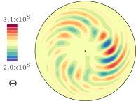
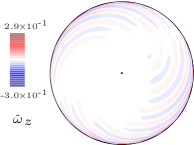
Figure 13: Solution bifurcating from rotating waves with $m_{0}=12$, in the case of the set $P_{3}$ (${\rm E}=3\times 10^{-7}$,${\rm Pr}=0.003$) at ${\rm Ra}=1.4511\times 10^{8}$. The snapshot is taken in the transient phase, at the end of the time interval $I_{1}$ shown in Fig. 11(a). Top row: Contour plots for the temperature perturbation $\Theta$ on an equatorial and meridional section. Bottom row: Contour plots for the vertical vorticity $\hat{\omega}_{z}$ on an equatorial section and for the azimuthal velocity $v_{\varphi}$ on a meridional section.

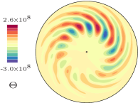
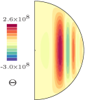
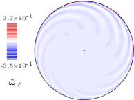
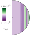
Figure 14: As Fig. 13 but with the snapshot taken in the saturated phase, at the end of the time interval $I_{2}$ shown in Fig. 11(a).

To demonstrate the quasiperiodic nature of MRWs, Poincaré sections, extracted from the time series of temperature perturbation, are displayed in Fig. 10 for the same solutions as analyzed in Fig. 8 (points in Fig. 9(b)). The Poincaré section of a RW (periodic flow) is a point, whereas it corresponds to a closed curve in the case of MRWs (quasiperiodic flow). Increasing the Rayleigh number up to ${\rm Ra}=1.3919\times 10^{8}$ results in larger oscillations of the temperature perturbation since the curves enclose a larger area. Notice that for ${\rm Ra}=1.4511\times 10^{8}$ the curve spreads over a smaller interval in the vertical axis than in the case of ${\rm Ra}=1.3919\times 10^{8}$ so the oscillations of temperature close to the outer boundary become smaller.

To further investigate the nature of the temperature fluctuations, the time series of $\Theta$ are displayed in Fig. 11(a,b) at two different points close to the equatorial plane (see figure caption), one in the middle of the sphere (panel (a)) and the other close to the inner boundary (panel (b)). The time series are for the MRW at ${\rm Ra}=1.4511\times 10^{8}$ corresponding to panel (f) of Fig. 8. In Fig. 11(a,b) the long initial transients (around 50 diffusion times) required to saturate this solution (see discussion of Fig. 8) are clearly visible. Figure 11(c,d) displays a detail of Fig. 11(a) (i.e. $\Theta$ in the middle of the sphere) in two different time intervals, one during the transient phase (interval $I_{1}$), and the other during the saturated phase (interval $I_{2}$) of the solution. Figure 11(e,f) is as Fig. 11(c,d) but displays the details of Fig. 11(b) (i.e. $\Theta$ close to the center of the sphere). The comparison between the different panels summarizes several facts. First, the oscillations have different main time scales depending on whether $\Theta$ is measured in the middle of the shell (small and large scales, clearly quasiperiodic) or close to the center of the sphere (mainly large scales and periodic). Second, the long transients (interval $I_{1}$) exhibit intermittent-like structures. Finally, for the long transients an intermediate time scale is additionally present for $\Theta$ picked up close to the center of the sphere.

The mode structure of the long initial transients and the saturated MRW at ${\rm Ra}=1.4511\times 10^{8}$ is significantly different. This is demonstrated in Fig. 12 displaying the time averaged kinetic energy spectra versus the azimuthal wave number $m$ over the interval $I_{1}$ (panel (a)) and over the time interval $I_{2}$ (panel (b)). The figure also displays (with error bars) the amplitude of the kinetic energy oscillations. The transients are characterized by strong time oscillations of all the modes. In addition the flow is bimodal, in the sense that the azimuthal wave numbers $m=8$ and $m=10$ have maximum energy. Also, low wave numbers $m<6$ have a similar and noticeable (larger than $10^{2}$) magnitude. In contrast, the kinetic energy spectra of the saturated MRW have a single maximum (at $m=9$) and the time dependence of $K_{m}$ is only noticeable for the modes at the relative minima of the spectrum. In addition, only the low wave number $m=1$ has magnitude larger than $10^{2}$. The other MRWs analyzed in the previous figures have similar kinetic energy spectra as shown in Fig. 12(c). In this figure RWs have nonzero kinetic energy only in the wave numbers of the form $km_{0},~{}k\in\mathbb{Z}$ ($m_{0}$ is the azimuthal symmetry of the RW) whereas MRWs, all of them with azimuthal symmetry $m_{2}=1$, have nonzero kinetic energy in all the modes. As the Rayleigh number is increased $m_{\text{max}}$ decreases (from $m=12$ at the smallest ${\rm Ra}$ down to $m=9$ at the largest ${\rm Ra}$). Moreover, the relative difference between dominant modes (relative maxima) and non-dominant modes (relative minima) decreases. Notice that for the low wave numbers (specially $m=5$) the kinetic energy $K_{m}$ sharply increases with ${\rm Ra}$. Scalloped spectra like those of Fig. 12(b,c), already studied for the case of the spherical Couette flow in Marcus and Tuckerman (1987), are a consequence of a periodic spatial structure modulated by an envelope as is shown in the following paragraph.

The flow and temperature spatial structures during the transient as well as the saturated phase for the DNS at ${\rm Ra}=1.4511\times 10^{8}$ can be visualized in Fig. 13 and Fig. 14, respectively. In both cases the flow is strongly geostrophic; the temperature perturbation exhibit multicellular patterns, and the maximum azimuthal velocity is located close to the outer sphere as described for the RWs in Sec. III. In contrast to RWs, the shapshots presented in Fig. 13 and Fig. 14 have a clear asymmetry (a modulation by an envelope as described in Marcus and Tuckerman (1987)) between temperature cells because of the excitation of low wave numbers (see Fig. 12) predicted by the stability analysis conducted in Sec. III.1. The main difference between the contour plots of the transient flow and the saturated phase (Fig. 13 and Fig. 14, respectively) is that, for the former, the azimuthal asymmetry of the $m=10$ structure is more irregular (i. e. modulated by several low wave numbers) whereas for the latter the azimuthal modulation is mainly due to $m=1$. A further description of the flow and temperature patterns for a MRW, in terms of its different mode components, will be provided in the next section, Sec. IV.1.

IV.1 Triadic resonances

In this section we add further evidence to the recent study of Garcia et al. (2021a) in which triadic resonances occurring in spherical systems have been interpreted in terms of MRWs. Triadic resonances in the spherical Couette problem have been comprehensively studied in Barik et al. (2018) and are characterized by the existence of azimuthal wave numbers $m_{i}$, $m_{j}$ and $m_{k}$ with main time dependencies provided by the frequencies $\omega_{i}$, $\omega_{j}$, and $\omega_{k}$, respectively, for which the relations $m_{i}=m_{j}\pm m_{k}$ and $\omega_{i}=\omega_{j}\pm\omega_{k}$ hold. Triadic resonances as described in Barik et al. (2018) have been also analyzed in Lin (2021) for the same problem as studied here but for ${\rm E}\geq 10^{-6}$. As will be shown in the following, multiple resonances between several modes can be identified from the DNS of the MRWs previously studied. The resonant modes are excited by the Hopf bifurcations giving rise to MRWs (see Garcia et al. (2021a)).

Following the same procedure as in Garcia et al. (2021a) the time series of the real part of the poloidal amplitudes of Eq. (7), $\Re{\Phi^{m}_{l}(r_{o}/2)}$ for several $m\in\{1,...,20\}$ and $l\in\{1,...,40\}$, are considered to investigate the time scales of the flow and triadic resonances among the different modes $(m,l)$. We have considered two different MRWs at ${\rm Ra}=1.3030\times 10^{8}$ and at ${\rm Ra}=1.3919\times 10^{8}$. The 1st MRW is very close to the bifurcation point from the branch of RWs with $m_{0}=11$ (see the left point on the $m_{2}=1$ branch of Fig. 9(b)) whereas the 2nd MRW is far away (2nd rightmost point on the $m_{2}=1$ branch of Fig. 9(b))).

An accurate frequency analysis, based on Laskar’s algorithm Laskar (1993), has been applied to each of the time series to determine the fundamental frequencies. We note that for a time series of a large scale magnetohydrodynamic periodic flow Laskar’s algorithm detects the main frequency up to a relative error of order $10^{-5}$ (see discussion in Sec. 3.1 of Garcia et al. (2021b)). Because the flow is equatorially symmetric (see meridional sections of Fig. 14) we have considered the modes with $(m,l)=(m,m)$ which are equatorially symmetric for the poloidal potential. Other equatorially symmetric modes, such as $(m,m+2)$, are not considered since their time dependence is analogous to that of the mode $(m,m)$ (see Garcia et al. (2021a)). The frequencies, normalized by the global rotation of the sphere $\Omega$, are $\omega_{m}/\Omega=2\pi f_{m}{\rm E}$, where $f_{m}$ is the main peak in the dimensionless frequency spectrum. They are plotted in Fig. 15(a) for each mode $(m,l)=(m,m)$ and $1\leq m\leq 20$. Figure 15(b) displays the frequencies $\omega^{2}_{m}/\Omega$ obtained from the second largest peak in the frequency spectrum (so $\omega^{2}_{m}$ is not the square of $\omega_{m}$).

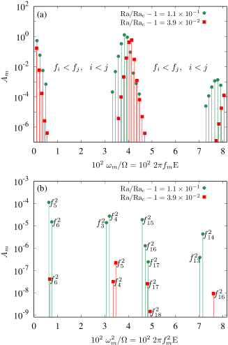
Figure 15: Frequency analysis for two solutions at ${\rm Ra}=1.3030\times 10^{8}$ (squares) and at ${\rm Ra}=1.3919\times 10^{8}$ (circles), in the case of the set $P_{3}$ (${\rm E}=3\times 10^{-7}$,${\rm Pr}=0.003$). (a) Leading frequencies, $f_{m}$, and amplitudes, $A_{m}$, of the time series of poloidal component, $\Re{\Phi^{m}_{m}(r_{d})}$, of the different modes $(m,m)$, $1\leq m\leq 20$. (b) as in (a) but for the 2nd leading frequencies $f^{2}_{m}$.

As in Garcia et al. (2021a), the leading frequencies of the modes $(i,i)$ and $(j,j)$ verify $\omega_{i}<\omega_{j}$ if $i<j$, so the frequencies are ordered following the azimuthal wave number ordering. A characteristic feature seen in Fig. 15(a) is that there exists a particular distribution of the frequencies, in the sense that there are separated blocks of clustered frequencies. The three blocks of Fig. 15(a) are $\omega_{m}/\Omega<0.006$, $0.032<\omega_{m}/\Omega<0.048$, and $\omega_{m}/\Omega>0.072$, which are associated to slow, moderate, and fast modes that correspond to small, moderate and large azimuthal wave numbers. For the MRW at ${\rm Ra}=1.3030\times 10^{8}$ these are $m\leq 5$, $6\leq m\leq 16$, and $m\geq 17$, respectively. In contrast, the secondary frequencies shown in Fig. 15(b) are not ordered with respect to the wave number but still retain the block structure. As it will be shown later in this section these secondary frequencies provide additional resonances among the modes. Notice that only the modes $m\in\{3,4,5,6,13,14,15,16,17,18\}$ have a secondary peak in the frequency spectrum and thus are quasiperiodic. These modes are those located contiguously at the boundaries of the block regions, see for instance the modes $m=4,5,6$ in the case of the MRW at ${\rm Ra}=1.3030\times 10^{8}$ in Fig. 15(a). The other modes $m\in\{1,2,7,8,9,10,11,19,20\}$ are purely periodic and lie in the interior of the block regions.

Figure 15 can be easily compared with Table I of Lin (2021). In that study, for ${\rm E}=10^{-6}$ and ${\rm Pr}=0.001$, the resonance conditions involving the azimuthal wave numbers $m_{i}=4$, $m_{j}=1$ and $m_{k}=3$, were found. The associated frequencies were $\omega_{i}/\Omega=0.25$, $\omega_{j}/\Omega=0.16$, and $\omega_{k}/\Omega=0.09$ which are roughly one order of magnitude larger than those presented in Fig. 15 for the low azimuthal wave numbers $m<5$. This is not surprising since our Ekman number (${\rm E}=3\times 10^{-7}$) is smaller.

Table 3: Relations between the main frequencies $f_{m}$ of the different modes $(m,l)=(m,m)$ for the 2T MRW with $m_{2}=1$ azimuthal symmetry at ${\rm Ra}=1.3030\times 10^{8}$. For the modes with $m\in\{4,5,6\}$ the spectrum has two peaks $f_{m}$ and $f^{2}_{m}$. These relations are satisfied up to $(f_{m_{i}}-f_{m_{j}}-f_{m_{k}})/f_{m_{i}}<\epsilon_{f}$ with $\epsilon_{f}=10^{-4}$.

$m=3$	$m=4$	$m=5$	$m=6$	$m=7$	$m=8$
$f_{3}=f_{1}+f_{2}$	$f_{4}=f_{1}+f_{3}$	$f_{5}=f_{1}+f_{4}$	$f_{6}=f_{1}+f^{2}_{5}$	$f_{7}=f_{1}+f_{6}$	$f_{8}=f_{1}+f_{7}$
	$\hskip 11.38109pt=2f_{2}$	$\hskip 11.38109pt=f_{2}+f_{3}$	$\hskip 11.38109pt=f_{2}+f^{2}_{4}$	$\hskip 11.38109pt=f_{2}+f^{2}_{5}$	$\hskip 11.38109pt=f_{2}+f_{6}$
		$f^{2}_{5}=f_{1}+f^{2}_{4}$	$f^{2}_{6}=f_{1}+f_{5}$	$\hskip 11.38109pt=f_{3}+f^{2}_{4}$	$\hskip 11.38109pt=f_{3}+f^{2}_{5}$
			$\hskip 11.38109pt=f_{2}+f_{4}$
			$\hskip 11.38109pt=2f_{3}$
$m=9$	$m=10$	$m=11$	$m=12$	$m=13$	$m=14$
$f_{9}=f_{1}+f_{8}$	$f_{10}=f_{1}+f_{9}$	$f_{11}=f_{1}+f_{10}$	$f_{12}=f_{1}+f_{11}$	$f_{13}=f_{1}+f_{12}$	$f_{14}=f_{1}+f_{13}$
$\hskip 11.38109pt=f_{2}+f_{7}$	$\hskip 14.22636pt=f_{2}+f_{8}$	$\hskip 14.22636pt=f_{2}+f_{9}$	$\hskip 14.22636pt=f_{2}+f_{10}$	$\hskip 14.22636pt=f_{2}+f_{11}$	$\hskip 14.22636pt=f_{2}+f_{12}$
$\hskip 11.38109pt=f_{3}+f_{6}$	$\hskip 14.22636pt=f_{3}+f_{7}$	$\hskip 14.22636pt=f_{3}+f_{8}$	$\hskip 14.22636pt=f_{3}+f_{9}$	$\hskip 14.22636pt=f_{3}+f_{10}$	$\hskip 14.22636pt=f_{3}+f_{11}$
$\hskip 11.38109pt=f_{4}+f^{2}_{5}$	$\hskip 14.22636pt=f_{4}+f_{6}$	$\hskip 14.22636pt=f_{4}+f_{7}$	$\hskip 14.22636pt=f_{4}+f_{8}$	$\hskip 14.22636pt=f_{4}+f_{9}$	$\hskip 14.22636pt=f_{4}+f_{10}$
$\hskip 11.38109pt=f^{2}_{4}+f_{5}$	$\hskip 14.22636pt=f^{2}_{4}+f^{2}_{6}$	$\hskip 14.22636pt=f_{5}+f_{6}$	$\hskip 14.22636pt=f_{5}+f_{7}$	$\hskip 14.22636pt=f_{5}+f_{8}$	$\hskip 14.22636pt=f_{5}+f_{9}$
		$\hskip 14.22636pt=f^{2}_{5}+f^{2}_{6}$		$\hskip 14.22636pt=f^{2}_{6}+f_{7}$	$\hskip 14.22636pt=f^{2}_{6}+f_{8}$

Table 4: Relations between the main frequencies $f_{m}$ of the different modes $(m,l)=(m,m)$ for the 2T MRW with $m_{2}=1$ azimuthal symmetry at ${\rm Ra}=1.3919\times 10^{8}$. For the modes with $m\in\{3,4,5,6,13,14\}$ the spectrum has two peaks $f_{m}$ and $f^{2}_{m}$. These relations are satisfied up to $(f_{m_{i}}-f_{m_{j}}-f_{m_{k}})/f_{m_{i}}<\epsilon_{f}$ with $\epsilon_{f}=10^{-4}$.

$m=3$	$m=4$	$m=5$	$m=6$	$m=7$	$m=8$
$f_{3}=f_{1}+f_{2}$	$f_{4}=f_{1}+f_{3}$	$f_{5}=f_{1}+f^{2}_{4}$	$f_{6}=f_{1}+f_{5}$	$f_{7}=f_{1}+f_{6}$	$f_{8}=f_{1}+f_{7}$
	$\hskip 11.38109pt=2f_{2}$	$\hskip 11.38109pt=f_{2}+f^{2}_{3}$	$\hskip 11.38109pt=f_{2}+f^{2}_{4}$	$\hskip 11.38109pt=f_{2}+f_{5}$	$\hskip 11.38109pt=f_{2}+f_{6}$
	$f^{2}_{4}=f_{1}+f^{2}_{3}$	$f^{2}_{5}=f_{1}+f_{4}$	$f^{2}_{6}=f_{1}+f^{2}_{5}$	$\hskip 11.38109pt=f_{3}+f^{2}_{4}$	$\hskip 11.38109pt=f_{3}+f_{5}$
		$\hskip 11.38109pt=f_{2}+f_{3}$	$\hskip 11.38109pt=f_{2}+f_{4}$	$\hskip 11.38109pt=f^{2}_{3}+f_{4}$	$\hskip 11.38109pt=f^{2}_{3}+f^{2}_{5}$
			$\hskip 11.38109pt=2f_{3}$
$m=9$	$m=10$	$m=11$	$m=12$	$m=13$	$m=14$
$f_{9}=f_{1}+f_{8}$	$f_{10}=f_{1}+f_{9}$	$f_{11}=f_{1}+f_{10}$	$f_{12}=f_{1}+f_{11}$	$f_{13}=f_{1}+f_{12}$	$f_{14}=f_{1}+f_{13}$
$\hskip 11.38109pt=f_{2}+f_{7}$	$\hskip 14.22636pt=f_{2}+f_{8}$	$\hskip 14.22636pt=f_{2}+f_{9}$	$\hskip 14.22636pt=f_{2}+f_{10}$	$\hskip 14.22636pt=f_{2}+f_{11}$	$\hskip 14.22636pt=f_{2}+f_{12}$
$\hskip 11.38109pt=f_{3}+f_{6}$	$\hskip 14.22636pt=f_{3}+f_{7}$	$\hskip 14.22636pt=f_{3}+f_{8}$	$\hskip 14.22636pt=f_{3}+f_{9}$	$\hskip 14.22636pt=f_{3}+f_{10}$	$\hskip 14.22636pt=f_{3}+f_{11}$
$\hskip 11.38109pt=f^{2}_{3}+f^{2}_{6}$	$\hskip 14.22636pt=f_{4}+f_{6}$	$\hskip 14.22636pt=f_{4}+f_{7}$	$\hskip 14.22636pt=f_{4}+f_{8}$	$\hskip 14.22636pt=f_{4}+f_{9}$	$\hskip 14.22636pt=f_{4}+f_{10}$
$\hskip 11.38109pt=f_{4}+f_{5}$	$\hskip 14.22636pt=f^{2}_{4}+f^{2}_{6}$	$\hskip 14.22636pt=f^{2}_{5}+f_{6}$	$\hskip 14.22636pt=f^{2}_{5}+f_{7}$	$\hskip 14.22636pt=f^{2}_{5}+f_{8}$	$\hskip 14.22636pt=f^{2}_{5}+f_{9}$
$\hskip 11.38109pt=f^{2}_{4}+f^{2}_{5}$		$\hskip 14.22636pt=f_{5}+f^{2}_{6}$		$\hskip 14.22636pt=f^{2}_{6}+f_{7}$	$\hskip 14.22636pt=f^{2}_{6}+f_{8}$
				$f^{2}_{13}=f^{2}_{3}+f_{10}$	$f^{2}_{14}=f^{2}_{3}+f_{11}$
				$\hskip 14.22636pt=f^{2}_{4}+f_{9}$	$\hskip 14.22636pt=f^{2}_{4}+f_{10}$
				$\hskip 14.22636pt=f_{5}+f_{8}$	$\hskip 14.22636pt=f_{5}+f_{9}$
				$\hskip 14.22636pt=f_{6}+f_{7}$	$\hskip 14.22636pt=f_{6}+f_{8}$
					$\hskip 14.22636pt=2f_{7}$

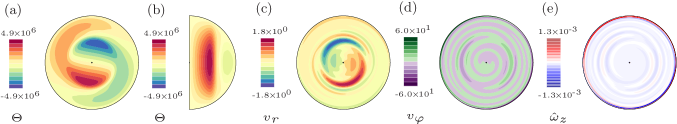
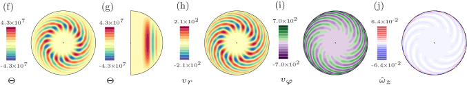
Figure 16: Modulated rotating wave with azimuthal symmetry $m_{2}=1$ in the case of the set $P_{3}$ (${\rm E}=3\times 10^{-7}$,${\rm Pr}=0.003$) at ${\rm Ra}=1.3030\times 10^{8}$. The contour plots of the temperature perturbation $\Theta$ on an equatorial (a,f,k) and a meridional (b,g,l) section, and of the radial velocity $v_{r}$ (c,h,m), azimuthal velocity $v_{\varphi}$ (d,i,n), and vertical vorticity $\hat{w}_{z}$ (e,j,o), normalized by the planetary vorticity $\hat{w}_{z}=w_{z}{\rm E}/2$, on equatorial sections, are displayed from left to right in each row. From top to bottom only the $m=1$ (a-e), $m=10$ (f-j) and $m=21$ (k-o), respectively, azimuthal wave numbers, rather than all $m$’s, are considered for the contour plots.

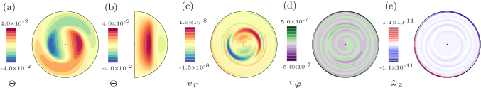
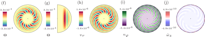
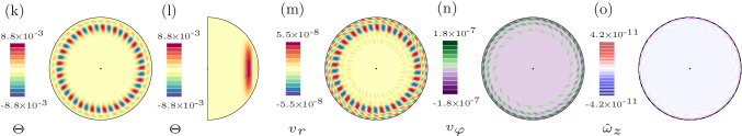
Figure 17: Leading eigenfunction, with azimuthal symmetry $m_{1}=1$, of a rotating wave with $m_{0}=11$, in the case of the set $P_{3}$ (${\rm E}=3\times 10^{-7}$,${\rm Pr}=0.003$) at ${\rm Ra}=1.3011\times 10^{8}$. The contour plots of the temperature perturbation $\Theta$ on an equatorial (a,f,k) and a meridional (b,g,l) section, and of the radial velocity $v_{r}$ (c,h,m), azimuthal velocity $v_{\varphi}$ (d,i,n), and vertical vorticity $\hat{w}_{z}$ (e,j,o), normalized by the planetary vorticity $\hat{w}_{z}=w_{z}{\rm E}/2$, on equatorial sections, are displayed from left to right in each row. From top to bottom only the $m=1$ (a-e), $m=10$ (f-j) and $m=21$ (k-o), respectively, azimuthal wave numbers, rather than all $m$’s, are considered for the contour plots.

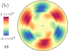
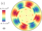
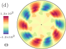
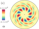
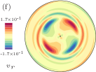
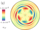
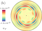
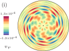
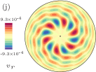
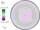
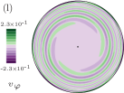
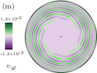
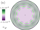
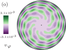
Figure 18: Modulated rotating wave with azimuthal symmetry $m_{2}=1$ at in the case of the set $P_{3}$ (${\rm E}=3\times 10^{-7}$,${\rm Pr}=0.003$) at ${\rm Ra}=1.3030\times 10^{8}$. The contour plots of the temperature perturbation $\Theta$ (a-e), of the radial velocity $v_{r}$ (f-j), and of the azimuthal velocity $v_{\varphi}$ (k-o) on an equatorial section are displayed from top to bottom rows. The $m=2,...,6$ azimuthal components of the solution are displayed in (a,f,k), (b,g,l), (c,h,m), (d,i,n), and (e,j,o), respectively.

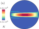
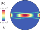
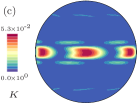
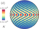
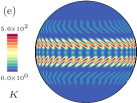
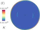
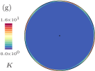
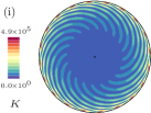
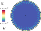
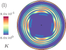
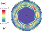
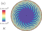
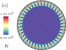
Figure 19: Modulated rotating wave with azimuthal symmetry $m_{2}=1$ in the case of the set $P_{3}$ (${\rm E}=3\times 10^{-7}$,${\rm Pr}=0.003$) at ${\rm Ra}=1.3030\times 10^{8}$. The contour plots for kinetic energy $K$ on a spherical section at $r\approx 0.99r_{o}$ (a-e), on an equatorial section (f-j), and on a colatitudinal section at $\theta=75^{\circ}$ (k-o). The $m=1,2,3,10,21$ azimuthal components of the solution are displayed in (a,f,k), (b,g,l), (c,h,m), (d,i,n), and (e,j,o), respectively.

The resonance conditions found for the azimuthal wave numbers $m\leq 14$, corresponding to the two MRWs at ${\rm Ra}=1.3030\times 10^{8}$ and at ${\rm Ra}=1.3919\times 10^{8}$, are listed in Table 3 and Table 4, respectively. The conditions, relating the largest peaks in the frequency spectrum $f_{m}$, are of two types. The first type corresponds to relations involving only low wave numbers $m\leq 5$ whereas the second type involves one low wave number and two moderate $6\leq m\leq 16$ wave numbers (see Table 3). In contrast, the relations for the second largest peak in the spectrum ($f^{2}_{m}$) can involve three moderate wave numbers (i.e $f_{13}=f^{2}_{6}+f_{7}$) since for the second peak the azimuthal wave number ordering is broken. For instance the modes $m\in\{4,5\}$ have $f_{m}$ in the small range but $f^{2}_{m}$ in the moderate range while the reverse occurs for $m=6$ (see Fig. 15). The quasiperiodic modes $m\in\{4,5\}$ are then dual in the sense that according to their first peak $f_{m}$ they may be classified as slow and according to their second peak $f^{2}_{m}$ the may be classified as moderate. The reverse occurs for $m=6$ and similarly for the moderate and fast modes. The situation for the MRW at ${\rm Ra}=1.3919\times 10^{8}$ is similar. In this case the kinetic energy of the nondominant azimuthal wave numbers is larger (see Fig. 12(c)) so more triadic resonant conditions due to nonlinear interactions are obtained (compare Table 3 with Table 4). At ${\rm Ra}=1.3919\times 10^{8}$ there are more dual quasiperiodic modes $m\in\{3,4,5,6,13,14,15,16,17\}$ and the modes corresponding to small, moderate, and large frequencies are now $m\leq 4$, $5\leq m\leq 14$, and $m\geq 15$.

Figure 16 displays the flow patterns, on a snapshot, corresponding to selected azimuthal modes with frequencies on each of the blocks of Fig. 15(a). Specifically, we select the azimuthal wave numbers $m=1$, $m=10$, and $m=21$ which correspond to slow, moderate, and fast purely periodic modes. The contour plots of the temperature perturbation (on equatorial and meridional sections), of the radial and azimuthal velocity (on an equatorial section), and of the vertical vorticity (on an equatorial section), are shown from left to right in each row (see figure caption). We note that only a single mode for each type (slow, moderate, or fast) is selected in Fig. 16 since the modes for each type have similar flow structure. Slow modes have vortices of $\Theta$ and $v_{r}$ located close to the origin of the sphere, with spiralling arms towards the outer boundary. In contrast, the situation for the flow structures is reversed. They are mainly attached to the outer sphere with spiralling arms towards the interior of the sphere (see $v_{\varphi}$ and $\hat{w}_{z}$ equatorial sections). For the moderate modes the vortices of $\Theta$ and $v_{r}$ are now located at a radial distance around $r_{o}/2$ so the spiralling arms towards the outer boundary are smaller. The flow structures are still mainly attached to the outer sphere but the spiralling arms now extend up to a radial distance around $r_{o}/2$. In contrast to this, the spiralling structures almost disappear in the case of the fast modes which have the vortices of $\Theta$ and $v_{r}$ located close to the outer boundary. The maximum flow velocities are not attached to the outer sphere, although remain very close to it (see equatorial section of $v_{\varphi}$).

The same contour plots as Fig. 16 are displayed in Fig. 17 corresponding to same azimuthal wave number decomposition of the Floquet eigenfunction of the RW with $m_{0}=11$ azimuthal symmetry at ${\rm Ra}=1.3011\times 10^{8}$ (already analyzed in Sec.III.1 and displayed in Fig. 6). The patterns are almost the same and make evident the relation between the resonant modes and the Floquet eigenfunctions. The eigenfunction, at ${\rm Ra}=1.3011\times 10^{8}$ close to the bifurcation point giving rise the MRW of Fig. 16, has dominant modes $m=1,10,12,21,23,..$, i.e, $m=1$ and $m=11k\pm 1$, $k\in\mathbb{Z}$ and the other modes have nearly zero velocity. When this spatial structure is coupled with the $m_{0}=11$ azimuthal symmetry of the unstable RW the main modes are $m=1$, $m=11k$, and $m=11k\pm 1$, $k\in\mathbb{Z}$ as exhibited by the MRW in Fig. 15(a) (also Fig. 12). It is interesting to note then that resonant modes arise due to the Hopf bifurcation giving rise to the MRW and that the Floquet eigenfunctions reveal the main structure of the resonant slow, moderate, and fast modes.

To further investigate the flow topology of slow and moderate modes Fig. 18 displays the equatorial sections of $\Theta$, $v_{r}$, and $v_{\varphi}$ for the azimuthal wave numbers $m=2,3,4,5$, and $m=6$. The former correspond to slow modes while the latter is a moderate mode. The main characteristic of this figure is that in the case of slow modes the spiraling arms form a polygonal structure to bound the interior of the sphere (this is best seen on the sections of $v_{\varphi}$). For the slow mode with $m=2$ the pattern is a square, for $m=3$ is an hexagon, etc. We note that the $m=2,3,4,5,6$ modes of Fig. 18 are negligible in the azimuthal wave number decomposition of the leading eigenfunction and thus are excited due to nonlinear interactions among the modes of the RW ($m=11k$, $k\in\mathbb{Z}$) and those of the eigenfunctions ($m=1$, $m=11k\pm 1$, $k\in\mathbb{Z}$). As the wave number is increased (from $m=2$ up to $m=5$) the vortices of $\Theta$ and $v_{r}$ of the slow modes tend to be located farther away from the interior and the spiraling arms of $v_{r}$ and $v_{\varphi}$ contain more cells. The patterns of the moderate mode, $m=6$, are changed significantly (compare with the slow mode $m=5$), especially for the case of $\Theta$ and $v_{r}$.

The azimuthal and latitudinal topology of the flow close to the outer sphere is displayed in the contour plots of the kinetic energy $K$ on a spherical surface of Fig. 19 (top row). In this figure the slow ($m=1,2,3$), moderate ($m=10$), and fast ($m=21$) modes are displayed from left to right. In the case of slow modes the convective motions are restricted to a relatively narrow belt surrounding the equator whereas for the moderate modes the convective vortices spiral in the azimuthal as well as latitudinal directions. For both types of modes the maximum value of $K$ is at the equator. In contrast, for the fast modes motions are almost forbidden at the equator but develop just above and below. The corresponding colatitudinal sections at the equator and at colatitude $\theta=75^{\circ}$ are displayed on the middle and bottom row, respectively. The equatorial sections now clearly show that in the case of the slow modes the motions are mainly attached to the outer boundary. However the bimodal nature of the flow, exhibiting interior polygonal structures of second order (notice the weak interior vortices for $m=1$ and $m=3$ at the equatorial plane) can be identified if the colatitudinal section does not intercept with the main vortices, for instance at $\theta=75^{\circ}$ (see bottom row of Fig. 19).

V Conclusions

We have performed a numerical study of thermal convection in an internally heated rotating sphere with very low Prandtl and Ekman numbers, appropriate for the study of planetary fluid cores. Concretely, three sets of parameters are considered $P_{1}=(\Pr,{\rm E})=(0.03,3\times 10^{-6})$, $P_{2}=(\Pr,{\rm E})=(0.01,10^{-6})$ and $P_{3}=(\Pr,{\rm E})=(0.003,3\times 10^{-7})$ which have already been studied in Kaplan et al. (2017). The focus of our investigation is on weakly nonlinear flows (weak branch of Kaplan et al. (2017)) occurring near the onset of convection, i. e. at weakly supercritical conditions ${\rm\widetilde{Ra}}={\rm Ra}/{\rm Ra_{c}}-1\leq 1$. By means of continuation methods (Keller (1977); Doedel and Tuckerman (2000); Sánchez and Net (2016)) we have computed branches of rotating waves (RWs), whose time dependence is described by a steady drift in the azimuthal direction, bifurcating directly from the base state. The stability analysis of RWs has evidenced that they are stable for all the models $P_{i}$. Additional direct numerical simulations (DNS) allow us to study secondary quasiperiodic flows (modulated rotating waves, MRWs) by analyzing Poincaré sections, kinetic energy spectra, and the time series of the flow and its individual modes.

The bifurcation diagrams of the Peclet number ${\rm Pe}$ of the RWs follow the $\sqrt{{\rm Ra}-{\rm Ra_{c}}}$ law for ${\rm\widetilde{Ra}}<3\times 10^{-2}$ since a Hopf bifurcation breaks the axisymmetry of the conduction state (Ecke et al. (1992)). In this interval the rotation frequencies $\omega$ of the RWs remain nearly constant. For larger values of ${\rm\widetilde{Ra}}$ the bifurcation diagrams become more complicated and can exhibit saddle-node points (as found for the model $P_{1}$). In contrast to Kaplan et al. (2017), we have been able to compute the weak branch for the model $P_{3}=(\Pr,{\rm E})=(0.003,3\times 10^{-7})$. The use of continuation methods helped us in this task since with DNS very long initial transients, about $30$ diffusion or $5\times 10^{4}$ rotation time units, are required before the nonlinear saturation of the solution. While steadily drifting solutions have neither been found in liquid gallium experiments nor numerical simulations of Horn and Schmid (2017); Aurnou et al. (2018); Vogt et al. (2021), we demonstrate that they can be found even with smaller ${\rm Pr}$ and ${\rm E}$. The existence of very long initial transients may make it unfeasible to detect them using experiments and require massive numerical simulations very close to the onset.

Our results show that for the lowest ${\rm E}$ and ${\rm Pr}$ considered (the set $P_{3}$) the RWs are of multicellular type as described in Net et al. (2008); Lin (2021) with azimuthal symmetry $m_{0}=12$ or $m_{0}=11$. A two-layer structure with some vortices of the kinetic energy ($K$) located close to the outer sphere and others located in the bulk of the fluid, displaying a polygonal pattern, is formed at the largest supercritical conditions studied, ${\rm\widetilde{Ra}}=1$. The present systematic computation of multicellular RWs complements the previous studies of Sánchez et al. (2013), considering a small inner core and at ${\rm E}=10^{-4}$ and ${\rm Pr}=0.1$, and Garcia et al. (2019), in the case of a very thin shell ($\eta=0.9$) at ${\rm E}=10^{-4}$ and ${\rm Pr}=0.003$. The study of Sánchez et al. (2013) corresponds to the systematic computation of RWs of spiralling type (e. g. Zhang (1992)), and that of Garcia et al. (2019) corresponds to RWs of polar type (described in Garcia et al. (2018)). In agreement with Sánchez et al. (2013); Garcia et al. (2019) RWs become unstable as a result of a supercritical Hopf bifurcation. We have found that for the set $P_{3}$ the analysis of stability of RWs is numerically challenging. This is because the eigenvalues are clustered near the unit circle, which degrades the convergence of eigenvalue solver, and means that multiple bifurcations take place near the onset (as in Garcia et al. (2019)). The analysis of the structure and symmetry $m_{1}$ of the eigenfunctions (Floquet modes) allows us to predict MRWs with azimuthal symmetry $m_{2}=1$.

The DNS presented here, starting from an unstable RW initial condition, exhibit strongly oscillatory and very long initial transients, about $30$ diffusion or $5\times 10^{4}$ rotation time units, before a weakly oscillatory quasiperiodic flow (MRW) is statistically saturated. This is because the perturbations grow very slowly in the unstable directions, given by Floquet modes, which are predicted by the stability analysis of RWs. Close to the bifurcation point the azimuthal wave number structure is inherited from the leading Floquet mode. The azimuthal wave number and time dependence of the long initial transients and the saturated solution is significantly different. Initial transients are characterized by strong time dependence and a large energy component of low azimuthal wave numbers $m<6$, whereas the kinetic energy spectra of the saturated solution are nearly constant in time and have significant peaks only for a reduced set of modes, including $m=1$. In addition, the time series of the temperature perturbation, at several points inside the sphere, reveal two very different time scales, slow and fast, associated to the interior ($r<r_{o}/5$) or the exterior ($r>r_{o}/2$) of the sphere, respectively. The former is characteristic of low wave numbers (e. g. $m=1$) whereas the latter is characteristic of moderate and large wave numbers (e.g. $m=11$).

As in Lin (2021) our DNS exhibit triadic resonances among different equatorially symmetric modes characterized by the spherical harmonic degree $l$ and order $m$, and in agreement with Garcia et al. (2021a) the solutions are MRWs. A characteristic block pattern with low, moderate, and large resonant wave numbers described by small, moderate, and large frequencies, respectively, is found in the frequency spectra. For the MRW closest to the bifurcation point these modes are $m\leq 5$, $6\leq m\leq 16$, and $m\geq 17$. The modes having largest peaks in the frequency spectrum are the non-vanishing components of the Floquet mode, $m=1$ and $m=11k\pm 1$, $k\in\mathbb{Z}$, which includes the $m=11$ mode of the parent RW.

The flow and temperature perturbation contour plots of the individual modes $m=1,10,21$ forming the leading Floquet eigenfunction are almost the same as the contour plots of the $m=1,10,21$ modes forming the resonant flow (MRW). For the slow modes (such as $m=1$) convective motions mainly occur close to the outer sphere (wall modes), on a narrow band around the equator. However, weak regular and polygonal structures (oval, square, hexagon) develop in the bulk of the fluid (interior modes) so the flow topology is of bimodal nature. The flow patterns of the $m=10$ moderate mode, although still attached to the outer sphere (wall modes) and with a maximum amplitude vortex at the equator, spiral to high latitudes and to the bulk of the fluid. In contrast, for the large mode $m=21$ the single vortex splits in two which are located symmetricaly above and below the equator, a little away from the outer boundary but without going deep into the interior. Either moderate ($m=10$) or large ($m=21$) modes have single mode structure since in this case there is no interior differentiated pattern.

While the patterns of RWs can be described by a single mode predicted by the linear stability analysis of the onset of convection, the patterns of MRWs can be multimodal and can be predicted by the stability analysis of RWs (periodic flows) and the computation of the leading Floquet modes. According to Lin (2021) (see introduction) the mechanism giving rise to the multimodal nature, i.  e. to flows from which dominant modes with different spatial localization can be identified (Horn and Schmid (2017); Aurnou et al. (2018); Vogt et al. (2021)), in the case of rotating convection at low ${\rm Pr}$ still remains a puzzle. Our study demonstrates that in this regime multimodal convection is generated by a Hopf bifurcaton of RWs (weak branch). Moreover, we have found that the specific spatial structure of the different spatially localized modes is determined by the stability analysis (Floquet modes) of the RWs.

VI Acknowledgements

This project has received funding from the European Research Council (ERC) under the European Union’s Horizon 2020 research and innovation programme (grant agreement No 787544). The authors kindly thank N. Schaeffer for his valuable comments.

References

- Glatzmaier and Roberts (1995) G.A. Glatzmaier and P.H. Roberts, “A three-dimensional self-consistent computer simulation of a geomagnetic field reversal,” Nature 377, 203–209 (1995).
- Schaeffer et al. (2017) N. Schaeffer, D. Jault, H.-C. Nataf, and A. Fournier, “Turbulent geodynamo simulations: a leap towards Earth’s core,” Geophys. J. Int. 211, 1–29 (2017).
- Heimpel et al. (2015) M. Heimpel, T. Gastine, and J. Wicht, “Simulation of deep-seated zonal jets and shallow vortices in gas giant atmospheres,” Nat. Geosci. 9, 19–23 (2015).
- Garcia et al. (2020) F. Garcia, F. R. N. Chambers, and A. L. Watts, “Deep model simulation of polar vortices in gas giant atmospheres,” Mon. Not. R. astr. Soc. 499, 4698–4715 (2020).
- Rüdiger (1989) G. Rüdiger, Differential Rotation and Stellar Convection: Sun and Solar-type Stars, Fluid mechanics of astrophysics and geophysics (Gordon and Breach Science Publishers, 1989).
- Brun et al. (2004) A. S. Brun, M. S. Miesch, and J. Toomre, “Global-Scale Turbulent Convection and Magnetic Dynamo Action in the Solar Envelope,” Astrophys. J. 614, 1073–1098 (2004).
- Jones (2007) C. A. Jones, “Thermal and compositional convection in the outer core,” Treat. Geophys. 8, 131–185 (2007).
- Gailitis et al. (2002) A. Gailitis, O. Lielausis, E. Platacis, G Gerbeth, and F. Stefani, “Colloquium: Laboratory experiments on hydromagnetic dynamos,” Rev. Mod. Phys. 74, 973–990 (2002).
- Moffatt and Dormy (2019) K. Moffatt and E. Dormy, Self-Exciting Fluid Dynamos, Cambridge Texts in Applied Mathematics (Cambridge University press, 2019).
- Dormy and Soward (2007) E. Dormy and A. M. Soward, eds., Mathematical Aspects of Natural Dynamos, The Fluid Mechanics of Astrophysics and Geophysics, Vol. 13 (Chapman & Hall/CRC, Boca Raton, FL, 2007).
- Julien et al. (2012) K. Julien, A. M. Rubio, I. Grooms, and E. Knobloch, “Statistical and physical balances in low Rossby number Rayleigh–Bénard convection,” Geophys. Astrophys. Fluid Dynamics 106, 392–428 (2012).
- Guervilly et al. (2019) C. Guervilly, P. Cardin, and N. Schaeffer, “Turbulent convective length scale in planetary cores,” Nature 570, 368–371 (2019).
- Christensen et al. (2001) U.R. Christensen, J. Aubert, P. Cardin, E. Dormy, S. Gibbons, G.A. Glatzmaier, E. Grote, Y. Honkura, C. Jones, M. Kono, M. Matsushima, A. Sakuraba, F. Takahashi, A. Tilgner, J. Wicht, and K. Zhang, “A numerical dynamo benchmark,” Phys. Earth Planet. Inter. 128, 25–34 (2001).
- Marti et al. (2014) P. Marti, N. Schaeffer, R. Hollerbach, D. Cébron, C. Nore, F. Luddens, J.-L. Guermond, J. Aubert, S. Takehiro, Y. Sasaki, Y.-Y. Hayashi, R. Simitev, F. Busse, S. Vantieghem, and A. Jackson, “Full sphere hydrodynamic and dynamo benchmarks,” Geophys. J. Int. 197, 119–134 (2014).
- Chandrasekhar (1981) S. Chandrasekhar, Hydrodynamic and Hydromagnetic Stability (Dover publications, inc. New York, 1981).
- Rand (1982) D. Rand, “Dynamics and symmetry. Predictions for modulated waves in rotating fluids,” Arch. Ration. Mech. Anal. 79, 1–37 (1982).
- Golubitsky et al. (2000) M. Golubitsky, V. G. LeBlanc, and I. Melbourne, “Hopf bifurcation from rotating waves and patterns in physical space,” J. Nonlinear Sci. 10, 69–101 (2000).
- Zhang (1992) K. Zhang, “Spiralling columnar convection in rapidly rotating spherical fluid shells,” J. Fluid Mech. 236, 535–556 (1992).
- Dormy et al. (2004) E. Dormy, A. M. Soward, C. A. Jones, D. Jault, and P. Cardin, “The onset of thermal convection in rotating spherical shells,” J. Fluid Mech. 501, 43–70 (2004).
- Zhang (1993) K. Zhang, “On equatorially trapped boundary inertial waves,” J. Fluid Mech. 248, 203–217 (1993).
- Net et al. (2008) M. Net, F. Garcia, and J. Sánchez, “On the onset of low-Prandtl-number convection in rotating spherical shells: non-slip boundary conditions,” J. Fluid Mech. 601, 317–337 (2008).
- Garcia et al. (2008) F. Garcia, J. Sánchez, and M. Net, “Antisymmetric polar modes of thermal convection in rotating spherical fluid shells at high Taylor numbers,” Phys. Rev. Lett. 101, 194501–(1–4) (2008).
- Garcia et al. (2018) F. Garcia, F. R. N. Chambers, and A. L. Watts, “The onset of low Prandtl number thermal convection in thin spherical shells,” Phys. Rev. Fluids 3, 024801 (2018).
- Sánchez et al. (2016) J. Sánchez, F. Garcia, and M. Net, “Critical torsional modes of convection in rotating fluid spheres at high taylor numbers,” J. Fluid Mech. 791 (2016), 10.1017/jfm.2016.52.
- Zhang et al. (2017) K. Zhang, K. Lam, and D. Kong, “Asymptotic theory for torsional convection in rotating fluid spheres,” Journal of Fluid Mechanics 813 (2017), 10.1017/jfm.2017.9.
- Ardes et al. (1997) M. Ardes, F. H. Busse, and J. Wicht, “Thermal convection in rotating spherical shells,” Phys. Earth Planet. Inter. 99, 55–67 (1997).
- Simitev and Busse (2003) R. Simitev and F. H. Busse, “Patterns of convection in rotating spherical shells,” New J. Phys 5, 97.1–97.20 (2003).
- Oruba and Dormy (2014) L. Oruba and E. Dormy, “Predictive scaling laws for spherical rotating dynamos,” Geophys. J. Int. 198, 828–847 (2014).
- Gastine et al. (2016) T. Gastine, J. Wicht, and J. Aubert, “Scaling regimes in spherical shell rotating convection,” J. Fluid Mech. 808, 690–732 (2016).
- Garcia et al. (2015) F. Garcia, J. Sánchez, E. Dormy, and M. Net, “Oscillatory convection in rotating spherical shells: Low Prandtl number and non-slip boundary conditions.” SIAM J. Appl. Dynam. Systems 14, 1787–1807 (2015).
- Horn and Schmid (2017) S. Horn and P. J. Schmid, “Prograde, retrograde, and oscillatory modes in rotating Rayleigh-Bénard convection,” J. Fluid Mech. 831, 182–211 (2017).
- Kaplan et al. (2017) E. J. Kaplan, N. Schaeffer, J. Vidal, and P. Cardin, “Subcritical Thermal Convection of Liquid Metals in a Rapidly Rotating Sphere,” Phys. Rev. Lett. 119, 094501 (2017).
- Lam et al. (2018) K. Lam, D. Kong, and K. Zhang, “Nonlinear thermal inertial waves in rotating fluid spheres,” Geophys. Astrophys. Fluid Dynamics 112, 357–374 (2018).
- Aurnou et al. (2018) J. M. Aurnou, V. Bertin, A. M. Grannan, S. Horn, and T. Vogt, “Rotating thermal convection in liquid gallium: multi-modal flow, absent steady columns,” J. Fluid Mech. 846, 846–876 (2018).
- Garcia et al. (2019) F. Garcia, F. R. N. Chambers, and A. L. Watts, “Polar waves and chaotic flows in thin rotating spherical shells,” Phys. Rev. Fluids 4, 074802 (2019).
- Lin (2021) Y. Lin, “Triadic resonances driven by thermal convection in a rotating sphere,” J. Fluid Mech. 909, R3 (2021).
- Massaguer (1991) J. M. Massaguer, “Stellar convection as a low Prandtl number flow,” in The Sun and Cool Stars: activity, magnetism, dynamos: Proceedings of Colloquium No. 130 of the International Astronomical Union Held in Helsinki, Finland, 17–20 July 1990, edited by I. Tuominen, D. Moss, and G. Rüdiger (Springer Berlin Heidelberg, 1991) pp. 57–61.
- Vogt et al. (2021) T. Vogt, S. Horn, and J. M. Aurnou, “Oscillatory thermal–inertial flows in liquid metal rotating convection,” J. Fluid Mech. 911, A5 (2021).
- Ecke et al. (1992) R. E. Ecke, F. Zhong, and E. Knobloch, “Hopf bifurcation with broken reflection symmetry in rotating Rayleigh-Bénard convection,” Europhys. Lett. 19, 177–182 (1992).
- Sánchez Umbría and Net (2019) J. Sánchez Umbría and M. Net, “Torsional solutions of convection in rotating fluid spheres,” Phys. Rev. Fluids 4, 013501 (2019).
- Keller (1977) H. B. Keller, “Numerical solution of bifurcation and nonlinear eigenvalue problems,” in Applications of Bifurcation Theory, edited by P. H. Rabinowitz (Academic Press, New York, 1977) pp. 359–384.
- Doedel and Tuckerman (2000) E. Doedel and L. S. Tuckerman, eds., Numerical Methods for Bifurcation Problems and Large-Scale Dynamical Systems, IMA Volumes in Mathematics and its Applications, Vol. 119 (Springer–Verlag, Berlin, 2000).
- Sánchez and Net (2016) J. Sánchez and M. Net, “Numerical continuation methods for large-scale dissipative dynamical systems,” Eur. Phys. J. Spec. Top. 225, 2465–2486 (2016).
- Garcia et al. (2016) F. Garcia, M. Net, and J. Sánchez, “Continuation and stability of convective modulated rotating waves in spherical shells,” Phys. Rev. E 93, 013119 (2016).
- Garcia et al. (2021a) F. Garcia, A. Giesecke, and F. Stefani, “Modulated rotating waves and triadic resonances in spherical fluid systems: The case of magnetized spherical couette flow,” Phys. Fluids 33, 044105 (2021a).
- Garcia et al. (2010) F. Garcia, M. Net, B. García-Archilla, and J. Sánchez, “A comparison of high-order time integrators for thermal convection in rotating spherical shells,” J. Comput. Phys. 229, 7997–8010 (2010).
- Sánchez et al. (2016) J. Sánchez, F. Garcia, and M. Net, “Radial collocation methods for the onset of convection in rotating spheres,” J. Comput. Phys. 308, 273–288 (2016).
- Orszag (1970) S. A. Orszag, “Transform method for calculation of vector-coupled sums: Application to the spectral form of the vorticity equation,” J. Atmos. Sci. 27, 890–895 (1970).
- Frigo and Johnson (2005) Matteo Frigo and Steven G. Johnson, “The design and implementation of FFTW3,” Proceedings of the IEEE 93, 216–231 (2005), special issue on ”Program Generation, Optimization, and Platform Adaptation”.
- Goto and van de Geijn (2008) Kazushige Goto and Robert A. van de Geijn, “Anatomy of high-performance matrix multiplication,” ACM Trans. Math. Softw. 34, 1–25 (2008).
- Crawford and Knobloch (1991) J. D. Crawford and E. Knobloch, “Symmetry and symmetry-breaking bifurcations in fluid dynamics,” Annu. Rev. Fluid Mech. 23, 341–387 (1991).
- Coughlin and Marcus (1992) K. T. Coughlin and P. S. Marcus, “Modulated waves in Taylor-Couette flow. Part 1. Analysis,” J. Fluid Mech. 234, 1–18 (1992).
- Kawahara et al. (2012) G. Kawahara, M. Uhlmann, and L. van Veen, “The signficance of simple invariant solutions in turbulent flows,” Arch. Ration. Mech. Anal. 44, 203–225 (2012).
- Hof et al. (2004) B. Hof et al., “Experimental observation of nonlinear traveling waves in turbulent pipe flow,” Science 305, 1594–1598 (2004).
- Doedel (1986) E. Doedel, AUTO: Software for continuation and bifurcation problems in ordinary differential equations, Report Applied Mathematics, California Institute of Technology, Pasadena, USA (1986).
- Sánchez et al. (2004) J. Sánchez, M. Net, B. García-Archilla, and C. Simó, “Newton-Krylov continuation of periodic orbits for Navier-Stokes flows,” J. Comput. Phys. 201, 13–33 (2004).
- Sánchez et al. (2013) J. Sánchez, F. Garcia, and M. Net, “Computation of azimuthal waves and their stability in thermal convection in rotating spherical shells with application to the study of a double-Hopf bifurcation,” Phys. Rev. E 87, 033014/ 1–11 (2013).
- Feudel et al. (2013) F. Feudel, N. Seehafer, L. S. Tuckerman, and M. Gellert, “Multistability in rotating spherical shell convection,” Phys. Rev. E 87, 023021–1–023021–8 (2013).
- Feudel et al. (2015) F. Feudel, L. S. Tuckerman, M. Gellert, and N. Seehafer, “Bifurcations of rotating waves in rotating spherical shell convection,” Phys. Rev. E 92, 053015 (2015).
- Tuckerman et al. (2019) L. S. Tuckerman, J. Langham, and A. Willis, “Order-of-magnitude speedup for steady states and traveling waves via stokes preconditioning in channelflow and openpipeflow,” in Computational Modelling of Bifurcations and Instabilities in Fluid Dynamics (Springer International, Cham, Switzerland, 2019) pp. 3–31.
- Jordan and Smith (2007) D. Jordan and P. Smith, Nonlinear Ordinary Differential Equations : An Introduction for Scientists and Engineers, Oxford Texts in Applied and Engineering Mathematics, Vol. 10 (Oxford University Press, 2007).
- Lehoucq et al. (1998) R. B. Lehoucq, D. C. Sorensen, and C. Yang, ARPACK User’s Guide: Solution of Large-Scale Eigenvalue Problems with Implicitly Restarted Arnoldi Methods (SIAM, 1998).
- Tuckerman (2015) L. S. Tuckerman, “Laplacian preconditioning for the inverse Arnoldi method,” Commun. Comput. Phys. 18, 1336–1351 (2015).
- Saad (1992) Y. Saad, Numerical Methods for Large Eigenvalue Problems (Manchester University Press, Manchester, 1992).
- Garcia et al. (2014) F. Garcia, E. Dormy, J. Sánchez, and M. Net, “Two computational approaches for the simulation of fluid problems in rotating spherical shells,” in Proc. of the 5th International Conference on Computational Methods - ICCM2014. Cambridge, England, Vol. 1, edited by G. R. Liu and Z. W. Guan (2014).
- Marcus and Tuckerman (1987) P. S. Marcus and L. S. Tuckerman, “Simulation of flow between concentric rotating spheres. Part 1. Steady states,” J. Fluid Mech. 185, 1–30 (1987).
- Barik et al. (2018) A. Barik, S. A. Triana, M. Hoff, and J. Wicht, “Triadic resonances in the wide-gap spherical Couette system,” J. Fluid Mech. 843, 211–243 (2018).
- Laskar (1993) J. Laskar, “Frequency analysis of a dynamical system,” Celestial Mech. Dyn. Astron. 56, 191–196 (1993).
- Garcia et al. (2021b) F. Garcia, M. Seilmayer, A. Giesecke, and F. Stefani, “Long term time dependent frequency analysis of chaotic waves in the weakly magnetised spherical Couette system,” Physica D 418, 132836 (2021b).