Network Graph Based Neural Architecture Search

Abstract

Neural architecture search enables automation of architecture design. Despite its success, it is computationally costly and does not provide insight on how to design a desirable architecture. Here we propose a new way of searching neural network where we search neural architecture by rewiring the corresponding graph and predict the architecture performance by graph properties. Because we do not perform machine learning over the entire graph space and use predicted architecture performance to search architecture, the searching process is remarkably efficient. We find graph based search can give a reasonably good prediction of desirable architecture. In addition, we find graph properties that are effective to predict architecture performance. Our work proposes a new way of searching neural architecture and provides insights on neural architecture design.

1 Introduction

Neural networks architecture achieves a great success over last few years in various challenging applications, such as image classification Krizhevsky et al. (2012), speech recognition Hinton et al. (2012) and machine translation Wu et al. (2016). The success, largely attributed to the feature engineering, is accompanied by the arise of architecture engineering, e.g., AlexNet Krizhevsky et al. (2012), VGGNet Simonyan and Zisserman (2014), ResNet He et al. (2016). Increasingly complicated neural network architectures make it progressively more difficult for manual design of architecture. Neural architecture search (NAS), enabling automation of architecture engineering, proves its potential in boosting the performance of neural network architecture. For example, NAS methods have outperformed some manually designed architecture in some applications, such as image classification Real et al. (2019), object detection Zoph et al. (2018).

In NAS method, there are three major components Elsken et al. (2019): search space $\mathcal{S}$, search strategy ${\mathcal{A}}_{s}$ and performance estimation strategy ${\mathcal{A}}_{e}$. Predefined $\mathcal{S}$ confines the total number of possible architectures if it is not unbounded. Thus it will affect the search efficiency and optimal architecture. ${\mathcal{A}}_{s}$ determines the search efficiency and should avoid potential pitfall of local minimum. ${\mathcal{A}}_{e}$ provides a way to evaluate architecture candidate and feedback. The simplest way for ${\mathcal{A}}_{e}$ is to perform a standard training and validation for targeting optimal architecture.

Powerful as NAS method is, searching an architecture in $\mathcal{S}$ and testing its performance will take ample time. Although decomposing hand-crafted architectures into motifs and searching motifs, blocks or cells can boost searching speed, this process inevitably introduces bias in the search space. Furthermore, NAS method does not throw light on why specific architectures outperform others and general principles of designing an architecture. Network graphs, on the other hand, have good metrics for evaluation. For example, clustering coefficient measures the degree to which nodes a in graph cluster. If we can bridge graph and neural network, we will be able to relate graph properties to architecture performance. Instead of searching in architecture space, we can perform search in graph space. By targeting the optimal graph structure, we will able to locate the optimal neural network architecture.

Figure 1 shows the graph-based neural architecture search. The relationship between graph and neural network is bridged by relational graph. We predict machine learning error based on graph properties. A set of graph features is selected for the prediction. Based on predicted error, we apply rewiring strategy to search a better or worse neural architecture.

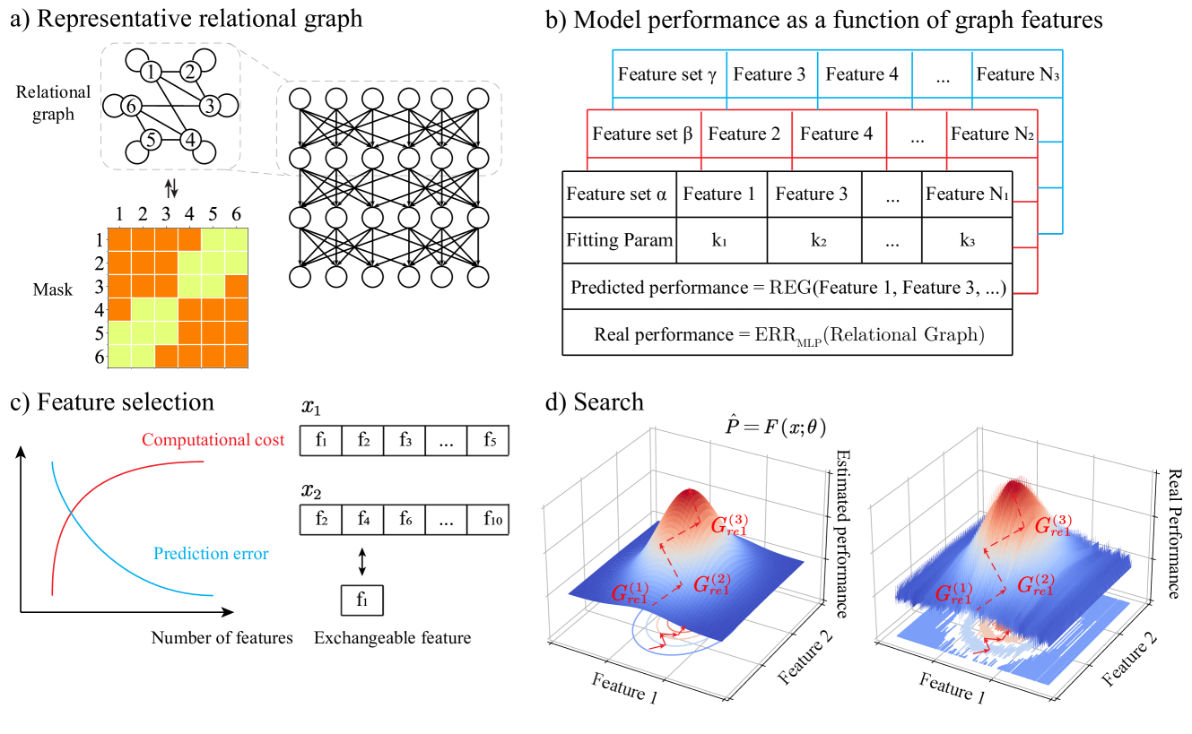
Figure 1: Schematic illustration of graph-based neural architecture search

2 Bridge of Neural Network and Graph

2.1 Graph Representation of Neural Network

The relation between graph and neural network can be bridged by relational graph You et al. (2020). For a fixed-width multilayer perceptron (MLP) where each layer contains the same number $R$ of computation units (neurons), suppose the input and output of the $r$-th layer ($1\leq r\leq R$) is $\mathbf{X}^{(r)}$ and $\mathbf{X}^{(r+1)}$, respectively. A neuron in the $r$-th layer computes You et al. (2020):

$$x^{(r+1)}_{i}=\sigma(\sum_{j\in N(i)}\omega^{(r)}_{ij}x^{(r)}_{j}),$$ (1)

where $w^{(r)}_{ij}$ is the $i$-th row and $j$-th column of the trainable weight $\mathbf{W}^{(r)}$, $x^{(r)}_{j}$ is the $j$-th dimension of the input $\mathbf{X}_{j}$, $x^{(r)}_{i}$ is the $i$-th dimension of the output $\mathbf{X}_{i}$. $\sigma(\cdot)$ is the activation function introducing non-linearity. $N(i)$ is the set of neurons of the $(r+1)$-th layer connecting to $r$-th layer and defined by relational graph $G$.

2.2 Undirected Graph Generator

Graphs can be categorized into two groups: directed graph or undirected graph. We consider relational graph as undirected, so its adjacency matrix is symmetric. The classic graph generation algorithms include (1) Watts-Strogatz (WS) model that can generate graphs with small-world properties Watts and Strogatz (1998). The ”small world effect” is generally referred to describe graphs whose average path length is comparable with a homogeneous random graphs Prettejohn et al. (2011); (2) Erdős-Rényi (ER) model that can generate random graphs Erdos et al. (1960); (3) Barabási-Albert (BA) model that constructs scale-free graphs Barabási and Albert (1999). A scale-free graph has a degree distribution following power law, i.e., the probability of a node having a degree $k$ has a scale-invariant decay $P(k)\sim k^{-\gamma}$, where $\gamma$ is a constant and confined by $\gamma>1$; (4) Harary model that generates graphs with maximum connectivity Harary (1962). WS-flex graph generator, proposed in You et al. (2020), is a more general form of WS model by relaxing the constraint that all the nodes have the same degree before random rewiring. After fixing the number of nodes to be 64, WS-flex graph generators are capable of generating graphs encompassing almost all graphs constructed by classic graph generation algorithms mentioned above You et al. (2020).

3 Experimental Setup

We use the CIFAR-10 dataset Krizhevsky et al. (2009) for training MLPs. CIFAR-10 dataset has 50K training images and 10K validation images. Each image is a matrix with a dimension of $32\times 32\times 3$. 60K images are classified into 10 categories for supervised machine learning.

3.1 Graph Space

We use WS-flex graph generator to generate undirected graphs. The number of nodes is fixed to be $64$ and the average degree range is $[2,63]$. Total number of generated graphs is $5983$. We calculate $26$ Graph properties including average degree, clustering coefficient, heterogeneity, average path length, bimodularity, greedy modularity, resilience parameter, degree entropy, wedge count, gini index, average node connectivity, edge connectivity, average closeness centrality, average closeness centrality (WF improvement), average eccentricity, diameter, radius, average edge betweenness centrality, average node betweenness centrality, central point of dominance, core number, minimum Laplacian spectrum, maximum Laplacian spectrum, transitivity, local efficiency, global efficiency. Detailed description regarding to those properties can be referred in Appendix A.

We find that heterogeneity range for $5983$ graphs constructed by ws-flex graph generator is $[0,0.82]$. Most graphs are not heterogeneous in the structure. To introduce more heterogeneous graphs, we do random rewiring based on those graphs. Total number of graphs becomes $19724$.

3.2 Feature Selection

Average path length and clustering coefficient are considered as good indicator for predicting learning error of MLP You et al. (2020). We calculate 28 features for each graph and take into consideration the potential of these features for predicting machine learning performance. To filter features, we use sequential forward selection (SFS) algorithm Marcano-Cedeño et al. (2010); Ververidis and Kotropoulos (2005); Cotter et al. (1999), a commonly used method for reducing the data dimension. SFS algorithm is a bottom-up search strategy in which an empty set $S$, the starting point, continuously add features until all features are added. At each iteration, $S$ greedily searches for best feature from remaining feature pool and include it.

Selecting MLP learning error as output variable and graph properties as input variables, We use linear regression to fit results and choose mean squared error (MSE) as metric to select features. We use random splitting strategy to obtain training set and test set. The ratio of training set to test set is $9:1$. At each iteration of SFS algorithm, we use training set to determine linear regression parameters and test set to calculate evaluation parameters MSE and Pearson correlation coefficient.

3.3 Neural Network Architecture

We use a 5-layer MLPs as the neural network architecture. Each MLP layer has 512 hidden units as baseline architecture. The relational graph determines the connection of hidden units between two neighboring layer. To ensure all networks have the approximately same complexity, we use FLOPS (# of multiplication and addition) as metric to adjust baseline architecture such that FLOPS for different relational graph represented networks is roughly the same.

Fig. 1 a) shows the illustration of MLP architecture. Each MLP layer contains Batchnorm ReLU layer to introduce non-linearity and BatchNorm layer Ioffe and Szegedy (2015). Batch size in the training process is 128 and total number of epochs for training a model is 200. We use a decaying learning rate with a cosine annealing Loshchilov and Hutter (2016). Our Momentum Optimizer has an initial learning rate of 0.1, 5e-4 weight decay, 0.9 momentum and uses Nesterov Momentum Sutskever et al. (2013); Nesterov (1983).

3.4 Rewiring Algorithm

To search the best neural architecture, we adopt a greedy strategy which is different from the conventional approaches in NAS. We start from a neural architecture with known performance, improving the architecture by iteratively rewiring it. Let $G_{t}$ be the current architecture, $P(G_{t})$ be the post-training performance of $G_{t}$, and $\mathcal{A}$ be our rewiring strategy, we can formulate the rewiring procedure as

$$G_{t+1}=\operatorname*{arg\,max}_{\mathcal{A}}P(\mathcal{A}(G_{t})).$$ (2)

Nevertheless, training each $\mathcal{A}(G_{t})$ for the performance $P(\mathcal{A}(G_{t}))$ will make the search inevitably expensive. To address this issue, we refer to a surrogate parametric model $F(G;\bm{\theta})$ for $P(G)$, which is designed to capture the relationship between a set of simple topological properties (see Appendix A) and the performance of $G_{t}$, i.e. $\hat{P}(G)=F(G;\bm{\theta})$. To some extend, the “goodness” of $F$ determines our choices of the resultant architectures via rewiring. We search the architecture by selecting a good rewired candidate or discarding a bad one. If $F(G_{t};\bm{\theta})$ is consistent with the real performance $P(G_{t})$, there will be very few mistakes in our choices and our search will guarantee a constantly improved architecture. Also, some architectures may be a local optimal, which can not be rewired to reach a better one.

As shown in Algorithm 1, our approach starts from a randomly selected relation graph whose associated neural network post-trained performance may be arbitrarily low. We perform a greedy search of a sequence of rewiring operations to constantly improve the performance of the associated neural network of the initial relational graph. Currently, our rewiring strategy allows removal of edges $\mathcal{A}_{\rm rmv}$, building new edges $\mathcal{A}_{\rm new}$, random rewiring $\mathcal{A}_{\rm rnd}$ and double edge swaps $\mathcal{A}_{\rm swap}$.

Algorithm 1 Rewiring and Searching

Input: A randomly selected relation graph $G_{0}\in\mathcal{G}$, four rewiring operations $\{\mathcal{A}_{\rm new},\mathcal{A}_{\rm rmv},\mathcal{A}_{\rm swap},\mathcal{A}_{\rm rnd}\}$, accepted relative improvement $\varepsilon\in(0,1)$, maximum number $K$ of rewiring operations, the performance predictor $F(G;\bm{\theta})$ of the associated neural network $\phi(G)$ with the topological properties of a relational graph $G$
Output: Rewired relation graph $G_{K}$

1:  Let $k=0$, $\hat{P}_{0}=F(G_{0};\bm{\theta})$.

2:  while $k<K$ do

3:     Randomly select a rewiring operation $\mathcal{A}$

4:     Perform $\mathcal{A}$ over $G_{k-1}$ and obtain $\hat{G}_{k-1}=\mathcal{A}(G_{k-1})$

5:     Predict the post-trained performance of $\phi(\hat{G}_{k-1})$ with $\hat{P}_{k}=F(\hat{G}_{k-1};\bm{\theta})$

6:     if $|\hat{P}_{k}/\hat{P}_{k-1}-1|\geq\varepsilon$ then

7:        Accept $\mathcal{A}$ with $G_{k}=\hat{G}_{k-1}$ and set $k=k+1$

8:     else

9:        Reject $\mathcal{A}$ and repeat the above procedure

10:     end if

11:  end while

4 Experimental Result

4.1 Features for prediction

Calculating all features of a graph can be computational expensive. Hence, we are interested in how many features are needed to predict MLP performance and what are important features. We use SFS algorithm to quantitatively show the relation between number of features and prediction quality, as well as to determine significant features.

Figure 2 shows MSE and Pearson correlation coefficient variation with including features. Instead of typical oscillating trend of SFS algorithm, MSE shows a monotone decreasing with adding features. Even though more features give a better prediction quality, the gain in prediction boost becomes negligible while the computational cost increases dramatically when the number of features is more than $10$. At the same time, we find linear regression can give a good prediction. If we only choose one feature, MSE is $0.086$. Adding just $4$ more features, MSE drops to $55\%$ that of one feature. Considering the trade-off between prediction performance and computation cost, we choose the first 10 features to predict MLP learning error. The corresponding MSE is $0.4$ and we have a high $0.93$ Pearson correlation coefficient. The finding suggests that a small number of features can still give a good prediction of MLP performance.

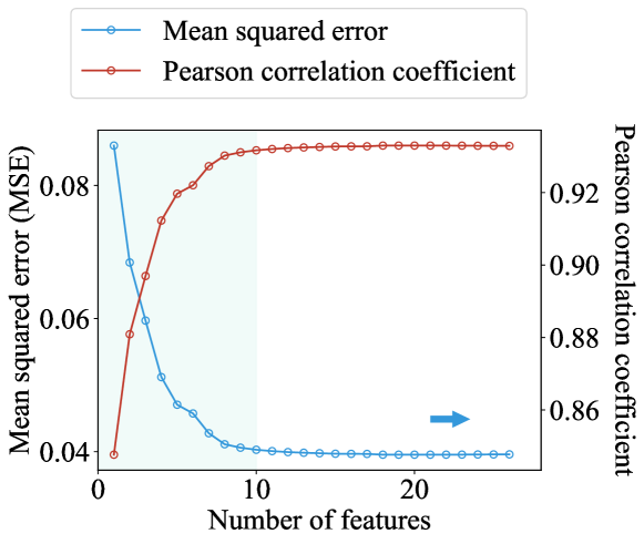
Figure 2: Sequential forward selection for feature selection

SFS algorithm determines the eccentricity as the starting point. We are interested, within a certain tolerance on prediction error of MLP performance, can we choose other features as starting point that give a similar prediction quality? There are several benefits for moderately sacrificing prediction quality: 1) the computational cost for different features can vary a lot. If we replace features having a high computational cost with ones having low cost and, at the same time, the prediction quality does not change much, the MLP prediction model will be satisfying; 2) there are highly developed theories about some of features. If we use those features for prediction, it is beneficial to understand why and how a neural network has a good performance. For example, the eccentricity measures the maximum distance from one node to all other node. The average path length measures the average of minimum distance between all pairs of nodes. These two features are closely related to message exchange efficiency. If we can replace the eccentricity with the average path length, we will be able to analyze neural network performance using the average path length related theories, e.g., small world network theory; 3) in reality, it is unlikely a certain rewiring strategy just alters one graph property while other property remains unchanged. If we can replace less controllable feature with more controllable one, it becomes easier to target optimal relational graph.

We replace the first feature, i.e., eccentricity, with other features and perform SFS algorithm to determine remaining features. Figure 3 shows representative MSE variation as a function of number of features in SFS algorithm after fixing the first feature. Generally, a different starting point of SFS algorithm will lead to different feature set $S$ and different MSE. However, some features give a similar prediction quality and feature set. For example, MSE for average path length and eccentricity at each iteration is very close. Besides, the order of adding features is nearly the same. When we consider the first $10$ features excluding first feature, the eccentricity and the average path length have the same remaining $9$ features. The feature adding order is also the same.

When a single feature is used for predicting MLP performance, calculated features have a pronounced difference in the prediction quality. Some features, such as heterogeneity, have a high $0.3$ MSE. Nevertheless, with adding more features, all features show a fast converge (adding less than 10 features) to a small $0.4$ MSE. This indicates that a linear combination of features gives a good prediction of MLP performance. More details about MSE variation with adding features when fixing the first feature can be referred in Appendix C.

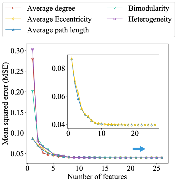
Figure 3: Representative sequential forward selection after fixing the first feature

Table 1 shows first $10$ features determined by SFS algorithm and first $10$ features by SFS algorithm after fixing first feature to be the average path length. Except the first feature, two feature sets have the exactly the same features and linear regression parameters associated with these features have the same sign, i.e., consistent positive correlation or negative correlation. In addition, MSE is close for these two feature sets. Hence, we think the average eccentricity and average path length are interchangeable in terms of predicting MLP performance.

Algorithm	Selected Features	Sign
SFS	Average eccentricity	$+$
	Central point of dominance	$+$
	Resilience Parameter	$+$
	Global efficiency	$-$
	Edge connectivity	$-$
	Wedge count	$-$
	Clustering coefficient	$-$
	Average node connectivity	$+$
	Average closeness centrality	$+$
	Greedy modularity	$-$
	Average path length	$+$
	Central point of dominance	$+$
	Resilience Parameter	$+$
	Global efficiency	$-$
SFS fixing	Edge connectivity	$-$
first feature	Wedge count	$-$
	Clustering coefficient	$-$
	Average node connectivity	$+$
	Average closeness centrality	$+$
	Greedy modularity	$-$

Table 1: Feature sets determined by SFS algorithms

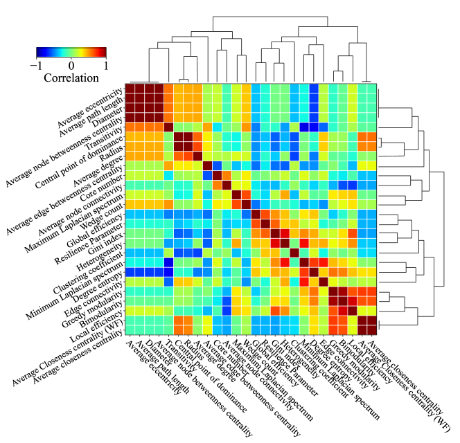
Figure 4: Pearson correlation coefficient of every pair of graph features. Feature sets related to every feature are determined by SFS algorithm

Except for the pair of the average eccentricity and average path length, we are also curious about a question – are there other features interchangeable. We use Pearson correlation coefficient to characterize the similarity between every pair of feature sets. We fix first feature and use SFS algorithm to determine the remaining $9$ features. Every remaining $9$ features constitute a set $S$. Then we calculate Pearson correlation coefficient between pairs of those sets. Figure 4 shows Pearson correlation coefficient between all pairs of features. The result reveals the similar effect in predicting MLP performance. The similarity seems to be correlated to physical meaning of graph features. For example, the average path length measures the average of shortest path length between pairs of nodes Albert and Barabási (2002); Achard and Bullmore (2007). The average eccentricity measures the maximum distance from one node to other nodes in a graph $G$ Hage and Harary (1995). Diameter is the maximum eccentricity of a graph $G$. Average node betweenness centrality calculates the average of node betweenness centrality which is the sum of the fraction of all shortest paths passing through a node Brandes (2001, 2008). These four features are related to message exchange efficiency in a graph. At the same time, they have a highest correlation 1.

4.2 Prediction of MLP performance

We choose as the starting point a graph with a highest MLP top 1 error and a graph with lowest MLP top 1 error in the graph pool. Then we use the rewiring strategy described before to rewire graph for searching a better graph structure step by step. At each iteration, if the predicted error decreases by more than a threshold value $0.01$, the rewired graph is accepted and the change of graph structure due to rewiring is kept. To verify the prediction of performance, we use MLPs represented by relational graphs at each stage to calculate the real top 1 error. Total time for rewiring is $6$ hours.

Figure 5 shows the top 1 error decrease path (superior rewiring) and Figure 6 shows the top 1 error increase path (inferior rewiring). At the end of the rewiring process, both superior rewiring and inferior rewiring show a dramatic increase in the computational cost. In both rewirings, real top 1 error oscillates around the predicted top 1 error. The prediction is promising as the real top 1 error overall follows the prediction path. During the rewiring process, we do not observe the sudden jump in the top 1 error. We think that limited change in the graph edge set does not change MLP performance dramatically. This is consistent with the result from conventaional NAS: small perturbations in the neural network architecture does not have a significant effect on its performance Ru et al. (2020). During the superior rewiring process, the computational cost increases drastically even though the learning error does not hit the minimal error region. This might be attributed to premature convergence to the region of suboptimal structure. There seems to be a exploration-exploitation trade-off problem. The greedy searching strategy might lead to a suboptimal graph structure.

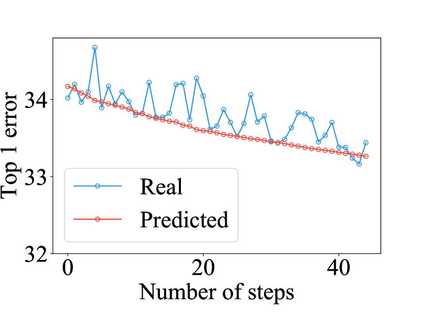
(a) Top 1 error decrease path

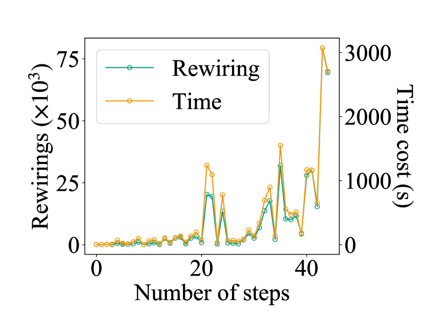
(b) Computational cost

Figure 5: Rewiring path of MLP learning error decrease

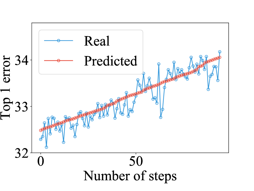
(a) Top 1 error increase path

(b) Computational cost

Figure 6: Rewiring path of MLP learning error decrease

We choose the graph in inferior rewiring as the starting point and repeat our rewiring strategy for 100 times. We use 100 random seeds to generate different random rewiring processes. Figure 7 shows the statistical result of rewiring result. We select continuous step periods, e.g., step 1 to step 10 as one step range and then step 11 to step 20 as another step range. Then we calculate the average of real MLP top 1 errors of each step range. As the number of rewiring steps increases, the median number of average top 1 error increases. This trend is consistent with our prediction, i.e., the statistical increase in top 1 error has a same trend as the predicted increase in top 1 error. Hence, the performance predictor $F(G;\bm{\theta})$ can be used for predicting MLP performance.

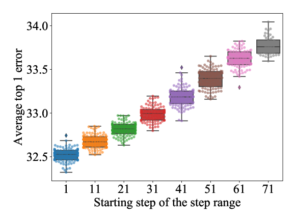
Figure 7: Statistical result of rewiring path

5 Discussion

The performance of neural network architecture can be related to properties of corresponding relational graph. For example, the average path length is a measurement of efficiency of information transport over a graph. At the same time, it is a good indicator of MLP performance. In general, a lower average path length is preferred over a higher one (refer to A). However, there is no continuous function fitting well a single graph property and MLP performance. It is impractical to just rely on one graph feature to predict MLP performance. A combination of graph properties, nevertheless, can give a reasonably good prediction of the performance. By predicting a learning error, we are able to search an optimal neural network architecture just by rewiring a graph and calculating graph properties. The benefit of avoiding performing machine learning over an entire graph space is high time efficiency and low computational cost. We adopt linear regression to calculate predicted performance based on graph properties, this process is computationally cheap. Because the graph space is unbounded and does not rely on typical manual designed architecture, the search space is unbiased. Overal, the real MLP performance is consistent with the predicted MLP performance. Based on predicted MLP performance, we are able to target inferior or superior graph structure.

We find different properties might have a similar effect in machine learning accuracy. In other words, some properties are interchangeable. The interchangeability is consistent to physical meaning of those properties. For instance, the average path length, diameter and eccentricity are all related to message exchange efficiency. They are interchangeable in terms of predicting machine learning performance. A directed rewiring strategy, targeting at changing a specific group of graph properties, will definitely enhance the search efficiency.

Appendix A Features of a Graph Network

Average degree. The average degree $\bar{k}$ calculates the average number of edges for one node Luce and Perry (1949). For a graph with $n$ nodes, the average degree $\bar{k}$ is given by:

$$\bar{k}=\frac{\sum_{i\in N}k_{i}}{n},$$ (3)

where $1\leq i\leq n$ and $k_{i}$ is the degree of node $i$. For a complete undirected graph, the average degree is $n-1$.

Clustering coefficient. The clustering coefficient describes the likelihood of a node $j$ in the neighborhood $N_{i}$ of node $i$, is immediately connected to other nodes in $N_{i}$ Watts and Strogatz (1998). The clustering coefficient $C_{i}$ for node $i$ in an undirected graph is given by:

$$C_{i}=\frac{|\{e_{jk},j\in N_{i},k\in N_{i},e_{jk}\in E,j\neq k\}|}{\begin{pmatrix}k_{i}\\ 2\end{pmatrix}},$$ (4)

where $e_{jk}$ is the edge connecting node $j$ and $k$, $E$ is the set of edges for graph $G$. Notation $|\{e_{jk},j\in N_{i},k\in N_{i},e_{jk}\in E,i\neq j\}|$ represents the number of edges within the neighbourhood of node $i$. A larger clustering coefficient physically means nodes in a graph are more likely to cluster together. We use the average clustering coefficient $\frac{1}{n}\sum_{i\in N}C_{i}$ as clustering coefficient $C$ of a graph.

The heterogeneity $\mathcal{H}$ of an unweighted graph is the ratio of variance of degree $k$ to expectation of $k$ and given by Gao et al. (2016):

$$\mathcal{H}=\frac{\frac{1}{n}\sum_{i\in N}k_{i}^{2}-(\frac{1}{n}\sum_{i\in N}k_{i})^{2}}{\frac{1}{n}\sum_{i\in N}k_{i}}$$ (5)

For a graph with homogeneous degree distribution, heterogeneity is equal to 0.

The average path length $\bar{l}$ measures the average distance between any two nodes in the network and is defined by sum of shortest path length between all pairs of nodes normalized by the total number of node pairs Albert and Barabási (2002); Achard and Bullmore (2007):

$$\bar{l}=\frac{\sum_{i,j\in N,i\neq j}l_{i,j}}{n(n-1)}$$ (6)

Where $l_{i,j}$ is the shortest path length between node $i$ and $j$. The average path length measures the efficiency of message passing over a graph.

The modularity describes the quality of partition of a graph into communities. A good partition separates nodes in such way that majority of edges is in communities and minority lies between them Clauset et al. (2004); Newman and Girvan (2004). The modularity $Q$ is defined by:

$$Q=\frac{1}{2n}\sum_{i,j\in N}(A_{ij}-\frac{k_{i}k_{j}}{2n})\delta(c_{i},c_{j})$$ (7)

Where $A$ is the adjacency matrix of a graph $G$, the $\delta$-function $\delta(c_{i},c_{j})$ is 1 if $i$ and $j$ are in the same community 0 otherwise. Bimodularity $Q_{b}$ measures the quality of partitioning a graph into two blocks using the Kernighan-Lin algorithm. Kernighan-Lin algorithm partitions nodes of a graph in the manner of minimizing the costs on cutting edges. Greedy modularity $Q_{g}$ measures the quality of partitioning nodes using Clauset-Newman-Moore greedy modularity maximization Clauset et al. (2004).

The resilience parameter $\beta_{\text{eff}}$ of an undirected graph is given by Gao et al. (2016):

$$\beta_{\text{eff}}=\frac{\frac{1}{n}\sum_{i\in N}k_{i}^{2}}{\frac{1}{n}\sum_{i\in N}k_{i}}$$ (8)

The physical meaning of resilience is the ability of a system to maintain basic functionality after external perturbation.

The degree entropy $H$, a measure of disorder, calculates the entropy of the degree distribution and is given by Ji et al. (2021):

$$H=\frac{1}{n}\sum_{i\in N}-\frac{k_{i}}{m}\log\frac{k_{i}}{m}$$ (9)

Where $m$ is the total number of edges.

The wedge count $W$ counts the number of wedge that is defined as a two-hop path in an undirected graph. $W$ can be calculated by Ji et al. (2021); Gupta et al. (2016):

$$W=\sum_{i\in N}\begin{pmatrix}k_{i}\\ 2\end{pmatrix}$$ (10)

The Gini index $\mathcal{G}$ measures sparsity of a graph and is defined by Goswami et al. (2018); Ji et al. (2021):

$$\mathcal{G}=\frac{2\sum_{i\in N}i\hat{k}_{i}}{n\sum_{i\in N}\hat{k}_{i}}-\frac{n+1}{n}$$ (11)

Where $\hat{k}_{i}$ is the degree of node i after sorting degrees.

The average node connectivity $\bar{\kappa}$ is the average of local node connectivity over all pairs of nodes of a graph $G$ and defined as Beineke et al. (2002):

$$\bar{\kappa}=\frac{\sum_{i,j\in N,i\neq j}\kappa(i,j)}{\begin{pmatrix}n\\ 2\end{pmatrix}}$$ (12)

Where $\kappa(i,j)$ is defined as the maximum value of $\kappa$ for which node $i$ and $j$ are $\kappa$-connected. For node $i$ and $j$ considered as $\kappa$-connected, there are $\kappa$ or more pairwise internally disjoint paths between them.

The edge connectivity is the minimum number of edges needed in order to disconnect a graph $G$ Esfahanian (2013).

The closeness centrality $\mathcal{C}_{i}$ for a node $i$ is the reciprocal of the average shortest path length $l$ of node $i$ to all other $n_{r}-1$ nodes Freeman (1978):

$$\mathcal{C}_{i}=\frac{n_{r}-1}{\sum_{j\in N,j\neq i}l_{i,j}}$$ (13)

The improved closeness centrality $\mathcal{C}_{i}^{WF}$ by Wasserman and Faust adds a scale factor to scale down closeness centrality for unconnected graph and is given by Wasserman et al. (1994):

$$\mathcal{C}_{i}^{WF}=\frac{n_{r}-1}{n-1}\frac{n_{r}-1}{\sum_{j\in N,j\neq i}l_{i,j}}$$ (14)

For a connected graph, there is no difference between the close centrality $\mathcal{C}_{i}$ and the improved closeness centrality $\mathcal{C}_{i}^{WF}$.

The eccentricity is defined as the maximum distance from node in a graph to all other nodes Hage and Harary (1995). The diameter of a graph is the maximum eccentricity while the radius of a graph is the minimum eccentricity.

The average edge betweenness centrality calculates the average of betweenness centrality $\mathcal{C}_{B}(e_{k})$ for all edges of a graph. The betweenness centrality for an edge $e_{k}$ is the sum of the fraction of all shortest paths passing through $e_{k}$. The betweenness centrality can be calculated by Brandes (2001, 2008):

$$\mathcal{C}_{B}(e_{k})=\sum_{i,j\in N,i\neq j}\frac{\sigma_{i,j}\bigr{\rvert}_{e_{k}}}{\sigma_{i,j}}$$ (15)

Where $\sigma_{i,j}$ is the number of shortest paths connecting node $i$ and $j$. $\sigma_{i,j}\bigr{\rvert}_{e_{k}}$ is the number of those paths passing through edge $e_{k}$.

Similar to the average edge betweeness centrality, the average node betweenness centrality calculates the average of betweenness centrality $\mathcal{C}_{B}(n)$ for all nodes of a graph. $\mathcal{C}_{B}(n)$ is expressed as:

$$\mathcal{C}_{B}(k)=\sum_{i,j\in N,i\neq j}\frac{\sigma_{i,j}\bigr{\rvert}_{k}}{\sigma_{i,j}}$$ (16)

Where $\sigma_{i,j}\bigr{\rvert}_{k}$ is the number of shortest paths passing through node $k$.

The central point of dominance $\mathcal{C}_{B}^{\prime}$ is expressed as Brandes (2008):

$$\mathcal{C}_{B}^{\prime}=\frac{\sum_{i\in N}(\max_{i\in N}{C}_{B}(i)-{C}_{B}(i))}{n-1}$$ (17)

The core number of a node is the largest value $k$ for a $k$-core subgraph containing nodes of degree larger or equal to $k$.

The minimal Laplacian spectrum is the minimum and maximum eigenvalue of the Laplacian matrix of a graph $G$.

The transitivity is defined as the ratio of the number of triangles to the number of triads that are consisted of two edges with a shared node.

The efficiency of a pair of nodes is the inverse of the shortest path length between these two nodes. The local efficiency $\mathcal{E}_{L}(i)$ is the average efficiency of the neighbors $N_{i}$ of node $i$ and defined as Latora and Marchiori (2001):

$$\mathcal{E}_{L}(i)=\frac{1}{n(n-1)}\sum_{i,j\in N_{i},i\neq j}\frac{1}{l_{i,j}}$$ (18)

We use the average local efficiency of all nodes in a graph $G$ as the local efficiency of $G$.

The global efficiency is the average efficiency of all pairs of nodes.

Appendix B MLP performance and Features

Figure 8 shows the projection of MLP top 1 error into each feature space. A good fitting of single feature and top 1 error normally requires a discontinuous function. But after a linear combination of those features can give a good fitting quliaty.

Appendix C SFS after Fixing First Feature

Figure 9 shows the MSE variation as adding features. Figure 10 shows Pearson correlation coefficient as adding features. Despite the difference in the first feature, they all show a similar trend with adding more features.

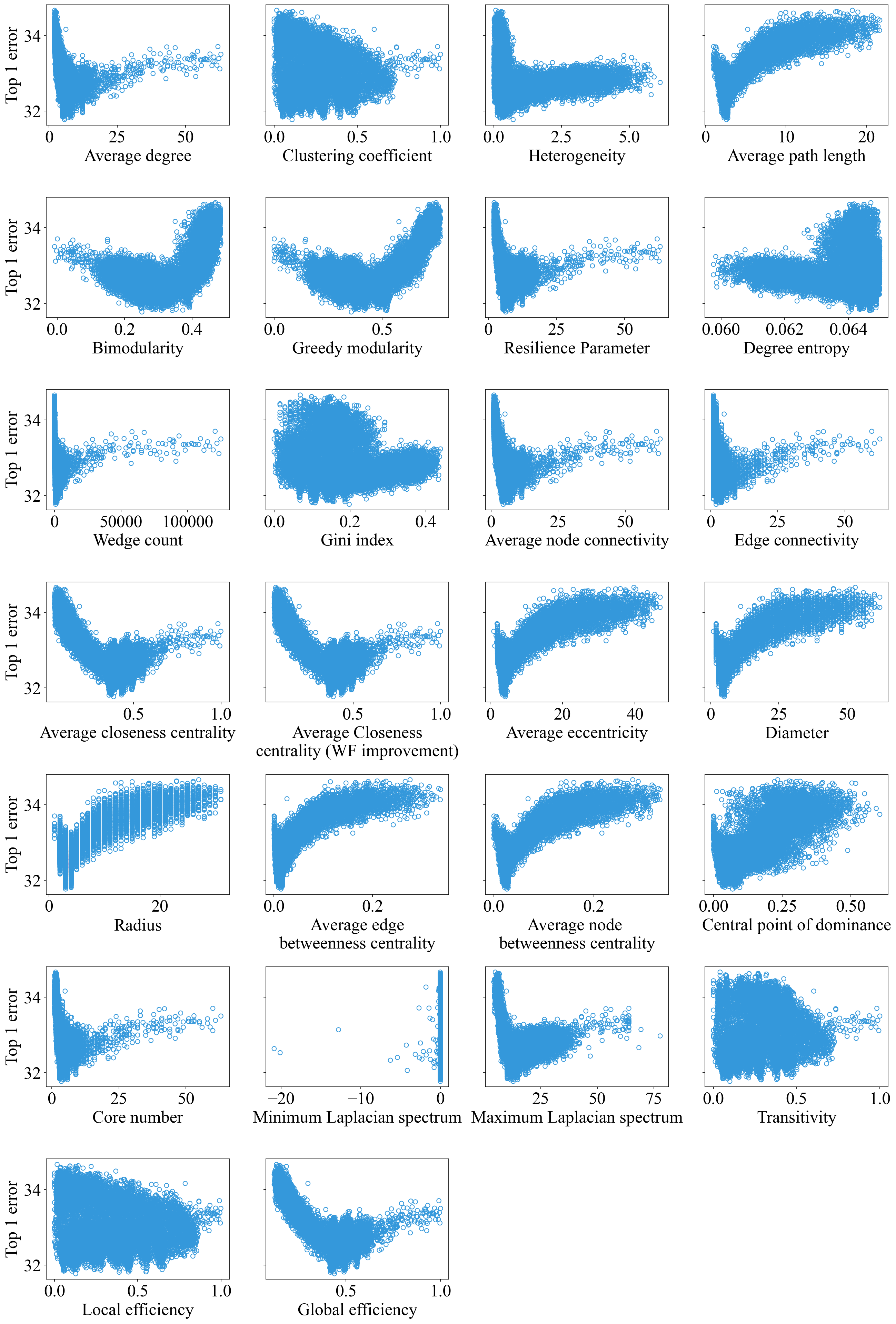
Figure 8: Top 1 errors as a function of different features. Total number of graphs is $19724$

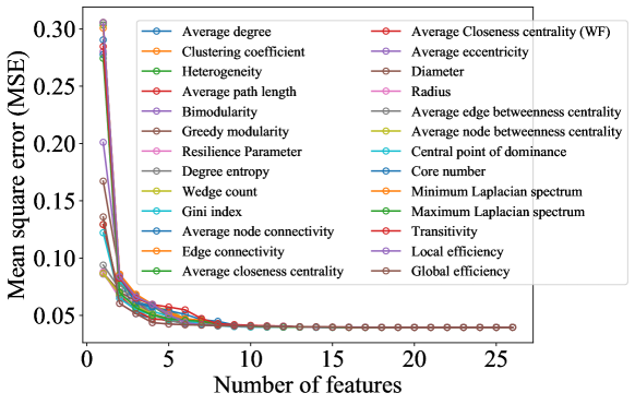
Figure 9: MSE variation with adding features

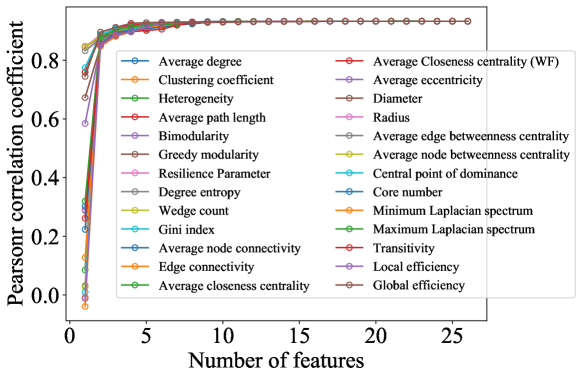
Figure 10: Pearson correlation coefficient variation with adding features

References

- Achard and Bullmore [2007] Sophie Achard and Ed Bullmore. Efficiency and cost of economical brain functional networks. PLoS computational biology, 3(2):e17, 2007.
- Albert and Barabási [2002] Réka Albert and Albert-László Barabási. Statistical mechanics of complex networks. Reviews of modern physics, 74(1):47, 2002.
- Barabási and Albert [1999] Albert-László Barabási and Réka Albert. Emergence of scaling in random networks. science, 286(5439):509–512, 1999.
- Beineke et al. [2002] Lowell W Beineke, Ortrud R Oellermann, and Raymond E Pippert. The average connectivity of a graph. Discrete mathematics, 252(1-3):31–45, 2002.
- Brandes [2001] Ulrik Brandes. A faster algorithm for betweenness centrality. Journal of mathematical sociology, 25(2):163–177, 2001.
- Brandes [2008] Ulrik Brandes. On variants of shortest-path betweenness centrality and their generic computation. Social Networks, 30(2):136–145, 2008.
- Clauset et al. [2004] Aaron Clauset, Mark EJ Newman, and Cristopher Moore. Finding community structure in very large networks. Physical review E, 70(6):066111, 2004.
- Cotter et al. [1999] Shane F Cotter, BD Rao, K Kreutz-Delgado, and J Adler. Forward sequential algorithms for best basis selection. IEE Proceedings-Vision, Image and Signal Processing, 146(5):235–244, 1999.
- Elsken et al. [2019] Thomas Elsken, Jan Hendrik Metzen, and Frank Hutter. Neural architecture search: A survey. The Journal of Machine Learning Research, 20(1):1997–2017, 2019.
- Erdos et al. [1960] Paul Erdos, Alfréd Rényi, et al. On the evolution of random graphs. Publ. Math. Inst. Hung. Acad. Sci, 5(1):17–60, 1960.
- Esfahanian [2013] Abdol-Hossein Esfahanian. Connectivity algorithms. In Topics in structural graph theory, pages 268–281. Cambridge University Press, 2013.
- Freeman [1978] Linton C Freeman. Centrality in social networks conceptual clarification. Social networks, 1(3):215–239, 1978.
- Gao et al. [2016] Jianxi Gao, Baruch Barzel, and Albert-László Barabási. Universal resilience patterns in complex networks. Nature, 530(7590):307–312, 2016.
- Goswami et al. [2018] Swati Goswami, CA Murthy, and Asit K Das. Sparsity measure of a network graph: Gini index. Information Sciences, 462:16–39, 2018.
- Gupta et al. [2016] Rishi Gupta, Tim Roughgarden, and Comandur Seshadhri. Decompositions of triangle-dense graphs. SIAM Journal on Computing, 45(2):197–215, 2016.
- Hage and Harary [1995] Per Hage and Frank Harary. Eccentricity and centrality in networks. Social networks, 17(1):57–63, 1995.
- Harary [1962] Frank Harary. The maximum connectivity of a graph. Proceedings of the National Academy of Sciences of the United States of America, 48(7):1142, 1962.
- He et al. [2016] Kaiming He, Xiangyu Zhang, Shaoqing Ren, and Jian Sun. Deep residual learning for image recognition. In Proceedings of the IEEE conference on computer vision and pattern recognition, pages 770–778, 2016.
- Hinton et al. [2012] Geoffrey Hinton, Li Deng, Dong Yu, George E Dahl, Abdel-rahman Mohamed, Navdeep Jaitly, Andrew Senior, Vincent Vanhoucke, Patrick Nguyen, Tara N Sainath, et al. Deep neural networks for acoustic modeling in speech recognition: The shared views of four research groups. IEEE Signal processing magazine, 29(6):82–97, 2012.
- Ioffe and Szegedy [2015] Sergey Ioffe and Christian Szegedy. Batch normalization: Accelerating deep network training by reducing internal covariate shift. In International conference on machine learning, pages 448–456. PMLR, 2015.
- Ji et al. [2021] Yuliang Ji, Ru Huang, Jie Chen, and Yuanzhe Xi. Generating a doppelganger graph: Resembling but distinct. arXiv preprint arXiv:2101.09593, 2021.
- Krizhevsky et al. [2009] Alex Krizhevsky, Geoffrey Hinton, et al. Learning multiple layers of features from tiny images. Citeseer, 2009.
- Krizhevsky et al. [2012] Alex Krizhevsky, Ilya Sutskever, and Geoffrey E Hinton. Imagenet classification with deep convolutional neural networks. Advances in neural information processing systems, 25:1097–1105, 2012.
- Latora and Marchiori [2001] Vito Latora and Massimo Marchiori. Efficient behavior of small-world networks. Physical review letters, 87(19):198701, 2001.
- Loshchilov and Hutter [2016] Ilya Loshchilov and Frank Hutter. Sgdr: Stochastic gradient descent with warm restarts. arXiv preprint arXiv:1608.03983, 2016.
- Luce and Perry [1949] R Duncan Luce and Albert D Perry. A method of matrix analysis of group structure. Psychometrika, 14(2):95–116, 1949.
- Marcano-Cedeño et al. [2010] Alexis Marcano-Cedeño, J Quintanilla-Domínguez, MG Cortina-Januchs, and Diego Andina. Feature selection using sequential forward selection and classification applying artificial metaplasticity neural network. In IECON 2010-36th annual conference on IEEE industrial electronics society, pages 2845–2850. IEEE, 2010.
- Nesterov [1983] Yurii E Nesterov. A method for solving the convex programming problem with convergence rate o (1/k^ 2). In Dokl. akad. nauk Sssr, volume 269, pages 543–547, 1983.
- Newman and Girvan [2004] Mark EJ Newman and Michelle Girvan. Finding and evaluating community structure in networks. Physical review E, 69(2):026113, 2004.
- Prettejohn et al. [2011] Brenton J Prettejohn, Matthew J Berryman, and Mark D McDonnell. Methods for generating complex networks with selected structural properties for simulations: a review and tutorial for neuroscientists. Frontiers in computational neuroscience, 5:11, 2011.
- Real et al. [2019] Esteban Real, Alok Aggarwal, Yanping Huang, and Quoc V Le. Regularized evolution for image classifier architecture search. In Proceedings of the aaai conference on artificial intelligence, volume 33, pages 4780–4789, 2019.
- Ru et al. [2020] Binxin Ru, Pedro Esperanca, and Fabio Carlucci. Neural architecture generator optimization. arXiv preprint arXiv:2004.01395, 2020.
- Simonyan and Zisserman [2014] Karen Simonyan and Andrew Zisserman. Very deep convolutional networks for large-scale image recognition. arXiv preprint arXiv:1409.1556, 2014.
- Sutskever et al. [2013] Ilya Sutskever, James Martens, George Dahl, and Geoffrey Hinton. On the importance of initialization and momentum in deep learning. In International conference on machine learning, pages 1139–1147. PMLR, 2013.
- Ververidis and Kotropoulos [2005] Dimitrios Ververidis and Constantine Kotropoulos. Sequential forward feature selection with low computational cost. In 2005 13th European Signal Processing Conference, pages 1–4. IEEE, 2005.
- Wasserman et al. [1994] Stanley Wasserman, Katherine Faust, et al. Social network analysis: Methods and applications. Cambridge university press, 1994.
- Watts and Strogatz [1998] Duncan J Watts and Steven H Strogatz. Collective dynamics of ‘small-world’networks. nature, 393(6684):440–442, 1998.
- Wu et al. [2016] Yonghui Wu, Mike Schuster, Zhifeng Chen, Quoc V Le, Mohammad Norouzi, Wolfgang Macherey, Maxim Krikun, Yuan Cao, Qin Gao, Klaus Macherey, et al. Google’s neural machine translation system: Bridging the gap between human and machine translation. arXiv preprint arXiv:1609.08144, 2016.
- You et al. [2020] Jiaxuan You, Jure Leskovec, Kaiming He, and Saining Xie. Graph structure of neural networks. In International Conference on Machine Learning, pages 10881–10891. PMLR, 2020.
- Zoph et al. [2018] Barret Zoph, Vijay Vasudevan, Jonathon Shlens, and Quoc V Le. Learning transferable architectures for scalable image recognition. In Proceedings of the IEEE conference on computer vision and pattern recognition, pages 8697–8710, 2018.