Metallicity in Quasar Broad Line Regions at Redshift $\sim 6$

Abstract

Broad line regions (BLRs) in high-redshift quasars provide crucial information of chemical enrichment in the early universe. Here we present a study of BLR metallicities in 33 quasars at redshift $5.7<z<6.4$. Using the near-IR spectra of the quasars obtained from the Gemini telescope, we measure their rest-frame UV emission line flux and calculate flux ratios. We then estimate BLR metallicities with empirical calibrations based on photoionization models. The inferred median metallicity of our sample is a few times the solar value, indicating that the BLR gas had been highly metal-enriched at $z\sim 6$. We compare our sample with a low-redshift quasar sample with similar luminosities and find no evidence of redshift evolution in quasar BLR metallicities. This is consistent with previous studies. The Fe ii$/$Mg ii flux ratio, a proxy for the Fe$/\alpha$ element abundance ratio, shows no redshift evolution as well, further supporting rapid nuclear star formation at $z\sim 6$. We also find that the black hole mass-BLR metallicity relation at $z\sim 6$ is consistent with the relation measured at $2<z<5$, suggesting that our results are not biased by a selection effect due to this relation.

1 Introduction

The evolution of metallicity across cosmic time contains crucial information about the star formation history and galaxy evolution. Studies of metallicity in different environments, including star-forming galaxies ($0<z<3.5$) (e.g., Tremonti et al., 2004; Maiolino et al., 2008; Mannucci et al., 2009; Zahid et al., 2014; Bian et al., 2017), Damped Lyman-$\alpha$ systems (DLAs) ($0<z<5$) (e.g., Ledoux et al., 2006; Møller et al., 2013; Prochaska et al., 2013; Rafelski et al., 2014; Bañados et al., 2019), Ly $\alpha$ emitters ($0<z<3$) (e.g., Nakajima et al., 2012, 2013; Guo et al., 2020), and quasars (up to $z\sim 7$) (e.g., Dietrich et al., 2003b; Nagao et al., 2006; Jiang et al., 2007; De Rosa et al., 2011; Xu et al., 2018; Onoue et al., 2020), have been carried out in the past two decades.

To measure metallicity in the early universe ($z\gtrsim 5.7$) and explore the reionization epoch, luminous Active Galactic Nuclei (AGNs), i.e., quasars, are among the most valuable probes given their high luminosity. In recent years, significant progress has been made in discovering high-redshift quasars (e.g., Fan et al., 2006; Willott et al., 2007, 2010; Mortlock et al., 2011; Jiang et al., 2016; Bañados et al., 2016, 2018; Matsuoka et al., 2018b, 2019; Reed et al., 2019; Yang et al., 2019, 2020; Wang et al., 2021). Near-infrared (NIR) spectroscopy of these earliest quasars reveals that the black holes (BHs) are already massive ($10^{9}\sim 10^{10}{\rm M}_{\odot}$) (Jiang et al., 2007; Kurk et al., 2007; Wu et al., 2015; Shen et al., 2019a). Studies of the BLR metallicities in these high-redshift quasars found no evidence of strong evolution compared with their low-redshift counterparts (Hamann & Ferland, 1993; Barth et al., 2003; Dietrich et al., 2003a, b, c; Nagao et al., 2006; Kurk et al., 2007; Jiang et al., 2007; Juarez et al., 2009; De Rosa et al., 2011, 2014; Mazzucchelli et al., 2017; Xu et al., 2018; Shen et al., 2019a; Shin et al., 2019; Tang et al., 2019; Schindler et al., 2020; Onoue et al., 2020).

Measurement of quasar BLR metallicities mainly relies on the rest-frame UV broad emission lines. Photoionization calculations suggest that UV line flux ratios, including (Si IV+O IV])$/$C IV, (C III]+Si III])$/$C IV, Al III$/$C IV, N v$/$C IV, He ii$/$C IV, and N v$/$He ii can be used to infer metallicities (Hamann et al., 2002; Nagao et al., 2006). Nagao et al. (2006) used a large quasar sample from the SDSS, and measured different diagnostic flux ratios from the composite spectra in each redshift and absolute B magnitude ($M_{B}$) bin. No significant redshift evolution was found in the redshift range of $2<z<4.5$. By comparing the observed line flux ratios with their photoionization calculations, the BLR metallicities are estimated to be ${\rm Z}\sim 5{\rm Z}_{\odot}$ (solar metallicity). Jiang et al. (2007) performed a similar analysis for six quasars at $z\sim 6$, and the BLR metallicity is found to be consistent with those in low-redshift quasars (${\rm Z}\sim 4{\rm Z}_{\odot}$).

On the other hand, a significant positive correlation between BLR metallicity and quasar luminosity is found in Nagao et al. (2006). As suggested by the paper, the more fundamental relation is the mass-metallicity relation (MZR) in AGNs (Matsuoka et al., 2011; Xu et al., 2018), i.e., more massive BHs are accompanied by BLRs with higher metallicities. The origin of the MZR relation is unclear, but is likely connected to the galaxy MZR via the BH mass-host galaxy relation (Matsuoka et al., 2011, 2018a; Dors et al., 2015).

Another critical finding in quasar metallicity studies is the non-redshift evolution of Fe ii$/$Mg ii, which is the first-order proxy of the Fe$/\alpha$ element abundance ratio. This ratio acts like a clock of the star formation history, since the Fe element is mainly ejected by Type Ia supernovae (SN Ia), which is delayed by $\sim$1 Gyr relative to $\alpha$ elements that are mainly produced by core collapsed supernovae (Type II and Type Ib/Ic supernovae). Many studies measured the Fe ii$/$Mg ii ratio (Dietrich et al., 2003b; Kurk et al., 2007; Jiang et al., 2007; De Rosa et al., 2011, 2014; Mazzucchelli et al., 2017; Shin et al., 2019; Schindler et al., 2020; Onoue et al., 2020; Yang et al., 2021), and no redshift evolution was found up to $z\sim 7$. This result suggests a rapid star formation in the nucleus at earlier epochs to produce the observed iron abundance in $z\sim 6$ quasar BLRs.

Shen et al. (2019a) conducted a large spectroscopic survey of 50 $z\geq 5.7$ quasars using Gemini GNIRS with a simultaneous coverage in NIR. This sample is a valuable data set to study the physical properties of high-redshift quasars as well as intervening absorption systems that trace the intergalactic medium (IGM) and the circum-galactic medium (CGM) (Zou et al., 2021). Shen et al. (2019a) performed an initial analysis of the sample, focusing on BH masses, emission line shifts, and other general spectral properties. They found that the median composite spectrum of $z\sim 6$ quasars is similar to that generated from a luminosity-matched control sample at lower redshifts.

In this paper, we perform a quantitative analysis to measure quasar BLR metallicity of the GNIRS sample and study its redshift evolution. Although similar analyses have been performed in the past, our GNIRS sample has the advantages of better sample statistics, and a more complete coverage of multiple UV broad lines to measure the BLR metallicity with different indicators. The paper is organized as follows. We describe the observations and sample selection in §2. The detailed spectral decomposition is presented in §3. In §4 we study the redshift evolution of BLR metallicities and the Fe ii$/$Mg ii ratio. We discuss the implications of our results in §5 and summarize in §6. Throughout this paper, we adopt a flat lambda cold dark matter cosmology with $\Omega_{0}=1-\Omega_{\Lambda}=0.3$ and ${\rm H}_{0}=70\;{\rm km}/{\rm s}\;{\rm Mpc}^{-1}$.

2 Sample and Data

We use the high-redshift quasars from Shen et al. (2019a) as our parent sample. This parent sample is collected from identified quasars at $z\geq 5.7$ in the literature. 51 quasars were observed during the 15B-17A semesters using GNIRS on Gemini-North. One object was removed from the sample because of poor observing conditions, and the final parent sample contains 50 quasars. The properties of the parent sample, including coordinates, $J$ band photometry, and the discovery references, are summarized in Table 1 of Shen et al. (2019a). The parent sample is not a complete flux-limited sample at $z\geq 5.7$, but it includes quasars with diverse properties in terms of luminosity and spectral properties.

The GNIRS observations were conducted in the cross-dispersion mode using the short blue camera with a slit width of $0$$\farcs$$675$. The wavelength coverage of the spectroscopy is 0.85-2.5$~{}\mu$m, with a spectral resolution of $R\sim 650$. The exposure time varies from 30 minutes to 5 hours depending on the brightness of the target. The obtained signal-to-noise ratio (S/N) is 5 per pixel averaged over $H$ band.

The GNIRS data were reduced using a custom pipeline based on two existing pipelines for GNIRS: the PyRAF-based XDGNIRS (Mason et al., 2015) and the IDL-based XIDL package. The spectrum is scaled to the available $J$ band magnitude for absolute flux calibration. Detailed data reduction is described in Section 2.1 of Shen et al. (2019a).

Starting from this parent sample, we perform an initial spectral analysis as described in §3. We found that some quasars have low S/N, peculiar continuum shapes likely caused by reduction or intrinsic reddening, or significantly affected by strong telluric line residuals. To robustly measure C IV based metallicity and Fe ii$/$Mg ii, we exclude objects for which neither C IV nor Mg ii can be reasonably fitted (see §3). The final sample for our study contains 33 quasars.

3 Spectral analysis

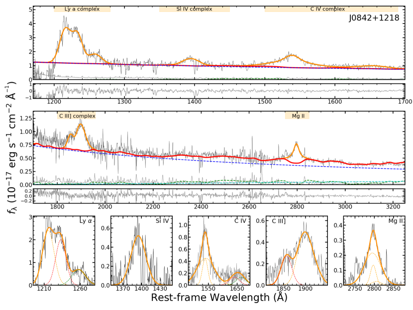
Figure 1: An example of our spectral analysis. The upper panels present the global continuum fitting results and the residuals in two spectral regions. The black and grey lines represent the original flux and error spectrum, respectively. The red and orange solid lines are the pseudo-continuum and emission line models, respectively. Different line complexes are labeled on the top and the light orange shaded areas denote the wavelength ranges to fit each complex. The bottom-row panels display the fits to the pseudo-continuum-subtracted line profiles in different line complexes, Ly $\alpha$, Si IV, C IV, C III], and Mg ii, from left to right. The orange, red and green dashed Gaussians represent the main components in each complex, decomposed components used to indicate metallicity, and those not used in metallicity estimation but included in the fitting, respectively. The complete figure set for 33 objects are available in the online journal.

We fit the NIR spectra with multi-component models, following earlier work (e.g., Shen et al., 2011, 2019b; Wang et al., 2020). In the fitting procedure, we correct the effects of narrow absorption lines with iterative sigma clipping. We visually check the initial fitting results, and interactively add additional pixel masks to exclude broad absorption features in the fits on an object-by-object basis. We exclude individual line complex regions if, e.g., the underlying continuum has peculiar shapes and/or the absorption features are too broad to be fully masked. In addition, we mask the spectral regions where the spectrum is heavily affected by telluric absorption. These telluric regions are generally $\lambda_{\rm obs}=13400-14500$ Å and $\lambda_{\rm obs}=17800-19000$ Å, but are slightly adjusted based on the initial fitting results.

After the initial fits, we perform the final fits in the rest-frame of the quasar using the systemic redshifts, $z_{\rm sys}$, provided in Shen et al. (2019a). An example of our spectral modeling (J0842+1218) is shown in Figure 1. The complete figure set of our fits is available in the online journal.

During the spectral modeling, we first fit a pseudo-continuum model to several emission-line-free windows, and then fit each line complex after subtracting the pseudo-continuum model. These line complexes are Ly $\alpha$$+$N v, Si IV$+$O IV], C IV$+$He ii$+$[O iii], C III]$+$Si III]$+$Al III, and Mg ii complex. The pseudo-continuum model is described in §3.1, and the emission-line models are described in §3.2. §3.3 summarizes our spectral measurements and derived physical quantities, including BH masses, bolometric luminosities, and Eddington ratios.

3.1 The continuum model

We fit a global continuum in order to measure different line flux ratios consistently across the spectrum. We choose the commonly used continuum windows in the rest-frame UV, which consist of several emission-line free wavelength regions, including $\lambda_{\rm rest}$ = $1345-1350$, $1445-1450$, $1700-1705$. $2150-2400$, $2480-2675$, and $2900-3450$ Å. The continuum models used in our fits consist of a power law component $F_{\rm PL}$, a Balmer continuum component $F_{\rm BC}$, and a broad Fe ii emission component $F_{\rm Fe}$. Different from Shen et al. (2019a), we do not add an additional polynomial component to account for the peculiar continuum shapes in some objects caused by intrinsic reddening or flux calibration issues. This component would introduce additional systematic uncertainties to the Fe ii$/$Mg ii measurement. Instead, we exclude the object from our sample if we cannot fit the original spectrum well by only including the model components described above, as judged by visual inspection.

The power law model $F_{\rm PL}$ is normalized at 3000 Å, and described by:

$$F_{\rm PL}(\lambda;\;\alpha,\beta)=\alpha\left(\frac{\lambda}{3000}\right)^{\beta}\ ,$$ (1)

where $\alpha$ and $\beta$ are the flux scaling factor and the power-law slope, respectively.

The Balmer continuum model $F_{\rm BC}$ is described by the following equation:

$$F_{\rm BC}=\gamma\,B_{\lambda}(\lambda,T_{e})\;(1-e^{-\tau_{\lambda}})\;;\lambda\leq\lambda_{\rm BL},$$ (2)

where $\gamma$ is the flux scaling factor and $B_{\lambda}(\lambda,T_{e})$ is the Plank function at temperature $T_{e}$. $\lambda_{\rm BL}=3646$ Å is the wavelength of Balmer limit. $\tau_{\lambda}=\tau_{\rm BL}(\lambda/\lambda_{\rm BL})^{3}$ is the optical depth normalized by the value of Balmer limit. The normalization of the Balmer continuum is commonly determined at $\lambda=3675$ Å, where there is no obvious contamination from iron emission. However, because of the limited spectral coverage of our spectrum, $F_{\rm BC}$ and $F_{\rm PL}$ are highly degenerated in our fits. Thus, we follow previous studies (Dietrich et al., 2003b; Kurk et al., 2007; De Rosa et al., 2011; Mazzucchelli et al., 2017; Shin et al., 2019; Schindler et al., 2020; Onoue et al., 2020) and set the flux density of Balmer continuum component to be 30% of that of power law component at the Balmer limit, as described by the following equation:

$$F_{\rm BC}(\lambda=3646)=0.3\times F_{\rm PL}(\lambda=3646).$$ (3)

The Fe ii pseudo-continuum $F_{\rm Fe}$ is fitted with an empirical template $F_{\rm Template}$. The free parameters include the flux scaling factor, the width of the broadening kernel, and the wavelength shift, as described by:

$$F_{\rm Fe}=\zeta F_{\rm Template}|_{\lambda\times(1+\delta)}\circledast G(\lambda,\sigma),$$ (4)

where $\zeta$ is the flux scaling factor, $G(\lambda,\sigma)$ is a Gaussian broadening kernel with a kernel width $\sigma$, and $\delta$ is the wavelength shift parameter.

One of the commonly used Fe ii templates in the rest-frame UV wavelength range was provided by Vestergaard & Wilkes (2001), hereafter the VW01 template. The VW01 template was constructed based on the high S/N HST spectra of a narrow-line Seyfert 1 AGN, I Zwicky 1. In the wavelength region beneath Mg ii ($2780-2830$ Å), the flux of the VW01 template is set to be zero. Tsuzuki et al. (2006) presented a Fe ii template (hereafter the T06 template) that uses information from photoionization calculations (Ferland et al., 1998). The two templates are generally consistent with each other. However, Woo et al. (2018) compared the fitting results based on these two templates and found that the Mg ii (Fe ii) flux using the VW01 template is systematically higher (lower) compared to the measurements based on the T06 template. This will introduce a systematic bias when we compare Fe ii$/$Mg ii ratios from the literature using different Fe ii templates.

In this work, we adopt the VW01 template, since many empirical scaling relations and BH mass estimators are based on this template. We compare with the fitting results using the T06 template in the Appendix. Note that the T06 template only covers the wavelength region of $\lambda\geq 2200$ Å. In the $\lambda<2200$ Å region, the T06 template is augmented by the VW01 template. Therefore, the choice of the Fe ii template will only affect the Fe ii$/$Mg ii ratio, but have little effect on other UV line flux ratios. This is also supported by Onoue et al. (2020) (see their Table 3).

3.2 Emission line models

We focus on main metallicity diagnostic lines including C IV, He ii, Si IV, N v, C III], Al III, and Mg ii. Many of them are blended with other emission lines, e.g., N v $\lambda 1240$ with Ly $\alpha$, [S II]  $\lambda 1256$, and [Si II]  $\lambda 1263$, Si IV $\lambda\lambda 1394,1403$ with O IV] $\lambda 1402$, and C III] $\lambda\lambda 1907,1909$ with Si III] $\lambda 1872$. Therefore, we attempt to decompose these lines in individual line complexes. Table 1 summarizes all lines included in our spectral analysis and the fitting ranges for each line complex.

We use multiple Gaussians to fit the line profile in each complex. Some earlier works also used a broken power-law model (e.g., Nagao et al., 2006; Matsuoka et al., 2011; Xu et al., 2018) to describe the line profile. They divide lines into high and low ionization line groups and assume all lines in the same group have the same power-law indices and line shifts. This can be over-simplified, e.g., C III] and Mg ii may have different line shifts (Shen et al., 2016). Nagao et al. (2006) also found that fitting results using multiple Gaussians are as good as those from the broken power-law model. Table 1 shows the number of Gaussians used in our fits. We generally do not include UV narrow line components given the spectral quality, unless they are relatively strong and obvious, e.g., Mg ii lines for some quasars. The inclusion of narrow lines in such cases is important, since it affects the measurement of the broad-line full-width-at-half-maximum (FWHM), which is used in the BH mass estimation.

Table 1: Fitting parameters

Line complex	Fitting range	Line	${{\rm n}_{\rm gauss}}^{a}$
Mg ii	$2750-2850$	Mg ii	3B$+$2N
C III]	$1800-1960$	C III]$+$Si III]	2B
		Al III	1B
C IV	$1500-1690$	C IV	3B
		He ii	1B
		O IV]	1B
Si IV	$1350-1450$	Si IV$+$O IV]	2B
Ly $\alpha$	$1200-1280$	Ly $\alpha$	2B+1N
		N v	1B
		[S II]$+$[Si II]	1B
Note. a. In the last column, B and N refer to the Gaussians used for the broad- and narrow-line components, respectively.

Apart from being blended with Fe ii, the main difficulty in fitting Mg ii is the contamination from telluric absorptions. For the typical redshift of our sample ($z\sim 6$), Mg ii shifts to 19,600 Å in the observed frame. The blue wing of Mg ii, or even most of the line profile, can be affected by the telluric absorption. Therefore, we adjust the blue side boundary when necessary for individual objects. We exclude some objects whose Mg ii lines are severely affected by the telluric absorption.

C III] can also be affected by telluric absorption. However, we find that the telluric absorption within $13,400<\lambda_{\rm obs}<14,500$ Å usually only affects a very small portion of the C III] profile, and many of the affected objects are already excluded from the continuum fitting step. Only one C III] fit suffered from severe telluric effects and was excluded from our analysis. In the fitting of C III]  the main problem is that it is heavily blended with Si III]. In our emission-line fitting, we use the total flux of the C III]$+$Si III] complex, same as in Jiang et al. (2007). We do not include narrow components for the C III] complex.

Al III is relatively weak compared to C III] $+$ Si III]. It also blends with C III] $+$ Si III], but can be easily deblended in most of our objects. We exclude Al III flux measurements with large uncertainties (more than 30% of the line flux) or with broader line widths compared to the C III] $+$ Si III] complex. These are due to low S/Ns.

It is sometimes difficult to decompose He ii $\lambda 1640$ and [O iii] $\lambda 1663$ because of a $\lambda 1600$ feature (Nagao et al., 2006) that is likely due to imperfect subtraction of Fe ii and Fe iii from the empirical template. In our work, we set the center of [O iii] and He ii within $[1656,1663]$ Å and $[1620,1640]$ Å, respectively. As for Al III, We exclude the flux measurements with large uncertainties.

Si IV is heavily blended with O IV]. We treat Si IV and O IV] as one integrated component and use two broad Gaussians to fit. The Si IV line complexes are often weak compared to the flux uncertainties, and suffer from absorption lines. We exclude Si IV measurements with large uncertainties.

Our N v measurements can be affected by the absorption of N v or Ly $\alpha$. We exclude objects that are severely affected by absorption. For the remaining objects, we mask the affected wavelength pixels and fit the line profile with a single Gaussian. In general, our masks provide reasonable fits (see the full figure set of Figure 1 in the online version).

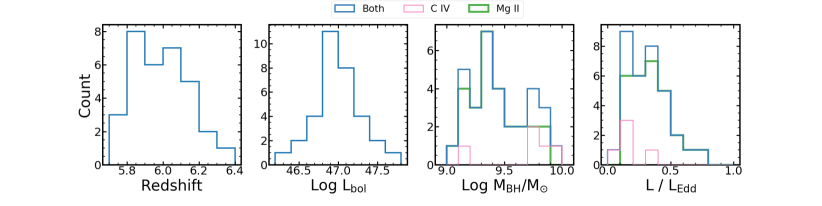
Figure 2: Left to right: the distributions of redshift, bolometric luminosity ${\rm Log}\;{L}_{\rm bol}$, BH mass ${\rm Log}\;{M}_{\rm BH}/{M}_{\rm\odot}$, and Eddington ratio ${L}/{L}_{\rm Edd}$. In the third and fourth panels, the green and pink histograms indicate the the sub-sample where the quantity is derived using Mg ii and C IV, respectively, while the blue denotes the sum of the two.

3.3 Spectral measurements and derived physical properties

All spectral quantities are measured from the best-fit models. We measure the flux density and monochromatic luminosity at the rest-frame $1350$ and $3000$ Å. We also measure the FWHMs of broad Mg ii and C IV to estimate BH masses. The Fe ii flux is computed by integrating the best-fit Fe ii model over the rest-frame wavelength range $2200<\lambda<3090$ Å (De Rosa et al., 2011; Shen et al., 2011). For broad emission-line flux, we calculate the sum of the multiple Gaussians integrated over the full line profile.

We estimate the uncertainties of our measurements using the Monte Carlo method. We generate 50 mock spectra for each object by adding Gaussian random fluxes at each wavelength pixel to perturb the original spectrum. The Gaussian width is set to the flux uncertainties at each wavelength pixel. The same fitting procedure is applied to all mock spectra to derive the distribution of a given spectral quality. The final uncertainties of spectral measurements are the semi-amplitude of the range enclosing the 16th to 84th percentiles of the distribution.

We present the estimates of quasar BH mass $M_{\rm BH}$, bolometric luminosity $L_{\rm bol}$, and Eddington ratio $L/L_{\rm Edd}$. The BH masses are measured mainly based on the broad Mg ii, which are shown to correlate well with those estimated from broad Balmer lines (Wang et al., 2009; Shen et al., 2011). For four objects in our sample that do not have robust Mg ii measurements, we use the broad C IV line (Vestergaard & Peterson, 2006; Shen et al., 2011). The bolometric luminosity is estimated by $L_{\rm bol}=5.15\times\lambda L_{\lambda}$ at $\lambda=3000$ Å  (Richards et al., 2006). Uncertainties in these derived quantities are estimated from the error propagation. Table 2 lists these properties and their distributions are shown in Figure 2. Our measurements are generally consistent with those reported in Shen et al. (2019a) within uncertainties, with minor differences due to different fitting components (e.g., we added the Balmer continuum component). In particular, our $L_{3000}$ are 0.1 dex lower than those in Shen et al. (2019a), and the Mg ii FWHM is different in some objects where we included a narrow Mg ii component. Nevertheless, these minor differences do not impact our results.

=1.5in

Table 2: Quasar properties and emission line flux ratios

Name	$z_{sys}$	log $L_{\rm bol}$	log $M_{\rm BH}$	Source	$L/L_{\rm Edd}$	Si IV$/$C IV	C III]$/$C IV	Al III$/$C IV	He ii$/$C IV	N v$/$C IV	N v$/$He ii
J0002$+$2550	$5.818\pm 0.007$	$47.180\pm 0.003$	$9.36\pm 0.05$	Mg ii	$0.50\pm 0.06$	$0.50\pm 0.07$	$0.51\pm 0.02$	$0.14\pm 0.02$	…	…	…
J0008$-$0626	$5.929\pm 0.006$	$46.964\pm 0.013$	$9.19\pm 0.07$	Mg ii	$0.45\pm 0.07$	$0.47\pm 0.06$	$0.62\pm 0.05$	$0.11\pm 0.01$	…	$0.99\pm 0.21$	…
J0028$+$0457	$5.982\pm 0.001$	$46.969\pm 0.020$	$9.91\pm 0.13$	C IV	$0.09\pm 0.02$	$0.52\pm 0.07$	…	…	…	$1.06\pm 0.29$	…
J0050$+$3445	$6.251\pm 0.006$	$47.103\pm 0.007$	$9.76\pm 0.12$	Mg ii	$0.17\pm 0.04$	$0.41\pm 0.05$	…	…	$0.23\pm 0.06$	$0.77\pm 0.15$	$3.56\pm 0.15$
J0353$+$0104	$6.057\pm 0.005$	$46.975\pm 0.042$	$9.32\pm 0.17$	Mg ii	$0.35\pm 0.10$	…	…	…	…	…	…
J0810$+$5105	$5.805\pm 0.010$	$47.193\pm 0.009$	$9.29\pm 0.11$	Mg ii	$0.61\pm 0.14$	…	$0.53\pm 0.03$	$0.19\pm 0.04$	$0.30\pm 0.06$	$1.41\pm 0.26$	$4.80\pm 0.26$
J0835$+$3217	$5.902\pm 0.009$	$46.286\pm 0.006$	$8.91\pm 0.10$	Mg ii	$0.18\pm 0.04$	$0.40\pm 0.07$	$0.41\pm 0.05$	$0.11\pm 0.03$	$0.33\pm 0.09$	$0.75\pm 0.09$	$2.47\pm 0.09$
J0836$+$0054	$5.834\pm 0.007$	$47.621\pm 0.004$	$9.61\pm 0.08$	Mg ii	$0.79\pm 0.15$	$0.49\pm 0.08$	$0.59\pm 0.07$	$0.30\pm 0.13$	$0.14\pm 0.03$	$1.54\pm 0.11$	$11.93\pm 0.11$
J0840$+$5624	$5.816\pm 0.010$	$46.556\pm 0.013$	$9.17\pm 0.12$	Mg ii	$0.19\pm 0.05$	$0.39\pm 0.05$	$0.67\pm 0.06$	$0.15\pm 0.02$	$0.18\pm 0.05$	…	…
J0841$+$2905	$5.954\pm 0.005$	$46.986\pm 0.008$	$9.40\pm 0.19$	Mg ii	$0.29\pm 0.12$	$0.24\pm 0.06$	…	…	…	$1.03\pm 0.22$	…
J0842$+$1218	$6.069\pm 0.009$	$47.196\pm 0.005$	$9.52\pm 0.06$	Mg ii	$0.36\pm 0.04$	$0.36\pm 0.06$	$0.49\pm 0.03$	$0.17\pm 0.02$	$0.16\pm 0.05$	$0.85\pm 0.06$	$5.18\pm 0.06$
J1044$-$0125	$5.780\pm 0.007$	$47.311\pm 0.006$	$9.81\pm 0.10$	Mg ii	$0.24\pm 0.05$	$0.42\pm 0.03$	$0.53\pm 0.04$	$0.21\pm 0.02$	$0.18\pm 0.05$	$1.05\pm 0.08$	$5.32\pm 0.08$
J1137$+$3549	$6.009\pm 0.010$	$47.282\pm 0.008$	$9.76\pm 0.09$	Mg ii	$0.25\pm 0.05$	$0.34\pm 0.05$	$0.38\pm 0.03$	$0.13\pm 0.02$	$0.14\pm 0.04$	$0.98\pm 0.10$	$5.47\pm 0.10$
J1143$+$3808	$5.800\pm 0.010$	$46.999\pm 0.005$	$9.73\pm 0.08$	C IV	$0.14\pm 0.02$	…	$0.52\pm 0.04$	$0.07\pm 0.02$	$0.21\pm 0.06$	$1.00\pm 0.12$	$5.09\pm 0.12$
J1148$+$0702	$6.344\pm 0.006$	$47.091\pm 0.013$	$9.38\pm 0.20$	Mg ii	$0.39\pm 0.17$	$0.46\pm 0.06$	$0.46\pm 0.07$	$0.17\pm 0.03$	$0.20\pm 0.05$	$0.75\pm 0.08$	$6.04\pm 0.08$
J1148$+$5251	$6.416\pm 0.006$	$47.533\pm 0.004$	$9.82\pm 0.09$	Mg ii	$0.40\pm 0.08$	$0.31\pm 0.05$	…	…	…	…	…
J1207$+$0630	$6.028\pm 0.013$	$46.909\pm 0.011$	$9.53\pm 0.08$	Mg ii	$0.18\pm 0.03$	$0.46\pm 0.06$	$0.56\pm 0.05$	$0.20\pm 0.05$	…	…	…
J1243$+$2529	$5.842\pm 0.006$	$47.060\pm 0.004$	$9.84\pm 0.05$	C IV	$0.13\pm 0.01$	$0.25\pm 0.09$	$0.37\pm 0.02$	$0.09\pm 0.02$	$0.16\pm 0.04$	…	…
J1250$+$3130	$6.138\pm 0.005$	$46.988\pm 0.005$	$9.13\pm 0.06$	Mg ii	$0.56\pm 0.07$	$0.36\pm 0.02$	$0.39\pm 0.03$	$0.05\pm 0.03$	$0.13\pm 0.03$	$0.99\pm 0.07$	$7.91\pm 0.07$
J1257$+$6349	$5.992\pm 0.010$	$46.739\pm 0.013$	$9.43\pm 0.10$	Mg ii	$0.16\pm 0.03$	…	…	…	…	…	…
J1429$+$5447	$6.119\pm 0.008$	$46.831\pm 0.005$	$9.18\pm 0.18$	Mg ii	$0.34\pm 0.14$	…	…	…	…	…	…
J1436$+$5007	$5.809\pm 0.010$	$47.044\pm 0.012$	$9.30\pm 0.18$	Mg ii	$0.42\pm 0.16$	…	$0.68\pm 0.15$	…	…	$1.09\pm 0.17$	…
J1545$+$6028	$5.794\pm 0.007$	$46.532\pm 0.013$	$9.20\pm 0.05$	C IV	$0.17\pm 0.02$	$0.22\pm 0.04$	$0.39\pm 0.02$	$0.07\pm 0.02$	$0.09\pm 0.01$	$1.03\pm 0.10$	$11.60\pm 0.10$
J1602$+$4228	$6.083\pm 0.005$	$47.210\pm 0.009$	$9.42\pm 0.08$	Mg ii	$0.47\pm 0.07$	$0.33\pm 0.05$	$0.59\pm 0.03$	$0.15\pm 0.01$	$0.19\pm 0.06$	…	…
J1609$+$3041	$6.146\pm 0.006$	$46.645\pm 0.009$	$9.44\pm 0.10$	Mg ii	$0.12\pm 0.02$	$0.45\pm 0.09$	…	…	$0.16\pm 0.04$	$0.92\pm 0.08$	$7.89\pm 0.08$
J1623$+$3112	$6.254\pm 0.006$	$46.975\pm 0.003$	$9.32\pm 0.15$	Mg ii	$0.35\pm 0.12$	$0.33\pm 0.09$	$0.46\pm 0.07$	$0.06\pm 0.02$	$0.12\pm 0.05$	$0.91\pm 0.09$	$5.89\pm 0.09$
J1630$+$4012	$6.066\pm 0.007$	$46.760\pm 0.007$	$9.27\pm 0.10$	Mg ii	$0.24\pm 0.05$	$0.17\pm 0.03$	$0.27\pm 0.02$	$0.06\pm 0.02$	…	$0.83\pm 0.13$	…
J2310$+$1855	$5.956\pm 0.011$	$47.464\pm 0.005$	$9.66\pm 0.15$	Mg ii	$0.49\pm 0.16$	$0.46\pm 0.05$	…	…	…	…	…
P000$+$26	$5.733\pm 0.007$	$47.333\pm 0.034$	$9.70\pm 0.09$	C IV	$0.33\pm 0.04$	…	$0.55\pm 0.04$	$0.06\pm 0.03$	$0.16\pm 0.03$	…	…
P060$+$24	$6.170\pm 0.006$	$47.057\pm 0.013$	$9.32\pm 0.03$	Mg ii	$0.42\pm 0.02$	$0.47\pm 0.07$	$0.54\pm 0.09$	$0.12\pm 0.02$	$0.17\pm 0.05$	$1.10\pm 0.19$	$6.51\pm 0.19$
P210$+$27	$6.166\pm 0.007$	$46.910\pm 0.017$	$9.33\pm 0.11$	Mg ii	$0.29\pm 0.06$	$0.35\pm 0.09$	…	$0.11\pm 0.03$	$0.13\pm 0.03$	…	…
P228$+$21	$5.893\pm 0.015$	$46.605\pm 0.007$	$9.07\pm 0.06$	Mg ii	$0.26\pm 0.03$	…	$0.57\pm 0.06$	…	…	…	…
P333$+$26	$6.027\pm 0.007$	$46.839\pm 0.017$	$9.24\pm 0.10$	Mg ii	$0.30\pm 0.05$	…	$0.57\pm 0.13$	$0.17\pm 0.05$	$0.18\pm 0.06$	…	…
Median	$5.992\pm 0.172$	$46.990\pm 0.289$	$9.36\pm 0.25$	All	$0.30\pm 0.16$	$0.39^{+0.07}_{-0.10}$	$0.53^{+0.06}_{-0.13}$	$0.12^{+0.06}_{-0.06}$	$0.17^{+0.04}_{-0.03}$	$0.99^{+0.10}_{-0.17}$	$5.67^{+2.23}_{-0.86}$
Composite	…	…	…	…	…	$0.33\pm 0.06$	$0.48\pm 0.02$	$0.13\pm 0.02$	$0.15\pm 0.02$	$0.95\pm 0.15$	$5.70\pm 0.65$

4 Results

4.1 UV line flux ratios and metallicity

Table 2 summarizes the results of the main diagnostic line flux ratios for metallicity estimates, including Si IV$/$C IV, C III]$/$C IV, Al III$/$C IV, N v$/$C IV, He ii$/$C IV, and N v$/$He ii. In this section we explore the dependence of these flux ratios on redshift, and estimate BLR metallicities using empirical relations calibrated by photoionization models. For simplicity, we use the name of the main line in each line complex to refer to the whole line complex, e.g., Si IV for Si IV$+$O IV]and C III] for C III]$+$Si III].

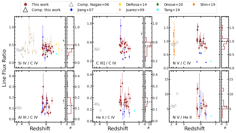
Figure 3: Different line flux ratios (labeled at the lower left corner) as a function of redshift. Different samples are plotted with different colors, as shown in the top legend. The points represent individual measurements, while the triangles are the values measured from composite spectra. The x-axis is scaled for display purpose. For each panel of flux ratios, we plot the histogram of the line flux ratio distribution for our sample on the right sidebar. The black dashed horizontal lines indicate the median values of our sample.

Table 3: Sample Summary

Sample	Redshift	Median $M_{B}$	$M_{B}$ range	Size	Metallicity indicatora
This work	$5.7<z<6.4$	$-27.2$	$-26.4\sim-28.5$	30b	Si IV$/$C IV, C III]$/$C IV, Al III$/$C IV
					He ii$/$C IV, N v$/$C IV, N v$/$He ii
Other high redshift sample
Onoue et al. (2020)	$7.5$	$-27.2$	…	1	Si IV$/$C IV, C III]$/$C IV, Al III$/$C IV
De Rosa et al. (2014)	$6.6<z<7.1$	$-26.4$	$-26.1\sim-27.2$	4	Si IV$/$C IV
Tang et al. (2019)	6.6	$-26.1$	…	1	Si IV$/$C IV, He ii$/$C IV, N v$/$C IV, N v$/$He ii
Jiang et al. (2007)	$5.8<z<6.3$	$-27.6$	$-27.2\sim-28.5$	6	Same as this paper
Juarez et al. (2009)	$4<z<6.4$	$-27.2$	$-26.2\sim-29.0$	30	Si IV$/$C IV
Lower redshift sample
Nagao et al. (2006)	$2.0<z<4.5$	…	$-26.5\sim-28.5$	2317	Same as this work
Shin et al. (2019)	$3.0<z<3.4$	$-25.9$	$-24.7\sim-28.7$	12	N v$/$C IV
Note. a. De Rosa et al. (2014) and Tang et al. (2019) fit C III]$+$Si III]$+$Al III as a single line and we do not include these measurements here. The N v$/$He ii ratio in Jiang et al. (2007) was estimated from N v$/$C IV and He ii$/$C IV. b. Three objects in our sample cannot obtain robust fit for C IV, thus cannot be used to study metallicity. They are only used in the study of Fe ii$/$Mg ii.

To study redshift evolution, we compare our sample ($5.7<z<6.5$) with earlier samples at other redshifts ($2<z<7.5$) (Nagao et al., 2006; Jiang et al., 2007; Juarez et al., 2009; De Rosa et al., 2014; Shin et al., 2019; Onoue et al., 2020). Nagao et al. (2006) studied quasar flux ratios at $2<z<4.5$ and $-29.5<{M}_{B}<-24.5$. As mentioned in the introduction, a significant correlation between metallicity and $M_{B}$ was found. Therefore, to study the redshift evolution, we need to compare samples with similar luminosities. The $M_{B}$ magnitudes of our sample are derived from $M_{1450}$ compiled from the literature (Jiang et al., 2016; Willott et al., 2010; Bañados et al., 2016), assuming a spectral index $\alpha_{\upsilon}=-0.5$ following Richards et al. (2006). Note that for our quasars, the conversion of $M_{B}$ from $M_{1450}$ is an extrapolation from the GNIRS spectrum, but the adopted power-law index is a good approximation in the range of $1450<\lambda_{\rm rest}<5000$ Å (Vanden Berk et al., 2001). The median $M_{B}$ value of our sample is $-27.2$, ranging from $-26.4$ to $-28.5$. Therefore, we select two bins from Nagao et al. (2006), $-26.5<{M}_{B}<-27.5$ and $-27.5<{M}_{B}<-28.5$, and calculated average flux ratios in $-26.5<{M}_{B}<-28.5$ in each redshift bin weighted by the number of objects in each bin. Apart from Nagao et al. (2006), other studies also provide various line flux ratios in different redshift ranges (Jiang et al., 2007; Juarez et al., 2009; Shin et al., 2019; Onoue et al., 2020). We summarize these earlier samples in Table 3.

Figure 3 displays various line ratios as a function of redshift compiled from different samples. Although the scatter is large, the median values of these line flux ratios are consistent with no redshift evolution within $2\lesssim z\lesssim 6$. These median values of our sample are summarized in Table 2. We also generate a high S/N median composite spectrum of our final sample following Shen et al. (2019a), and found consistent results in the average line flux ratios (open triangles in Fig. 3).

Our results are generally consistent with other high-redshift studies (Jiang et al., 2007; Juarez et al., 2009; De Rosa et al., 2014; Tang et al., 2019; Onoue et al., 2020). Two objects, J0836$+$0054 and J1044$-$0125, overlap with both Jiang et al. (2007) and Juarez et al. (2009). Additional five objects, J0002$+$2550, J1148$+$5251, J1602$+$4228, J1623$+$3112, and J1630$+$4012, overlap with Juarez et al. (2009). The Si IV$/$C IV ratios of these objects are consistent ($\leq 1\sigma$) among different studies. For N v$/$C IV in the two objects overlapping with Jiang et al. (2007), one object is consistent within 1$\sigma$ uncertainty and the other one shows a difference. It is likely due to the different spectral fitting procedures. For example, Jiang et al. (2007) fixed the N v line centroid to the value given in Vanden Berk et al. (2001), while in our work it is allowed to vary in the range of $[1230,1240]$ Å. We find that the N v centroid of our best-fit models is usually blue-shifted. Another difference resides in the Al III$/$C IV and C III]$/$C IVline ratios. The two overlapped objects in Jiang et al. (2007) have larger C III]$/$C IV and lower Al III$/$C IV ratios, which is resulted from the different decomposition strategies. Given the small overlap sample, these differences are not significant. Table 3 shows that our work substantially increases the sample size at $z\sim 6$ with multiple metallicity diagnostic ratios measured.

Utilizing the average flux ratios measured from the composite spectrum of our sample ($z\sim 6$) and those at lower redshifts (Nagao et al., 2006), we examine the correlation between different line flux ratios and redshift using Pearson’s correlation test. The Pearson correlation coefficients $r$ and the null-hypothesis significance $p(r)$ are presented in Table 4. In summary, we find no significant redshift evolution in these metallicity diagnostic ratios up to $z\sim 6$. We also measure the slope in the flux ratio-redshift relation using the Bayesian linear regression package Linmix (Kelly, 2007). The slopes are consistent with zero within uncertainties.

Table 4: Slopes from the linear regression fits, and the Pearson correlation coefficients $r$ and significance $p(r)$ of the correlations between redshift and line flux ratios measured from several composite spectra at different redshift (Nagao et al. (2006) and this work).

Indicator	slope	$r$	$p(r)$
Si IV$/$C IV	$-0.006\pm 0.019$	$-0.55$	$0.253$
C III]$/$C IV	$+0.007\pm 0.019$	$+0.69$	$0.196$
Al III$/$C IV	$+0.006\pm 0.013$	$+0.85$	$0.067$
N v$/$C IV	$+0.026\pm 0.039$	$+0.69$	$0.131$
He ii$/$C IV	$-0.000\pm 0.010$	$-0.02$	$0.969$
N v$/$He ii	$+0.246\pm 1.178$	$+0.15$	$0.778$

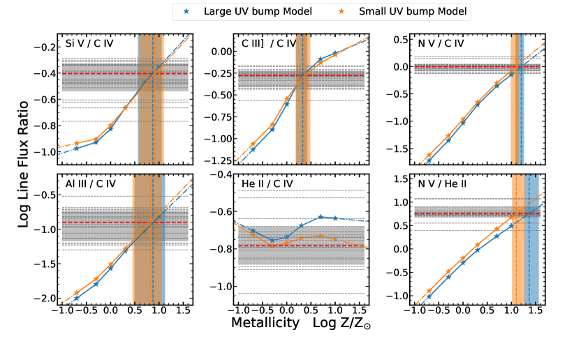
Figure 4: Illustration of converting line ratios to metallicities using photoionization models (Nagao et al., 2006). The blue and orange asterisks (and solid lines) represent the model predictions (and linear interpolation) from SEDs with large and small UV bumps, respectively. The dash-dotted lines are the extrapolation of these models. Each grey horizontal dashed line represents individual object in our sample, and red dashed lines represent the median ratio. The horizontal grey shaded areas are the range between 16th and 84th percentile of the line flux ratio distribution. The blue and orange vertical lines are the median metallicities indicated from the large and small UV bump models, respectively. The blue and orange shaded areas represent the range between 16th and 84th percentiles of the inferred metallicity distribution.

Next, we convert the line flux ratios to metallicities. We compare the median value of each line flux ratio with the photoionization predictions from the locally optimally emitting cloud (LOC) model (Baldwin et al., 1995). Hamann et al. (2002) and Nagao et al. (2006) carried out detailed simulations based on CLOUDY (Ferland et al., 1998) and studied how line flux ratios vary as a function of BLR metallicity. We utilize the model predictions in Table 10 of Nagao et al. (2006). Both small and large UV bump SED models are considered in our work.

Specifically, Nagao et al. (2006) provides the model predictions at ${\rm Z}/{\rm Z}_{\odot}=0.2,0.5,1.0,2.0,5.0,10.0,$ for N v$/$C IV, Si IV$/$C IV, C III]$/$C IV, Al III$/$C IV, and He ii$/$C IV. The N v$/$He ii ratio can be calculated using N v$/$C IV and He ii$/$C IV. Figure 4 illustrates how we estimate the metallicity from individual line ratios. We linearly interpolate (and extrapolate if necessary) the model predicted metallicity-line flux ratio curves and convert the line ratios to metallicity from the interpolation (extrapolation). Table 5 summarizes the estimated metallicities. We fail to convert He ii$/$C IV to metallicity because most of the measured He ii$/$C IV ratios do not overlap with the model predictions, which is also noted by Nagao et al. (2006).

Table 5: BLR metallicity of our sample estimated from median line flux ratios or flux ratios measured from the composite spectrum, using photoionization model predictions (Nagao et al., 2006).

Indicator	Metallicity ($Z/Z_{\odot}$)
	Large UV bump	Small UV bump
Median Metallicity of our sample
Si IV$/$C IV	$7.4_{-3.8}^{+3.9}$	$8.2_{-4.4}^{+4.3}$
C III]$/$C IV	$2.1_{-0.6}^{+0.5}$	$2.4_{-0.9}^{+0.7}$
Al III$/$C IV	$7.5_{-4.4}^{+5.9}$	$6.8_{-3.8}^{+4.7}$
N v$/$C IV	$16.0_{-4.0}^{+2.3}$	$12.5_{-3.0}^{+1.7}$
N v$/$He ii	$23.3_{-4.7}^{+13.6}$	$12.6_{-2.3}^{+6.4}$
Metallicity from the composite spectrum
Si IV$/$C IV	${4.7}_{-1.6}^{+1.8}$	${5.1}_{-1.8}^{+2.0}$
C III]$/$C IV	${1.9}_{-0.1}^{+0.1}$	${2.0}_{-0.1}^{+0.1}$
Al III$/$C IV	${7.7}_{-2.0}^{+2.0}$	${6.8}_{-1.6}^{+1.6}$
N v$/$C IV	${15.1}_{-3.5}^{+3.5}$	${11.9}_{-2.6}^{+2.6}$
N v$/$He ii	${23.4}_{-3.7}^{+3.7}$	${12.7}_{-1.8}^{+1.8}$

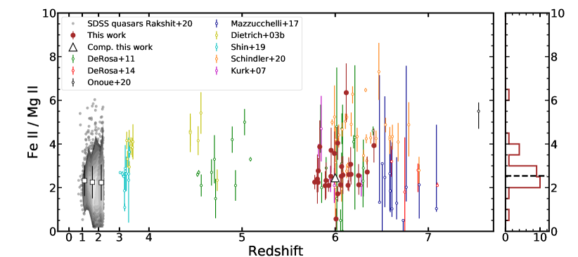
Figure 5: Fe ii$/$Mg ii ratios as a function of redshift. Different samples are indicated by different colors presented in the legend. The points represent individual measurement, while the triangles refer to the value of composite spectrum. The shaded area and the contours indicate the distribution of luminosity distribution matched low redshift SDSS quasars (Rakshit et al., 2020), and the squares refer to the median values in different redshift bins. We also display the histogram of Fe ii$/$Mg ii ratio distribution of our sample at the right panel, and the black dashed line refers to the median value. The x-axis is scaled for display purpose.

Converting line ratios to metallicities is subject to considerable systematic uncertainties. The conversion can be affected by factors such as the ionizing parameter, the hardness of the ionizing continuum, temperature, density, etc. (see Maiolino & Mannucci (2019) and reference therein). It is proposed that the relative abundance of N element can be used as metallicity diagnostics (e.g., Hamann et al., 2002), including N  III]$/$O III], N v/(C IV+O VI), N v/C IV, and N v/He ii. However, the line ratios involving the N element may be more related to N over-abundance rather than metallicity (Jiang et al., 2008). In addition, the line ratios that involve major UV lines, i.e., N v/C IV and N v/He ii, are sensitive to ionization parameter and shape of the ionizing continuum (Maiolino & Mannucci, 2019). Our results support this idea, as the inferred metallicities, ${\rm Z}_{\rm N\,{\rm V}/C\,{\rm IV}}$ and ${\rm Z}_{\rm N\,V/He\,II}$, are much higher than those from other indicators. On the other hand, this could also be a consequence of possible biases in our fitting, since Ly $\alpha$ often cannot be well modeled because of absorption in high-redshift quasars. But the median values of N v$/$C IV and N v$/$He ii agree with those measured from lower redshifts, suggesting that the Ly $\alpha$ absorption did not largely bias our N v measurements. Other preferred metallicity indicators are Si IV$/$C IV and Al III$/$C IV. These indicators do not involve the N element and are suggested to be more robust (Maiolino & Mannucci, 2019) since they are not sensitive to differences in the ionizing continuum (Nagao et al., 2006; Matsuoka et al., 2011; Maiolino & Mannucci, 2019). As for C III]$/$C IV, our results are similar to Nagao et al. (2006), who found $Z<2{Z_{\odot}}$ using C III]$/$C IV, reflecting the broad range of inferred metallicities from multiple line ratios using photoionization calculations.

In this work, we will not try to understand the discrepancy between each metallicity indicator, and neither will we draw any conclusion about which one should be adopted as the real metallicity. While individual line flux ratios do not provide accurate BLR metallicity estimates, we use the average metallicity over multiple line ratios to conclude that: 1) the BLR metallicity is at least supersolar even at $z\sim 6$; 2) for each of the metallicity indicators, there is no obvious trend with redshift up to $z\sim 6$. Our results are in agreement with the metallicity measurements in Jiang et al. (2007), who obtained metallicity estimate of $4Z_{\odot}$ at $z\sim 6$. These results suggest that the quasar BLRs are already metal enriched at $z\sim 6$, and the enrichment of the BLR metallicity must occur at earlier times and/or very quickly.

Table 6: Fe ii$/$Mg ii ratios using VW01 and T06 template

Name	Fe ii$/$Mg ii
	VW01	T06
J0002$+$2550	$2.77\pm 0.59$	$4.29\pm 1.11$
J0008$-$0626	$2.10\pm 0.29$	$3.81\pm 0.45$
J0050$+$3445	$2.55\pm 0.52$	$4.22\pm 0.98$
J0353$+$0104	$2.13\pm 0.42$	$3.02\pm 0.62$
J0810$+$5105	$2.33\pm 0.54$	$3.64\pm 0.92$
J0835$+$3217	$2.33\pm 0.82$	$3.99\pm 1.24$
J0836$+$0054	$3.87\pm 1.20$	$9.08\pm 1.84$
J0840$+$5624	$2.24\pm 0.44$	$4.02\pm 1.15$
J0841$+$2905	$2.52\pm 0.47$	$3.95\pm 0.81$
J0842$+$1218	$2.97\pm 0.46$	$5.06\pm 0.95$
J1044$-$0125	$2.25\pm 0.33$	$3.59\pm 0.96$
J1137$+$3549	$0.57\pm 0.48$	$0.74\pm 0.61$
J1148$+$0702	$2.72\pm 0.71$	$5.51\pm 1.00$
J1148$+$5251	$3.93\pm 0.78$	$6.97\pm 1.22$
J1207$+$0630	$1.72\pm 0.35$	$3.08\pm 0.67$
J1250$+$3130	$2.11\pm 0.23$	$4.31\pm 0.47$
J1257$+$6349	$3.57\pm 1.00$	$5.31\pm 1.72$
J1429$+$5447	$6.35\pm 1.34$	$13.12\pm 2.89$
J1436$+$5007	$2.39\pm 1.12$	$2.78\pm 1.86$
J1602$+$4228	$2.57\pm 0.86$	$3.92\pm 1.03$
J1609$+$3041	$2.60\pm 0.76$	$4.21\pm 1.12$
J1623$+$3112	$2.13\pm 0.45$	$3.05\pm 0.80$
J1630$+$4012	$2.52\pm 0.46$	$3.29\pm 0.89$
J2310$+$1855	$3.71\pm 1.03$	$5.30\pm 1.84$
P060+$2$4	$2.61\pm 0.46$	$4.14\pm 0.87$
P210+$2$7	$3.07\pm 0.79$	$4.29\pm 1.38$
P228+$2$1	$2.09\pm 0.66$	$3.09\pm 1.21$
P333+$2$6	$4.04\pm 0.77$	$6.10\pm 1.39$
Median	$2.54^{+1.12}_{-0.43}$	$4.08^{+1.36}_{-1.00}$
Composite	$2.45\pm 0.05$	$4.31\pm 0.11$

4.2 Fe ii$/$Mg ii

Core collapsed supernovae eject a comparable mass of Fe and Mg elements (e.g. Tsujimoto et al., 1995; Nomoto et al., 1997a) and produce a baseline [Fe/Mg] of roughly $-0.7\sim-0.4$ (Hamann & Ferland, 1999, and reference therein). On the other hand, SN Ia produce a larger amount of Fe relative to Mg and other $\alpha$ elements (e.g. Tsujimoto et al., 1995; Nomoto et al., 1997b). A rapid increase of the Fe$/$Mg abundance ratio is thus expected at the time when the progenitors of SN Ia began to explode (Venkatesan et al., 2004). The commonly quoted timescale of SN Ia, $t_{\rm Ia}$, is $\sim 1$ Gyr (Yoshii et al., 1996), which is close to the age of the universe at $z\sim 6.0$. Therefore, the Fe ii$/$Mg ii, used as the first order approximation of the Fe$/$Mg abundance ratio, can put important constraints on the star formation history at the early universe.

Figure 5 compares the Fe ii$/$Mg ii ratios of our sample with other studies from $z\sim 0.7$ to $z\sim 7.5$ (Dietrich et al., 2003b; Kurk et al., 2007; De Rosa et al., 2011, 2014; Mazzucchelli et al., 2017; Shin et al., 2019; Schindler et al., 2020; Onoue et al., 2020; Rakshit et al., 2020). For individual measurements, we only include literature samples that used the same Fe ii template (VW01) and the same Fe ii flux integration window ($2200<\lambda{\rm rest}<3090$ Å) as in the current work. In addition, we supplement a sample of low-redshift SDSS quasars from Data Release 14, whose spectral properties are measured by Rakshit et al. (2020). We select these SDSS quasars at $0.7<z<2.6$ that have similar luminosities as our sample quasars. We further require their spectral S/N$>10$. In addition to the luminosity-matched control sample, we also select SDSS quasars with a matched $L/L_{\rm Edd}$ as our Gemini sample. It shows that there is no obvious difference in the Fe ii$/$Mg ii distribution between luminosity-matched sample and $L/L_{\rm Edd}$-matched sample for the SDSS quasars. We thus use the luminosity-matched SDSS quasars as our main low-redshift control sample. There are also earlier studies that provided the Fe ii$/$Mg ii ratios using the T06 Fe ii templates. We present the comparison using the T06 template in Appendix. The measurements using both VW01 and T06 templates are summarized in Table 6.

As shown in Figure 5 and Table 6, the median Fe ii$/$Mg ii ratio of our sample ($2.54^{+1.12}_{-0.43}$) is consistent with measurements at low redshifts, e.g., low-redshift SDSS quasars and other samples. The median values of SDSS quasars in three redshift bins at $z\sim 1.20$, 1.68, and 2.16 are $2.32\pm 0.64$, $2.29\pm 0.72$, and $2.24\pm 0.82$, respectively. They are all consistent with our median value within $1\sigma$ uncertainty. The Fe ii$/$Mg ii ratio measured from our composite spectrum ($2.45\pm 0.05$) also confirms no evolution up to $z\sim 6$. Our results are also generally consistent with other studies for high-redshift quasars (Kurk et al., 2007; De Rosa et al., 2011, 2014; Mazzucchelli et al., 2017; Schindler et al., 2020).

There are two quasars in our sample, J1429+5447 and J1257+6349, labeled as weak-line quasars (WLQ) by Shen et al. (2019a). Their Fe ii$/$Mg ii ratios are 6.35 and 3.57, respectively. In their spectra, C IV is barely detected. Their equivalent widths are less than 10 Å, while Mg ii is detected. On the other hand, strong UV Fe ii emission is present, which is a typical feature of WLQs (Wu et al., 2011). WLQs may have an intrinsically different Fe ii$/$Mg ii distribution and thus complicate the interpretation. Indeed, J1429+5447 has the highest Fe ii$/$Mg ii ratio in our sample, while J1257+6349 is marginally within the 16th$-$84th range. If we exclude these two WLQs, the median Fe ii$/$Mg ii ratio decreases from 2.54 to 2.52. Therefore, the two WLQs in our sample have a negligible effect on our conclusions.

The Fe$/$Mg element abundance ratio is not the only factor that affects the Fe ii$/$Mg ii ratio. Detailed photoionization calculations suggest that the Fe ii$/$Mg ii ratio has a strong dependence on the velocity of microturbulence (e.g. Verner et al., 2003; Baldwin et al., 2004; Sarkar et al., 2021; Panda, 2021). Though the preferred turbulence velocity is different among different studies, the existence of microturbulence is found to be the key to reproduce the observed strength and shape of the Fe ii UV bump (Verner et al., 2003; Baldwin et al., 2004; Sarkar et al., 2021). The calculated Fe ii$/$Mg ii ratio varies with the turbulence velocity: one dex difference in the turbulence velocity will cause $0.3\sim 0.5$ dex difference in Fe ii$/$Mg ii (Verner et al., 2003). On the other hand, one dex difference in the Fe abundance will result in $\sim 0.3$ dex difference in Fe ii$/$Mg ii (Verner et al., 2003). Even if the affect of microturbulence is determined, Fe ii$/$Mg ii also correlates with the $L/L_{\rm Edd}$ (e.g. Dong et al., 2009; Sameshima et al., 2017; Shin et al., 2021). All of these largely complicates the interpretation of the Fe ii$/$Mg ii ratio. A more detailed and consistent study that determines the effect of the microturbulence is needed to fully understand the problem.

If we assume that the Fe ii$/$Mg ii line flux ratio reflects the Fe$/\alpha$ abundance ratio, the lack of redshift evolution of Fe ii$/$Mg ii at $z\sim 6$ (and even $z\sim 7$, combined with other studies) seems to challenge the commonly quoted timescale of SN Ia $t_{\rm Ia}$. The timescale $t_{\rm Ia}$ can vary with star formation history (e.g., Matteucci & Recchi, 2001). In the case of elliptical galaxies in which star formation was initially very efficient and stopped after a short duration ($<0.4$ Gyr), $t_{\rm Ia}$ can be as short as $0.3$ Gyr. For an instantaneous star formation, $t_{\rm Ia}$ is only $\sim 40$ Myr. Observational studies of SN Ia delay time (same as $t_{\rm Ia}$) distribution also found that the rate of SN Ia follows the form of $t^{-1}$ and the highest SN Ia rate occurs at the time as short as 0.2 Gyr after the initial star burst (e.g., Totani et al., 2008; Maoz et al., 2012, 2014; Wiseman et al., 2021). Therefore, the lack of the Fe ii$/$Mg ii  evolution at $z\sim 6$ suggests that the initial star formation happened at least before $z\sim 8.1$ ($t_{\rm Ia}\sim 0.3$ Gyr) or $z\sim 7.3$ ($t_{\rm Ia}\sim 0.2$ Gyr) for these quasars.

Finally, we discuss several additional factors that could bias our measurements and/or produce the scatter seen in our measurements. In addition to the choice of the Fe ii template and the Fe ii flux integration window, other possible factors include the fitting range, inclusion of narrow Mg ii components, etc. We use the composite spectrum to fit the $2200<\lambda_{\rm rest}<3300$ Å range instead of the windows adopted in our fiducial spectral analysis (§3.1), because in many studies their spectra only cover this wavelength range. We find that the derived Fe ii$/$Mg ii ratio is 2.85 if adopting the new fitting windows. We also perform a test using a single broad Gaussian for Mg ii, which only changes the results by less than 5%. Therefore, we conclude that the uncertainties in our fitting methodology do not bias our conclusions.

5 Discussion

We do not find an apparent redshift evolution of the quasar BLR metallicity at redshift up to $z\sim 6$. This is in contrast to star-forming galaxies and DLAs in which a strong redshift evolution of metallicity at $0<z<3.5$ has been firmly established (e.g., Maiolino et al., 2008; Mannucci et al., 2009). To explain this difference, many studies attribute the non-evolution in quasars to selection biases (Juarez et al., 2009; Maiolino & Mannucci, 2019), such that only the most massive quasars at high redshift are observed. Combined with the BH mass-BLR metallicity relation discovered at lower redshifts (Matsuoka et al., 2011; Xu et al., 2018), we are selectively observing quasar BLRs with high metallicities at $z\sim 6$.

In order to test if the above selection bias can explain the non-evolution in BLR metallicities, we compare our results with previous measurements in quasars with similar BH masses. Xu et al. (2018) adopted the average metallicity indicated by Si IV/C IV and N v/C IV as their final metallicity for the BH mass-metallicity relation. They also linearly interpolate (or extrapolate) model predictions as what we did. The only difference is that they compiled the three models in Hamann et al. (2002) to estimate $Z_{\rm N\,V/C\,IV}$, The models share the same assumptions of relative metal abundance scale as Nagao et al. (2006), and take the same solar abundance values from Grevesse & Anders (1989). There are 16 quasars in our sample that have both Si IV$/$C IV and N v$/$C IV measurements. They are directly compared with Xu et al. (2018) following the same recipes of metallicity estimation. The results are shown in Figure 6. At fixed BH masses, the metallicities at $z\sim 6$ from our sample are consistent with those at $2<z<5$ from Xu et al. (2018). We present a linear regression fit to both $2<z<5$ (Xu et al., 2018) and $z\sim 6$. For the case of $2<z<5$, we choose the mass range of ${\rm Log}M_{\rm BH}/M_{\odot}>8.6$, where the mass-metallicity relation seems to be linear. The relation is expressed in the form of ${\rm Log}Z/Z_{\odot}=m\times({\rm Log}(M_{\rm BH}/M_{\odot})-{\rm Log}(M_{0}/M_{\odot}))+b$. $M_{0}$ is taken as 9.2 to make the mass range symmetric in log space to better constrain the difference in the intercepts. The best-fit slope and intercept are $0.49\pm 0.05$ and $0.93\pm 0.02$, respectively. The best-fit slope is different from what was presented in Xu et al. (2018), since we exclude the points below $10^{8.6}M_{\odot}$. For the case of $z\sim 6$, we fix the slope to be the same in the case of $2<z<5$ because of the limited mass range and small number of points. The best-fit intercept is $0.90\pm 0.04$, consistent with that of the low-redshift case within a 1$\sigma$ uncertainty. This indicates that there is no obvious evolution in the BH mass-BLR metallicity relation over $2<z<6$. Changing the mass cut range in the $2<z<5$ case or the value of $M_{0}$ does not change our results. Therefore, we conclude that selection bias is unable to explain the non-evolution of the quasar BLR metallicities. In fact, our comparisons with low-redshift quasar samples matched in luminosity (hence approximately in BH mass) already ruled out the selection bias as the main reason for the lack of evolution in BLR metallicities.

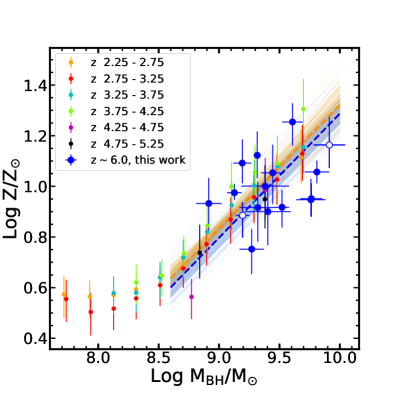
Figure 6: The BH mass-BLR metallicity relation at $z\sim 6.0$ (blue) using our sample, compared with the results at $2.5<z<5.0$ (Xu et al., 2018). The blue open circles represent the BH mass measured from C IV. The thin orange lines are randomly selected linear regression fits to all points in the range of ${\rm Log}M_{\rm BH}/M_{\odot}>8.6$ in the case of $2<z<5$ (Xu et al., 2018). The orange dashed line refers to the median of the distribution. The blue thin and dashed lines are the result of this work.

The BH mass-BLR metallicity relation is very different from the stellar mass-metallicity relation in star-forming galaxies. The BLR metallicities are typically $0.3\sim 1$ dex higher than those in star-forming galaxies (Xu et al., 2018). In addition, there is a strong redshift evolution in the galaxy mass-metallicity relation. One explanation is that quasar host galaxies are distinct from star-forming galaxies in terms of metallicity and its redshift evolution (Xu et al., 2018). However, studies of AGN narrow line region (NLR) metallicity do not support this explanation. The scale of the NLR is comparable to that of the host galaxy (e.g., Bennert et al., 2006). Recent studies of Type II AGNs have reached a consensus that the galaxy mass-NLR metallicity relation is similar to that for star-forming galaxies (Matsuoka et al., 2018a; Dors et al., 2019). There is also tentative evidence (see Maiolino & Mannucci (2019) and reference therein) that the AGN NLR metallicity has a similar redshift evolution as star-forming galaxies over $0<z<2$ (Coil et al., 2015; Dors et al., 2019) (see Figure 3 in Dors et al. (2019)).

An alternative explanation is that the timescale for the BLR gas to get metal enriched is very short. Although the origin of the BLR and its high metallicity is unclear, this is a viable scenario, since the gas density of the BLR is high, and the BLR can experience a rapid star formation and metal enrichment. Some studies explored in-situ star formation models in the BLR (Shlosman & Begelman, 1989; Collin & Zahn, 1999; Wang et al., 2011), where self-gravity causes instability and fragmentation of the accretion disk at outer region (e.g. beyond the self-gravity radius, $\sim 0.1$pc (Collin & Zahn, 1999)). One possible picture is that these fragments will finally collapse and result in local star formation (Collin & Zahn, 1999). The supernovae explosion from these in-situ stars can inject adequate amounts of metals into the BLR and enrich the gas to as high as $10\sim 20$ ${\rm Z}_{\odot}$. On the other hand, the gas mass in the BLR is only up to a few time of $10^{4}$ ${\rm M}_{\odot}$ (Baldwin et al., 2003), therefore the enrichment timescale can be as short as $10^{4}$ yrs (Juarez et al., 2009).

Using different methods to estimate quasar metallicity other than broad emission line ratios would also be valuable. One possible approach is to use quasar intrinsic absorption lines (see references in Hamann & Ferland, 1999). Many studies confirm that the metallicities indicated from either broad or narrow absorption lines, are also super solar (e.g., Arav et al., 1999, 2020; Gabel et al., 2006). In our sample, many quasars exhibit diverse intrinsic absorption features. However, the typical spectral resolution and the S/N of our sample make it difficult to deploy this method.

6 Summary

We have performed detailed spectral analysis of 33 quasars at $5.7<z<6.4$ to study their BLR metallicities. These quasars were drawn from a sample of 50 quasars observed using Gemini GNIRS. The NIR spectra cover $0.9-2.5\mu m$. The C IV or Mg ii line flux can be robustly measured in the 33 quasars. We used different line flux ratios as metallicity diagnostics, including Si IV$/$C IV, C III]$/$C IV, Al III$/$C IV, He ii$/$C IV, N v$/$C IV, and N v$/$He ii. The Fe ii$/$Mg ii ratios were also measured. Our main conclusions are as below.

1. We compared different metallicity diagnostic line flux ratios with earlier samples measured at various redshifts. The median ratios of our sample are consistent with the luminosity-matched sample at $2<z<4.5$, suggesting no obvious redshift evolution in BLR metallicity up to $z\sim 6$. The high S/N median composite spectrum from our sample confirms this non-evolution.

2. We converted the observed line flux ratios to metallicities using photoionization model predictions. The typical metallicity of our sample depends on the indicator used, but is at least a few times the solar value. Our results imply the gas in the BLR is already highly enriched at $z\sim 6$.

3. We compared the Fe ii$/$Mg ii ratios with those measured for quasars at other redshifts. There is no evidence of redshift evolution in the Fe ii$/$Mg ii ratio in quasars up to $z\sim 6$, suggesting rapid star formation happened at earlier epochs.

4. We found a consistent relation between the black hole mass and the BLR metallicity at $z\sim 6$ as seen in low-redshift quasars, and ruled out selection biases as the main cause for the non-evolution of quasar BLR metallicity.

Our results confirmed similar earlier studies with smaller sample sizes and/or less coverage of various UV broad emission lines. The confirmation of no evolution in the BLR metallicity and the Fe/$\alpha$ ratio up to $z\sim 6$ strongly constrains star formation and metal enrichment in the vicinity of the SMBH. Better metallicity diagnositics can further solidify these results, and refine the metallicity measurements in individual quasars.

Appendix Appendix Effects of the Fe ii template on the Fe ii$/$Mg ii ratio

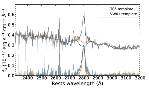
Figure 7: An example (J1250+3130) of our fits using two Fe ii templates, VW01 (blue) and T06 (orange). The upper spectrum in black is the original spectrum, and the lower spectrum (in blue and orange) represents the pseudo-continuum (VW01 and T06, respectively) subtracted Mg ii profile. We overplot the best-fit Gaussian models using thick blue and orange lines. The fitting results using the VW01 template have systematically lower Mg ii fluxes than using T06.

We investigate the Fe ii$/$Mg ii ratios using the T06 template to model Fe ii. We follow the same fitting approach but replace the VW01 template with the T06 template. Figure 7 compares the two Fe ii templates with an example to illustrate the differences between the fitting results. Using the T06 template produces higher Fe ii and lower Mg ii fluxes, thus higher Fe ii$/$Mg ii ratio. Table 6 includes Fe ii$/$Mg ii ratios measured for our sample using the T06 template.

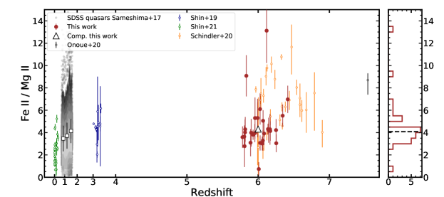
Figure 8: Same as Figure 5 but for the results derived using the T06 template. The results for SDSS quasars measured using the T06 templates are from Sameshima et al. (2017).

Figure 8 compares our measurements with other samples using the T06 template (Sameshima et al., 2017; Shin et al., 2019, 2021; Schindler et al., 2020). The median values of SDSS quasars in three redshift bins ($0.7<z<1.1$, $1.1<z<1.4$, $1.4<z<1.7$) are $3.46\pm 1.15$, $3.72\pm 1.16$, and $4.14\pm 1.09$, respectively. Our median value, $4.08^{+1.36}_{-1.00}$, is consistent with those for low redshift SDSS quasars. In addition, the value measured from our high S/N composite spectrum (4.31$\pm 0.11$) is generally in line with this result. Similar to our fiducial measurements using the VW01 Fe ii template, we find no obvious redshift evolution in the Fe ii$/$Mg ii ratio using the T06 template. For consistency check, we compare our Fe ii$/$Mg ii measurements with other works using T06 (Schindler et al., 2020) for those overlapped objects. There are three overlapped objects with Schindler et al. (2020): J0842$+$1218, J1148$+$0702, and J2310$+$1855. For two of them, the measurements are consistent within 1$\sigma$ uncertainty, while for the other object it shows large difference, indicating possible systematics in spectral decomposition or data reduction. A uniform pipeline is needed in the future to reduce any systematics.

References

- Arav et al. (1999) Arav, N., Korista, K. T., de Kool, M., Junkkarinen, V. T., & Begelman, M. C. 1999, ApJ, 516, 27
- Arav et al. (2020) Arav, N., Xu, X., Kriss, G. A., et al. 2020, A&A, 633, A61
- Bañados et al. (2018) Bañados, E., Carilli, C., Walter, F., et al. 2018, ApJ, 861, L14
- Bañados et al. (2016) Bañados, E., Venemans, B. P., Decarli, R., et al. 2016, ApJS, 227, 11
- Bañados et al. (2019) Bañados, E., Rauch, M., Decarli, R., et al. 2019, ApJ, 885, 59
- Baldwin et al. (1995) Baldwin, J., Ferland, G., Korista, K., & Verner, D. 1995, ApJ, 455, L119
- Baldwin et al. (2003) Baldwin, J. A., Ferland, G. J., Korista, K. T., Hamann, F., & Dietrich, M. 2003, ApJ, 582, 590
- Baldwin et al. (2004) Baldwin, J. A., Ferland, G. J., Korista, K. T., Hamann, F., & LaCluyzé, A. 2004, ApJ, 615, 610
- Barth et al. (2003) Barth, A. J., Martini, P., Nelson, C. H., & Ho, L. C. 2003, ApJ, 594, L95
- Bennert et al. (2006) Bennert, N., Jungwiert, B., Komossa, S., Haas, M., & Chini, R. 2006, A&A, 459, 55
- Bian et al. (2017) Bian, F., Kewley, L. J., Dopita, M. A., & Blanc, G. A. 2017, ApJ, 834, 51
- Coil et al. (2015) Coil, A. L., Aird, J., Reddy, N., et al. 2015, ApJ, 801, 35
- Collin & Zahn (1999) Collin, S., & Zahn, J.-P. 1999, A&A, 344, 433
- De Rosa et al. (2011) De Rosa, G., Decarli, R., Walter, F., et al. 2011, ApJ, 739, 56
- De Rosa et al. (2014) De Rosa, G., Venemans, B. P., Decarli, R., et al. 2014, ApJ, 790, 145
- Dietrich et al. (2003a) Dietrich, M., Appenzeller, I., Hamann, F., et al. 2003a, A&A, 398, 891
- Dietrich et al. (2003b) Dietrich, M., Hamann, F., Appenzeller, I., & Vestergaard, M. 2003b, ApJ, 596, 817
- Dietrich et al. (2003c) Dietrich, M., Hamann, F., Shields, J. C., et al. 2003c, ApJ, 589, 722
- Dong et al. (2009) Dong, X.-B., Wang, T.-G., Wang, J.-G., et al. 2009, ApJ, 703, L1
- Dors et al. (2015) Dors, O. L., Cardaci, M. V., Hägele, G. F., et al. 2015, MNRAS, 453, 4102
- Dors et al. (2019) Dors, O. L., Monteiro, A. F., Cardaci, M. V., Hägele, G. F., & Krabbe, A. C. 2019, MNRAS, 486, 5853
- Fan et al. (2006) Fan, X., Strauss, M. A., Richards, G. T., et al. 2006, AJ, 131, 1203
- Ferland et al. (1998) Ferland, G. J., Korista, K. T., Verner, D. A., et al. 1998, PASP, 110, 761
- Gabel et al. (2006) Gabel, J. R., Arav, N., & Kim, T.-S. 2006, ApJ, 646, 742
- Grevesse & Anders (1989) Grevesse, N., & Anders, E. 1989, in American Institute of Physics Conference Series, Vol. 183, Cosmic Abundances of Matter, ed. C. J. Waddington, 1–8
- Guo et al. (2018) Guo, H., Shen, Y., & Wang, S. 2018, PyQSOFit: Python code to fit the spectrum of quasars, , , ascl:1809.008
- Guo et al. (2020) Guo, Y., Maiolino, R., Jiang, L., et al. 2020, ApJ, 898, 26
- Hamann & Ferland (1993) Hamann, F., & Ferland, G. 1993, ApJ, 418, 11
- Hamann & Ferland (1999) —. 1999, ARA&A, 37, 487
- Hamann et al. (2002) Hamann, F., Korista, K. T., Ferland, G. J., Warner, C., & Baldwin, J. 2002, ApJ, 564, 592
- Jiang et al. (2008) Jiang, L., Fan, X., & Vestergaard, M. 2008, ApJ, 679, 962
- Jiang et al. (2007) Jiang, L., Fan, X., Vestergaard, M., et al. 2007, AJ, 134, 1150
- Jiang et al. (2016) Jiang, L., McGreer, I. D., Fan, X., et al. 2016, ApJ, 833, 222
- Juarez et al. (2009) Juarez, Y., Maiolino, R., Mujica, R., et al. 2009, A&A, 494, L25
- Kelly (2007) Kelly, B. C. 2007, ApJ, 665, 1489
- Kurk et al. (2007) Kurk, J. D., Walter, F., Fan, X., et al. 2007, ApJ, 669, 32
- Ledoux et al. (2006) Ledoux, C., Petitjean, P., Fynbo, J. P. U., Møller, P., & Srianand, R. 2006, A&A, 457, 71
- Maiolino & Mannucci (2019) Maiolino, R., & Mannucci, F. 2019, A&A Rev., 27, 3
- Maiolino et al. (2008) Maiolino, R., Nagao, T., Grazian, A., et al. 2008, A&A, 488, 463
- Mannucci et al. (2009) Mannucci, F., Cresci, G., Maiolino, R., et al. 2009, MNRAS, 398, 1915
- Maoz et al. (2012) Maoz, D., Mannucci, F., & Brandt, T. D. 2012, MNRAS, 426, 3282
- Maoz et al. (2014) Maoz, D., Mannucci, F., & Nelemans, G. 2014, ARA&A, 52, 107
- Mason et al. (2015) Mason, R. E., Rodríguez-Ardila, A., Martins, L., et al. 2015, ApJS, 217, 13
- Matsuoka et al. (2018a) Matsuoka, K., Nagao, T., Marconi, A., et al. 2018a, A&A, 616, L4
- Matsuoka et al. (2011) Matsuoka, K., Nagao, T., Marconi, A., Maiolino, R., & Taniguchi, Y. 2011, A&A, 527, A100
- Matsuoka et al. (2018b) Matsuoka, Y., Iwasawa, K., Onoue, M., et al. 2018b, ApJS, 237, 5
- Matsuoka et al. (2019) Matsuoka, Y., Onoue, M., Kashikawa, N., et al. 2019, ApJ, 872, L2
- Matteucci & Recchi (2001) Matteucci, F., & Recchi, S. 2001, ApJ, 558, 351
- Mazzucchelli et al. (2017) Mazzucchelli, C., Bañados, E., Venemans, B. P., et al. 2017, ApJ, 849, 91
- Møller et al. (2013) Møller, P., Fynbo, J. P. U., Ledoux, C., & Nilsson, K. K. 2013, MNRAS, 430, 2680
- Mortlock et al. (2011) Mortlock, D. J., Warren, S. J., Venemans, B. P., et al. 2011, Nature, 474, 616
- Nagao et al. (2006) Nagao, T., Marconi, A., & Maiolino, R. 2006, A&A, 447, 157
- Nakajima et al. (2013) Nakajima, K., Ouchi, M., Shimasaku, K., et al. 2013, ApJ, 769, 3
- Nakajima et al. (2012) —. 2012, ApJ, 745, 12
- Nomoto et al. (1997a) Nomoto, K., Hashimoto, M., Tsujimoto, T., et al. 1997a, Nucl. Phys. A, 616, 79
- Nomoto et al. (1997b) Nomoto, K., Iwamoto, K., Nakasato, N., et al. 1997b, Nucl. Phys. A, 621, 467
- Onoue et al. (2020) Onoue, M., Bañados, E., Mazzucchelli, C., et al. 2020, ApJ, 898, 105
- Panda (2021) Panda, S. 2021, A&A, 650, A154
- Prochaska et al. (2013) Prochaska, J. X., Hennawi, J. F., Lee, K.-G., et al. 2013, ApJ, 776, 136
- Rafelski et al. (2014) Rafelski, M., Neeleman, M., Fumagalli, M., Wolfe, A. M., & Prochaska, J. X. 2014, ApJ, 782, L29
- Rakshit et al. (2020) Rakshit, S., Stalin, C. S., & Kotilainen, J. 2020, ApJS, 249, 17
- Reed et al. (2019) Reed, S. L., Banerji, M., Becker, G. D., et al. 2019, MNRAS, 487, 1874
- Richards et al. (2006) Richards, G. T., Lacy, M., Storrie-Lombardi, L. J., et al. 2006, ApJS, 166, 470
- Salviander et al. (2007) Salviander, S., Shields, G. A., Gebhardt, K., & Bonning, E. W. 2007, ApJ, 662, 131
- Sameshima et al. (2017) Sameshima, H., Yoshii, Y., & Kawara, K. 2017, ApJ, 834, 203
- Sarkar et al. (2021) Sarkar, A., Ferland, G. J., Chatzikos, M., et al. 2021, ApJ, 907, 12
- Schindler et al. (2020) Schindler, J.-T., Farina, E. P., Bañados, E., et al. 2020, ApJ, 905, 51
- Shen et al. (2011) Shen, Y., Richards, G. T., Strauss, M. A., et al. 2011, ApJS, 194, 45
- Shen et al. (2016) Shen, Y., Brandt, W. N., Richards, G. T., et al. 2016, ApJ, 831, 7
- Shen et al. (2019a) Shen, Y., Wu, J., Jiang, L., et al. 2019a, ApJ, 873, 35
- Shen et al. (2019b) Shen, Y., Hall, P. B., Horne, K., et al. 2019b, ApJS, 241, 34
- Shin et al. (2019) Shin, J., Nagao, T., Woo, J.-H., & Le, H. A. N. 2019, ApJ, 874, 22
- Shin et al. (2021) Shin, J., Woo, J.-H., Nagao, T., Kim, M., & Bahk, H. 2021, ApJ, 917, 107
- Shlosman & Begelman (1989) Shlosman, I., & Begelman, M. C. 1989, ApJ, 341, 685
- Tang et al. (2019) Tang, J.-J., Goto, T., Ohyama, Y., et al. 2019, MNRAS, 484, 2575
- Totani et al. (2008) Totani, T., Morokuma, T., Oda, T., Doi, M., & Yasuda, N. 2008, PASJ, 60, 1327
- Tremonti et al. (2004) Tremonti, C. A., Heckman, T. M., Kauffmann, G., et al. 2004, ApJ, 613, 898
- Tsujimoto et al. (1995) Tsujimoto, T., Nomoto, K., Yoshii, Y., et al. 1995, MNRAS, 277, 945
- Tsuzuki et al. (2006) Tsuzuki, Y., Kawara, K., Yoshii, Y., et al. 2006, ApJ, 650, 57
- Vanden Berk et al. (2001) Vanden Berk, D. E., Richards, G. T., Bauer, A., et al. 2001, AJ, 122, 549
- Venkatesan et al. (2004) Venkatesan, A., Schneider, R., & Ferrara, A. 2004, MNRAS, 349, L43
- Verner et al. (2003) Verner, E., Bruhweiler, F., Verner, D., Johansson, S., & Gull, T. 2003, ApJ, 592, L59
- Vestergaard & Peterson (2006) Vestergaard, M., & Peterson, B. M. 2006, ApJ, 641, 689
- Vestergaard & Wilkes (2001) Vestergaard, M., & Wilkes, B. J. 2001, ApJS, 134, 1
- Wang et al. (2021) Wang, F., Yang, J., Fan, X., et al. 2021, ApJ, 907, L1
- Wang et al. (2009) Wang, J.-G., Dong, X.-B., Wang, T.-G., et al. 2009, ApJ, 707, 1334
- Wang et al. (2011) Wang, J.-M., Ge, J.-Q., Hu, C., et al. 2011, ApJ, 739, 3
- Wang et al. (2020) Wang, S., Shen, Y., Jiang, L., et al. 2020, ApJ, 903, 51
- Willott et al. (2007) Willott, C. J., Delorme, P., Omont, A., et al. 2007, AJ, 134, 2435
- Willott et al. (2010) Willott, C. J., Delorme, P., Reylé, C., et al. 2010, AJ, 139, 906
- Wiseman et al. (2021) Wiseman, P., Sullivan, M., Smith, M., et al. 2021, MNRAS, 506, 3330
- Woo et al. (2018) Woo, J.-H., Le, H. A. N., Karouzos, M., et al. 2018, ApJ, 859, 138
- Wu et al. (2011) Wu, J., Brandt, W. N., Hall, P. B., et al. 2011, ApJ, 736, 28
- Wu et al. (2015) Wu, X.-B., Wang, F., Fan, X., et al. 2015, Nature, 518, 512
- Xu et al. (2018) Xu, F., Bian, F., Shen, Y., et al. 2018, MNRAS, doi:10.1093/mnras/sty1763
- Yang et al. (2019) Yang, J., Wang, F., Fan, X., et al. 2019, AJ, 157, 236
- Yang et al. (2020) —. 2020, ApJ, 897, L14
- Yang et al. (2021) —. 2021, arXiv e-prints, arXiv:2109.13942
- Yoshii et al. (1996) Yoshii, Y., Tsujimoto, T., & Nomoto, K. 1996, ApJ, 462, 266
- Yu et al. (2021) Yu, Z., Martini, P., Penton, A., et al. 2021, MNRAS, 507, 3771
- Zahid et al. (2014) Zahid, H. J., Dima, G. I., Kudritzki, R.-P., et al. 2014, ApJ, 791, 130
- Zou et al. (2021) Zou, S., Jiang, L., Shen, Y., et al. 2021, ApJ, 906, 32