Order Fractionalization in a Kitaev-Kondo model

Abstract

We describe a mechanism for order fractionalization in a two-dimensional Kondo lattice model, in which electrons interact with a gapless spin liquid of Majorana fermions described by the Yao-Lee (YL) model. When the Kondo coupling to the conduction electrons exceeds a critical value, the model develops a superconducting instability into a state with a a spinor order parameter with charge $e$ and spin $S=1/2$. The broken symmetry state develops a gapless Majorana Dirac cone in the bulk. By including an appropriate gauge string, we can show that the charge $e$, spinorial order develops off-diagonal long range order that allows electrons to coherently tunnel arbitrarily long distances through the spin liquid.

I Introduction

One of the fascinating properties of quantum materials is the phenomenon of fractionalization, whereby excitations break-up into emergent particles with fractional quantum numbers. Well-established examples of fractionalization include anyons in the quantum Hall effect and the break-up of magnons into $S=1/2$ spinons in the one dimensional Heisenberg spin chain. There is great current interest in the possibility that new patterns of fractionalization can lead to new kinds of quantum phases and quantum materials.

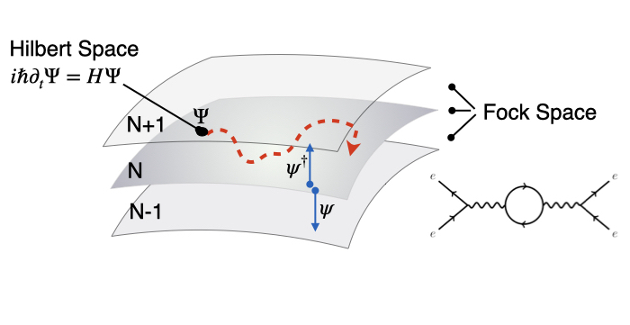
Figure 1: In second quantization, the “physical” Hilbert space of definite particle numbers is expanded to a Fock space that allows the description of particle fields.

There are some important parallels between second quantization and fractionalization. We recall that even though a many-body electron wave function evolves in a Hilbert space of rigorously fixed particle number, physical quantities such as density

$$\rho({\bf x})=\sum_{j}\delta({\bf x}-{\bf x}_{j})\longrightarrow\psi^{\dagger}({\bf x})\psi({\bf x}),$$ (1)

factorize into creation and annihilation operators $\psi^{\dagger}(x)$ and $\psi(x)$ that link Hilbert spaces of different particle number (see Fig. 1). Thus the description of particles requires an expansion of the Hilbert space into a larger Fock space. Normally we take this for granted - we are quite accustomed to the notion that photons create particle-hole pairs, content in the understanding that gauge invariance ($\psi\rightarrow e^{i\alpha(x)}\psi$, $A\rightarrow A+\nabla\alpha(x)$) preserves particle number.

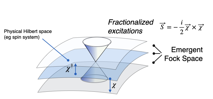
Figure 2: Fractionalization involves the break-up of physical operators such as spin, into excitations with fractional quantum numbers which require an emergent Fock space for their description.

In a similar fashion, fractionalization can be regarded as an emergent second-quantization, in which the microscopic variables, such as the spin, factorize into operators that describe fractionalized quasiparticles (see Fig. 2), thus in a spin liquid a spin flip creates a pair of spinons. Such fractionalized particles live within an emergent Fock space, and like their vacuum counterparts, move under the influence of a gauge field which preserves the constraints of the physical Hilbert space.

One of the most dramatic manifestations of second-quantization is the formation of superfluid condensates, in which the field operators develop off-diagonal long-range order (ODLRO), manifested as a factorization of the density matrix in terms of the order parameter $\langle\psi({\bf x})\rangle=\Psi({\bf x})$,

$$\langle\psi({\bf x})\psi^{\dagger}({\bf y})\rangle\xrightarrow[]{|{\bf x}-{\bf y}|\rightarrow\infty}\Psi({\bf x})\Psi({\bf y})^{*}.$$ (2)

The description of superconductors is more subtle, for now the condensate field operator carries charge and transforms under a gauge transformation $\hat{\psi}(x)\rightarrow e^{i\alpha(x)}\hat{\psi}(x)$, $\vec{A}\rightarrow\vec{A}+\nabla\alpha$, so that $\langle\Psi(x)\rangle$ vanishes after averaging over the gauge fields, a result known as Elitzur’s theorem. A sharper definition of ODLRO[1] then requires the introduction of a gauge invariant boson field[2]

$$\hat{\psi}_{N}({\bf x})=\hat{\psi}({\bf x})e^{-i\int d^{3}r\vec{A}({\bf r})\cdot\vec{E}_{cl}({\bf r}-{\bf x})},$$ (3)

where $\vec{E}_{cl}({\bf r})$ is the classical electric field of a point charge at the origin, i.e $\nabla\cdot E_{cl}=\delta({\bf r})$, $\vec{E}_{cl}({\bf r})=\hat{\bf r}/(4\pi r^{2})$), and $\vec{A}$ is the fluctuating, quantum vector potential. Off-diagonal long-range order is then defined by

$$\langle\hat{\psi}_{N}({\bf x})\hat{\psi}_{N}^{\dagger}({\bf y})\rangle\xrightarrow{|{\bf x}-{\bf y}|\rightarrow\infty}\Psi({\bf x})\Psi({\bf y})^{*},$$ (4)

where $\Psi({\bf x})=\langle\hat{\psi}_{N}({\bf x})\rangle$. The massive nature of the vector potential inside a Meissner phase, guarantees that this result holds true, even when quantum fluctuations are included. These considerations lead us to ask: if fractionalization is a kind of emergent second-quantization, is there a fractionalized analog of superfluidity or superconductivity?

Early theoretical studies of a possible interplay between fractionalization and broken symmetry were inspired by the RVB-theory of cuprate superconductivity[3, 4, 5]; in these papers fractionalization appears under the guise of “spin-charge separation”. In particular, the appearance of a charge $e$ boson in the slave-boson decomposition of the electron operator $c^{\dagger}_{j\sigma}\rightarrow f^{\dagger}_{j\sigma}b_{j}$ raised the early intriguing possibility of novel order parameters associated with spin-charge separation. Although the presence of an emergent $U(1)$ gauge field associated with spin-charge separation appeared to forstall a superconducting, charge $e$ condensate, it was soon realized[6, 7] that there might be a topological effect. In particular, the topological interplay of the electromagnetic and emergent $U(1)$ gauge fields, Wen and Lee[6] identified a two-parameter family of vortices and subsequently, Sachdev proposed a possible stablization of $h/e$ vortices[7] near a superconductor, pseudo-gap phase boundary. The modern term “fractionalization” appeared in a second-generation of theories[8, 9] that were inspired by the pseudo-gap phase of cuprate superconductors. These theories identified the fractionalization of electrons and spins with an emergent $Z_{2}$ gauge field. Senthil and Fisher[9] introduced the term “vison” to describe the vortices of the $Z_{2}$ field. In their theory, the development of a gap in the vison spectrum gives rise to a novel fractionalized insulator gapped vison excitations.

Our paper returns to these early lines of investigation, taking crucial advantage of the Kitaev approach to introduce a new platform for the discussion, in the form of a family of models which control the gauge fields that are at the heart of fractionalization. The Kitaev approach with its static $Z_{2}$ gauge fields now makes it explicitly clear that fractionalization is physical. This then leads us to reconsider the question of whether the condensation of fractionalized bosons can actually give rise to novel forms of order parameter? This could happen, for instance if a spinon binds to an electron. The resulting order parameter has the potential to carry fractional quantum numbers with novel order-parameter topologies and symmetries, giving rise to a conjectured “order fractionalization”[10].

Here, we explore the idea of order fractionalization within the context of the Kondo lattice model. The Kondo lattice has a venerable history: first written down by Kasuya in 1955[11], later proposed in the 1970s by Mott and Doniach[12, 13] to explain heavy fermion materials. The Kondo lattice describes a lattice of local moments, coupled to conduction electrons via an antiferromagnetic super-exchange of strength $J$. When $J$ is sufficiently large, the local moments become screened by conduction electrons, liberating their entangled spin degrees of freedom into the conduction sea as a narrow band of “heavy electrons”.

From a modern perspective, the Kondo lattice effect can be understood as a spin fractionalization of localized moments. In a heavy Fermi liquid, local moments split into spin 1/2 heavy fermions, conventionally described as a bilinear of S=1/2 “Dirac” fermions[14, 15, 16, 17, 18],

$$\vec{S}({\bf x}_{j})\rightarrow f^{\dagger}_{j\alpha}\left(\frac{\vec{\sigma}}{2}\right)_{\alpha\beta}f_{j\beta}.$$ (5)

In this scenario, a spin flip creates a pair of “spinons” moving in an emergent $U(1)$ gauge field which enforces their incompressibility[19]. When the Kondo effect takes place, the coherent exchange of spin between the electron and spin fluid Higgses the $U(1)$ gauge field, locking it to the electromagnetic field and converting the neutral spinons into charged heavy fermions[20]. This “Dirac fractionalization” of spins provides a natural way to understand the expansion of the Fermi surface in the Kondo lattice, described by Oshikawa’s theorem[21, 22].

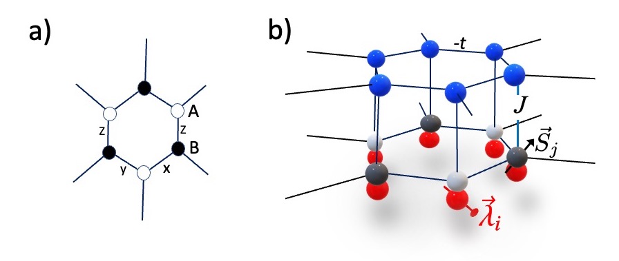
Figure 3: Schematic of the Kitaev Kondo model showing a), the x, y and z bonds of the lattice and b) the structure. The lower layer is a Yao-Lee spin liquid with gapless spin ($\vec{S}_{j}$) and gapped orbital degrees of freedom ($\vec{\lambda}_{i}$). The upper layer is a honeycomb lattice of conduction electrons, coupled to the spin liquid via a Kondo interaction.

Here we study an unconventional spin fractionalization into Majorana fermions, first proposed in[23, 24]

$$\vec{S}({\bf x}_{j})\rightarrow-\frac{i}{2}(\vec{\chi}_{j}\times\vec{\chi}_{j}),$$ (6)

where $\vec{\chi}_{j}=(\chi^{1}_{j},\chi^{2}_{j},\chi^{3}_{j})$ is a spin-1 majorana that moves in a $Z_{2}$ gauge field. In this alternate scenario, a spin flip produces a pair of majoranas. Majorana fractionalization gives rise to a gapless band of neutral excitations, and has been proposed as a driver of odd-frequency pairing[23] and the origin of Kondo insulators with neutral Fermi surfaces[24, 26, 27].

A novelty of our work, is the Kondo-coupling of electrons to a gapless spin liquid in which Majorana fractionalization is rigorously established. We combine a variant of the Kitaev honeycomb model[28], called the Yao-Lee model[29, 30, 31, 32, 33, 34], with a corresponding lattice of mobile electrons. Like the Kitaev model, the Yao-Lee model is exactly solvable, which allows a nonperturbative treatment of the fractionalization, i.e the strongest correlations in the model. The weaker Kondo exchange is then treated withing mean field approximation in the manner of Bogoluibov-de-Gennes theory. Unlike the original Kitaev model, in which spin excitations create gapped $Z_{2}$ vortices[28], the Yao-Lee model describes a spin liquid in which spin flips fractionalize into gapless Majorana fermions, leaving the static $Z_{2}$ gauge field unaffected. This radically affects the character of the Kondo interaction between the conduction electrons and the local moments, opening up the possibility of a fractionalized order parameter formed from a pair condensation of electrons and Majorana fermions.

In the Yao Lee model, the motion of the Majorana fermions is described by the Hamiltonian

$$H_{YL}=K\sum_{<i,j>}u_{ij}(i\vec{\chi}_{i}\cdot\vec{\chi}_{j}),$$ (7)

where $u_{ij}=\pm 1$ is the static gauge field. The exchange-coupling of a Yao-Lee spin liquid to electrons on an adjacent honeycomb layer (Fig. 3) now forms a Kondo lattice in which the absence of gauge fluctuations establishes an order-fractionalized state[10] in which electrons and majoranas combine into charge $e$, $S=1/2$ bosons

$$\hat{v}({\bf x}_{j})=\bigl{(}\vec{\sigma}_{\alpha\beta}\cdot\vec{\chi}_{j}\bigr{)}c_{j\beta}=\begin{pmatrix}\hat{v}_{j\uparrow}\\ \hat{v}_{j\downarrow}\end{pmatrix},$$ (8)

where $c_{j}$ is an electron operator at site $j$. When this boson condenses, it gives rise to a state in which triplet pairs have fractionalized into condensed bosonic spinors, forming a well-defined order parameter with charge e and spin 1/2.

Since the fractionalized fields $\vec{\chi}_{j}$ and $\hat{v}(x)$ carry a $Z_{2}$ charge, a gauge invariant definition of off-diagonal long range order follows a similar procedure to a superconductor, introducing a string of $Z_{2}$ gauge fields,

$${\cal P}({\bf x}_{i},{\bf y}_{j})=\prod_{l\in P_{{j\rightarrow i}}}u_{(l+1,l)}$$ (9)

along a path $P_{j\rightarrow i}$ linking sites $j$ and $i$, giving rise to the asymptotic factorization

$$\langle v({{\bf x}}){\cal P}({\bf x},{\bf y})v^{\dagger}({{\bf y}})\rangle\xrightarrow[]{|{\bf x}-{\bf y}|\rightarrow\infty}v({\bf x})v^{\dagger}({\bf y}).$$ (10)

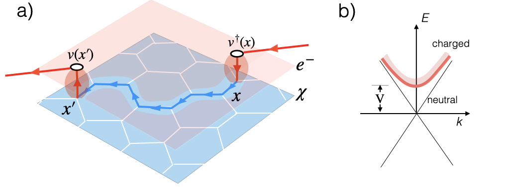
Figure 4: a) Development of a charge $e$ condensate $v(x)$ permits the coherent tunneling of electrons through the spin-liquid over arbitrary distances. b) The mismatch between the three Majorana components of the spin liquid and the four Majorana components of the conduction electrons (59) leads to a decoupled “neutral” conduction electron Majorana Dirac cone with a gap to charged electron excitations.

As in a superconductor, the $Z_{2}$ vortices, or “visons” are absent in the ground state, so one can adopt an axial gauge where the $u_{(i,j)}=1$ and the string becomes unity. The development of this off-diagonal long range order with fractional quantum numbers constitutes order fractionalization[10, 36].

One of the most dramatic consequences of this off-diagonal long-range order, is that electrons can tunnel over arbitrarily large distances through the spin liquid (Fig. 4a). The amplitude $\Sigma(x^{\prime},x)$ for this process is directly proportional to the spinor order at the entry and exit points $x$ and $x^{\prime}$,

$$\Sigma(x^{\prime},x)\sim v(x^{\prime})\frac{1}{|x^{\prime}-x|^{2}}v^{\dagger}(x).$$ (11)

The long-range coherence of this process reflects the order-fractionalization. The neutral character of the Majoranas in the spin fluid has two interesting consequences: first, it means that when electrons emerge from this tunneling process, they can reappear into the conduction fluid as either electrons, or holes, giving rise to both normal and Andreev scattering processes. Secondly, the mismatch between the quantum numbers of the electrons and the Majorana fermions then gaps out three Majorana components of the conduction sea, leaving behind a neutral Majorana cone of conduction-like excitations (Fig. 4b). The sharp coherence of this neutral band reflects the phase coherence of the charge $e$ spinor order.

If we sample the spinor field locally, we can construct a composite order parameter

$$\langle\hat{v}^{T}({\bf x})i\sigma_{2}\vec{\sigma}v({\bf x})\rangle \propto \langle c_{\uparrow}({\bf x})c_{\downarrow}({\bf x})\vec{S}({\bf x})\rangle$$ (12)

$$= {\Psi}({\bf x})(\hat{d}_{1}({\bf x})+i\hat{d}_{2}({\bf x})),$$ (13)

representing the local binding of a Cooper pair to a spin where $\hat{d}^{1}$ and $\hat{d}^{2}$ are members of an orthogonal triad of unit vectors $(\hat{d}^{1},\hat{d}^{2},\hat{d}^{3})$. However, this is not the primary order parameter of the physics, as can be seen by observing that the gap in the spectrum is proportional to $|v|$, rather than $|v|^{2}$.

The structure of this paper is as follows. Section II introduces the Kitaev Kondo Model. Section III reviews the properties of the Yao-Lee spin liquid. Section IV introduces the mean-field theory for the order-fractionalizing transition. Section V discusses the quantum critical transition at half filling and the first order order fractionalizing transition that develops with finite doping. Section VI discusses the nature of the off-diagonal fractionalized long-range order. Section VII discusses the nature of the triplet pairing, and its odd-frequency character. Section VIII discusses the phase diagram and long-wavelength action. Finally, Section IX discusses the broader implications of our results.

II Kitaev-Kondo model

Coupling a Yao-Lee spin liquid to a conduction sea, forms a Kondo lattice with Hamiltonian $H=H_{C}+H_{YL}+H_{K}$ (see Fig. 3), where

$$H_{C} = -t\sum_{<i,j>}(c^{\dagger}_{i\sigma}c_{j\sigma}+{\rm H.c})-\mu\sum_{j}c^{\dagger}_{j\sigma}c_{j\sigma},$$ (14)

$$H_{YL} = (K/2)\sum_{<i,j>}(\vec{\sigma}_{i}\cdot\vec{\sigma}_{j})\lambda_{i}^{\alpha_{ij}}\lambda^{\alpha_{ij}}_{j},$$ (15)

$$H_{K} = J\sum_{j}\vec{S}_{j}\cdot c^{\dagger}_{j}\vec{\sigma}c_{j}.$$ (16)

Here $\langle i,j\rangle$ denotes a pair of neighboring sites, with $i$ on the even (A) and $j$ on the odd (B) sublattice. $H_{C}$ is a tight-binding model of conduction electrons moving on honeycomb lattice with hopping matrix element $-t$. $H_{YL}$ is the Yao-Lee model, a version of the Kitaev honeycomb model in which each site has both an orbital degree of freedom, denoted by three Pauli orbital $\lambda^{a}_{j}$($a=1,2,3$) operators and a spin degree of freedom, denoted by the Pauli matrices $\vec{\sigma}_{j}$. The ${\vec{S}}_{j}\equiv\vec{\sigma}_{j}/2$ are the normalized spins for the localized moments and the $\alpha_{ij}=x,y,z$ along the x,y and z bonds of the honeycomb lattice (Fig. 3). Finally, $H_{K}$ describes an antiferromagnetic exchange interaction between the electrons and the spin liquid.

Several earlier variants of Kitaev Kondo lattices have been considered, including models that couple the original, spin-gapped Kitaev spin liquid to a conduction sea[32, 38, 39], and models that couple a Yao-Lee spin liquid to a conduction sea via an anisotropic, octupolar coupling[40]. The current model builds on these earlier treatments, isotropically coupling electrons to a solvable gapless spin-liquid to preserve the $SU(2)$ spin symmetry, leading to a fluid in which crucially, the gapped visons decouple from the low energy spin and charge fluctuations.

III The Yao-Lee Spin Liquid

We begin by recapitulating the key features of the Yao-Lee spin liquid[29, 30, 31, 32, 33, 34]. The first step is to transmute the spin and orbital operators into fermions, expanding the Hilbert space into a Fock space by adding two ancilliary Majorana fermions $\Phi^{S}_{j}$ and $\Phi^{T}_{j}$, equivalent to one ancilliary qubit, at each site. We use the normalizing convention $(\Phi^{S,T}_{j})^{2}=\frac{1}{2}$ throughout this paper for all majoranas. The spin and orbital majoranas are defined as a fusion of the Pauli operators with the ancillars[41]

$$\chi_{j}^{\alpha}=\Phi^{S}_{j}\sigma_{j}^{\alpha},\qquad b^{a}=\Phi^{T}_{j}\lambda^{a}_{j}.$$ (17)

These satisfy canonical anticommutation algebras $\{\chi^{a}_{j},\chi^{b}_{j}\}=\{b^{a}_{j},b^{b}_{j}\}=\delta^{ab}\delta_{ij}$ and $\{\chi^{a}_{j},b^{b}_{k}\}=0$. Using the fact that $\sigma^{x}\sigma^{y}\sigma^{z}=\lambda^{x}\lambda^{y}\lambda^{z}=i$, we obtain the reverse transformations

$$\Phi_{j}^{S}=-2i\chi_{j}^{1}\chi_{j}^{2}\chi_{j}^{3},\qquad\Phi_{j}^{T}=-2ib_{j}^{1}b_{j}^{2}b_{j}^{3},$$ (18)

which enable us to write the spins and orbitals as

$$\vec{\sigma}_{j} = 2\Phi_{j}^{S}\vec{\chi}_{j}=-{i}\vec{\chi}_{j}\times\vec{\chi}_{j},$$ (19)

$$\vec{\lambda}_{j} = 2\Phi_{j}^{T}\vec{b}_{j}=-{i}\vec{b}_{j}\times\vec{b}_{j},$$ (20)

where we use vector notation $\vec{\chi}_{j}=(\chi^{1}_{j},\chi^{2}_{j},\chi^{3}_{j})$ and $\vec{b}_{j}=(b^{1}_{j},b^{2}_{j},b^{3}_{j})$. It follows that $\sigma^{a}_{j}\lambda_{j}^{\alpha}=-2i\hat{D}_{j}\chi^{a}_{j}b_{j}^{\alpha}$, where

$$\hat{D}_{j}=-2i\Phi_{j}^{S}\Phi_{j}^{T}=8i\chi_{j}^{1}\chi_{j}^{2}\chi_{j}^{3}b_{j}^{1}b_{j}^{2}b_{j}^{3}.$$ (21)

Now $\hat{D}_{j}$, with eigenvalues $D_{j}=\pm 1$, commutes with $H$, and the constraint $D_{j}=1$ selects a physical Hilbert space

$$|\psi_{p}\rangle=\prod_{j}\frac{1}{2}(1+D_{j})|\psi\rangle.$$ (22)

in which

$$\sigma_{j}^{a}\lambda_{j}^{\alpha}=-2i\chi_{j}^{a}b^{\alpha}_{j},$$ (23)

which enables us to rewrite (15) in the expanded Fock space of majoranas as

$$H_{YL}=K\sum_{<i,j>}\hat{u}_{ij}(i\vec{\chi}_{i}\cdot\vec{\chi}_{j}).$$ (24)

Here, the $i$ and $j$ sites are on the A and B sublattices respectively, and the $\hat{u}_{i,j}=-2ib_{i}^{\alpha_{ij}}b_{j}^{\alpha_{ij}}$ are gauge fields that live on the bonds, with eigenvalues $u_{ij}=\pm 1$. (Note the negative sign in the bond operator, which simplifies later calculation of string variables). The remarkable feature of Kitaev models, making them so useful for our analysis, is that the gauge fields $\hat{u}_{ij}$ are completely static variables, rigorously commuting with $H$ and the constraint operators $D_{j}$.

Like the Kitaev honeycomb model, $H_{YL}$ describes a $Z_{2}$ spin liquid with the gauge symmetry

$$\vec{\chi}_{j}\rightarrow Z_{j}\vec{\chi}_{j},\quad\hat{u}_{ij}\rightarrow Z_{i}\hat{u}_{ij}Z_{j},\qquad(Z_{j}=\pm 1).$$ (25)

The product

$$\hat{W}_{\rm p}=\prod_{<l+1,l>\in\rm p}\hat{u}_{(l+1,l)}=\prod_{j\in\rm p}\lambda^{a_{j}}_{j}$$ (26)

around a hexagonal plaquette $p$, where the $a_{j}$ denote the directions exterior to the plaquette, commutes with $H$ and the $D_{j}$, forming a set of gauge-invariant constants describing static $Z_{2}$ fluxes (visons). Note our use of the parentheses around the indices of the $\hat{u}_{(l+1,l)}$, which re-arranges the subscripts so that the A sublattice index is first.

In the ground state, the eigenvalues $W_{p}=1$ on every plaquette while plaquettes where $W_{p}=-1$ describe gapped “vison” excitations. Since a $\vec{\lambda}_{j}$ flips a bond, it creates two visons, so the orbital degrees of freedom are gapped. This is then a Higgs phase for the $Z_{2}$ fields, in which the $Z_{2}$ gauge field has become massive. However, unlike the Kitaev honeycomb model, there are three gapless $\vec{\chi}$ majoranas which describe the fractionalization of the spins $\vec{S}_{j}=-(i/2)\vec{\chi}_{j}\times\vec{\chi}_{j}$. The action of $\vec{S}_{j}$ does not create visons, leading to a spin liquid with gapless spin excitations.

Although the vector Majorana fermions are not gauge invariant, they can be made so by attaching a gauge string to them to create a $Z_{2}$-neutral field

$$\vec{\chi}_{N}(i)=\vec{\chi}(i){\cal P}({\bf x}_{i},-\infty)$$ (27)

where ${\cal P}({\bf x},{\bf y})$ is the $Z_{2}$ string defined in (9) .

It is convenient to choose a axial gauge in which the $u^{x,y}_{ij}=1$ along the x and y bonds, leaving the z-bonds as the dependent variables. Visons are present at a plaquette containing two $u^{z}_{ij}$ of opposite sign, so we can set all bonds to unity, $u_{ij}=1$, causing the strings to vanish, establishing an equivalence

$$\vec{\chi}_{N}(i)\sim\vec{\chi}(i).$$ (28)

in the axial gauge. The key point is that in the ground state the majoranas $\chi_{j}$ can be treated as physical fields that describe the gapless spin excitations. We can also transform back to the original spin variables, writing the majorana in terms of a Jordan-Wigner string

$$\frac{1}{\sqrt{2}}\vec{\chi}({j})=\vec{S}(j)\left(\prod_{l\in P_{j}}\lambda^{z}(l)\right)\times\left\{\begin{array}[]{cc}\lambda^{x}(j),&(j\in B),\cr\lambda^{y}(j),&(j\in A),\end{array}\right.$$ (29)

where the string takes a product of $\lambda^{z}(j)$ along the path $P$ consisting of sites to the left and below site $j$ (see appendix A).

In the axial-gauge (24) becomes

$$H_{YL}=\frac{K}{2}\sum_{i,j}\Big{[}\gamma({\bf R}_{i}-{\bf R}_{j})\vec{\chi}_{A}({i})\cdot\vec{\chi}_{B}({j})+{\rm H.c}\Big{]}.$$ (30)

where ${\bf R}_{i}$ is the location of the unit cell. The hopping amplitude $\gamma({\bf R})=i(\delta_{{\bf R},0}+\delta_{{\bf R},{\bf R}_{1}}+\delta_{{\bf R},{\bf R}_{2}})$, where ${\bf R}_{1,2}=(\mp\frac{\sqrt{3}}{2},\frac{3}{2})$ are the Bravais lattice vectors. We now Fourier transform the Majorana fields, defining a vector majorana on each sublattice

$$\chi_{{\bf k}\Lambda}=\begin{pmatrix}\chi^{1}_{\Lambda}({\bf k})\cr{\chi^{2}_{\Lambda}}({\bf k})\cr{\chi^{3}_{\Lambda}}({\bf k})\end{pmatrix}=\frac{1}{\sqrt{N}}\sum_{j}\begin{pmatrix}\chi^{1}_{\Lambda}(j)\cr\chi^{2}_{\Lambda}(j)\cr\chi^{3}_{\Lambda}(j)\end{pmatrix}e^{-i{\bf k}\cdot{\bf R}_{j}},\quad\Lambda\in(A,B),$$ (31)

where $N$ is the number of unit cells. Finally, combining $\chi_{{\bf k}A}$ and $\chi_{{\bf k}B}$ into a six component vector

$$\chi_{{\bf k}}=\begin{pmatrix}\chi_{{\bf k}A}\cr\chi_{{\bf k}B}\end{pmatrix},$$ (32)

the Hamiltonian becomes

$$H_{YL}=\frac{K}{2}\sum_{{\bf k}\in{\hexagon}}{\chi_{{\bf k}}}^{\dagger}\begin{pmatrix}0&\gamma_{\bf k}\ \underline{1}\cr\gamma^{*}_{{\bf k}}\ \underline{1},&0\end{pmatrix}\chi_{{\bf k}}$$ (33)

where $\gamma_{{\bf k}}=i(1+e^{i{\bf k}\cdot{\bf R}_{1}}+e^{i{\bf k}\cdot{\bf R}_{2}})$ and the momentum sum runs over the original hexagonal Brillouin zone ($\hexagon$). Now the real nature of the Majorana fermions means that ${\chi^{a}_{{\bf k}\Lambda}}^{\dagger}={\chi^{a}_{-{\bf k}\Lambda}}$, so the two halves of the Brillouin zone are equivalent, allowing us to truncate the Brillouin zone to a triangular region (${\triangleleft}$) that surrounds the Dirac cone at $K$ and spans half the hexagonal Brillouin zone (see Fig.5). In terms of this reduced Brillouin zone, the real-space fields can be written

$$\chi^{a}_{\Lambda}(j)=\frac{1}{\sqrt{N}}\sum_{{\bf k}\in{\triangleleft}}\left(\chi^{a}_{{\bf k}\Lambda}e^{i{\bf k}\cdot{\bf R}_{j}}+{\chi^{a}}^{\dagger}_{{\bf k}\Lambda}e^{-i{\bf k}\cdot{\bf R}_{j}}\right),$$ (34)

and the Hamiltonian becomes

$$H_{YL}=K\sum_{{\bf k}\in{\triangleleft}}{\chi_{{\bf k}}}^{\dagger}(\vec{\gamma}_{{\bf k}}\cdot\vec{\alpha})\chi_{{\bf k}},$$ (35)

where $\vec{\gamma}_{{\bf k}}=({\rm Re}\gamma_{{\bf k}},-{\rm Im}\gamma_{{\bf k}},0)$ and the $\vec{\alpha}=(\alpha_{1},\alpha_{2},\alpha_{3})\otimes 1_{[3]}$ are Pauli matrices acting in sublattice space.

Diagonalizing (35) then gives

$$H_{YL}=\sum_{{\bf k}\in{\raisebox{-0.7113pt}{${\triangleleft}$}}}\epsilon_{s}({\bf k})({\vec{\eta}_{{\bf k}1}}^{\dagger}\cdot{\vec{\eta}}_{{\bf k}1}-{\vec{\eta}_{{\bf k}2}}^{\dagger}\cdot\vec{\eta}_{{\bf k}2}),$$ (36)

where $\epsilon_{s}({\bf k})=K|\gamma_{{\bf k}}|$, describing a Dirac cone of majorana excitations centered at $K$. The quasiparticle operators are given by

$$\vec{\eta}_{{\bf k}1} = u_{{\bf k}}\vec{\chi}_{{\bf k}A}+v_{{\bf k}}\vec{\chi}_{{\bf k}B},$$ (37)

$$\vec{\eta}_{{\bf k}2} = -v^{*}_{{\bf k}}\vec{\chi}_{{\bf k}A}+u^{*}_{{\bf k}}\vec{\chi}_{{\bf k}B},$$ (38)

where $u_{{\bf k}}={1}/{\sqrt{2}}$ and $v_{{\bf k}}=\gamma_{{\bf k}}/(\sqrt{2}|\gamma_{{\bf k}}|)$. In the ground-state $|\phi_{YL}\rangle$ all negative energy states are filled,

$$|\phi_{YL}\rangle=\prod_{a\in\{1,3\},{\bf k}\in{\triangleleft}}{\eta^{a}}^{\dagger}_{{\bf k}2}|0\rangle.$$ (39)

The presence of a triplet of gapless ?ajoranas means that the energy cost of visons is three times larger than in the Kitaev spin liquid, and given by approximately $0.4K$ per vison pair[28].

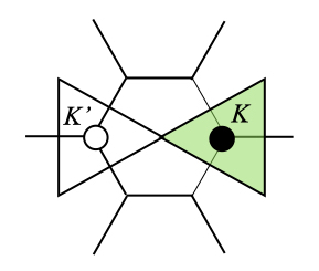
Figure 5: The hexagonal Brillouin zone of the honeycomb lattice, where nodes of the dispersion $\epsilon({\bf k})=|\gamma_{{\bf k}}|$ lie at the vertices $K$ and ${K}^{\prime}$. Majorana excitations are independently defined over one half the Brillouin zone, described by the green triangle centered at ${K}$.

IV Majorana Kondo Effect

IV.1 Mean-field Hamiltonian

We now examine the effect of the Kondo interaction on the spin liquid. If we rewrite this interaction in terms of the majoranas $\vec{\chi}_{j}$, it becomes

$$H_{K} = J\sum_{j}(c^{\dagger}_{j}\vec{\sigma}c_{j})\cdot\left(-\frac{i}{2}\vec{\chi}_{j}\times\vec{\chi}_{j}\right)$$ (40)

$$= -\frac{J}{2}\sum_{j}c^{\dagger}_{j}\left[\left(\vec{\sigma}\cdot\vec{\chi}_{j}\right)^{2}-\frac{3}{2}\right]c_{j}.$$ (41)

The last term in (40) can be absorbed by a shift in the electron chemical potential, allowing us to write

$$H_{K}\equiv-\frac{J}{2}\sum_{j}\left(\hat{v}_{j}^{\dagger}\hat{v}_{j}\right),$$ (42)

where $\hat{v}$ is a $S=1/2$, charge $e$ spinor boson given originally in Eq.(8),

$$\hat{v}_{j}=\bigl{(}\vec{\sigma}_{\alpha\beta}\cdot\vec{\chi}_{j}\bigr{)}c_{j\beta}=\begin{pmatrix}\hat{v}_{j\uparrow}\\ \hat{v}_{j\downarrow}\end{pmatrix}.$$ (43)

Thus the fractionalization of the spins into majoranas transforms the Kondo interaction into an attraction that favors the condensation of charge e spinor boson.

At temperatures low enough to suppress visons, there are no residual $Z_{2}$ gauge field fluctuations, and we can consequently treat the $\hat{v}_{j}$ as a gauge neutral field. Taking advantage of the bilinear form of the Kondo interaction, we now carry out a Hubbard-Stratonovich transformation

$$H_{K} = -\frac{J}{2}\sum_{j}c^{\dagger}_{j}\left[\left(\vec{\sigma}\cdot\vec{\chi}_{j}\right)^{2}\right]c_{j}$$ (44)

$$\longrightarrow \sum_{j}\biggl{(}\biggl{[}V^{\dagger}_{j}(\vec{\sigma}\cdot\chi_{j})c_{j}+{\rm H.c}\biggr{]}+2\frac{V^{\dagger}_{j}V_{j}}{J}\biggr{)}$$ (45)

where

$$V_{j}=\begin{pmatrix}V_{j\uparrow}\cr V_{j\downarrow}\end{pmatrix}\equiv-\frac{J}{2}v_{j}$$ (46)

is a spinor order parameter. The equivalence between $V_{j}\equiv-(J/2)v_{j}$ holds at the saddle point.

It proves convenient to make a global gauge transformation on the even (A) sublattice, $(c_{A\sigma},c_{B\sigma})\rightarrow(-ic_{A\sigma},c_{B\sigma})$ and similarly, $(V_{A\sigma},V_{B\sigma})\rightarrow(-iV_{A\sigma},V_{B\sigma})$. The conduction electron Hamiltonian then takes the form

$$H_{C}=-it\sum_{<i,j>}(c^{\dagger}_{i\sigma}c_{j\sigma}-{\rm H.c})-\mu\sum_{j}c^{\dagger}_{j\sigma}c_{j\sigma},$$ (47)

In this gauge at $\mu=0$ the conduction and Majorana Hamiltonian have the same form, with opposite signs. Moreover, in the lowest energy configuration the Kondo bosons $\hat{v}_{j}$ then conveniently condense into a uniform condensate.

The hybridization with the spin liquid induces triplet pairing, so to proceed further, we define a 4-component Balian-Werthammer spinor on each sublattice

$$\psi_{{\bf k}\Lambda}=\begin{pmatrix}c_{{\bf k}\Lambda\uparrow}\cr c_{{\bf k}\Lambda\downarrow}\cr-c^{\dagger}_{-{\bf k}\Lambda\downarrow}\cr c^{\dagger}_{-{\bf k}\Lambda\uparrow}\end{pmatrix},\qquad(\Lambda=A,B).$$ (48)

We then merge the two sublattice spinors into an 8-component operator

$$\psi_{{\bf k}}=\begin{pmatrix}\psi_{{\bf k}A}\cr\psi_{{\bf k}B}\end{pmatrix}.$$ (49)

In this basis, the sublattice ($\alpha$) charge ($\tau$) and spin ($\sigma$) operators are denoted by three sets of Pauli operators given by the outer products

$$\vec{\alpha}_{[8]} \equiv \vec{\alpha}_{[2]}\otimes 1_{[2]}\otimes 1_{[2]},$$ (50)

$$\vec{\tau}_{[8]} \equiv 1_{[2]}\otimes\vec{\tau}_{[2]}\otimes 1_{[2]},$$ (51)

$$\vec{\sigma}_{[8]} \equiv 1_{[2]}\otimes 1_{[2]}\otimes\vec{\sigma}_{[2]},$$ (52)

where the bracketed subscripts denoting the dimensions of the operator will be dropped in future. We shall use the transposed Pauli matrices for the isospin degrees of freedom $\vec{\tau}_{[2]}\equiv\vec{\sigma}^{T}_{[2]}=(\sigma_{1},-\sigma_{2},\sigma_{3})$, a choice that simplifies later expressions. In this notation,

$$H_{C}=\sum_{{\bf k}\in{\triangleleft}}\psi^{\dagger}_{{\bf k}}(-t\vec{\gamma}_{{\bf k}}\cdot\vec{\alpha}-\mu\tau_{3})\psi_{{\bf k}}.$$ (53)

We now introduce a four-component spinor to describe the Kondo hybridization,

$${\cal V}_{\Lambda}=\begin{pmatrix}V_{\Lambda\uparrow}\cr V_{\Lambda\downarrow}\cr-V^{*}_{\Lambda\downarrow}\cr V^{*}_{\Lambda\uparrow}\end{pmatrix}={\rm V}_{\Lambda}{\cal Z}_{\Lambda},$$ (54)

where

$${\cal Z}_{\Lambda} = \frac{1}{\sqrt{2}}\begin{pmatrix}z_{\Lambda\uparrow}\cr z_{\Lambda\downarrow}\cr-z^{*}_{\Lambda\downarrow}\cr z^{*}_{\Lambda\uparrow}\end{pmatrix}$$ (55)

is normalized to unity ${\cal Z}_{\Lambda}^{\dagger}{\cal Z}_{\Lambda}=1$, and we use a Roman V_Λ to denote the magnitude of the hybridization. The hybridized Kondo term then becomes

$$H_{K}=\sum_{\Lambda=A,B}\left(\sum_{{\bf k}\in{\triangleleft}}\biggl{[}(\psi^{\dagger}_{{\bf k}\Lambda}\vec{\sigma}{\cal V}_{\Lambda})\cdot\vec{\chi}_{{\bf k}\Lambda}+{\rm H.c}\biggr{]}+2N\frac{{\rm V}_{\Lambda}^{2}}{J}\right).$$ (56)

We shall focus on the uniform case, where ${\cal V}_{A}={\cal V}_{B}={\cal V}$, which creates the largest hybridization gap. Combining (53) (56) and (35), the mean-field Hamiltonian can be compactly written as

$$H=\sum_{{\bf k}\in{\triangleleft}}\Psi^{\dagger}_{{\bf k}}\begin{pmatrix}-t(\vec{\gamma}_{{\bf k}}\cdot\vec{\alpha})-\mu\tau_{3}&\vec{\sigma}{\cal V}\cr{\cal V}^{\dagger}\vec{\sigma}&K(\vec{\gamma}_{{\bf k}}\cdot\vec{\alpha})\end{pmatrix}\Psi_{{\bf k}}+4N\frac{{\rm V}^{2}}{J}$$ (57)

where

$$\Psi_{{\bf k}}=\begin{pmatrix}\psi_{{\bf k}}\cr\chi_{{\bf k}}\end{pmatrix},$$ (58)

where $\psi_{{\bf k}}$ is defined in (49) and $\chi_{{\bf k}}$ is defined in (32). In the off-diagonal components of (57) we have used the short-hand $\psi^{\dagger}_{{\bf k}}\vec{\sigma}{\cal V}{\chi}_{{\bf k}}\equiv\psi^{\dagger}_{{\bf k}}(\vec{\sigma}\cdot\vec{\chi}_{{\bf k}}){\cal V}$ and $\vec{\chi}^{\dagger}_{{\bf k}}{\cal V}^{\dagger}\vec{\sigma}\psi_{{\bf k}}\equiv{\cal V}^{\dagger}({\vec{\chi}}^{\dagger}_{{\bf k}}\cdot\vec{\sigma})\psi_{{\bf k}}$.

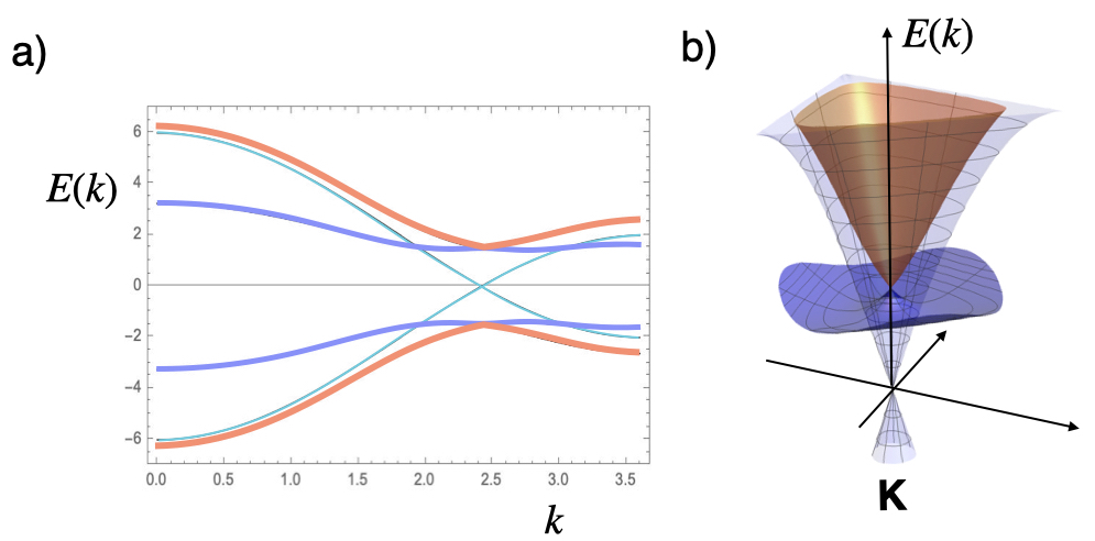
Figure 6: a) Spectrum of the Kitaev Kondo lattice for $\mu=0$, taking units $K=1$, $t=2K$ and ${\rm V}=1.5K$. Thick orange lines denote gapped conduction electron lines, thick blue lines denote the gapped Majorana spin excitations while while thin blue lines denote the single gapless Majorana conduction band. b) Schematic three dimensional plot of spectrum in the vicinity of the $K$ point.

IV.2 The case of half filling ($\mu=0$).

If we now split the conduction sea into scalar and vector components

$${\psi}^{0}_{{\bf k}\Lambda} = {\cal Z}^{\dagger}\cdot\psi_{{\bf k}\Lambda},$$ (59)

$$\vec{\psi}_{{\bf k}\Lambda} = {\cal Z}^{\dagger}\cdot\vec{\sigma}\cdot\psi_{{\bf k}\Lambda},$$ (60)

then from (56) we can decouple

$$(\psi^{\dagger}_{{\bf k}\Lambda}\vec{\sigma}{\cal V})\cdot\vec{\chi}_{{\bf k}\Lambda}={\rm V}(\psi^{\dagger}_{{\bf k}\Lambda}\vec{\sigma}{\cal Z})\cdot\vec{\chi}_{{\bf k}\Lambda}={\rm V}(\vec{\psi}^{\dagger}_{{\bf k}\Lambda}\cdot\vec{\chi}_{{\bf k}\Lambda}).$$ (61)

In other words, only the vector Majorana components of the conduction sea hybridize with the spin liquid, and the scalar part is unhybridized. At particle-hole symmetry $\mu=0$, the Hamiltonian decouples into a gapless scalar conduction sea and gapped vector sea of excitations

$$H = \sum_{{\bf k}\in{\triangleleft}}\psi^{\dagger}_{0{\bf k}}(-t\vec{\gamma}_{{\bf k}}\cdot\vec{\alpha})\psi_{0{\bf k}}+4N\frac{{\rm V}^{2}}{J}$$ (62)

$$+ \sum_{{\bf k}\in{\triangleleft}}\begin{pmatrix}\vec{\psi}^{\dagger}_{{\bf k}}&\vec{\chi}^{\dagger}_{{\bf k}}\end{pmatrix}\begin{pmatrix}-t\vec{\gamma}_{{\bf k}}\cdot\vec{\alpha}&{\rm V}\cr{\rm V}&K\vec{\gamma}_{{\bf k}}\cdot\vec{\alpha}\end{pmatrix}\begin{pmatrix}\vec{\psi}_{{\bf k}}\cr\vec{\chi}_{{\bf k}}\end{pmatrix}.$$ (63)

The fourteen eigenvalues of this Hamiltonian involve a single Dirac cone with the two eigenvalues $\pm\epsilon_{c}({\bf k})$ of the original conduction sea (light blue curve in Fig. 6), and four triply degenerate gapped excitations (blue (+) and red (-) curves in Fig. 6) with eigenvalues $\pm E^{+}_{{\bf k}}$ and $\pm E^{-}_{{\bf k}}$, where

$$E^{\pm}_{{\bf k}}=\sqrt{{\rm V}^{2}+\biggl{(}\frac{\epsilon_{c}({\bf k})+\epsilon_{s}({\bf k})}{2}\biggr{)}^{2}}\pm\biggl{(}\frac{\epsilon_{c}({\bf k})-\epsilon_{s}({\bf k})}{2}\biggr{)}.$$ (64)

Here $\epsilon_{c}({{\bf k}})=t|\gamma_{{\bf k}}|$ and $\epsilon_{s}({\bf k})=K|\gamma_{{\bf k}}|$(36).

Figure 6. shows a representative spectrum. The Dirac conduction band is composed of four degenerate majoranas: three of these hybridize with the spin liquid, pushing the Dirac cone intersection to a finite energy $V$, while the fourth Majorana component decouples from the spin liquid as a single gapless Dirac cone.

From these dispersions, we can calculate the mean field Free energy to be

$$F[T] = -T\sum_{{\bf k}\in{\hexagon}}\ln\left[2\cosh\left(\frac{\beta\epsilon_{{\bf k}}}{2}\right)\right]$$ (65)

$$- 3T\sum_{{\bf k}\in{\hexagon},\pm}\ln\left[2\cosh\left(\frac{\beta E^{\pm}_{{\bf k}}}{2}\right)\right]+4N\frac{{\rm V}^{2}}{J}$$ (66)

so the ground-state energy per unit cell is

$$\frac{E}{N}=-\frac{A_{c}}{2}\int_{{\bf k}\in{\hexagon}}\frac{d^{2}k}{(2\pi)^{2}}\biggl{(}\epsilon_{{\bf k}}+3(E^{+}_{{\bf k}}+E^{-}_{{\bf k}})\biggr{)}+4\frac{{\rm V}^{2}}{J}$$ (67)

where $A_{c}=\frac{3\sqrt{3}}{2}$ is the area of the unit cell.

Differentiating with respect to ${\rm V}^{2}$ leads to a gap equation

$$\frac{A_{c}}{2}\int_{{\bf k}\in{\hexagon}}\frac{d^{2}k}{(2\pi)^{2}}\frac{1}{\sqrt{{\rm V}^{2}+(\epsilon_{s}({\bf k})+\epsilon_{c}({\bf k}))^{2}/4}}=\frac{4}{3J}$$ (68)

If we introduce the scaled quantities $g=J/[3(t+K)]$ (note: $3t$ and $3K$ are the half-band widths of the conduction and Majorana bands, respectively) and $v={\rm V}/(t+K)$, then the mean-field equation for the gap becomes

$$\frac{1}{g}=\Phi(v)$$ (69)

where

$$\Phi(v)=\frac{9A_{c}}{4}\int_{{\bf k}\in{\hexagon}}\frac{d^{2}k}{(2\pi)^{2}}\frac{1}{\sqrt{4v^{2}+|\gamma_{{\bf k}}|^{2}}}.$$ (70)

A quantum critical point separating spin-liquid/metal from the an order fractionalized phase is located at $g_{c}=1/\Phi(0)=0.5$. Fig. 7 shows a plot of the hybridization versus coupling constant predicted by the mean-field theory.

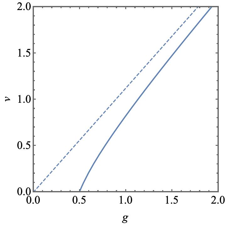
Figure 7: Plot of $v=V/(t+K)$ vs $g=J/3(t+K)$ predicted by equations (69) and (70). The dashed line gives the asymptotic large $g$ limit $\nu=(9/8)g$ of the phase boundary.

V Vicinity of the QCP

The vicinity to the quantum critical point at $g=g_{c}$, $\mu=0$ is of particular interest. Phase transitions in systems with Dirac spectrum lie in the class of of Gross-Neveu-Yukawa models [43]. Renormalization group analyses of this class of models indicate that the quantum critical point acquires full Lorentz invariance (which in mean-field theory corresponds to the case $t=K$). The corresponding long-wavelength action for our case is the deformation of Eq.(57):

$$H=\sum_{{\bf k}\in{\triangleleft}}\Psi\begin{pmatrix}-it(\vec{\alpha}\cdot\vec{\nabla})-\mu\tau_{3}&\vec{\sigma}{\cal V}\cr{\cal V}^{\dagger}\vec{\sigma}&it(\vec{\alpha}\cdot\vec{\nabla})\end{pmatrix}\Psi+$$

$$\frac{1}{2}{\cal V}^{+}(-\nabla^{2}+m^{2}){\cal V}+\lambda({\cal V}{\cal V}^{+})^{2}.$$ (71)

The survival of a relativistic majorana in the broken symmetry phase is rather striking consequence of the mismatch between the number of electron and majorana channels. These features may be of interest in the generalization of these ideas from quantum materials to exotic scenarios of broken symmetry in the vacuum.

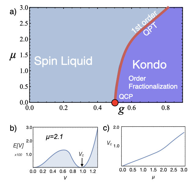
Figure 8: a) Mean field phase diagram as a function of chemical potential $\mu$. At $\mu=0$, the quantum phase transition from the spin liquid to the Kondo phase is a quantum critical point. b) representative plot of mean-field energy $E[V]$ versus $V$ illustrating first order minimum that develops at finite $\mu$. c) Critical value $V_{c}$ at first order quantum phase transition, showing that $V_{c}/\mu\sim 0.5$, corresponding to a direct transition into a state with a single neutral majorana cone of excitations. Calculations were made using $K=1,t=2$.

V.1 Finite doping $\mu\neq 0$

At finite doping, away from charge neutrality, the decoupled conduction sea develops a Fermi surface. In principle, the excitation spectrum of the condensate becomes more complex, for at $V=0^{+}$, there are three Fermi surfaces: two derived from the conduction electrons and one derived from the $\chi$ fermions. In principle, as the hybridization is increased from zero, the Fermi surfaces undergo a sequence of Lifschitz transitions, until entirely disappearing once $|V|\sim|\mu|/2$, they entirely vanish, entering the phase with a single neutral Majorana excitation cone, qualitatively identical to that obtained at $\mu=0$. (See Fig. 8.).

However, the mean-field theory predicts that these intermediate phases are entirely bypassed by a first order transition into the high $V$ state. This can be qualitatively understood from the dependence of the Ginzburg Landau free energy on $\mu$ and $V$, which in the vicinity of the $\mu=0$ QCP is given by

$$E=a\mu^{2}V+\tau V^{2}+bV^{3},$$ (72)

where $\tau\propto(g_{c}-g)$. The coefficients $a$ and $b$ depend on the ratio $t/K$,  and can be evaluated explicitly for the relativistic case $t/K=1$, confirming that they are both positive. The term linear in $V$ results from the development of a gap $V$ in the electron Dirac cones. Since the density of states is proportional to energy, in the normal state there is a Fermi surface containg $O(\mu^{2})$ electrons, giving rise to an increase in energy of order $\mu^{2}|V|$, so that $a>0$. This energy is reminiscent of the Van der Waals equation of state in the vicinity of the liquid-gas critical point, and gives rise to a first order phase transition at $\tau=-2|\mu|\sqrt{ab}$ into a state with $V_{c}=|\mu|\sqrt{\frac{a}{b}}$. Fig. 8 displays a detailed calculation of the mean-field free energy at finite doping, showing that at the crical $g$, a minimum in the free energy degenerate with the ground-state develops at finite $V_{c}\sim 0.5|\mu|$.

VI Fractionalized order

We now address the nature of the long-range order associated with the hybridization between electrons and Majorana fermions. Since the hybridization carries $Z_{2}$ gauge charge, the definition of long-range order requires the insertion of a gauge string. We can construct the following density matrix

$${\Sigma}_{ab}(x,y) = \langle\hat{\cal V}_{a}(x)\hat{\cal P}(x,y)\hat{\cal V}^{\dagger}_{b}({y})\rangle,$$ (73)

where $\hat{\cal P}(x,y)=\prod_{l}u_{(l+1,l)}$ is the string operator linking the sites $x$ and $y$ and ${\cal V}(x)$ is the four-component Kondo hybridization introduced in (54)

$$\hat{\cal V}(x)=\frac{1}{\sqrt{2}}\begin{pmatrix}v_{\uparrow}(x)\cr v_{\downarrow}(x)\cr-v^{\dagger}_{\downarrow}(x)\cr v^{\dagger}_{\uparrow}(x)\end{pmatrix}.$$ (74)

$\Sigma_{ab}(x,y)$ determines the amplitude for an electron to coherently tunnel through the spin liquid from $y$ to $x$.

Like the underlying gauge fields, the gauge strings $\hat{\cal P}(x,y)$ are constants of motion, commuting with the Hamiltonian and the constraints. The energetic cost of visons allows us to safely set all $u_{i_{A},j_{B}}=1$ in the ground-state, so the string variable is simply unity,

$$\hat{\cal P}(x,y)=1,\qquad\hbox{(axial gauge)},$$ (75)

and in this gauge, $\Sigma(x,y)$ reverts to a conventional two point functions. This is precisely the gauge we have used for the mean-field theory, so the mean-field density matrices factorize into a product of the spinors

$$\Sigma_{ab}(x,y)={\cal V}_{a}(x){\cal V}^{\dagger}_{b}(y).$$ (76)

Importantly, since this factorization occurs in a $Z_{2}$ gauge invariant quantity, it is true in all gauges, and is thus immune to the average over gauge orbits that annihilates gauge dependent quantities (the origin of Elitzur’s no-go theorem). Of course, mean-field theory is corrected by Gaussian fluctuations of the fields, but these $Z_{2}$ gauge invariant corrections are no different to the corrections that occur in conventional ODRLO, so we expect that beyond a coherence length, the factorization will be preserved as an asymptotic long-distance property, i.e

$$\langle{\cal V}({x})\hat{\cal P}(x,y){\cal V}^{\dagger}({y})\rangle\xrightarrow[]{|x-y|\rightarrow\infty}{\cal V}(x){\cal V}^{\dagger}(y).$$ (77)

This is the phenomenon of order fractionalization.

We can extract two interesting quantities from this density matrix, a $Z_{2}$ string-expectation value

$$Z(x,y)={\rm Tr}[\Sigma(y,x)]=\langle\hat{\cal V}^{\dagger}(x)\hat{\cal P}(x,y)\hat{\cal V}(y)\rangle,$$ (78)

and an $SO(3)$ matrix

$$D_{ab}(x,y) = {\rm Tr}[\Sigma(y,x)\sigma^{a}\tau^{b}]$$ (79)

$$= \langle\hat{\cal V}^{\dagger}(x)\sigma^{a}\tau^{b}\hat{\cal V}(y)\hat{\cal P}(x,y)\rangle,$$ (80)

The local density matrix $D_{ab}(x,x)=(2V^{2}/J)[\hat{d}^{b}(x)]_{a}$ determines the composite magnetism and pairing at site $x$, where the $(\hat{d}^{b})_{a}={\cal Z}^{\dagger}(x)\sigma^{a}\tau^{b}{\cal Z}(x)$ is the triad of local vectors introduced in (12) and we have normalized the spinors using (46) and (54). The composite order $D_{ab}(x,x)$ only determines the spinor-order up to a sign. However, the factorization of the scalar $Z(x,y)$

$$Z(x,y)\xrightarrow[]{|x-y|\rightarrow\infty}{\cal V}^{\dagger}(x){\cal V}(y)$$ (81)

is sensitive to the relative sign of the order parameter $v(x)$ at sites $x$ and $y$.

We can further emphasize the physical nature of these results by rewriting the order parameter and the gauge string in terms of variables from the original model. Using (8) and the constraint $-2i\Phi_{j}^{S}\Phi_{j}^{T}=1$(21) we can rewrite the hybridization field in terms of the composite operator ${\cal F}_{j}=(\vec{\sigma}\cdot\vec{S}_{j})c_{j}$, as

$$\hat{v}_{j}=(\vec{\sigma}\cdot\vec{\chi}_{j})c_{j}=2i\Phi^{T}_{j}{\cal F}_{j}.$$ (82)

By substituting $u_{(i,j)}=-2i\epsilon_{x_{i}x_{j}}b^{\alpha_{ij}}_{i}b^{\alpha_{ij}}_{j}$, where

$$\epsilon_{x^{\prime},x}\equiv\begin{pmatrix}1&1\cr-1&-1\end{pmatrix}=\left\{\begin{array}[]{cc}1&(x^{\prime}\in A)\cr-1&(x^{\prime}\in B)\end{array}\right.$$ (83)

into the string $\hat{\cal P}(x^{\prime},x)=\prod_{l}u_{(l+1,l)}$, then using the relation $\vec{\lambda_{j}}=-i\vec{b}_{j}\times\vec{b}_{j}$ (19) at the bond intersections and $b^{\alpha}_{j}=\Phi_{j}^{T}\lambda_{j}^{\alpha}$ (17) at its two ends, we can rewrite the string as $\hat{\cal P}=-2i\Phi^{T}_{x^{\prime}}\Phi^{T}_{x}{\cal P}^{\prime}$, where

$$\hat{\cal P}^{\prime}(x^{\prime},x)=s(x^{\prime},x)\prod_{j\in{\cal P}}\lambda_{j}^{a_{j}}$$ (84)

is a product of $\lambda$ operators taken along directions $a_{j}$ extremal to the path $\cal P$ (see Fig. 10), including an initial $\lambda^{a_{i}}_{i}$ and final $\lambda^{a_{f}}_{f}$ operator, oriented along the initial and final bonds. The parity $s(x^{\prime},x)=\pm 1$ is determined by the relative directions of the initial and final bond-vectors, $\hat{v}$ and $\hat{v}^{\prime}$

$$s(x^{\prime},x)=\left\{\begin{array}[]{cl}\epsilon_{x^{\prime},x},&(\hat{v}\cdot\hat{v}^{\prime}=0)\cr{\rm sgn}[(\hat{v}^{\prime}\times\hat{v})\cdot\hat{z}],&(\hat{v}\cdot\hat{v}^{\prime}\neq 0)\end{array}\right.$$ (85)

where $\hat{z}$ is normal to the plane.

In the ground-state, ${\cal P}$ does not depend on the path, so

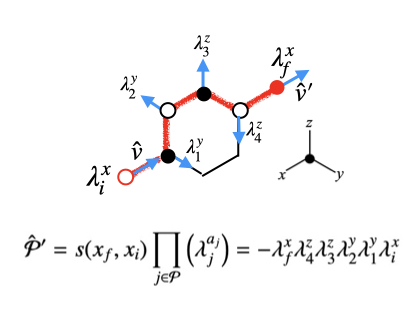
Figure 9: An example of the string operator ${\cal P}^{\prime}$ in Eq.(84).

$$-2i\langle{\cal F}_{a}(x){\cal F}^{\dagger}_{b}(y)\hat{\cal P}^{\prime}(x,y)\rangle\xrightarrow[]{|x-y|\rightarrow\infty}v_{a}(x)v^{\dagger}_{b}(y).$$ (86)

In other words, the composite fermions have developed a gauged off-diagonal long-range order. By (82), the composite fermions split up into a bosonic spinor with long range order, and an ancillary majorana that decouples from the Hilbert space:

$${\cal F}_{j}=(\vec{\sigma}\cdot\vec{S}_{j})c_{j}=-iv(x)\Phi^{T}(x).$$ (87)

This remarkable transmutation in the statistics of the composite fermions is a direct consequence of order fractionalization.

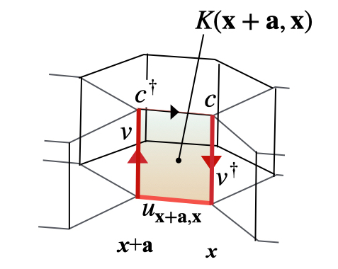
Figure 10: Kondo plaquet. The energetic cost of flux through the blue area favors a uniform arrangement of the spinor order parameter.

VI.1 Topology and Vison Confinement

The Yao Lee and Kitaev spin liquids have a topological degeneracy. We now discuss how this is modified by the presence of a Kondo hybridization. Suppose we have a domain across which the $Z_{2}$ string (78) $Z(x,y)$ changes sign. At the domain boundary, there is a “Kondo flux” identified with an inter-layer plaquette that links the conduction and spin fluids

$$K(x+{\bf a},x)=\langle c^{\dagger}(x+{\bf a})v(x+{\bf a})u_{x+{\bf a},x}v^{\dagger}(x)c(x)\rangle.$$ (88)

$K(x+{\bf a},x)$ describes the amplitude for an electron to traverse a rectangular path entering the spin liquid at $x$, exiting at $x+{\bf a}$ and returning via the conduction sea (see Fig 10). This favors a ground-state with a spinor $v(x)$ that is uniform in both direction and sign.

If we separate two visons without allowing the spinor background to deform, then we create a ladder of bonds with $u_{ij}=-1$. The reversed sign in the ladder then gives rise to a Kondo domain wall with cost $E(L)\propto L$ proportional to its length. In this situation, the visions would be linearly confined, and the cost of a $Z_{2}$ vortex through the torus would be proportional to the circumference of the torus, $E_{Z_{2}}\propto L_{C}$ (Fig. 12). This is the situation we would expect if the Kondo hybridization were a $Z_{2}$ scalar (a situation that would occur if the conduction band were made of three, rather than four majoranas, giving rise to an O(3), rather than an SU(2) Kondo model.)

However, the two visons can remove the domain wall by binding themselves to a “$2\pi$” or “$h/2e$” vortex in which the principle axes $\hat{d}^{b}$ rotate about some axis through $2\pi$. A $2\pi$ rotation of the spinor ${\cal V}(\theta)=e^{-i\frac{\theta}{2}\tau_{z}}{\cal V}_{0}$ causes it to pick up a minus sign: ${\cal V}(2\pi)=-{\cal V}_{0}$. In isolation, such a vortex would give rise to a sharp discontinuity in the spinor, but if the jump in ${\cal V}$ is located along the ladder where the gauge field $u_{ij}$ changes sign, then the Kondo domain is now removed and the gauged density matrix $\Sigma_{ab}(x,y)$ remains a smooth, single valued function. Since the energy cost of separating two vortices grows as $\ln L$, the resulting vortex-vison bound-state is logarithmically confined.

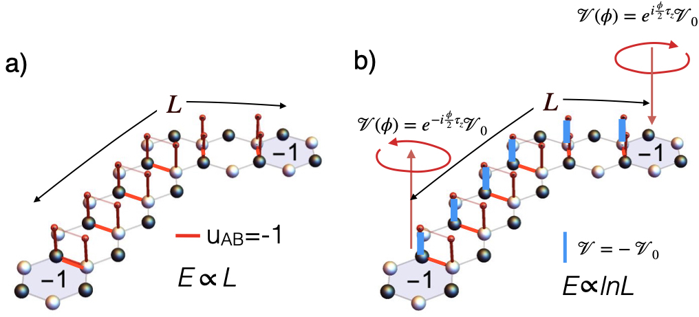
Figure 11: a) When two visons are separated a distance $L$, they introduce a ladder of $u_{ij}=-1$, giving rise to Kondo domain wall whose energy grows linearly with length $E(L)\propto L$. (b) If each vison bind to a “$2\pi$” vortex of the ${\cal V}$ field, the domain wall is eliminated, so the vison-vortex combination is logarithmically confined, with an energy $E(L)\propto\ln L$.

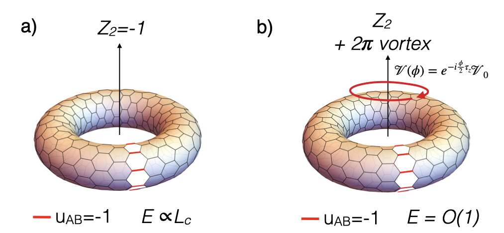
Figure 12: a) A $Z_{2}$ vortex through the torus is formed by a row of $u=-1$ bonds. In the Yao-Lee model, the domain wall costs no energy, but in the presence of a uniform order parameter $\cal V_{0}$, the domain wall costs an energy $E(L)\propto L_{C}$, where $L_{C}$ is the circumference of the torus. (b) When the $Z_{2}$ vortex binds a $2\pi$ vortex of the hybridization, the domain wall is removed, giving rise to an energy $E\sim O(1)$ which is intensive in the torus dimensions, restoring the single-valued character of the gauged off-diagonal long-range order.

In a similar fashion, if we create two visons, separating them and re-annihilate them after passing one around a ring of the torus, we create a $Z_{2}$ vortex through the torus, with a Kondo domain wall that passes right around it ( see Fig. 12a). This process costs no energy in a pure Kitaev or Yao Lee model, and is the origin of their topological degeneracy. Let us now consider the influence of the Kondo effect. In a model where the Kondo coupling were $Z_{2}$ scalar[44] as in the double layer Yao-Lee model with the Heisenberg exchange interaction between the layers, this would cost an energy proportional to the circumference $L_{C}$ of the torus. However, if we also introduce a vortex in which the ${\cal V}(x)$ rotates through $2\pi$, as shown on Fig. 12b, the spinor picks up an additional minus sign in passing around the vortex, and we then remove the discontinuity in the function $\Sigma_{ab}(x,y)$, removing the domain wall. This state with a combined $Z_{2}$ and $2\pi$ vortex only costs the energy to twist the spinor order through $\pi$, which involves an elastic energy $(\rho_{s}/2)(\pi/L)^{2}\times LL_{C}=\pi^{2}\rho_{s}/2(L_{C}/L)$, where $\rho$ is the stiffness, a value which is intensive in the linear size. Since this configuration cannot be smoothly returned to the original ground-state without creating a Kondo domain wall, the bound combination of a $2\pi$ vortice and vison pairs is topologically distinct excitation of the ground-state.

VII Triplet pairing condensate

VII.1 Electron self-energy

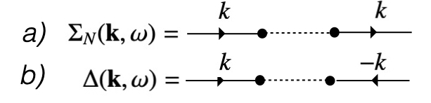
Figure 13: When an electron scatters through the spin liquid it can emerge a) as an electron, giving rise to resonant scattering and b) as a hole, giving rise to resonant Andreev reflection.

Once the spinor $\hat{v}_{j}$ condenses (dark blue region of Fig. 8), the resulting condensate will coherently scatter electrons through the spin liquid. The order fractionalization means that an electron can remain submerged within the spin liquid over arbitrarily long distances. When a Majorana spinon resurfaces into the electron fluid, it can do so as either a particle, or a hole, so the scattering amplitude of electrons via the spin liquid develops both normal and anomalous (Andreev) scattering components (Fig. 13). To examine these processes, consider the conduction electron self-energy that results from integrating out the majoranas $\chi_{{\bf k}}$. From (35), the propagator for the majoranas in the unhybridized spin liquid is

$$G^{(0)}_{\chi}({\bf k},\omega)=\frac{1}{\omega-{\vec{\gamma}_{s{\bf k}}}\cdot\vec{\alpha}}\ ,$$ (89)

where $\vec{{\gamma}_{{\bf k}}}=({\rm Re}\gamma_{{\bf k}},-{\rm Im}\gamma_{{\bf k}},0)$ and $\gamma_{s{\bf k}}=K\gamma_{{\bf k}}=iK(1+e^{i{\bf k}\cdot{\bf R}_{1}}+e^{i{\bf k}\cdot{\bf R}_{2}})$. Integrating out the majoranas in (57) then introduces a self-energy to the conduction electrons given by

$$\Sigma({\bf k},\omega) = \sigma^{a}{\cal V}G^{(0)}_{\chi}({\bf k},\omega){{\cal V}^{\dagger}}\sigma^{a}$$ (90)

$$= \sigma^{a}{\cal V}\frac{1}{\omega-\vec{\gamma}_{s{\bf k}}\cdot\vec{\alpha}}{{\cal V}^{\dagger}}\sigma^{a},$$ (91)

where we sum over the repeated index $a$.

By commuting the ${\cal V}={\rm V}{\cal Z}$ through the $\vec{\alpha}$, we obtain

$$\Sigma({\bf k},\omega)=\frac{{\rm V}^{2}}{\omega-\vec{\gamma}_{s{\bf k}}\cdot\vec{\alpha}}(\sigma^{a}{\cal Z}{\cal Z^{\dagger}}\sigma^{a}).$$ (92)

Using the identity ${\cal Z}{\cal Z}^{\dagger}+\sigma^{a}{\cal Z}{\cal Z}^{\dagger}\sigma^{a}=1$, we can then write the conduction self-energy in the form

$$\Sigma({\bf k},\omega)=\frac{\rm V^{2}}{\omega-\vec{\gamma}_{s{\bf k}}\cdot\vec{\alpha}}(1-{P}),$$ (93)

where ${P}={\cal Z}{\cal Z}^{\dagger}$ projects onto the zeroth Majorana component of the conduction sea, which consequently does not hybridize with the spin liquid. Without the projector ${P}$, this scattering would describe a Kondo insulator on a honeycomb lattice: the introduction of the projector breaks both time-reversal and gauge symmetry by eliminating a specific Majorana component of the conduction sea.

To examine the pairing components of the self-energy we write ${\cal Z}{\cal Z}^{\dagger}=\frac{1}{4}(1+d_{ab}\sigma^{a}\tau^{b})$ where the $d_{ab}\equiv({\bf d}^{b})_{a}={\cal Z}^{\dagger}\sigma^{a}\tau^{b}{\cal Z}$ are the triad of orthogonal vectors $({\bf d}^{1},{\bf d}^{2},{\bf d}^{3})$ that define the composite SO(3) order (see (12)). For the choice ${\cal Z}={\cal Z}_{0}=\frac{1}{\sqrt{2}}(1,0,0,1)^{T}$, the d-vectors align with the co-ordinate axes, $({\bf d}^{1},{\bf d}^{2},{\bf d}^{3})=({\bf x},{\bf y},{\bf z})$. The resonant scattering off the spin liquid takes the form

$$\Sigma({\bf k},\omega)={\rm V}^{2}\tfrac{1}{4}\left(3-({\bf d}^{b}\cdot\textpdfrender{TextRenderingMode=FillStroke,LineWidth=.35pt,}{\sigma})\tau^{b}\right)\frac{\omega+\vec{\gamma}_{s{\bf k}}\cdot\vec{\alpha}}{\omega^{2}-|\gamma_{s{\bf k}}|^{2}}.$$ (94)

We can divide the self-energy into normal and pairing components

$$\Sigma=\Sigma_{N}+\Delta({\bf k},\omega)\tau_{+}+\Delta^{\dagger}({\bf k},\omega)\tau_{-},$$ (95)

where

$$\Sigma_{N}({\bf k},\omega) = \tfrac{1}{4}\left(3-({\bf d}^{3}\cdot\textpdfrender{TextRenderingMode=FillStroke,LineWidth=.35pt,}{\sigma})\tau_{3}\right)\Sigma_{0}({\bf k},\omega),$$ (96)

$$\Delta({{\bf k},\omega}) = -\tfrac{1}{4}\left(({\bf d}^{1}+i{\bf d}^{2})\cdot\textpdfrender{TextRenderingMode=FillStroke,LineWidth=.35pt,}{\sigma}\right)\Sigma_{0}({\bf k},\omega).$$ (97)

Here,

$$\Sigma_{0}={{\rm V}}^{2}\left(\frac{\omega+\vec{\gamma}_{s{\bf k}}\cdot\vec{\alpha}}{\omega^{2}-|\gamma_{s{\bf k}}|^{2}}\right).$$ (98)

$\Sigma_{N}$ describes a kind of odd-frequency magnetism (with no onsite magnetic polarization). The second-term $\Delta({\bf k},\omega)$ in (96) describes a triplet gap function, with a complex d-vector $\hat{\bf d}^{1}+i{\bf d}^{2}$ which breaks time-reversal symmetry.

The frequency, momentum and sublattice structure of the pairing is an interesting illustration of the SPOT=-1[45] acronym for the exchange-antisymmetry of pairing, where S, P, O and T are the parities of the pairing under spin exchange, spatial inversion, sublattice exchange and time inversion, respectively. Here, since the pairing is triplet and spin symmetric (S=1), POT=-1: there are in fact three separate odd-frequency, odd-parity and odd-sublattice components. The term proportional to $\omega$ is odd frequency, (T=-1, P=O=+1), while the even-frequency component (T=+1) divides into two parts $\vec{\gamma}_{s{\bf k}}\cdot\vec{\alpha}=(\gamma^{1}_{s{\bf k}}\alpha_{1}+\gamma^{2}_{s{\bf k}}\alpha_{2})$ which are respectively, odd parity, sublattice even (P=-1, O=+1) and even parity, sublattice odd (P=+1, O=-1).

VII.2 Long-range tunneling

The structure of the self-energy reflects the long-range tunneling of electrons through the spin liquid. If the order parameter ${\cal V}(x)$ varies slowly in space and time, the electron self-energy takes the form

$$\Sigma(x,x^{\prime})=\sigma^{a}{\cal V}(x){\cal G}(x-x^{\prime}){\cal V}^{\dagger}(x^{\prime})\sigma^{a}$$ (99)

where

$${\cal G}(x-x^{\prime})=\int\frac{{}d^{3}k}{(2\pi)^{3}}\left(\frac{1}{\omega-\gamma_{s{\bf k}}\cdot\vec{\alpha}}\right)e^{i({\bf k}\cdot{\bf x}-\omega t)}$$ (100)

is the majorana propagator for the spin liquid. At long distances, this propagator is dominated by the relativistic structure of the excitations around the Dirac point at ${\bf K}$, where $\gamma_{s{\bf k}+{\bf K}}=ic(k_{x}+ik_{y})$ ($c=3K/2$ ). The approximate structure of $\Sigma(x,x^{\prime})$ can be obtained by power-counting: since ${\cal G}(k)\sim 1/k$ in Fourier space, ${\cal G}(x)\sim 1/x^{2}$, so we expect that

$$\Sigma(x,x^{\prime})\sim\left[\sigma^{a}{\cal V}(x)\frac{1}{|x-x^{\prime}|^{2}}{\cal V}^{\dagger}(x^{\prime})\sigma^{a}\right]e^{i{\bf K}\cdot({\bf x}-{\bf x}^{\prime})}$$ (101)

where $|x|^{2}=x^{2}-c^{2}t^{2}$. A more detailed calculation gives

$${\cal G}(\vec{x},t)=\frac{ct-\vec{x}\cdot\vec{\beta}}{4\pi|x|^{3}}e^{i{\bf K}\cdot{\bf x}}$$ (102)

where $\vec{\beta}=(\alpha_{y},\alpha_{x})$ defines the sublattice structure of the tunneling.

This infinite-range, power-law decay of the tunneling amplitude means that in the ground-state, the tunneling electrons sample the fractionalized order at arbitrarily large distances. In this way, we see that the development of a decoupled, coherent, neutral Dirac cone is a direct consequence of the fractionalization of the order at infinite length scales.

VIII Statistical Mechanics and Long Wavelength action

VIII.1 Statistical Mechanics and Phase Diagram

We now discuss the statistical mechanics and long-wavelength of the order fractionalized phase.

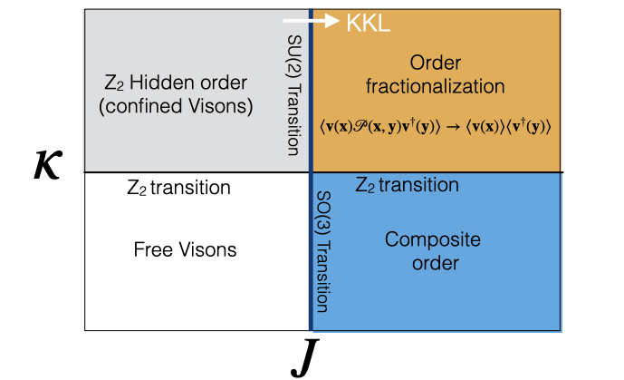
Figure 14: Schematic Phase diagram for the 3D classical gauged spinor model from (103). White arrow shows the order-fractionalization transition.

When we integrate out the Fermions from the model, we are left with a $Z_{2}$ lattice gauge theory of the spin liquid, coupled to the “matter fields” provided by the Kondo spinors $v_{j}$

$$H=-J\sum_{(i,j)}v^{\dagger}_{i}u_{ij}v_{j}+U\sum_{j}(v^{\dagger}_{j}v_{j}-1)^{2}-\kappa\sum_{p}\prod_{\square}u_{(l,m)}.$$ (103)

where the the $U$ term constrains the $v_{j}$ to fixed magnitude and final plaquette term ascribes an energy cost of $2\kappa$ to each vison. Here we have used our earlier notation $u_{(l,m)}$ where the parentheses orders the site indices so that the $A$ sublattice is first. The condensed $v$-spinors are the Higgs fields for the $Z_{2}$ gauge field $u$, transforming its uncontractible Wilson loops into “Kondo domain walls” of finite energy density. (Fig. 12) At finite temperatures, we expect no phase transitions, for the orientational degrees of freedom are eliminated by the Mermin Wagner theorem, and the presence of small but finite concentrations of visons eliminates the possibility of a $Z_{2}$ phase transition .

There is an interesting issue to what extent charge $e$ bosons may survive as excitations at nonzero $T$. This depends on the ratio of $J$ to the vison gap of order $\kappa$. Consider the average of a large Wilson loop of area $S$. Its value for a configuration with $n$ visons is $(-1)^{n}$. At $J_{K}=0$ the gauge field is not higgsed, the excitations are point-like visons. The probability of such a configuration is $\sim C_{S}^{n}\exp[-n\kappa/T]$, where $C_{S}^{n}=n!(S-n)!/S!$ is a combinatoric pre-factor. The sum over configurations gives

$$\langle W(S)\rangle=\sum_{n}(-1)^{n}C^{n}_{S}=(1-\exp[-\kappa/T])^{S}=e^{-S/\pi R^{2}}$$ (104)

giving rise to an area-law confinement at finite T with a confinement area $\pi R^{2}\sim 1/{\ln(1-e^{-\kappa/T})}\sim e^{\kappa/T}$ proportional to the inverse vison density. On the other hand the correlation length $\xi$ of the $v({\bf x})$-fields calculated in the limit $\kappa\rightarrow\infty$ is $\xi\sim\exp(J/T)$. So, if $J{{\lower 4.0pt\hbox{$<$}}\atop\widetilde{\ \ \ }}\kappa$, then $\xi\ll R$ and finite-temperature confinement effects are superceded by the finite orientational correlation length of the order parameter and are thus unimportant.

However, the quantum model for the Kitaev Kondo lattice at zero temperature is equivalent to the statistical mechanics of the above $Z_{2}$ gauged spinor lattice in 3D [47]. In the absence of the matter fields, the pure 3D $Z_{2}$ lattice gauge theory develops an Ising phase transition for sufficiently large $\kappa$, into a phase where visons are absent[48]. At small finite $J$ the Ising transition persists, even though the orientational order of the spinors will be absent, corresponding to an entry into the Higg’s phase of the gauged Ising model. This phase corresponds to the Yao Lee model at zero temperature. (Grey region of Fig. 14). At still larger $J$, the $\hat{v}$ will develop orientational order in which $\Sigma_{ab}(x,y)\sim{\cal V}(x){\cal V}^{\dagger}(y)$ factorizes at long distances, corresponding to a state of fractionalized order. This is the phase transition described by our mean-field theory (Orange region of Fig. 14). Lastly, we note that in the region of large $J$, but small $\kappa$, (which is not applicable to the Kitaev Kondo model), the local quantity $\Sigma_{ab}(x,x)$ is expected to develop long range order in the presence of deconfined visons, corresponding to unfractionalized, vector order. In this phase, the order parameter is the unfractionalized composite order parameter (12). (Blue region of Fig. 14). The conjectured phase diagram for the model is shown in Fig. 14.

VIII.2 Long Wavelength action

A discussion of the long-wavelength action of the order fractionalized phase is simplified by taking the special case, where $K=t$, leading to a relativistic field theory with an effective speed of light $c_{E}=(3/2)K$ governing all excitations (see (V)). So long as there are no domain walls, the relativistic, coarse-grained action for slow variations in the spinor ${v}({\bf x},\tau)$ is

$$S={\rho_{s}}\int d^{2}xd\tau\left|\left(\partial_{\mu}+i\frac{e}{\hbar}A_{\mu}\right){v({\bf x})}\right|^{2}$$ (105)

where $\partial_{\mu}=(1/c_{E}\partial_{\tau},\vec{\nabla})$. It is convenient to rewrite this in terms of the four-component spinor ${\cal Z}$, as

$$S={\rho_{s}}\int d^{2}xd\tau\left|\left(\partial_{\mu}+i\frac{e}{\hbar}A_{\mu}\tau_{3}\right){\cal Z}\right|^{2}$$ (106)

If we write ${\cal Z}$ in terms of Euler angles,

$${\cal Z}=\exp\left[-i\frac{\phi}{2}\tau_{3}\right]\exp\left[-i\frac{\theta}{2}\tau_{2}\right]\exp\left[-i\frac{\psi}{2}\tau_{3}\right]\cal Z_{0},$$ (107)

then $\partial_{\mu}{\cal Z}=-\frac{i}{2}({\omega^{a}})_{\mu}\sigma_{a}{\cal Z}$ defines the components of the angular velocity $\vec{\omega}_{\mu}={\omega^{a}}_{\mu}{\bf d}^{a}$ measured in the body-axis frame, i.e $\partial_{\mu}{\bf d}^{b}=\vec{\omega}_{\mu}\times{\bf d}^{b}$. It follows that

$$\left(i\partial_{\mu}-\frac{e}{\hbar}A_{\mu}\tau_{3}\right){\cal Z}=\frac{1}{2}(\omega_{\mu}^{a}-\frac{2e}{\hbar}A_{\mu}\delta^{a3})\tau_{a}{\cal Z},$$ (108)

allowing us to rewrite the long-wavelength action in the the form of a principle chiral action,

$$S=\frac{\rho_{s}}{2}\int d^{2}xd\tau\left[(\partial_{\mu}\hat{n})^{2}+(\omega_{\mu}^{3}-\frac{2e}{\hbar}A_{\mu})^{2}\right]$$ (109)

where we have made the substitution $(\omega^{1}_{\mu})^{2}+(\omega^{2}_{\mu})^{2}=(\partial_{\mu}\hat{n})^{2}$ and $\hat{n}\equiv{\bf d}^{3}={\cal Z}^{\dagger}\vec{\sigma}\tau_{3}{\cal Z}$.

The action (109) resembles the action of a superconductor. However, there are a number of important differences.

• In contrast to a superconductor,

  $$J_{\mu} = -\frac{\delta S}{\delta A^{\mu}}=\frac{2e\rho_{s}}{\hbar}(\omega_{\mu}^{3}-\frac{2e}{\hbar}A_{\mu})$$ (110)

  $$= \frac{2e\rho_{s}}{\hbar}(\partial_{\mu}\psi-\frac{2e}{\hbar}A_{\mu}+\cos\theta\partial_{\mu}\phi)$$ (111)

  contains an additional term $\cos\theta\partial_{\mu}\phi$, derived from rotations of $\hat{n}$, so the magnetic aspects of the phase associated with $\hat{n}$ are intertwined with the superconducting properties.

• The first homotopy class $\pi_{1}(SU(2))=0$ is empty, implying that there are no topologically stable vortices of an SU(2) order parameter. Thus in general, any current loop can be relaxed by relaxed by the rotation of the magnetic vector $\hat{n}$ out of the plane. Magnetic anisotropy is required to stabilize superfuid or superconducting behavior[23].

• Although the vorticity of a screening current has no topological protection, for the case of charged conduction electrons, a fragile Meissner phase is expected[49], because the relaxation of surface screening currents requires the passage of skyrmions into the condensate. The energy of a single skyrmion is $4\pi\rho_{s}$, so their penetration into the bulk needs to offset by a finite field external field. Thus we expect that below a critical field, this paired state will exhibit a fragile Meissner effect[27].

Finally we note that a magnetic field introduces a Zeeman coupling to the electrons and the underlying spin liquid. The Yao-Lee spin liquid now acquires a Fermi surface. The effective action now contains terms of the form $-g\mu_{B}v^{\dagger}\sigma_{z}v$, which convert the physics into that of an $x-y$ model with a finite temperature BKT transition associated with the binding of vortices. One of the interesting questions, is whether this state will exhibit $h/e$ vortices characteristic of a charge $e$ condensate? In fact, the development of these vortices depends subtlely on the energetics of the visons[7]. The composite order parameter

$$\langle v^{T}({\bf x})i\sigma_{2}\vec{\sigma}v({\bf x})\rangle\sim(\hat{d}_{1}({\bf x})+id_{2}({\bf x}))$$ (112)

carries charge $2e$. If we rotate the vectors $d_{1}(x)$ and $\hat{d}_{2}(x)$ through $2\pi$ about the $\hat{d}_{3}(x)$ axis, we create an $h/2e$ vortex. Such a vortex rotates the underlying spinor order through $2\pi$, causing it to pick up a minus sign, so that two $h/2e$ vortices are connected by a Kondo domain wall whose energy grows with length, which would a priori bind two $h/2e$ vortices into a single $h/e$ vortex. However, the naked domain wall can be removed by binding a vison to the the $h/2e$ vortex. The confinement of the $h/2e$ vortices into $h/e$ vortices thus depends on whether the binding energy is negative, or

$$E\biggl{[}\frac{h}{e}\biggr{]}-2\left(E\biggl{[}\frac{h}{2e}\biggr{]}+E_{V}\right)<0$$ (113)

For small enough superfluid stiffness, this quantity is necessarily negative, so that in the vicinity of the quantum phase transition into the order-fractionalized state, we expect $h/e$ vortices to be stable in the fractionalized condensate.

IX Discussion: Broader Implications

We have presented a model realization of order fractionalization in a Kondo lattice where conduction electrons interact with a $Z_{2}$ spin liquid. Our theory, which describes the interaction of an emergent Z₂ gauge theory with matter, has several distinct features:

1. The order parameter, a spinor, carries charge $e$ and spin S=1/2.

2. The broken symmetry state has a gapless Majorana mode in the bulk, which results from a mismatch between the quantum numbers of the conduction electrons, which carry spin 1/2, charge $e$, and the elementary spin-one majorana excitations of the $Z_{2}$ spin liquid. This mismatch determines the quantum numbers of the order parameter formed as a bound-state between conduction electrons and Majorana fermions.

3. Fractionalized order, in which the spinor order parameter develops long-range order, allows the electrons to coherently tunnel through the spin liquid over arbitrarily long distances.

The condensation of an order parameter carrying a Z₂ charge is a direct consequence of the massive $Z_{2}$ gauge field, which eliminates visons and gives rise to deconfined Majorana fermions in the spin liquid. Although the models we have discussed, involve a static Z₂ gauge field, whose excitations - visons, are immobile, the phenomena we observe in our model only requires that the underlying spin-liquid contains gapped gauge excitations.

Some features of our model are related to its low dimensionality. In 2D fractionalized order is only strictly present at zero temperature when there are no visons, however, as we discussed in Section VIII.1, vestiges of order fractionalization order will persist to finite temperatures provided the correlation length $\xi$ of the order parameter is shorter than the confinement radius $R$ of the gauge field determined by the density of thermally excited visons. Order fractionalization is likely to become more robust in higher dimensions. In particular, like the Kitaev spin liquid, our model serves as a platform for an entire family of three dimensional lattices with trivalent co-ordination[50], including the hyperoctagonal lattice (the subject of a forthcoming paper [51]) where the phase transition occurs at finite temperature and at arbitrary small $J_{K}$ so that all analytical calculations can be performed in a controllable manner.

More generally, we expect that the order fractionalization observed in our model constitutes an emergent phenomenon with physically observable consequences in the quantum universe at large, including quantum materials, and in the context of relativistic theories (see section V). This wider context also includes the expectation of superconducting phases with gapless Majorana Fermi surfaces, and $Z_{2}$ phase transitions in which the domain walls associated with an emergent spinor order may manifest themselves as hidden order phase transitions. Several aspects of quantum materials, including heavy fermion compounds with hidden order, such as URu₂Si₂[52], and superconductors and insulators with signs of an underlying Fermi surface, such as UTe₂[53] and SmB₆[54] are interesting candidates for these novel possibilities.

Acknowledgements

This work was supported by Office of Basic Energy Sciences, Material Sciences and Engineering Division, U.S. Department of Energy (DOE) under Contracts No. DE-SC0012704 (AMT) and DE-FG02-99ER45790 (PC). AMT and PC contributed equally to this work. AMT is grateful to Lukas Janssen for an excellent presentation of their results on the YLK model and to Joerg Schmalian to valuable remarks. PC acknowledges discussions with Tom Banks, Premi Chandra, Eduardo Fradkin, Yashar Komijani and Subir Sachdev, and the support of the Aspen Center for Physics under NSF Grant PHY-1607611, where part of this work was completed.

Appendix A Alternative Fermionization of the Yao-Lee model using Jordan-Wigner Fermions

Like the Kitaev honeycomb model, the Yao-Lee model can be solved using a Jordan-Wigner transformation. This alternative fermionization scheme allows a derivation of the model that does not involve an expansion of the Hilbert space. The derivation here is an adaptation of that of Feng, Zhang and Xiang[55] for the Kitaev honeycomb model, that incorporates the additional degrees of freedom in Yao-Lee model. To see how this works, we first redraw the honeycomb as a brick-wall lattice, composed of one dimensional chains with alternating cross-links (see Fig. 15 A.), where the horizontal chains are labelled by the index $l$ , and the position along the chains is labelled by the index $j$. The Yao-Lee Hamiltonian with antiferromagnetic bond-strengths $K^{x}$, $K^{y}$ and $K^{z}$ is written

$$H=\frac{1}{2}\sum_{l+j\in\hbox{even}}\biggl{[}K^{x}(\lambda_{jl}^{x}\lambda_{j-1,l}^{x})\vec{\sigma}_{jl}\cdot\vec{\sigma}_{j-1,l}+K^{y}(\lambda_{jl}^{y}\lambda_{j+1,l}^{y})\vec{\sigma}_{jl}\cdot\vec{\sigma}_{j+1,l}+K^{z}(\lambda_{jl}^{z}\lambda_{j,l+1}^{z})\vec{\sigma}_{jl}\cdot\vec{\sigma}_{j,l+1}\biggr{]},$$ (114)

where the $\vec{\lambda}_{jl}$ and $\vec{\sigma}_{jl}$ are Pauli matrices for the orbital, and spin degrees of freedom, respectively. We label the sites so that $A$ sublattice $j+l$ is odd, while on the $B$ sublattice, $j+l$ is even.

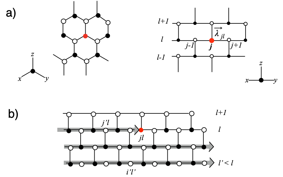
Figure 15: a) Equivalence between honeycomb and “brick-wall” lattice. “A” sites (white circles) correspond to odd $j+l$, whereas “B” sites (black circles) correspond to even $j+l$. b) Showing Jordan-Wigner string ${\cal P}_{jl}=\exp[i\Phi_{jl}]$ snaking along the rows up to site $(j,l)$.

Following [55], we carry out a Jordan-Wigner transformation on the frustrated orbital degrees of freedom $\lambda^{a}_{jl}$, as follows:

$$\lambda_{jl}^{+} = (\lambda_{jl}^{x}+i\lambda_{jl}^{y})/2=f^{\dagger}_{jl}{P}_{jl}$$ (115)

$$\lambda_{jl}^{-} = (\lambda_{jl}^{x}-i\lambda_{jl}^{y})/2=f_{jl}{P}_{jl}$$ (116)

$$\lambda_{jl}^{z} = 2n_{jl}-1,$$ (117)

where ${P}_{jl}=\exp[i\Phi_{jl}]$ is a real, $Z_{2}$ string operator, where

$$\Phi_{jl}=\pi\sum_{j^{\prime}<j}n_{j^{\prime}l}+\pi\sum_{i}\sum_{l^{\prime}<l,}n_{il^{\prime}}.$$ (118)

The string operator ${P}_{jl}$ runs from left to right along each row of the lattice, starting at the bottom left-hand corner, continuing until it reaches site $(j,l)$ (see Fig. 15 B. ) ${P}_{jl}$ commutes with the fermions $f_{mn}$ at sites above or to the right of site $(j,l)$, but anticommutes with all fermions $f_{mn}$ along its path, i.e sites to the left of $jl$ on the same row, and sites on any row below row $l$. This guarantees the the orbital operators $\lambda^{a}_{jl}$ commute between sites. Applying the Jordan-Wigner transformation to the orbital interaction terms in (114), we have

$$\lambda^{x}_{jl}\lambda^{x}_{j-1,l} = (f_{j,l}+f^{\dagger}_{j,l})(f_{j-1,l}-f^{\dagger}_{j-1,l}),$$ (119)

$$\lambda^{y}_{j+1,l}\lambda^{y}_{j,l} = (f^{\dagger}_{j+1,l}-f_{j+1,l})(f^{\dagger}_{j,l}+f_{j,l}),$$ (120)

$$\lambda^{z}_{jl}\lambda^{z}_{j,l+1} = (2n_{jl}-1)(2n_{j,l+1}-1),$$ (121)

so that the fermionized Hamiltonian becomes

$$H = \frac{1}{2}\sum_{l+j\in\hbox{even}}\biggl{[}K^{x}(f_{jl}+f_{jl}^{\dagger})(f_{j-1l}-f^{\dagger}_{j-1l})(\vec{\sigma}_{jl}\cdot\vec{\sigma}_{j-1l})$$ (122)

$$+ K^{y}(f^{\dagger}_{j+1l}-f_{j+1l})(f^{\dagger}_{jl}+f_{jl})(\vec{\sigma}_{jl}\cdot\vec{\sigma}_{j+1l})$$ (123)

$$+ K^{z}(2n_{jl}-1)(2n_{j,l+1}-1)(\vec{\sigma}_{jl}\cdot\vec{\sigma}_{jl+1})\biggr{]}.$$ (124)

Splitting the fermions into their Majorana components, choosing $f_{jl}=(c_{jl}{\color[rgb]{1,0,0}-}ib_{jl})/\sqrt{2}$ for even $j+l$, while $f_{jl}=(b_{jl}+ic_{jl})/\sqrt{2}$ for odd $j+1$, so that $c_{jl}=(f_{jl}+f^{\dagger}_{jl})/\sqrt{2}$ (even $j+l$) and $c_{j,l}=i(f_{j,l}-f^{\dagger}_{j,l})/\sqrt{2}$ (odd $j+l$) and

$$(2n_{jl}-1)(2n_{j,l+1}^{z}-1)=ic_{j,l+1}u_{jl+1,jl}c_{jl},$$ (125)

where $u_{jl+1,jl}={\color[rgb]{1,0,0}-}2ib_{jl+1}b_{jl}$ is a $Z_{2}$ field operator with eigenvalues $\pm 1$ that lives on the vertical $z$ bonds. The Hamiltonian can then be written

$$H = \sum_{j+l\in\hbox{even}}i(K^{x}c_{j-1l}\vec{\sigma}_{j-1l}+K^{y}c_{j+1l}\vec{\sigma}_{j+1l}$$ (126)

$$+ K^{z}c_{jl+1}\vec{\sigma}_{jl+1}u_{jl+1,jl})\cdot c_{jl}\vec{\sigma}_{jl}.$$ (127)

Notice that the operators $u_{jl+1,jl}=-2ib_{j,l+1}b_{j,l}$ only appear on vertical bonds in the Hamiltonian, commuting with the entire Hamiltonian, forming static $Z_{2}$ gauge fields.

Finally, we note that the operators

$$\vec{\chi}_{jl}=c_{jl}\vec{\sigma}_{jl}$$ (128)

are real, and satisfy canonical anticommutation relations

$$\chi^{a}_{jl}=(\chi^{a}_{jl})^{\dagger},\qquad\{\chi^{a}_{jl},\chi^{b}_{mn}\}=\delta^{ab}\delta_{jm}\delta_{ln},$$ (129)

enabling us to identify them as independent Majorana fermions (normalized so that $(\chi^{a}_{jl})^{2}=1/2$). The Hamiltonian thus reverts to the fermionized version of the Yao-Lee model

$$H=\sum_{\langle i,j\rangle}iK^{\alpha_{ij}}u_{i,j}(\vec{\chi}_{i}\cdot\vec{\chi}_{j})$$ (130)

in the gauge where the gauge fields $u^{x}_{(i,j)}=u^{y}_{(i,j)}=1$ are set to unity in the $x$ and $y$ directions. With this gauge choice the flux through each hexagon is determined by the vertical bonds alone. (In our treatment of the model, we set all $K^{a}=K$ to be equal.)

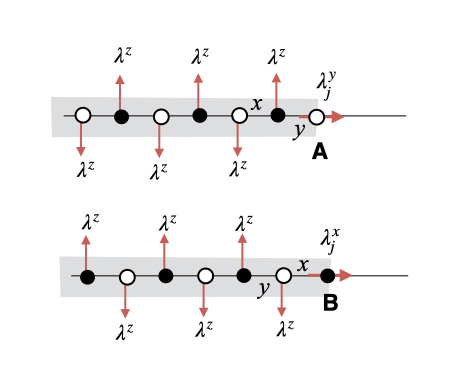
Figure 16: The modified string operator ${\cal P}_{j}$ incorporates the final link on the string as an extremal bond.

Lastly, note that we can invert the Jordan-Wigner transformation, identifying

$${P}_{jl}=\prod_{j^{\prime}l^{\prime}\in P}\lambda^{z}_{j^{\prime}l^{\prime}}$$ (131)

as the product of the orbital matrices along the path $P$ of the string (not including site $(j,l)$ ). The $\chi$ majoranas can then be written as

$$\frac{1}{\sqrt{2}}\vec{\chi}_{jl}=\vec{S}_{jl}{P}_{jl}\times\left\{\begin{array}[]{cc}\lambda^{y}_{jl},&(\hbox{A site}\ j+l\in\hbox{odd}),\cr\lambda^{x}_{jl},&(\hbox{B site}\ j+l\in\hbox{even}),\end{array}\right.$$ (132)

We can incorporate the dangling $\lambda^{a}$ operators by regarding the final link on the string as an extremal bond, defining

$${\cal P}_{jl}=\lambda_{jl}^{\alpha_{jl,j-1l}}P_{jl}$$ (133)

so that now

$$\frac{1}{\sqrt{2}}\vec{\chi}_{jl}=\vec{S}_{jl}{\cal P}_{jl}$$ (134)

providing a unique, non-local expression for the Majorana spin excitations.

References

- Hansson et al. [2004] T. Hansson, V. Oganesyan, and S. Sondhi, Superconductors are topologically ordered, Annals of Physics 313, 497–538 (2004).
- Dirac [1955] P. A. M. Dirac, Gauge-invariant formulation of quantum electrodynamics, Canadian Journal of Physics 33, 55 (1955).
- Baskaran et al. [1987] G. Baskaran, Z. Zou, and P. W. Anderson, The resonating valence bond state and high-Tc superconductivity — A mean field theory, Sol. State Comm. 63, 973 (1987).
- Ioffe and Larkin [1989] L. B. Ioffe and A. I. Larkin, Gapless fermions and gauge fields in dielectrics, Phys. Rev. B 39, 8988 (1989).
- Ioffe and Kotliar [1990] L. B. Ioffe and G. Kotliar, Transport phenomena near the mott transition, Phys. Rev. B 42, 10348 (1990).
- Wen and Zee [1989] X. G. Wen and A. Zee, Effective theory of the t- and p-breaking superconducting state, Phys. Rev. Lett. 62, 2873 (1989).
- Sachdev [1992] S. Sachdev, Stable hc/e vortices in a gauge theory of superconductivity in strongly correlated system, Phys. Rev. B 45, 389 (1992).
- Balents et al. [2000] L. Balents, M. P. A. Fisher, and C. Nayak, Dual vortex theory of strongly interacting electrons: A non-fermi liquid with a twist, Phys. Rev. B 61, 6307 (2000).
- Senthil and Fisher [2000] T. Senthil and M. P. A. Fisher, gauge theory of electron fractionalization in strongly correlated systems, Phys. Rev. B 62, 7850 (2000).
- Komijani et al. [2018] Y. Komijani, A. Toth, P. Chandra, and P. Coleman, Order fractionalization (2018), arXiv:1811.11115 .
- Kasuya [1956] T. Kasuya, A Theory of Metallic Ferro- and Antiferromagnetism on Zener’s Model, Progress of Theoretical Physics 16, 45 (1956).
- Mott [1974] N. Mott, Rare-earth compounds with mixed valencies, Philosophical Magazine 30, 403 (1974).
- Doniach [1977] S. Doniach, Kondo lattice and weak antiferromagnetism, Physica B+C 91, 231 (1977).
- Read and Newns [1983] N. Read and D. M. Newns, On the Solution of the Coqblin-Schreiffer Hamiltonian by the Large-N Expansion Technique, Journal of Physics C: Solid State Physics 16, 3273 (1983).
- Coleman [1983] P. Coleman, expansion for the Kondo lattice, Phys. Rev. B 28, 5255 (1983).
- Auerbach and Levin [1986] A. Auerbach and K. Levin, Kondo Bosons and the Kondo Lattice: Microscopic Basis for the Heavy Fermi Liquid, Physical Review Letters 57, 877 (1986).
- Coleman and Andrei [1989] P. Coleman and N. Andrei, Kondo-stabilised spin liquids and heavy fermion superconductivity, J. Cond. Matt. 1, 4057 (1989).
- Senthil et al. [2003] T. Senthil, S. Sachdev, and M. Vojta, Fractionalized Fermi Liquids, Physical Review Letters 90, 216403 (2003).
- Coleman [1987] P. Coleman, Constrained quasiparticles and conduction in heavy-fermion systems, Phys. Rev. Lett. 59, 1026 (1987).
- Coleman et al. [2005] P. Coleman, J. B. Marston, and A. J. Schofield, Transport anomalies in a simplified model for a heavy-electron quantum critical point, Physical Review B 72, 245111 (2005).
- Oshikawa [2000] M. Oshikawa, Topological Approach to Luttinger’s Theorem and the Fermi Surface of a Kondo Lattice, Physical Review Letters 84, 3370 (2000).
- Hazra and Coleman [2021] T. Hazra and P. Coleman, Luttinger sum rules and spin fractionalization in the SU() Kondo lattice, Phys. Rev. Research 3, 033284 (2021).
- Coleman et al. [1994] P. Coleman, E. Miranda, and A. Tsvelik, Odd-frequency pairing in the Kondo lattice., Physical review B, Condensed matter 49, 8955 (1994).
- Coleman et al. [1993] P. Coleman, E. Miranda, and A. Tsvelik, Are Kondo insulators gapless?, Physica B: Condensed Matter 186-188, 362 (1993).
- Note [1] Note that throughout this paper, following contemporary physics usage, we shall use the term majorana as a proper noun to describe a Majorana fermion, thus using a lower-case “m”.
- Baskaran [2015] G. Baskaran, Majorana Fermi Sea in Insulating SmB6: A proposal and a Theory of Quantum Oscillations in Kondo Insulators, ArXiv e-prints (2015), arXiv:1507.03477 .
- Erten et al. [2017] O. Erten, P.-Y. Chang, P. Coleman, and A. M. Tsvelik, Skyrme insulators: Insulators at the brink of superconductivity, Phys. Rev. Lett. 119, 057603 (2017).
- Kitaev [2006] A. Kitaev, Anyons in an exactly solved model and beyond, Annals of Physics 321, 2 (2006).
- Yao and Lee [2011] H. Yao and D.-H. Lee, Fermionic magnons, non-abelian spinons, and the spin quantum Hall effect from an exactly solvable spin- Kitaev model with su(2) symmetry, Phys. Rev. Lett. 107, 087205 (2011).
- Yao et al. [2009] H. Yao, S.-C. Zhang, and S. A. Kivelson, Algebraic spin liquid in an exactly solvable spin model, Phys. Rev. Lett. 102, 217202 (2009).
- Wu et al. [2009] C. Wu, D. Arovas, and H.-H. Hung, -matrix generalization of the Kitaev model, Phys. Rev. B 79, 134427 (2009).
- Seifert et al. [2018] U. F. P. Seifert, T. Meng, and M. Vojta, Fractionalized Fermi liquids and exotic superconductivity in the Kitaev-Kondo lattice, Physical Review B 97, 085118 (2018), 1710.09381 .
- Seifert et al. [2020] U. F. P. Seifert, X.-Y. Dong, S. Chulliparambil, M. Vojta, H.-H. Tu, and L. Janssen, Fractionalized fermionic quantum criticality in spin-orbital mott insulators, Phys. Rev. Lett. 125, 257202 (2020).
- Chulliparambil et al. [2021] S. Chulliparambil, L. Janssen, M. Vojta, H.-H. Tu, and U. F. P. Seifert, Flux crystals, majorana metals, and flat bands in exactly solvable spin-orbital liquids, Phys. Rev. B 103, 075144 (2021).
- Note [2] Here we have introduced a bracket around the indices and to imply that the two indices are always re-ordered so that the A sublattice comes first.
- Wugalter et al. [2020] A. Wugalter, Y. Komijani, and P. Coleman, Large- approach to the two-channel Kondo lattice, Phys. Rev. B 101, 075133 (2020).
- Note [3] The antiferromagnetic sign of the spin-orbital coupling differs from the canonical choice in Kitaev honeycomb models, is chosen to simplify string operators in later work.
- Choi et al. [2018] W. Choi, P. W. Klein, A. Rosch, and Y. B. Kim, Topological superconductivity in the Kondo-kitaev model, Phys. Rev. B 98, 155123 (2018).
- de Carvalho et al. [2021] V. S. de Carvalho, R. M. P. Teixeira, H. Freire, and E. Miranda, Odd-frequency pair density wave in the kitaev-kondo lattice model, Phys. Rev. B 103, 174512 (2021).
- de Farias et al. [2020] C. S. de Farias, V. S. de Carvalho, E. Miranda, and R. G. Pereira, Quadrupolar spin liquid, octupolar Kondo coupling, and odd-frequency superconductivity in an exactly solvable model, Phys. Rev. B 102, 075110 (2020).
- Coleman et al. [1995a] P. Coleman, E. Miranda, and A. Tsvelik, Three-body bound states and the development of odd-frequency pairing, Phys. Rev. Lett. 74, 1653 (1995a).
- Note [4] Note that to avoid the situation where we have a row of , leading to an ambiguity in the definition of the , we choose periodic boundary conditions where the horizontal x and y bonds wrap around the torus to form a single strip that continues into the strips above and below. See Appendix A.
- Boyack et al. [2021] R. Boyack, H. Yerzhakov, and J. Maciejko, Quantum phase transitions in Dirac fermion systems, Eur. Phys. J. Spec. Top. 230, 979–992 (2021).
- Coleman et al. [1995b] P. Coleman, L. B. Ioffe, and A. M. Tsvelik, Simple formulation of the two-channel kondo model, Phys. Rev. B 52, 6611–6627 (1995b), 17 pages, Revtex 3.0. Replaced with fully compiled postscript files.
- Linder and Balatsky [2019] J. Linder and A. V. Balatsky, Odd-frequency superconductivity, Rev. Mod. Phys. 91, 045005 (2019).
- Note [5] Note that the gauged Ising model theory in two dimensions is the Kramers Wannier dual of a conventional Ising model in a magnetic field that replaces the phase transition by a cross-over [47].
- Balian et al. [1975] R. Balian, J. M. Drouffe, and C. Itzykson, Gauge fields on a lattice II. Gauge-invariant Ising model, Phys. Rev. D 11, 2098 (1975).
- Fradkin and Shenker [1979] E. Fradkin and S. H. Shenker, Phase diagrams of lattice gauge theories with Higgs fields, Physical Review D 19, 3682 (1979).
- Garaud and Babaev [2014] J. Garaud and E. Babaev, Vortex matter in phase-separated superconducting condensates, Phys. Rev. B 90, 214524 (2014).
- Eschmann et al. [2020] T. Eschmann, P. A. Mishchenko, K. O’Brien, T. A. Bojesen, Y. Kato, M. Hermanns, Y. Motome, and S. Trebst, Thermodynamic classification of three-dimensional kitaev spin liquids, Physical Review B 102, 075125 (2020).
- Coleman et al. [2022] P. Coleman, A. Panigrahi, and A. Tsvelik, A solvable 3d kondo lattice exhibiting odd-frequency pairing and order fractionalization, arXiv (2022).
- Mydosh and Oppeneer [2011] J. A. Mydosh and P. M. Oppeneer, Colloquium: Hidden order, superconductivity, and magnetism: The unsolved case of URu2Si2, Reviews of Modern Physics 83, 1301 (2011).
- Ran et al. [2019] S. Ran, C. Eckberg, Q.-P. Ding, Y. Furukawa, T. Metz, S. R. Saha, I.-L. Liu, M. Zic, H. Kim, J. Paglione, and N. P. Butch, Nearly ferromagnetic spin-triplet superconductivity, Science (New York, NY) 365, 684 (2019).
- Hartstein et al. [2017] M. Hartstein, W. H. Toews, Y. T. Hsu, B. Zeng, X. Chen, M. C. Hatnean, Q. R. Zhang, S. Nakamura, A. S. Padgett, G. Rodway-Gant, J. Berk, M. K. Kingston, G. H. Zhang, M. K. Chan, S. Yamashita, T. Sakakibara, Y. Takano, J. H. Park, L. Balicas, N. Harrison, N. Shitsevalova, G. Balakrishnan, G. G. Lonzarich, R. W. Hill, M. Sutherland, and S. E. Sebastian, Fermi surface in the absence of a Fermi liquid in the Kondo insulator SmB6, Nature Physics 14, 166 EP (2017).
- Feng et al. [2007] X.-Y. Feng, G.-M. Zhang, and T. Xiang, Topological characterization of quantum phase transitions in a spin- model, Phys. Rev. Lett. 98, 087204 (2007).