Boosted Dense Retriever

Abstract

We propose DrBoost, a dense retrieval ensemble inspired by boosting. DrBoost is trained in stages: each component model is learned sequentially and specialized by focusing only on retrieval mistakes made by the current ensemble. The final representation is the concatenation of the output vectors of all the component models, making it a drop-in replacement for standard dense retrievers at test time. DrBoost enjoys several advantages compared to standard dense retrieval models. It produces representations which are 4x more compact, while delivering comparable retrieval results. It also performs surprisingly well under approximate search with coarse quantization, reducing latency and bandwidth needs by another 4x. In practice, this can make the difference between serving indices from disk versus from memory, paving the way for much cheaper deployments.

1 Introduction

Identifying a small number of relevant documents from a large corpus to a given query, information retrieval is not only an important task in-and-of itself, but also plays a vital role in supporting a variety of knowledge-intensive NLP tasks Lewis et al. (2020); Petroni et al. (2021), such as open-domain Question Answering (ODQA, Voorhees and Tice, 2000; Chen et al., 2017) and Fact Checking Thorne et al. (2018). While traditional retrieval methods, such as TF-IDF and BM25 Robertson (2008), are built on sparse representations of queries and documents, dense retrieval approaches have shown superior performance recently on a range of retrieval and related large-scale ranking tasks Guu et al. (2020); Karpukhin et al. (2020); Reimers and Gurevych (2019); Hofstätter et al. (2021b). Dense retrieval involves embedding queries and documents as low-dimensional, continuous vectors, such that query and document embeddings are similar when the document is relevant to the query. The embedding function leverages the representational power of pretrained language models and is further finetuned using any available training query-document pairs. Document representations are computed offline in an index allowing dense retrieval to scale to millions of documents, with query embeddings being computed on the fly.

When deploying dense retrievers in real-world settings, however, there are two practical concerns: the size of the index and the retrieval time latency. The index size is largely determined by the number of documents in the collection, as well as the embedding dimension. Whilst we cannot generally control the former, reducing the embedding size is an attractive way to reduce index size. On lowering latency, Approximate Nearest-Neighbor (ANN) or Maximum Inner Product Search (MIPS) techniques are usually required in practice. This implies that it is far more important for retrieval models to perform well under approximate search rather than in the exact search setting. Developing a dense retrieval model that produces more compact embeddings and are more amenable to approximate search is thus the focus of this research.

In this paper, we propose DrBoost, an ensemble method for learning a dense retriever, inspired by boosting Schapire (1990); Freund and Schapire (1997). DrBoost attempts to incrementally build compact representations at training time. It consists of multiple component dense retrieval models (“weak learners” in boosting’s terminology), where each component is a BERT-based bi-encoder, producing vector embeddings of the query and document. These component embeddings are in lower dimensions (e.g., 32 vs. 768) compared to those of regular BERT encoders. The final relevance function is implemented as a linear combination of inner products of embeddings produced by each weak learner. This can be efficiently calculated by concatenating the vectors from each component and then performing a single MIPS search, which makes DrBoost a drop-in replacement for standard dense retrievers at test time. Component models are trained and added to the ensemble sequentially. Each model is trained as a reranker over negative examples sampled by the current ensemble and thus can be seen as specializing on retrieval mistakes made previously. For example, early components focus on high-level topical information, whereas later components can capture finer-grained tail phenomena. Through this mechanism, individual components are disentangled and redundancy minimized, leading to more compact representations.

There are a couple of noticeable differences in training DrBoost when compared to existing dense retrieval models. Although iterative training using negatives sampled by models learned in the previous rounds has been proposed (Xiong et al., 2020; Qu et al., 2021; Oğuz et al., 2021; Sachan et al., 2021, inter alia.), existing methods keep only the final model. In contrast, the iteratively trained weak learners in DrBoost are preserved and added to the ensemble. The construction of the embedding also differs. DrBoost can be viewed as a method of slowly “growing” overall dense vector representations, lending some structure to otherwise de-localized representations, while existing retrieval models encode queries and documents in one step.

More importantly, DrBoost enjoys several advantages in real-world settings. Because each weak learner in DrBoost produces very low-dimensional embeddings to avoid overfitting (32-dim in our experiments), many components can be added whilst the index stays small. Our experiments demonstrate that DrBoost produces very compact embeddings overall, achieving accuracy on par with a comparable non-boosting baseline with 4–5x smaller vectors, and strongly outperforming a dimensionally-matched variant. Probing DrBoost’s embeddings using a novel technique, we also show that the embeddings can be used to recover more topical information from Wikipedia than a dimensionally-matched baseline.

Empirically, DrBoost performs superbly when using approximate fast MIPS. With a $k$-mean inverted file index (IVF), the simple and widely used approach, especially in hierarchical indices and web-scale settings Jégou et al. (2011); Johnson et al. (2019); Matsui et al. (2018), DrBoost greatly outperforms the baseline DPR model Karpukhin et al. (2020) by 3–10 points. Alternatively, it can reduce bandwidth and latency requirements by 4–64x while retaining accuracy. In principle, this allows for the approximate index to be served on-disk rather than in expensive and limited RAM (which is typically 25x faster), making it feasible to deploy dense retrieval systems more cheaply and at much larger scale. We also show that DrBoost’s index is amenable to compression, and can be compressed to 800MB, 2.5x smaller than a recent state of the art efficient retriever, whilst being more accurate Yamada et al. (2021).

2 Dense Retrieval

Dense Retrieval involves learning a scalable relevance function $h(q,c)$ which takes high values for passages $c$ which are relevant for question $q$, and low otherwise. In the popular dense bi-encoder framework, $h(q,c)$ is implemented as the dot product between $\mathbf{q}$ and $\mathbf{c}$, dense vector representations of passages and questions respectively, produced by a pair of neural network encoders, $E{}_{Q}$ and $E{}_{C}$,

$$h(q,c)=E{}_{Q}(q)^{\top}E{}_{C}(c)=\mathbf{q}^{\top}\mathbf{c}$$ (1)

where $\mathbf{q}=E{}_{Q}(q)$ and $\mathbf{c}=E{}_{C}(c)$. At inference time, retrieval from a large corpus $\mathcal{C}=\{c_{{}_{1}},\dots,c_{{}_{|\mathcal{C}{}|}}\}$ is accomplished by solving the following MIPS problem:

$$c^{*}=\operatorname*{arg\,max}_{c\in\mathcal{C}}\mathbf{q}^{\top}\mathbf{c}$$

In standard settings, we assume access to a set of $m$ gold question-passage pairs $\mathcal{D}=\{(q_{i},c_{i}^{+})\}_{i=1}^{m}$. It is most common to learn models by training to score gold pairs higher than sampled negatives. Negatives can be obtained in a variety of ways, e.g. by sampling at random from corpus $\mathcal{C}$, or by using some kind of importance sampling function on retrieval results (see §2.1). When augmented by $n$ negatives per gold passage-document pair, we have training data of the form:

$$\widetilde{\mathcal{D}}=\{(q_{i},c_{i}^{+},c_{i,1}^{-},\dots c_{i,n}^{-})\}_{i=1}^{m}$$

which we use to train a model, e.g. using a ranking or margin objective, or in our case, by optimizing negative log-likelihood (NLL) of positive pairs

$$\mathcal{L}_{\theta}=-\log\frac{e^{h(q_{i},c_{i}^{+})}}{e^{h(q_{i},c_{i}^{+})}+\sum_{j=1}^{n}e^{h(q_{i},c_{i,j}^{-})}}$$

2.1 Iterated Negatives for Dense Retrieval

Algorithm 1 Dense Retrieval with Iteratively-sampled Negatives v.s. Boosted Dense Retrieval

1:$\mathcal{D}_{\text{train}},\mathcal{D}_{\text{dev}},\mathcal{C}{}$ $\triangleright$ Training Data and Corpus

2:$h_{0}$ $\triangleright$ Initial Retrieval Model

3:$\tau$ $\triangleright$ Min. Error Reduction Tolerance

4:$r\leftarrow 0$

5:$h\leftarrow h_{0}$ $\triangleright$ Initialize Current Model with Initial Model

6:$\epsilon_{\text{old}}\leftarrow\infty$

7:$\epsilon\leftarrow\textbf{GetModelError}(\mathcal{D}_{\text{dev}},\mathcal{C}{},h)$

8:while $(\epsilon_{\text{old}}-\epsilon)>\tau$ do

9:     $r\leftarrow r+1$

10:     $\widetilde{\mathcal{D}}_{\text{train}}^{r}=\textbf{AddNegatives}(\mathcal{D}_{\text{train}},\mathcal{C}{},h)$

11:     $\widetilde{\mathcal{D}}_{\text{dev}}^{r}=\textbf{AddNegatives}(\mathcal{D}_{\text{dev}},\mathcal{C}{},h)$

12:     $h_{r}=\textbf{TrainDenseRetriever}(\widetilde{\mathcal{D}}_{\text{train}}^{r},\widetilde{\mathcal{D}}_{\text{dev}}^{r})$

13:     if Dense Retrieval w/ Iteratively-sampled Negs. then

14:         $h\leftarrow h_{r}$

15:     else if Boosted Dense Retrieval then

16:         $h\leftarrow\textbf{CombineModels}(h,h_{r})$

17:     end if

18:     $\epsilon_{\text{old}}\leftarrow\epsilon$

19:     $\epsilon\leftarrow\textbf{GetModelError}(\widetilde{\mathcal{D}}_{\text{dev}},\mathcal{C}{},h)$

20:end while

21:return $h$

The choice of negatives is an important factor for what behaviour dense retrievers will learn. Simply using randomly-sampled negatives has been shown to result in poor outcomes empirically, because they are too easy for the model to discriminate from the gold passage. Thus, in dense retrieval, it is common to mix in some hard negatives along with random negatives, which are designed to be more challenging to distinguish from gold passages Karpukhin et al. (2020). Hard negatives are usually collected by retrieving passages related to a question from an untrained retriever, such as BM25, and filtering out any unintentional golds. This ensures the hard negatives are at least topically-relevant.

Recently, it has become common practice to run a number of rounds of dense retrieval training to bootstrap hard negatives (Xiong et al., 2020; Qu et al., 2021; Oğuz et al., 2021; Sachan et al., 2021, inter alia.). Here, we first train a dense retriever following the method we describe above, and then use this retriever to produce a new set of hard negatives. This retriever is discarded, and a new one is trained from scratch, using the new, “harder” negatives. This process can then be repeated until performance ceases to improve. This approach, which we refer to dense retrieval with iteratively-sampled negatives is listed in Algorithm 1.

2.2 Boosting

Boosting is a loose family of training algorithms for machine learning problems, based on the principle of gradually ensembling “weak learners” into a strong learner. Boosting can be described by the following high-level formalism Schapire (2007). For a task with a training set $\{(x_{1},y_{1}),\cdots,(x_{m},y_{m})\}$, where $(x_{i},y_{i})\in X\times Y$ we want to learn a function $h:X\rightarrow Y$, such that $h(x_{i})=\hat{y_{i}}\approx y_{i}$. This is achieved using an iterative procedure over $R$ steps:

• For round $r$, we construct an importance distribution $D_{r}$ over the training data, based on where error $\epsilon$ of our current model $h$ is high

• Learn a “weak learner” $h_{r}$ to minimize error $\epsilon_{r}=\sum_{i}D_{r}(i)\mathcal{L}(h_{r}(x_{i}),y_{i})$ for some loss function $\mathcal{L}$ measuring the discrepancy between predictions and real values.

• Combine $h$ and $h_{r}$ to form a new, stronger overall model, e.g. by linear combination $h_{\text{new}}=\alpha h_{r}+\beta h$. The iteration can now be repeated.

The initial importance distribution $D_{0}$ is usually assumed to be a uniform distribution, and the $h_{0}$ model a constant function. Note how each additional model added to $h$ is specifically designed to solve instances that $h$ currently struggles with.

2.3 Boosted Dense Retrieval: DrBoost

We note similarities between the boosting formulation, and the dense retrieval with iteratively-sampled negatives. We can adapt a boosting-inspired approach to dense retrieval with minimal changes, as shown in Algorithm 1. Algorithmically, the only difference (lines 10–13) is that in the case of iterative negatives, the model $h$ after $r$ rounds is replaced by the new model $h_{r}$, whereas in the boosting case, we combine $h_{r}$ and $h$.

In this paper, we view the boosted “weak learner” models $h_{r}$ as rerankers over the retrieval distribution from the current model $h$. That is, when training dense boosted retrievers, we only train using hard negatives, and do not use any random or in-batch negatives. Thus each new model is directly trained to solve the retrieval mistakes that the current ensemble makes, strengthening the connection to boosting, using the construction of negatives as a mechanism to define the importance distribution.

Each model $h_{r}$ is implemented as a bi-encoder, as in Equation (1). We combine models as linear combinations:

$${\textbf{CombineModels}}(h,h_{r})=h_{\text{new}}=\alpha h_{r}+\beta h\\$$

The coefficients could be learnt from development data, or, simply by setting all coefficients to 1, which we find to be empirically effective. The overall model after the $R$ rounds can be written as:

$$h(q,c) =\alpha h_{{}_{R}}(q,c)+\beta\left(h_{{}_{R-1}}(q{},c{})+\gamma\left(\cdots\right)\right)$$

$$=\sum_{r=1}^{R}\alpha^{\prime}_{r}h_{r}(q,c)=\sum_{r=1}^{R}\alpha^{\prime}_{r}\mathbf{q}_{r}^{\top}\mathbf{c}_{r}$$

$$=[\mathbf{q}_{{}_{R}},\dots,\mathbf{q}_{{}_{1}},\mathbf{q}_{{}_{0}}]^{\top}[\alpha^{\prime}_{{}_{R}}\mathbf{c}_{{}_{R}},\dots,\alpha^{\prime}_{{}_{1}}\mathbf{c}_{{}_{1}},\alpha^{\prime}_{{}_{0}}\mathbf{c}_{{}_{0}}]$$

$$=\bar{\mathbf{q}}^{\top}\bar{\mathbf{c}}$$

where $[\dots]$ indicates vector concatenation. Thus $h$ is fully decomposable, and can be computed as a single inner product, and as such, is a drop-in replacement for standard MIPS dense retrievers at test time. The vectors produced by each boosted dense retriever component can be considered to be subvectors of overall dense vector representations $\bar{\mathbf{q}}$ and $\bar{\mathbf{c}}$ that are being “grown” one round at a time, imparting some structure to the overall vectors.

One downside of the boosting approach is that we must maintain $R$ encoders for both passages and questions. Since passages are embedded offline, this does not create additional computational burden on the passage side at test time. However, on the query side, for a question $q$, boosted dense retrieval requires $R$ forward passes to compute the full representation, one for each subvector $\mathbf{q}_{r}$. This is expensive, and will result in high-latency search. While this step is fully parallelizable, it is still undesirable. We can remedy this for low-latency, low-resource settings by distilling the question encoders of $h$ into a single encoder, which can produce the overall question representations $\bar{\mathbf{q}}$ directly. Here, given the training dataset $\mathcal{D}_{\text{train}}$ of gold question-passage pairs, and a model $h$ we want to distill, we first compute overall representations $\bar{\mathbf{q}{}}$ and $\bar{\mathbf{c}{}}$ for all pairs using $h$ as distillation targets, then train a new question encoder $E{}_{Q}^{\text{dist}}$ with parameters $\phi$, by minimizing the objective:

$$\mathcal{L}_{\phi}=\sum_{(q,c^{+})\in\mathcal{D}_{\text{train}}}\lVert E{}_{Q}^{\text{dist}}(q)-\bar{\mathbf{q}}\rVert^{2}+\lVert E{}_{Q}^{\text{dist}}(q)-\bar{\mathbf{c}}\rVert^{2}$$

3 Experiments

3.1 Datasets

We train models to perform retrieval for the following two tasks:

Natural Questions (NQ)

We evaluate retrieval for downstream ODQA using the widely-used NQ-open retrieval task Kwiatkowski et al. (2019). This requires retrieving Wikipedia passages which contain answers to questions mined from Google search logs. Gold passages are annotated by crowdworkers as containing answers to given questions. The retrieval corpus consists of 21M passages, each 100 words in length. We use the preprocessed and gold pairs prepared by Karpukhin et al. (2020), and report recall-at-K (R@K) for K $\in\{20,100\}$.

MSMARCO

We evaluate in a web-text setting using the widely-used passage retrieval task from MSMARCO Bajaj et al. (2016). Queries consist of user search queries from Bing, with human-annotated gold relevant documents. The corpus consists of 8.8M passages, and we use the preprocessed corpus and training and dev data gold pairs and data splits from Oğuz et al. (2021). We follow the common practice of reporting the Mean-Reciprocal-Rank-at-10 (MRR@10) metric for the public development set.

3.2 Tasks

In this section, we’ll describe the experiments we perform, and the motivations behind them.

Exact Retrieval

We are interested in understanding whether the boosting approach results in superior performance for exhaustive (exact) retrieval. Here, no quantization or approximations are made to MIPS, which results in large indices, and slow retrieval, but represents the upper bound of accuracy. This setting is the most commonly-reported in the literature.

Approximate MIPS: IVF

Exact Retrieval does not evaluate how a model performs in practically-relevant settings. As a result, we also evaluate in two approximate MIPS settings. First, we consider approximate MIPS with an Inverted File Index (IVF, Sivic and Zisserman, 2003). IVF works by first clustering the document embeddings offline using K-means Lloyd (1982), At test time, for a given query vector, rather than compute an inner product for each document in the index, we instead compute inner products to the K centroids. We then visit the n_probes highest scoring clusters, and compute inner products for only the documents in these clusters. This technique increases the speed of search significantly, at the expense of some accuracy. Increasing $K$, the number of centroids, increases speed, at the expense of accuracy, as does decreasing the value of n_probes. A model is preferable if retrieval accuracy remains high with very fast search, i.e. low n_probes and high $K$ . In our experiments we fit $K=65536$ clusters and sweep over a range of values of n_probes from $2^{0}$ to $2^{15}$. Other methods such as HNSW Malkov and Yashunin (2020) are also available for fast search, but are generally more complex and can increase index sizes significantly. IVF is a particularly popular approach due it its simplicity, and as a first coarse quantizer in hierarchical indexing Johnson et al. (2019), since it is straightforward to apply sharding to the clusters, and further search indices can be built for each cluster.

Approximate MIPS: PQ

Whilst IVF will increase search speeds, it does not reduce the size of the index, which may be important for scalability, latency, and memory bandwidth considerations. To investigate whether embeddings are amenable to compression, we experiment with applying Product Quantization (PQ, Jégou et al., 2011). PQ is a lossy quantization method that works by 1) splitting vectors into subvectors 2) clustering each subvector space and 3) representing vectors as a collection cluster assignment codes. For further details, the reader is referred to Jégou et al. (2011). We apply PQ using 4-dimensional sub-vectors and 256 clusters per sub-space, leading to a compression factor of 16x over uncompressed float32.

All MIPS retrieval is implemented using FAISS Johnson et al. (2019).

Generalization Tests

In addition to in-domain evaluation, we also perform two generalization tests. These will determine whether the boosting approach is superior to iteratively-sampling negatives in out-of-distribution settings. We evaluate MSMARCO-trained models for zero-shot generalization using selected BEIR Thakur et al. (2021) datasets that have binary relevance labels. Namely, we test on the SciFact, FiQA, Quora and ArguAna subsets. This will test how well models generalize to new textual domains, and different query surface forms. We also evaluate NQ-trained models on EntityQuestions Sciavolino et al. (2021), a dataset of simple entity-centric questions which has been recently shown to challenge dense retrievers. This dataset uses the same Wikipedia index as NQ, and tests primarily for robustness and generalization to new entities at test time.

3.3 Models

We compare a model trained with iteratively-sampled negatives to an analogous model trained with boosting, which we call DrBoost. There are many dense retrieval training algorithms available which would be suitable for training with iteratively-sampled negatives and boosting with DrBoost. Broadly-speaking, any dense retriever could be used that utilizes negative sampling, and could be trained in step 9 of algorithm 1. We choose Dense Passage Retriever (DPR, Karpukhin et al., 2020) with iteratively-sampled negatives due to its comparative simplicity and popularity.

3.3.1 Iteratively-sampled negatives baseline: DPR

DPR follows the dense retrieval paradigm outlined in section 2 It is trained with a combination of in-batch negatives, where gold passages for one question are treated as negatives for other questions in the batch (which efficiently simulates random negatives), and with hard negatives, sampled initially from BM25, and then from the previous round, as in Algorithm 1. We broadly follow the DPR training set-up of Oğuz et al. (2021). We train BERT-base DPR models using the standard 768 dimensions, as well as models which match the final dimension size of DrBoost. We use parameter-sharing for the bi-encoders, and layer-norm after linear projection. Models are trained to minimize the NLL of positives, and the number of training rounds is decided using development data, as in Algorithm 1, using an initial $h_{0}$ retriever BM25.

3.3.2 DrBoost Implementation

For our DrBoost version of DPR, we keep as many experimental settings the same as possible. There are two exceptions, which are required for adapting dense retrieval to boosting. The first is that each component “weak learner” model has a low embedding dimension. This is to avoid overfitting, ensures each model is not too powerful, and means the final index size is a manageable size. We report using models of 32-dim (c.f. the standard 768 dim), but note that training with dimension as low as 8 is stable. The second is that, as motivated in section 2.3, we train each weak learner using only hard negatives, and no in-batch negatives. In effect, this choice of negatives means each model is essentially trained as a reranker. DrBoost models are fit following algorithm 1, and we stop adding models when development set performance stops improving. The initial retriever $h_{0}$ for DrBoost is a constant function, and thus the initial negatives for DrBoost are sampled at random from the corpus, unlike DPR, which uses initial hard negatives collected from BM25.

DrBoost $\alpha$ Coefficients

DrBoost combines weak learners as a linear combination. We experimented with learning the $\alpha$ coefficients using development data, however this did not significantly improve results over simply setting them all to 1, so for the sake of simplicity and efficiency, we report DrBoost numbers with all $\alpha=1.0$. Empirically, we find the magnitudes of embeddings for DrBoost’s component models to be similar, and thus their inner products do not drastically differ, so one component does not dominate over others.

DrBoost Distillation

We experiment with distilling DrBoost ensembles into a single model for latency-sensitive applications using the L2 loss at the end of section 2.3. We distill a single BERT-base query encoder, and perform early stopping and model selection using development L2 loss.

4 Results

Methods	Total Dimension	MSMARCO			Natural Questions
		MRR@10			R@20				R@100
		Exact Search	IVF 8	IVF 64	Exact Search	IVF 4	IVF 8	IVF 32	Exact Search	IVF 4	IVF 8	IVF 32
BM25 (Yang et al., 2017)	-	18.7	-	-	59.1	-	-	-	73.7	-	-	-
AR2 (Zhang et al., 2021)	768	39.5	-	-	86.0	-	-	-	90.1	-	-	-
DPR w/ iteratively-sampled negatives	768	32.8	21.6	27.9	82.7	64.7	69.0	76.0	87.9	71.7	75.6	81.6
	160 / 192∗	32.5	26.8	30.2	80.8	67.9	71.7	76.6	86.6	74.1	77.8	82.6
DrBoost (32-dim subvectors)	160 (5x32d)	34.4	29.6	32.7	80.9	73.2	75.8	78.4	87.6	79.5	81.9	85.0
	192 (6x32d)	-	-	-	81.3	73.0	75.5	78.6	87.4	79.3	81.9	84.5
DrBoost-Distilled	160	-	-	-	80.8	74.4	76.4	79.3	86.8	80.0	82.1	85.0

Table 1: Summary of Results on MSMARCO development set and NaturalQuestions test set. “Exact” indicates Exact MIPS results, IVF indicates IVF MIPS search with 65K centroids, with the number of search probes (proportional to search speed) indicated. ^∗ Dimensional-matched DPR is 160 dims for MSMARCO and 192 for DPR.

4.1 Exact Retrieval

Exact Retrieval results for MSMARCO and NaturalQuestions are shown in Table 1 in the “Exact Search” Column. We find that our DrBoost version of DPR reaches peak accuracy after 5 or 6 rounds when using 32-dim weak learners (see section 4.1.1 later), leading to overall test-time index of 160/192-dim. In terms of Exact Search, DrBoost outperforms the iteratively-sampled negatives DPR baseline on MSMARCO by 2.2%, and trails it by only 0.3% on NQ R@100, despite having a total dimension 4-5$\times$ smaller. It also strongly outperforms a dimensionally-matched DPR, by 3% on MSMARCO, and 1% NQ R@100, demonstrating DrBoost’s ability to learn high-quality, compact embeddings. We also quote recent state-of-the-art results, which generally achieve stronger exact search results Zhang et al. (2021). Our emphasis, however, is on comparing iteratively-sampled negatives to boosting, and we note that State-of-the-art approaches generally use larger models and more complex training strategies than the “inner loop” BERT-base DPR we report here. Such strategies could also be incorporated into DrBoost if higher accuracy was desired, as DrBoost is largely-agnostic to the training algorithm used.

4.1.1 Number of Rounds

Methods	Round	Total Dim.	msmarco
			MRR@10
DPR w/ iteratively-sampled negs. (Initial Hard Negs. BM25)	1	768	28.6
	2	768	32.2
	3	768	32.3
	4	768	32.8
	5	768	32.6
	1	160	28.9
	2	160	31.4
	3	160	31.7
	4	160	32.1
	5	160	32.3
	6	160	32.5
	7	160	32.3
DrBoost (32-dim subvectors) (Initial Negs. Random)	1	32	22.2
	2	64	31.5
	3	96	33.8
	4	128	34.3
	5	160	34.4

Table 2: Ablations for the number of rounds for DPR with iterative negatives and DrBoost for MSMARCO

The performance of DPR and DrBoost on MSMARCO for different numbers of rounds are shown in Table 2. We find that all models saturate at about 4 or 5 rounds. Note DrBoost does not need more iterations to train, even though it doesn’t use BM25 negatives for the first round. On NQ, adding a 6^th model slightly improves DrBoost’s precision, at the expense of recall (see Table 1).

While iterative training is expensive, we find that subsequent rounds are much cheaper than the first round, with the first round taking $\sim$20K steps in our experiments to converge, with additional DrBoost rounds converging after about 3K steps.

Bagging Dense Retrieval

We also trained a simple ensemble of six 32-dim DPR models for NQ, which we compare to our 6$\times$32-dim component DrBoost. This experiment investigates whether the improvement over DPR is just a simple ensembling effect, or whether it is due to boosting effects and specialization of concerns. This DPR ensemble performs poorly, scoring 74.5 R@20 (not shown in tables), 6.8% below the equivalent DrBoost, confirming that the boosting formulation is important, not simply having several ensembled dense retrievers.

4.2 Approximate MIPS

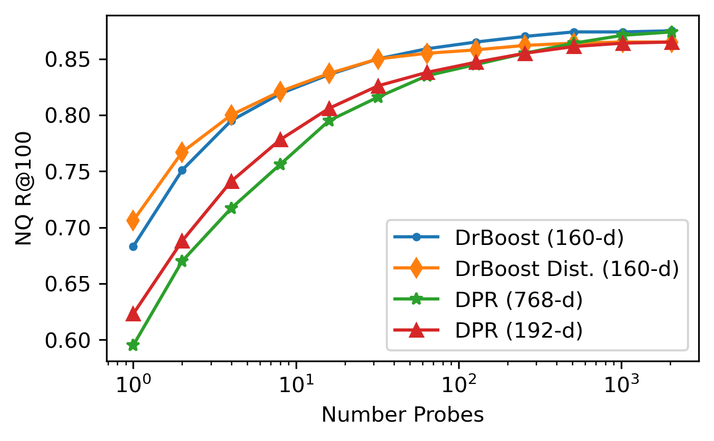
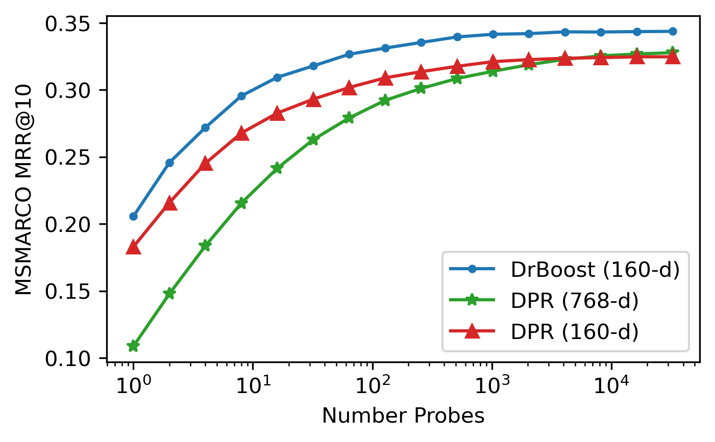
Figure 1: Search accuracy vs the number of clusters visited in IVF search (proportional to latency). Accuracy drops as search speed increases, but the accuracy drop-off for DrBoost is much slower than for DPR.

Methods	Total Dim.	Size (GB)	NQ
			R@20	R@100
DPR Yamada et al. (2021)	768	64.6	78.4	85.4
+ PQ (8-dim subvecs)		2.0	72.2	81.2
BPR Yamada et al. (2021)	768∗	2.0	77.9	85.7
DrBoost	160	13.5	80.9	87.6
+ PQ (4-dim subvecs)		0.84	80.3	86.8
+ PQ (8-dim subvecs)		0.42	76.7	84.8

Table 3: Product Quantization Results. * Indicates Binary vector.

Table 1 shows how DPR and DrBoost behave under IVF MIPS search, which is also shown graphically in figure 1. We find that DrBoost dramatically outperforms DPR in IVF search, indicating that much faster search is possible with DrBoost. High-dimensional embeddings suffer under IVF due the the curse of dimensionality, thus compact embeddings are important. Using 8 search probes, DrBoost outperforms DPR by 10.5% on MSMARCO and 6.3% on NQ R@100. The dimensionally-matched DPR is stronger, but still trails DrBoost by about 4% using 8 probes. The strongest exact search model is thus not necessarily the best in practical approximate MIPS settings. For example, if we can tolerate a 10% relative drop in accuracy from the best performing system’s exact search, DrBoost requires 16 (4) probes for MSMARCO (NQ) to reach the required accuracy, whereas DPR will require 1024 (16), meaning DrBoost can be operated approximately 64$\times$ (4$\times$) faster.

The Distilled DrBoost is also shown for NQ in Table 1. The precision (low R@K values) is essentially unaffected, (exact search drops by 0.1% for R@20), but recall drops slightly (-0.7% R@100). Interestingly, the distilled DrBoost performs even better under IVF search, improving over DrBoost by $\sim$1% at low numbers of probes. Crucially, whilst the distilled DrBoost is only slightly better than the 192-dim DPR under exact search, it is 4-5% stronger under IVF with 8 probes (alternatively, 8$\times$ faster for equivalent accuracy).

Fast retrieval is important, but we may also require small indices for edge devices, or for scalability reasons. We have already established that DrBoost can produce high quality compact embeddings, but Product Quantization can reduce this even further. Table 3 shows that DrBoost’s NQ index can be compressed from 13.5 GB to 840MB with less than 1% drop in performance. We compare to BPR Yamada et al. (2021), a method specifically designed to learn small indices by learning binary vectors. DrBoost’s PQ index is 2.4$\times$ smaller than the BPR index reported by Yamada et al. (2021), whilst being 2.4% more accurate (R@20). A more aggressive quantization leads to a 420MB index – 4.8$\times$ smaller than BPR – whilst only being 1.2% less accurate.

5 Analysis

We conduct qualitative and quantitative analysis to better understand DrBoost’s behavior.

5.1 Qualitative Analysis

Since each round’s model is learned on the errors of the previous round, we expect each learner to “specialize” and learn complementary representations. To see if this is qualitatively true, we look at the retrieved passages from each round’s retriever in isolation. Indeed, we find that each 32-dim sub-vector tackles the query from different angles. For instance, for the query “who got the first nobel prize in physics?”, the first sub-vector captures general topical similarity based on keywords, retrieving passages related to the “Nobel Prize”. The second focuses mostly on the first paragraphs of the Wikipedia articles of prominent historical personalities, presumably because these are highly likely to contain answers in general; and the third one retrieves from the pages of famous scientists and inventors. The combined DrBoost model would favor passages in the intersection of these sets. Examples can be seen in Table 10 in the Appendix.

5.2 In-distribution generalization

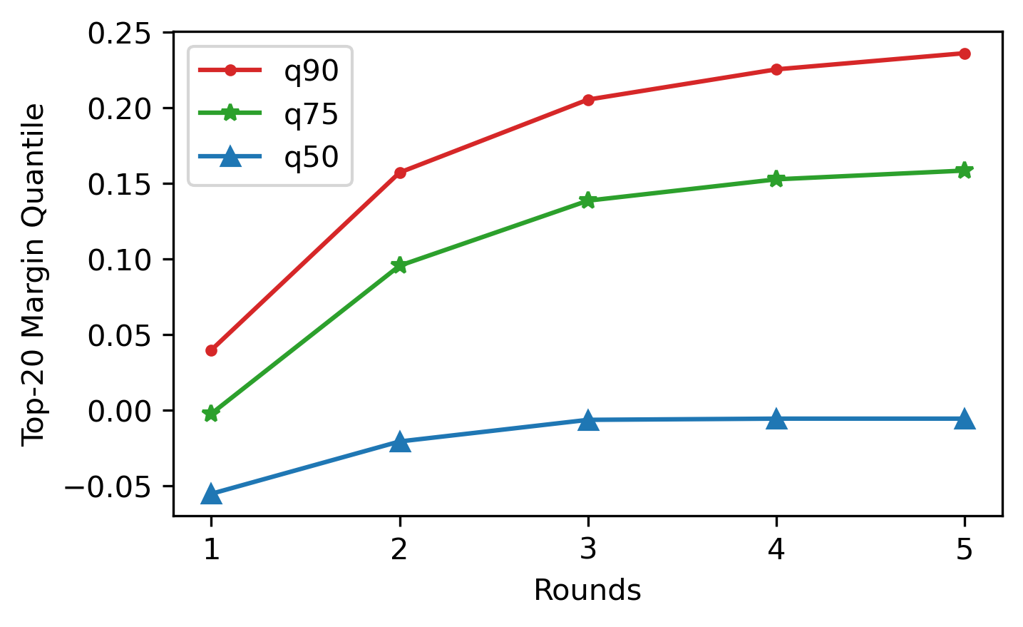
Figure 2: Quantiles of the top-20 margin on the NQ training set, for each iteration of DrBoost.

Boosting algorithms are remarkably resistant to over-fitting, even when the combined classifier has sufficient capacity to achieve zero training error. In their landmark paper, Bartlett et al. (1998) show that this desirable generalization property is a result of the following: the training margins increase with each iteration of boosting. We empirically show the same to be true for DrBoost. For a given query embedding, dense retrieval acts as a linear classifier, where the gold passage is positive and all other passages are negatives (Eq. 1). We adopt the classical definition of margin for linear classifiers to dense retrieval by defining a top-$k$ margin as follows:

$$\text{Top-k margin}_{i}=\frac{h(q_{i},c^{+})-\max_{c^{-}}^{\{k\}}h(q_{i},c^{-})}{||q_{i}||\mu_{c}}$$ (2)

where $\mu_{c}$ is the average norm of passage embeddings and the operator $\max^{\{k\}}$ returns the $k$th maximum element in the set. For a fixed $q_{i}$ and $k=1$, this definition is identical to the classical margin definition. Figure 2 plots the 50th, 75th and 90th percentiles of the top-20 margin for DrBoost on the NQ training set. We clearly see that margins indeed increase at each step, especially for cases that the model is confident in (high margin). We hypothesize this property to be the main reason for the strong in-distribution generalization of DrBoost that we observed, and potentially also for the surprisingly strong IVF results, since wide margins should intuitively make clustering easier as well.

5.3 Cross-domain generalization

Method	SciFact	FiQA	Quora	ArguAna
	NDCG@10	NDCG@10	NDCG@10	NDCG@10
SotA Dense	64.3	30.8	85.2	42.9
DPR (160 dim)	50.9	22.8	84.3	42.5
DrBoost (160 dim)	49.7	22.4	78.8	39.9

Table 4: BEIR results. The SotA row is copied from Thakur et al. (2021), and the numbers represent the best model for each dataset.

Method	EntityQuestions
	R@20	R@100
BM25 Chen et al. (2021)	71.2	79.7
DPR Chen et al. (2021)	49.7	63.4
DPR (192 dim)	47.1	60.6
DrBoost (160 dim)	51.2	63.4

Table 5: Entity Questions Results.

It has been observed in previous work Thakur et al. (2021) that dense retrievers still largely lag behind sparse retrievers in terms of generalization capabilities. We are interested to test whether our method could be beneficial for out-of-domain transfer as well. We show the results for zero-shot transfer on a subset of the BEIR benchmark in Table 4 and the EntityQuestions dataset in Table 5. While DrBoost improves slightly over the dimension-matched baseline on EntityQuestions, where the passage corpora stays the same, it produces worse results on the BEIR datasets. We conclude that boosting is not especially useful for cross-domain transfer, and should be combined with other methods if this is a concern. We leave this for future work.

5.4 Representation Probing

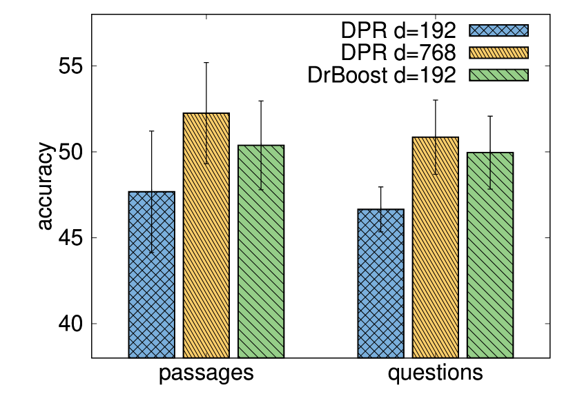
Figure 3: Topic classification accuracy when probing DrBoost and DPR representations with an SVM.

One of the hypothesis we formulate for the stronger performance of DrBoost over DPR is that the former might better capture topical information of passages and questions. To test this, we collected topics for all Wikipedia articles in Natural Questions using the strategy of Johnson et al. (2021) and associate them with both passages and questions. We then probed both DPR and DrBoost representations with an SVM Steinwart and Christmann (2008) classifier considering a 5-fold cross-validation over 500 instances and 8 different seeds. Results (in Figure 3) confirms our hypothesis: the topic classifier accuracy is higher with DrBoost representations with respect to DPR ones of the same dimension (i.e., 192), for both questions and passages.

6 Related Work

Boosting for retrieval

Boosting has been studied in machine learning for over three decades Kearns and Valiant (1989); Schapire (1990). Models such as AdaBoost Freund and Schapire (1997) and GBMs Friedman (2001) became popular approaches to classification problems, with implementations such as XGBoost still popular today Chen and Guestrin (2016). Many boosting approaches have been proposed for retrieval and learning-to-rank (LTR) problems, typically employing decision trees, such as AdaRank Xu and Li (2007), RankBoost Freund et al. (2003) and lamdaMART Wu et al. (2009). Apart from speed and accuracy, boosting is attractive due to promising theoretical properties such as convergence and generalization. Bartlett et al. (1998); Freund et al. (2003); Mohri et al. (2012). Boosted decision trees have recently been demonstrated to be competitive on LTR tasks Qin et al. (2021), but, in recent years, boosting approaches have generally received less attention, as (pretrained) neural models began to dominate much of the literature. However, modern neural models and boosting techniques need not be exclusive, and a small amount of work exploring boosting in the context of modern pre-trained neural models has been carried out Huang et al. (2020); Qin et al. (2021). Our work follows this line of thinking, identifying dimensionally-constrained bi-encoders as good candidates as neural weak learners, adopting a simple boosting approach which allows for simple and efficient MIPS at test time.

Dense Retrieval

Sparse, term-based Retrievers such as BM25 Robertson and Zaragoza (2009) have dominated retrieval until recently. Dense, MIPS-based Retrieval using bi-encoder architectures leveraging contrastive training with gold pairs Yih et al. (2011) has recently shown to be effective in several settings Lee et al. (2019); Karpukhin et al. (2020); Reimers and Gurevych (2019); Hofstätter et al. (2021b). See Yates et al. (2021) for a survey. The success of Dense Retrieval has led to many recent papers proposing schemes to improve dense retriever training by innovating on how negatives are sampled (Xiong et al., 2020; Qu et al., 2021; Zhan et al., 2021c; Lin et al., 2021, inter alia.), and/or proposing pretraining objectives Oğuz et al. (2021); Guu et al. (2020); Chang et al. (2020); Sachan et al. (2021); Gao and Callan (2021). Our work also innovates on how dense retrievers are trained, but is arguably orthogonal to most of these training innovations, since these could still be employed when training each component weak learner.

Distillation

We leverage a simple distillation technique to make DrBoost more efficient at test time. Distillation for dense retrievers is an active area, and more complex schemes exist which could improve results further Izacard and Grave (2021); Qu et al. (2021); Yang and Seo (2020); Lin et al. (2021); Hofstätter et al. (2021a); Barkan et al. (2020); Gao et al. (2020).

Multi-vector Retrievers

Several approaches represent passages with multiple vectors. Humeau et al. (2020) represent queries with multiple vectors, but retrieval is comparatively slow as relevance cannot be calculated with a single MIPS call. ME-BERT Luan et al. (2021) index a fixed number of vectors for each passage and ColBERT Khattab and Zaharia (2020) index a vector for every word. Both can perform retrieval with a single MIPS call (although ColBERT requires reranking) but produce very large indices, which, in turn, slows down search. DrBoost can also be seen as a multi-vector approach, with each weak learner producing a vector. However, each vector is small, and we index concatenated vectors, rather than indexing each vector independently, leading to small indices and fast search. This said, adapting DrBoost-style training to these settings would be feasible. SPAR Chen et al. (2021) is a two-vector method: one from a standard dense retriever, and the other from a more lexically-oriented model. SPAR uses a similar test-time MIPS retrieval strategy to ours, and SPAR’s lexical embeddings could be trivially added to DrBoost as an additional subvector.

Efficient retrievers

There have been a number of recent efforts to build more efficient retrieval and question answering systems Min et al. (2021). Izacard et al. (2020) and Yang and Seo (2021) experiment with post-hoc compression and lower-dimensional embeddings, Lewis et al. (2021) index and retrieve question-answer pairs and Yamada et al. (2021) propose BPR, which approximates MIPS using binary vectors. There is also a line of work learning embeddings specifically suited for approximate search Yu et al. (2018); Zhan et al. (2021a, b) Generative retrievers De Cao et al. (2021) can also be very efficient. DrBoost also employs lower-dimensional embeddings and off-the-shelf post-hoc compression for its smallest index, producing smaller indices than BPR, whilst also being more accurate.

7 Discussion

In this work we have explored boosting in the context of dense retrieval, inspired by the similarity of iteratively-sampling negatives to boosting. We find that our simple boosting approach, DrBoost, performs largely on par with a 768-dimensional DPR baseline, but produces more compact vectors, and is more amenable to approximate search. We note that DrBoost requires maintaining more neural models at test time, which may put a greater demand on GPU resources. However the models can be run in parallel if latency is a concern, and if needed, these models can be distilled into a single model with little drop in accuracy. We hope that future work will build on boosting approaches for dense retrieval, including adding adaptive weights, and investigating alternative losses and sampling techniques. We also suggest that emphasis in dense retrieval should be placed on more holistic evaluation than just exact retrieval accuracy, demonstrating that models with quite similar exact retrieval can perform very differently under practically-important approximate search settings.

Appendix A Appendix

	DrBoost			DPR			DPR, 160 dim.
	(n=4096)	(n=16384)	(n=65536)	(n=4096)	(n=16384)	(n=65536)	(n=4096)	(n=16384)	(n=65536)
Exhaustive	0.3438	0.3438	0.3438	0.328	0.328	0.328	0.3248	0.3248	0.3248
1	0.1905	0.1884	0.2057	0.1277	0.1186	0.1088	0.1669	0.1637	0.183
2	0.2338	0.2359	0.2458	0.172	0.1599	0.1479	0.2129	0.2072	0.2159
4	0.2694	0.2652	0.2719	0.2095	0.1996	0.1836	0.2465	0.2395	0.2452
8	0.2919	0.2873	0.2955	0.2433	0.2326	0.2155	0.2722	0.2637	0.2678
16	0.3106	0.3018	0.3094	0.2693	0.2532	0.2415	0.2906	0.2822	0.2827
32	0.324	0.3161	0.3179	0.2855	0.2715	0.2629	0.3027	0.297	0.2931
64	0.3314	0.3236	0.3266	0.2994	0.2864	0.2791	0.3127	0.3063	0.3018
128	0.3382	0.332	0.3312	0.31	0.2982	0.2922	0.3179	0.3129	0.309
256	0.34	0.3375	0.3354	0.3161	0.3092	0.3011	0.3206	0.3182	0.3136
512	0.3424	0.34	0.3395	0.3226	0.3141	0.3085	0.3232	0.3212	0.3176
1024	0.3437	0.3416	0.3415	0.325	0.3197	0.3139	0.3243	0.3229	0.3211
2048	0.3438	0.343	0.342	0.3279	0.3243	0.3188	0.3247	0.3242	0.3226
4096		0.3435	0.3433		0.3268	0.3228		0.3249	0.3236
8192		0.3438	0.3432		0.3278	0.3254		0.3248	0.3241
16384			0.3435			0.3268			0.3247
32768			0.3437			0.3278			0.3247

Table 6: IVF indexing results on MSMARCO. Metric is MRR@10. $n$ refers to number of clusters used for IVF training.

	DrBoost, 160 dim	DrBoost-distilled, 160 dim	DrBoost, 192 dim	DrBoost-distilled, 192 dim	DPR	DPR, 192 dim.
Exhaustive	0.876	0.868	0.874	0.870	0.879	0.866
1	0.683	0.706	0.684	0.701	0.595	0.623
2	0.751	0.767	0.750	0.760	0.670	0.688
4	0.795	0.800	0.793	0.803	0.717	0.741
8	0.819	0.821	0.819	0.825	0.756	0.778
16	0.836	0.837	0.835	0.840	0.795	0.806
32	0.850	0.849	0.845	0.848	0.816	0.826
64	0.859	0.855	0.858	0.856	0.835	0.838
128	0.865	0.858	0.864	0.859	0.845	0.847
256	0.870	0.862	0.868	0.863	0.855	0.855
512	0.874	0.864	0.870	0.866	0.864	0.861
1024	0.874	0.865	0.871	0.866	0.871	0.864
2048	0.875	0.865	0.873	0.867	0.874	0.865

Table 7: IVF indexing results on NQ. Metric is Recall@100. The number of clusters used for IVF training was 65536.

	DrBoost, 160 dim	DrBoost-distilled, 160 dim	DrBoost, 192 dim	DrBoost-distilled, 192 dim	DPR	DPR, 192 dim.
Exhaustive	0.809	0.809	0.813	0.809	0.827	0.808
1	0.624	0.650	0.625	0.647	0.518	0.557
2	0.686	0.703	0.684	0.703	0.597	0.625
4	0.732	0.744	0.730	0.746	0.647	0.679
8	0.758	0.764	0.755	0.764	0.690	0.717
16	0.771	0.779	0.775	0.780	0.732	0.743
32	0.784	0.793	0.786	0.791	0.760	0.766
64	0.794	0.797	0.799	0.799	0.779	0.780
128	0.799	0.800	0.805	0.801	0.791	0.789
256	0.804	0.803	0.810	0.804	0.803	0.797
512	0.807	0.805	0.812	0.807	0.813	0.803
1024	0.808	0.806	0.812	0.807	0.820	0.805
2048	0.808	0.806	0.813	0.808	0.823	0.807

Table 8: IVF indexing results on NQ. Metric is Recall@20. The number of clusters used for IVF training was 65536.

	DrBoost, 160 dim	DrBoost-distilled, 160 dim	DrBoost, 192 dim	DrBoost-distilled, 192 dim	DPR	DPR, 192 dim.
Exhaustive	0.710	0.706	0.715	0.703	0.731	0.710
1	0.544	0.560	0.535	0.557	0.439	0.475
2	0.597	0.615	0.594	0.605	0.506	0.540
4	0.634	0.646	0.636	0.644	0.551	0.593
8	0.662	0.663	0.663	0.665	0.597	0.623
16	0.678	0.676	0.681	0.680	0.640	0.653
32	0.691	0.689	0.692	0.688	0.666	0.671
64	0.699	0.692	0.702	0.695	0.687	0.685
128	0.704	0.696	0.708	0.699	0.698	0.694
256	0.707	0.701	0.710	0.702	0.709	0.703
512	0.709	0.703	0.712	0.703	0.718	0.707
1024	0.710	0.704	0.713	0.703	0.726	0.708
2048	0.710	0.704	0.714	0.704	0.728	0.709

Table 9: IVF indexing results on NQ. Metric is Recall@5. The number of clusters used for IVF training was 65536.

Rounds	who got the first nobel prize in physics?	when is the next deadpool movie being released?
1	0: Title: Nobel Prize in Physics The Nobel Prize in Physics is a yearly award given by the Royal Swedish Academy of Sciences for those who have made the … 1: Title: Nobel Prize in Physics …receive a diploma, a medal and a document confirming the prize amount. Nobel Prize in Physics … 2: Title: Nobel Prize controversies …research CERN, commented in a scientific meet in Kolkata titled ”Frontiers of Science” that ”it is unfortunate that pioneering …	0: Title: Deadpool (film) …was written by Reese and Wernick and played in front of ”Logan”. ”Deadpool 2” was released on May 18, 2018, with … 1: Title: Deadpool 2 …chimichangas, traditionally Deadpool’s favorite food, as well as ”Deadpool”-inspired Harder drinks. The campaign also … 2: Title: Deadpool 2 …the final two hours. By May 2018, Leitch was working on an official extended edition of the film with Fox wanting to ”spin that …
2	0: Title: George B. McClellan George Brinton McClellan (December 3, 1826-October 29, 1885) was an American soldier, civil engineer, railroad executive … 1: Title: Johannes Brahms Johannes Brahms (; 7 May 1833 – 3 April 1897) was a German composer and pianist of the Romantic period. Born in Hamburg … 2: Title: Bede Bede ( ; ; 672/3 – 26 May 735), also known as Saint Bede, Venerable Bede, and Bede the Venerable (), was an English Benedictine …	0: Title: Here and Now (2018 TV series) Here and Now is an American drama television series created by Alan Ball. The series consists of ten episodes and … 1: Title: Deadpool 2 …is dedicated to her memory. The film’s score is the first to receive a parental advisory warning for explicit content, and … 2: Title: I’m New Here I’m New Here is the 13th and final studio album by American vocalist and pianist Gil Scott-Heron. It was released on February …
3	0: Title: Henri Poincare Jules Henri Poincaré (; ; 29 April 1854 – 17 July 1912) was a French mathematician, theoretical physicist, engineer, and … 1: Title: Marie Curie …named in her honor. Marie Curie Marie Skłodowska Curie (; ; ; born Maria Salomea Skłodowska; 7 November 18674 July 1934 … 2: Title: Alberto Santos-Dumont Alberto Santos-Dumont (; 20 July 187323 July 1932, usually referred to as simply Santos-Dumont) was a Brazilian inventor …	0: Title: Deadpool 2 …is dedicated to her memory. The film’s score is the first to receive a parental advisory warning for explicit content, and … 1: Title: Deadpool (film) …was written by Reese and Wernick and played in front of ”Logan”. ”Deadpool 2” was released on May 18, 2018, with … 2: Title: Kong: Skull Island …later moved to Warner Bros. in order to develop a shared cinematic universe featuring Godzilla and King Kong. …

Table 10: Example retrieval results from each round of DrBoost. Only the beginning of each passage is shown.

References

- Bajaj et al. (2016) Payal Bajaj, Daniel Campos, Nick Craswell, Li Deng, Jianfeng Gao, Xiaodong Liu, Rangan Majumder, Andrew McNamara, Bhaskar Mitra, Tri Nguyen, Mir Rosenberg, Xia Song, Alina Stoica, Saurabh Tiwary, and Tong Wang. 2016. MS MARCO: A Human Generated MAchine Reading COmprehension Dataset. arXiv:1611.09268 [cs]. ArXiv: 1611.09268.
- Barkan et al. (2020) Oren Barkan, Noam Razin, Itzik Malkiel, Ori Katz, Avi Caciularu, and Noam Koenigstein. 2020. Scalable Attentive Sentence Pair Modeling via Distilled Sentence Embedding. Proceedings of the AAAI Conference on Artificial Intelligence, 34(04):3235–3242. Number: 04.
- Bartlett et al. (1998) Peter Bartlett, Yoav Freund, Wee Sun Lee, and Robert E. Schapire. 1998. Boosting the margin: a new explanation for the effectiveness of voting methods. The Annals of Statistics, 26(5):1651 – 1686. Publisher: Institute of Mathematical Statistics.
- Chang et al. (2020) Wei-Cheng Chang, Felix X. Yu, Yin-Wen Chang, Yiming Yang, and Sanjiv Kumar. 2020. Pre-training Tasks for Embedding-based Large-scale Retrieval. arXiv:2002.03932 [cs, stat]. ArXiv: 2002.03932.
- Chen et al. (2017) Danqi Chen, Adam Fisch, Jason Weston, and Antoine Bordes. 2017. Reading Wikipedia to Answer Open-Domain Questions. In Proceedings of the 55th Annual Meeting of the Association for Computational Linguistics (Volume 1: Long Papers), pages 1870–1879, Vancouver, Canada. Association for Computational Linguistics.
- Chen and Guestrin (2016) Tianqi Chen and Carlos Guestrin. 2016. XGBoost: A Scalable Tree Boosting System. In Proceedings of the 22nd ACM SIGKDD International Conference on Knowledge Discovery and Data Mining, KDD ’16, pages 785–794, New York, NY, USA. ACM. Event-place: San Francisco, California, USA.
- Chen et al. (2021) Xilun Chen, Kushal Lakhotia, Barlas Oğuz, Anchit Gupta, Patrick Lewis, Stan Peshterliev, Yashar Mehdad, Sonal Gupta, and Wen-tau Yih. 2021. Salient Phrase Aware Dense Retrieval: Can a Dense Retriever Imitate a Sparse One? arXiv:2110.06918 [cs]. ArXiv: 2110.06918.
- De Cao et al. (2021) Nicola De Cao, Gautier Izacard, Sebastian Riedel, and Fabio Petroni. 2021. Autoregressive Entity Retrieval. In International Conference on Learning Representations.
- Freund et al. (2003) Yoav Freund, Raj Iyer, Robert E. Schapire, and Yoram Singer. 2003. An Efficient Boosting Algorithm for Combining Preferences. J. Mach. Learn. Res., 4(null):933–969. Publisher: JMLR.org.
- Freund and Schapire (1997) Yoav Freund and Robert E. Schapire. 1997. A Decision-Theoretic Generalization of On-Line Learning and an Application to Boosting. Journal of Computer and System Sciences, 55(1):119–139.
- Friedman (2001) Jerome H. Friedman. 2001. Greedy function approximation: A gradient boosting machine. Annals of Statistics, 29(5):1189–1232. Publisher: Institute of Mathematical Statistics.
- Gao and Callan (2021) Luyu Gao and Jamie Callan. 2021. Condenser: a Pre-training Architecture for Dense Retrieval. In Proceedings of the 2021 Conference on Empirical Methods in Natural Language Processing, pages 981–993, Online and Punta Cana, Dominican Republic. Association for Computational Linguistics.
- Gao et al. (2020) Luyu Gao, Zhuyun Dai, and Jamie Callan. 2020. Understanding BERT Rankers Under Distillation. In Proceedings of the 2020 ACM SIGIR on International Conference on Theory of Information Retrieval, ICTIR ’20, pages 149–152, New York, NY, USA. Association for Computing Machinery.
- Guu et al. (2020) Kelvin Guu, Kenton Lee, Zora Tung, Panupong Pasupat, and Ming-Wei Chang. 2020. Retrieval Augmented Language Model Pre-Training. In Proceedings of the 37th International Conference on Machine Learning, ICML 2020, 13-18 July 2020, Virtual Event, volume 119 of Proceedings of Machine Learning Research, pages 3929–3938. PMLR.
- Hofstätter et al. (2021a) Sebastian Hofstätter, Sophia Althammer, Michael Schröder, Mete Sertkan, and Allan Hanbury. 2021a. Improving Efficient Neural Ranking Models with Cross-Architecture Knowledge Distillation. arXiv:2010.02666 [cs]. ArXiv: 2010.02666.
- Hofstätter et al. (2021b) Sebastian Hofstätter, Sheng-Chieh Lin, Jheng-Hong Yang, Jimmy Lin, and Allan Hanbury. 2021b. Efficiently Teaching an Effective Dense Retriever with Balanced Topic Aware Sampling. In Proceedings of the 44th International ACM SIGIR Conference on Research and Development in Information Retrieval, SIGIR ’21, pages 113–122, New York, NY, USA. Association for Computing Machinery. Event-place: Virtual Event, Canada.
- Huang et al. (2020) Tongwen Huang, Qingyun She, and Junlin Zhang. 2020. BoostingBERT:Integrating Multi-Class Boosting into BERT for NLP Tasks. arXiv:2009.05959 [cs]. ArXiv: 2009.05959.
- Humeau et al. (2020) Samuel Humeau, Kurt Shuster, Marie-Anne Lachaux, and Jason Weston. 2020. Poly-encoders: Architectures and Pre-training Strategies for Fast and Accurate Multi-sentence Scoring. In International Conference on Learning Representations.
- Izacard and Grave (2021) Gautier Izacard and Edouard Grave. 2021. Distilling Knowledge from Reader to Retriever for Question Answering. In International Conference on Learning Representations.
- Izacard et al. (2020) Gautier Izacard, Fabio Petroni, Lucas Hosseini, Nicola De Cao, Sebastian Riedel, and Edouard Grave. 2020. A Memory Efficient Baseline for Open Domain Question Answering. arXiv:2012.15156 [cs]. ArXiv: 2012.15156.
- Johnson et al. (2021) Isaac Johnson, Martin Gerlach, and Diego Sáez-Trumper. 2021. Language-agnostic topic classification for wikipedia. In Companion Proceedings of the Web Conference 2021, pages 594–601.
- Johnson et al. (2019) Jeff Johnson, Matthijs Douze, and Hervé Jégou. 2019. Billion-scale similarity search with GPUs. IEEE Transactions on Big Data, pages 1–1.
- Jégou et al. (2011) H Jégou, M Douze, and C Schmid. 2011. Product Quantization for Nearest Neighbor Search. IEEE Transactions on Pattern Analysis and Machine Intelligence, 33(1):117–128.
- Karpukhin et al. (2020) Vladimir Karpukhin, Barlas Oguz, Sewon Min, Patrick Lewis, Ledell Wu, Sergey Edunov, Danqi Chen, and Wen-tau Yih. 2020. Dense Passage Retrieval for Open-Domain Question Answering. In Proceedings of the 2020 Conference on Empirical Methods in Natural Language Processing (EMNLP), pages 6769–6781, Online. Association for Computational Linguistics.
- Kearns and Valiant (1989) M. Kearns and L. G. Valiant. 1989. Crytographic Limitations on Learning Boolean Formulae and Finite Automata. In Proceedings of the Twenty-First Annual ACM Symposium on Theory of Computing, STOC ’89, pages 433–444, New York, NY, USA. Association for Computing Machinery. Event-place: Seattle, Washington, USA.
- Khattab and Zaharia (2020) Omar Khattab and Matei Zaharia. 2020. ColBERT: Efficient and Effective Passage Search via Contextualized Late Interaction over BERT. In Proceedings of the 43rd International ACM SIGIR Conference on Research and Development in Information Retrieval, pages 39–48, Virtual Event China. ACM.
- Kwiatkowski et al. (2019) Tom Kwiatkowski, Jennimaria Palomaki, Olivia Redfield, Michael Collins, Ankur Parikh, Chris Alberti, Danielle Epstein, Illia Polosukhin, Matthew Kelcey, Jacob Devlin, Kenton Lee, Kristina N. Toutanova, Llion Jones, Ming-Wei Chang, Andrew Dai, Jakob Uszkoreit, Quoc Le, and Slav Petrov. 2019. Natural Questions: a Benchmark for Question Answering Research. Transactions of the Association of Computational Linguistics, 7:452–466.
- Lee et al. (2019) Kenton Lee, Ming-Wei Chang, and Kristina Toutanova. 2019. Latent Retrieval for Weakly Supervised Open Domain Question Answering. In Proceedings of the 57th Annual Meeting of the Association for Computational Linguistics, pages 6086–6096, Florence, Italy. Association for Computational Linguistics.
- Lewis et al. (2020) Patrick Lewis, Ethan Perez, Aleksandra Piktus, Fabio Petroni, Vladimir Karpukhin, Naman Goyal, Heinrich Küttler, Mike Lewis, Wen-tau Yih, Tim Rocktäschel, Sebastian Riedel, and Douwe Kiela. 2020. Retrieval-Augmented Generation for Knowledge-Intensive NLP Tasks. In Advances in Neural Information Processing Systems, volume 33, pages 9459–9474. Curran Associates, Inc.
- Lewis et al. (2021) Patrick Lewis, Yuxiang Wu, Linqing Liu, Pasquale Minervini, Heinrich Küttler, Aleksandra Piktus, Pontus Stenetorp, and Sebastian Riedel. 2021. PAQ: 65 Million Probably-Asked Questions and What You Can Do With Them. Transactions of the Association for Computational Linguistics, 9(0):1098–1115.
- Lin et al. (2021) Sheng-Chieh Lin, Jheng-Hong Yang, and Jimmy Lin. 2021. In-Batch Negatives for Knowledge Distillation with Tightly-Coupled Teachers for Dense Retrieval. In Proceedings of the 6th Workshop on Representation Learning for NLP (RepL4NLP-2021), pages 163–173, Online. Association for Computational Linguistics.
- Lloyd (1982) S. Lloyd. 1982. Least squares quantization in PCM. IEEE Transactions on Information Theory, 28(2):129–137.
- Luan et al. (2021) Yi Luan, Jacob Eisenstein, Kristina Toutanova, and Michael Collins. 2021. Sparse, Dense, and Attentional Representations for Text Retrieval. Transactions of the Association for Computational Linguistics, 9:329–345.
- Malkov and Yashunin (2020) Yu A. Malkov and D. A. Yashunin. 2020. Efficient and Robust Approximate Nearest Neighbor Search Using Hierarchical Navigable Small World Graphs. IEEE Transactions on Pattern Analysis and Machine Intelligence, 42(4):824–836.
- Matsui et al. (2018) Yusuke Matsui, Yusuke Uchida, Herve Jegou, and Shin’ichi Satoh. 2018. Paper A Survey of Product Quantization. 6(1):9.
- Min et al. (2021) Sewon Min, Jordan Boyd-Graber, Chris Alberti, Danqi Chen, Eunsol Choi, Michael Collins, Kelvin Guu, Hannaneh Hajishirzi, Kenton Lee, Jennimaria Palomaki, Colin Raffel, Adam Roberts, Tom Kwiatkowski, Patrick Lewis, Yuxiang Wu, Heinrich Küttler, Linqing Liu, Pasquale Minervini, Pontus Stenetorp, Sebastian Riedel, Sohee Yang, Minjoon Seo, Gautier Izacard, Fabio Petroni, Lucas Hosseini, Nicola De Cao, Edouard Grave, Ikuya Yamada, Sonse Shimaoka, Masatoshi Suzuki, Shumpei Miyawaki, Shun Sato, Ryo Takahashi, Jun Suzuki, Martin Fajcik, Martin Docekal, Karel Ondrej, Pavel Smrz, Hao Cheng, Yelong Shen, Xiaodong Liu, Pengcheng He, Weizhu Chen, Jianfeng Gao, Barlas Oguz, Xilun Chen, Vladimir Karpukhin, Stan Peshterliev, Dmytro Okhonko, Michael Schlichtkrull, Sonal Gupta, Yashar Mehdad, and Wen-tau Yih. 2021. NeurIPS 2020 EfficientQA Competition: Systems, Analyses and Lessons Learned. In Proceedings of the NeurIPS 2020 Competition and Demonstration Track, volume 133 of Proceedings of Machine Learning Research, pages 86–111. PMLR.
- Mohri et al. (2012) Mehryar Mohri, Afshin Rostamizadeh, and Ameet Talwalkar. 2012. Foundations of machine learning. Cambridge, MA: MIT Press. Journal Abbreviation: Adapt. Comput. Mach. Learn. Publication Title: Adaptive Computation and Machine Learning.
- Oğuz et al. (2021) Barlas Oğuz, Kushal Lakhotia, Anchit Gupta, Patrick Lewis, Vladimir Karpukhin, Aleksandra Piktus, Xilun Chen, Sebastian Riedel, Wen-tau Yih, Sonal Gupta, and Yashar Mehdad. 2021. Domain-matched Pre-training Tasks for Dense Retrieval. arXiv:2107.13602 [cs]. ArXiv: 2107.13602.
- Petroni et al. (2021) Fabio Petroni, Aleksandra Piktus, Angela Fan, Patrick Lewis, Majid Yazdani, Nicola De Cao, James Thorne, Yacine Jernite, Vladimir Karpukhin, Jean Maillard, Vassilis Plachouras, Tim Rocktäschel, and Sebastian Riedel. 2021. KILT: a Benchmark for Knowledge Intensive Language Tasks. In Proceedings of the 2021 Conference of the North American Chapter of the Association for Computational Linguistics: Human Language Technologies, pages 2523–2544, Online. Association for Computational Linguistics.
- Qin et al. (2021) Zhen Qin, Le Yan, Honglei Zhuang, Yi Tay, Rama Kumar Pasumarthi, Xuanhui Wang, Michael Bendersky, and Marc Najork. 2021. Are Neural Rankers still Outperformed by Gradient Boosted Decision Trees? In International Conference on Learning Representations.
- Qu et al. (2021) Yingqi Qu, Yuchen Ding, Jing Liu, Kai Liu, Ruiyang Ren, Wayne Xin Zhao, Daxiang Dong, Hua Wu, and Haifeng Wang. 2021. RocketQA: An Optimized Training Approach to Dense Passage Retrieval for Open-Domain Question Answering. arXiv:2010.08191 [cs]. ArXiv: 2010.08191.
- Reimers and Gurevych (2019) Nils Reimers and Iryna Gurevych. 2019. Sentence-BERT: Sentence Embeddings using Siamese BERT-Networks. In Proceedings of the 2019 Conference on Empirical Methods in Natural Language Processing and the 9th International Joint Conference on Natural Language Processing (EMNLP-IJCNLP), pages 3982–3992, Hong Kong, China. Association for Computational Linguistics.
- Robertson (2008) Stephen Robertson. 2008. On the history of evaluation in IR. Journal of Information Science, 34(4):439–456. _eprint: https://doi.org/10.1177/0165551507086989.
- Robertson and Zaragoza (2009) Stephen Robertson and Hugo Zaragoza. 2009. The Probabilistic Relevance Framework: BM25 and Beyond. Found. Trends Inf. Retr., 3(4):333–389. Place: Hanover, MA, USA Publisher: Now Publishers Inc.
- Sachan et al. (2021) Devendra Sachan, Mostofa Patwary, Mohammad Shoeybi, Neel Kant, Wei Ping, William L. Hamilton, and Bryan Catanzaro. 2021. End-to-End Training of Neural Retrievers for Open-Domain Question Answering. In Proceedings of the 59th Annual Meeting of the Association for Computational Linguistics and the 11th International Joint Conference on Natural Language Processing (Volume 1: Long Papers), pages 6648–6662, Online. Association for Computational Linguistics.
- Schapire (2007) Rob Schapire. 2007. Theory and Applications of Boosting. In Neural Information Processing Systems, Tutorials, page 104.
- Schapire (1990) Robert E. Schapire. 1990. The strength of weak learnability. Machine Learning, 5(2):197–227.
- Sciavolino et al. (2021) Christopher Sciavolino, Zexuan Zhong, Jinhyuk Lee, and Danqi Chen. 2021. Simple Entity-Centric Questions Challenge Dense Retrievers. arXiv:2109.08535 [cs]. ArXiv: 2109.08535.
- Sivic and Zisserman (2003) Sivic and Zisserman. 2003. Video Google: a text retrieval approach to object matching in videos. In Proceedings Ninth IEEE International Conference on Computer Vision, pages 1470–1477 vol.2.
- Steinwart and Christmann (2008) Ingo Steinwart and Andreas Christmann. 2008. Support vector machines. Springer Science & Business Media.
- Thakur et al. (2021) Nandan Thakur, Nils Reimers, Andreas Rücklé, Abhishek Srivastava, and Iryna Gurevych. 2021. BEIR: A Heterogenous Benchmark for Zero-shot Evaluation of Information Retrieval Models. CoRR, abs/2104.08663. ArXiv: 2104.08663.
- Thorne et al. (2018) James Thorne, Andreas Vlachos, Christos Christodoulopoulos, and Arpit Mittal. 2018. FEVER: a Large-scale Dataset for Fact Extraction and VERification. In Proceedings of the 2018 Conference of the North American Chapter of the Association for Computational Linguistics: Human Language Technologies, Volume 1 (Long Papers), pages 809–819, New Orleans, Louisiana. Association for Computational Linguistics.
- Voorhees and Tice (2000) Ellen M. Voorhees and Dawn M. Tice. 2000. Building a Question Answering Test Collection. In Proceedings of the 23rd Annual International ACM SIGIR Conference on Research and Development in Information Retrieval, SIGIR ’00, pages 200–207, New York, NY, USA. ACM. Event-place: Athens, Greece.
- Wu et al. (2009) Qiang Wu, C. Burges, K. Svore, and Jianfeng Gao. 2009. Adapting boosting for information retrieval measures. Information Retrieval.
- Xiong et al. (2020) Lee Xiong, Chenyan Xiong, Ye Li, Kwok-Fung Tang, Jialin Liu, Paul Bennett, Junaid Ahmed, and Arnold Overwijk. 2020. Approximate Nearest Neighbor Negative Contrastive Learning for Dense Text Retrieval. arXiv:2007.00808 [cs]. ArXiv: 2007.00808.
- Xu and Li (2007) Jun Xu and Hang Li. 2007. AdaRank: a boosting algorithm for information retrieval. In SIGIR.
- Yamada et al. (2021) Ikuya Yamada, Akari Asai, and Hannaneh Hajishirzi. 2021. Efficient Passage Retrieval with Hashing for Open-domain Question Answering. arXiv:2106.00882 [cs]. ArXiv: 2106.00882.
- Yang et al. (2017) Peilin Yang, Hui Fang, and Jimmy Lin. 2017. Anserini: Enabling the use of Lucene for information retrieval research. In Proceedings of the 40th International ACM SIGIR Conference on Research and Development in Information Retrieval, pages 1253–1256.
- Yang and Seo (2020) Sohee Yang and Minjoon Seo. 2020. Is Retriever Merely an Approximator of Reader? arXiv:2010.10999 [cs]. ArXiv: 2010.10999.
- Yang and Seo (2021) Sohee Yang and Minjoon Seo. 2021. Designing a Minimal Retrieve-and-Read System for Open-Domain Question Answering. arXiv:2104.07242 [cs]. ArXiv: 2104.07242.
- Yates et al. (2021) Andrew Yates, Rodrigo Nogueira, and Jimmy Lin. 2021. Pretrained Transformers for Text Ranking: BERT and Beyond. In Proceedings of the 14th ACM International Conference on Web Search and Data Mining, WSDM ’21, pages 1154–1156, New York, NY, USA. Association for Computing Machinery. Event-place: Virtual Event, Israel.
- Yih et al. (2011) Wen-tau Yih, Kristina Toutanova, John C. Platt, and Christopher Meek. 2011. Learning Discriminative Projections for Text Similarity Measures. In Proceedings of the Fifteenth Conference on Computational Natural Language Learning, CoNLL ’11, pages 247–256, USA. Association for Computational Linguistics. Event-place: Portland, Oregon.
- Yu et al. (2018) Tan Yu, Junsong Yuan, Chen Fang, and Hailin Jin. 2018. Product Quantization Network for Fast Image Retrieval. In Computer Vision – ECCV 2018, volume 11205, pages 191–206, Cham. Springer International Publishing. Series Title: Lecture Notes in Computer Science.
- Zhan et al. (2021a) Jingtao Zhan, Jiaxin Mao, Yiqun Liu, Jiafeng Guo, Min Zhang, and Shaoping Ma. 2021a. Jointly Optimizing Query Encoder and Product Quantization to Improve Retrieval Performance. arXiv:2108.00644 [cs]. ArXiv: 2108.00644.
- Zhan et al. (2021b) Jingtao Zhan, Jiaxin Mao, Yiqun Liu, Jiafeng Guo, Min Zhang, and Shaoping Ma. 2021b. Learning Discrete Representations via Constrained Clustering for Effective and Efficient Dense Retrieval. arXiv:2110.05789 [cs]. ArXiv: 2110.05789 version: 1.
- Zhan et al. (2021c) Jingtao Zhan, Jiaxin Mao, Yiqun Liu, Jiafeng Guo, Min Zhang, and Shaoping Ma. 2021c. Optimizing Dense Retrieval Model Training with Hard Negatives. arXiv:2104.08051 [cs]. ArXiv: 2104.08051.
- Zhang et al. (2021) Hang Zhang, Yeyun Gong, Yelong Shen, Jiancheng Lv, Nan Duan, and Weizhu Chen. 2021. Adversarial retriever-ranker for dense text retrieval. arXiv preprint arXiv:2110.03611.