Separate Exchangeability as Modeling Principle in Bayesian Nonparametrics

Abstract

We argue for the use of separate exchangeability as a modeling principle in Bayesian inference, especially for nonparametric Bayesian models. While in some areas, such as random graphs, separate and (closely related) joint exchangeability are widely used, and it naturally arises for example in simple mixed models, it is curiously underused for other applications. We briefly review the definition of separate exchangeability. We then discuss two specific models that implement separate exchangeability. One example is about nested random partitions for a data matrix, defining a partition of columns and nested partitions of rows, nested within column clusters. Many recently proposed models for nested partitions implement partially exchangeable models. We argue that inference under such models in some cases ignores important features of the experimental setup. The second example is about setting up separately exchangeable priors for a nonparametric regression model when multiple sets of experimental units are involved.

1 Introduction

We argue for the use of separate exchangeability as a modeling principle and unifying framework for data that involves multiple sets of experimental units. While exchangeability and partial exchangeability have proven to be powerful principles for statistical modeling (Bernardo and Smith, 2009), separate exchangeability has been curiously under-used as a modeling principle in some of the nonparametric Bayesian literature. In the context of two typical example, we introduce two widely applicable modeling frameworks that implement inference under separate exchangeability.

Contrary to partial exchangeability and exchangeability, separate exchangeability facilitates inference that maintains the identity of experimental units in situations like the two motivating applications with shared sets of one type of experimental units over subsets of the other type of experimental units or blocks. That is, if the data (or a design matrix) is a rectangular array, the nature of rows and columns as different experimental units is preserved. See the two motivating examples for illustrations.

Under parametric inference separate exchangeability is often naturally preserved by just introducing additive row- or column-specific effects. In contrast, this is not true in nonparametric Bayesian models. In the present article we discuss two general strategies to define Bayesian nonparametric (BNP) models to perform flexible inference and prediction under separate exchangeability. The first example concerns inference for microbiome data, with $J$ patients and $I$ OTUs (essentially different types of microbiomes) being two different experimental units (Denti et al., 2021). We discuss how to define separately exchangeable partition structures via nested partitions similar to Lee et al. (2013). The second example is about inference for protein activation for $I$ proteins in $J$ patients, under two different conditions. We build a separately exchangeable model for random effects, using simple additive structure.

The rest of this article is organized as follows. Section 2 reviews the notion of exchangeability and how it relates to modeling in Bayesian inference. Section 2.3 discuss the borrowing of information under separate exchangeability, focusing in particular on dependent random partitions as they arise under mixture models. Section 3 describes two motivating data sets. In the context of these two applications we then proceed to introduce two specific models to implement separate exchangeability in related problems. Section 4 presents one general strategy based on a construction of nested partitions that preserves the identity of two types of experimental units. The strategy is illustrated with inference for the microbiome data set. Section 5 presents another general strategy based on a BNP regression model with an additive structure of random effects related to the two types of experimental units. Section 6 contains concluding remarks and suggested future work. Additional details, including Markov chain Monte Carlo (MCMC) based posterior inference algorithms, are presented in the supplementary materials.

2 Exchangeability as a Modeling Principle

To perform inference and prediction we rely on some notion of homogeneity across observations that allows us to leverage information from the sample $x_{1:n}=(x_{1},\ldots,x_{n})$ to deduce inference about a set of future observations $x_{n+1:n+m}$. De Finetti refers to this as “analogy” (de Finetti, 1937). In Bayesian statistics, the assumptions are stated in the language of probability and learning is naturally performed via conditional probability.

2.1 Exchangeability and partial exchangeability.

Exchangeability.

A fundamental assumption that allows such generalization in Bayesian learning is exchangeability, that is, invariance of the joint law of the data with respect to permutations of the observation indices. This entails that the order of the observations is irrelevant in the learning process and one can deduce inference for $x_{n+1:n+m}$ from observations $x_{1:n}$. More precisely, a sequence $x_{1:n}$ is judged exchangeable if

$$x_{1:n}\overset{d}{=}x_{\pi(1:n)}$$ (1)

for any permutation $\pi$ of $[n]\coloneqq\{1,\ldots,n\}$. Here $\overset{d}{=}$ denotes equality in distribution. If the observable $x_{1},\ldots,x_{n}$ are considered a sample from an infinite exchangeable sequence $(x_{i})_{i\geq 1}$, that is finite exchangeability holds for any sample size $n\geq 1$, de Finetti’s theorem (de Finetti, 1930) states that an extendable sequence $x_{1},\ldots,x_{n}$ is exchangeable if and only if it can be expressed as conditionally independently identically distributed (i.i.d.) from a random probability $P$

$$x_{i}\mid P \overset{iid}{\sim} P,\quad i=1,2,\ldots$$

$$P \sim \mathcal{L}.$$ (2)

The characterization of infinite exchangeability as a mixture of i.i.d. sequences highlights the fact that the homogeneity assumption of exchangeability in Bayesian learning is equivalent to assuming an i.i.d. sequence in the frequentist paradigm. The de Finetti measure $\mathcal{L}$ can be interpreted as the prior in the Bayes-Laplace paradigm. If $P$ is restricted to a parametric family, we can write $P$ as $P_{\theta}$, where $\theta$ denotes a finite dimensional random parameter and $\mathcal{L}$ reduces to a prior probability model on $\theta$. However, if $P$ is unrestricted we have the characterization in (2) and $\mathcal{L}$ can take the form of a BNP prior on $P$ (Müller and Quintana, 2004).

Note that the unknown probability $P$ arises from an assumption on observable quantities, justifying inference on the parameters/latent quantities in terms of measurable quantities. Eliciting assumptions in terms of observable, and thus testable, events is fundamental in science also if the main inference goal were inference on latent quantities. In general, a predictive approach of statistics is becoming increasingly popular in the statistics and machine learning community. See Fortini et al. (2000, 2012) or Fortini and Petrone (2016) for interesting discussions of the predictive approach and characterization results for the prior probability measure in terms of predictive sequences under exchangeability and partial exchangeability.

Partial exchangeability.

In real world applications, the assumption of exchangeability is often too restrictive. To quote de Finetti (1937): “But the case of exchangeability can only be considered as a limiting case: the case in which this ‘analogy’ is, in a certain sense, absolute for all events under consideration. [..] To get from the case of exchangeability to other cases which are more general but still tractable, we must take up the case where we still encounter ‘analogies’ among the events under consideration, but without attaining the limiting case of exchangeability.” Indeed, depending on the design of the experiment it is often meaningful to generalize exchangeability to less restrictive invariance assumptions that allow us to introduce more structure into the prior, and thus into the learning mechanism.

If the data are collected in different, related populations a simple generalization of exchangeability is partial exchangeability. Let $\bm{X}=(x_{ij}:i=1,\ldots,I_{j},\,j=1,\ldots,J)$ denote a data array, where $j$ is the label of the population from which $x_{ij}$ is collected. We say that $\bm{X}$ is partially exchangeable if the joint law is invariant under different permutations of the observations within each population

$$(x_{\pi_{j}(i),j}:i=1,\ldots,I_{j};\;j=1,\ldots,J)\overset{d}{=}(x_{\pi_{j}(i),j}:i=1,\ldots,I_{j};\;j=1,\ldots,J),$$ (3)

for any family of permutations $\{\pi_{1},\ldots,\pi_{J}\}$. Partial exchangeability entails that the order of the observations is irrelevant in the learning mechanism up to preserving the information of the population memberships. If partial exchangeability holds for any sample sizes $(I_{1},\ldots,I_{J})$ the “analogy” assumption of partial exchangeability can be characterized in terms of latent quantities (e.g. parameters) via de Finetti’s theorem (de Finetti, 1937),

$$x_{ij}\mid(P_{1},\ldots,P_{J}) \overset{ind}{\sim} P_{j}\quad j=1,2,\ldots;\;i=1,2,\ldots$$

$$(P_{1},\ldots,P_{J}) \sim \mathcal{L}.$$ (4)

Therefore, partially exchangeable extendable arrays can be thought of as decomposable into different conditionally independent exchangeable populations. As in (2) the characterization in (4) does not restrict the distributions associated with the different populations to any parametric family. The $P_{j}$ would usually be assumed to be dependent, allowing borrowing of strength across blocks.

Note that exchangeability is a degenerate special case of partial exchangeability which corresponds to ignoring the information on the specific populations $j$ from which the data are collected, i.e., ignoring the known heterogeneity. The opposite, also degenerate, extreme case corresponds to modeling data from each population independently, i.e., ignoring similarities between populations. See Aldous (1985) or Kallenberg (2006) for detailed probabilistic accounts on different exchangeability assumptions and Foti and Williamson (2013) and Orbanz and Roy (2014) for insightful discussions on the topic in the context of non-paramatric Bayesian models (BNP).

The way how partial exchangeability preserves heterogeneity is perhaps easiest seen in considering marginal correlations between pairs of observations. As desired, partial exchangeability allows increased dependence between two observation arising from the same experimental condition, compared to correlation between observations arising from different populations. For instance, under partial exchangeability (3) it is possible that

$$\mbox{Corr}(x_{ij},x_{i^{\prime}j})>\mbox{Corr}(x_{ij},x_{i^{\prime}j^{\prime}}),~{}~{}~{}j\neq j^{\prime},\;i\neq i^{\prime}$$ (5)

while by definition of exchangeability, under (1)

$$\mbox{Corr}(x_{ij},x_{i^{\prime}j})=\mbox{Corr}(x_{ij},x_{i^{\prime}j^{\prime}}),$$ (6)

entailing that in the learning process we can borrow information across groups, but to learn about a specific population $j$ the observations recorded in the same population $j$ are more informative than observations from another population $j^{\prime}$. Here and in the following we assume that $x_{ij}$ are real valued, square integrable random variables such that the stated correlations are well defined. See Appendix A for a (simple) proof of (5).
Going beyond correlations between individual observations, one can see a similar pattern for groups of observations under populations $j$ and $j^{\prime}$. See Section 2.3 for more discussion.

Statistical inference.

From a statistical perspective partial exchangeability is a framework that allows to borrow information across related populations while still preserving heterogeneity of populations. Partially exchangeable models are widely used in many applications, including meta-analysis, topic modeling and survival analysis when the design matrix records different statistical units (e.g. patients) under related experimental conditions (e.g. hospitals).

Flexible learning can be achieved assuming dependent non-parametric priors for the vector of random probabilities $P_{j}$ in (4). An early proposal appeared in Cifarelli and Regazzini (1978), but the concept was widely taken up in the literature only after the seminal paper of MacEachern (1999) introduced the dependent DP (DDP) as a prior over families $\mathcal{F}=\{F_{x},\;x\in X\}$, an instance of which could be used for $\mathcal{L}$ in (4). See Quintana et al. (2020) for a recent review of DDP models.

Finally, in anticipation of the later application examples we note that while in a stylized setup it is convenient to think of $x_{ij}$ in (4) as the observable data, in many applications the discussed symmetry assumptions are used to construct prior probability models for (latent) parameters. The $x_{ij}$ might be, for example, cluster membership indicators for bi-clustering models, or any other latent quantities in a larger hierarchical model. The same comment applies for the upcoming discussion of separate exchangeability.

2.2 Separate exchangeability.

We discussed earlier that exchangeability can be too restrictive to model the case when observations are arranged in different populations. Similarly, partial exchangeability can prove to be too restrictive when the same experimental unit is recorded across different blocks of observations (e.g., the same patient is recorded in different hospitals). A similar case arises when two types of experimental units are involved, and observations are recorded for combinations of the two types of units, as is common in many experimental designs (e.g., in the first motivating study in Section 3 the same type of microbiome is observed across different subjects).

In such a case a simple, but effective, homogeneity assumption that preserves the information on the experimental design is separate exchangeability, that is, invariance of the joint law under different permutations of indices related to the two types of units (or blocks). If data is arranged in a data matrix with rows and columns corresponding to two different types of units (or blocks), this reduces to invariance with respect to arbitrary permutations of rows and column indices. More precisely, a data matrix is separately exchangeable if

$$x_{1:n,1:J}\overset{d}{=}x_{\pi_{1}(1:n),\pi_{2}(1:J)}$$ (7)

for separate permutations $\pi_{1}$ and $\pi_{2}$ of rows and columns, respectively.

The notion of separate exchangeability formally reflects the known design in the learning mechanism. That is, it introduces more dependence between two values recorded from the same statistical unit than between values recorded in different statistical units. Note also that partial exchangeability of $x_{1:I,1:J}$ grouped w.r.t. columns plus exchangeability of the columns is a stronger homogeneity assumption than separate exchangeability in a similar way as exchangeability is a degenerate case of partial exchangeability (i.e. we loose some structure). Similar to (5) and (6), under separate exchangeability it is possible that

$$\mbox{Corr}(x_{ij},x_{ij^{\prime}})>\mbox{Corr}(x_{ij},x_{i^{\prime}j^{\prime}}),~{}~{}~{}j\neq j^{\prime},\;i\neq i^{\prime}$$ (8)

while by the definition of partial exchangeability, under (3) we always have

$$\mbox{Corr}(x_{ij},x_{ij^{\prime}})=\mbox{Corr}(x_{ij},x_{i^{\prime}j^{\prime}}).$$ (9)

In fact, inequality (8) is always true with $\geq$ (for extendable separately exchangeable array), as can be shown similar to a corresponding argument for partial exchangeability in Appendix A. See Section 2.3 for a more detailed discussion on the borrowing of information under partial and separate exchangeability.

Finally, we conclude this section reviewing a version of de Finetti’s theorem for separately exchangeable arrays. If $x_{1:I,1:J}$ is extendable, that is, it can be seen as a projection of $(x_{ij}:i=1,2,\ldots;\;j=1,2,\ldots)$, a representation theorem in terms of latent quantities was proven independently by Aldous (1981) and Hoover (1979). See also Kallenberg (1989) and reference therein. More precisely, an extendable matrix $x_{1:n,1:J}$ is separately exchangeable if and only if

$$x_{ij}=f(\theta,\xi_{i},\eta_{j},\zeta_{ij}),$$ (10)

for some measurable function $f:[0,1]^{4}\rightarrow\mathbb{R}$ and i.i.d. $\mbox{Unif}(0,1)$ random variables $\theta,\xi_{i},\eta_{j}$ and $\zeta_{ij}$, $i,j\in\mathbb{N}$. The representation theorem in (10) implies a less strict representation theorem in which the uniform distributions are replaced by any distributions $p_{\xi}$, $p_{\eta}$ and $p_{\zeta}$, as long as independence is maintained (together with a corresponding change of the domain for $f$). This representation in turn can alternatively be written as

$$p(x_{1:I,1:J})=\int p_{\theta}(\theta)\prod_{i=1}^{n}p_{\xi}(\xi_{i})\prod_{j=1}^{J}p_{\eta}(\eta_{j})\prod_{ij}p(x_{ij}\mid\theta,\xi_{i},\eta_{j})\,d\theta\,d\xi_{1:n}\,d\eta_{1:J}.$$ (11)

Similar to (2) or (4) model (11) can be stated as a hierarchical model

$$x_{ij}\mid\theta,\eta_{j},\xi_{i}\overset{ind}{\sim}P_{\theta,\xi_{i},\eta_{j}},\quad i=1,\ldots;\;j=1,2,\ldots$$

$$\theta\sim p_{\theta}\,\perp\,\xi_{i}\overset{iid}{\sim}p_{\xi}\,\perp\,\eta_{j}\overset{iid}{\sim}p_{\eta},\,i=1,2,\ldots;\,j=1,2,\ldots$$ (12)

where $P_{\theta,\xi_{i},\eta_{j}}$ is the law of $p(x_{ij}\mid\theta,\xi_{i},\eta_{j})$ in (11). Finally, in both, (11) and (2.2), the probability models can still be indexed with unknown hyperparameters.

2.3 Separately exchangeable random partitions

We discuss in more detail the nature of borrowing of information under partial and separate exchangeability. For easier exposition we focus on a matrix $\bm{X}=[x_{ij},j=1,\ldots,J,\;i=1,\ldots,I]$, with two columns, i.e. $J=2$. Note that the assumptions of partial and separate exchangeability imply marginal exchangeability within columns. Moreover, we exclude the degenerate cases of (marginal) independence between $x_{1:ij}$ and $x_{1:I,j^{\prime}}$, when no borrowing of strength occurs under Bayesian learning, as well as the fully exchangeable case when we loose heterogeneity across columns.

In the previous section we discussed how separate exchangeability, contrary to partial exchangeability, allows to respect the identity of an experimental unit $i$ by allowing for increased dependence between $x_{i,1}$ and $x_{i,2}$ compared to dependence between $x_{i,1}$ and $x_{i^{\prime},2}$.

We now extend the discussion to borrowing of information also on other functionals of interest of $x_{1:I,1}$ and $x_{1:I,2}$, potentially even while assuming $x_{i,1}$ and $x_{i^{\prime},2}$ independent for any $i,i^{\prime}\in[I]$, but $x_{1:I,1}$ and $x_{1:I,2}$ dependent. In the following we focus on a fundamental example related to borrowing of information about a partition of $x_{1:I,1}$ and $x_{1:I,2}$. For this discussion, we assume discrete $P_{\theta,\xi,\eta}$. In that case, ties of $(x_{ij},\;i=1,2,\ldots)$ define a partition of $\{1,\ldots,I\}$ for each column $j$ (and similarly for rows – but for simplicity we only focus on columns). Let $\Psi_{j}$ denote this partition in column $j$. A common context when such situations arise is when $x_{ij}$ are latent indicators in a mixture model for observable data $y_{ij}$, with a top level sampling models $p(y_{ij}\mid x_{ij}=\ell,\varphi_{\ell})$, where $\varphi_{\ell}$ are additional cluster-specific parameters.

Similarly, a partially exchangeable model (4) with discrete probability measures $P_{j}$ defines a random partition $\Psi_{j}$ in column $j$. If we then induce dependence between $\Psi_{1}$ and $\Psi_{2}$ (by way of dependent $P_{j}$), it is possible to borrow information about the law of the random partitions, for example, the distribution of the number of clusters. See Franzolini et al. (2021) for definition and probabilistic characterizations of partially exchangeable partitions. However, by definition of partial exchangeability (3), with only partial exchangeability it is not possible to borrow information about the actual realizations of the random partitions $\Psi_{1},\Psi_{2}$. For example, under a partially exchangeable partition

$$p(\{x_{1,j^{\prime}}=x_{2,j^{\prime}}\}\mid\{x_{1,j}=x_{2,j}\})=p(\{x_{1,j^{\prime}}=x_{3,j^{\prime}}\}\mid\{x_{1,j}=x_{2,j}\}).$$ (13)

In contrast, under separate exchangeability it is possible to have

$$p(\{x_{1,j^{\prime}}=x_{2,j^{\prime}}\}\mid\{x_{1,j}=x_{2,j}\})>p(\{x_{1,j^{\prime}}=x_{3,j^{\prime}}\}\mid\{x_{1,j}=x_{2,j}\}).$$ (14)

From a statistical perspective this means that under separate exchangeability the fact that two observations are clustered together (e.g. $1$ and $2$) in one column can increase the probability that the same two observations are clustered together in another column. This difference in the probabilistic structures, and thus in the borrowing of information under Bayesian learning, is particularly relevant when observations indexed by $i$ have a meaningful identity in a particular application. For example, in one of the motivating examples, units $i=1,2,3$ refer to three different types of microbiomes (OTU). In words, (14) implies that seeing OTUs 1 and 2 clustered together in subject $j$ increases the probability of seeing the same OTUs co-cluster in subject $j^{\prime}$. In the actual application $x_{ij}$ will refer to parameters in a hierarchical model.

In Section 4 we discuss an effective way to define flexible, but analytically and computationally tractable, non-degenerate separately exchangeable partitions. We first cluster columns, and then set up nested partitions of the rows, nested within column clusters. That is, all columns in the same column-cluster share the same nested partition of rows.

3 Two Examples

We use two motivating examples to illustrate the notion of separate exchangeability, and to introduce two modeling strategies that provide specific implementations respecting separate exchangeability.

In the first example we assume separate exchangeability for data $y_{ij}$. In short, we construct a separately exchangeable model for a data matrix $[y_{ij}]$ by setting up a partition of columns and, nested within column clusters, partitions of row. Such nested partitions are created by assuming separate exchangeability for parameters $x_{ij}$ in a hierarchical prior model. In the second example we assume separate exchangeability for the prior on model parameters $\theta_{it}$ which index semi-parametric regression models. The separately exchangeable model is set up in a straightforward way by defining additive structure with exchangeable priors on terms indexed by $i$ and $t$. In both cases the model is separately exchangeable without reducing to the special cases of partial exchangeability or marginal exchangeability.

Microbiome data - random partitions.

The first example is inference for microbiome data for $J=38$ subjects and $I=119$ OTUs (operational taxonomic units). The data report the frequencies $y_{ij}$ of OTU $i$ for subject $j$ (after suitable normalization). In building a model for these data we are guided by separate exchangeabilty with respect to subject indices $j$ and OTU indices $i$. We use a publicly available microbiome data set from a diet swap study (O’Keefe et al., 2015). The same data was analyzed by Denti et al. (2021). The dataset includes subjects from the US and rural Africa. The interest is to investigate the different patterns of microbial diversity (OTU counts) across subjects and how the distributions of OTU abundancy vary across subgroups of subjects. Focusing on inference for microbial diversity they restricted attention to inference about identifying clusters of subjects with similar distributions of OTU frequencies, considering OTU counts $y_{ij}$ as partially exchangeable. While this focus is in keeping with the tradition in the literature, it is ignoring the shared identity of the OTUs $i$ across subjects $j$. In Section 4 we will set up an alternative model that respects OTU identity by modeling the data as separately exchangeable.

We show some summary plots of the data, trying to motivate the proposed inference. First we sort OTUs by overall abundancy (across all subjects). Figure 1 (top) shows the cumulative relative frequencies of OTUs in rural Africans (RU), African Americans (AA) and all subjects, highlighting a difference in distribution of OTU frequencies between RU and AA. Throughout, The OTU frequencies in this data have been scaled by average library size, i.e, $y_{ij}$ is the absolute count of OTU $z_{ij}$ normalized by the totals $\gamma_{j}=\sum_{i=1}^{n}z_{ij}$. The two barplots at the bottom of the same figure show OTU abundancies in the two groups, suggesting that subjects might meaningfully group by distribution OTU frequencies.

In Figure 2, we show hierarchical clustering for subjects based on the 10 OTUs with highest empirical variance. Note how the clusters correlate well with the two groups, RA and AA, suggesting that in grouping subjects by distribution of OTUs frequencies we should proceed in a way that maintains and respects OTU identities (as is the case in the hierarchical clustering). Importantly, any inference on such groupings has to account for substantial uncertainty. Observing these features in the figures motivates us to formalize inference on grouping subjects by OTU abundancies using model-based inference. We will set up a separately exchangeable model, exchangeable with respect to subject and OTU indices.

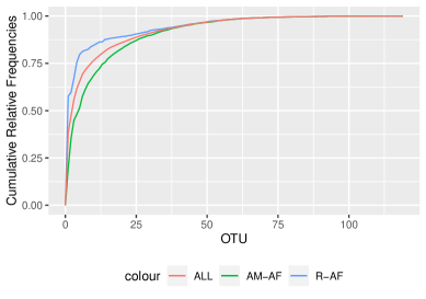
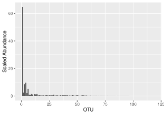
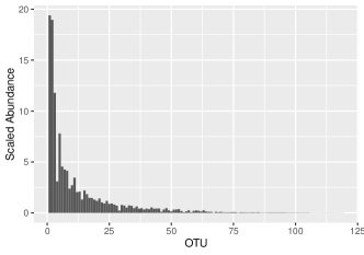
Rural-African

African-American

Figure 1: Top: Cumulative Relative Frequencies of OTU for average Rural Africans (RU), average African Americans (AA) and average of all subjects. Bottom: Histogram of OTU abundancy in RA and AA (scaled as described in the text).

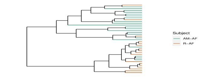
Figure 2: Agglomerative Hierarchical Clustering with Euclidean Distance and Complete method subjects using 10 OTUs with highest cross-subject variance.

Protein expression - nonparametric regression.

In a second example we analyze protein measurement data in a study of ataxia, a neurodegenerative disease. The same data is studied in Lee et al. (2021). The data measures the abundancy of $4350$ potentially disease-related proteins among two groups of subjects, one control group and one patient group. Each group includes $16$ subjects with ages between 5 and 50 years. The subjects’ ages define time for our observations. There are $T=16$ unique times $\tau_{t}$, $t=1,\ldots,T$, with one control and one patient for each unique time $\tau_{t}$. That is, $\tau$ refers to time in calendar years, and $t$ states time as an index in the list of $T$ unique time points. The data are protein activation data $y_{ij}$, $j=1,\ldots,J$, $i=1,\ldots,I$, for the $J=32$ subjects and $I=4350$ proteins. For each subject, $z_{j}$ is an indicator for being a patient ($z_{j}=1$) or control ($0$), and $t_{j}\in\{1,\ldots,T\}$ denotes the age. The inference goal is to identify proteins that are related with the disease, defined as proteins with a large difference between patients and controls in change of protein expression over age. We set up a nonparametric regression for $y_{ij}$ versus age $t_{j}$. The regression mean function is constructed using a cubic B-splines with 2 interior knots, an offset for protein $i$, and an interaction of treatment and B-spline, to allow for a difference in spline coefficients for patients versus controls. See the later discussion for more model details. In this case, the separate exchangeability assumption is made for protein-and-age specific effects $\theta_{it}$ that appears in the regression mean function.

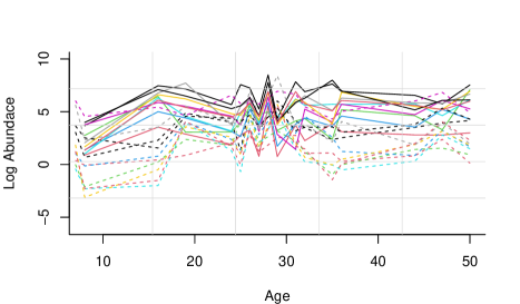
Figure 3: Randomly selected 10 proteins: log abundancy $y_{ij}$ against age $t_{j}$. Solid lines correspond to patients ($z_{j}=1$), and dotted lines indicate controls ($z_{j}=0$). Lines corresponding to the same protein share the same color.

Figure 3 shows a random subset of the data. The figure shows protein expression (on a logarithmic scale) over time for $10$ randomly selected proteins, separately for patient and control groups. The figure highlights the high level of noise in this data.

Naive method 1: Empirical difference of differences
1	Q9H6R3	Q9Y3E1	P49591	Q9NQ66-1	P01859
6	O60256-1	P10915	P10768	P53041	Q9H6U6-8
Naive method 2: separate regression for each protein
1	Q13634-1	Q9Y6U3	P04275	Q5VSL9-1	Q9NYY8
6	Q9UPU9-1	P06454-1	P24844-1	Q8WZA9	P48651

Table 1: Top 10 selected proteins using simple data summaries. Notice the lack of overlap. See the text for details.

Recall the primary inference goal of identifying proteins with the largest difference in slopes between patients versus controls. Table 1 shows the selected top 10 proteins using two simple data summaries. Let $j_{01},j_{0T},j_{11}$ and $j_{1T}$ denote the indices of four subjects, with $j_{zt}$ indicating the subject with $z_{j}=z$ and $t_{j}=t$. The first set of 10 proteins are the proteins with the largest empirical difference

$$\hat{\gamma}_{i}=\frac{y_{ij_{1T}}-y_{ij_{11}}}{T-1}-\frac{y_{ij_{0T}}-y_{ij_{01}}}{T-1},$$ (15)

that is, the 10 proteins with largest observed difference between patients and controls in change over time. One problem with $\hat{\gamma}_{i}$ is that it is based on only the 4 subjects with minimum and maximum age, and does not borrow any strength from data for subjects with ages in between, or other proteins. And both summaries ignore uncertainty of $\hat{\gamma}_{i}$. The second set of 10 proteins are the proteins with largest fitted difference, fitting for each protein two separate smoothing splines, one to all patients and a second one to all controls, and evaluating $\hat{\gamma}_{i}$ replacing the data by the fitted values $\hat{y}_{ij}$ under these smoothing splines. The second set therefore includes borrowing of strength across all subjects, but still no borrowing of strength across proteins. Note that the top 10 proteins based on these two data summaries include no overlap, highlighting again the high level of noise in these data, and the need for more principled inference and characterization of uncertainties. These observations motivate us to develop a hierarchical model to borrow strength across proteins and time, and to allow for a full description of uncertainties. The hierarchical model across subjects and proteins is set up using separate exchangeability on parameters $\bm{\theta}_{it}$. Note that in this case separate exchangeability is not on the data, but on parameters (including slope etc.) of the fitted curves. See later for details. The model includes a random partition of proteins to group proteins with similar patterns into common clusters, allowing us to identify a group of interesting proteins as the cluster with the highest cluster-specific change in protein expression over time.

4 Separate Exchangeability through Nested Partitions

4.1 Separate versus partial exchangeability

The microbiome data records frequencies $y_{ij}$ of $I=119$ OTUs $i=1,\ldots,I$, for $J=38$ subjects, $j=1,\ldots,J$. The measurement $y_{ij}$ reports the scaled abundancy of OTU $i$ in subject $j$. The main inference goal is identify subgroups $C_{k}$, $k=1,\ldots,K^{+}$, of subjects with different patterns of OTU frequencies. The subsets $C_{k}$ define a partition as $\bigcup_{k=1}^{K^{+}}C_{k}=[J]$ with $C_{k}\cap C_{k^{\prime}}=\emptyset$ for $k\neq k^{\prime}$. We refer to the $C_{k}$ as subject clusters. Alternatively we represent $C_{k}$ using cluster membership indicators $S_{j}=k$ if and only if $j\in C_{k}$.

Partially exchangeable model.

We assume mixture of normal distributions. Let $\mbox{GEM}(\alpha)$ denote a stick-breaking prior for a sequence of weights (Sethuraman, 1994). Marginally for each subject $j$ (i.e., marginalizing over other subjects, $j^{\prime}\neq j$), we assume

$$y_{ij}\mid S_{j}=k \overset{iid}{\sim}G_{k},\;i=1,2,\ldots\;$$

$$G_{k}=\sum_{\ell=1}^{\infty}w_{k\ell}N(\mu_{\ell},\sigma_{\ell}^{2})\mbox{ and }\theta_{\ell}=(\mu_{\ell},\sigma_{\ell}^{2})\overset{iid}{\sim}G_{0},~{}\bm{w}_{k}\sim\mbox{GEM}(\alpha)$$

$$p(S_{j}=k\mid\bm{\pi}) =\pi_{k}\mbox{ and }\bm{\pi}=(\pi_{1},\ldots)\sim\mbox{GEM}(\beta)$$ (16)

with independent sampling across $i=1,\ldots,I$. Marginally, for one subject $j$, the first two lines of (16) imply a Dirichlet process (DP) mixture of normal model for $y_{ij},\,i=1,2,\ldots$. That is, the marginal law for each $j$ is a DP mixture

$$y_{ij}\mid G\overset{iid}{\sim}G,~{}i=1,\ldots,I,$$

$$G=\int N(\mu,\sigma^{2})\,dF(\mu,\sigma^{2})\mbox{ and }F=\sum_{\ell}w_{k\ell}\delta_{\mu_{\ell},\sigma_{\ell}}\sim\mbox{DP}(\alpha,G_{0}).$$ (17)

We keep using notation $w_{k\ell}$ to highlight the link with (16). Here $(\mu_{\ell},\sigma_{\ell})$ are the atoms of a discrete random probability measure $F$ and $\mbox{DP}(\alpha,G_{0})$ defines a DP prior with total mass $\alpha$ and base measure $G_{0}$. See, for example, (Müller et al., 2015, Chapter 2) for a review of such DP mixture models. However, the fact that in (16) multiple subjects can share the same $G_{k}$ introduces dependence across subjects. Additionally, note that the normal moments $\theta_{\ell}=(\mu_{\ell},\sigma_{\ell}^{2})$ are indexed by $\ell$ only, implying common atoms of the $G_{k}$ across $k$. The model construction is completed by assuming that $y_{ij}$ in (16) are sampled independently also across $j$ given the vector of random probabilities. Below we will introduce a variation of this final assumption, motivated by the following observation.

The use of common atoms $(\mu_{\ell},\sigma_{\ell})$ across $G_{k}$ allows us to define clusters of observations across OTUs and subjects. This is easiest seen by replacing the mixture of normal model in the first line of (16) by a hierarchical model with latent indicators $\tilde{M}_{ij}$ as

$$p(y_{ij}\mid\tilde{M}_{ij}=\ell)=N(\mu_{\ell},\sigma_{\ell}^{2})\mbox{ and }p(\tilde{M}_{ij}=\ell\mid S_{j}=k)=w_{k\ell}.$$

Interpreting $\tilde{M}_{ij}$ as cluster (of OTUs) membership indicators, the model defines a random partition $\Psi_{j}$ of OTUs for each subject $j$ with clusters defined by $R_{j\ell}=\{(ij):\;\tilde{M}_{ij}=\ell\}$, i.e., $\Psi_{j}=\{R_{j\ell},\;\ell=1,2,\ldots\}$. In this construction subjects $j$ with shared $S_{j}=k$ share the same prior $p(\Psi_{j})$ on the partition of OTUs, implied by $y_{ij}\mid P_{j}\sim P_{j}$ with $P_{j}=G_{S_{j}}$, defining partial exchangeability as in (4), with the random partition $(S_{1},\ldots,S_{J})$ defining a dependent prior on $(P_{1},\ldots,P_{J})$. Conditional of $S_{1},\ldots,S_{J}$ the latter is characterized by only $K^{+}$ distinct $G_{k}$.

A separately exchangeable prior.

Recognizing the described construction with $\tilde{M}_{ij}$ as reducing to partial exchangeability when non-degenerate separate exchangeability is implied by the nature of the experiment, we introduce a modification. While the change is minor in terms of notation, it has major consequences for interpretation and inference as we will show later. We replace the indicators $\tilde{M}_{ij}$ by $M_{ik}$ (note the subindex _k) specific to each OTU and cluster of subjects, with otherwise unchanged marginal prior

$$p(M_{ik}=\ell)=w_{k\ell}$$ (18)

and $p(y_{ij}\mid S_{j}=\ell,M_{ik}=\ell)=N(\mu_{\ell},\sigma^{2}_{\ell})$. The assumption completes the marginal model (16) by introducing dependence of the $y_{ij}$ across $j\in C_{k}$, which is parsimoniously introduced with the $M_{ik}$ indicators. The marginal distribution (17) remains unchanged. But now the implied random partitions $\Psi_{j}$ are shared among all $j\in C_{k}$.

In practice we use an implementation using a finite Dirichlet process (Ishwaran and James, 2001) for $G_{k}$, i.e., we truncate $G_{k}$ with $L$ atoms. Similarly, we truncate the stick-breaking prior for $\pi_{k}$ at a fixed number of $K$ atoms. For later reference we state the joint probability model conditional on $K$ and $L$ is

$$p(y_{1:I,1:J},\bm{S},\bm{M},\bm{\pi},\bm{w},\mid K,L)=\prod_{j=1}^{J}\prod_{i=1}^{I}p(y_{ij}\mid\mu_{M_{i,S_{j}}},\sigma^{2}_{M_{i,S_{j}}})\\ \times\prod_{j=1}^{J}\pi_{S_{j}}\left\{\prod_{k=1}^{K}\prod_{i=1}^{I}w_{M_{ik},k}\right\}\;p(\bm{\pi})\,\prod_{k=1}^{K}p(\bm{w}_{k})\,\prod_{\ell=1}^{L}p(\mu_{\ell},\sigma^{2}_{\ell})$$ (19)

with $p(\bm{\pi})=p(\pi_{1},\ldots,\pi_{K})=\mbox{GEM}(\beta)$ and $p(\bm{w}_{k})=p(w_{k1},\ldots,w_{kL})=\mbox{GEM}(\alpha)$ being finite stick breaking priors, and $p(\mu_{\ell},\sigma^{2}_{\ell})$ chosen to be conditionally conjugate for the sampling model $p(y_{ij}\mid\mu_{\ell},\sigma^{2}_{\ell})$.

In summary, we have introduced separate exchangeability for $y_{ij}$ by defining (i) a random partition $\gamma=\{C_{1},\ldots,C_{K^{+}}\}$ of columns, corresponding to the cluster membership indicators $S_{j}$, and (ii) nested within column clusters $C_{k}$, a nested partition $\Psi_{j}=\{R_{j1},\ldots,R_{jL}\}$ of rows, represented by cluster membership indicators $M_{ik}$. In contrast, a model under which $j\in C_{k}$ only share the prior $p(\Psi_{j})$ on the nested partition reduces to the special case of partial exchangeability. The model remains invariant under arbitrary permutation of the row (OTU) labels in any column (subject). Without the reference to separate exchangeability a similar construction with nested partitions was also used in Lee et al. (2013). The construction of the nested partition is identical, but there is no notion of common atoms to allow for clusters of observations across column clusters.

Finally, to highlight the nature of the model as being separately exchangeable with respect to OTUs and subjects we exhibit the explicit Aldous-Hoover representation (11), still conditional on hyperparameters. We show separate exchangeability conditional on $\phi=(\bm{\pi},\bm{w})$ by matching variables with the arguments in (11) as follows: $\eta_{j}=S_{j}$, $\xi_{i}=(M_{ki},k=1,\ldots,K)$, $\theta=(\bm{\mu},\bm{\sigma})$, and $p(x_{ij}\mid\theta,\xi_{i},\eta_{j})=N(\mu_{\ell},\sigma^{2}_{\ell})$ with $\ell=M_{S_{j}i}$. Here we used that (11) allowed conditioning on additional hyperparameters, in this case $\phi$.

4.2 Results

Posterior simulation is implemented as a straightforward Gibbs sampling algorithm. All required complete conditional distributions follow easily from the joint probability model (19). Posterior Monte Carlo simulation is followed by a posterior summary of the random partition using the approach of Dahl (2006) to minimize Binder loss, using the algorithm in Dahl et al. (2021). We estimate three clusters of subjects, $C_{1},C_{2},C_{3}$. We show the three subject clusters in Figure 4 by plotting cumulative frequencies of OTUs. We sort all OTUs by overall abundancy across subjects. For each cluster of subjects, we collect all subjects $j$ and plot cumulative (observed) frequencies.

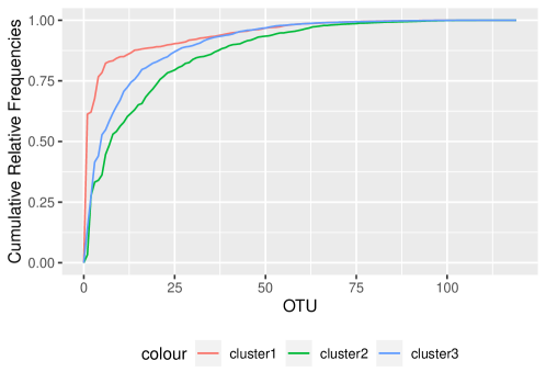
Figure 4: Cumulative Relative Frequencies of OTU in the subject clusters $C_{k}$, $k=1,2,3$, of subjects.

Figure 5 summarizes the nested partition of OTUs, nested within the three subject clusters. The three panels correspond to subject clusters $k=1,2$ and $3$. For each subject cluster, the figure shows the estimated co-clustering probabilities of OTUs, i.e., $p^{k}_{ii^{\prime}}=p(M_{ik}=M_{i^{\prime}k}\mid\bm{y},\bm{S})$ for each pair $(i,i^{\prime})$ of OTUs. As usual for heatmaps, the OTUs are sorted for a better display, to highlight the clusters.

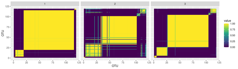
Figure 5: OTU co-clustering probability under each subject cluster of subjects. In each block, OTU are ordered by their cluster assignment.

Figure 6 shows the same nested partitions, but now by showing the data $y_{ij}$ arranged by subject clusters. In each panel OTUs are sorted by observational clusters. That is, each plot shows the data corresponding to $j\in S_{k}$, for $k=1,2$ and $3$. The subjects $j\in C_{k}$ are on the x-axis. The OTUs are on the y-axis, arranged by the estimated observational clusters. The patterns in $y_{ij}$ echo the clusters shown in the previous plot.

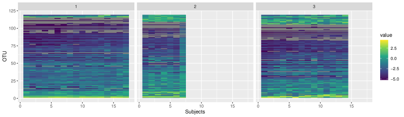
Figure 6: Heatmap of column scaled y in log scale for each subject clusters of subjects. OTU is sorted by each cluster specific OTU cluster assignment.

Inference as in Figure 5 or 6 is not meaningfully possible under partial exchangeability, since the nested partitions $\rho_{j}=(R_{j\ell},\ell=1,\ldots,L)$ are not shared across $j\in C_{k}$. In other words, consider for example two subjects $j=1$ and $j=2$. Assume for subject 1 we record two OTUs $a$ and $b$ co-cluster in a cluster with high frequency, whereas for subject 2 OTUs $c$ and $d$ cluster together. Under partial exchangeability $j=1$ and $2$ might be placed in the same cluster $C_{k}$ although the different OTUs might be linked to entirely different diets.

5 Nonparametric Regression

5.1 Separate exchangeability in an ANOVA DDP model

ANOVA DDP.

In this example we set up a separately exchangeable model as an implementation of the popular dependent Dirichlet process (DDP), by means of introducing the symmetric structure in the prior for the atoms in a Dirichlet process (DP) random measure over subjects and time. In this example, the separate exchangeability assumption is not on the observed data (protein expression over time and two different conditions). Instead we set up a separately exchangeable prior for the linear model parameters in a statement of the DDP as a DP mixture of linear models. The actual construction is very simple. We achieve separate exchangeability by setting up additive structure with terms specific to proteins $i$ and time $t$.

The DDP is a predictor-dependent extension of DP mixtures first proposed by MacEachern (1999, 2000). It defines a family of random probability measures $\mathcal{F}=\{F_{x},\;x\in X\}$, where the random distributions $F_{x}$ are indexed by covariates $x$ and each $F_{x}$ marginally follows a DP prior as in (17). The desired dependence of $F_{x}$ across $x$ is achieved by writing the atoms or the weights of the DP random measure $F_{x}$ as functions of covariates (Quintana et al., 2020). The simplest version of the DDP arises when only the atoms of $F_{x}$ vary over $x$ (common weights DDP) and are specified as a linear function of $x$. This defines the linear dependent DP (LDDP) or ANOVA DDP (De Iorio et al., 2004). The model can be written as a DP mixture of linear models, that is, as a mixture with respect to some (or all) linear model parameters, and a DP prior on the mixing measure. See below for a specific example.

The DDP naturally implements partially exchangeable structure if it is assumed as de Finetti measure in (4). Consider data $y_{ij}$, assuming $p(y_{ij}\mid\mathcal{F})=\int p(y_{ij}\mid\theta)\;dF_{j}(\theta)$, typically using the additional convolution with a density kernel $p(y_{ij}\mid\theta)$ to construct a continuous sampling model, if desired. A similar situation arises when data $y_{i}$ is observed with a categorical covariate $w_{i}\in\{1,\ldots,J\}$ and $p(y_{i}\mid w_{i}=j,\mathcal{F})=\int p(y_{ij}\mid\theta)\;dF_{j}(\theta)$. In either case, a DDP prior on $\mathcal{F}=(F_{j},j=1,\ldots,J)$ implements a partially exchangeable model for the observable data $y_{ij}$, or $y_{i}$ grouped by $w_{i}$, respectively. However, if the experimental context calls for separately exchangeable structure with respect to $i$ and $j$, appropriate model variations are called for. We introduce one next, where the separately exchangeable structure is on the parameters $\theta$ in (a variation of) the DP mixture representation.

A separately exchangeable ANOVA DDP.

To state the specific model we need some more notation. Recall the notation set up in Section 3, with $y_{ij}$ denoting the abundancy of protein $i$ in subject $j$, and $t_{j}$ and $z_{j}$ denoting subject-specific age and condition. We use cubic B-splines with two internal nodes to represent protein expression over a grid of $T=16$ time points, $\tau_{t}$, $t=1,\ldots,T$. The linear model parameters in the ANOVA DDP model include coefficients for the B-spline basis functions to represent protein expression over time for controls, plus an additional equal number of coefficients for the same basis functions to represent an offset for protein expression for patients. More specifically, let $\bm{x}_{j}\in\Re^{12}$ denote a design vector for subject $j$, with $(x_{j1},\ldots,x_{j6})$ being 6 spline basis functions evaluated at time $t_{j}$, and $(x_{j7},\ldots,x_{j,12})=z_{j}(x_{j1},\ldots,x_{j,6})$ representing an offset for patients ($z_{j}=1$). That is, linear model coefficients for $(x_{j1},\ldots,x_{j6})$ model protein expression over time for controls ($z_{j}=0$), while the coefficients for $(x_{j7},\ldots,x_{j,12})$ represent an additional offset for patients ($z_{j}=1$) in protein expression over time.

Let $\bm{y}_{i}=(y_{ij},\;j=1,\ldots,J)$ denote all data for protein $i$. We assume an ANOVA DDP model, written as DP mixture

$$f(\bm{y}_{i}\mid G,\bm{\alpha},\bm{\delta})=\int\left\{\prod_{j=1}^{J}N(y_{ij};\alpha_{i}+\delta_{t_{j}}+\bm{x}_{j}^{\prime}\bm{\beta}_{i},\sigma^{2}_{i})\;\right\}dG(\bm{\beta}_{i},\sigma_{i}^{2})),$$ (20)

with a DP prior for $G=\sum_{h}\pi_{h}\delta_{\tilde{\beta}_{h},\tilde{\sigma}_{h}}$, $G\sim\mbox{DP}(\xi,G_{0}).$ Here $\alpha_{i}$ are protein-specific offsets and $\delta_{t}$ are offsets for each of the unique time points, $t=1,\ldots,16$. We use a finite DP, $G\sim\mbox{DP}_{H}(\xi,G_{0})$, truncated at $H=25$ (Ishwaran and James, 2001), with total mass parameter $\xi$ and $G_{0}$ defined by $\bm{\beta}_{h}\sim N(\bm{\beta}_{0},\sigma_{\beta 0}I)$ and $\sigma^{2}_{h}\sim\mbox{InvGa}(a_{0},b_{0})$. We complete the prior specification with $\delta_{t}\sim N(\zeta,\omega)$ and $\alpha_{i}\sim N(\mu_{0},\sigma_{0}^{2})$. Here, $(\xi,\bm{\beta}_{0},\sigma_{\beta 0},a_{0},b_{0},\mu_{0},\sigma^{2}_{0},\zeta_{0},\omega_{0})$ are fixed hyperparameters. See Appendix B for specific values.

Note that the linear model is over-parametrized. For example, we do not restrict the cubic splines to zero average over all (two) subjects observed at the same time $t_{j}=t$, implying confounding of the intercept with $\delta_{t}$. However, recall that the inference target is the difference in slope between patient and control for a given protein, which is not affected by this over-parametrization.

The regression model is set up to allow straightforward inference on the protein-specific difference in slope for patients versus controls. As in (15), let again $j_{01},j_{0T},j_{10},j_{1T}$ denote indices of subjects with $(z_{j},t_{j})=(0,1),(0,T),(1,1)$ and $(1,T)$, respectively. Then keeping in mind that $\bm{x}_{j_{1T}}$ and $\bm{x}_{j_{0T}}$ differ only in the last 6 elements (and ignoring scaling by a constant $1/(T-1)$),

$$\gamma_{i}=[(\bm{x}_{j_{1T}}-\bm{x}_{j_{11}})-(\bm{x}_{j_{0T}}-\bm{x}_{j_{01}})]\bm{\beta}_{i}=(\bm{x}_{j_{1T},7:12}-\bm{x}_{j_{11},7:12})\bm{\beta}_{i,7:12}$$ (21)

represents the desired difference in slope between patients and controls. Posterior inference on $\gamma_{i}$ implements the desired model-based inference on the difference of slopes with borrowing of strength across proteins and subjects.

Let $\bm{\theta}_{it}=(\alpha_{i},\delta_{t},\bm{\beta}_{i},\sigma^{2}_{i})$ denote the parameters that index the regression model for protein $i$ at time $t$. By construction the prior probability model on $\bm{\theta}_{it}$ is separately exchangeable, as it is invariant with respect to separate permutations $\pi$ of protein indices and $\pi^{\prime}$ of age:

$$p(\bm{\theta}_{1:I,1:T})=p(\bm{\theta}_{\pi(1:I),\pi^{\prime}(1:T)}).$$

Note that $\bm{\beta}_{i}$ represents the mean function for patient $i$ as coefficients for the spline basis (valid for any $t$). Only in (20) this mean function is evaluated for $t=t_{j}$ and $x=x_{j}$. In particular, separate exchangeability is assumed for the mean function parameters, not for the fitted values or the data. The model is separately exchangeable by construction. Alternatively one can trivially match the variables with the arguments in (11), $\xi_{i}=(\alpha_{i},\bm{\beta}_{i},\sigma_{i})$ and $\eta_{t}=\delta_{t}$.

5.2 Posterior Inference

MCMC posterior simulation.

Posterior simulation under the proposed ANOVA DDP (or DDP of splines) model for protein expression is straightforward. We used the R function bs from the package splines to evaluate the spline basis functions for $\bm{x}_{j}$. The transition probabilities are detailed in Algorithm 1 in the appendix.

For the statement of the detail transition probabilities in Algorithm 1 it is useful to replace the mixture model (20) by an equivalent hierarchical model

$$y_{ij}\mid s_{i}=h\sim N(\alpha_{i}+\delta_{t_{j}}+\bm{x}_{j}^{\prime}\tilde{\bm{\beta}}_{h},\tilde{\sigma}^{2}_{h})$$ (22)

with $p(s_{i}=h)=\pi_{h}$. Recall that $(\tilde{\bm{\beta}}_{h},\tilde{\sigma}_{h})$ are the atoms of the random mixing measure $G$ in (20), and that we use a finite DP truncated at $H$ atoms. Interpreting $s_{i}$ as cluster membership indicators defines inference on a random partition of proteins. Let then $C_{h}=\{i:\;s_{i}=h\}$ denote cluster $h$ defined by $s_{i}$, and let $n_{h}=|C_{h}|$. Note that in this notation we allow for empty clusters that arise when an atom $(\tilde{\bm{\beta}}_{h},\tilde{\sigma}_{h})$ is not linked with any observation, i.e., $C_{i}=\emptyset$ and $n_{h}=0$. Using this notation, see Algorithm 1 in Appendix B for a description of MCMC posterior simulation.

We are mainly interested in two posterior summaries, a partition of proteins by different patterns of protein expression over time, and identification of the proteins with the highest rank in $|\gamma_{i}|$ (the difference in slope between patients and control). The latter proteins are the ones that are most likely linked with ataxia.

We start by identifying the MAP estimate $K^{*}$ for the number of clusters ${K^{+}}=\sum_{h}1(n_{h}>0)$ in (22), and then follow the approach of Dahl (2006) to report a posterior summary of the random partition of proteins. Let $s^{*}$ denote the reported partition. Conditional on $s^{*}$, we then generate a posterior Monte Carlo sample for $\tilde{\beta}_{h}$ for each cluster to obtain (conditional) posterior mean and variance for the cluster-specific $\bm{\tilde{\beta}}_{h}$. We did not encounter problems related to label-switching in the actual implementation - in general one might need to account for possible label-switching.

Ranking proteins.

The main inference target is to identify proteins with the most significant difference between time profiles for patients versus controls, suggesting such proteins are the most likely to be linked with ataxia.

We therefore focus on the difference (across conditions) in differences (over age) of mean protein expression, defined as $\gamma_{i}$ in (21). We evaluate the posterior mean $E(\gamma_{i}\mid\bm{y})$ using Rao-Blackwellization, that is, as Monte Carlo average of conditional expectations $\bar{\gamma}_{i}=\frac{1}{M}\sum_{m}E(\gamma_{i}\mid\theta^{(m)-},\bm{y})$, where $\theta^{(m)-}$ are all parameters in the $m$-th posterior Monte Carlo sample, excluding $\bm{\beta}$. Note that $\gamma_{i}$ is a deterministic function of the cluster-specific $\tilde{\beta}_{h}$ when $s_{i}=h$. Let $\tilde{\gamma}_{h}$ denote the cluster-specific estimate. Conditioning on $s^{\star}$ we can then identify the set of proteins with the largest average change.

Alternatively, we can cast the problem of identifying interesting proteins as a problem of ranking, and more specifically, one of estimating a certain quantile, to report the most promising $100(1-c)\%$ proteins. Here $c$ is chosen by the investigator. Choice of $c$ should reflect the effort and capacity to further investigate selected proteins. We then formalize the problem of reporting promising proteins as the problem of identifying the proteins with $|\gamma_{i}|$ in the top $(1-c)$ percentile of $|\gamma_{i}|$ values. The problem of ranking experimental units in a hierarchical model and reporting the top $(1-c)$ percentile is discussed in Lin et al. (2004) who cast it as a Bayesian decision problem. Let

$$R_{i}=\mbox{rank}(\gamma_{i})=\sum_{i^{\prime}=1}^{I}I(|\gamma_{i}|\geq|\gamma_{i^{\prime}}|),$$

denote the true ranks, with $R_{i}=1$ for the smallest $|\gamma_{i}|$ and $R_{i}=I$ for the largest $|\gamma_{i}|$. Alternatively we use $P_{i}=R_{i}/(I+1)$ to report the quantile, or the percentile $100\,P_{i}\%$. One of the loss functions that Lin et al. (2004) consider is a 0-1 loss aimed at identifying the top $100(1-c)\%$ units, i.e., the $c-$quantile. Let $\widehat{R}_{i}$ denote the estimated rank for unit $i$, and $\widehat{P}_{i}=\widehat{R}_{i}/(I+1)$. The following loss function penalizes the number of misclassifications in the top $c$ quantile, including the number of proteins that are falsely reported (false positives) plus those that are failed to be reported (false negatives).

$$L_{0/1}(c)=\frac{1}{I}\{\text{\# misclassifications}\}=\frac{1}{I}\left\{\sum_{i=1}^{I}\mbox{AB}(c,P_{i},\widehat{P}_{i})+\mbox{BA}(c,P_{i},\widehat{P}_{i})\right\}$$

where AB and BA are penalties for the two types of misclassifications,

$$AB(c,P,\widehat{P})=\bm{1}(P>c,\widehat{P}<c)=\bm{1}(R>c(I+1),\widehat{R}<c(I+1),$$

$$BA(c,P,\widehat{P})=\bm{1}(P<c,\widehat{P}>c)=\bm{1}(R<c(I+1),\widehat{R}>c(I+1),$$

Lin et al. (2004) show that $L_{0,1}(c)$ is optimized by $\widehat{R}_{i}=R^{\star}_{i}$ with

$$R^{\star}_{i}(c)=\mbox{rank}\{p(P_{i}>c\mid\bm{y})\},$$ (23)

or $P^{\star}_{i}=R^{\star}_{i}/(I+1)$.

5.3 Simulations

We set up a simulation with $J=20$ subjects and $I=100$ proteins. The simulation does not include a split into patients and control (think of the data as already reporting the difference of patient and control). We generate $t_{j}\sim\mbox{Unif}\,(0,1)$ (equivalent to age in the actual study), a hypothetical partition of proteins with cluster membership indicators $s_{i}\in\{1,2,3\}$ using $p(s_{i}=h)=\pi_{h}$, $\bm{\pi}=(0.25,0.3,0.45)$. We set up protein-specific offsets $\alpha_{i}$ using shared common values for all proteins in a cluster, i.e., $\alpha_{i}=\tilde{\alpha}_{s_{i}}$ with $(\tilde{\alpha}_{1},\tilde{\alpha}_{2},\tilde{\alpha}_{3})=(0,-3,1)$, and patient-specific offsets $\delta_{j}\sim N(0,0.1)$. To mimic the actual data, we manually modify some $\delta_{j}$ to create similar patterns as in the data (see Figure 8b). Using these parameters we set up a simulation truth

$$y_{ij}=\begin{cases}\alpha_{i}+2t_{j}+3t_{j}^{3}+\delta_{j}+\epsilon_{ij},&s_{i}=1\\ \alpha_{i}-2t_{j}+t_{j}^{3}+\delta_{j}+\epsilon_{ij},&s_{i}=2\\ \alpha_{i}+t_{j}-3t_{j}^{3}+\delta_{j}+\epsilon_{ij},&s_{i}=3\end{cases}$$

with $\epsilon_{ij}\sim N(0,\sigma)$ and $\sigma=0.2,0.5,1$ for $s_{i}=1,2,3$, respectively. See Figure 8b (black lines) for the mean functions for proteins in the three clusters under the simulation truth. Under this simulation truth, the proteins in cluster $2$ are those with largest overall slope. Figure 7 shows $20$ randomly selected $y_{i}$ versus age $t$, in the simulation (left panel) and in the real data (right panel).

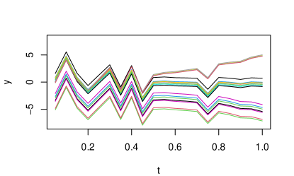
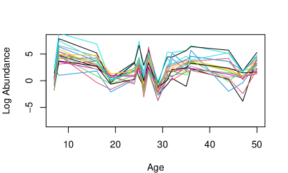
Simulation	Data

Figure 7: Left: $20$ randomly selected $y_{i}$ from simulation versus age $t$, each color indicates a different $y_{i}$. Right: the mean log abundancy difference between patient and control in $20$ randomly selected proteins from data.

MCMC posterior simulation converges after $3000$ iterations. As before, let $n_{h}=|C_{h}|$, and let $K^{+}=\sum_{h=1}^{H}I(n_{h}>0)$ denote the number of non-empty clusters. Figure 8a shows a histogram of the posterior distribution $p(K^{+}\mid\bm{y})$. The posterior mode $K^{\star}=3$ recovers the simulation truth, with little posterior uncertainty. We then evaluate the earlier described point estimate $s^{\star}$ for the posterior random partition. Conditioning on $s^{\star}$ we continue to simulate MCMC transitions to evaluate conditional posterior means for $\bm{\tilde{\beta}}_{h}$, $\alpha_{i}$ and $\delta_{t}$ in the analysis model (20).

Let $\bar{\delta}_{t}=E(\delta_{t}\mid s^{\star},\bm{y})$, $\bm{\bar{\beta}}_{h}=E(\bm{\tilde{\beta}}_{h}\mid s^{\star},\bm{y})$ and $\bar{\alpha}_{i}=E(\alpha_{i}\mid s^{\star},\bm{y})$ denote the conditional posterior means. All posterior means are evaluated numerically as Monte Carlo sample averages. Also, let $\alpha^{\star}_{h}=\frac{1}{n_{h}}\sum_{i\in C_{h}}\bar{\alpha}_{i}$. For a data point $y_{ij}$, let $t=t_{j}$ and $h=s^{\star}_{i}$. Then $\widehat{y}_{ht}=\alpha^{\star}_{h}+\bar{\delta}_{t}+\bm{x}_{j}^{\prime}\bm{\bar{\beta}}_{h}$ are the posterior fitted values for $y_{ij}$. Figure 8(b) shows the posterior fitted values $\widehat{y}_{hzt}$ and pointwise one-standard deviation intervals. The estimates closely track the true mean profiles.

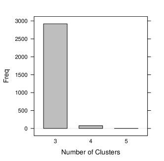
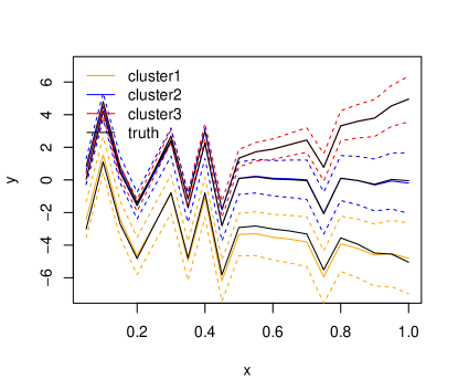
(a)

(b)

Figure 8: (a) Histogram of $p(K^{+}\mid\bm{y})$ in the simulation experiment. The simulation truth is ${K^{+}}=3$. (b) Prediction $\widehat{y}_{ht}$ (solid black line) and simulation truth (solid color line) for each cluster in the simulation experiment versus age $t$. Dotted lines indicate pointwise one standard deviation standard errors.

These simulation results indicate that with moderate sample sizes as in the actual study, and noise levels comparable to the data, inference could reliably estimate protein expression over time. The a posteriori identification of the proteins with the largest change over time perfectly recovers the simulation truth in this example. The assignment $s^{\star}$ includes no misclassification for any of the 100 proteins.

5.4 Results

We implement inference under the proposed DDP model with the separately exchangeable prior. We find the following eleven clusters for the $4350$ proteins. For each cluster, we separately plot the cluster predicted protein abundancy $\widehat{\bm{y}}_{h}=(\widehat{y}_{ht},\;t=1,\ldots,T)$ for patients (solid) versus control (dashed). For comparison we show corresponding averages of protein expression, averaging the data $y_{ij}$ across all patients (dotted) and controls (dash-dotted) for each estimated cluster (under $s^{\star}$). The predicted mean protein abundancy for each cluster $h$ is computed as before, as $\widehat{y}_{hzt}=\bar{\delta}_{t}+\bm{x}_{j_{zt}}^{\prime}\bar{\beta}_{h}+\alpha^{\star}_{h},$ for a data point $y_{ij}$ with $s^{\star}_{i}=h$, $t_{j}=t$ and $z_{j}=z$, and the cluster-specific posterior means $\bar{\beta}_{h}$ and $\alpha^{\star}$ defined as before.

In Figure 9, we see noticeably different trajectories for patients and controls, except for cluster $k=3$ (in panel (c)). The figure also indicates $R^{2}$ (coefficient of determination) as an indication of model fit for each cluster, with an average $R^{2}$ of $0.70$ ($0.075$ empirical standard deviation) across the $K^{+}$ clusters. For an additional goodness of fit assessment we use a model fit diagnostic proposed by Johnson (2004). For each iteration, we randomly select a subject $j$ and protein $i$, calculate the fitted value $\widehat{y}_{ij}^{(m)}=\widehat{y}_{hzt}$ using currently imputed parameters, including the random partition $\bm{s}$, and form the residual $z_{ij}=y_{ij}-\widehat{y}_{ij}^{(m)}$. Figure  10 shows a normal q-q plot of the residuals $z_{ij}$, dropping an initial burn-in and thinning out iterations. The approximately $45$ degree line indicates no evidence against model fit.

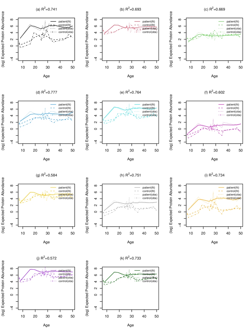
Figure 9: Predicted protein abundancy $\widehat{y}_{hzt}$ in cluster $h$ versus age $t$ for patients ($z=1$, solid) and controls ($z=0$, dashed) versus age $t$. For comparison, the dotted and dash-dotted line plots the average over all patients in the same cluster (under $s^{\star}$) under condition $z$ at time $t$.

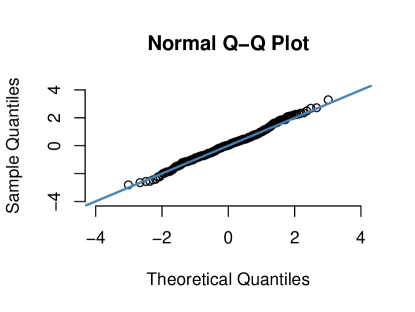
Figure 10: Normal Q-Q plot of residuals.

Evaluating the posterior rank summary (23) we find top $100$ ($=2.5\%$) ranked proteins, with highest $|\gamma_{i}|$, i.e., (absolute) difference of slopes between patients and controls. Table 2 shows the top 20 of these.

1	Q15149-8	Q13813-2	Q13813-3	Q01082-1	O15020
6	Q00610-1	Q14643-5	Q01484	P49327	P46821
11	P14136	Q8NF91	P35580-4	P14136-3	Q05193-3
16	Q05193-5	P61764-2	P46459	P61764	P07900-2

Table 2: Top 20 Ranked Proteins with highest posterior $|\gamma_{i}|$

6 Discussion

We have argued for the use of separate exchangeability as a modeling principle, especially for nonparametric Bayesian models. The main arguments are that (i) in many cases separate exchangeability is more faithfully representing the experimental setup than, say, partial exchangeability; and (ii) some summaries of interest (related to the identity of the experimental units) cannot even be stated without introducing separate exchangeability. An example for the latter are shared nested partitions of rows across different columns in a data matrix. In a wider context, the discussion shows that careful considerations of the experimental setup often leads to more specific symmetry assumptions than omnibus exchangeability or partial exchangeability.

In many cases separately exchangeable probability models will serve a tractable submodel of a larger, encompassing inference model as we did in Section 5.1.

Finally, recall that the proposed separately exchangeable BNP model in the first example can be rephrased in terms of dependent random partition models that exploit the random partitions induced by the ties of Dirichlet processes. In this context, an interesting future related research is to study the learning mechanisms that arise from similar composition of Gibbs-type priors (Gnedin and Pitman, 2006; De Blasi et al., 2013) that preserve analytical and computational tractability of the random partition law.

Appendix A: Proofs

We include a brief proof of (5).

Claim:

Infinite partial exchangeability (4) entails

$$\mbox{Corr}(x_{ij},x_{i^{\prime}j})\geq\mbox{Corr}(x_{ij},x_{i^{\prime}j^{\prime}})\quad j\neq j^{\prime},\,\ i\neq i^{\prime}.$$ (24)

Proof.

We define $U_{ij}\coloneqq x_{ij}/\mbox{Var}(x_{ij})$ such that $\mbox{Cov}(U_{ij},U_{i^{\prime}j})=\mbox{Corr}(x_{ij},x_{i^{\prime}j})$. By de Finetti’s theorem (4) and law of total covariance

$$\mbox{Cov}(U_{ij},U_{i^{\prime}j})=0+\mbox{Cov}\{\mbox{E}(U_{ij}\mid P_{j})\mbox{E}(U_{i^{\prime}j}\mid P_{j})\}$$

$$\geq 0+\mbox{Cov}\{\mbox{E}(U_{ij}\mid P_{j})\mbox{E}(U_{i^{\prime}j^{\prime}}\mid P_{j^{\prime}})\}=\mbox{Cov}(U_{ij},U_{i^{\prime}j^{\prime}}),$$

∎

Considering a trivial example with $>$ in (24) proves the claim in (5).

Appendix B: Algorithm 1

Algorithm 1 below states the transition probabilities for posterior simulation in model (20). The description makes use of the following notation. Let $\bm{X}$ denote a $(J\times 12)$ design matrix with $\bm{x}_{j}$ in row $j$. the following quantities are used in the description of Algorithm 1. We use a notational convention of marking quantities that are cluster-specific with a tilde, as in $(\tilde{\beta}_{h},\tilde{\sigma}_{h})$, etc. Let then $\tilde{\bm{y}}_{h},\tilde{\bm{X}}_{h}$ and $\tilde{\bm{\delta}}_{h}$ denote $y_{ij}$, $\bm{x}_{j}$ and $\delta_{t}$ arranged by clusters. That is, $\tilde{\bm{y}}$ is a $(n_{h}J\times 1)$ vector stacking $\bm{y}_{i}$ for all $i\in C_{h}$ as $\tilde{\bm{y}}_{h}=(y_{ij},\;i\in C_{H};\;j=1,\ldots,J)$; $\tilde{\bm{X}}$ is an $(n_{h}J\times 12)$ matrix with $\bm{X}$ stacked $n_{h}$ times on top of each other; and $\tilde{\bm{\delta}}_{h}$ is a $(n_{h}J\times 1)$ vector that concatenates $n_{h}$ copies of $\bm{\delta}=(\delta_{t_{1}},\ldots,\delta_{t_{J}})$.

Priors: We fixed hyperparameters: $\xi=1$, $\bm{\beta}_{0}=(0,0,\ldots,0)$, $\sigma_{\beta 0}=1$,$a_{0}=1$, $b_{0}=1$, $\zeta_{0}=0$, $\omega_{0}=0.01$, $\mu_{0}=3$, $\sigma_{0}^{2}=5$. Also, let $\bm{\Sigma}_{0}=\sigma_{\beta 0}^{2}I$.

[4pt] for 1:M  do

       1. For each protein $i$, sample

$$P(s_{i}=h\mid\cdot)\propto\pi_{h}\prod_{j=1}^{J}N(y_{ij};\alpha_{i}+\bm{x}_{j}^{\prime}\tilde{\beta}_{h}+\delta_{t_{j}},\tilde{\sigma}_{h}^{2})$$

2. Update $V_{h}$, $h=1,\ldots,H-1$, keeping in mind that $V_{H}=1$ is fixed:

$$V_{h}\mid\cdot \sim\mbox{Be}(1+n_{h},\xi+\sum_{\ell=h+1}^{H}n_{\ell}),\;h=1,\ldots,H-1$$

and set $\pi_{h}=V_{h}\prod_{\ell<h}(1-V_{\ell})$, $h=1,\ldots,H$.

      3. Update $\tilde{\bm{\beta}}_{h}$ and $\tilde{\sigma}^{2}_{h}$: Recall the definition of $\tilde{\bm{y}}_{h},\tilde{\bm{X}}_{h}$ and $\tilde{\bm{\delta}}_{h}$ as cluster-specific combined vectors and matrices. See the text for a detailed definition.

$$\tilde{\bm{\beta}}_{h}\mid\cdot \sim N(\bm{\tilde{\mu}}_{h},\bm{\tilde{\Sigma}}_{h}),$$

$$\bm{\tilde{\mu}}_{h}=\bm{\tilde{\Sigma}}_{h}\left\{\tilde{\bm{X}}_{h}^{T}\bm{\Sigma}_{h}^{-1}(\tilde{\bm{y}}_{h}-\tilde{\bm{\alpha}}_{h}-\tilde{\bm{\delta}}_{h})+\bm{\Sigma}_{0}^{-1}\bm{\beta}_{0}\right\},$$

$$\bm{\tilde{\Sigma}}_{h}=(\bm{\Sigma}_{0}^{-1}+\tilde{\bm{X}}_{h}^{T}\bm{\Sigma}_{h}^{-1}\tilde{\bm{X}}_{h})^{-1}\mbox{ and }\bm{\Sigma}_{h}=\mathrm{Diag}_{J\times n_{h}}(\tilde{\sigma}_{h}^{2}),$$

$$\tilde{\sigma}^{2}_{h}\mid\cdot \sim \mbox{InvGa}(a_{h},b_{h})$$

$$a_{h}=a_{0}+\frac{n_{h}\times J}{2}\mbox{ and }b_{h}=b_{0}+\frac{\sum_{i\in C_{h}}\sum_{j=1}^{J}(y_{ij}-m_{ij})^{2}}{2}$$

$$m_{ij}=\alpha_{i}+\bm{x}_{j}^{\prime}\tilde{\beta}_{h}-\delta_{t_{j}}$$

      4. Update age-specific effect $\delta_{t}$. Let $m_{t}=\sum_{j=1}^{J}\bm{1}(t_{j}=t)$. Sample

$$\delta_{t}\mid\cdot \sim N(m_{t},V_{t})$$

$$1/V_{t}=1/\omega^{2}+\sum_{j:\;t_{j}=t}\sum_{i=1}^{I}1/\sigma_{s_{i}}^{2}$$

$$m_{t}=V_{t}\left(\frac{\zeta}{\omega^{2}}+\frac{\sum_{j:\,t_{j}=t}\sum_{i=1}^{I}(y_{ij}-\bm{x}_{j}^{\prime}\tilde{\beta}_{s_{i}}-\alpha_{i})^{2}}{\tilde{\sigma}_{s_{i}}^{2}}\right)$$

      4. Update protein-specific intercept $\alpha_{i}$. Sample

$$\alpha_{i}\mid\cdot \sim N\left(\frac{\mu_{0}/\sigma_{0}^{2}+\sum_{j=1}^{J}\sum_{i=1}^{I}(y_{ij}-\bm{x}_{j}^{\prime}\tilde{\bm{\beta}}_{s_{j}}-\delta_{t_{j}})^{2}/\tilde{\sigma}_{s_{j}}^{2}}{1/\sigma_{0}^{2}+J/\sigma_{s_{i}}^{2}},\left(1/\sigma_{0}^{2}+J/\tilde{\sigma}_{s_{i}}^{2}\right)^{-1}\right).$$

end for

Algorithm 1 MCMC algorithm for posterior inference

References

- Aldous (1981) Aldous, D. J. (1981). Representations for partially exchangeable arrays of random variables. J. Multivar. Anal. 11(4), 581–598.
- Aldous (1985) Aldous, D. J. (1985). Exchangeability and related topics. In École d’Été de Probabilités de Saint-Flour XIII—1983, pp. 1–198. Springer.
- Bernardo and Smith (2009) Bernardo, J. M. and A. F. Smith (2009). Bayesian Theory, Volume 405. John Wiley & Sons.
- Cifarelli and Regazzini (1978) Cifarelli, D. and E. Regazzini (1978). Nonparametric statistical problems under partial exchangeability: The role of associative means. Quaderni Istituto Matematica Finanziaria, Turin.
- Dahl (2006) Dahl, D. B. (2006). Model-based clustering for expression data via a Dirichlet process mixture model. In M. Vannucci, K.-A. Do, and P. Müller (Eds.), Bayesian Inference for Gene Expression and Proteomics. Cambridge Univ. Press.
- Dahl et al. (2021) Dahl, D. B., D. J. Johnson, and P. Müller (2021). Search algorithms and loss functions for Bayesian clustering. Preprint arXiv: 2105.04451.
- De Blasi et al. (2013) De Blasi, P., S. Favaro, A. Lijoi, R. H. Mena, I. Prünster, and M. Ruggiero (2013). Are Gibbs-type priors the most natural generalization of the Dirichlet process? IEEE Trans. Pattern Anal. Mach. Intell. 37(2), 212–229.
- De Iorio et al. (2004) De Iorio, M., P. Müller, G. L. Rosner, and S. N. MacEachern (2004). An ANOVA model for dependent random measures. J. Am. Stat. Assoc. 99(465), 205–215.
- Denti et al. (2021) Denti, F., F. Camerlenghi, M. Guindani, and A. Mira (2021). A common atom model for the Bayesian nonparametric analysis of nested data. J. Am. Stat. Assoc. (in press).
- de Finetti (1930) de Finetti, B. (1930). Funzione caratteristica di un fenomeno aleatorio. In Atti Reale Accademia Nazionale dei Lincei, Mem., Volume 4, pp. 86––133.
- de Finetti (1937) de Finetti, B. (1937). La prévision: ses lois logiques, ses sources subjectives. Ann. Henri Poincaré 7(1), 1–68.
- Fortini et al. (2000) Fortini, S., L. Ladelli, and E. Regazzini (2000). Exchangeability, predictive distributions and parametric models. Sankhyā, Ser. A 62(1), 86–109.
- Fortini and Petrone (2016) Fortini, S. and S. Petrone (2016). Predictive Distribution (de Finetti’s View), pp. 1–9. Wiley StatsRef: Stat. Ref. Online.
- Fortini et al. (2012) Fortini, S., S. Petrone, et al. (2012). Predictive construction of priors in Bayesian nonparametrics. Braz. J. Probab. Stat. 26(4), 423–449.
- Foti and Williamson (2013) Foti, N. J. and S. A. Williamson (2013). A survey of non-exchangeable priors for Bayesian nonparametric models. IEEE Trans. Pattern Anal. Mach. Intell. 37(2), 359–371.
- Franzolini et al. (2021) Franzolini, B., A. Lijoi, I. Prünster, and G. Rebaudo (2021+). Multivariate species sampling processes. Working Paper.
- Gnedin and Pitman (2006) Gnedin, A. and J. Pitman (2006). Exchangeable Gibbs partitions and stirling triangles. J. Math. Sci. 138(3), 5674–5685.
- Hoover (1979) Hoover, D. N. (1979). Relations on probability spaces and arrays of random variables. Institute for Advanced Study, Princeton, NJ.
- Ishwaran and James (2001) Ishwaran, H. and L. F. James (2001). Gibbs sampling methods for stick-breaking priors. J. Am. Stat. Assoc. 96, 161–173.
- Johnson (2004) Johnson, V. E. (2004). A Bayesian 2 test for goodness-of-fit. Ann. Stat. 32(6), 2361–2384.
- Kallenberg (1989) Kallenberg, O. (1989). On the representation theorem for exchangeable arrays. J. Multivar. Anal. 30(1), 137–154.
- Kallenberg (2006) Kallenberg, O. (2006). Probabilistic symmetries and invariance principles. Springer Science & Business Media.
- Lee et al. (2013) Lee, J., P. Müller, Y. Zhu, and Y. Ji (2013). A nonparametric Bayesian model for local clustering with application to proteomics. J. Am. Stat. Assoc. 108(503), 775–788.
- Lee et al. (2021) Lee, J.-H., S. W. Ryu, N. A. Ender, and T. T. Paull (2021). Poly-ADP-ribosylation drives loss of protein homeostasis in ATM and Mre11 deficiency. Molecular Cell 81(7), 1515–1533.
- Lin et al. (2004) Lin, R., T. A. Louis, S. M. Paddock, and G. Ridgeway (2004). Loss function based ranking in two-stage hierarchical models. Bayesian Anal. 1(1), 1–32.
- MacEachern (1999) MacEachern, S. N. (1999). Dependent nonparametric processes. In ASA Proc. Bayesian Stat. Sci. Section, pp. 50–55.
- MacEachern (2000) MacEachern, S. N. (2000). Dependent Dirichlet processes. Technical report, Department of Statistics, The Ohio State Univ.
- Müller et al. (2015) Müller, P., F. A. Quintana, A. Jara, and H. T. E (2015). Bayesian Nonparametric Data Analysis. New York, USA: Springer.
- Müller and Quintana (2004) Müller, P. and F. A. Quintana (2004). Nonparametric Bayesian data analysis. Stat. Sci. 19(1), 95–110.
- Orbanz and Roy (2014) Orbanz, P. and D. M. Roy (2014). Bayesian models of graphs, arrays and other exchangeable random structures. IEEE Trans. Pattern Anal. Mach. Intell. 37(2), 437–461.
- O’Keefe et al. (2015) O’Keefe, S., J. Li, L. Lahti, et al. (2015). Fat, fibre and cancer risk in African Americans and rural Africans. Nat. Commun. 6(6342).
- Quintana et al. (2020) Quintana, F. A., P. Müller, A. Jara, and S. N. MacEachern (2020). The dependent Dirichlet process and related models. Preprint arXiv: 2007.06129.
- Sethuraman (1994) Sethuraman, J. (1994). A constructive definition of Dirichlet priors. Stat. Sin. 4, 639–650.