Incomplete RG: Hawking-Page transition, C-theorem and relevant scalar deformations of global AdS

Abstract

We discuss relevant scalar deformations of a holographic theory with a compact boundary. An example of such a theory would be the global AdS₄ with its spatially compact boundary $S^{2}$. To introduce a relevant deformation, we choose to turn on a time-independent and spatially homogeneous non-normalizable scalar operator with $m^{2}=-2$. The finite size of a compact boundary cuts down the RG flow at a finite length scale leading to an incomplete RG flow to IR. We discuss a version of incomplete C-theorem and an incomplete attractor like mechanism. We discuss the implication of our results for entanglement entropy and geometric quantities like scalar curvature, volume and mass scale of fundamental excitation of the how these quantities increase or decrease (often monotonically) with the strength of the deformation. Thermal physics of a holographic theory defined on a compact boundary is more interesting than its non-compact counterpart. It is well known that with a compact boundary, there is a possibility of a first order Hawking-Page transition dual to a de-confinement phase transition. From a gravity perspective, a relevant deformation dumps negative energy inside the bulk, increasing the effective cosmological constant ($\Lambda$) of the AdS. Dumping more negative energy in the bulk would make the HP transition harder and the corresponding HP transition temperature would increase. However, we have found the size of the BH at the transition temperature decreases.

1 Introduction

Holographic C-theorem [1] and its relatives state that C-function decreases in a holographic RG flow [2]. That is, a deformation of a holographic theory by a relevant operator in UV initiates a flow to an IR theory with a lesser value of C-function (often the central charge) than the UV theory. This change in C-function is monotonic along the RG flow. We have,

$$C_{UV}>C_{IR}$$ (1.1)

Let’s assume both UV and IR theory are described by conformal fixed points and have dual descriptions in terms of a gravity/string theory in an AdS space [3]. At the level of the GR solution, a flow is an interpolation from a UV AdS to IR AdS. For AdS⁵, $C\propto L^{3}$ where $L$ is the AdS radius [1]. Hence it is guaranteed that $L_{UV}>L_{IR}$, or $\Lambda_{IR}>\Lambda_{UV}$, where $\Lambda$ is the cosmological constant. In most symmetric gravity setups, holographic RG flow is a radial flow which has information about how a given AdS solution changes when we venture deep inside the bulk from near the boundary.

We expound a little on the finite temperature physics. The thermal physics of a flat CFT is straight forward. There is no length scale and turning on any temperature creates a dual black hole right up to zero temeprature. An example of such a BH would be flat AdS black hole defined in the Poincare patch AdS. Deforming the relevant CFT changes its low temperature physics in an interesting way. Physics of the high temperature phases is governed by the UV fixed point and its low temperature physics is determined by the IR fixed point. However, there is no phase transition between low and high temperature phases. In the gravity side, at low temperature the black hole looks like a black hole in IR AdS. This black smoothly transitions to a BH in UV AdS as the temperature is increased [4].

In most discussions of holographic RG flow and C-theorems the holographic boundary is assumed to be flat. An interesting question to ask is the consequence of a compact boundary, which provides a cutoff at the size of the boundary and the boundary theory does not have room to flow to IR. In the gravity side, with or without the deformation, one or more compact boundary dimension/s shrinks to zero inside the bulk, and the theory never flows to IR. For example, gloabl AdS_d+1 with a compact spatial boundary $S^{3}$ has a distinct center in it’s bulk. The AdS_d+1 metric near the origin is like that of the flat space and is given by,

$$ds^{2}\approx-dt^{2}+dr^{2}+r^{2}d\Omega_{d-1}^{2},$$ (1.2)

displaying a regular shrinking of $d-1$-sphere near the origin of the polar co-ordinate.

What happens if such a theory defined on a compact boundary is perturbed with a relevant operator in UV? From the gauge theory intuition, clearly such a theory can not flow to IR, as there is no room. This resembles an incomplete RG flow and is dual to an incomplete attractor mechanism in the bulk, where bulk fields do not fully flow to the minimum potential configuration deep inside IR.

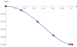
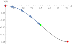
Figure 1: Incomplete RG: Schematic diagram of a UV to IR radial flow with a scalar operator with bulk potential $V(\phi)$. The complete RG flow in the flat boundary case (left) vs incomplete RG flow with a compact boundary (right). The flow in the later case terminates at the center of the space (the green point).

At the level of Einstein’s equations, one intuition we may develop from the study of holographic C-theorems for the flat case is that a relevant perturbation would dump negative energy inside the bulk. In the compact boundary case, the negative energy can’t escape and would be contained near the center of the bulk. This would lead to an anti-gravity effect and may have the following consequences:

Claims: 1

1

1. HP transition temperature may increase. Entropy difference at HP transition temperature may decrease.

   Thermal physics of a holographic theory defined with a compact boundary is more interesting than its non-compact counterpart. With a compact boundary we have a possibility of a Hawking-Page like de-confinement transition (HP)[5, 6]. This is a consequence of having a mass-gap in the boundary due to compactness. These kind of transition is often first order. In our case, dumping negative energy in the bulk makes formation of BH harder. Hence under a relevant deformation of the boundary theory, HP transition temperature may increase. Whereas the radius of the BH is expected to decrease at HP transition temperature. To note: entropy difference of two phases at the transition temperature is the area of the BH at that temperature.

2. A relevant deformation may dump more negative energy inside the space time leading to decrease in effective volume and increase in cosmological constant ($\Lambda$) of the bulk .

3. Mass scale of fundamental excitations of AdS is determined by $L$ or $\Lambda$ as $m^{2}\propto 1/L^{2}\propto\Lambda$. Hence any fundamental frequency associated with the AdS may increase if $\Lambda$ is increased.

4. Entanglement entropy If we look at entanglement (EE) of a boundary region with an area $A$, then $EE=c_{UV}A/a^{2}+\delta EE$, where $a$ is an UV cutoff. $c_{UV}$ is closely related to a central charge and at finite $J$, $\delta EE(J)<\delta EE(0)$. As we take bigger and bigger area, $\delta EE$ would increase in magnitude and then saturate for the largest area. As the space is compact the the area A may not be arbitrarily large. Largest value of $A_{max}$ is half big as the boundary area. For a boundary $S^{n}$, the largest area is given by the half-sphere.

5. We also expect: as we turn on a source J, $\delta EE$ would decrease monotonically with J. This behavior should be observed in easily calculable EE of $A_{max}$.

Figure 2: A schematic map of the paper showing the effects of turning on $J$. From left, reduction in the size of BH at HP transition. incerase in HP transtion temp, increase in $\delta_{EE}$, increase in the frequency of fundamental modes.

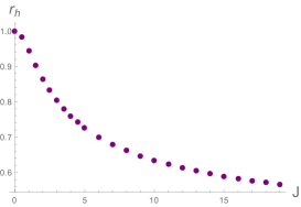
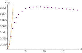
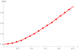
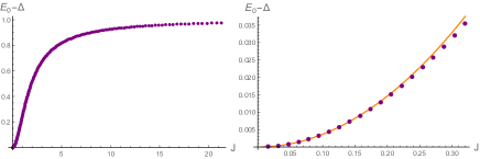
In practice we study the simplest setup to motivate our point. We consider a relevant scalar ($m^{2}=-2$) perturbation in global AdS4 background. The boundary of the spacetime is $S^{2}\times R$. The scalar field has the near-boundary asymptotic expansion

$$\phi=\frac{J(t)}{r}+\frac{\epsilon(t)}{r^{2}}+\ldots,$$ (1.3)

We turn on a time independent $J$ (and also $\epsilon$ in Section 5). In the Section 2 we construct the $T=0$ solution , which has been christened AdSJ. We prove a version of C-theorem and discuss the consequences in the Section 2.2. In the Section 3, we study the BH solution in AdSJ geometry and the Hawking-Page transition numerically. We also study a systematic perturbative computation of $T_{HP}$, in $J$ and match the perturbative result with our exact numerics. This has been done in the Section 4. We find broad similarity with Claims 1. In Appendix B.3, we discuss the approach to planar limit.

Scalar condensates, i.e. BH solutions with scalar hair have been discussed in works related to Holographic superconductors [9] as well as for global AdS [10, 11]. A scalar condensation induced by another scalar has been discussed in [12]. However, investigating any kind of second order phase transition [13] is not the focus of this work. The study of boson stars [14], a bosonic lump in space time, is more than half a century old and was pioneered by Wheeler and Kaup [15, 16]. Boson star like solutions are also constructed in AdS [17]. They are prevented from collapse by gravitation and/or by a boundary chemical potential corresponding to a global charge. Our solution is different and could be thought of as turning on a relevant operator in the boundary. As it is a relevant deformation, in some sense our AdSJ solution has a infinite negative mass.

2 Model & equations of motion and AdSJ solution

We consider four-dimensional Einstein gravity with a negative cosmological constant $\Lambda$ and a massive scalar field $\phi$. The action is

$$S=S_{EH}+S_{\phi}=\frac{1}{16\pi G}\int d^{d+1}x\sqrt{-g}(R-2\Lambda)-\int d^{d+1}x\sqrt{-g}\left[\frac{1}{2}(\partial\phi)^{2}+V(\phi)\right],$$ (2.1)

where the scalar field potential is given by $V(\phi)=\frac{1}{2}m^{2}\phi^{2}$, with $m^{2}=-2$. Unless stated otherwise in a explicit manner, we are working in units such that $4\pi G=1$ and $\Lambda=-3/L^{2}$, $L=1$. We are considering spherically symmetric solutions. Our metric ansatz is

$$ds^{2}=-Fe^{-2\delta}dt^{2}+F^{-1}dr^{2}+r^{2}d\Omega_{d-1}^{2},$$ (2.2)

where $\delta$, $F$ and the scalar field $\phi$ are functions of $t$ and $r$. The boundary of the AdS^d+1 lies at $r=\infty$ and the center is at $r=0$. We will confine ourselves to $d=3$. For our numerics we often use a co-ordinate redifination $\tan(x)=r$ (see Appendix A), which maps $r$ to a compact domain $x\in[0,\pi/2]$.

A useful field redefinition is given by

$$\Phi(t,r)=\phi^{\prime}(t,r)\ ,\qquad\Pi(t,r)=\frac{e^{\delta(t,r)}}{F(t,r)}\dot{\phi}(t,r)\,.$$ (2.3)

Upon this redefinition, the scalar field equations of motion can be cast in the form

$$\dot{\Phi} = \left(Fe^{-\delta}\Pi\right)^{\prime}\ ,$$ (2.4)

$$\dot{\Pi} = \displaystyle\frac{1}{r^{2}}\left(r^{2}Fe^{-\delta}\Phi\right)^{\prime}+2e^{-\delta}\phi\,.$$ (2.5)

From the Einstein equations we obtain

$$F^{\prime} = \displaystyle\frac{-F+3r^{2}+1}{r}-rF\left(\Pi^{2}+\Phi^{2}\right)+2r\phi^{2},$$ (2.6)

$$\delta^{\prime} = -\displaystyle r\left(\Phi^{2}+\Pi^{2}\right)\,.$$ (2.7)

For the static solutions relevant for the computation of the phase diagram, the equations reduce to

$$\delta^{\prime}(r)+r\phi^{\prime}(r)^{2}=0,$$

$$F^{\prime}(r)-F(r)\left(-r\phi^{\prime}(r)^{2}-\frac{1}{r}\right)-2r\phi(r)^{2}-3r-\frac{1}{r}=0,$$

$$\phi^{\prime\prime}(r)-\frac{\left(-F(r)-2r^{2}\phi(r)^{2}-3r^{2}-1\right)\phi^{\prime}(r)-2r\phi(r)}{rF(r)}=0.$$ (2.8)

The scalar field has the near-boundary asymptotic expansion

$$\phi=\frac{J(t)}{r}+\frac{\epsilon(t)}{r^{2}}+\ldots,$$ (2.9)

where $r$ is a radial Schwarzschild coordinate. In the standard quantization of the scalar field, $J$ corresponds to the source of the scalar operator $\mathcal{O}$ of conformal dimension $\Delta=2$ dual to $\phi$, while $\epsilon$ determines its vacuum expectation value; for the alternate quantization, the roles played by $J$ and $\epsilon$ get reversed.

The metric behaves as

$$F(r)=r^{2}+\left(J^{2}+1\right)-\frac{m_{0}}{r}+\frac{2\epsilon^{2}+2J^{4}+J^{2}}{r^{2}}+O\left(r^{-3}\right),$$ (2.10)

$$\delta(r)=\frac{J^{2}}{2r^{2}}+O\left(r^{-3}\right),$$ (2.11)

where we have chosen the gauge $\delta(\infty)=0$, which makes the coordinate $t$ to agree with the proper time of a static boundary observer. In our case, we are interested in determining how the introduction of a finite, time-independent and homogeneous source modifies the phase structure of black holes in asymptotic global AdS.

2.1 AdSJ solution

At the probe limit (small $J$), where the scalar amplitude is small and is gravitationally decoupled, we have (with $x=\tan^{-1}(r)$, see Appendix A),

$$\phi(x)=x\cot(x).$$ (2.12)

That gives $\epsilon/J=2/\pi$. The fully non-linear solutions for higher values of $J$ has been shown in Figure 3. We notice that the with increasing $J$ the scalar curvature ($R$) gets more negative and its amplitude increases inside the bulk.

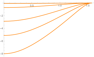
(a) Upper: Scalar field profile with $x$. Lower: $R$ vs $x$ plots. $J=0.3,0.7,1.1,1.7,2.5$, increasing away from the $x$-axis.

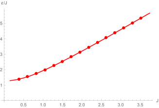
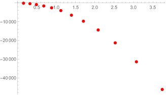
(b) Upper: $\epsilon/J$ vs $J$. Lower: Volume of the space vs $J$.

Figure 3: AdSJ solution and its properties.

2.2 C-theorems on a compact space

The holographic c-theorem(or it’s higher dimensional counterpart a-theorem) naturally appears in the context of a boundary deformation. In field theoretic context c-theorem implies that certain quantity (central charge) of a CFT increases monotonically under RG flow, whereas in holography it implies that there exists a monotonically varying function in the bulk, from the UV region to the IR. Holographic c-theorems are often discussed when the boundary is flat. However in our case the the boundary is $S^{3}\times S^{1}$, where the spatial part $S^{3}$ is a compact manifold with a finite volume. Compact manifold provides a natural IR cutoff to the RG flow, and RG flow may not continue to IR fixed point. We argue instead that c-theorem like arguments may be used to prove that a deformation in the boundary reduces the bulk volume. As we soon discuss, this has an interesting physical and geometrical consequence.

The proof of this theorem relies on the Null Energy condition, and uses the Einstein equations. Following in the footsteps of earlier calculations, we can quickly show that such a function exists in our case.
Consider the difference between $G_{t}^{t}$ and $G_{r}^{r}$, the Einstein tensors for the metric, which for this ansatz 2.2, equals to $\frac{2F(r)\delta^{\prime}(r)}{r}$. Using Einstein equations, this can be equated to

$$\frac{2F(r)\delta^{\prime}(r)}{r}=G_{t}^{t}-G_{r}^{r}=8\pi G(T_{t}^{t}-T_{r}^{r})$$ (2.13)

By the null energy condition, the right hand side is always non-positive. Hence, we can conclude that

$$\frac{2F(r)\delta^{\prime}(r)}{r}<0$$

Since the emblackening factor $F(r)$ is always positive in the region we’re interested in(outside the horizon for a Black-Hole and everywhere in the AdSJ case), it shows that

$$\delta^{\prime}(r)<0$$ (2.14)

We have now shown that a function exists whose radial derivative is always negative in the bulk.

This is, however, is not the only conclusion. If we look at the scalar field equation,

$$\partial_{r}(\sqrt{g}g^{rr}\partial_{r}\phi)=\sqrt{g}V^{\prime}(\phi)$$ (2.15)

the above equation leads to an attractor like mechanism [18]. For our case, the attractor mechanism says that $\phi^{2}$ is an monotonically decreasing function of the radial co-ordinate, i.e.

$$\phi\phi^{\prime}<0$$ (2.16)

. This monotonicity of $\phi^{2}$ follows from the fact that the scalar field $\phi$ and its double derivative with the radial coordinate (or any other monotonic reparametrization of $r$) has the same sign. Unlike attractor mechanism in flat space, $\phi$ reaches a finite value at the center of the space which implies $\phi^{\prime}(0)=0$ from smoothness.

Let’s look at the emblackening function $F(r)$. From (2), we get,

$$F^{\prime}(r)-F(r)\left(\delta^{\prime}-\frac{1}{r}\right)-2r\phi(r)^{2}-3r-\frac{1}{r}=0$$ (2.17)

$$\Rightarrow F(r)=\frac{1}{r}e^{\delta(r)}\int_{0}^{r}e^{-\delta(r)}(2r^{2}\phi^{2}+3r^{2}+1)dr$$ (2.18)

The above expression is a quantification of the intuitive claim that turning on $J$ augments the cosmological constant and dumps negative energy in the bulk. With a rearrangement of (2) we also have an alternative expression for the emblackening function:

$$F(r) =1+r^{2}+\frac{1}{r}\int_{0}^{r}-e^{\delta}\partial_{r}(r^{2}Fe^{-\delta}\phi\phi^{\prime})dr$$ (2.19)

$$=1+r^{2}-rF\phi\phi^{\prime}+\frac{1}{r}\int_{0}^{r}\delta^{\prime}r^{2}F\phi\phi^{\prime}dr$$ (2.20)

From (2.17) and (2.19) we may prove the following inequality,

$$1+r^{2}<F(r)<1+r^{2}+\frac{1}{r}\int_{0}^{r}2r^{2}\phi^{2}dr$$ (2.22)

giving us an idea how much $J$ affects the emblackening factor. In proving the above inequality we have used (2.16) and the monotonicity condition (2.16).

2.3 Volume of the space and EE

This helps us in making another important conclusion. The volume element, $e^{-\delta(r)}r^{2}\sin{\theta}$, from which we can write down the total (regularized and compared to global AdS4) volume of the spacetime to be

$$Vol=\int(e^{-\delta(r)}-1)r^{2}\sin{\theta}dtdrd\Omega$$

This volume decreases with the introduction of the scalar field as $e^{-\delta(r)}<1$.

Another quantity of interest is the EE. We would concentrate on calculating the Entanglement Entropy of a circular area in the boundary. Boundary is an $S^{2}\times R$ here. If we take an area ($A$) enclosed by a curve $\cal C$, then according to Ryu-Takyanagi [19] EE is the area of a maximal $d-2(=2)$ co-surface in AdSJ which ends on $\cal C$. For an area in boundary enclosed by a great circle ($A_{max}$), we have,

$$EE_{A_{max}} =2\pi\int_{0}^{r_{o}}\frac{r}{\sqrt{(}F(r))}\,dr$$ (2.23)

$F(r)=1+r^{2}$ for AdS4 and we have,

$$EE^{AdS4}_{A_{max}} \approx 2\pi(r-1)$$ (2.25)

The divergent first term is the ”area” contribution and the second term is ${\cal O}(1)$ negative contribution [20]. For AdSJ we have,

$$EE_{A_{max}} =2\pi\int_{0}^{r_{o}}\frac{r}{\sqrt{(}F(r))}\,dr=2\pi(r-\delta_{EE}(J))$$ (2.26)

From (2.22) we get,

$$EE^{AdSJ}_{A_{max}} <EE^{AdS4}_{A_{max}}$$ (2.28)

$$\Rightarrow\delta_{EE}(J) >1$$ (2.29)

. (2.30)

The ${\cal O}(1)$ contribution also seems to be increasing with $J$ from our numerics (see ).

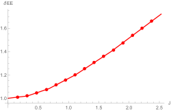
Figure 4: A plot of $\delta_{EE}$ vs $J$.

The extremal surface for EE calculation will venture more into the bulk as the size of the boundary region increases. Now because of the inequality (2.22), and the fact $F$ differs more from the $AdS4$ value of $f(r)=1+r^{2}$ as we go inside the bulk, we expect $\delta_{EE}$ to increase in magnitude with the size of the boundary region (see Claim 1).

2.4 Normal modes of the AdSJ solution

The purpose of this section is to discuss the computation of normal modes of the AdSJ solution. We decompose the scalar field and metric as (using co-ordintes defined in Appendix A),

$$\phi(t,x)=\phi_{s}(x)+\gamma\cos{\omega t}\,\phi_{1}(x),$$ (2.31)

$$f(t,x)=f_{s}(x)+\gamma\cos{\omega t}\,f_{1}(x),$$ (2.32)

$$\delta(t,x)=\delta_{s}(x)+\gamma\cos{\omega t}\,\delta_{1}(x).$$ (2.33)

where the subscript s refers to the background AdSJ solution, and $\omega$ is the frequency of the normal mode. By expanding the equations of motion to first order in the mode amplitude $\gamma$, we get the equations of motion for these fluctuations. The reason for choosing this particular ansatz is that the overall time dependence in these equations factorizes.

It is important to realize that the momentum constraint equation becomes, at first order, an algebraic relation that is solved by

$$f_{1}(x)=-2\cos x\sin x\,\phi_{s}^{\prime}(x)\phi(x).$$ (2.34)

In the same way, from the equation of motion for $\delta$ we get that

$$\delta_{1}^{\prime}(x)=-2\cos x\sin x\,\phi_{s}^{\prime}(x)\phi_{1}^{\prime}(x).$$ (2.35)

Therefore, the only independent dof of the problem is $\phi_{1}(x)$. Its equation of motion follows from the scalar field’s, once we take into account the relations between $f_{1}$, $\delta_{1}$ and $\phi_{1}$. The final result is a complicated but a linearized eigenvalue equation for $\phi_{1}(x)$,

$$\phi_{1}^{\prime\prime}(x)+F_{1}(x)\phi_{1}^{\prime}(x)+(\omega^{2}F_{3}(x)+F_{2}(x))\phi_{1}(x)=0.$$ (2.36)

$$F_{1}(x)=\frac{-\cot x+2\csc x\sec x+\tan x+\cos 2x\csc x\sec xf_{s}(x)+2\tan x\,\phi_{s}(x)^{2}}{f_{s}(x)}$$

$$F_{2}(x)=\frac{2\left(\sec^{2}x+4\tan x\,\phi_{s}(x)\phi_{s}^{\prime}(x)-(\cos 2x-2)\phi_{s}^{\prime}(x)^{2}+2\sin^{2}x\,\phi_{s}(x)^{2}\phi_{s}^{\prime}(x)^{2}\right)}{f_{s}(x)}$$

$$F_{3}(x)=\frac{e^{2\delta_{s}(x)}}{f_{s}(x)^{2}}$$

The value of frequency $\omega$ is determined by imposing the following boundary conditions:

• Smoothness at the origin, i.e., $\phi_{1}^{\prime}(0)=0$.

• Normalizability. The source $J$ that supports the AdSJ is kept invariant by the perturbation, i.e., $\phi_{1}^{\prime}(\pi/2)=0$.

The numerical values of the lowest eigenfrequency are plotted in Fig.5a. We observe that at large $J$, the eigenfrequency saturates to a constant value. On the other hand, at small $J$ it reduces to its value on the AdS₄ background, plus a positive quadratic correction.

The value of this quadratic correction can be computed perturbatively, by expanding $\phi_{1}(x)=\phi_{1,0}(x)+J^{2}\phi_{1,2}(x)$, $\omega=2+\omega_{2}J^{2}$ and introducing these expressions with (4.9)-(4.11) and (4.15)-(4.17) into (2.36), expanding them to order $J^{2}$. First, we find that $\phi_{1,0}$ is given by the lowest normal mode of the scalar field on the AdS₄ bakground,

$$\phi_{1,0}(x)=\cos^{2}x,$$ (2.37)

as expected. The crucial point is that, at the next order, the requirement that $\phi_{1,2}$ is simultaneously normalizable and regular can only be met if the second order correction to the frequency, $\omega_{2}$, takes the value

$$\omega_{2}=3-\frac{26}{\pi^{2}}=0.365649>0.$$ (2.38)

In Fig.5b, we plot the numerical results for the lowest eigenfrequency (purple dots) vs this perturbative prediction (solid orange). It is clear that at small $J$ both computations agree very well.

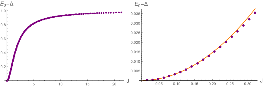
Figure 5: Left: Difference between the lowest eigenfrequency of the AdSJ, $E_{0}$, and its value on the AdS₄ vacuum, $\omega_{0}=\Delta=2$, as a function of the source $J$ supporting the AdSJ background. Right: as in the left plot, but for smaller $J$. The solid orange line is the leading order dependence of $E_{0}$ on $J$ predicted by perturbation theory.

It is natural to interpret the value of $E_{0}$ as the mass gap of the dual field theory, in the sense that $E_{0}$ sets the rest energy of the lighest scalar excitation. Heuristically, we might assume that, since the typical size of this excitation should scale as $1/E_{0}$, the deconfinement temperature must also be proportional to $E_{0}$, as we would need a medium of thermal wavelength $\epsilon\sim 1/E_{0}$ to resolve the size of the scalar glueball and melt it. If this expectation is correct, the fact that $E_{0}$ tends to a constant in the large $J$ limit leads to the prediction that the Hawking-Page temperature should also saturate in this limit.^,

2.4.1 Massless scalar field modes on the AdSJ background

The purpose of this section is to compute the normal modes of a probe massless scalar field $\psi$ on the AdSJ background. The underlying idea is interpreting these normal modes as a proxy for the mesonic excitations in the system. Note that $\psi$ is different from the scalar field $\phi$ that sources the geometry. Given that $\psi$ is a probe field, its equation of motion on the AdSJ background is given by

$$\partial_{a}\left(\sqrt{-g_{s}}g_{s}^{ab}\partial_{b}\psi\right)=0,$$ (2.39)

where $g_{s}$ is the AdSJ metric. If we assume that $\psi$ is spherically symmetric and decompose $\psi(t,x)=\hat{\psi}(x)e^{-i\omega t}$, we get (using the co-ordintes defined in Appendix A)

$$\hat{\psi}^{\prime\prime}(x)+\left(2\csc x\sec x+\frac{f_{s}^{\prime}(x)}{f_{s}(x)}-\delta_{s}^{\prime}(x)\right)\hat{\psi}^{\prime}(x)+\frac{e^{2\delta_{s}(x)}\omega^{2}}{f_{s}(x)^{2}}\hat{\psi}(x)=0,$$ (2.40)

where the subscript $s$ refers to quantities evaluated on the AdSJ background. Equation (2.40) is to be solved demanding that $\hat{\psi}(x)$ is regular at $x=0$, $\lim_{x\to 0}x\hat{\psi}(x)=0$, and normalizable, $\hat{\psi}(x=\pi/2)=0$. Provided that these boundary conditions are imposed, $\omega$ corresponds to a normal mode frequency.

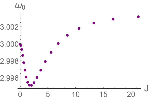
Figure 6: Fundamental mode of a probe massless scalar field on the AdSJ background.

We have solved (2.40) numerically, employing a pseudospectral algorithm. Since neither (2.40) nor the boundary conditions we are imposing distinguish between the standard and the alternative quantization for $\psi$, we only need to solve the problem once for each AdSJ solution. In Fig. 6 we plot the frequency of the lowest normal mode, $\omega_{0}$, against $J$ (the plot in terms of $\epsilon$ is qualitatively similar). It is manifest that the behavior of the lowest eigenfrequency is not correlated at all with the behavior of the Hawking-Page temperature, neither in the standard nor in the alternative quantization.

3 Deconfinement and BHs at finite J

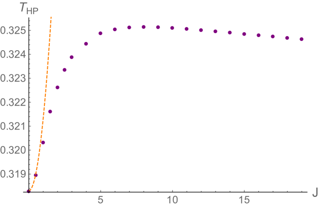
Figure 7: Phase transition temperature $T_{HP}$ vs relevant coupling $J$ (purple dots). The leading order perturbative prediction for $T_{HP}$ (eqn. (4.34)) corresponds to the dashed orange line.

In this section we undertake the task of determining the grand-canonical phase diagram of our theory at finite $J$ and $T$. At $J=0$, the well known story of Hawking-Page transition [6, 5] is the following. At $T=0$ there exists only one semi-classical solution which is global AdS. As the temperature is increased, at the nucleation point $T=T_{N}$, a new solution of big and small black holes become possible classical saddles. At the nucleation point both big and small black holes have the same mass and size. As temperature is increased further, the area(also the entropy) of the big black hole increases and the the opposite happens for small black holes. At $T=T_{HP}$ the free energy of the big BH becomes more than global AdS and the it becomes the dominating saddle. This is identified with deconfinement transition in the boundary theory [5]. Possibly, there exist a few other gravity solutions including BH solutions, and even at a higher temperature transitions like hegadorn transition are possible [21]. We won’t expound upon these directions in this work.

3.1 The free energy computation at finite $J$

In order to find out which solution dominates the grandcanonical partition function at a given point in the $(J,T)$-plane, we need to calculate their Gibbs free energy.

As usual, the free energy $F$ is given by the renormalized Euclidean on-shell action of the solution as $F=TS_{E}$. To compute this quantity, we have to add a series of countertems to the action (2.1) in such a way that, for our choice of boundary conditions, $S_{E}$ is stationary on the saddle points we are interested in. This is equivalent to the statement that the variational problem is well-defined; as a byproduct, the resulting action comes out finite.

The full computation of $S_{E}$ can be found in appendix B. We quote below the final result for the free energy density

$$f\equiv\frac{F}{\textrm{Vol}(S^{2})}=-\frac{m_{0}}{16\pi G}-J\epsilon+\frac{r_{IR}}{8\pi G}+\int_{r_{IR}}^{\infty}dr\frac{1-e^{-\delta(r)}}{8\pi G},$$ (3.1)

where $r_{IR}=0,r_{h}$ for AdSJ and black holes respectively.

3.2 Results

The fundamental qualitative story of the HP transition remains almost the same at finite $J$. At $T=0$ there exists only one classical solution which is global AdSJ with no horizon but a nontrivial scalar field profile. At higher temperatures, there is another competing semiclassical saddle: the big hairy BH, which becomes dominant at a coupling dependent transition temperature $T_{HP}(J)$. However, the coupling $J$ has a significant influence on the entropy difference at the phase transition: as $J$ increases, this entropy difference goes down. In order to illustrate this, in Fig. 8 we plot how the radius of the first thermodynamically dominant black hole changes with the coupling. Its decrease is manifest. This monotonic decrease is enough to overcome the small variations of $T_{HP}$. In Fig. 7, we plot the Hawking-Page temperature as a function of the relevant coupling $J$. We note that $T_{HP}$ is monotonic for small enough $J$ and we have demonstrated that with a perturbative analysis. We also see that $T_{HP}(J)>T_{HP}(0)$ for all $J$. As discussed in Appendix B.3, this last behavior is compatible with the absence of a planar limit for the Hawking-Page transition. Unfortunately, we have been unable to determine beyond any trace of doubt whether $T_{HP}$ approaches zero as $J\to\infty$ or saturates to a finite value.

It is manifest that $T_{HP}$ is not globally monotonic: there is a maximum temperature $T_{HP}^{*}=0.3252$, which is attained at $J^{*}=8.124$. Past this point, $T_{HP}$ decreases. It must be noted that, overall, the relevant coupling has a small influence on the value of $T_{HP}$. Our numerical results strongly suggest that $T_{HP}$ never exceeds $T_{HP}^{*}$ and as we discussed $T_{HP}$ never goes below it’s zero temperature value $1/\pi$ for large $J$. If this is the case, the maximum relative variation of $T_{HP}$ with the coupling would be given by $(T_{HP}^{*}-1/\pi)/(1/\pi)=2.155\,\%$.

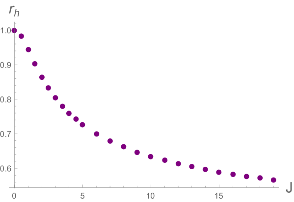
Figure 8: Radius of the first thermodynamically dominant black hole in terms of the coupling.

Solution at large J

This subsection sums up the numerical results we have found for $T_{HP}(J)$ at arbitrary coupling. To obtain reliable results, we are forced to be extremely precise in determining the free energy densities of the AdSJ and black hole solutions. To this end, we have solved equations (A) employing a pseudospectral method, checking our results by monitoring the agreement between expressions (3.1) and (4.36).

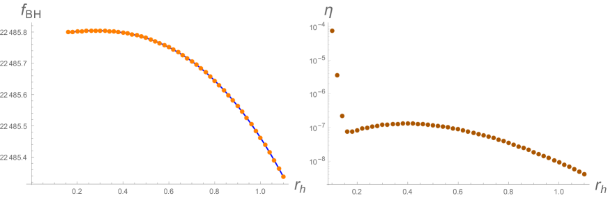
Figure 9: Left: At $J=45$, free energy density of the black hole family as computed by eqn. (3.1) (orange dots) and by the Smarr relation (4.36) (solid blue). Right: The agreement of the results of the left plot, as measured by the relative error parameter $\eta$.

As an example of the power of the pseudospectral method we have employed, in Fig. 9 we consider the black hole family with $J=45$ and compare expressions (3.1) and (4.36) for the free energy density. The grid we have employed for this computation consists of $121$ collocation points. We have introduced the quality parameter $\eta$, defined as

$$\eta=\frac{|f_{1}-f_{2}|}{(f_{1}+f_{2})/2}100,$$ (3.2)

where sub-indices $1$,$2$ refer to the free energy densities computed with each method. As we can see, they are in excellent agreement: at this coupling, the phase transition takes place at $r_{h}=0.49682$; according to Fig. 9, the relative error in the black hole free energy density at that radius is $O(10^{-7}\,\%)$.

4 The perturbative computation of $T_{HP}(J)$

It is desirable to check our numerical results against a (semi)analytic computation. To this end, we are going to show how the lowest order correction to $T_{HP}$ can be determined with almost no effort. Here we focus on $J<<1$ limit. We are going to compute this correction in two alternative ways. The first one requires only the knowledge of the expression for the free energy derived in the previous section. The second one relies essentially on the First Law (it is essentially the derivation of the Clausius-Clapeyron relation for our problem).

4.1 First method

The argument we employ is the following. We know that, at $J=0$, the radius of the first thermodynamically dominant black hole is $r_{c}^{0}=1$, where

$$f_{BH}^{0}(r_{c}^{0})=0.$$ (4.1)

At finite $J$, this Schwarzschild black hole is replaced by a hairy black hole with the same horizon radius, while global AdS₄ is replaced by a AdSJ background. Therefore, the difference in their free energies gets modified as

$$\Delta f=f_{BH}(r_{c}^{0})-f_{s}\neq 0,$$ (4.2)

and the phase transition does not happen at $r_{c}=r_{c}^{0}$ anymore. At leading order,

$$f_{BH}(r_{h})=f_{BH}^{0}(r_{h})+J^{2}\delta f_{BH}(r_{h}),$$ (4.3)

$$f_{s}=J^{2}\delta f_{s},$$ (4.4)

and so the free energy difference is

$$\Delta f=f_{BH}^{0}(r_{h})+J^{2}(\delta f_{BH}(r_{h})-\delta f_{s})+O(J^{4})$$ (4.5)

The crucial observation is that, also at $O(J^{2})$, we expect that the horizon radius at which the phase transition takes place changes as

$$r_{c}=r_{c}^{0}+J^{2}\delta r_{c}=1+J^{2}\delta r_{c}.$$ (4.6)

Substituting this expression into the free energy difference, we see that, at leading order, it is sufficient to evaluate the change in the black hole free energy at $r_{c}^{0}$, since corrections coming from the change in $r_{c}$ only change this term at order $J^{4}$. Therefore, at the phase transition point, we have that

$$\begin{split}\Delta f=&f_{BH}^{0}(r_{c}^{0}+J^{2}\delta r_{c})+J^{2}(\delta f_{BH}(r_{c}^{0})-\delta f_{s})=f_{BH}^{0}(r_{c}^{0})+J^{2}\left(\frac{df_{BH}^{0}}{dr}(r_{c}^{0})\delta r_{c}+\delta f_{BH}(r_{c}^{0})-\delta f_{s}\right)\\ =&J^{2}\left(\frac{df_{BH}^{0}}{dr}(r_{c}^{0})\delta r_{c}+\delta f_{BH}(r_{c}^{0})-\delta f_{s}\right)=0,\end{split}$$ (4.7)

up to terms $O(J^{4})$. To determine the radius of the first thermodynamically dominant black hole at finite but small coupling, we just need:

• $f_{BH}^{0}$ as a function of $r_{h}$.

• $\delta f_{BH}(r_{c}^{0})$, which involves solving for the scalar field and metric fluctuations over the Schwarzschild black hole of horizon radius $r_{c}^{0}=1$.

• $\delta f_{s}$.

The first and third quantities of the list above can be determined analytically; the second requieres a straightforward numerical computation, since the linearized Klein-Gordon equation for the scalar field in the Schwarzschild black hole background is not exactly solvable (in global coordinates).

The first quantity is easily shown to be equal to

$$\frac{df_{BH}^{0}}{dr}(r_{c}^{0})=\frac{1-3r^{2}}{16\pi G}\bigg{\rvert}_{r_{h}=r_{c}^{0}=1}=-\frac{1}{8\pi G}=-\frac{1}{2}$$ (4.8)

in our units. On the other hand, in order to determine the AdSJ free energy, we need to find the AdSJ solution at $O(J^{2})$. This is achieved by solving the linearized Klein-Gordon and Einstein equations over global AdS₄. We seek a time-independent, spherically symmetric solution supported by a nontrivial scalar field profile. Expanding in $J$

$$\phi(r)=J\phi_{1}(r),$$ (4.9)

$$f(r)=(1+r^{2})+J^{2}f_{2}(r),$$ (4.10)

$$\delta(r)=J^{2}\delta_{2}(r),$$ (4.11)

we obtain the following equations of motion for the fluctuations

$$\left(4r^{2}+2\right)\phi_{1}^{\prime}(r)+r\left(r^{2}+1\right)\phi_{1}^{\prime\prime}(r)+2r\phi_{1}(r)=0,$$ (4.12)

$$r\left(f_{2}^{\prime}(r)+r\left(r^{2}+1\right)\phi_{1}^{\prime}(r){}^{2}-2r\phi_{1}(r){}^{2}\right)+f_{2}(r)=0,$$ (4.13)

$$\delta_{2}^{\prime}(r)+r\phi_{1}^{\prime}(r){}^{2}=0,$$ (4.14)

which are solved by

$$\phi_{1}(r)=\frac{2\tan^{-1}(r)}{\pi r},$$ (4.15)

$$f_{2}(r)=\frac{4\tan^{-1}(r)\left(\left(r+\frac{1}{r}\right)\tan^{-1}(r)-1\right)}{\pi^{2}r},$$ (4.16)

$$\delta_{2}(r)=\frac{1}{2}-\frac{2\left(\frac{1}{r^{2}+1}+\left(1-\frac{1}{r^{2}}\right)\tan^{-1}(r)^{2}+\frac{2\tan^{-1}(r)}{r}\right)}{\pi^{2}}.$$ (4.17)

The boundary conditions are as follows:

• We have demanded that $\phi_{1}$ is regular at the origin, and also that $r\phi_{1}(r)\rightarrow 1$ as $r\rightarrow\infty$ -this is needed in order to set $J$ as the actual source.

• We demand that $f_{2}$ is regular at the origin.

• We set $\delta_{2}(\infty)=0$ to work in the boundary time gauge.

Once the solution is known, we can employ it to compute $\delta f_{s}$. For AdSJ, we have

$$f_{s}=-\frac{m_{0}}{16\pi G}-J\epsilon-\frac{1}{8\pi G}\int_{0}^{\infty}dr\left(e^{-\delta(r)}-1\right).$$ (4.18)

From our solution, at leading order

$$m_{0}=(6/\pi)J^{2},$$ (4.19)

$$\epsilon=-(2/\pi)J,$$ (4.20)

$$\int_{0}^{\infty}dr\left(e^{-\delta(r)}-1\right)=-(1/\pi)J^{2}.$$ (4.21)

In our units ($4\pi G=1$), we have

$$f_{s}=\delta f_{s}J^{2}=\frac{1}{\pi}J^{2}$$ (4.22)

or $\delta f_{s}=1/\pi$.

The final step is finding the first correction in $J$ to the Schwarzschild black hole of $r_{h}=1$. Again, we linearize our fields as

$$\phi(r)=J\phi_{1}(r),$$ (4.23)

$$f(r)=f_{0}(r)+J^{2}f_{2}(r),$$ (4.24)

$$\delta(r)=J^{2}\delta_{2}(r),$$ (4.25)

where $f_{0}(r)=-\frac{m_{0}}{r}+r^{2}+1$. For the black hole we are interested in, $m_{0}=2$. The scalar field equation reduces to

$$\frac{2\left(\left(2r^{3}+r-1\right)\phi_{1}^{\prime}(r)+r^{2}\phi_{1}(r)\right)}{r\left(r^{3}+r-2\right)}+\phi_{1}^{\prime\prime}(r)=0,$$ (4.26)

and, as for the AdSJ case, $f_{2},\delta_{2}$ can be determined by a simple integration once $\phi_{1}$ is known. Unfortunately, we have been unable to solve this equation analytically. We have proceeded by integrating it numerically. The equation is linear; we fix the freedom in rescaling $\phi_{1}$ by demanding that $r\phi_{1}(r)\rightarrow 1$ as $r\rightarrow\infty$, which corresponds again to setting $J$ as the actual field theory source. In this case, the free energy is given by

$$f_{BH}(1)=-\frac{m_{0}}{16\pi G}-J\epsilon+\frac{1}{8\pi G}-\frac{1}{8\pi G}\int_{1}^{\infty}dr\left(e^{-\delta(r)}-1\right).$$ (4.27)

At $O(J^{2})$,

$$f_{BH}(1)=\delta f_{BH}(1)J^{2}=-\frac{\delta m_{0}J^{2}}{16\pi G}-\delta\epsilon J^{2}-\frac{1}{8\pi G}\int_{1}^{\infty}dr\left(-\delta_{2}(r)J^{2}\right).$$ (4.28)

We have

$$\delta m_{0}=\frac{r^{4}}{6}f_{2}^{(3)}\left(r\right)|_{\infty}=1.967,$$ (4.29)

$$\delta\epsilon=-0.6555,$$ (4.30)

$$\int_{1}^{\infty}dr\delta_{2}(r)=0.2349.$$ (4.31)

Therefore,

$$\delta f_{BH}(\infty)=0.2813.$$ (4.32)

From eq. (4.7), we find that the phase transition takes place at a horizon radius such that

$$\delta r_{c}=-0.9296.$$ (4.33)

Therefore, the radius of the first thermodynamically dominant black hole decreases with respect to its position at $J=0$. Finally, the temperature of this black hole, i.e., the Hawking-Page transition temperature, changes as

$$T_{HP}(J)=T_{HP}(0)+J^{2}\delta T_{HP}=\frac{1}{\pi}+J^{2}\frac{2\delta r_{c}-4\delta_{2}(1)+f_{2}^{\prime}(1)}{4\pi}=\frac{1}{\pi}+0.003011344J^{2}.$$ (4.34)

The Hawking-Page temperature increases with increasing coupling. To obtain the expression above, we have expanded the formula for the black hole temperature to $O(J^{2})$,

$$T_{BH}=\frac{1}{4\pi}f^{\prime}(r_{h})e^{-\delta(r_{h})}=\frac{\frac{1}{r_{h}}+3r_{h}}{4\pi}+\frac{f_{2}^{\prime}(r_{h})-\delta_{2}(r_{h})(\frac{1}{r_{h}}+3r_{h})}{4\pi}J^{2}$$ (4.35)

and evaluated it at the phase transition point, $r_{h}=1+\delta r_{c}J^{2}$, keeping only terms up to $O(J^{2})$.

Numerical results are compared to this perturbative formula in Fig. 10.

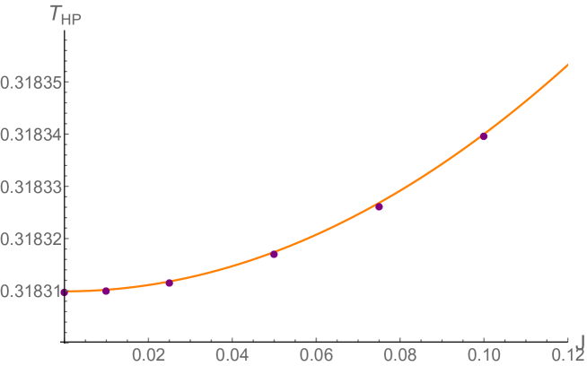
Figure 10: Perturbative prediction for $T_{HP}$ -solid orange- and actual values coming from a full fledged numerical computation -purple dots-. The agreement is extremely good.

4.2 Second method

Let me introduce, without writing the explicit proof, the following identities

$$f=\frac{1}{2}m_{0}+J\epsilon-Ts,$$ (4.36)

$$Tds=\frac{1}{2}dm_{0}+Jd\epsilon+2\epsilon dJ.$$ (4.37)

Taking a variation of (4.36), and with the help of (4.37),

$$df=\frac{1}{2}dm_{0}+Jd\epsilon+\epsilon dJ-Tds-sdT=-sdT-\epsilon dJ.$$ (4.38)

Upon an infinitesimal change in $J$, $J\rightarrow J+dJ$, the phase transition point changes as

$$f_{s}+df_{s}=f_{BH}+df_{BH}.$$ (4.39)

Taking into account that at the phase transition point $f_{s}=f_{BH}$, we obtain

$$0=df_{s}-df_{BH}=\left(-\epsilon_{s}+s_{BH}\frac{dT_{HP}}{dJ}+\epsilon_{BH}\right)dJ.$$ (4.40)

The above relation allows us to determine $T_{HP}^{\prime}(J)$,

$$T_{HP}^{\prime}(J)=\frac{1}{s_{BH}}\left(\epsilon_{s}-\epsilon_{BH}\right).$$ (4.41)

The quantities $s_{BH},\epsilon_{BH}$ and $\epsilon_{s}$ are evaluated at the Hawking-Page temperature at coupling $J$.

We know that, at first nontrivial order in $J$, $\epsilon_{s}=-2/\pi J$ and $\epsilon_{BH}=-0.6555...J$. The Hawking-Page transition in the absence of a source happens at $x_{c}^{0}=\pi/4$, and therefore $s_{BH}=1/(4G)=\pi$ in our units. Then,

$$T_{HP}^{\prime}(J)=\frac{1}{\pi}\left(-2/\pi+0.6555...\right)J.$$ (4.42)

Integrating (with the boundary condition that $T_{HP}(0)=1/\pi$),

$$T_{HP}(J)=\frac{1}{\pi}+0.00301128J^{2}+O(J^{4}).$$ (4.43)

We clearly see that the corrections determined by both methods agree very well; the relative difference between (4.34) and (4.43) is $<0.01\%$, and most likely due to accumulated numerical error.

5 Same story Different quantization: Alternative quantization

In the alternative quantization, the physical roles played by $J$ and $\epsilon$ are interchanged: now $\epsilon$ corresponds to the source of a $\Delta=1$ scalar operator, while $J$ corresponds to its vacuum expectation value. Therefore, in this section we are interested in the dependence of the Hawking-Page temperature with $\epsilon$.

5.1 Perturbative computation of the Hawking-Page temperature

Once expressions (B.36) and (LABEL:smarr_alt) are known, we can compute $T_{HP}$ in the alternative quantization along the lines of subsection 4.1 or 4.2. For concreteness, we will employ the Clausius-Clapeyron version of the derivation.

From (LABEL:smarr_alt), we have that

$$df=\frac{1}{2}dm_{0}+2Jd\epsilon+2\epsilon dJ-Tds-sdT.$$ (5.1)

Using the First Law (4.37) in the expression above, we get

$$df=-sdT+Jd\epsilon.$$ (5.2)

Moving along the phase transition curve, we have again that $f_{s}+\frac{df_{s}}{d\epsilon}d\epsilon=f_{BH}+\frac{df_{BH}}{d\epsilon}d\epsilon$. Since $f_{s}=f_{BH}$ along the curve, (5.2) implies that

$$\frac{dT_{HP}}{d\epsilon}=\frac{1}{s_{BH}}(J_{BH}-J_{s}),$$ (5.3)

which is equivalent to (4.41) with the substitutions $J\to\epsilon$, $\epsilon\to-J$.

Again, equation (5.3) is an exact statement, valid at any source $\epsilon$. To employ it to compute the first perturbative correction to $T_{HP}$, we must determine how $J$ depends on $\epsilon$ for $\epsilon\ll 1$, both for the AdSJ solution and the hairy black hole of horizon radius $x_{h}=\pi/4$.

A strategy analogous to the one employed in subsection 4.1 tells us that

$$J_{s}=-\frac{\pi}{2}\epsilon+O(\epsilon^{2}),\leavevmode\nobreak\ \leavevmode\nobreak\ \leavevmode\nobreak\ \leavevmode\nobreak\ \leavevmode\nobreak\ \leavevmode\nobreak\ J_{BH}=-1.5255\epsilon+O(\epsilon^{2}).$$ (5.4)

Recaling that at $\epsilon=0$, $s_{BH}=1/(4G)=\pi$

$$T_{HP}^{\prime}(\epsilon)=\frac{1}{\pi}(-1.5255+\pi/2)\epsilon=0.0144319\epsilon.$$ (5.5)

Taking into account that $T_{HP}(\epsilon=0)=1/\pi$, we finally have that

$$T_{HP}(\epsilon)=\frac{1}{\pi}+0.00721596\epsilon^{2}+O(\epsilon^{4}).$$ (5.6)

As for the standard quantization of the scalar field, the perturbative prediction is that the Hawking-Page temperature increases with the relevant coupling. In Fig. 11 we contrast this expectation against exact numerical results in the small coupling regime, finding excellent agreement.

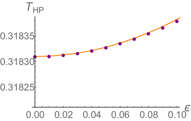
Figure 11: Perturbative prediction for $T_{HP}$ -solid orange- and actual values coming from a full fledged numerical computation -purple dots-. The agreement is extremely good.

5.2 Fully nonlinear results

In this case, and in contrast to what happened in the standard quantization, our numerical results show that the Hawking-Page temperature is monotonic, saturating to a finite value as $\epsilon\to\infty$ (see Fig. 12). Again, this is compatible with the absence of a planar limit for the Hawking-Page transition.

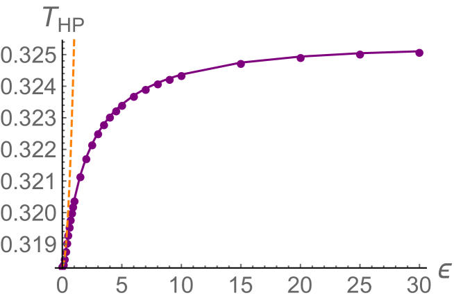
Figure 12: Phase transition temperature $T_{HP}$ vs relevant coupling $\epsilon$ (purple dots). The leading order perturbative prediction for $T_{HP}$ (eqn. (4.34)) corresponds to the dashed orange line.

As in the standard quantization case, the Hawking-Page temperature is mildly affected by the increasing relevant coupling (for instance, for the last coupling we have considered, $\epsilon=\epsilon_{max}=65$, we have that $(T_{HP}(\epsilon_{max})-T_{HP}(0))/T_{HP}(0)\approx 2.15\%$). As before, the entropy released at the phase transition also shows a marked decrease (see Fig. 13).

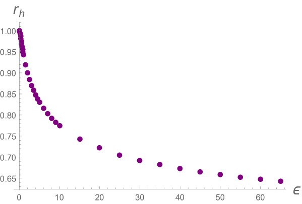
Figure 13: Radius of the first thermodynamically dominant black hole in terms of the coupling.

5.3 Normal modes of the AdS$\epsilon$ solution

In order to determine the normal modes of the AdS$\epsilon$ solution, we need to solve equation (2.36) with the following boundary conditions for $\phi_{1}$

• Origin regularity, i.e., $\phi_{1}(0)<\infty$.

• Normalizability. The source $\epsilon$ that supports the AdSJ is kept invariant by the perturbation, i.e., $\phi_{1}^{\prime\prime}(\pi/2)=0$.

Using the same pseudospectral code as before, we get the results displayed in Fig. 14a. Unlike in the standard quantization case, here the behavior of the lowest eigenfrequency of the AdSJ is correlated with the behavior of the Hawking-Page temperature.

The first correction to the lowest eigenfrequency can be computed again in an expansion in $\epsilon$. The result is

$$\omega_{0}=1+\left(\frac{3\pi^{2}}{8}-1\right)\epsilon^{2}+O(\epsilon^{4})$$ (5.7)

and is compared to the exact numerical values in Fig. 14b, finding very good agreement.

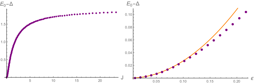
Figure 14: Left: Difference between the lowest eigenfrequency of the AdSJ, $E_{0}$, and its value on the AdS₄ vacuum, $\omega_{0}=\Delta=1$, as a function of the source $\epsilon$ supporting the AdSJ background. Right: as in the left plot, but for smaller $\epsilon$. The solid orange line is the leading order dependence of $E_{0}$ on $\epsilon$ predicted by perturbation theory.

6 Conclusion

In this work we discussed the how a compact boundary cuts down the holographic RG flow leading to an incomplete RG flow. We further discussed the implication of the incomplete RG flow for various physically relevant issues including black hole formation and deconfinement transition. We believe our results to be true in other dimensions and relevant scalar operators with different dimensions. It would be interesting to investigate physics of double trace deformations [22] in finite temperature and with a compact boundary. Another natural extension of our work may be in the case of the magnetic branes [23] and holographic lattices [24]. Instead of a theory with compact boundary, if we consider a confining theory, like say AdS solition with boundary $S^{2}\times S^{1}\times S^{1}$, then also we hope to phenomena similar to incomplete RG flow [25]. We noted how turning on a relevant scalar operator in the boundary introduces negative energy in the bulk; virtually increasing the effective cosmological constant. We may speculate whether this negative energy may be used to sustain an worm hole [26] and whether there are alternative ways to sustain a traversable wormhole [27].

7 Acknowledgment

We thank Alexandre Serantes Rubianes for discussions and collaboration at various stages of this project. PB thanks Jyotirmoy Bhattacharya, Vishnu Jejjala for discussions. PB also thanks Robert De Mello Koch and other organizers of MITP including workshop in Durban 2020, where this work was presented.

Appendix A An alternative co-ordinate system

Another alternative co-ordinate system to use $(t,r,\theta,\phi)\rightarrow(t,x,\theta,\phi)$ with $\tan(x)=r$. This co-oridante has the advantage of a finite domain $x\in[0,\frac{\pi}{2}]$. In our numerical analysis we often use this coordinate because a finite domain often facilitates the numerics and makes plots more revealing. We use following spherically symmetric metric ansatz:

$$ds^{2}=\sec^{2}x(-fe^{-2\delta}dt^{2}+f^{-1}dx^{2}+\sin^{2}xd\Omega_{d-1}^{2}),$$ (A.1)

where $\delta$, $f$ and the scalar field $\phi$ are functions of $t$ and $x$. $d\Omega_{d-1}^{2}$ is the metric on $d-1$ sphere. If $f=1,\delta=0$, the above ansatz becomes a global AdS^d+1 space. We note that definition of the blackening factor in (A.1) is slightly different than (2.2).

For the static and symmetric solutions relevant for the computation of the phase diagram, the equations reduce to

$$\delta^{\prime}(x)+\sin(x)\cos(x)\phi^{\prime}(x)^{2}=0,$$

$$f^{\prime}(x)+f(x)\sin(x)\cos(x)\phi^{\prime}(x)^{2}+(f(x)-1)\tan(x)\left(\csc^{2}(x)+2\right)-2\phi(x)^{2}\tan(x)=0,$$

$$\phi^{\prime\prime}(x)+\left(\frac{f^{\prime}(x)}{f(x)}-\delta^{\prime}(x)+2\csc(x)\sec(x)\right)\phi^{\prime}(x)+\frac{2\sec^{2}(x)}{f(x)}\phi(x)=0.$$ (A.2)

Appendix B Holographic renormalization

B.1 Holographic renormalization: standard quantization

Let us consider first the variation of the scalar field action. After integrating by parts and employing the equations of motion, we are left with

$$\delta S_{\phi}=-\int_{r=R}dtd\theta d\varphi\sqrt{-h}n^{r}\partial_{r}\phi\delta\phi,$$ (B.1)

where $n^{\mu}$ is the outward unit normal to a constant $r=R$ hypersurface,

$$n^{\mu}=(0,\sqrt{F(r)},0,0)$$ (B.2)

and $\sqrt{-h}=r^{2}e^{-\delta(r)}\sqrt{F(r)}\sin\theta$ is the determinant of the induced metric on this hypersurface,

$$dh^{2}=-F(r)e^{-2\delta(r)}dt^{2}+r^{2}d\Omega^{2}.$$ (B.3)

For scalar field fluctuations $\delta\phi$ such that $\delta J=0$,

$$\delta\phi=\frac{\delta\epsilon}{r^{2}}+\ldots,$$ (B.4)

the variation (B.1) reduces to

$$\delta S_{\phi}=\int_{r=R}dtd^{2}\Omega(J\delta\epsilon)+O(1/R)$$ (B.5)

where $d^{2}\Omega=\sin\theta d\theta d\varphi$, and the asymptotic expansions of $F,\delta$ and $\phi$ have been employed. We observe that $\delta S_{\phi}$ does not vanish on the static geometries with finite source we are interested in. To correct this, we add the following countertem

$$S_{ct,\phi}=-\frac{1}{2}\int_{r=R}dtd\theta d\varphi\sqrt{-h}\phi^{2}.$$ (B.6)

In is immediate to check that, with this modification, the scalar field action is now stationary on solutions with finite $J$,

$$\delta(S_{\phi}+S_{ct,\phi})=0,$$ (B.7)

as long as we restrict ourselves to scalar variations $\delta\phi$ that don’t change the source.

Let us discuss now the holographic renormalization of the full action (2.1). Owing to the spherical symmetry of the background spacetime, we can write the total Lagragian density

$$\mathcal{L}=\frac{1}{16\pi G}(R+6)-\left(\frac{1}{2}(\partial\phi)^{2}+V(\phi)\right),$$ (B.8)

in terms of the Einstein tensor as

$$\mathcal{L}=-\frac{1}{16\pi G}\left(G^{t}_{t}+G^{r}_{r}\right).$$ (B.9)

Therefore, the bulk action (forgetting about boundary terms) is given by

$$S_{bulk}=\int d^{4}x\sqrt{-g}\mathcal{L}=\int dtdrd^{2}\Omega\left(-\frac{e^{-\delta(r)}(-1+F(r)+rF^{\prime}(r)-rF(r)\delta^{\prime}(r))}{8\pi G}\right).$$ (B.10)

The integrand in the expression above can be rewritten as a total radial derivative plus a non-exact piece,

$$\sqrt{-g}\mathcal{L}=-\frac{1}{8\pi G}\partial_{r}(re^{-\delta(r)}F(r))+\frac{e^{-\delta(r)}}{8\pi G}.$$ (B.11)

Upon radial integration, the term inside the total radial derivative vanishes in the infrared end of the geometry, $r=r_{IR}$. Therefore, only the upper boundary of the integration region contributes. From the asymptotic expansions, it follows that this contribution is divergent

$$-\frac{re^{-\delta(r)}F(r)}{8\pi G}=-\frac{r^{3}}{8\pi G}+r\left(-\frac{1}{8\pi G}-\frac{J^{2}}{4}\right)+\left(\frac{2\epsilon J}{3}+\frac{m_{0}}{8\pi G}\right)+O(r^{-1}).$$ (B.12)

The radial integrand of the non-exact piece is also $\sim r$ asymptotically, since $\delta(r)\to 0$ as $r\to\infty$. In order to better handle this divergence, we add and substract $1$ to the integrand. We are left with

$$\int d^{4}x\frac{e^{-\delta(r)}-1+1}{8\pi G}=\int dtd^{2}\Omega\int_{r=r_{IR}}^{r=R}\frac{e^{-\delta(r)}-1}{8\pi G}+\int dtd^{2}\Omega\frac{R-r_{IR}}{8\pi G}.$$ (B.13)

The linearly divergent piece adds to the overall divergence of the bulk action, which is given by the integral of

$$-\frac{r^{3}}{8\pi G}-\frac{J^{2}r}{4}+\left(\frac{m_{0}}{8\pi G}+\frac{2J\epsilon}{3}\right)+O(r^{-1})$$ (B.14)

over the $r=R$ hypersurface.

This completes the discussion of the bulk action. Now, we have to take into account that, in order to have a well-posed variational problem for the metric, we have to add the Gibbons-Hawking term,

$$S_{GH}=\frac{1}{8\pi G}\int_{r=R}dtd\theta d\varphi\sqrt{-h}K,$$ (B.15)

where $K$ is the trace of the extrinsic curvature of $r=R$ hypersurface, and $\sqrt{-h}$ is given right before (B.3). In our case, $K$ can be expressed as

$$K=\nabla_{\mu}n^{\mu}=\frac{1}{\sqrt{-g}}\partial_{\mu}(\sqrt{-g}n^{\mu}),$$ (B.16)

where $n^{\mu}$ is given by (B.2). In the end, the asymptotic series expansions tell us that the integrand of the Gibbons-Hawking term is divergent,

$$\frac{\csc\theta}{8\pi G}\sqrt{-h}K=\frac{3r^{3}}{8\pi G}+\left(\frac{1}{4\pi G}+\frac{3J^{2}}{4}\right)r-\frac{3m_{0}}{16\pi G}+O(r^{-1}).$$ (B.17)

The combined divergence of $S_{bulk}$ and $S_{GH}$,

$$(S_{bulk}+S_{GH})_{div}=\int_{r=R}dtd^{2}\Omega\left(\frac{r^{3}}{4\pi G}+r\left(\frac{1}{4\pi G}+\frac{J^{2}}{2}\right)+\left(-\frac{m_{0}}{16\pi G}+\frac{2J\epsilon}{3}\right)+O(r^{-1})\right),$$ (B.18)

has to be cancelled by the introduction of the appropriate counterterms. Besides the scalar counterterm $S_{ct,\phi}$, these are

$$S_{ct,1}=-\frac{1}{4\pi G}\int_{r=R}dtd\theta d\varphi\sqrt{-h},$$ (B.19)

$$S_{ct,2}=-\frac{1}{16\pi G}\int_{r=R}dtd\theta d\varphi\sqrt{-h}R(h),$$ (B.20)

where $R(h)$ is the Ricci scalar of the induced metric on the constant $R$ hypersurface. It is immediate to check that, with these modifications, the total action

$$S=S_{bulk}+S_{GH}+S_{ct,1}+S_{ct,2}+S_{ct,\phi}$$ (B.21)

is finite: each counterterm we had introduced has the following large $r$ expansion,

$$S_{ct,1}=-\frac{1}{4\pi G}\int_{r=R}dtd^{2}\Omega\left(r^{3}+\frac{r}{2}-\frac{m_{0}}{2}-\frac{16}{3}\pi GJ\epsilon+O(r^{-1})\right),$$ (B.22)

$$S_{ct,2}=-\frac{1}{16\pi G}\int_{r=R}dtd^{2}\Omega\left(2r+O(r^{-1})\right),$$ (B.23)

$$S_{ct,\phi}=-\frac{1}{2}\int_{r=R}dtd^{2}\Omega\left(J^{2}r+2J\epsilon+O(r^{-1})\right).$$ (B.24)

and cancels the $O(r^{3})$, $O(r)$ divergences of (B.18), leaving only

$$\int_{r=R}dtd^{2}\Omega\left(\frac{m_{0}}{16\pi G}+J\epsilon\right)$$ (B.25)

as a finite contribution.

Finally, the holographically renormalized action after taking the UV cutoff $R\to\infty$ is

$$\frac{S}{\Delta t\textrm{Vol}(S^{2})}=\frac{m_{0}}{16\pi G}+J\epsilon-\frac{r_{IR}}{8\pi G}+\int_{r_{IR}}^{\infty}dr\frac{e^{-\delta(r)}-1}{8\pi G},$$ (B.26)

where we have employed the fact that the geometry is time-independent. $\Delta t$ corresponds to the the range of integration along the coordinate $t$. Equation (B.26) is the on-shell action in Lorentzian signature. In order to analyze the thermodynamics of a given saddle, we need to perform an analytical continuation to Euclidean signature, $t\to-i\tau$, and identify the Euclidean time as $\tau\sim\tau+\beta$, where $\beta=1/T$ is the length of the thermal cycle. This procedure just amounts to a sign flip of the Lorentzian action (B.26). The free energy density is $f$ related to the Euclidean on-shell action as,

$$S_{E}=\beta\textrm{Vol}(S^{2})f.$$ (B.27)

The final result, which also appears in equation (3.1)in the main text, is

$$f=-\frac{m_{0}}{16\pi G}-J\epsilon+\frac{r_{IR}}{8\pi G}+\int_{r_{IR}}^{\infty}dr\frac{1-e^{-\delta(r)}}{8\pi G}.$$

As first consistency check, let us spell out the computation the Hawking-Page transition temperature at zero coupling. The thermal AdS metric is given by $f(r)=1,\delta(r)=\phi(r)=0$, and therefore $f_{EAdS}=0$. On the other hand, for a Schwarzschild black hole, we have that $\delta(r)=\phi(r)=0$ and

$$f=1-\frac{m_{0}}{r(1+r^{2})}.$$ (B.28)

In terms of the horizon radius $r_{h}$, $m_{0}=r_{h}(1+r_{h}^{2})$. The free energy density is

$$f_{SAdS}=\frac{1}{16\pi G}r_{h}(1-r_{h}^{2}).$$ (B.29)

For $r_{h}>1$, $f_{SAdS}<0$ and the black hole solution is thermodynamically dominant. The deconfinement transition takes place between a black hole of horizon radius $r_{h}=1$ and thermal AdS, which corresponds to a temperature $T=1/\pi$, as expected.

B.2 Holographic renormalization: alternative quantization

In this case, we are focusing on scalar field variations of the form

$$\delta\phi=\frac{\delta J}{r}+O(r^{-3}).$$ (B.30)

For these variations, the scalar field action variation (B.1) is given by

$$\delta S_{\phi}=-\int_{r=R}dtd^{2}\Omega\left(J\delta Jr+2\epsilon\delta J+...\right).$$ (B.31)

In order to render $\delta S_{\phi}$ finite, we must add again the counterterm (B.6). However, in this case, the addition of this counterterm does not render automatically the scalar field variational problem well-posed. We have that

$$\delta\left(S_{\phi}+S_{ct,\phi}\right)=\int_{r=R}dtd^{2}\Omega\left(\epsilon\delta J+...\right)$$ (B.32)

In order to have a stationary action, we add yet another new counterterm

$$S^{\prime}_{ct,\phi}=-\frac{1}{R^{2}}\int_{r=R}dtd^{2}\Omega\sqrt{-h}\epsilon\phi.$$ (B.33)

This new countertem has the property that

$$\delta S^{\prime}_{ct,\phi}=\int_{r=R}dtd^{2}\Omega\sqrt{-h}\left(-\epsilon\delta J+...\right),$$ (B.34)

and therefore $\delta(S_{\phi}+S_{ct,\phi}+S^{\prime}_{ct,\phi})=0$. On shell,

$$S^{\prime}_{ct,\phi}=\int_{r=R}dtd^{2}\Omega(-J\epsilon).$$ (B.35)

So far, we have been working in Lorentzian signature. Upon analytical continuation to Euclidean signature, the action is going to pick up an extra minus sign. This entails that the presence of the new $S^{\prime}_{ct,\phi}$ counterterm is shifting the free energy density as $f\to f+J\epsilon$. Expression (3.1) for the free energy density thus becomes

$$f=-\frac{m_{0}}{16\pi G}+\frac{\tan x_{IR}}{8\pi G}-\int_{x_{IR}}^{\frac{\pi}{2}}dx\sec^{2}x\frac{e^{-\delta(x)}-1}{8\pi G}.$$ (B.36)

B.3 The planar limit of the AdSJ branch in the global case

B.3.1 The planar limit: definition & example

The asymptotic behavior of our fields is (in standard Schwarzschild coordinates):

$$\begin{split}ds^{2}=&-\left(r^{2}+1-\frac{m_{0}+32/3\pi GJ\epsilon}{r}+...\right)dt^{2}+\frac{dr^{2}}{r^{2}+1+4\pi GJ^{2}-\frac{m_{0}}{r}+...}+\\ &r^{2}d\theta^{2}+r^{2}\sin^{2}\theta d\varphi^{2},\end{split}$$ (B.37)

$$\phi=\frac{J}{r}+\frac{\epsilon}{r^{2}}+...$$ (B.38)

Consider the following coordinate change

$$r=\lambda\hat{r},\leavevmode\nobreak\ \leavevmode\nobreak\ \leavevmode\nobreak\ \leavevmode\nobreak\ \leavevmode\nobreak\ \leavevmode\nobreak\ t=\hat{t}/\lambda,\leavevmode\nobreak\ \leavevmode\nobreak\ \leavevmode\nobreak\ \leavevmode\nobreak\ \leavevmode\nobreak\ \leavevmode\nobreak\ \theta=\hat{\theta}/\lambda,$$ (B.39)

and redefinitions,

$$J=\hat{J}\lambda,\leavevmode\nobreak\ \leavevmode\nobreak\ \leavevmode\nobreak\ \leavevmode\nobreak\ \leavevmode\nobreak\ \leavevmode\nobreak\ \epsilon=\hat{\epsilon}\lambda^{2},\leavevmode\nobreak\ \leavevmode\nobreak\ \leavevmode\nobreak\ \leavevmode\nobreak\ \leavevmode\nobreak\ \leavevmode\nobreak\ m_{0}=\hat{m}_{0}\lambda^{3}.$$ (B.40)

We have that

$$\begin{split}ds^{2}=&-\left(\hat{r}^{2}+1/\lambda^{2}-\frac{\hat{m}_{0}+32/3\pi G\hat{J}\hat{\epsilon}}{\hat{r}}+...\right)d\hat{t}^{2}+\frac{d\hat{r}^{2}}{\hat{r}^{2}+1/\lambda^{2}+4\pi G\hat{J}^{2}-\frac{\hat{m}_{0}}{\hat{r}}+...}+\\ &\hat{r}^{2}d\hat{\theta}^{2}+\lambda^{2}\hat{r}^{2}\sin^{2}(\hat{\theta}/\lambda)d\varphi^{2},\end{split}$$ (B.41)

$$\phi=\frac{\hat{J}}{\hat{r}}+\frac{\hat{\epsilon}}{\hat{r}^{2}}+...$$ (B.42)

So far, this is just a coordinate change. However, if we take the singular $\lambda\to\infty$ limit and, simultaneously, move along a one-parameter family of solutions in such a way that the hatted quantities remain finite, we obtain a planar geometry characterized by these hatted quantities. The fact that the limiting geometry is planar is easily established by noting that, as $\lambda\to\infty$, the $S^{2}$ part of the metric reduces to a plane in polar coordinates

$$\hat{r}^{2}d\hat{\theta}^{2}+\lambda^{2}\hat{r}^{2}\sin^{2}(\hat{\theta}/\lambda)d\varphi^{2}\longrightarrow\hat{r}^{2}(d\hat{\theta}^{2}+\hat{\theta}^{2}d\varphi^{2}),$$ (B.43)

with $\hat{\theta}$ playing the role of the radial coordinate on the plane. In particular, if we take $\lambda=J$, $\hat{J}=1$, we observe that our one-parameter family of geometries has a nontrivial planar limit as long as the ratios

$$\hat{\epsilon}=\frac{\epsilon}{J^{2}},\leavevmode\nobreak\ \leavevmode\nobreak\ \leavevmode\nobreak\ \leavevmode\nobreak\ \leavevmode\nobreak\ \leavevmode\nobreak\ \hat{m}_{0}=\frac{m_{0}}{J^{3}}$$ (B.44)

remain finite as $J\to\infty$.

In order to exemplify this procedure, let us consider the soliton family. In Fig. 15, we plot $|\epsilon(J)|$ and $m_{0}(J)$ along the soliton branch, together with the fit of the last ten points to

$$\epsilon(J)=\hat{\epsilon}J^{2},\leavevmode\nobreak\ \leavevmode\nobreak\ \leavevmode\nobreak\ \leavevmode\nobreak\ \leavevmode\nobreak\ \leavevmode\nobreak\ \leavevmode\nobreak\ m_{0}(J)=\hat{m}_{0}J^{3}.$$ (B.45)

The agreement between the behavior of these quantities and the expectations drawn from the existence of a nontrivial planar limit is excellent. In particular, from the fits we obtain that

$$\hat{\epsilon}\approx-0.7400,\leavevmode\nobreak\ \leavevmode\nobreak\ \leavevmode\nobreak\ \leavevmode\nobreak\ \leavevmode\nobreak\ \leavevmode\nobreak\ \leavevmode\nobreak\ \hat{m}_{0}\approx 1.9734.$$ (B.47)

These observations establish without a trace of doubt that the soliton branch has a nontrivial planar limit. What remains to be done now is to construct the planar, limiting solution directly, and not through a blow-up limit. This is the objective of the next subsection.

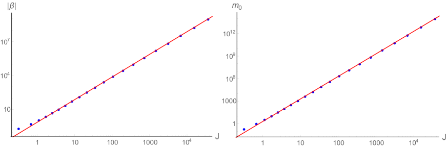
Figure 15: Left: $|\epsilon(J)|$ together with its fit to a $J^{2}$ power law. Right: $m_{0}(J)$ together with its fit to a $J^{3}$ power law.

B.3.2 The planar limit of the AdSJ branch

We are working with planar asymptotics now. Our first working hypothesis is that the planar geometry to which the soliton branch maps upon blow-up is Poincaré invariant. We also know that this putative solution is static and supported by a nontrivial scalar field profile, as its soliton progenitors. As a second working hypothesis, we are going to assume that this scalar field profile is monotonic, i.e., that

$$\phi^{\prime}(\chi)>0,$$ (B.48)

where $\chi$ is a suitable radial coordinate. This is natural to the extent that it also holds for the each individual solution in the soliton branch. Monotonicity implies that we can parameterize the radial direction in terms of $\phi$ itself, i.e., the implicit function theorem allows us to write $\chi=\chi(\phi)$.

These considerations motivate us to choose the metric ansatz

$$ds^{2}=e^{A(\phi)}(-dt^{2}+dx^{2}+dy^{2})+B(\phi)d\phi^{2}.$$ (B.49)

From the Einstein equation, we get that

$$B(\phi)=\frac{3A^{\prime}(\phi)^{2}-4}{4(3+2\phi^{2})},$$ (B.50)

$$A^{\prime\prime}(\phi)=\frac{(3+2\phi^{2}+\phi A^{\prime}(\phi))(-4+3A^{\prime}(\phi))}{6+4\phi^{2}},$$ (B.51)

while these relations automatically solve the scalar field equation.

In order to solve the equation of motion of $A$, we need to impose suitable boundary conditions. We know that the asymptotic UV region corresponds to the limit $\phi\to 0$, but what do the IR region corresponds to?

Regarding this point, note first that the planar solution must have zero entropy density, i.e., the area element of a constant time, constant $\phi$ hypesurface must tend to zero as such hypersurface tends to the far IR of the geometry. This implies that, as $\phi\to\phi_{IR}$, $A(\phi)$ must tend to $-\infty$. Here $\phi_{IR}$ is the value of the scalar field in the far IR of the geometry; at present we don’t wether $\phi_{IR}$ is finite or $\infty$.

In the case that $\phi_{IR}=\infty$, is easy to find a solution. If we assume that $A(\phi)\sim-\phi^{2}$ as $\phi\to\infty$, eq. (B.51) can be solved in a series expansion in inverse powers of $\phi$, together with an extra logarithmic contribution. Explicitly,

$$A(\phi)=-\phi^{2}-\frac{11}{3}\log\phi-\frac{11}{9\phi^{2}}+\frac{55}{27\phi^{4}}-\frac{671}{108\phi^{6}}+O\left(\frac{1}{\phi^{8}}\right).$$ (B.52)

Then, by eq. (B.50),

$$B(\phi)=\frac{3}{2}+\frac{11}{4\phi^{2}}-\frac{11}{4\phi^{4}}+\frac{77}{8\phi^{6}}+O\left(\frac{1}{\phi^{8}}\right).$$ (B.53)

In this case, $B$ is finite in the IR. From these series expansions, we clearly see that the IR solution is uniquely fixed and has no adjustable parameters. It should also be noted that this solution is singular in the IR. For instance, the Ricci scalar behaves as

$$R=-8\phi^{2}-\frac{32}{3}+O\left(\frac{1}{\phi^{2}}\right),$$ (B.54)

while the Kretschmann scalar as

$$K=\frac{32}{3}\phi^{4}+\frac{256}{9}\phi^{2}+\frac{760}{27}+O\left(\frac{1}{\phi^{2}}\right).$$ (B.55)

Is this singularity naked? To determine this, we must find out if there exists an apparent horizon in the solution. However, the series expansions are apparently not sufficient at this point: it seems that we need to find the full metric. This is not the case. We will show this by understanding better the IR geometry. In order to so, it is illustrative to change our coordinate system. From (B.49), we see that the Schwarzschild radial coordinate is given by

$$r(\phi)=e^{1/2A(\phi)}.$$ (B.56)

Note that, in particular, $r\to 0$ as $A\to-\infty$. To lowest nontrivial order in the $\phi\to\infty$ limit,

$$r(\phi)\sim\frac{e^{-\frac{1}{2}\phi^{2}}}{\phi^{\frac{11}{6}}},$$ (B.57)

from where we can solve for $\phi(r)$ in terms of the Lambert W function,

$$\phi(r)\sim\sqrt{\frac{11}{6}}\sqrt{W\left(\frac{6}{11r^{\frac{12}{11}}}\right)}.$$ (B.58)

This expression is only valid at leading order as $r\to 0$. In this limit, the argument of the W function diverges. Therefore, we can employ the leading order asymptotic expansion of W,

$$W(x)=\log x+O(\log\log x),$$ (B.59)

to get

$$\phi(r)\sim\sqrt{2}\sqrt{-\log r}.$$ (B.60)

Although $\phi$ diverges as $r\to 0$, this divergence is rather mild. In terms of the $r$ coordinate, $B(\phi)$ behaves as

$$B(r)=B(\phi(r))\sim 3/2$$ (B.61)

Therefore, at leading order, the $rr$-component of the metric tensor is

$$g_{rr}=B(r)\phi^{\prime}(r)^{2}\sim\frac{3}{4}\frac{1}{r^{2}(-\log r)}$$ (B.62)

and the whole metric asymptotes to the following IR geometry,

$$ds^{2}\sim r^{2}(-dt^{2}+d{\vec{x}}^{2})+\frac{dr^{2}}{\frac{4}{3}r^{2}(-\log r)}.$$ (B.63)

The scale invariance of the Poincaré patch is mildly broken by the $\log r$ term: only Poincaré invariance remains. Metrics of this kind have been previously found to be zero-temperature limits of holographic superconductors [HR]. Comparing this expression with the standard metric ansatz,

$$ds^{2}=-f(r)e^{-2\delta(r)}dt^{2}+\frac{dr^{2}}{f(r)}+r^{2}d\vec{x}^{2}$$ (B.64)

we see that

$$f(r)\sim-\frac{4}{3}r^{2}\log r,$$ (B.65)

$$\delta(r)\sim\frac{1}{2}\log\left(-\frac{4}{3}\log r\right).$$ (B.66)

In particular, $f(r=0)=0$, so the $r=0$ hypersurface corresponds to an apparent horizon. Therefore, the singularity is naked. It is also possible to compute the temperature associated to this horizon by the standard relation

$$T=\frac{1}{4\pi}\sqrt{f^{\prime}(r)\left(f(r)e^{-2\delta(r)}\right)^{\prime}}\bigg{\rvert}_{r=0}.$$ (B.67)

We get that, as $r\to 0$,

$$T\sim\frac{r\sqrt{-2\log r}}{\sqrt{6}\pi},$$ (B.68)

and so $T=0$. This solution has strict zero temperature. If the singular solution corresponds to the planar limit of the soliton branch, the Hawking-Page transition cannot have a planar limit. The reason is that the phase which dominates the grandcanonical ensemble in global AdS at low but finite temperatures maps to a zero temperature solution; in planar AdS, at any fixed and finite temperature, there is only one phase: the one that corresponds to the hairy black hole solutions. There are no competing saddles and no phase transition. This observation leads to the prediction that, when $J\to\infty$, $T_{HP}/J$ must vanish.

The previous discussion shows how important it is to find out whether the singular solution is the blow-up limit of the soliton branch. To do this, we solve (B.51) numerically by shooting from $\phi_{IR}\gg 1$ to $\phi_{UV}\ll 1$, using the IR series expansion of $A$ to provide the initial conditions for the shooting. Once $A(\phi)$ is known, $\phi(r),f(r)$ and $\delta(r)$ can be easily determined. Let us explain how.

Let us compactify the radial direction as usual, $r=\tan x$. Note that $x(\phi)=\arctan e^{1/2A(\phi)}$. In terms of $\phi$, we have that

$$f(\phi)=\sec^{2}(x(\phi))\tilde{f}(\phi),\tilde{f}(\phi)=\frac{e^{A(\phi)}(3+2\phi^{2})A^{\prime}(\phi)^{2}}{(1+e^{A(\phi)})(3A^{\prime}(\phi)^{2}-4)}$$ (B.69)

$$\delta(\phi)=\frac{1}{2}\log\frac{(3+2\phi^{2})A^{\prime}(\phi)^{2}}{3A^{\prime}(\phi)^{2}-4}.$$ (B.70)

where $\tilde{f}$ is analogous to the emblackening factor we have been using in the global case. Once these expressions are known, we interpolate $(x(\phi),\phi)$, $(x(\phi),\tilde{f}(\phi))$ and $(x(\phi),\delta(\phi))$. The results we have obtained are plotted in Fig.  16.

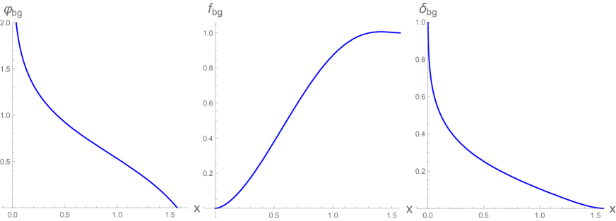
Figure 16: Metric and scalar field of the zero temperature solution

Once the background is known, we can compute the dimensionless ratios (B.44), with the result

$$\frac{\epsilon}{J^{2}}=0.7394,\leavevmode\nobreak\ \leavevmode\nobreak\ \leavevmode\nobreak\ \leavevmode\nobreak\ \leavevmode\nobreak\ \leavevmode\nobreak\ \frac{m_{0}}{J^{3}}=1.9741.$$ (B.71)

These ratios are extremely close to the values we have determined independently by analyzing the large $J$ behavior of $\epsilon$ and $m_{0}$ along the soliton branch. In particular, the relative difference between both $\hat{\epsilon}$’s is 0.081$\%$ , while the relative difference between both $\hat{m}_{0}$’s is 0.035$\%$: both quantities have a relative deviation smaller than $0.1\%$.

This establishes without a trace of doubt that the zero temperature planar solution we have constructed is the planar limit of the soliton branch, being the very small differences we observe due to accumulated numerical error.

According to our previous discussion, the fact that the planar limiting solution has strictly zero temperature implies that the Hawking-Page transition does not have a planar limit in this model. In particular, we must have that $\lim_{J\to\infty}T_{HP}/J=0$.

References

- [1] Robert C. Myers and Aninda Sinha. Holographic c-theorems in arbitrary dimensions. JHEP, 01:125, 2011.
- [2] E.T. Akhmedov. A remark on the ads/cft correspondence and the renormalization group flow. Physics Letters B, 442(1-4):152–158, Dec 1998.
- [3] Ofer Aharony, Steven S. Gubser, Juan Martin Maldacena, Hirosi Ooguri, and Yaron Oz. Large N field theories, string theory and gravity. Phys. Rept., 323:183–386, 2000.
- [4] Umut Gürsoy, Elias Kiritsis, Francesco Nitti, and Leandro Silva Pimenta. Exotic holographic rg flows at finite temperature. Journal of High Energy Physics, 2018(10), Oct 2018.
- [5] Edward Witten. Anti-de Sitter space, thermal phase transition, and confinement in gauge theories. Adv. Theor. Math. Phys., 2:505–532, 1998.
- [6] S. W. Hawking and D. N. Page. Thermodynamics of black holes in anti-de sitter space. Commun. Math. Phys. 87 (1983) 577, 1983.
- [7] Simon A. Gentle, Mukund Rangamani, and Benjamin Withers. A soliton menagerie in ads. Journal of High Energy Physics, 2012(5), May 2012.
- [8] Gary T. Horowitz and Robert C. Myers. Ads-cft correspondence and a new positive energy conjecture for general relativity. Phys. Rev. D, 59:026005, Dec 1998.
- [9] Sean A. Hartnoll, Christopher P. Herzog, and Gary T. Horowitz. Holographic Superconductors. JHEP, 12:015, 2008.
- [10] Pallab Basu, Jyotirmoy Bhattacharya, Sayantani Bhattacharyya, R. Loganayagam, Shiraz Minwalla, and V. Umesh. Small Hairy Black Holes in Global AdS Spacetime. JHEP, 10:045, 2010.
- [11] Óscar J. C. Dias, Pau Figueras, Shiraz Minwalla, Prahar Mitra, Ricardo Monteiro, and Jorge E. Santos. Hairy black holes and solitons in global ads5. Journal of High Energy Physics, 2012(8), Aug 2012.
- [12] Pallab Basu, Jyotirmoy Bhattacharya, and Sayan Kumar Das. A holographic superconductor forced through interactions. JHEP, 08:089, 2019.
- [13] Sean A. Hartnoll, Andrew Lucas, and Subir Sachdev. Holographic quantum matter. 12 2016.
- [14] Franz E. Schunck and Eckehard W. Mielke. TOPICAL REVIEW: General relativistic boson stars. Classical and Quantum Gravity, 20(20):R301–R356, October 2003.
- [15] John Archibald Wheeler. Geons. Phys. Rev., 97:511–536, Jan 1955.
- [16] David J. Kaup. Klein-Gordon Geon. Physical Review, 172(5):1331–1342, August 1968.
- [17] Dumitru Astefanesei and Eugen Radu. Boson stars with negative cosmological constant. Nucl. Phys. B, 665:594–622, 2003.
- [18] Kevin Goldstein, Norihiro Iizuka, Rudra P. Jena, and Sandip P. Trivedi. Nonsupersymmetric attractors. Physical Review D, 72(12), Dec 2005.
- [19] Shinsei Ryu and Tadashi Takayanagi. Holographic derivation of entanglement entropy from the anti–de sitter space/conformal field theory correspondence. Physical Review Letters, 96(18), May 2006.
- [20] Ioannis Bakas and Georgios Pastras. Entanglement entropy and duality in ads4. Nuclear Physics B, 896:440–469, 2015.
- [21] Ofer Aharony, Joseph Marsano, Shiraz Minwalla, Kyriakos Papadodimas, and Mark Van Raamsdonk. The deconfinement and hagedorn phase transitions in weakly coupled large n gauge theories. Comptes Rendus Physique, 5(9-10):945–954, Nov 2004.
- [22] Edward Witten. Multi-Trace Operators, Boundary Conditions, And AdS/CFT Correspondence. arXiv e-prints, pages hep–th/0112258, December 2001.
- [23] Eric D’Hoker and Per Kraus. Magnetic brane solutions in ads. Journal of High Energy Physics, 2009(10):088–088, Oct 2009.
- [24] Gary T. Horowitz, Jorge E. Santos, and David Tong. Optical conductivity with holographic lattices. Journal of High Energy Physics, 2012(7), Jul 2012.
- [25] Current authors. Confinement and incomplete holographic rg flow.
- [26] Kirill Bronnikov. Scalar fields as sources for wormholes and regular black holes. Particles, 1(1):5, Mar 2018.
- [27] Juan Maldacena, Alexey Milekhin, and Fedor Popov. Traversable wormholes in four dimensions, 2020.