Limit of connected multigraph with fixed degree sequence

Abstract

Motivated by the scaling limits of the connected components of the configuration model, we study uniform connected multigraphs with fixed degree sequence $\mathcal{D}$ and with surplus $k$. We call those random graphs $(\mathcal{D},k)$-graphs. We prove that, for every $k\in\mathbb{N}$, under natural conditions of convergence of the degree sequence, ($\mathcal{D},k)$-graphs converge toward either $(\mathcal{P},k)$-graphs or $(\Theta,k)$-ICRG (inhomogeneous continuum random graphs). We prove similar results for $(\mathcal{P},k)$-graphs and $(\Theta,k)$-ICRG, which have applications to multiplicative graphs. Our approach relies on two algorithms, the cycle-breaking algorithm, and the stick-breaking construction of $\mathcal{D}$-tree that we introduced in a recent paper. From those algorithms we deduce a biased construction of $(\mathcal{D},k)$-graph, and we prove our results by studying this bias.

1 Introduction

The present work is a continuation of our previous paper [12], where we introduced a stick-breaking construction for $\mathcal{D}$-trees (uniform tree with fixed degree sequence $\mathcal{D}$) to prove that, under natural conditions, $\mathcal{D}$-trees converge, in a GP and a GHP sens, toward either $\mathcal{P}$-trees or ICRT. Here, we derive from [12] similar limits for graph versions of those trees, which have applications to multiplicative graphs and to the configuration model.

1.1 Motivations

Computer scientists have introduced multiplicative graphs [22, 30, 16] and the configuration model [9, 14] as natural generalizations of the Erdős–Rényi model. They are studied for 2 main reasons: first many tools introduced for the Erdős–Rényi model can also be used to study those graphs, then those models seems closer to real life network thanks to the "inhomogeneity in their degree distribution" (see e.g. Newman [29]). For those reasons, they are currently great models to study the evolution of random networks.

A natural question for any model of evolution is to study their potential phase transitions. It appears that those graphs have an intriguing phase transition where a giant component gets born. We refer the reader to [24] Chapter 1 and references therein for an elaborate discussion of the nature of this transition, and an overview of the literature it generated.

From the point of view of precise asymptotics, a main goal is to study the geometry of the connected components of those graphs in the critical regime. To this end, Addario-Berry, Broutin, and Goldschmidt [2] have developed a general approach in the case of the Erdős–Rényi model. This approach is divided in two main steps:

• First one encodes the random graphs into stochastic processes, and study those processes to deduce several limits for relevant quantities of the largest connected components such as the size, surplus, degrees. This has been noticed in the ground-breaking work of Aldous [7].

• Then, one use those convergences to reduce the problem to a study of a single connected component conditioned on those quantities.

This approach has been further developed for multiplicative graphs and the configuration model in many different regimes. We refer the reader to [2, 11, 10] for the homogeneous case, [23, 25, 26] for the power law case, and [18, 19] for a unified approach for multiplicative graphs. In this paper, we focus on solving (b), under what we believe to be the weakest assumptions. So we reduce the study of the largest connected components to solving (a), which tends to be simpler.

Moreover, we give a universal point of view on those models which can be summarized into the three following points: we describe multiplicative graphs as degenerate configuration model, we extend the unified point of view of Broutin, Duquesne, and Minmin [18, 19] to the configuration model, and we remove the omnipresent randomness assumption in the degree sequence.

1.2 Overview of the proof

Fix $k\in\mathbb{N}$. Fix $\{V_{i}\}_{i\in\mathbb{N}}$ a set of vertices. We say that a multigraph $G$ have degree sequence $\mathcal{D}=(d_{1},\dots,d_{s})$ if $G$ has vertices $(V_{1},\dots,V_{s})$ and for every $1\leq i\leq s$, $V_{i}$ has degree $d_{i}+1$. (This shift of $+1$ will be convenient to simplify many expressions, and to be coherent with [12].) The surplus of a connected multigraph $(V,E)$ is $|E|-|V|+1$, and is, informally, the number of edges that one needs to delete to transform a multigraph into a tree. A $(\mathcal{D},k)$-graph is a uniform connected multigraph with degree sequence $\mathcal{D}$ and surplus $k$.

Our goal is to study the connected components of the configuration model conditioned on having degree sequence $\mathcal{D}$ and surplus $k$, which are close from $(\mathcal{D},k)$-graphs (see Lemma 8.3). To this end, we rely on two algorithms: the stick-breaking construction of $\mathcal{D}$-trees of [12], along with the cycle-breaking algorithm introduced by Addario-Berry, Broutin, Goldschmidt, and Miermont [3] which we invert to construct $(\mathcal{D},k)$-graph by adding $k$ edges to a biased $\mathcal{D}$-tree.

We use the cycle breaking algorithm in the following form. Take a connected multigraph with surplus $k$, repeat $k$ times: choose an edge uniformly among all the edges that can be removed without disconnecting the graph, then cut this edge in the middle. By doing so, we add $2k$ named leaves $(\star_{i})_{1\leq i\leq 2k}$, and keep the degrees of $(V_{i})_{i\in\mathbb{N}}$. Note that to invert this algorithm we can intuitively repair the broken edges by gluing the different pairs in $(\star_{i})_{1\leq i\leq 2k}$. Note that however this algorithm is not a bijection, since for each multigraph there are many corresponding trees. To bypass this, we bias each tree by the probability that they were obtained by their corresponding multigraph. This way, we construct a $(\mathcal{D},k)$-graph from a biased $\mathcal{D}$-tree with $k$ additional edges.

Thus, to study the geometry of a $(\mathcal{D},k)$-graph, it is enough to study jointly the geometry of a $\mathcal{D}$-tree, the positions of $(\star_{i})_{1\leq i\leq 2k}$, and the previous bias which is a function of $(d(\star_{i},\star_{j}))_{1\leq i,j\leq 2k}$. Therefore, it is enough to study precisely the distance matrix between specific vertices of a $\mathcal{D}$-tree. If the bias was a continuous function of this matrix, then our main results would directly follow from [12] since the GP convergence of $\mathcal{D}$-trees implies the convergence of this matrix. However, some extra care is needed since the bias diverges when $(\star_{i})_{1\leq i\leq 2k}$ are close.

Therefore, we need to prove that $(\star_{i})_{1\leq i\leq 2k}$ cannot be too close. More precisely we show, using the structure of $\mathcal{D}$-trees and of the bias, that it is enough to lower bound $(d(\star_{0},\star_{i}))_{1\leq i\leq k}$ where $\star_{0}$ is a root leaf. We then use our construction of $\mathcal{D}$-trees, also introduced independently by Addario-Berry, Donderwinkel, Maazoun, and Martin in [4], to lower bound those distances using the $k$ first repetitions in a random tuple.

Finally, since the bias is a function of the subtree spanned by $(\star_{i})_{1\leq i\leq 2k}$, it is also a function of the first branches of the stick-breaking construction. This allows us to consider the limit of the bias, to directly construct the limits of $(\mathcal{D},k)$-graphs by biasing the $\mathcal{P}$-trees and ICRT, introduced by Aldous, Camarri and Pitman [8, 21], and then by gluing the $k$ first pair of leaves.

Plan of the paper:

In Section 2 we introduce the topologies that we are using in this paper. In Section 3, we construct $\mathcal{D}$-trees, $\mathcal{P}$-trees, and $\Theta$-ICRT. In Section 4, we construct $(\mathcal{D},k)$-graphs, $(\mathcal{P},k)$-graphs, and $(\Theta,k)$-ICRG. We state our main results in Section 5. We study the bias in section 6. We deduce our main results in Section 7. Finally we discuss in Section 8 some connections between $(\mathcal{D},k)$-graph, $(\mathcal{P},k)$-graphs, the configuration model and multiplicative graphs.

Notations:

Throughout the paper, similar variables for, $\mathcal{D}$-trees, $(\mathcal{D},k)$-graphs, $\mathcal{P}$-trees, $(\mathcal{P},k)$-graphs, $\Theta$-ICRT, $(\Theta,k)$-ICRG share similar notations. To avoid any ambiguity, the models that we are using and their parameters are indicated by superscripts $\mathcal{D}$, $(\mathcal{D},k)$, $\mathcal{P}$ ,$(\mathcal{P},k)$, $\Theta$, $(\Theta,k)$. We often drop those superscripts when the context is clear.

Acknowledgment

Thanks are due to Nicolas Broutin for many advices on the configuration model and on multiplicative graphs.

2 Notions of convergence

2.1 Gromov–Prokhorov (GP) topology

A measured metric space is a triple $(X,d,\mu)$ such that $(X,d)$ is a Polish space and $\mu$ is a Borel probability measure on $X$. Two such spaces $(X,d,\mu)$, $(X^{\prime},d^{\prime},\mu^{\prime})$ are called isometry-equivalent if there exists an isometry $f:X\to X^{\prime}$ such that if $f_{\star}\mu$ is the image of $\mu$ by $f$ then $f_{\star}\mu=\mu^{\prime}$. Let $\mathbb{K}_{\text{GP}}$ be the set of isometry-equivalent classes of measured metric space. Given a measured metric space $(X,d,\mu)$, we write $[X,d,\mu]$ for the isometry-equivalence class of $(X,d,\mu)$ and frequently use the notation $X$ for either $(X,d,\mu)$ or $[X,d,\mu]$.

We now recall the definition of the Prokhorov’s distance. Consider a metric space $(X,d)$. For every $A\subset X$ and $\varepsilon>0$ let $A^{\varepsilon}:=\{x\in X,d(x,A)<\varepsilon\}$. Then given two (Borel) probability measures $\mu$, $\nu$ on $X$, the Prokhorov distance between $\mu$ and $\nu$ is defined by

$$d_{P}(\mu,\nu):=\inf\{\text{ $\varepsilon>0$: $\mu\{A\}\leq\nu\{A^{\varepsilon}\}$ and $\nu\{A\}\leq\mu\{A^{\varepsilon}\}$, for all Borel set $A\subset X$}\}.$$

The Gromov–Prokhorov (GP) distance is an extension of the Prokhorov’s distance: For every $(X,d,\mu),(X^{\prime},d^{\prime},\mu^{\prime})\in\mathbb{K}_{\text{GP}}$ the Gromov–Prokhorov distance between $X$ and $X^{\prime}$ is defined by

$$d_{\text{GP}}((X,d,\mu),(X^{\prime},d^{\prime},\mu^{\prime})):=\inf_{S,\phi,\phi^{\prime}}d_{P}(\phi_{\star}\mu,\phi^{\prime}_{\star}\mu^{\prime}),$$

where the infimum is taken over all metric spaces $S$ and isometric embeddings $\phi:X\to S$, $\phi^{\prime}:X^{\prime}\to S$. $d_{\text{GP}}$ is indeed a distance on $\mathbb{K}_{\text{GP}}$ and $(\mathbb{K}_{\text{GP}},d_{\text{GP}})$ is a Polish space (see e.g. [1]).

We use another convenient characterization of the GP topology: For every measured metric space $(X,d^{X},\mu^{X})$ let $(x_{i}^{X})_{i\in\mathbb{N}}$ be a sequence of i.i.d. random variables of common distribution $\mu^{X}$ and let $M^{X}:=(d^{X}(x_{i}^{X},x_{j}^{X}))_{(i,j)\in\mathbb{N}^{2}}$. We prove the following result in [12] (see also [28]),

Lemma 2.1.

Let $(X^{n})_{n\in\mathbb{N}}\in\mathbb{K}_{\text{GP}}^{\mathbb{N}}$ and let $X\in\mathbb{K}_{\text{GP}}$. Let $(y^{X}_{i})_{i\in\mathbb{N}}$ be a sequence of random variables on $X$ and let $N^{X}:=(d^{X}(y_{i}^{X},y_{j}^{X}))_{(i,j)\in\mathbb{N}^{2}}$. If

$$M^{X_{n}}\operatorname*{\longrightarrow}^{(d)}N^{X}\quad\text{and}\quad\frac{1}{n}\sum_{i=1}^{n}\delta_{y^{X}_{i}}\operatorname*{\longrightarrow}^{(d)}\mu^{X},$$

then $X^{n}\operatorname*{\longrightarrow}^{\text{GP}}X$.

2.2 Gromov–Hausdorff (GH) topology

Let $\mathbb{K}_{\text{GH}}$ be the set of isometry-equivalent classes of compact metric space. For every metric space $(X,d)$, we write $[X,d]$ for the isometry-equivalent class of $(X,d)$, and frequently use the notation $X$ for either $(X,d)$ or $[X,d]$.

For every metric space $(X,d)$, the Hausdorff distance between $A,B\subset X$ is given by

$$d_{H}(A,B):=\inf\{\varepsilon>0,A\subset B^{\varepsilon},B\subset A^{\varepsilon}\}.$$

The Gromov–Hausdorff distance between $(X,d)$,$(X^{\prime},d^{\prime})\in\mathbb{K}_{\text{GH}}$ is given by

$$d_{\text{GH}}((X,d),(X^{\prime},d^{\prime})):=\inf_{S,\phi,\phi^{\prime}}\left(d_{H}(\phi(X),\phi^{\prime}(X^{\prime}))\right),$$

where the infimum is taken over all metric spaces $S$ and isometric embeddings $\phi:X\to S$, $\phi^{\prime}:X^{\prime}\to S$. $d_{\text{GH}}$ is indeed a distance on $\mathbb{K}_{\text{GH}}$ and $(\mathbb{K}_{\text{GH}},d_{\text{GH}})$ is a Polish space (see e.g. [1]).

2.3 Pointed Gromov–Hausdorff ($\text{GH}^{n}$) topology

Let $n\in\mathbb{N}$. Let $(X,d,(x_{1},\dots,x_{n}))$ and $(X^{\prime},d^{\prime},(x^{\prime}_{1},\dots,x^{\prime}_{n}))$ be metric spaces, each equiped with an ordered sequence of $n$ distinguished points (we call such spaces $n$-pointed metric spaces). We say that these two $n$-pointed metric spaces are isometric if there exists an isometry $\phi$ from $(X,d)$ on $(X^{\prime},d^{\prime})$ such that for every $1\leq i\leq n$, $\phi(x_{i})=x^{\prime}_{i}$.

Let $\mathbb{K}^{n}_{\text{GH}}$ be the set of isometry-equivalent classes of compact metric space. As before, we write $[X,d,(x_{1},x_{2},\dots,x_{n})]$ for the isometry-equivalent class of $(X,d,(x_{1},\dots,x_{n}))$, and denote either by $X$ when there is little chance of ambiguity.

The $n$-pointed Gromov–Hausdorff distance between $X,X^{\prime}\in\mathbb{K}^{n}_{\text{GH}}$ is given by

$$d_{\text{GH}}^{n}((X,d,(x_{1},\dots,x_{n})),(X^{\prime},d^{\prime},(x^{\prime}_{1},\dots,x^{\prime}_{n}))):=\inf_{S,\phi,\phi^{\prime}}\left(d_{H}(\phi(X),\phi^{\prime}(X^{\prime}))\right),$$

where the infimum is taken over all metric spaces $S$ and isometric embeddings $\phi:X\to S$, $\phi^{\prime}:X^{\prime}\to S$ such that for every $1\leq i\leq n$, $\phi(x_{i})=\phi^{\prime}(x^{\prime}_{i})$. $d^{n}_{\text{GH}}$ is indeed a distance on $\mathbb{K}^{n}_{\text{GH}}$ and $(\mathbb{K}^{n}_{\text{GH}},d^{n}_{\text{GH}})$ is a Polish space (see [3] Section 2.1).

2.4 Extension to pseudo metric spaces

Note that the previous topologies naturally extends to pseudo metric spaces. Indeed, one may say that a pseudo metric space $(X,d)$ is isometry-equivalent to the metric space given by quotienting $X$ by the equivalent relation $d(a,b)=0$ (see Burago, Burago, Ivanov [20] for details.) It is then enough to extend the equivalent classes to pseudo metric spaces.

3 Constructions of $\mathcal{D}$-trees, $\mathcal{P}$-trees and $\Theta$-ICRT

3.1 $\mathcal{D}$-trees

Recall that a sequence $(d_{1},\dots,d_{s})$ is a degree sequence of a tree if and only if $\sum_{i=1}^{s}d_{i}=s-2$, and by convention $d_{1}\geq d_{2}\dots\geq d_{s}$. Let $\Omega_{\mathcal{D}}$ be the set of such sequences.

For convenience issue, we want to label our leaves on a set $\{\star_{i}\}_{i\in\mathbb{N}}$ disjoint from $\{V_{i}\}_{i\in\mathbb{N}}$. So let us slightly change our definition of $\mathcal{D}$-trees. Note that a tree with degree sequence $\mathcal{D}$ must have $N^{\mathcal{D}}+2:=\sum_{i=1}^{s}\mathbf{1}_{d_{i}=0}$ leaves. We say that a tree $T$ is a $\mathcal{D}$-tree if it is uniform among all tree with vertices $\{V_{i}\}_{i:d_{i}>0}\cup\{\star_{i}\}_{0\leq i\leq N+1}$ and such that for every $i$ with $d_{i}>0$, $\deg(V_{i})=d_{i}+1$.

We now recall the construction of $\mathcal{D}$-trees of [12]. For simplicity, for every graph $G=(V,E)$ and edge $e=\{v_{1},v_{2}\}$, $G\cup e$ denotes the graph $(V\cup\{v_{1},v_{2}\},E\cup\{e\})$.

Algorithm 1 (Algorithm 7 from [12]).

Stick-breaking construction of a $\mathcal{D}$-tree $T^{\mathcal{D}}$ (see Figure 1).

• Let $A^{\mathcal{D}}=(A^{\mathcal{D}}_{i})_{1\leq i\leq s-1}$ be a uniform $\mathcal{D}$-tuple (tuple such that $\forall i\in\mathbb{N}$, $V_{i}$ appears $d_{i}$ times).

• Let $T^{\mathcal{D}}_{1}:=(\{\star_{0},A_{1}\},\{\{\star_{0},A_{1}\}\})$ then for every $2\leq i\leq s$ let

  $$T^{\mathcal{D}}_{i}:=\begin{cases}T_{i-1}\cup\{A_{i-1},A_{i}\}&\text{if }A_{i}\notin T_{i-1}.\\ T_{i-1}\cup\{A_{i-1},\star_{\inf\{k,\star_{k}\notin T_{i-1}\}}\}&\text{if }A_{i}\in T_{i-1}\text{ or }i=s.\end{cases}$$

• Let $T^{\mathcal{D}}=T_{s}$.

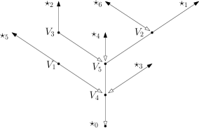
Figure 1: Stick breaking construction of a $\mathcal{D}$-tree with $\mathcal{D}=(1,2,1,3,3,0,0,\dots)$ and $(A^{\mathcal{D}}_{i})_{1\leq i\leq s-1}=(V_{4},V_{5},V_{2},V_{5},V_{3},V_{4},V_{5},V_{4},V_{1},V_{2})$. The exploration starts at $\star_{0}$ then follows the white-black arrow toward $\star_{1}$, then jumps at $\star_{5}$ to follow the path toward $\star_{2}$ and so on…

3.2 $\mathcal{P}$-trees

Let $\{V_{\infty,i}\}_{i\in\mathbb{N}}$ be a set of vertices disjoint with $\{V_{i}\}_{i\in\mathbb{N}}$ and $\{\star_{i}\}_{i\geq 0}$. Let $\Omega_{\mathcal{P}}$ be the set of sequence $(p_{i})_{i\in\mathbb{N}\cup\{\infty\}}$ in $\mathbb{R}^{+}$ such that $\sum_{i=1}^{\infty}p_{i}+p_{\infty}=1$, $p_{1}>0$ and $p_{1}\geq p_{2}\geq\dots$. For every $\mathcal{P}\in\Omega_{\mathcal{P}}$, the $\mathcal{P}$-tree is the random tree constructed as follow:

Algorithm 2.

Definition of the $\mathcal{P}$-tree for $\mathcal{P}\in\Omega_{\mathcal{P}}$.

• Let $(A^{\mathcal{P}}_{i})_{i\in\mathbb{N}}$ be a family of i.i.d. random variables such that for all $i\in\mathbb{N}$, $\mathbb{P}(A^{\mathcal{P}}_{1}=V_{i})=p_{i}$.

• For every $i\in\mathbb{N}$, let $B^{\mathcal{P}}_{i}=A_{i}$ if $A_{i}\in\mathbb{N}$, and let $B^{\mathcal{P}}_{i}=V_{\infty,i}$ otherwise.

• Let $T^{\mathcal{P}}_{1}:=(\{\star_{0},B_{1}\},\{\{\star_{0},B_{1}\}\})$ then for every $i\geq 2$ let

  $$T^{\mathcal{P}}_{i}:=\begin{cases}T_{i-1}\cup\{B_{i-1},B_{i}\}&\text{if }B_{i}\notin T_{i-1}.\\ T_{i-1}\cup\{B_{i-1},\star_{\inf\{k,\star_{k}\notin T_{i-1}\}}\}&\text{if }B_{i}\in T_{i-1}.\end{cases}$$

• Let $T^{\mathcal{P}}:=\bigcup_{n\in\mathbb{N}}T_{n}$.

Remark.

Usually, the leaves $\{\star_{i}\}_{i\in\mathbb{N}}$ are omitted in the formal definition of $\mathcal{P}$-trees. We consider them to clarify the intuition that they are degenerate $\mathcal{D}$-trees with an infinite number of leaves.

3.3 ICRT

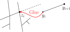
Figure 2: A typical step of the stick-breaking construction: the "gluing" of $(y_{i},y_{i+1}]$ at $z_{i}$.

First let us introduce a generic stick breaking construction. It takes for input two sequences in $\mathbb{R}^{+}$ called cuts ${\textbf{y}}=(y_{i})_{i\in\mathbb{N}}$ and glue points ${\textbf{z}}=(z_{i})_{i\in\mathbb{N}}$, which satisfy

$$\forall i<j,\ \ y_{i}<y_{j}\qquad;\qquad y_{i}\operatorname*{\longrightarrow}\infty\qquad;\qquad\forall i\in\mathbb{N},\ \ z_{i}\leq y_{i},$$ (1)

and creates a $\mathbb{R}$-tree (loopless geodesic metric space) by recursively "gluing" segment $(y_{i},y_{i+1}]$ on position $z_{i}$, or rigorously, by constructing a consistent sequence of distances $(d_{n})_{n\in\mathbb{N}}$ on $([0,y_{n}])_{n\in\mathbb{N}}$.

Algorithm 3.

Generic stick-breaking construction of $\mathbb{R}$-tree.

• Let $d_{0}$ be the trivial metric on $[0,0]$.

• For each $i\geq 0$ define the metric $d_{i+1}$ on $[0,y_{i+1}]$ such that for each $x\leq y$:

  $$d_{i+1}(x,y):=\begin{cases}d_{i}(x,y)&\text{if }x,y\in[0,y_{i}]\\ d_{i}(x,z_{i})+|y-y_{i}|&\text{if }x\in[0,y_{i}],\,y\in(y_{i},y_{i+1}]\\ |x-y|&\text{if }x,y\in(y_{i},y_{i+1}],\end{cases}$$

  where by convention $y_{0}:=0$ and $z_{0}:=0$.

• Let $d$ be the unique metric on $\mathbb{R}^{+}$ which agrees with $d_{i}$ on $[0,y_{i}]$ for each $i\in\mathbb{N}$.

• Let $\operatorname*{SB}({\textbf{y}},{\textbf{z}})$ be the completion of $(\mathbb{R}^{+},d)$.

Now, let $\Omega_{\Theta}$ be the space of sequences $(\theta_{i})_{i\in\{0\}\cup\mathbb{N}}$ in $\mathbb{R}^{+}$ such that $\sum_{i=0}^{\infty}\theta_{i}^{2}=1$ and such that $\theta_{1}\geq\theta_{2}\geq\dots$. For every $\Theta\in\Omega_{\Theta}$, the $\Theta$-ICRT is the random $\mathbb{R}$-tree constructed as follow:

Algorithm 4.

Construction of $\Theta$-ICRT (from [13])

• Let $(X_{i})_{i\in\mathbb{N}}$ be a family of independent exponential random variables of parameter $(\theta_{i})_{i\in\mathbb{N}}$.

• Let $\mu$ be the measure on $\mathbb{R}^{+}$ defined by $\mu=\theta_{0}^{2}dx+\sum_{i=1}^{\infty}\delta_{X_{i}}\theta_{i}$.

• Let $(Y_{i},Z_{i})_{i\in\mathbb{N}}$ be a Poisson point process on $\{(y,z)\in\mathbb{R}^{+2}:y\geq z\}$ of intensity $dy\times d\mu$.

• Let $\textbf{Y}:=(Y_{i})_{i\in\mathbb{N}}$ and let $\textbf{Z}:=(Z_{i})_{i\in\mathbb{N}}$. Let $(Y_{0},Z_{0}):=(0,0)$.

• The $\Theta$-ICRT is defined as $(T,d)=\operatorname*{SB}(\textbf{Y},\textbf{Z})$. (see Algorithm 3)

4 Constructions of $(\mathcal{D},k)$-graphs, $(\mathcal{P},k)$-graphs and $(\Theta,k)$-ICRG

4.1 Generic gluing and cycle-breaking of discrete multigraphs (see Figure 3)

In the entire section, $G=(V,E)$ denotes a multigraph. Let $\operatorname*{cyc}(G)$ the set of all edges $e\in E$ such that $G\backslash\{e\}:=(V,E\backslash\{e\})$ is connected. (For multiples edges the operation $\backslash$ only remove one edge at a time.) Let $\square(G):=\#\operatorname*{cyc}(G)$.

For every leaves $L_{1}\neq L_{2}\in G$, we define the operation of gluing $L_{1}$ and $L_{2}$ in $G$ as follow: For every leaf $L\in G$, let the father of $L$ be the only vertex $F\in G$ such that $(F,L)\in G$. Let $F_{1}$, $F_{2}$ be the father of $L_{1},L_{2}$. The multigraph obtained by gluing $L_{1}$ and $L_{2}$ in $G$ is

$$\mathcal{G}_{L_{1},L_{2}}(G):=(V/\{L_{1},L_{2}\},E\backslash\{\{F_{1},L_{1}\},\{F_{2},L_{2}\}\}\cup\{\{F_{1},F_{2}\}\}),$$

and intuitively corresponds to the graph obtained by fusing $\{F_{1},L_{1}\}$ and $\{F_{2},L_{2}\}$.

Similarly, for every leaves $L_{1}\neq L_{2}\neq\dots,L_{2k-1}\neq L_{2k}$, the multigraph obtained by gluing $L_{1}$ and $L_{2}$,…, $L_{2k-1}$ and $L_{2k}$ in $G$ is

$$\mathcal{G}_{(L_{i})_{1\leq i\leq 2k}}(G)=\mathcal{G}_{(L_{1},L_{2}),(L_{3},L_{4})\dots,(L_{2k-1},L_{2k})}(G):=\mathcal{G}_{L_{1},L_{2}}\circ\mathcal{G}_{L_{3},L_{4}}\circ\dots\circ\mathcal{G}_{L_{2k-1},L_{2k}}(G).$$

Note that this multigraph does not depend on the order in which we glue the different leaves.

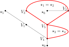
Figure 3: Gluing leaves of the tree $T$ from Figure 1 to form a graph $G$ with surplus 2. $\operatorname*{cyc}(G)$ is red. $\square(G)=5$. $G=\mathcal{G}_{(\star_{1},\star_{2},\star_{3},\star_{4})}(T)$. Also, $\mathbb{P}(\operatorname*{CB}(G)=T)=\frac{2!}{2^{2}\square(G\backslash\{V_{4},V_{5}\})\square(G)}=\frac{2}{2^{2}*3*5}$.

Now recall Section 1.2. Let us give a formal definition of the cycle-breaking algorithm:

Algorithm 5.

Cycle-breaking of a multigraph $G=(V,E)$ with $V\subset(V_{i})_{i\in\mathbb{N}}$ and surplus $k$.

• For $1\leq i\leq k$, let $e_{i}=(W_{2i+1},W_{2i+2})$ be a uniform oriented edge in $\operatorname*{cyc}(G\backslash\{e_{j}\}_{1\leq j<i})$.

• Let $\operatorname*{CB}(G):=(V\cup\{\star_{i}\}_{1\leq i\leq k},(E\backslash\{e_{i}\}_{1\leq i\leq k})\cup\{\{W_{i},\star_{2k+1-i}\}\}_{1\leq i\leq 2k})$.

To simplify our notations for every multigraph $G=(V,E)$ and $v,w\in V$, we write $\#_{v,w}(G)$ for the number of edges $\{v,w\}$ in $G$. Also, let $\circ(G):=\prod_{v\in V}2^{\#_{v,v}(G)}\prod_{v,w\in V}\#_{v,w}(G)!$.

Lemma 4.1.

For every connected multigraph $G$ with $V\subset\{V_{i}\}_{i\in\mathbb{N}}$ and surplus $k$, we have:

• $\operatorname*{CB}(G)$ is almost surely a tree with vertices $V\cup\{\star_{i}\}_{1\leq i\leq 2k}$.

• For every $v\in V$, $\deg_{\operatorname*{CB}(G)}(v)=\deg_{G}(v)$. For every $1\leq i\leq 2k$, $\star_{i}$ is a leaf in $\operatorname*{CB}(G)$.

• Almost surely, $\mathcal{G}_{(\star_{1},\star_{2}),\dots,(\star_{2k-1},\star_{2k})}(\operatorname*{CB}(G))=G$.

• For every tree $T$ satisfying (a) (b),

  $$\mathbb{P}(\operatorname*{CB}(G)=T)=\frac{\circ(G)}{2^{k}\prod_{i=1}^{k}\square(G\backslash\{e_{j}\}_{1\leq j<i})}.$$ (2)

Proof.

(a) and (b) follows from a quick enumeration. (c) is easy to prove from the definition of $\mathcal{G}$. (d) follows from an induction. Indeed, the right hand side of (2) is just the product over each steps of the probability that $(W_{2i+1},W_{2i+2})$ satisfies $\{W_{2i+1},\star_{2k-2i}\},\{W_{2i+2},\star_{2k-2i-1}\}\in T$. ∎

4.2 $(\mathcal{D},k)$-graph

Note that $(d_{1},\dots,d_{s})$ is a degree sequence of a connected multigraph with surplus $k$ if and only if $\sum_{i=1}^{s}d_{i}=s+k-2$, and by convention $d_{1}\geq d_{2}\dots\geq d_{s}$. Note that by adding $2k$ numbers $0$, this holds if and only if $(d_{1},\dots,d_{s},0,\dots,0)\in\Omega_{\mathcal{D}}$.

For convenience issue, let us slightly extend our definition of $(\mathcal{D},k)$-graph. For $\mathcal{D}\in\Omega_{\mathcal{D}}$ with $N^{\mathcal{D}}\geq 2k$ we say that $G$ is a $(\mathcal{D},k)$-graph if it is uniform among all multigraph with vertices $\{V_{i}\}_{i:d_{i}>0}\cup\{\star_{i}\}_{i\in\{0\}\cup\{2k+1,\dots,N^{\mathcal{D}}+1\}}$ and such that for every $i$ with $d_{i}>0$, $\deg(V_{i})=d_{i}+1$. The following result follows from Lemma 4.1 and constructs a $(\mathcal{D},k)$-graph from a biased $\mathcal{D}$-tree.

Lemma 4.2.

Let $T^{\mathcal{D},k}$ be a random tree. Assume that for every tree $T$ such that: T have vertices $\{V_{i}\}_{1\leq i\leq s}\cup\{\star_{i}\}_{1\leq i\leq 2k}$, for every $1\leq i\leq s$ $\deg_{T}(V_{i})=d_{i}+1$, and $\{\star_{i}\}_{1\leq i\leq 2k}$ are leaves of $T$,

$$\mathbb{P}(T^{\mathcal{D},k}=T)\alpha\frac{\circ(\mathcal{G}_{(\star_{i})_{1\leq i\leq 2k}}(T))}{\prod_{i=1}^{k}\square(\mathcal{G}_{(\star_{1},\star_{2}),\dots,(\star_{2i-1},\star_{2i})}(T))},$$ (3)

where $\alpha$ stands for proportional. Then $\mathcal{G}_{(\star_{i})_{1\leq i\leq 2k}}(T^{\mathcal{D},k})$ is a $(\mathcal{D},k)$-graph.

To simplify our notations, we write for every $i\in\mathbb{N}$, $\square_{i}(\cdot):=\square(\mathcal{G}_{(\star_{1},\star_{2}),\dots,(\star_{2i-1},\star_{2i})}(\cdot))$ and $\square_{\square,k}(\cdot):=\circ(\mathcal{G}_{(\star_{i})_{1\leq i\leq 2k}}(T))/\prod_{i=1}^{k}\square_{i}(\cdot)$. So that the right hand side of (3) is $\square_{\square,k}(T)$.

4.3 $(\mathcal{P},k)$-graph

Since $\mathcal{P}$-trees appear at the limit of $\mathcal{D}$-trees, it is natural to adapt Lemma 4.2 to construct limits for $(\mathcal{D},k)$-graphs from $\mathcal{P}$-trees. Thus we informally define the $(\mathcal{P},k)$-graph as a $\mathcal{P}$-tree biased by (2) where we glued $\{\star_{2i-1},\star_{2i}\}_{1\leq i\leq k}$. Below we formally define $(\mathcal{P},k)$-graph.

Fix $\mathcal{P}\in\Omega_{\mathcal{P}}$. First note that Algorithm 2 can be seen as a function AB (Aldous–Bröder) which takes a tuple $A^{\mathcal{P}}$ in $\Omega_{\text{AB}}:=(\{V_{i}\}_{i\in\mathbb{N}\cup\{\infty\}})^{\mathbb{N}}$ and send a tree $T^{\mathcal{P}}$. We equip $\Omega_{\text{AB}}$ with the weak topology and let $\mathcal{B}_{\text{AB}}$ be the Borel algebra of this space. Also, we equip $\Omega_{\text{AB}}$ with the distribution $\mathbb{P}^{\mathcal{P}}$ of $(A_{i}^{\mathcal{P}})_{i\in\mathbb{N}}$, and complete the space so that event of measure null for $\mathbb{P}^{\mathcal{P}}$ are measurable.

Then note that $\square_{\square,k}(\text{AB})$ is a measurable function from $\Omega_{\text{AB}}$ to $\mathbb{R}^{+}$ since it is locally constant on the subspace of tuple that have at least $2k$ repetitions. Also, note that $\square_{\square,k}(\text{AB})\leq(k+1)!2^{k}$. Thus we may define $\mathbb{P}^{\mathcal{P},k}$ on $(\Omega^{\text{AB}},\mathcal{B}^{\text{AB}})$ such that for every Borel space $B\in\mathcal{B}_{\text{AB}}$,

$$\mathbb{P}^{\mathcal{P},k}(B)=\mathbb{E}[\mathbf{1}_{A^{\mathcal{P}}\in B}\square_{\square,k}(\text{AB}(A^{\mathcal{P}}))]/\mathbb{E}[\square_{\square,k}(\text{AB}(A^{\mathcal{P}}))].$$

Now let $A^{\mathcal{P},k}$ be a random variable with distribution $\mathbb{P}^{\mathcal{P},k}$. Then let $T^{\mathcal{P},k}:=\text{AB}(A^{\mathcal{P},k})$. The $(\mathcal{P},k)$-graph is the random graph $G^{\mathcal{P},k}:=\mathcal{G}_{(\star_{i})_{1\leq i\leq 2k}}(T^{\mathcal{D},k})\backslash\{\star_{i}\}_{i\in\mathbb{N}}$.

4.4 $(\Theta,k)$-ICRG

Since $\Theta$-ICRT appear as the limit of $\mathcal{D}$-trees it is natural to adapt Lemma 4.2 to construct limits for $(\mathcal{D},k)$-graphs from $\Theta$-ICRT. Thus we informally define $(\Theta,k)$-ICRG as $\Theta$-ICRT biased by (2) where we glued $\{\star_{2i-1},\star_{2i}\}_{1\leq i\leq k}$. Below we formally define $(\Theta,k)$-ICRG. We stay rudimentary and refer to Chapter 3 of [20] or to the $\mathbb{R}$-graph theory of [3] for more details.

First we formally define the gluing of two points: For every pseudo metric space $(X,d)$ and $x_{1},x_{2}\in X$ let $\mathfrak{G}_{x,y}((X,d))$ be the pseudo metric space $(X,d^{\prime})$ where for every $a_{1},a_{2}\in X$,

$$d^{\prime}(a_{1},a_{2}):=\inf\{d(a_{1},a_{2})\,;\,d(a_{1},x_{1})+d(a_{2},x_{2})\,;\,d(a_{1},x_{2})+d(a_{2},x_{1})\}.$$

Also for every $k\in\mathbb{N}$ and $x_{1},x_{2},\dots,x_{2k}\in X$ let

$$\mathfrak{G}_{(x_{i})_{1\leq i\leq 2k}}((X,d))=\mathfrak{G}_{(x_{1},x_{2}),\dots,(x_{2k-1},x_{2k})}((X,d)):=\mathfrak{G}_{x_{1},x_{2}}\circ\mathfrak{G}_{x_{3},x_{4}}\circ\dots\circ\mathfrak{G}_{x_{2k-1},x_{2k}}((X,d)).$$

One can check that $\mathfrak{G}_{(x_{i})_{1\leq i\leq 2k}}((X,d))$ does not depends on the order in $(x_{2i-1},x_{2i})_{1\leq i\leq k}$.

Recall Section 3.3. Let $\mathbb{K}_{\text{{yz}}}$ be the set of couples of sequences y and z satisfying (1). In Section 3.3 we defined the stick breaking construction as a function $\text{SB}:(\textbf{y},\textbf{z})\in\mathbb{K}_{\text{{yz}}}\to\text{SB}(\textbf{y},\textbf{z})$.

For every $n\in\mathbb{N}$ and $(\textbf{y},\textbf{z})=((y_{i})_{i\in\mathbb{N}},(z_{i})_{i\in\mathbb{N}})\in\mathbb{K}_{\text{{yz}}}$ let $\operatorname*{cyc}_{n}(\textbf{y},\textbf{z})$ be the set of $x\in\mathbb{R}$ such that $\mathfrak{G}_{(y_{i})_{1\leq i\leq 2n}}(\text{SB}(\textbf{y},\textbf{z}))\backslash\{x\}$ is connected. Note that $\operatorname*{cyc}_{n}(\textbf{y},\textbf{z})$ is a finite union of interval so is measurable. Let $\square_{n}(\textbf{y},\textbf{z})$ be its Lebesgue measure. Note that $\square_{n}(\textbf{y},\textbf{z})$ only depends on $\{y_{i}\}_{1\leq i\leq n},\{z_{i}\}_{1\leq i\leq n}$, and is a measurable function of $(\{y_{i}\}_{1\leq i\leq n},\{z_{i}\}_{1\leq i\leq n})$ (see Lemma A.5). Let $\square_{\square,k}(\textbf{y},\textbf{z}):=1/\prod_{n=1}^{k}\square_{n}(\textbf{y},\textbf{z})$.

Let $\mathbb{M}$ be the set of all positive locally finite measure on $\mathbb{R}^{+}$. Let $\mathbb{K}_{\text{SB}}:=\mathbb{M}\times\mathbb{K}_{\text{{yz}}}$. We equip $\mathbb{K}_{\text{SB}}$ with the weak topology and let $\mathcal{B}_{\text{SB}}$ be the Borel algebra of this space. Let $\Theta\in\Omega_{\Theta}$. We will prove in Lemma 6.14 that $\mathbb{E}[\square_{\square,k}(\textbf{Y}^{\Theta},\textbf{Z}^{\Theta})]<\infty$. Thus we may define $\mathbb{P}^{\Theta,k}$ on $(\mathbb{K}_{\text{SB}},\mathcal{B}_{\text{SB}})$ such that for every Borel space $B\in\mathcal{B}_{\text{SB}}$,

$$\mathbb{P}^{\Theta,k}(B)=\mathbb{E}\left[\mathbf{1}_{A^{\mathcal{P}}\in B}\square_{\square,k}\left(\text{SB}\left(\textbf{Y}^{\Theta},\textbf{Z}^{\Theta}\right)\right)\right]/\mathbb{E}[\square_{\square,k}(\textbf{Y}^{\Theta},\textbf{Z}^{\Theta})].$$

Now let $(\mu^{\Theta,k},\textbf{Y}^{\Theta,k},\textbf{Z}^{\Theta,k})$ be a random variable with distribution $\mathbb{P}^{\Theta,k}$. Let $\textbf{Y}^{\Theta,k}=(Y_{i}^{\Theta,k})_{i\in\mathbb{N}}$. Then let $(T^{\Theta,k},\bar{d}^{\Theta,k}):=\text{SB}(\textbf{Y}^{\Theta,k},\textbf{Z}^{\Theta,k})$. The $(\Theta,k)$-ICRG is the random pseudo metric space $(G^{\Theta,k},d^{\Theta,k}):=\mathfrak{G}_{(Y_{i}^{\Theta,k})_{1\leq i\leq 2k}}(T^{\Theta,k},\bar{d}^{\Theta,k})$.

5 Main results

In this section $({\mathcal{D}_{n}})_{n\in\mathbb{N}}$, $({\mathcal{P}_{n}})_{n\in\mathbb{N}}$, $({\Theta_{n}})_{n\in\mathbb{N}}$ denote fixed sequences in $\Omega_{\mathcal{D}}$, $\Omega_{\mathcal{P}}$, $\Omega_{\Theta}$ respectively. For every $\mathcal{D}=(d_{1},\dots,d_{s^{\mathcal{D}}})\in\Omega_{\mathcal{D}}$, let $(\sigma^{\mathcal{D}})^{2}:=\sum_{i=1}^{s}d_{i}(d_{i}-1)$ then let $\lambda^{\mathcal{D}}:=\sigma^{\mathcal{D}}/s^{\mathcal{D}}$. Also, for every $\mathcal{P}=(p_{i})_{i\in\mathbb{N}\cup\{\infty\}}$ let $s^{\mathcal{P}}:=\max\{i\in\mathbb{N}\cup\{\infty\}:p_{i}>0\}$ and let $(\sigma^{\mathcal{P}})^{2}=\sum_{i=1}^{\infty}(p_{i})^{2}$. We always work under one of the following regimes:

Assumption 1 (${\mathcal{D}_{n}}\Rightarrow\mathcal{P}$).

For all $i\geq 1$, $d_{i}^{\mathcal{D}_{n}}/s^{\mathcal{D}_{n}}\to p^{\mathcal{P}}_{i}$ and $s^{\mathcal{D}_{n}}\to\infty$.

Assumption 2 (${\mathcal{D}_{n}}\Rightarrow\Theta$).

For all $i\geq 1$, $d_{i}^{\mathcal{D}_{n}}/\sigma^{\mathcal{D}_{n}}\to\theta^{\Theta}_{i}$ and $d_{1}^{\mathcal{D}_{n}}/s^{\mathcal{D}_{n}}\to 0$.

Assumption 3 (${\mathcal{P}_{n}}\Rightarrow\Theta$).

For all $i\geq 1$, $p_{i}^{\mathcal{P}_{n}}/\sigma^{\mathcal{P}_{n}}\to\theta^{\Theta}_{i}$ and $p_{1}^{\mathcal{P}_{n}}\to 0$.

Assumption 4 (${\Theta_{n}}\Rightarrow\Theta$).

For all $i\geq 1$, $\theta_{i}^{{\Theta_{n}}}\to\theta^{\Theta}_{i}$.

A few words on $\Rightarrow$.

One can put a topology on $\Omega:=\Omega_{\mathcal{D}}\cup\Omega_{\mathcal{P}}\cup\Omega_{\Theta}$ such that $\Rightarrow$ corresponds with the notion of convergence on $\Omega$. This has several advantages (see [12] Section 8.1 for details). First $(\Omega,\Rightarrow)$ is a Polish space. Moreover, our results can be seen as continuity results for the function which associate to a set of parameters a metric space. Hence, our results can be used to study graph with random degree distributions. Furthermore $\Omega_{\mathcal{D}}$ is dense on $\Omega$. So our results on $(\mathcal{D},k)$-graphs imply the others.

5.1 The bias does not diverge

As explained previously in the introduction, our approach relies entirely on the stick breaking construction of [12] and on the study of the bias corresponding to the cycle-breaking construction. More precisely given the following result, our main results are applications of [12].

Proposition 5.1.

For every $x,m\in\mathbb{R}^{+}$ let $h_{m}:=x\mathbf{1}_{x\geq m}$. We have,

$$\lim_{m\to\infty}\max_{\mathcal{D}\in\Omega_{\mathcal{D}}:N^{\mathcal{D}}\geq 2k}\mathbb{E}\left[h_{m}\left(\frac{\square_{\square,k}(T^{\mathcal{D}})}{(\lambda^{\mathcal{D}})^{k}}\right)\right]=0.$$

5.2 Gromov–Prokhorov convergence

First let us specify the measures that we consider. Let $\Omega_{\mathfrak{p}}$ the set of measures on $\{V_{i}\}_{i\geq 1}\cup\{\star_{i}\}_{i\geq 0}$. We say that a sequence $(\mathfrak{p}_{n})_{n\in\mathbb{N}}\in\Omega_{\mathfrak{p}}^{\mathbb{N}}$ converges toward $\mathfrak{p}\in\Omega_{\mathfrak{p}}$ if $\max_{i\in\mathbb{N}}|\mathfrak{p}_{n}(V_{i})-{\mathfrak{p}}(V_{i})|\to 0$ and $\max_{i\in\mathbb{N}}|\mathfrak{p}_{n}(\star_{i})-{\mathfrak{p}}(\star_{i})|\to 0$. In the whole paper, for every $\mathcal{D}\in\Omega_{\mathcal{D}}$, $\mathfrak{p}^{\mathcal{D},k}$ denote a probability measure with support on $\mathcal{V}^{\mathcal{D},k}:=\{V_{i},i:d_{i}\geq 1\}\cup\{\star_{i},i\in\{0\}\cup\{2k+1,\dots,N^{\mathcal{D}}+1\}\}$. Similarly, for every $\mathcal{P}\in\Omega_{\mathcal{P}}$, $\mathfrak{p}^{\mathcal{P}}$ denote a probability measure with support on $\mathcal{V}^{\mathcal{P}}:=\{V^{\mathcal{P}}_{i}\}_{i:p_{i}>0}$. Also, we sometimes let $0$ denote the null measure.

Then we recall the probability measure on ICRT of [13]. To simplify our expressions, we write $\mu^{\Theta}=\infty$ when either $\theta^{\Theta}_{0}>0$ or $\sum_{i=1}^{\infty}\theta^{\Theta}_{i}=\infty$, (since $\mu^{\Theta}=\infty$ iff a.s. $\mu^{\Theta}[0,\infty]=\infty$).

Definition ([13] Proposition 3.2).

Let $\Theta\in\Omega_{\Theta}$ be such that $\mu^{\Theta}=\infty$. Almost surely, as $n\to\infty$, $\frac{1}{n}\sum_{i=1}^{n}\delta_{Y_{i}^{\Theta}}$ converges weakly toward a probability measure ${\mathfrak{p}}^{\Theta}$ on $\mathcal{T}^{\Theta}$.

Remark.

When $\mu^{\Theta}<\infty$, $\frac{1}{n}\sum_{i=1}^{n}\delta_{Y_{i}^{\Theta}}$ does not converge. For this reason, although we prove the convergence of the distance matrices, one cannot define a proper measure for the GP convergence.

Then let us define a probability measure on $G^{\Theta,k}$. It directly follows from [13] Proposition 3.2, that a.s. $\sum_{i=1}^{n}\delta_{Y^{\Theta,k}_{i}}$ converges weakly toward a probability measure ${\mathfrak{p}}^{\Theta,k}$ on $T^{\Theta,k}$. Since convergence in $T^{\Theta,k}$ imply convergence in $G^{\Theta,k}$, it still makes sense to define ${\mathfrak{p}}^{\Theta,k}$ on $G^{\Theta,k}$.

We now state the main result of this section. In what follows, $d^{\mathcal{D},k}$ is the graph distance on $G^{\mathcal{D},k}$ and similarly $d^{\mathcal{P},k}$ is the graph distance on $G^{\mathcal{P},k}$.

Theorem 5.2.

The following convergences hold weakly for the GP topology

• If ${\mathcal{D}_{n}}\Rightarrow\mathcal{P}$ and $\mathfrak{p}^{{\mathcal{D}_{n}},k}\to\mathfrak{p}^{\mathcal{P}}$ then

  $$\left(G^{{\mathcal{D}_{n}},k},d^{{\mathcal{D}_{n}},k},\mathfrak{p}^{{\mathcal{D}_{n}},k}\right)\operatorname*{\longrightarrow}^{\text{WGP}}(G^{\mathcal{P},k},d^{\mathcal{P},k},\mathfrak{p}^{\mathcal{P}}).$$

• If ${\mathcal{D}_{n}}\Rightarrow\Theta$, $\mathfrak{p}^{{\mathcal{D}_{n}},k}\to 0$, and $\mu^{\Theta}=\infty$ then

  $$\left(G^{{\mathcal{D}_{n}},k},\lambda^{\mathcal{D}_{n}}d^{{\mathcal{D}_{n}},k},\mathfrak{p}^{{\mathcal{D}_{n}},k}\right)\operatorname*{\longrightarrow}^{\text{WGP}}(G^{\Theta,k},d^{\Theta,k},{\mathfrak{p}}^{\Theta,k}).$$

• If ${\mathcal{P}_{n}}\Rightarrow\Theta$, $\mathfrak{p}^{\mathcal{P}_{n}}\to 0$, and $\mu^{\Theta}=\infty$ then

  $$\left(G^{{\mathcal{P}_{n}},k},\sigma^{\mathcal{P}_{n}}d^{{\mathcal{P}_{n}},k},\mathfrak{p}^{\mathcal{P}_{n}}\right)\operatorname*{\longrightarrow}^{\text{WGP}}(G^{\Theta,k},d^{\Theta,k},{\mathfrak{p}}^{\Theta,k}).$$

• If ${\Theta_{n}}\Rightarrow\Theta$, $\mu^{\Theta_{n}}=\infty$ for every $n\in\mathbb{N}$, and $\mu^{\Theta}=\infty$ then

  $$(G^{{\Theta_{n}},k},d^{{\Theta_{n}},k},{\mathfrak{p}}^{{\Theta_{n}},k})\operatorname*{\longrightarrow}^{\text{WGP}}(G^{\Theta,k},d^{\Theta,k},{\mathfrak{p}}^{\Theta,k}).$$

5.3 Gromov–Hausdorff convergence

GH convergence requires additional assumptions. In [12] we give quantitative assumptions. Here, we simply state rudimentary assumptions. We proved in Section 7.3 of [12] that the assumptions of [12] imply the followings. To simplify the notations, for every tree (and every $\mathbb{R}$-tree) $T$ and $v_{1},\dots,v_{a}\in T$, we write $T(\{v_{i}\}_{1\leq i\leq a})$ for the subtree spanned by $v_{1},\dots,v_{a}$.

Assumption 5.

For every $\varepsilon>0$,

$$\lim_{a\to\infty}\limsup_{n\to+\infty}\mathbb{P}\left(\lambda^{\mathcal{D}_{n}}d_{H}\left(T^{\mathcal{D}_{n}}(\{\star_{i}\}_{0\leq i\leq a}),T^{\mathcal{D}_{n}}\right)>\varepsilon\right)=0,$$

Assumption 6.

For every $\varepsilon>0$,

$$\lim_{a\to\infty}\limsup_{n\to+\infty}\mathbb{P}\left(\sigma^{\mathcal{P}_{n}}d_{H}\left(T^{\mathcal{P}_{n}}(\{\star_{i}\}_{0\leq i\leq a}),T^{\mathcal{P}_{n}}\right)>\varepsilon\right)=0,$$

Assumption 7.

For every $\varepsilon>0$,

$$\lim_{a\to\infty}\limsup_{n\to+\infty}\mathbb{P}\left(d_{H}\left(T^{\Theta_{n}}(\{Y^{{\Theta_{n}}}_{i}\}_{0\leq i\leq a}),T^{\Theta_{n}}\right)>\varepsilon\right)=0.$$

Theorem 5.3.

The following convergences hold weakly for the GH-topology.

• If ${\mathcal{D}_{n}}\Rightarrow\Theta$, $\mathfrak{p}^{\mathcal{D}_{n}}\to 0$, and Assumption 5 is satisfied then

  $$\left(G^{{\mathcal{D}_{n}},k},\lambda^{\mathcal{D}_{n}}d^{{\mathcal{D}_{n}},k}\right)\operatorname*{\longrightarrow}^{\text{WGH}}(G^{\Theta,k},d^{\Theta,k}).$$

• If ${\mathcal{P}_{n}}\Rightarrow\Theta$, $\mathfrak{p}^{\mathcal{P}_{n}}\to 0$, and Assumption 6 is satisfied then

  $$\left(G^{{\mathcal{P}_{n}},k},\sigma^{\mathcal{P}_{n}}d^{{\mathcal{P}_{n}},k}\right)\operatorname*{\longrightarrow}^{\text{WGH}}(G^{\Theta,k},d^{\Theta,k}).$$

• If ${\Theta_{n}}\Rightarrow\Theta$, and Assumption 7 is satisfied then

  $$(G^{{\Theta_{n}},k},d^{{\Theta_{n}},k})\operatorname*{\longrightarrow}^{\text{WGH}}(G^{\Theta,k},d^{\Theta,k}).$$

Remark.

$\bullet$ Unlike the assumptions of [12], Assumption 5, 6, 7 are sufficient and necessary.
$\bullet$ By [12] Lemma 4, one can deduce the GHP convergence from the GP and GH convergence and the fact that, since $p^{\Theta}$ have a.s. full support on $\mathcal{T}^{\Theta}$ (see [13]), $p^{\Theta,k}$ have a.s. full support on $G^{\Theta,k}$.

6 Study of the bias

6.1 Proof of Proposition 5.1 in the typical case

Recall that for every $x,m\in\mathbb{R}^{+}$, $h_{m}=x\mathbf{1}_{x\geq m}$. Recall the definitions of $(\square_{i})_{1\leq i\leq k}$ and $\square_{\square,k}$ from section 4.2. For every $\mathcal{D}\in\Omega_{\mathcal{D}}$ with $N^{\mathcal{D}}\geq 2k$ and $m\in\mathbb{R}^{+}$ let

$$f^{\mathcal{D}}(m):=\mathbb{E}\left[h_{m}\left(\frac{\square_{\square,k}(T^{\mathcal{D}})}{(\lambda^{\mathcal{D}})^{k}}\right)\right].$$

In this section we estimate $f^{\mathcal{D}}$ under the additional assumption $2N^{\mathcal{D}}\geq s^{\mathcal{D}}/\sigma^{\mathcal{D}}$, which is satisfied when there are not too many vertices with degree 2.

Proposition 6.1.

There exists $c,C>0$ such that for every $\mathcal{D}\in\Omega_{\mathcal{D}}$ with $N^{\mathcal{D}}\geq\max(2k,s^{\mathcal{D}}/(2\sigma^{\mathcal{D}}))$, and $m>0$, we have $f^{\mathcal{D}}(m)\leq Cm^{-c}$.

Our proof is organized as follow: We first upper bound $\square_{\square,k}$. Then we use Hölder’s inequality to upper bound $f^{\mathcal{D}}(\varepsilon)$ with the numbers of leaves in some open balls around $\star_{0}$. Then we use Algorithm 1 to upper bound those numbers with $(Y_{i})_{1\leq i\leq k}$. Finally we use the continuum $\mathcal{D}$-tree construction of [12] to study $(Y_{i})_{1\leq i\leq k}$ through random Poisson point process.

Let $d^{\mathcal{D}}$ be the graph distance in $T^{\mathcal{D}}$. Let $d^{\prime\mathcal{D}}(\cdot,\cdot):=\lambda^{\mathcal{D}}d^{\mathcal{D}}(\cdot,\cdot)$. We have:

Lemma 6.2.

Let $C=2^{2k}(k+1)!$. For every $\varepsilon>0$, for every $\mathcal{D}\in\Omega_{\mathcal{D}}$ with $N^{\mathcal{D}}\geq 2k$,

$$f^{\mathcal{D}}(C\varepsilon^{-k})/(kC)\leq g^{\mathcal{D}}(\varepsilon):=\mathbb{E}\left[\frac{\mathbf{1}_{d^{\prime}(\star_{1},\star_{2})\leq\varepsilon}}{\prod_{i=1}^{k}d^{\prime}(\star_{2i-1},\star_{2i})}\right].$$

Proof.

First by definition of $\square_{\square,k}$, $\square_{\square,k}\leq(k+1)!2^{k}/\prod_{i=1}^{k}\square_{i}$. Then note for every $1\leq i\leq k$ that $\square_{i}(T^{\mathcal{D}})\geq d(\star_{2i-1},\star_{2i})-1\geq d(\star_{2i-1},\star_{2i})/2$. Indeed, the path between the father of $\star_{2i-1}$ and the father of $\star_{2i}$, together with the edge connecting those two fathers, forms a cycle. Thus,

$$f^{\mathcal{D}}(C\varepsilon^{-k})/C\leq\mathbb{E}\left[\frac{\mathbf{1}_{\prod_{i=1}^{k}d^{\prime}(\star_{2i-1},\star_{2i})\leq\varepsilon^{k}}}{\prod_{i=1}^{k}d^{\prime}(\star_{2i-1},\star_{2i})}\right].$$

The desired result then follows from the symmetry of the leaves $(\star_{i})_{1\leq i\leq 2k}$. (That is the fact that permuting the label of the leaves of $T^{\mathcal{D}}$ independently of $T^{\mathcal{D}}$ does not change the law of $T^{\mathcal{D}}$.) ∎

For the rest of the section $\varepsilon>0$, and $\mathcal{D}$ are fixed. We have to estimate $\prod_{i=1}^{k}d^{\prime}(\star_{2i-1},\star_{2i})$. However, it is hard to estimate since it depends on $k$ separate parts of the tree. For this reason, we instead upper bound $g$ with the numbers of leaves in some open balls around $\star_{0}$. For every $n\geq 1$, let $M_{n}$ be the proportion of leaves $L\in T\backslash\{\star_{0}\}$ such that $2^{-n-1}<d^{\prime}(\star_{0},L)\leq 2^{-n}$ and let $M_{0}$ be the proportion such that $d^{\prime}(\star_{0},L)>1/2$. Let $K_{\varepsilon}:=\inf\{n\in\mathbb{N},2^{-n}\geq\varepsilon\}$. We have:

Lemma 6.3.

There exists $C>0$ which depends only on $k$ such that,

$$g(\varepsilon)\leq C\mathbb{E}\left[\sum_{n=K_{\varepsilon}}^{\infty}2^{nk}n^{3k}M^{k}_{n}\right]^{1/k}\mathbb{E}\left[\sum_{n=0}^{\infty}2^{nk}n^{3k}M_{n}^{k}\right]^{(k-1)/k}.$$

Proof.

In this proof $C$ denotes a real depending only on $k$ which may vary from line to line. First, let $(L_{i})_{1\leq i\leq 2k}$ be uniform random variables in $\{\star_{i}\}_{0\leq i\leq N+1}$. Note that by symmetry of the leaves,

$$g(\varepsilon)=\mathbb{E}\left[\left.\frac{\mathbf{1}_{d^{\prime}(L_{1},L_{2})\leq\varepsilon}}{\prod_{i=1}^{k}d^{\prime}(L_{2i-1},L_{2i})}\right|\forall i\neq j,L_{i}\neq L_{j}\right].$$

Then by roughly speaking slightly changing $(L_{i})_{1\leq i\leq 2k}$ such that some equalities may hold,

$$g(\varepsilon) \leq C\mathbb{E}\left[\left.\frac{\mathbf{1}_{d^{\prime}(L_{1},L_{2})\leq\varepsilon}}{\prod_{i=1}^{k}d^{\prime}(L_{2i-1},L_{2i})}\right|\forall 1\leq i\leq k,L_{2i-1}\neq L_{2i}\right].$$

$$=C\mathbb{E}\left[\mathbb{E}\left[\left.\frac{\mathbf{1}_{d^{\prime}(L_{1},L_{2})\leq\varepsilon}}{d^{\prime}(L_{1},L_{2})}\right|L_{1},L_{1}\neq L_{2},T\right]\prod_{i=2}^{k}\mathbb{E}\left[\left.\frac{1}{d^{\prime}(L_{2i-1},L_{2i})}\right|L_{2i-1},L_{2i-1}\neq L_{2i},T\right]\right].$$

Furthermore, by Hölder’s inequality, and by symmetry of the leaves,

$$g(\varepsilon)^{k} \leq C\mathbb{E}\left[\mathbb{E}\left[\left.\frac{\mathbf{1}_{d^{\prime}(L_{1},L_{2})\leq\varepsilon}}{d^{\prime}(L_{1},L_{2})}\right|L_{1},L_{1}\neq L_{2},T\right]^{k}\right]\prod_{i=2}^{k}\mathbb{E}\left[\mathbb{E}\left[\left.\frac{1}{d^{\prime}(L_{2i-1},L_{2i})}\right|L_{2i-1},L_{2i-1}\neq L_{2i},T\right]^{k}\right]$$

$$=C\mathbb{E}\left[\mathbb{E}\left[\left.\frac{\mathbf{1}_{d^{\prime}(\star_{0},L_{2})\leq\varepsilon}}{d^{\prime}(\star_{0},L_{2})}\right|\star_{0}\neq L_{2},T\right]^{k}\right]\mathbb{E}\left[\mathbb{E}\left[\left.\frac{1}{d^{\prime}(\star_{0},L_{2})}\right|\star_{0}\neq L_{2},T\right]^{k}\right]^{k-1}.$$

Therefore, we have by definition of $(M_{n})_{n\in\{0\}\cup\mathbb{N}}$,

$$g^{\mathcal{D}}(\varepsilon)^{k}\leq C\mathbb{E}\left[\left(\sum_{i=K_{\varepsilon}}^{\infty}2^{n}M_{n}\right)^{k}\right]\mathbb{E}\left[\left(\sum_{i=0}^{\infty}2^{n}M_{n}\right)^{k}\right]^{k-1}.$$ (4)

If $k=1$ the desired results follow from (4). If $k\geq 2$ then we have a.s., by Hölder’s inequality,

$$\sum_{i=K_{\varepsilon}}^{\infty}2^{n}M_{n}\leq\left(\sum_{i=K_{\varepsilon}}^{\infty}\left(2^{n}n^{3}M_{n}\right)^{k}\right)^{1/k}\left(\sum_{i=N}^{\infty}\left(\frac{1}{n^{3}}\right)^{k/(k-1)}\right)^{(k-1)/k},$$

and similarly for $\sum_{i=0}^{\infty}2^{n}M_{n}$. And the desired result follows from (4). ∎

Recall Section 3.1. We now upper bound for $n\in\mathbb{N}$, $\mathbb{E}[M_{n}^{k}]$ using Algorithm 1. Recall the definition of $A^{\mathcal{D}}$. Let $Y_{1},Y_{2},\dots$ be the indexes such that $A^{\mathcal{D}}_{i}\in\{A^{\mathcal{D}}_{1},\dots,A^{\mathcal{D}}_{i-1}\}$.

Lemma 6.4.

For every $n\in\mathbb{N}$,

$$\mathbb{E}[M_{n}^{k}]\leq k^{k}\sum_{a=1}^{k}\frac{1}{N^{k-a}}\mathbb{P}\left(Y_{a}\leq\frac{a}{2^{n}}\frac{s}{\sigma}\right).$$

Proof.

First, let $(L_{i})_{1\leq i\leq 2k}$ be uniform random variables in $\{\star_{i}\}_{1\leq i\leq N+1}$. By definition of $M_{n}^{k}$,

$$\mathbb{E}[M_{n}^{k}]=\mathbb{P}\left[\frac{1}{2^{n+1}}<d^{\prime}(\star_{0},L_{1}),\dots,d^{\prime}(\star_{0},L_{k})\leq\frac{1}{2^{n}}\right].$$

Then we want distinct leaves to use Algorithm 1. To this end, we develop the right hand side above by distinguishing the cases of equality. Let $\mathfrak{P}(k)$ be the set of partition of $\{1,\dots,k\}$. For every $I=\{I_{1},\dots,I_{a}\}\in\mathfrak{P}(k)$, let $\mathfrak{E}_{I}$ be the event that for every $x,y\in\{1,\dots,k\}$, $L_{x}=L_{y}$ iff they are in the same $I_{i}$. For every $I\subset\{1,\dots,k\}$ let $m_{I}:=\min(I)$. We have,

$$\mathbb{E}\left[M_{n}^{k}\right]=\sum_{I=\{I_{1},\dots,I_{a}\}\in\mathfrak{P}(k)}\mathbb{P}\left[\mathfrak{E}_{I}\,,\,\frac{1}{2^{n+1}}<d^{\prime}(\star_{0},L_{1}),\dots,d^{\prime}(\star_{0},L_{k})\leq\frac{1}{2^{n}}\right]$$

$$=\sum_{\{I_{1},\dots,I_{a}\}\in\mathfrak{P}(k)}\frac{1}{(N+1)^{k-a}}\mathbb{P}\left[L_{m_{I_{1}}}\neq\dots\neq L_{m_{I_{a}}}\,,\,\frac{1}{2^{n+1}}<d^{\prime}(\star_{0},L_{m_{I_{1}}}),\dots,d^{\prime}(\star_{0},L_{m_{I_{a}}})\leq\frac{1}{2^{n}}\right].$$

Then by symmetry of the leaves,

$$\mathbb{E}\left[M_{n}^{k}\right]=\sum_{\{I_{1},\dots,I_{a}\}\in\mathfrak{P}(k)}\frac{1}{(N+1)^{k-a}}\mathbb{P}\left[\frac{1}{2^{n+1}}<d^{\prime}(\star_{0},\star_{1}),\dots,d^{\prime}(\star_{0},\star_{a})\leq\frac{1}{2^{n}}\right].$$

So since there is at most $k^{k}$ partitions of $\{1,\dots,k\}$,

$$\mathbb{E}\left[M_{n}^{k}\right]\leq k^{k}\sum_{a=1}^{k}\frac{1}{N^{k-a}}\mathbb{P}\left[\frac{1}{2^{n+1}}<d^{\prime}(\star_{0},\star_{1}),\dots,d^{\prime}(\star_{0},\star_{a})\leq\frac{1}{2^{n}}\right].$$ (5)

Finally we use Algorithm 1. It is direct from the construction that, writing $Y_{0}=0$,

$$Y_{a}=\sum_{i=1}^{a}(Y_{i}-Y_{i-1})\leq\sum_{i=1}^{a}(d(\star_{0},\star_{i})-1)\leq(s/\sigma)\sum_{i=1}^{a}d^{\prime}(\star_{0},\star_{i}).$$

So the desired results follows from (5). ∎

We now upper bound $Y_{a}$ using a part of the continuum $\mathcal{D}$-tree construction of [12]:

• Let $(X_{i})_{1\leq i\leq s}$ be a family of independent exponential random variables of parameter $(d_{i}/\sigma)_{1\leq i\leq s}$.

• Let $\mu$ be the measure on $\mathbb{R}^{+}$ defined by $\mu=\sum_{i=1}^{s}\delta_{X_{i}}\left(d_{i}-1\right)/\sigma$.

• Let $(\hat{Y}_{i})_{i\in\mathbb{N}}$ be a Poisson point process on $\mathbb{R}^{+}$ of rate $\mu[0,y]dy$.

• Let $(E_{i})_{1\leq i\leq s-1}$ be a family of exponential random variables of mean $(\sigma/(s-i))_{1\leq i\leq s-1}$.

By [12] Lemma 10 there exists a coupling such that $Y_{a}$ is independent of $(E_{i})_{1\leq i\leq s-1}$ and such that a.s. $\sum_{i=1}^{Y_{a}}E_{i}\leq\hat{Y}_{a}$. Moreover, we have:

Lemma 6.5.

For every $a,n\in\mathbb{N}$ with $n\leq s/2$,

$$\mathbb{P}\left(Y_{a}\leq n\right)\leq\mathbb{P}(\hat{Y}_{a}\leq 4n\sigma/s)/2.$$

Proof.

Fix $n\leq s/2$. It is easy to check from basic estimates on the Gamma distribution that,

$$\mathbb{P}\left(\sum_{i=1}^{n}E_{i}\leq 4n(\sigma/s)\right)\geq 1/2.$$

So since $Y_{a}$ and $(E_{i})_{1\leq i\leq s-1}$ are independent,

$$\mathbb{P}\left(\hat{Y}_{a}\leq 4n\frac{\sigma}{s}\right)\geq\mathbb{P}\left(\sum_{i=1}^{Y_{a}}E_{i}\leq 4n\frac{\sigma}{s}\right)\geq\mathbb{P}\left(Y_{a}\leq n,\sum_{i=1}^{n}E_{i}\leq 4n\frac{\sigma}{s}\right)\geq\frac{1}{2}\mathbb{P}(Y_{a}\geq n).\qed$$

Hence, to upper bound $Y_{a}$ it is enough to upper bound $\hat{Y}_{a}$. To this end, we first upper bound $\mu$.

Lemma 6.6.

For every $a\in\mathbb{N}$,

• For every $x,t>0$, $\mathbb{P}(\mu[0,x]>t)\leq x/t$.

• For every $0\leq x\leq 1\leq t$, $\mathbb{P}(\mu[0,x]>t)\leq e^{-t/4}$.

Proof.

Note that by definition of $\mu$, $(X_{i})_{1\leq i\leq s}$ and $\sigma$,

$$\mathbb{E}[\mu[0,x]]=\sum_{i=1}^{\sigma}\frac{d_{i}-1}{\sigma}\mathbb{P}(X_{i}>x)\leq\sum_{i=1}^{\sigma}\frac{d_{i}-1}{\sigma}\frac{xd_{i}}{\sigma}\leq x.$$

So (a) follows from Markov’s inequality. Also $\mu[0,x]$ is a sum of independent random variables bounded by 1 so (b) follows from Bernstein’s inequality (see [15] Section 2.8). ∎

Lemma 6.7.

For every $a\in\mathbb{N}$ and $0\leq x\leq e^{-9}$, $\mathbb{P}(\hat{Y}_{a}\leq x)\leq 3x^{a+1}(-4a\log x)^{a}$.

Proof.

By definition of $(\hat{Y}_{i})_{i\in\mathbb{N}}$, conditionally on $\mu$, $\max\{i\in\mathbb{N},Y_{i}\leq x\}$ is a Poisson random variable of mean $\int_{0}^{x}\mu[0,t]dt\leq x\mu[0,x]$. So, by basic inequalities on the Poisson distributions,

$$\mathbb{P}(\hat{Y}_{a}\leq x)=\mathbb{E}[\mathbb{P}(\hat{Y}_{a}\leq x|\mu)]\leq\mathbb{E}[(x\mu[0,x])^{a}].$$ (6)

Then we have by integration by part and Lemma 6.6,

$$\mathbb{E}[\mu[0,x]^{a}] =\int_{0}^{\infty}\mathbb{P}(\mu[0,x]\geq t)(at^{a-1}dt)$$

$$\leq\int_{0}^{x}at^{a-1}dt+\int_{x}^{-4\log x}(x/t)(at^{a-1}dt)+\int_{-4\log x}^{\infty}e^{-t/4}(at^{a-1}dt)$$

$$\leq 3x(-4a\log x)^{a},$$

using basic calculus for the last inequality. This concludes the proof. ∎

Proof of Proposition 6.1.

We now complete our upper bound for $f(\mathcal{D})$. In this proof, $c,C$ denote reals which depend only on $k$ and which may vary from line to line. First by Lemmas 6.7 and 6.5 we have for every $1\leq a\leq k$ and $0\leq x<1/16$,

$$\mathbb{P}\left(Y_{a}\leq xs/\sigma\right)\leq Cx^{a+1}(-\log(x))^{c}.$$

Then by Lemma 6.4, and $2N\geq s/\sigma$, for every $n\in\mathbb{N}$ with $(s/\sigma)/2^{n}\geq 1$,

$$\mathbb{E}[M_{n}^{k}] \leq k^{k}\sum_{a=1}^{k}\frac{1}{N^{k-a}}\mathbb{P}\left(Y_{a}\leq\frac{a}{2^{n}}\frac{s}{\sigma}\right)$$

$$\leq k^{k}\sum_{a=1}^{k}\left(\frac{2\sigma}{s}\right)^{k-a}C\left(\frac{a}{2^{n}}\right)^{a+1}n^{c}$$

$$\leq\frac{Cn^{c}}{2^{(k+1)n}}.$$ (7)

Note that (7) naturally extends to the $n\in\mathbb{N}$ with $(s/\sigma)/2^{n}<1$ since for those $n$ almost surely for $1\leq a\leq k$, we have $Y_{a}\geq a>\frac{a}{2^{n}}\frac{s}{\sigma}$.

Next, since $K_{\varepsilon}=\inf\{n\in\mathbb{N},2^{-n}\geq\varepsilon\}$,

$$\mathbb{E}\left[\sum_{i=K_{\varepsilon}}^{\infty}2^{nk}n^{3k}M^{k}_{n}\right]\leq C2^{-K_{\varepsilon}c}\leq C(2\varepsilon)^{c},$$

and

$$\mathbb{E}\left[\sum_{i=0}^{\infty}2^{nk}n^{3k}M^{k}_{n}\right]\leq C.$$

Thus by Lemma 6.3,

$$g^{\mathcal{D}}(\varepsilon)\leq C\mathbb{E}\left[\sum_{i=0}^{\infty}2^{nk}n^{3k}M^{k}_{n}\right]^{1/k}\mathbb{E}\left[\sum_{i=K_{\varepsilon}}^{\infty}2^{nk}n^{3k}M^{k}_{n}\right]^{(k-1)/k}\leq C(2\varepsilon)^{c}.$$ (8)

Finally, Proposition 6.1 follows from Lemma 6.2. ∎

Along the way by (8) we have the following result, which we extend in the next section.

Lemma 6.8.

There exists $c,C>0$ which depends only on $k$ such that for every $\varepsilon>0$, $\mathcal{D}\in\Omega_{\mathcal{D}}$ with $N^{\mathcal{D}}\geq\max(2k,s^{\mathcal{D}}/(2\sigma^{\mathcal{D}}))$, $g^{\mathcal{D}}(\varepsilon)\leq C\varepsilon^{c}$.

6.2 Proof of Proposition 5.1 when there are many vertices of degree 2

This section is organized as follow. We first detail how to remove or add vertices of degree 2. We then prove from those constructions a connection between the $\mathcal{D}$-trees that do not have any vertice of degree 2 and the others. Finally we use this connection to prove Proposition 5.1.

First for every graph $G$ and $x\in G$, we call $x$ an edgepoint if $x$ have degree 2. A simple way to remove the edgepoints is to shortcut them: Formally if $T=(V,E)$ is a tree, then $\nabla T$ be the tree $(V^{\prime},E^{\prime})$ such that $V^{\prime}=\{v\in V,\deg_{T}(v)\neq 2\}$ and for every $v,w\in V^{\prime}$, $\{v,w\}\in E^{\prime}$ iff there exists a path between $v$ and $w$ that only pass by $v$, $w$ and vertices of degree $2$. Note that $\nabla$ keep the degrees: for every $v\in T$ with $\deg_{v}(T)\neq 2$, we have $v\in\nabla T$ and $\deg_{T}(v)=\deg_{\nabla T}(v)$.

Remark.

One may extends $\nabla$ to general graph. However, the natural way to preserves the degrees is to work with multigraph. We avoid this issue by working with trees.

Reciprocally one may construct any tree by adding some edgepoints along the oriented edges of a tree without edgepoint: For every $T=(V,E)$ let $(\vec{e}_{i}(T))_{1\leq i\leq\#E}$ be some fixed oriented edges of $T$ such that each edge of $E$ appears in one and only one direction. Let $((W_{i,j})_{1\leq i\leq r_{i}})_{1\leq i\leq\#E}$ be some vertices that are not in $V$. For every $1\leq i\leq\#E$ let $(W_{i,0},W_{i,r_{i}+1}):=\vec{e}_{i}(G)$. Let

$$\Delta(T,((W_{i,j})_{1\leq i\leq r_{i}})_{1\leq i\leq\#E}:=\left(V\cup\{W_{i,j}\}_{1\leq i\leq\#E,1\leq j\leq r_{i}},\{\{W_{i,j},W_{i,j+1}\}\}_{1\leq i\leq\#E,0\leq j\leq r_{i}}\right).$$

We now use $\Delta,\nabla$ to study $\mathcal{D}$-trees. Beforehand, let us introduce some notations. For every $\mathcal{D}=(d_{1},\dots,d_{s})\in\Omega_{\mathcal{D}}$, let $s_{\geq 2}^{\mathcal{D}}:=\#\{a\in\mathbb{N},d_{a}\geq 2\}$, let $s_{\geq 1}^{\mathcal{D}}=\#\{a\in\mathbb{N},d_{a}\geq 1\}$, and let $s^{\mathcal{D}}_{1}:=\#\{a\in\mathbb{N},d_{a}=1\}$. Also let $\nabla\mathcal{D}$ be the sequence $(d_{1},d_{2},\dots,d_{s_{\geq 2}},d_{s_{\geq 1}+1},\dots,d_{s})$.

Also we say that $((W_{i,j})_{1\leq j\leq r_{i}})_{1\leq i\leq n}$ is an ordered partition of size $n\in\mathbb{N}$ of a finite set $E$ iff for $1\leq i\leq n$, $r_{i}\in\{0\}\cup\mathbb{N}$, and $(i,j)\mapsto W_{i,j}$ is a bijection from $\{1\leq i\leq n,1\leq j\leq r_{i}\}$ to $E$. We have the following connections between $\mathcal{D}$-trees and $\nabla\mathcal{D}$-trees:

Lemma 6.9.

Let $\mathcal{D}\in\Omega_{\mathcal{D}}$. Let $W$ be a uniform ordered partition of size $s^{\nabla\mathcal{D}}-1$ of $\{V_{i}\}_{i:d^{\mathcal{D}}_{i}=1}$. Then, a) $\nabla(T^{\mathcal{D}})$ is a $\nabla\mathcal{D}$-tree, and b) $\Delta(T^{\nabla\mathcal{D}},W)$ is a $\mathcal{D}$-tree

Proof.

First note that $\nabla(\Delta(T^{\nabla\mathcal{D}},W))=T^{\nabla\mathcal{D}}$, since this tree is obtained by adding some edgepoint on $T^{\nabla\mathcal{D}}$, which do not have edgepoint, then by removing all edgepoint. So b) imply a).

Toward b), simply note that $\Delta$ may be seen as a bijection from trees with degree sequence $\nabla\mathcal{D}$ and ordered partition of size $s^{\nabla\mathcal{D}}-1$ of $\{V_{i}^{\mathcal{D}}\}_{d_{i}=1}$ toward trees with degree sequence $\mathcal{D}$. (Indeed, one may recover the initial tree by applying $\Delta$ and then read the ordered partition by, roughly speaking, following each oriented edges of the initial tree on the image tree.) ∎

We now prove Proposition 5.1. To this end, it is enough to remove the assumption $2N^{\mathcal{D}}\geq s^{\mathcal{D}}/\sigma^{\mathcal{D}}$ of Proposition 6.1. Note that it is satisfied when $s_{1}^{\mathcal{D}}=0$ since in this case, $\sigma^{\mathcal{D}}\geq 1$ and $s^{\mathcal{D}}=N^{\mathcal{D}}+s_{\geq 2}^{\mathcal{D}}\leq 2N^{\mathcal{D}}$. For this reason, our goal for the rest of the section will be to prove the following result, which together with Lemmas 6.8 and 6.2 yields Proposition 5.1.

Proposition 6.10.

Recall the definition of $g$ from Lemma 6.2. There exists $C>0$, which depends only on $k$, such that for every $\mathcal{D}\in\Omega_{\mathcal{D}}$ with $N^{\mathcal{D}}\geq 2k$ and $\varepsilon>0$,

$$g^{\mathcal{D}}(\varepsilon)\leq C\varepsilon\left(\int_{\varepsilon}^{1}g^{\nabla\mathcal{D}}(\delta)/\delta^{2}d\delta+kg^{\nabla\mathcal{D}}(1)+1\right).$$

To this end, it is enough to lower bound $(d^{\mathcal{D}}(\star_{2i-1},\star_{2i}))_{1\leq i\leq k}$ using $(d^{\nabla\mathcal{D}}(\star_{2i-1},\star_{2i}))_{1\leq i\leq k}$. To do so, by Lemma 6.9 (b), it suffices to study uniform ordered partitions. More precisely, we have to lower bound the cardinal of the sets of those partitions, which corresponds to the numbers of edgepoint added on each edge. This is done in the following lemma.

Lemma 6.11.

Let $((W_{i,j})_{1\leq j\leq R_{i}})_{1\leq i\leq n}$ be a uniform ordered partition of size $n$ of a finite set $E$.

• $(R_{i})_{1\leq i\leq n}$ is uniform among all set of integers such that $\sum_{i=1}^{n}R_{i}=\#E$.

• Let $(S_{i})_{1\leq i\leq n}$ be independent geometric random variables of mean $\#E/n$ conditioned on $\sum_{i=1}^{n}S_{i}\leq\#E$. Then there exists a coupling between $(R_{i})_{1\leq i\leq n}$ and $(S_{i})_{1\leq i\leq n}$ such that almost surely for every $1\leq i\leq n$, $R_{i}\geq S_{i}$ .

Proof.

Toward (a), simply note that given $(R_{i})_{1\leq i\leq n}$, there are exactly $\#E!$ possible ways to label $((W_{i,j})_{1\leq j\leq R_{i}})_{1\leq i\leq n}$ to form an ordered partition of size $n$ of $E$. Then (b) is an easy exercise. ∎

Next, in order to use the independency of Lemma 6.11 (b), we will use the following lemma:

Lemma 6.12.

Let $T$ be a tree. Assume that $(\star_{i})_{1\leq i\leq 2k}$ are leaves of $T$. For every $1\leq i\leq k$ let $\mathcal{E}_{i}$ be the set of edges that are on the minimal path between $\star_{2i-1}$ and $\star_{2i}$. Then there exists $(\mathcal{E}^{\prime}_{i})_{1\leq i\leq k}$ disjoint subsets of $(\mathcal{E}_{i})_{1\leq i\leq k}$ such that for every $1\leq i\leq k$, $\#\mathcal{E}^{\prime}_{i}\geq\max(\#\mathcal{E}_{i}/k,2)$.

Proof.

Consider the following informal construction of $(\mathcal{E}^{\prime}_{i})_{1\leq i\leq k}$:

• First let for $1\leq i\leq k$, $\mathcal{E}^{\prime}_{i}:=\{\{\star_{2i-1},F_{2i-1}\},\{\star_{2i},F_{2i}\}\}$, where for $1\leq i\leq 2k$, $F_{i}$ is the father of $\star_{i}$ in $T$.

• Then while $\bigcup_{i=1}^{k}\mathcal{E}^{\prime}_{i}\neq\bigcup_{i=1}^{k}\mathcal{E}_{i}$:

  • For $1\leq i\leq k$: If possible add to $\mathcal{E}^{\prime}_{i}$ an arbitrary edge in $\mathcal{E}_{i}$ that is not yet in $\bigcup_{j=1}^{k}\mathcal{E}^{\prime}_{i}$.

It is easy to check that $(\mathcal{E}^{\prime}_{i})_{1\leq i\leq k}$ are disjoint subsets of $(\mathcal{E}_{i})_{1\leq i\leq k}$. Also for $1\leq i\leq k$, $\#\mathcal{E}^{\prime}_{i}\geq 2$. Finally a quick enumeration gives that at the end of the algorithm $\#\mathcal{E}^{\prime}_{i}\geq\#\mathcal{E}_{i}/k$. ∎

Proof of Proposition 6.10..

Let $\varepsilon>0$. Let $\mathcal{D}\in\Omega_{\mathcal{D}}$. Let $W$ be a uniform ordered partition of size $s_{\geq 2}^{\mathcal{D}}$ of $\{V_{i}^{\mathcal{D}}\}_{i:d_{i}=1}$ and independent of $T^{\nabla\mathcal{D}}$. Let $d^{\nabla D,W}$ be the graph distance on $\Delta(T^{\nabla\mathcal{D}},W)$. Then by Lemma 6.9 (b), $\Delta(T^{\nabla\mathcal{D}},W)$ is a $\mathcal{D}$-tree. So, by definition of $g$, it is enough upper bound

$$G^{\mathcal{D}}(\varepsilon,T^{\nabla\mathcal{D}}):=\mathbb{E}\left[\left.\frac{\mathbf{1}_{\lambda^{\mathcal{D}}d^{\nabla\mathcal{D},W}(\star_{1},\star_{2})\leq\varepsilon}}{\prod_{i=1}^{k}\left(\lambda^{\mathcal{D}}d^{\nabla\mathcal{D},W}(\star_{2i-1},\star_{2i})\right)}\right|T^{\nabla\mathcal{D}}\right].$$ (9)

To this end, let us use Lemmas 6.11 and 6.12. Let $\mathcal{E}$ be the set of edges of $T^{\nabla\mathcal{D}}$. Let $(S_{e})_{e\in\mathcal{E}}$ be independent geometric random variables of mean $s_{1}^{\mathcal{D}}/\#\mathcal{E}$ conditioned on $\sum_{e\in\mathcal{E}}S_{i}\leq s^{\mathcal{D}}_{1}$. For $1\leq i\leq k$ let $\mathcal{E}_{i}$ be the set of edges that are on the minimal path between $\star_{2i-1}$ and $\star_{2i}$ in $T^{\nabla\mathcal{D}}$. By definition of $\Delta$, and by Lemma 6.11, note that, there exists a coupling between $W$ and $(S_{e})_{e\in\mathcal{E}}$ such that a.s. for $1\leq i\leq 2k$,

$$d^{\nabla D,W}(\star_{2i-1},\star_{2i})\geq\sum_{e\in\mathcal{E}_{i}}(1+S_{e}).$$ (10)

Then, by Lemma 6.12, let $(\mathcal{E}^{\prime}_{i})_{1\leq i\leq k}$ be disjoint subsets of $(\mathcal{E}_{i})_{1\leq i\leq k}$ such that for every $1\leq i\leq k$, $\#\mathcal{E}^{\prime}_{i}\geq\max(\#\mathcal{E}_{i}/k,2)$. It directly follows from (10) that a.s. for $1\leq i\leq 2k$,

$$d^{\nabla D,W}(\star_{2i-1},\star_{2i})\geq\sum_{e\in\mathcal{E}^{\prime}_{i}}(1+S_{e}).$$

Therefore,

$$G^{\mathcal{D}}(\varepsilon,T^{\nabla\mathcal{D}})\leq\mathbb{E}\left[\left.\frac{\mathbf{1}_{\lambda^{\mathcal{D}}\sum_{e\in\mathcal{E}^{\prime}_{1}}(1+S_{e})\leq\varepsilon}}{\prod_{i=1}^{k}\left(\lambda^{\mathcal{D}}\sum_{e\in\mathcal{E}^{\prime}_{i}}(1+S_{e})\right)}\right|T^{\nabla\mathcal{D}}\right].$$

Hence, if $(S^{\prime}_{e})_{e\in\mathcal{E}}$ are independent geometric random variables of mean $s_{1}^{\mathcal{D}}/\#\mathcal{E}$,

$$G^{\mathcal{D}}(\varepsilon,T^{\nabla\mathcal{D}})\leq\frac{1}{\mathbb{P}\left(\left.\sum_{e\in\mathcal{E}}S^{\prime}_{e}\leq s_{1}^{\mathcal{D}}\right|T^{\Delta\mathcal{D}}\right)}\mathbb{E}\left[\left.\frac{\mathbf{1}_{\lambda^{\mathcal{D}}\sum_{e\in\mathcal{E}^{\prime}_{1}}(1+S^{\prime}_{e})\leq\varepsilon}}{\prod_{i=1}^{k}\left(\lambda^{\mathcal{D}}\sum_{e\in\mathcal{E}^{\prime}_{i}}(1+S^{\prime}_{e})\right)}\right|T^{\nabla\mathcal{D}}\right].$$

Then note that there exists a constant $C<\infty$ that does not depends on $k,\mathcal{D}$ such that a.s. $\mathbb{P}\left(\left.\sum_{e\in\mathcal{E}}S^{\prime}_{e}\leq s_{1}^{\mathcal{D}}\right|T^{\Delta\mathcal{D}}\right)\leq 1/C$. So, since $(\mathcal{E}^{\prime}_{i})_{1\leq i\leq k}$ are disjoint and $(S^{\prime}_{e})_{e\in\mathcal{E}}$ are independent,

$$G^{\mathcal{D}}(\varepsilon,T^{\nabla\mathcal{D}})\leq C\left(\lambda^{\mathcal{D}}\right)^{-k}\mathbb{E}\left[\left.\frac{\mathbf{1}_{\sum_{e\in\mathcal{E}^{\prime}_{1}}(1+S^{\prime}_{e})\leq\varepsilon/\lambda^{\mathcal{D}}}}{\sum_{e\in\mathcal{E}^{\prime}_{1}}(1+S^{\prime}_{e})}\right|T^{\nabla\mathcal{D}}\right]\prod_{i=2}^{k}\mathbb{E}\left[\left.\frac{1}{\sum_{e\in\mathcal{E}^{\prime}_{i}}(1+S^{\prime}_{e})}\right|T^{\nabla\mathcal{D}}\right].$$

Therefore we have using Lemma 6.13 below, and the fact that for every $1\leq i\leq k$, $\#\mathcal{E}^{\prime}_{i}\geq 2$,

$$G^{\mathcal{D}}(\varepsilon,T^{\nabla\mathcal{D}})\leq C(2e)^{-k}\left(\lambda^{\mathcal{D}}\right)^{-k}\min\left(1,\frac{e\varepsilon/\lambda^{\mathcal{D}}}{\#\mathcal{E}^{\prime}_{1}(1+s_{1}^{\mathcal{D}}/\#\mathcal{E})}\right)\prod_{i=1}^{k}\frac{1}{\#\mathcal{E}^{\prime}_{i}(1+s_{1}^{\mathcal{D}}/\#\mathcal{E})}.$$ (11)

Next, let us rewrite (11). First, note that for every $1\leq i\leq k$,

$$\#\mathcal{E}^{\prime}_{i}\geq\#\mathcal{E}_{i}/k=d^{\nabla\mathcal{D}}(\star_{2i-1},\star_{2i})/k.$$

Also,

$$1+\frac{s_{1}^{\mathcal{D}}}{\#\mathcal{E}}=1+\frac{s_{1}^{\mathcal{D}}}{s^{\nabla\mathcal{D}}-1}=\frac{s^{\nabla\mathcal{D}}+s_{1}^{\mathcal{D}}-1}{s^{\nabla\mathcal{D}}-1}=\frac{s^{\mathcal{D}}-1}{s^{\nabla\mathcal{D}}-1}\geq\frac{s^{\mathcal{D}}}{s^{\nabla\mathcal{D}}}=\frac{\lambda^{\mathcal{D}}}{\lambda^{\nabla\mathcal{D}}},$$

noting for the last equality that $\sigma^{\mathcal{D}}=\sigma^{\nabla\mathcal{D}}$. Then by elementary calculus it is easy to prove that,

$$\min\left(1,\frac{e\varepsilon/\lambda^{\mathcal{D}}}{\#\mathcal{E}^{\prime}_{1}(1+s_{1}^{\mathcal{D}}/\#\mathcal{E})}\right) \leq ke\min\left(1,\frac{\varepsilon}{\lambda^{\nabla\mathcal{D}}d^{\nabla\mathcal{D}}(\star_{1},\star_{2})}\right)$$

$$=ke\varepsilon\int_{\varepsilon}^{\infty}\mathbf{1}_{\lambda^{\nabla\mathcal{D}}d^{\nabla\mathcal{D}}(\star_{1},\star_{2}))\leq\delta}\frac{d\delta}{\delta^{2}}.$$

Therefore by (11),

$$G^{\mathcal{D}}(\varepsilon,T^{\nabla\mathcal{D}})\leq C(2ek)^{k+1}\left(\lambda^{\nabla\mathcal{D}}\right)^{-k}\varepsilon\int_{\varepsilon}^{\infty}\mathbf{1}_{\lambda^{\nabla\mathcal{D}}d^{\nabla\mathcal{D}}(\star_{1},\star_{2})\leq\delta}\frac{d\delta}{\delta^{2}}\prod_{i=1}^{k}\frac{1}{d^{\nabla\mathcal{D}}(\star_{2i-1},\star_{2i})}.$$

Finally by taking the expectation and by Fubini’s theorem, we have,

$$\mathbb{E}[G^{\mathcal{D}}(\varepsilon,T^{\nabla\mathcal{D}})]\leq C(2ek)^{k+1}\left(\lambda^{\nabla\mathcal{D}}\right)^{-k}\varepsilon\int_{\varepsilon}^{\infty}\mathbb{E}\left[\mathbf{1}_{\lambda^{\nabla\mathcal{D}}d^{\nabla\mathcal{D}}(\star_{1},\star_{2})\leq\delta}\prod_{i=1}^{k}\frac{1}{d^{\nabla\mathcal{D}}(\star_{2i-1},\star_{2i})}\right]\frac{d\delta}{\delta^{2}},$$

which yields by definition of $G$ and $g$,

$$g^{\mathcal{D}}(\varepsilon)\leq C(2ek)^{k+1}\varepsilon\int_{\varepsilon}^{\infty}g^{\nabla\mathcal{D}}(\delta)\frac{d\delta}{\delta^{2}}.$$ (12)

To conclude the proof, note that for $\delta\geq 1$,

$$g^{\nabla\mathcal{D}}(\delta) \leq\mathbb{E}\left[\prod_{i=1}^{k}\frac{1}{\lambda^{\nabla\mathcal{D}}d^{\nabla\mathcal{D}}(\star_{2i-1},\star_{2i})}\right]$$

$$\leq\mathbb{E}\left[1+\sum_{j=1}^{k}\mathbf{1}_{\lambda^{\nabla\mathcal{D}}d^{\nabla\mathcal{D}}(\star_{2j-1},\star_{2j})\leq 1}\prod_{i=1}^{k}\frac{1}{\lambda^{\mathcal{D}}d^{\nabla\mathcal{D}}(\star_{2i-1},\star_{2i})}\right]=1+kg^{\nabla\mathcal{D}}(1).$$

So the desired result follows from (12). ∎

Lemma 6.13.

Let $n\geq 2$, $m\geq 0$. Let $(S_{i})_{1\leq i\leq n}$ be independent geometric random variables of mean $m$. Then,

$$\mathbb{E}\left[\frac{1}{\sum_{i=1}^{n}(1+S_{i})}\right]\leq\frac{2e}{n(1+m)}.$$

Also, for every $\varepsilon>0$,

$$\mathbb{E}\left[\frac{\mathbf{1}_{\sum_{i=1}^{n}(1+S_{i})\leq\varepsilon}}{\sum_{i=1}^{n}(1+S_{i})}\right]\leq\frac{2e}{n(1+m)}\min\left(1,\frac{e\varepsilon}{(1+m)n}\right).$$

Proof.

Note that $\sum_{i=1}^{n}(1+S_{i})$ is the time needed to get $n$ success for Bernoulli trials that hold with probability $1/(1+m)$. Thus for every $x>0$,

$$\mathbb{P}\left(\sum_{i=1}^{n}(1+S_{i})\leq x\right)\leq\binom{\lfloor x\rfloor}{n}\frac{1}{(1+m)^{n}}\leq\left(\frac{x}{1+m}\right)^{n}/n!\leq\left(\frac{ex}{(1+m)n}\right)^{n}.$$

It directly follows by integration by part that,

$$\mathbb{E}\left[\frac{1}{\sum_{i=1}^{n}(1+S_{i})}\right] =\int_{0}^{\infty}\mathbb{P}\left(\sum_{i=1}^{n}(1+S_{i})\leq x\right)x^{-2}dx$$

$$\leq\int_{0}^{(1+m)n/e}\left(\frac{ex}{(1+m)n}\right)^{n}x^{-2}dx+\int_{(1+m)n/e}^{\infty}x^{-2}dx$$

$$=\frac{e}{(1+m)n(n-1)}+\frac{e}{(1+m)n}$$

$$\leq\frac{2e}{(1+m)n}.$$

The second inequality is proved in a similar way. ∎

6.3 Bias of $\mathcal{P}$-trees and ICRT

Recall the definitions of section 4.2 and 4.4 of $(\square_{i})_{1\leq i\leq k}$ and $\square_{\square,k}$. Recall that for every $x,m\in\mathbb{R}^{+}$, $h_{m}:x\mapsto\mathbf{1}_{x\geq m}x$.

Lemma 6.14.

We have the following assertions:

• $$\lim_{m\to\infty}\max_{\mathcal{P}\in\Omega_{\mathcal{P}}}\mathbb{E}\left[h_{m}\left(\square_{\square,k}(T^{\mathcal{P}})/(\sigma^{\mathcal{P}})^{k}\right)\right]=0.$$

• $$\lim_{m\to\infty}\max_{\Theta\in\Omega_{\Theta}}\mathbb{E}\left[h_{m}\left(\square_{\square,k}(\textbf{Y}^{\Theta},\textbf{Z}^{\Theta})\right)\right]=0.$$

Proof.

We focus only on (a) as (b) can be proved in the exact same way. Fix $\mathcal{P}\in\Omega_{\mathcal{P}}$. Let $({\mathcal{D}_{n}})_{n\in\mathbb{N}}\in\Omega_{\mathcal{D}}^{\mathbb{N}}$ such that ${\mathcal{D}_{n}}\Rightarrow\mathcal{P}$ (see the start of Section 5 or [12] Section 8.1 for existence). By [12] Theorem 5, we have the following weak convergence,

$$(d^{\mathcal{D}_{n}}(\star_{i},\star_{j}))_{1\leq i,j\leq 2k}\operatorname*{\longrightarrow}^{(d)}(d^{\mathcal{P}}(\star_{i},\star_{j}))_{1\leq i,j\leq 2k}.$$

Then by Lemma A.5 (see also [3] Corollary 6.6), $\square_{\square_{k}}(T^{{\mathcal{D}_{n}}})$ converges weakly toward $\square_{\square_{k}}(T^{\mathcal{P}})$ as $n\to\infty$. Furthermore, by Fubini’s Theorem,

$$(\lambda^{\mathcal{D}_{n}})^{2}=(\sigma^{\mathcal{D}_{n}}/s^{\mathcal{D}_{n}})^{2}=\sum_{i=1}^{\infty}\frac{(d^{\mathcal{D}_{n}}_{i})(d^{\mathcal{D}_{n}}_{i}-1)}{(s^{\mathcal{D}_{n}})^{2}}\operatorname*{\longrightarrow}\sum_{i=1}^{\infty}p_{i}^{2}=(\sigma^{\mathcal{P}})^{2}.$$

Therefore, for every $m\geq 0$,

$$\limsup\mathbb{E}[h_{m}(\square_{\square,k}(T^{{\mathcal{D}_{n}}})/(\lambda^{\mathcal{D}_{n}})^{k})]\geq\mathbb{E}[h_{m+1}(\square_{\square,k}(T^{\mathcal{P}})/(\sigma^{\mathcal{P}})^{k})].$$ (13)

Finally, Proposition 5.1 concludes the proof. ∎

7 Proof of the main theorems

Theorems 5.2 and 5.3 directly follows from three thing: the trees converges, the operation of gluing leaves is a continuous application, and the bias converge. In this section, we precise the proofs.

7.1 Proof of Theorem 5.2

Proof of Theorem 5.2 (a).

Let $({\mathcal{D}_{n}})_{n\in\mathbb{N}}\in\Omega_{\mathcal{D}}^{\mathbb{N}}$ and $\mathcal{P}=(p_{i})_{i\in\mathbb{N}\cup\{\infty\}}\in\Omega_{\mathcal{P}}$ such that ${\mathcal{D}_{n}}\Rightarrow\mathcal{P}$. Let $a\in\mathbb{N}$ such that $p_{a}>0$. For all $1\leq i\leq a$ let $W_{i}=V_{i}$. For all $1\leq i\leq 2k$, let $W_{a+i}:=\star_{i}$. By [12] Theorem 5, it is easy to check that we have the following joint convergence,

$$(d^{\mathcal{D}_{n}}(W_{i},W_{j}))_{1\leq i,j\leq a+2k}\operatorname*{\longrightarrow}^{(d)}(d^{\mathcal{P}}(W_{i},W_{j}))_{1\leq i,j\leq a+2k},$$ (14)

writing $d^{\mathcal{D}_{n}}$ for the graph distance on $T^{\mathcal{D}_{n}}$, and $d^{\mathcal{P}}$ for the graph distance on $T^{\mathcal{P}}$.

Then by Kolmogorov representation theorem, we may assume that (14) holds a.s. Furthermore, since we work with discrete trees, note that a.s. for every $n$ large enough equality holds in (14). Hence, by Lemma A.5 a.s. for every $n$ large enough $\square_{\square,k}(T^{\mathcal{D}})=\square_{\square,k}(T^{\mathcal{P}})$. Thus, by dominated convergence, for any continuous bounded function $f:\mathbb{R}^{(a+2k)^{2}}\to\mathbb{R}^{+}$,

$$\frac{\mathbb{E}[f(d^{\mathcal{D}_{n}}(W_{i},W_{j}))_{1\leq i,j\leq a+2k})\square_{\square,k}(T^{\mathcal{D}_{n}})]}{\mathbb{E}[\square_{\square,k}(T^{\mathcal{D}_{n}})]}\operatorname*{\longrightarrow}\frac{\mathbb{E}[f(d^{\mathcal{P}}(W_{i},W_{j}))_{1\leq i,j\leq a+2k})\square_{\square,k}(T^{\mathcal{P}})]}{\mathbb{E}[\square_{\square,k}(T^{\mathcal{P}})]}.$$

Therefore, writing $\bar{d}^{{\mathcal{D}_{n}},k}$ for the graph distance on $T^{{\mathcal{D}_{n}},k}$ and $\bar{d}^{\mathcal{P},k}$ for the graph distance on $T^{\mathcal{P},k}$,

$$(\bar{d}^{{\mathcal{D}_{n}},k}(W_{i},W_{j}))_{1\leq i,j\leq a+2k}\operatorname*{\longrightarrow}^{(d)}(\bar{d}^{\mathcal{P},k}(W_{i},W_{j}))_{1\leq i,j\leq a+2k}.$$ (15)

Finally by gluing $(\star_{1},\star_{2}),\dots,(\star_{2k-1},\star_{2k})$, which is a continuous map for the matrix distance,

$$(d^{{\mathcal{D}_{n}},k}(V_{i},V_{j}))_{1\leq i,j\leq a}\operatorname*{\longrightarrow}^{(d)}(d^{\mathcal{P},k}(V_{i},V_{j}))_{1\leq i,j\leq a}.$$

And Theorem 5.2 (a) follows from Lemma 2.1. ∎

Proof of Theorem 5.2 (b).

Let $({\mathcal{D}_{n}})_{n\in\mathbb{N}}\in\Omega_{\mathcal{D}}^{\mathbb{N}}$ such that ${\mathcal{D}_{n}}\Rightarrow\Theta\in\Omega_{\Theta}$. For every $n\in\mathbb{N}$ let $\mathfrak{p}^{{\mathcal{D}_{n}},k}$ be a probability measure on $\mathcal{V}^{{\mathcal{D}_{n}},k}$ such that $\mathfrak{p}^{{\mathcal{D}_{n}},k}\to 0$. For every $n\in\mathbb{N}$ and $1\leq i\leq 2k$, let $W^{\mathcal{D}_{n}}_{i}:=\star_{i}$. Also, let $(W_{i}^{\mathcal{D}_{n}})_{i>2k}$ be a family of independent random variables with law $\mathfrak{p}^{{\mathcal{D}_{n}},k}$. Fix $a>2k$. By [12] Theorem 6 (b) and Lemma 14, we have

$$\left(\lambda^{\mathcal{D}_{n}}d^{\mathcal{D}_{n}}(W^{\mathcal{D}_{n}}_{i},W^{\mathcal{D}_{n}}_{j})\right)_{1\leq i,j\leq a}\operatorname*{\longrightarrow}^{(d)}(d^{\Theta}(Y^{\Theta}_{i},Y^{\Theta}_{j}))_{1\leq i,j\leq a}.$$ (16)

Then by Kolmogorov representation theorem we may assume that (16) holds almost surely. Hence, by Lemma A.5 a.s. $\square_{\square,k}(T^{{\mathcal{D}_{n}}})/(\lambda^{\mathcal{D}_{n}})^{k}\to\square_{\square,k}(Y^{\Theta},Z^{\Theta})$ as $n\to\infty$. Thus, by Proposition 5.1 and dominated convergence, we have for all continuous bounded function $f:\mathbb{R}^{a^{2}}\to\mathbb{R}$,

$$\frac{\mathbb{E}[f((\lambda^{\mathcal{D}_{n}}d^{\mathcal{D}_{n}}(W^{\mathcal{D}_{n}}_{i},W^{\mathcal{D}_{n}}_{j}))_{1\leq i,j\leq a})\square_{\square,k}(T^{\mathcal{D}_{n}})]}{\mathbb{E}[\square_{\square,k}(T^{\mathcal{D}_{n}})]}\operatorname*{\longrightarrow}\frac{\mathbb{E}[f((d^{\Theta}(Y^{\Theta}_{i},Y^{\Theta}_{j}))_{1\leq i,j\leq a})\square_{\square,k}(Y^{\Theta},Z^{\Theta})]}{\mathbb{E}[\square_{\square,k}(Y^{\Theta},Z^{\Theta})]}.$$

Therefore,

$$(\lambda^{\mathcal{D}_{n}}\bar{d}^{{\mathcal{D}_{n}},k}(W^{\mathcal{D}_{n}}_{i},W^{\mathcal{D}_{n}}_{j}))_{1\leq i,j\leq a}\operatorname*{\longrightarrow}^{(d)}(\bar{d}^{\Theta,k}(Y^{\Theta}_{i},Y^{\Theta}_{j}))_{1\leq i,j\leq a}.$$

Finally by gluing the $k$ first pair of vertices, which is a continuous map for the matrix distance,

$$(\lambda^{\mathcal{D}_{n}}d^{{\mathcal{D}_{n}},k}(W^{\mathcal{D}_{n}}_{i},W^{\mathcal{D}_{n}}_{j}))_{2k+1\leq i,j\leq a}\operatorname*{\longrightarrow}^{(d)}(d^{\Theta,k}(Y^{\Theta}_{i},Y^{\Theta}_{j}))_{2k+1\leq i,j\leq a}.$$

And Theorem 5.2 (a) follows from Lemma 2.1. ∎

Proof of Theorem 5.2 (c,d).

Since $\mathbb{K}_{\text{GP}}$ is a Polish space, and $\Omega_{\mathcal{D}}$ is dense on $(\Omega,\Rightarrow)$, the results directly follows from Theorem 5.2 (a,b) (see [12] Section 8.1 for details). Also, they can be proved similarly. ∎

7.2 Proof of Theorem 5.3

Proof of Theorem 5.3 (a).

Let $({\mathcal{D}_{n}})_{n\in\mathbb{N}}\in\Omega_{\mathcal{D}}^{\mathbb{N}}$ such that ${\mathcal{D}_{n}}\Rightarrow\Theta\in\Omega_{\Theta}$. By [12] Theorem 6 (b),

$$(\lambda^{\mathcal{D}_{n}}d^{\mathcal{D}_{n}}(\star_{i},\star_{j}))_{i,j\in\mathbb{N}}\operatorname*{\longrightarrow}^{(d)}(d^{\Theta}(Y^{\Theta}_{i},Y^{\Theta}_{j}))_{1\leq i,j\in\mathbb{N}}.$$

Thus, by Lemma A.3 for every $a\in\mathbb{N}$, we have for the a-pointed GH topology (see Section 2.3),

$$(T^{\mathcal{D}_{n}}(\{\star_{i}\}_{1\leq i\leq a}),\lambda^{\mathcal{D}_{n}}d^{\mathcal{D}_{n}},\{\star_{i}\}_{1\leq i\leq a})\operatorname*{\longrightarrow}^{\text{WGH}^{a}}(T^{\Theta}(\{Y_{i}^{\Theta}\}_{1\leq i\leq a}),d^{\Theta},\{Y_{i}^{\Theta}\}_{1\leq i\leq a}).$$

Therefore, by Assumption 5, we have for the $2k$-pointed GH topology,

$$(T^{\mathcal{D}_{n}},\lambda^{\mathcal{D}_{n}}d^{\mathcal{D}_{n}},\{\star_{i}\}_{1\leq i\leq 2k})\operatorname*{\longrightarrow}^{\text{WGH}^{2k}}(T^{\Theta},d^{\Theta},\{Y_{i}^{\Theta}\}_{1\leq i\leq 2k}).$$ (17)

Then, by Skorohod representation theorem we may assume that the above convergence holds almost surely. Thus by Lemma A.5 a.s. $\square_{\square,k}(T^{\mathcal{D}_{n}})\to\square_{\square,k}(\textbf{Y}^{\Theta},\textbf{Z}^{\Theta})$. Then for every continuous bounded function $f$ on $\mathbb{K}^{2k}_{\text{GH}}$ we have by Proposition 5.1 and dominated convergence,

$$\frac{\mathbb{E}[f(T^{\mathcal{D}_{n}},\lambda^{\mathcal{D}_{n}}d^{\mathcal{D}_{n}},\{\star_{i}\}_{1\leq i\leq 2k})\square_{\square,k}(T^{\mathcal{D}_{n}})]}{\mathbb{E}[\square_{\square,k}(T^{\mathcal{D}_{n}})]}\operatorname*{\longrightarrow}\frac{\mathbb{E}[f(T^{\Theta},d^{\Theta},\{Y_{i}^{\Theta}\}_{1\leq i\leq 2k})\square_{\square,k}(\textbf{Y}^{\Theta},\textbf{Z}^{\Theta})]}{\mathbb{E}[\square_{\square,k}(\textbf{Y}^{\Theta},\textbf{Z}^{\Theta})]}.$$

Therefore,

$$(T^{{\mathcal{D}_{n}},k},\lambda^{\mathcal{D}_{n}}\bar{d}^{{\mathcal{D}_{n}},k},\{\star_{i}\}_{1\leq i\leq 2k})\operatorname*{\longrightarrow}^{\text{WGH}^{2k}}(T^{\Theta,k},\bar{d}^{\Theta,k},\{Y_{i}^{\Theta,k}\}_{1\leq i\leq 2k}).$$

Finally since the gluing of $k$ pair of point is a continuous operation for the $2k$-pointed GH topology the desired result follows. ∎

Proof of Theorem 5.3 (b,c).

The results can be proved in the exact same way. ∎

8 Configuration model and multiplicative graphs

The main objective of this section is to explain the connections between the configuration model and multiplicative graphs, and between those models and $(\mathcal{D},k)$-graphs and $(\mathcal{P},k)$-graphs.

8.1 Definitions

For every multigraph $G$ on $\{V_{i}\}_{i\in\mathbb{N}}$ and $i,j\in\mathbb{N}$ let $\#_{i,j}(G)$ be the number of edges $\{V_{i},V_{j}\}$ in $G$. So that a multigraph on $\{V_{i}\}_{i\in\mathbb{N}}$ may be seen as a matrix.

We call a function $f:I\mapsto I$ a matching if $f\circ f=\operatorname*{Id}$ and for every $x\in I$, $f(x)\neq x$. Let $\Omega_{{\operatorname*{CM}}}$ be the set of decreasing sequence $(d_{1},\dots d_{s})$ in $\{0\}\cup\mathbb{N}$ such that $\sum_{i=1}^{s}d_{i}$ is even.

Algorithm 6.

Construction of the configuration model from $\mathcal{D}=(d_{1},\dots,d_{s})\in\Omega_{{\operatorname*{CM}}}$:

• Let $f=(f_{1},f_{2})$ be a uniform matching of $\{(i,j)\}_{1\leq i\leq s,1\leq j\leq d_{i}}$.

• The configuration model is the random multigraph ${\operatorname*{CM}}^{\mathcal{D}}$ with vertices $(V_{i})_{1\leq i\leq s}$ and such that for every $1\leq i\leq s$, $\#_{i,i}({\operatorname*{CM}}^{\mathcal{D}}):=\frac{1}{2}\sum_{a=1}^{d_{i}}\mathbf{1}_{f_{1}(i,a)=i}$ and for $1\leq i\neq j\leq s$,

  $$\#_{i,j}({\operatorname*{CM}}^{\mathcal{D}}):=\sum_{a=1}^{d_{i}}\mathbf{1}_{f_{1}(i,a)=j}=\sum_{a=1}^{d_{j}}\mathbf{1}_{f_{1}(j,a)=i}.$$

Let $\Omega_{{\operatorname*{MG}}}$ be the set of sequence $(\lambda,p_{1},\dots,p_{s})$ in $\mathbb{R}^{+*}$ with $p_{1}\geq\dots\geq p_{s}$.

Algorithm 7.

Construction of the multiplicative graph from $\mathcal{P}=(\lambda,p_{1},\dots,p_{s})\in\Omega_{{\operatorname*{MG}}}$:

• Let $(X^{\mathcal{P}}_{i,j})_{1\leq i\neq j\leq s}$ be independent Bernoulli random variables with mean $1-e^{-\lambda p_{i}p_{j}}$.

• The multiplicative graph is the random graph ${\operatorname*{MG}}^{\mathcal{P}}$ with vertices $(V_{1},\dots,V_{s})$ and with edges $\{1\leq i,j\leq s:X_{i,j}=1\}$.

Next, we introduce multiplicative multigraphs, which are augmented multiplicative graphs.

Algorithm 8.

Construction of the multiplicative multigraph from $\mathcal{P}=(\lambda,p_{1},\dots,p_{s})\in\Omega_{{\operatorname*{MG}}}$:

• Let $(N^{\mathcal{P}}_{i,j})_{1\leq i,j\leq s}$ be independent Poisson random variables, such that for every $1\leq i\leq s$, $N^{\mathcal{P}}_{i,i}$ have mean $\lambda p_{i}^{2}/2$ and for every $1\leq i\neq j\leq s$, $N^{\mathcal{P}}_{i,j}$ have mean $\lambda p_{i}p_{j}$.

• The multiplicative multigraph is the random multigraph ${\operatorname*{MG}}^{\mathcal{P}+}$ with vertices $(V_{i})_{1\leq i\leq s}$ and such that for every $1\leq i,j\leq s$, $\#_{i,j}({\operatorname*{MG}}^{\mathcal{P}+}):=N^{\mathcal{P}}_{i,j}$.

Lemma 8.1.

There exists a coupling such that ${\operatorname*{MG}}^{\mathcal{P}}$ is the graph obtained from ${\operatorname*{MG}}^{\mathcal{P}+}$ by removing all its multi-edge. That is, for every $i\neq j$, $\{i,j\}$ is an edge of ${\operatorname*{MG}}^{\mathcal{P}}$ iff $\#_{i,j}({\operatorname*{MG}}^{\mathcal{P}+})\geq 1$.

Proof.

It is easy to check that there exists a coupling such that a.s. for every $1\leq i\neq j\leq s$ $X^{\mathcal{P}}_{i,j}=0$ iff $N^{\mathcal{P}}_{i,j}=0$. The result follows. ∎

8.2 Multiplicative multigraphs as local limit of the configuration model

Lemma 8.2.

Let $\mathcal{P}=(\lambda,p_{1},\dots,p_{s})\in\Omega_{{\operatorname*{MG}}}$. For $n\in\mathbb{N}$, let $\mathcal{D}^{n}=(d_{i}^{n})_{1\leq i\leq s^{n}}\in\Omega_{{\operatorname*{CM}}}$. If $s^{\mathcal{D}_{n}}\to\infty$, and for every $1\leq i\leq s$, $d^{n}_{i}\sim\sqrt{s^{n}\lambda}p_{i}$, and for every $n\in\mathbb{N}$, $i>s$, $d_{i}^{n}=1$. Then,

$$\left(\#_{i,j}({\operatorname*{CM}}^{{\mathcal{D}_{n}}})\right)_{1\leq i,j\leq s}\operatorname*{\longrightarrow}^{(d)}\left(\#_{i,j}({\operatorname*{MG}}^{\mathcal{P}+})\right)_{1\leq i,j\leq s}.$$

Remark.

From this result, one may see the LIFO-queue algorithm of Broutin, Duquesne, Wang [19, 18] as a limit of a recursive construction, based on a DFS exploration, of a uniform matching.

Proof.

Let $(\mathcal{D}^{n})_{n\in\mathbb{N}}$ and $\mathcal{P}$ be as in the statement. For $n\in\mathbb{N}$, let $f^{n}=(f^{n}_{1},f^{n}_{2})$ a uniform matching of $\{(i,j)\}_{1\leq i\leq s^{n},1\leq j\leq d^{n}_{i}}$. We may assume that ${\operatorname*{CM}}^{{\mathcal{D}_{n}}}$ is constructed from $f^{n}$ by Algorithm 6. The main idea is that for $n$ large enough $\{f_{1}(i,j)\}_{1\leq i\leq s^{n},1\leq j\leq d^{n}_{i}}$ are mostly independent. Since Poisson random variables appears as the limits of Bernoulli trials this explain the convergence. From there, there are many standard ways to justify the convergence.

Below we briefly present a method based on random point process. We let the reader refer to Kallenberg [27] Section 4 for more details on convergence of point process. Let $\nu^{n}$ be the random measure on $\mathbb{K}:=\{(i,j)\}_{1\leq i\leq j\leq s}\times\mathbb{R}^{2}$ defined by

$$\nu^{n}:=\sum_{1\leq i<j\leq s}\sum_{\begin{subarray}{c}1\leq a\leq d_{i}\\ 1\leq b\leq d_{j}\end{subarray}}\mathbf{1}_{f(i,a)=(j,b)}\delta_{(i,j,a/\sqrt{s^{n}},b/\sqrt{s^{n}})}+\sum_{1\leq i\leq n}\sum_{1\leq a<b\leq d_{i}}\mathbf{1}_{f(i,a)=(i,b)}\delta_{(i,i,a/\sqrt{s^{n}},b/\sqrt{s^{n}})}.$$

It is enough to prove that $\{\nu^{n}\}_{n\in\mathbb{N}}$ converges vaguely toward a Poisson point process of rate

$$d\nu:=\sum_{1\leq i\leq j\leq s}\mathbf{1}_{0\leq x\leq\lambda p_{i}}\mathbf{1}_{0\leq y\leq\lambda p_{j}}\delta_{i,j}dxdy+\sum_{1\leq i\leq n}\mathbf{1}_{0\leq x\leq y\leq\lambda p_{i}}\delta_{i,i}dxdy.$$ (18)

Indeed, provided this convergence, the desired result directly follows by integration over $dxdy$.

To this end, first note that for every $n\in\mathbb{N}$, writing $m_{n}:=\sum_{i=1}^{s^{n}}d_{i}^{n}$,

$$\mathbb{E}[\nu^{n}(\mathbb{K})] =\sum_{1\leq i<j\leq s}\sum_{\begin{subarray}{c}1\leq a\leq d_{i}\\ 1\leq b\leq d_{j}\end{subarray}}\mathbb{P}(f(i,a)=(j,b))+\sum_{1\leq i\leq n}\sum_{1\leq a<b\leq d_{i}}\mathbb{P}(f(i,a)=(i,b)).$$

$$=\sum_{1\leq i<j\leq s}\frac{d_{i}d_{j}}{m^{n}}+\sum_{1\leq i\leq n}\sum_{1\leq a<b\leq d_{i}}\frac{d_{i}^{2}/2}{m^{n}}$$

$$\to\sum_{1\leq i<j\leq s}\lambda p_{i}p_{j}+\sum_{1\leq i\leq n}\sum_{1\leq a<b\leq d_{i}}\lambda p_{i}^{2}/2$$

where the last inequality comes from the assumptions of the lemma on $(\mathcal{D}_{n})_{n\in\mathbb{N}}$. Thus, $\{\nu^{n}\}_{n\in\mathbb{N}}$ is tight for the vague topology. Let $\nu$ be a sub-sequential limit of $\{\nu^{n}\}_{n\in\mathbb{N}}$.

By a similar computation, for every $1\leq i<j\leq s$, and $0\leq a\leq a^{\prime}\leq\lambda p_{i}$, $0\leq b\leq b^{\prime}\leq\lambda p_{j}$,

$$\mathbb{E}[\nu(\{i,j\}\times[a,a^{\prime}]\times[b,b^{\prime}])]=\lim_{n\to\infty}\mathbb{E}[\nu^{n}(\{i,j\}\times[a,a^{\prime}]\times[b,b^{\prime}])]=\lambda(a^{\prime}-a)(b^{\prime}-b).$$

And for every $1\leq i\leq s$, $0\leq a\leq a^{\prime}\leq b\leq b^{\prime}\leq p_{i}$.

$$\mathbb{E}[\nu(\{i,i\}\times[a,a^{\prime}]\times[b,b^{\prime}])]=\lim_{n\to\infty}\mathbb{E}[\nu^{n}(\{i,i\}\times[a,a^{\prime}]\times[b,b^{\prime}])]=\lambda(a^{\prime}-a)(b^{\prime}-b).$$

Next, we prove that $\nu$ satisfies the independency criterium. Beforehand let us introduce some notations. Let $\operatorname*{cov}(\cdot,\cdot)$ be the covariance of two random variables. Let

$$S:=\left\{(i,j,a,b)\in\mathbb{N}^{4}:1\leq i<j\leq s,\begin{subarray}{c}1\leq a\leq d_{i}\\ 1\leq b\leq d_{j}\end{subarray}\right\}\cup\{(i,i,a,b)\in\mathbb{N}^{4}:1\leq i\leq s,1\leq a<b\leq d_{i}\}.$$

For every $K_{1},K_{2}\subset\mathbb{K}$ disjoint compact set, for every $n\in\mathbb{N}$, $\operatorname*{cov}(\nu^{n}(K_{1}),\nu^{n}(K_{2}))$ equal

$$\sum_{\begin{subarray}{c}(i,j,a,b)\in S\\ (i^{\prime},j^{\prime},a^{\prime},b^{\prime})\in S\end{subarray}}\mathbf{1}_{\left(i,j,\frac{a}{\sqrt{s^{n}}},\frac{b}{\sqrt{s^{n}}}\right)\in K_{1}}\mathbf{1}_{\left(i^{\prime},j^{\prime},\frac{a^{\prime}}{\sqrt{s^{n}}},\frac{b^{\prime}}{\sqrt{s^{n}}}\right)\in K_{2}}\operatorname*{cov}(\mathbf{1}_{f(i,a)=(j,b)},\mathbf{1}_{f(i^{\prime},a^{\prime})=(j^{\prime},b^{\prime})}).$$

Then, by distinguishing whether it is possible to have both $f(i,a)=(j,b)$ and $f(i^{\prime},a^{\prime})=(j^{\prime},b^{\prime})$, note that in the last sum there are $O(\#S)$ terms that are equal to $0-1/(m^{n})^{2}$, $O((\#S)^{2})$ terms that are equal to $1/(m^{n})(m^{n}-2)-(1/m^{n})^{2}=O(1/(m^{n})^{3})$, and the others that are null. Therefore,

$$|\operatorname*{cov}(\nu^{n}(K_{1}),\nu^{n}(K_{2}))|=O(\#S)O(1/(m^{n})^{2})+O((\#S)^{2})O(1/(m^{n})^{3})=O(1/m^{n})\to 0.$$

Since the last convergence hold for every disjoint compact $K_{1},K_{2}\subset\mathbb{K}$, we have that for every disjoint compact $K^{\prime}_{1},K^{\prime}_{2}\subset\mathbb{K}$, $\operatorname*{cov}(\nu(K^{\prime}_{1}),\nu(K^{\prime}_{2}))=0$.

Finally, to prove that $\nu$ is a Poisson point process of rate (18) it is enough to check that a.s. for every $x\in\mathbb{K}$, $\nu(x)\in\{0,1\}$. To this end, one may adapt the previous argument to show that there exists $C>0$, such that for every $x\in\mathbb{K}$, $\varepsilon>0$, writing $B(x,\varepsilon)$ for the closed ball centered at $x$ of radius $\varepsilon$ for $\|\|_{\infty}$, if $B(x,\varepsilon)$ does not intersect $\{(i,i,1/2,1/2)\}_{1\leq i\leq s}$ then

$$\mathbb{E}[\nu(B(x,\varepsilon))(\nu(B(x,\varepsilon))-1)]\leq C\varepsilon^{2}.$$

This implies the desired property, and so concludes the proof. ∎

8.3 Connections with $(\mathcal{D},k)$-graphs and $(\mathcal{P},k)$-graphs

Recall that for every multigraph $G$ on $\{V_{i}\}_{i\in\mathbb{N}}$, $\circ(G):=\prod_{i\in\mathbb{N}}2^{\#_{i,i}(G)}\prod_{i,j\in\mathbb{N}}\#_{i,j}(G)!$.

Lemma 8.3.

• Let $k\in\mathbb{N}$ we have the following assertions:

• Let $\mathcal{D}=(d_{1},\dots,d_{s})\in\Omega_{{\operatorname*{CM}}}$ such that $\sum_{i=1}^{s}d_{i}=2s+k-2$. Then ${\operatorname*{CM}}^{\mathcal{D}}$ biased by $\circ({\operatorname*{CM}}^{\mathcal{D}})$ and conditioned at being connected is a $((d_{1}-1,\dots,d_{s}-1),k)$-graph.

• Let $\mathcal{W}=(\lambda,w_{1},\dots,w_{s})\in\Omega_{{\operatorname*{MG}}}$. For every $1\leq i\leq s$, let $p_{i}:=w_{i}/\sum_{j=1}^{s}w_{j}$. Let $\mathcal{P}=(p_{1},\dots,p_{s},0,0,\dots)$. Then ${\operatorname*{MG}}^{\mathcal{W}+}$ biased by $\circ({\operatorname*{MG}}^{\mathcal{W}+})$ and conditioned at being connected and having surplus $k$ is a $(\mathcal{P},k)$-graph.

Remark.

The bias is not really important as typically those graphs are studied in a regime where with high probability the multigraph is a graph. Also removing this bias only remove the term $\circ(\mathcal{G}_{(\star_{i})_{1\leq i\leq 2k}}(T))$ in Section 4.2 which does not change our proofs.

Proof.

(a) is a classic and is easy to obtain from a quick enumeration. So we focus on (b). The main idea is that, on the one hand multiplicative multigraph are limits of the configuration model, and on the other hand $(\mathcal{P},k)$-graph are limits of $(\mathcal{D},k)$-graph. Thus by identification, (b) follows. Let us detail:

Fix $k,\mathcal{W},\mathcal{P}\in\Omega_{{\operatorname*{MG}}}$ as in (b). Let $(\mathcal{D}^{n})_{n\in\mathbb{N}}$ be a sequence of $\Omega_{{\operatorname*{CM}}}$ as in Lemma 8.2. Then write ${\operatorname*{CM}}^{\text{W},k}$ for the random multigraph ${\operatorname*{MG}}^{\mathcal{W}+}$ biased by $\circ({\operatorname*{MG}}^{\mathcal{W}})$ and conditioned at being connected and having surplus $k$. Also, write for $n\in\mathbb{N}$, ${\operatorname*{CM}}^{\mathcal{D}^{n},k}$ for the random multigraph ${\operatorname*{CM}}^{\mathcal{D}^{n}}$ biased by $\circ({\operatorname*{CM}}^{\mathcal{D}^{n}})$ conditioned on the fact that the subgraph of ${\operatorname*{CM}}^{\mathcal{D}^{n}}$ on $(V_{i})_{1\leq i\leq s}$ is connected and have surplus $k$. By Lemma 8.2, we have,

$$(\#_{i,j}({\operatorname*{CM}}^{\mathcal{D}^{n},k}))_{1\leq i,j\leq s}\operatorname*{\longrightarrow}^{(d)}(\#_{i,j}({\operatorname*{MG}}^{\mathcal{W},k}))_{1\leq i,j\leq s}.$$ (19)

Then, for every $n\in\mathbb{N}$ let $S^{n}+2s$ be the number of vertices that are in the connected component of $(V_{i})_{1\leq i\leq s}$ in ${\operatorname*{CM}}^{\mathcal{D}^{n}}$. Then let $\mathcal{D}^{n-}:=(d_{1}^{n},\dots,d_{s}^{n},1,\dots,1)$ with $S^{n}$ number 1 at the end. It is well known that for every $n\in\mathbb{N}$, conditioned on $S^{n}$, ${\operatorname*{CM}}^{\mathcal{D}^{n},k}$ have the same law as ${\operatorname*{CM}}^{\mathcal{D}^{n-}}$ (where the vertices outside $(V_{i})_{1\leq i\leq s}$ in ${\operatorname*{CM}}^{\mathcal{D}^{n}}$ have been relabeled). More precisely,

$$(\#_{i,j}({\operatorname*{CM}}^{\mathcal{D}^{n},k}))_{1\leq i,j\leq s}\operatorname*{=}^{(d)}(\#_{i,j}({\operatorname*{CM}}^{\mathcal{D}^{n-}}))_{1\leq i,j\leq s}.$$

Therefore, it directly follows from (19), that if for $n\in\mathbb{N}$, ${\operatorname*{CM}}^{\mathcal{D}^{n-},k}$ be the random multigraph ${\operatorname*{CM}}^{\mathcal{D}^{n-}}$ biased by $\circ({\operatorname*{CM}}^{\mathcal{D}^{n-}})$ and conditioned at being connected, then

$$(\#_{i,j}({\operatorname*{CM}}^{\mathcal{D}^{n-,k}}))_{1\leq i,j\leq s}\operatorname*{\longrightarrow}^{(d)}(\#_{i,j}({\operatorname*{MG}}^{\mathcal{W},k}))_{1\leq i,j\leq s}.$$ (20)

Next let for $n\in\mathbb{N}$, $\mathcal{D}_{n}\in\Omega_{\mathcal{D}}$ be the sequence $(d_{1}^{n}-1,\dots,d_{s}^{n}-1,0,\dots,0,0,\dots,0)$ where we added $S^{n}+2k$ numbers $0$ at the end. We have by (a) for every $n\in\mathbb{N}$,

$$(\#_{i,j}(G^{{\mathcal{D}_{n}},k}))_{1\leq i,j\leq s}\operatorname*{=}^{(d)}(\#_{i,j}({\operatorname*{CM}}^{\mathcal{D}^{n-},k}))_{1\leq i,j\leq s}$$

Therefore by (20),

$$(\#_{i,j}(G^{{\mathcal{D}_{n}},k}))_{1\leq i,j\leq s}\operatorname*{\longrightarrow}^{(d)}(\#_{i,j}({\operatorname*{MG}}^{\mathcal{W},k}))_{1\leq i,j\leq s}.$$ (21)

Finally note that ${\mathcal{D}_{n}}\Rightarrow\mathcal{P}$. So, by (15) and Lemma A.3, as $n\to\infty$ the subtree of $T^{\mathcal{D}_{n},k}$ spanned by $\{V_{i}\}_{1\leq i\leq s}\cup\{\star_{i}\}_{1\leq i\leq 2k}$ converges weakly toward the subtree of $T^{\mathcal{P}_{n},k}$ spanned by the same vertices. Therefore, we have by gluing $(\star_{1},\star_{2}),\dots,(\star_{2k-1},\star_{2k})$, then counting the edges,

$$(\#_{i,j}(G^{{\mathcal{D}_{n}},k}))_{1\leq i,j\leq s}\operatorname*{\longrightarrow}^{(d)}(\#_{i,j}(G^{\mathcal{P},k}))_{1\leq i,j\leq s}.$$

And (21) concludes the proof. ∎

To conclude the section let us compute the law of $(\mathcal{P},k)$-graph.

Lemma 8.4.

Let $k\in\mathbb{N}$. Let $(p_{1},\dots,p_{s},0,0\dots)\in\Omega_{\mathcal{P}}$. We have for every connected multigraph $G$ on $\{V_{i}\}_{1\leq i\leq s}$ with surplus $k$, writing $\alpha$ for proportional,

$$\mathbb{P}(G^{\mathcal{P},k}=G)\alpha\prod_{1\leq i,j\leq s}(p_{i}p_{j})^{\#_{i,j}(G)}.$$

Proof.

Keep the notations of Lemma 8.3 (b). By definition of $\Omega_{{\operatorname*{MG}}}^{\mathcal{W}+}$, we have

$$\mathbb{P}(\Omega_{{\operatorname*{MG}}}^{\mathcal{W}+}=G)=\prod_{1\leq i<j\leq s}\frac{(\lambda p_{i}p_{j})^{\#_{i,j}(G)}e^{-\lambda p_{i}p_{j}}}{\#_{i,j}(G)!}\prod_{1\leq i\leq s}\frac{(\lambda p_{i}^{2}/2)^{\#_{i,i}(G)}e^{-\lambda p_{i}^{2}/2}}{\#_{i,i}(G)!}.$$

So the result follows from Lemma 8.3 (b). ∎

Remark.

$\bullet$ When $k=0$ the result is well known and is a classical definition for $\mathcal{P}$-trees.
$\bullet$ When the weight of the edges is not multiplicative, one can still construct similar multigraphs. Moreover, Lemma 8.4 is still true in this case. For $k=0$, this relates those models with the general spanning trees constructed by Aldous–Bröder algorithm [5, 17].

Appendix A Appendix

A.1 $\mathbb{R}$-tree reconstruction problem

Recall that a $\mathbb{R}$-tree is a loopless geodesic metric space. If $\mathcal{T}$ is a $\mathbb{R}$-tree, we say that $x\in\mathcal{T}$ is a leaf of $\mathcal{T}$ if $\mathcal{T}\backslash\{x\}$ is connected. Let $(\mathcal{T},d)$ be a $\mathbb{R}$-tree with leaves $\{\star_{i}\}_{1\leq i\leq N}$. In this section we reconstruct a $\mathbb{R}$-tree isometric to $\mathcal{T}$ from $(d_{i,j})_{1\leq i,j\leq N}:=(d(\star_{i},\star_{j}))_{1\leq i,j\leq N}$.

For every $a,b\in\mathcal{T}$ let $\llbracket a,b\rrbracket$ be the geodesic path between $a$ and $b$. Since $\mathcal{T}$ is a $\mathbb{R}$-tree note that for every $1\leq a\neq b\neq c\leq N$ there exists a unique vertex $\star_{a,b,c}$ in $\llbracket\star_{a},\star_{b}\rrbracket\cap\llbracket\star_{a},\star_{c}\rrbracket\cap\llbracket\star_{b},\star_{c}\rrbracket$.

Lemma A.1.

For every $1\leq a\neq b\neq c\leq N$, $2d(\star_{a},\star_{a,b,c})=d_{a,b}+d_{a,c}-d_{b,c}$.

Proof.

Note that $d_{a,b}=d(\star_{a},\star_{a,b,c})+d(\star_{a,b,c},\star_{b})$, and similarly $d_{b,c}=d(\star_{b},\star_{a,b,c})+d(\star_{a,b,c},\star_{c})$ and $d_{a,c}=d(\star_{a},\star_{a,b,c})+d(\star_{a,b,c},\star_{c})$. The desired equality follows by sum. ∎

To reconstruct $T$ we reconstruct recursively for $1\leq n\leq N$ the subtree spanned by $\{\star_{i}\}_{1\leq i\leq n}$, which is $\mathcal{T}_{n}:=\bigcup_{1\leq i,j\leq n}\llbracket\star_{i},\star_{j}\rrbracket$. It is easy to check that for $1\leq n\leq N$, $(\mathcal{T}_{n},d)$ is a $\mathbb{R}$-tree. Moreover, note that $\mathcal{T}_{n+1}=\mathcal{T}_{n}\cup\llbracket W_{n},\star_{n+1}\rrbracket$, where $W_{n}$ is the closest point from $\star_{n+1}$ on $\mathcal{T}_{n}$. Therefore, it is enough to reconstruct $(W_{i})_{1\leq i<N}$ and $(d(W_{n},\star_{n+1}))_{1\leq n<N}$. This suggest the following construction. Below, $(\beta_{i})_{i\in\mathbb{N}}$ is the canonical base of $\mathbb{R}^{+\mathbb{N}}$.

Algorithm 9.

Reconstruction of a $\mathbb{R}$-tree on $(\mathbb{R}^{+\mathbb{N}},\|\|_{\infty})$ from $M=(d_{i,j})_{1\leq i,j\leq N}$.

• Let $\star^{M}_{1}:=0$. Let $\mathcal{T}^{M}_{1}=(\{\star^{M}_{1}\},\emptyset)$.

• Let $\star^{M}_{2}:=(0,d(\star^{M}_{1},\star^{M}_{2}))$ Let $\mathcal{T}^{M}_{2}:=\{x\beta_{1},0\leq x\leq d(\star^{M}_{1},\star^{M}_{2})\}$.

• For every $2\leq n<N$:

  • Let $1\leq b^{M}_{n}\neq c^{M}_{n}\leq n$ be the smallest integers (for some predetermined order) that minimize $d_{n+1,b^{M}_{n}}+d_{n+1,c^{M}_{n}}-d_{b^{M}_{n},c^{M}_{n}}$.

  • Let $W^{M}_{n}$ be the vertex of $\mathcal{T}^{M}_{n}$ at distance $d_{b^{M}_{n},n+1}+d_{b^{M}_{n},c^{M}_{n}}-d_{n+1,c^{M}_{n}}$ of $\star^{M}_{b_{n}}$ and at distance $d_{c^{M}_{n},n+1}+d_{c^{M}_{n},b^{M}_{n}}-d_{n+1,b^{M}_{n}}$ of $\star^{M}_{c^{M}_{n}}$. (See below for existence and unicity.)

  • Let $\mathcal{T}^{M}_{n+1}:=\mathcal{T}^{M}_{n}\cup\{W^{M}_{n}+x\beta_{n},0\leq x\leq d_{n+1,b^{M}_{n}}+d_{n+1,c^{M}_{n}}-d_{b^{M}_{n},c^{M}_{n}}\}$.

• Let $\mathcal{T}^{M}:=\mathcal{T}^{M}_{N}$.

Remark.

The idea of constructing subtrees on $(\mathbb{R}^{+\mathbb{N}},d_{\infty})$ comes from Aldous [6].

Lemma A.2.

Let $(\mathcal{T},d)$ be a $\mathbb{R}$-tree with leaves $\{\star_{i}\}_{1\leq i\leq N}$. Let $M=(d(\star_{i},\star_{j}))_{1\leq i,j\leq N}$. Then:

• For every $1\leq n\leq N$, $\mathcal{T}^{M}_{n}$ is well defined.

• $(\mathcal{T},d,\star_{1},\dots,\star_{N})$ and $(\mathcal{T}^{M},d_{\infty},\star^{M}_{1},\dots,\star^{M}_{N})$ are isometric (see Section 2.3).

Proof.

We prove by induction that for $1\leq n\leq N$, $\mathcal{T}_{n}^{M}$ is well defined and that $(\mathcal{T}_{n},d,\star_{1},\dots,\star_{n})$ and $(\mathcal{T}_{n}^{M},d_{\infty},\star^{M}_{1},\dots,\star^{M}_{n})$ are isometric. First if $n=1$ or $n=2$ then the result is obvious. Then let $2\leq n<N$ such that $\mathcal{T}_{n}^{M}$ is well defined and such that there exists an isometry $\phi_{n}$ from $(\mathcal{T}_{n},d,\star_{1},\dots,\star_{n})$ to $(\mathcal{T}_{n}^{M},d_{\infty},\star^{M}_{1},\dots,\star^{M}_{n})$.

Recall that $\mathcal{T}_{n}=\bigcup_{1\leq i,j\leq n}\llbracket\star_{i},\star_{j}\rrbracket$, and that $W_{n}$ is the closest point from $\star_{n+1}$ on $\mathcal{T}_{n}$. So there exist $1\leq b_{n}\neq c_{n}\leq n$ such that $W_{n}\in\llbracket\star_{b_{n}},\star_{c_{n}}\rrbracket$. Hence $W_{n}=\star_{n+1,b_{n},c_{n}}$. Then by Lemma A.1,

$$d(\star_{n+1},W_{n})=d(\star_{n+1},\star_{n+1,b_{n},c_{n}})=d_{n+1,b_{n}}+d_{n+1,c_{n}}-d_{b_{n},c_{n}}.$$ (22)

Also, by Lemma A.1, since $W_{n}$ is the closest point from $\star_{n+1}$ on $\mathcal{T}_{n}$,

$$d(\star_{n+1},W_{n})\leq\min_{1\leq b\leq c\leq n}d(\star_{n+1},\star_{n+1,b,c})=\min_{1\leq b\leq c\leq n}d_{n+1,b}+d_{n+1,c}-d_{b,c}.$$

Therefore, we may assume that $b_{n}=b^{M}_{n}$ and that $c_{n}=c^{M}_{n}$.

Furthermore, since $W_{n}=\star_{n+1,b_{n},c_{n}}$,

$$d(W_{n},\star_{b_{n}})=d_{b_{n},n+1}+d_{b_{n},c_{n}}-d_{n+1,c_{n}}\quad;\quad d(W_{n},\star_{c_{n}})=d_{c_{n},n+1}+d_{c_{n},b_{n}}-d_{n+1,b_{n}}.$$ (23)

$W_{n}$ is the only vertex of $\mathcal{T}_{n}$ satisfying (23). Indeed, any vertex $V$ satisfying (23) must also satisfy

$$d(V,\star_{b_{n}})+d(V,\star_{c_{n}})=d(\star_{b_{n}},\star_{c_{n}}),$$

and so must be $W_{n}$, the only vertex of $\llbracket\star_{b_{n}},\star_{c_{n}}\rrbracket$ at distance $d_{b_{n},n+1}+d_{b_{n},c_{n}}-d_{n+1,c_{n}}$ of $\star_{b_{n}}$.

Then, by definition of $\phi_{n}$ and (23), $\phi_{n}(W_{n})$ is the only vertex of $T^{m}_{n}$ satisfying

$$d_{\infty}(\phi_{n}(W_{n}),\star^{M}_{b_{n}})=d_{b_{n},n+1}+d_{b_{n},c_{n}}-d_{n+1,c_{n}}\quad;\quad d_{\infty}(\phi_{n}(W_{n}),\star^{M}_{b_{n}})=d_{c_{n},n+1}+d_{c_{n},b_{n}}-d_{n+1,b_{n}}.$$

Therefore, $W_{n}^{M}$ and thus $\mathcal{T}_{n}^{M+1}$ are well defined.

Finally recall that $\mathcal{T}_{n+1}=\mathcal{T}_{n}\cup\llbracket W_{n},\star_{n+1}\rrbracket$. Then by definition of $\mathcal{T}^{M}_{n+1}$, (22) and $\phi_{n}(W_{n})=W^{M}_{n}$, we have $\mathcal{T}^{M}_{n+1}=\mathcal{T}^{M}_{n}\cup\{\phi_{n}(W_{n})+x\beta_{n},0\leq x\leq d(W_{n},\star_{n+1})\}$. Also both union are disjoint, so one can extend $\phi_{n}$ to an isometry $\phi_{n+1}$ from $\mathcal{T}_{n+1}$ to $\mathcal{T}^{M}_{n+1}$ such that for every $x\in\llbracket W_{n},\star_{n+1}\rrbracket$, $\phi_{n+1}(x):=\phi_{n}(W_{n})+d(W_{n},x)\beta_{n}$. This concludes the proof. ∎

We now prove a corollary, which we use to prove Theorem 5.3.

Lemma A.3.

Let $((\mathcal{T}_{n},d_{n}))_{n\in\mathbb{N}}$ be a sequence of $\mathbb{R}$-trees with leaves $\{\star^{n}_{i}\}_{1\leq i\leq N}$. Assume that

$$\forall 1\leq i\neq j\leq n,\quad d_{n}(\star^{n}_{i},\star^{n}_{j})\operatorname*{\longrightarrow}d_{i,j}\in\mathbb{R}^{+*}.$$

Then there exist a unique $N$-pointed $\mathbb{R}$-tree $(\mathcal{T},d,(\star_{1},\dots,\star_{N}))$ up to isometry such that for every $1\leq i,j\leq N$, $d(\star_{i},\star_{j})=d_{i,j}$. Moreover, $((\mathcal{T}_{n},d_{n},(\star^{n}_{i})_{1\leq i\leq N}))_{n\in\mathbb{N}}$ converges for the $N$-pointed Gromov–Hausdorff topology (see Section 2.3) toward $(\mathcal{T},d,(\star_{i})_{1\leq i\leq N})$.

Proof.

First uniqueness follows from Lemma A.2. Let us prove existence. For every $n\in\mathbb{N}$ let $M^{n}:=(d^{n}(\star^{n}_{i},\star^{n}_{j}))_{1\leq i,j\leq N}$. Similarly let $M=(d_{i,j})_{1\leq i,j\leq N}$. Note that for every $n\in\mathbb{N}$,

$$\mathcal{T}^{M_{n}}\subset\left\{x\in\mathbb{R}^{+N}\times\{0\}^{\mathbb{N}},d_{\infty}(0,x)\leq\max_{1\leq j\leq N}d^{n}(\star^{n}_{1},\star^{n}_{i})\right\}.$$ (24)

Thus for every $1\leq m<N$, $\{W^{M_{n}}_{m}\}_{n\in\mathbb{N}}$ is tight.

Let $(n_{i})_{i\in\mathbb{N}}$ be an increasing sequence of integer such that for every $1\leq m<N$, $(W^{M_{n_{i}}}_{m})_{i\in\mathbb{N}}$ converges toward $W^{\infty}_{m}$. Then, intuitively, the whole Algorithm 9 converges. More precisely, $\mathcal{T}^{M_{n_{i}}}$ converges for the Hausdorff distance toward a $\mathbb{R}$-tree $\mathcal{T}$ that is constructed from Algorithm 9 with entry $M$ and where for $1\leq m<N$, $W_{m}^{M}$, is replaced by $W^{\infty}_{m}$. Furthermore, for every $1\leq m\leq N$, $(\star^{M_{n_{i}}}_{m})_{i\in\mathbb{N}}$ converges toward $\star^{\infty}_{n}$ which is also obtained from the same algorithm.

Then it is easy to check that the leaves of $\mathcal{T}$ are $(\star^{\infty}_{m})_{1\leq m\leq N}$, and that for every $1\leq i,j\leq N$,

$$d(\star_{i}^{\infty},\star^{\infty}_{j})=\lim_{m\to\infty}d(\star^{n_{m}}_{i},\star_{j}^{n_{m}})=\lim_{m\to\infty}d_{n_{m}}(\star^{n}_{i},\star^{n}_{j})=d_{i,j}.$$

Therefore $(\mathcal{T},d)$ satisfies the properties described in the lemma.

Finally, let us prove the convergence. First, the right-hand side of (24) is compact so $(\mathcal{T}^{M_{n}})_{n\in\mathbb{N}}$ is a tight sequence for the Hausdorff topology. Then from any converging subsequence of $(\mathcal{T}^{M_{n}})_{n\in\mathbb{N}}$ we may further extract such that $(W^{M_{n_{i}}}_{m})_{i\in\mathbb{N}}$ converges. It then follows from the first part of the proof that $(T^{M_{n}})_{n\in\mathbb{N}}$ converges for the Hausdorff distance toward $\mathcal{T}$. Finally by Lemma A.2 for every $n\in\mathbb{N}$, $(\mathcal{T}^{M_{n}},d_{\infty},(\star^{M}_{i})_{1\leq i\leq N})$ and $(\mathcal{T}_{n},d_{n},(\star^{n}_{i})_{1\leq i\leq N})$ are isometric. The desired convergence follows. ∎

A.2 $\square_{c}$ is a continuous function of the matrix distance

Recall Section 4.4. Let us extend $\square_{i}$ to general $\mathbb{R}$-trees. Note that for every $\mathbb{R}$-tree $(\mathcal{T},d)$, one may define a Borel measure $\lambda$ on $\mathcal{T}$ such that for every $a,b\in\mathcal{T}$, $\lambda\llbracket a,b\rrbracket=d(a,b)$. By analogy with $\mathbb{R}$ we call $\lambda$ the Lebesgue measure. For $c\in\mathbb{N}$, if $\{\star_{i}\}_{1\leq i\leq 2c}$ are leaves of $\mathcal{T}$, we let $\operatorname*{cyc}_{c}(\mathcal{T})$ be the set of all $x\in\mathbb{R}$ such that $\mathfrak{G}_{(\star_{i})_{1\leq i\leq 2c}}(\mathcal{T})\backslash\{x\}$ is connected. By Lemma A.4 below $\operatorname*{cyc}_{c}(\mathcal{T})$ is measurable. Let $\square_{c}(\mathcal{T})$ be its Lebesgue measure.

It is easy to check that this definition of $\square_{c}$ extends the definition of $\square_{c}$ described in Section 4.4 and informally equals $\square_{c}+c$ where $\square_{c}$ is defined in the discrete setting in Section 4.2. The goal of this section is to prove a continuity result for $\square_{c}$.

Lemma A.4.

For every $c\in\mathbb{N}$, for every $\mathbb{R}$-tree $(\mathcal{T},d)$, if $\{\star_{i}\}_{1\leq i\leq 2c}$ are leaves of $\mathcal{T}$ then

$${\operatorname*{cyc}}_{c}(\mathcal{T})=\bigcup_{1\leq b\leq c}\llbracket\star_{2b-1},\star_{2b}\rrbracket.$$

Proof.

On the one hand, for every $b\leq c$, $\llbracket\star_{2b-1},\star_{2b}\rrbracket\subset\operatorname*{cyc}(\mathcal{G}_{(\star_{i})_{1\leq i\leq 2c}}(T))$ since $\llbracket\star_{2b-1},\star_{2b}\rrbracket$ is a cycle in $\mathfrak{G}_{(y_{i})_{1\leq i\leq 2c}}(\mathcal{T})$ (a geodesic path that have the same starting and ending point).

On the other hand, let $x\in\mathcal{T}\backslash\bigcup_{1\leq b\leq c}\llbracket\star_{2b-1},\star_{2b}\rrbracket$. If $\mathcal{T}\backslash\{x\}$ is connected then $x\notin{\operatorname*{cyc}}_{c}(T)$ since $\mathfrak{G}_{(y_{i})_{1\leq i\leq 2c}}(\mathcal{T})\backslash\{x\}$ is also connected. Otherwise $\mathcal{T}\backslash\{x\}$ is disconnected. Let $\mathcal{T}_{1},\mathcal{T}_{2}$ be the two connected components of $\mathcal{T}\backslash\{x\}$. For every $1\leq b\leq 2c$ note that since $x\notin\llbracket\star_{2b-1},\star_{2b}\rrbracket$, either $\star_{2b-1},\star_{2b}\in\mathcal{T}_{1}$ or $\star_{2b-1},\star_{2b}\in\mathcal{T}_{2}$. Therefore, by induction, for every $1\leq b\leq c$, $\mathfrak{G}_{(y_{i})_{1\leq i\leq 2b}}(\mathcal{T})\backslash\{x\}$ is still disconnected. In other words, $x\notin{\operatorname*{cyc}}_{c}(T)$. ∎

Lemma A.5.

Let $c\in\mathbb{N}$. There exists a continuous function $f_{c}:\mathbb{R}^{2c\times 2c}$, such that for every $\mathbb{R}$-tree $(\mathcal{T},d)$ such that $\{\star_{i}\}_{1\leq i\leq 2c}$ are leaves of $\mathcal{T}$,

$$\square_{c}((\mathcal{T},d))=f_{c}((d(\star_{i},\star_{j}))_{1\leq i,j\leq 2c}).$$

Furthermore for every $\lambda\in\mathbb{R}^{+}$, $\square_{c}((\mathcal{T},\lambda d))=\lambda\square_{c}((\mathcal{T},d))$.

Proof.

Fix $c\in\mathbb{N}$. note that $\square_{c}$ is invariant under isometry so Lemma A.2 imply that $f_{c}$ exists. Also, the scaling property is straightforward from the initial definition since rescaling $d$ rescale the Lebesgue measure. Thus, it remains to prove the continuity property.

To this end, we prove an explicit formula for $\square_{c}((\mathcal{T},d))-\square_{c-1}((\mathcal{T},d))$ using Lemma A.4. Let $M:=(d_{i,j})_{1\leq i,j\leq 2c}:=(d(\star_{i},\star_{j}))_{1\leq i,j\leq 2c}$. Since $(\mathcal{T},d)$ is a $\mathbb{R}$-tree we may define $\varphi_{c}$ as the unique isometry from $[0,d_{{2i-1},2i}]$ to $\llbracket\star_{2i-1},\star_{2i}\rrbracket$ such that $\varphi_{c}(0)=\star_{2i-1}$ and $\varphi_{c}(d_{{2i-1},2i})=\star_{2i}$. We have by the transport formula,

$$\square_{c}((\mathcal{T},d))-\square_{c-1}((\mathcal{T},d)) =\lambda\bigg{(}\llbracket\star_{2i-1},\star_{2i}\rrbracket\backslash\bigcup_{1\leq b<c}\mathcal{E}_{\llbracket\star_{2b-1},\star_{2b}\rrbracket}\bigg{)}$$

$$=\int_{0}^{d_{2i-1,2i}}\prod_{b=1}^{c-1}\mathbf{1}_{\varphi_{c}(x)\notin{\llbracket\star_{2b-1},\star_{2b}\rrbracket}}dx.$$ (25)

Then, since $\mathcal{T}$ is a $\mathbb{R}$-tree, for every $1\leq b<c$, $\llbracket\star_{2b-1},\star_{2b}\rrbracket\cap\llbracket\star_{2c-1},\star_{2c}\rrbracket$ is a segment. For every $1\leq b<c$, let $I_{b}$ be the real interval such that $x\in I_{b}$ iff $\varphi_{c}(x)\in\llbracket\star_{2b-1},\star_{2b}\rrbracket$. Intuitively, by (25) it is enough to show that for $1\leq b<c$, $I_{b}$ may be seen as a continuous function of $M$. Indeed, this would directly imply that $f_{c}(M)-f_{c-1}((d_{i,j})_{1\leq i,j\leq 2c-2})$ is continuous. And the desired result would then follow by induction.

Thus let us fix $1\leq b<c$, and let us compute $I_{b}$. For every $a,b,c\in\mathcal{T}$, $\star_{a,b,c}$ let be the unique vertex in $\llbracket\star_{a},\star_{b}\rrbracket\cap\llbracket\star_{a},\star_{c}\rrbracket\cap\llbracket\star_{b},\star_{c}\rrbracket$. Since $\mathcal{T}$ is a $\mathbb{R}$-tree, note that

$$d(\star_{2c-1},\star_{2c-1,2c,2b-1})\neq d(\star_{2c-1},\star_{2c-1,2c,2b})\Longrightarrow I_{b}=[d(\star_{2c-1},\star_{2c-1,2c,2b-1}),d(\star_{2c-1},\star_{2c-1,2c,2b})]^{+},$$

where for $x,y\in\mathbb{R}$, $[x,y]^{+}:=[\min(x,y),\max(x,y)]$. Also note that

$$d(\star_{2c-1},\star_{2c-1,2c,2b-1})\neq d(\star_{2c-1},\star_{2c-1,2c,2b})\Longrightarrow I_{b}\in\{\emptyset,\{d(\star_{2c-1},\star_{2c-1,2c,2b})\}\}.$$

Moreover, by Lemma A.1,

$$d(\star_{2c-1},\star_{2c-1,2c,2b-1})=d_{2c-1,2c}+d_{2c-1,2b-1}-d_{2c,2b-1},$$

and

$$d(\star_{2c-1},\star_{2c-1,2c,2b})=d_{2c-1,2c}+d_{2c-1,2b}-d_{2c,2b}.$$

Therefore $I_{b}$ may be seen as a continuous function of $M$. Finally (25) concludes the proof. ∎

References

- [1] R. Abraham, J.-F. Delmas, and P. Hoscheit. A note on gromov-hausdorff-prokhorov distance between (locally) compact measure spaces. Electron. J. Probab., 18(14, 21.), 2013.
- [2] L. Addario-Berry, N. Broutin, and C. Goldschmidt. The continuum limit of critical random graphs. Probab. Theory Relat. Fields, 152(3-4):367–406, 2012.
- [3] L. Addario-Berry, N. Broutin, C. Goldschmidt, and G. Miermont. The scaling limit of the minimum spanning tree of the complete graph. Ann. Probab, 45(5):3075–3144, 2017.
- [4] L. Addario-Berry, S. Donderwinkel, M. Maazoun, and J. Martin. A new proof of Cayley’s formula. arxiv:2107.09726, 2021.
- [5] D. Aldous. The random walk construction of uniform spanning trees and uniform labelled trees. Siam J. Discrete Math., 3(4):450–465, 1990.
- [6] D. Aldous. The continuum random tree I. Ann. Probab, 19:1–28, 1991.
- [7] D. Aldous. Brownian excursions, critical random graphs and the multiplicative coalescent. Ann. Probab, 25(2):812–854, 1997.
- [8] D. Aldous and J. Pitman. Inhomogeneous continuum random trees and the entrance boundary of the additive coalescent. Probab. Theory Related Fields, 118(4):455–482, 2000.
- [9] E. Bender and E. Canfield. The asymptotic number of labeled graphs with given degree sequences. J. Combinatorial Theory Ser. A, 24(3):296–307, 1978.
- [10] S. Bhamidi, N. Broutin, S. Sen, and X. Wang. Scaling limits of random graph models at criticality: Universality and the basin of attraction of the Erdös-Rényi random graph. arXiv:1411.3417, 2014.
- [11] S. Bhamidi, R. Van Der Hofstad, and S. Sen. The multiplicative coalescent, inhomogeneous continuum random trees, and new universality classes for critical random graphs. Probab. Theory Relat. Fields, 170:387–474, 2018.
- [12] A. Blanc-Renaudie. Limit of trees with fixed degree sequence. arxiv:2110.03378.
- [13] A. Blanc-Renaudie. Compactness and fractal dimension of inhomogeneous continuum random trees. arxiv:2012.13058, 2020.
- [14] B. Bollobás. A probabilistic proof of an asymptotic formula for the number of labelled regular graphs. European J. Combin., 1(4):311–316, 1980.
- [15] S. Boucheron, G. Lugosi, and P. Massart. Concentration Inequalities. A Nonasymptotic Theory of Independence. Oxford university press, 2013.
- [16] T. Britton, M. Deijfen, and A. Martin-Löf. Generating simple random graphs with prescribed degree distribution. J. Stat. Phys., 124(6):1377–1397, 2006.
- [17] A. Broder. Generating random spanning trees. In Proc. 30’th IEEE Symp. Found. Comp. Sci, pages 442–447, 1989.
- [18] N. Broutin, T. Duquesne, and M. Wang. Limits of multiplicative inhomogeneous random graphs and Lévy trees: The continuum graphs. Ann. Appl. Probab. (to appear) arxiv.org:1804.05871.
- [19] N. Broutin, T. Duquesne, and M. Wang. Limits of multiplicative inhomogeneous random graphs and Lévy trees: Limit theorems. PTRF, 2021.
- [20] D. Burago, Y. Burago, and S. Ivanov. A Course in Metric Geometry, volume 33 of Graduate Studies in Mathematics. American Mathematical Society, Providence, RI, 2001.
- [21] M. Camarri and J. Pitman. Limit distributions and random trees derived from the birthday problem with unequal probabilities. Electron. J. Probab., 5(2), 2000.
- [22] F. Chung and L. Lu. Connected components in random graphs with given expected degree sequences. Ann. Comb., 6(2):125–145, 2002.
- [23] G. Conchon-Kerjan and C. Goldschmidt. The stable graph: the metric space of a critical random graph with i.i.d power-law degrees. arxiv:2002.04954.
- [24] S. Dhara. Critical Percolation on Random Networks with Prescribed Degrees. PhD thesis, Technische Universiteit Eindhoven, arXiv:1809.03634, 2018.
- [25] S. Dhara, R. van der Hofstad, J. S.H. van Leeuwaarden, and S. Sen. Heavy-tailed configuration models at criticality. Ann. Inst. H. Poincaré Probab. Statist., 56(3):1515 – 1558, August 2020.
- [26] C. Goldschmidt, B. Haas, and D. Sénizergues. Stable graphs: distributions and line-breaking construction. arxiv.org:1811.06940.
- [27] O. Kallenberg. Random Measures, Theory and Applications. Springer, 2010.
- [28] W. Löhr. Equivalence of gromov-prokhorov and gromov’s -metric on the space of metric measure spaces. Electron. C. Probab., 26(1):213–252, 2013.
- [29] M. Newman. The structure and function of complex networks. SIAM review, 45:167–256, 2003.
- [30] I. Norros and H. Reittu. On a conditionally Poissonian graph process. Adv. in Appl. Probab., 38(1):59–75, 2006.