Partial-wave approach to the Stark resonance problem of the water molecule

Abstract

A partial-wave method is developed to deal with small molecules dominated by a central atom as an extension of earlier single-center methods. In particular, a model potential for the water molecule is expanded over a basis of spherical harmonics. A finite element method is employed to generate local polynomial functions in subintervals to represent the radial part of the wavefunction. The angular parts of the wavefunction are represented by spherical harmonics. The problem of Stark resonances is treated with the exterior complex scaling method which incorporates a wavefunction discontinuity at the scaling radius. The resultant non-hermitian matrix eigenvalue problem yields resonance positions and widths (decay rates). We present these DC Stark shifts and exponential decay rates for the valence orbitals $1b_{1}$, $3a_{1}$, and the bonding orbital $1b_{2}$. Furthermore, comparison is made with total molecular decay rates and DC shifts obtained recently within the Hartree-Fock and coupled-cluster approaches.

I Introduction

The study of molecules in external fields, and particularly with lasers and X rays, but also in collisions with charged particles has received considerable attention in recent years. The investigation of water molecules is motivated by its relevance for radiation medicine, e.g., inner-shell electron removal by hard radiation has been reported Jahnke et al. (2021). Collisions of electrons (and positrons) with water molecules are also an active area of current research Song et al. (2021).

The problem of multi-center molecules exposed to external electric DC or AC fields represents a computational challenge on several fronts. On the one hand, there is the structure calculation of the molecule itself, which is now often tackled by quantum chemistry packages, usually employing a basis that expands the orbitals in terms of Gaussians centered on the nuclei which accounts for the complete geometry. Recently, work has progressed to allow the computation of Stark resonance parameters for small molecules within such an approach, both at the level of Hartree-Fock (HF) theory, as well as a correlated coupled-cluster approach method involving singles doubles and perturbative triples (CCSD(T)) Jagau et al. (2014); Jagau (2018). Photoionization of water molecules was recently treated by a time-dependent R-matrix method Benda et al. (2020).

To deal with the resonance aspect one has to use an analytic continuation method, such as a complex absorbing potential (CAP), or complex exterior scaling. The use of a CAP was demonstrated to yield accurate results for simple diatomic molecules, such as the hydrogen molecular ion, particularly when using a correction scheme to remove the artefact of the CAP Riss and Meyer (1993); Tsogbayar and Horbatsch (2013a). Interesting observations can be made concerning the resonance properties of the gerade vs ungerade lowest states of the molecule. The problem of putting the molecule into a low-frequency AC field can also be handled within the Floquet approach in the Born-Oppenheimer approximation Tsogbayar and Horbatsch (2013b), as can the problem of harmonic generation by such fields Tsogbayar and Horbatsch (2014).

The CAP method requires the repeated calculation of complex eigenvalues along a trajectory determined by the strength parameter of the CAP (usually called $\eta$), which can be computationally demanding. This can be avoided by an approach where exterior complex scaling (ECS) is introduced at a boundary, but a well-defined discontinuity in the wavefunction and in its derivative is required Scrinzi and Elander (1993). The analogous strength parameter to $\eta$, is the scaling angle, which we will call $\xi$. Some pilot calculations of implementing the finite-element method (FEM) as proposed in Ref. Scrinzi and Elander (1993) were reported recently in a thesis Pirkola (2021). The results have been shown to be practically independent with respect to $\xi$ for a 1D hydrogen model, and to a certain degree also for the 3D hydrogen atom Pirkola (2021). We find the dependence of the resonance parameters (position and width) on $\xi$ much reduced for the FEM method with ECS as compared to the dependence of the CAP method on $\eta$ using the Wolfram Mathematica FEM solver, and an example is shown in Section III.2.

The method can also be used as a perfect absorber for time dependent Schrödinger equation (TDSE) calculations Scrinzi (2010). Furthermore, it was demonstrated that a time-dependent solution for the hydrogen model in a DC field using the ECS method can be well modelled by exponential decay, confirming the fundamental assumption of the time-independent ECS method Pirkola (2021).

Our motivation for implementing a partial-wave approach is based in part on experience with TDSE calculations for proton-water molecule collisions in an atomic basis using a two-center basis generator method Lüdde et al. (2009); Murakami et al. (2012a), which has led also to modelling of fragmentation of the molecule after the collision Murakami et al. (2012b). These calculations were extended to projectiles with higher charges, and were compared with experiment for $Li^{3+}$ projectiles Luna et al. (2016).

Previous calculations were carried out on the basis of the single-center self-consistent field method of Moccia Moccia (1964). Stark resonance parameters were calculated for the valence orbitals $1b_{2}$, and $1b_{1}$ Arias Laso and Horbatsch (2016) by generating an effective local potential from the simplified variational HF wavefunctions provided in Ref. Moccia (1964). For the $3a_{1}$ orbital the dependence on the direction of the electric field was explored Laso and Horbatsch (2017). These limited-geometry calculations involved solving a partial-differential equation eigenvalue problem directly with a smooth exterior scaling approach, which is closer in spirit to a CAP than to the presently employed ECS method with discontinuity at the scaling radius.

The effective potential was held constant for all field values in these resonance parameter calculations, and the field orientation was in the molecular plane. The directional dependence focused on the field away from the oxygen atom along the center line passing in between the hydrogens, and the reverse direction. We will focus on these two geometries in the present work, as well, since comparison for the orbital results can also be made with the work of Ref. Jagau (2018) for the entire molecule.

The present work is performed for a model potential that was developed to simulate the structure of the water molecule as described by the HF model Illescas et al. (2011); Errea et al. (2015); the eigenvalues of the five molecular orbitals (MO) are also given in Ref. Jorge et al. (2020). We present an initial calculation of the resonance parameters of the water molecule in a DC electric field at the level of $\ell_{\max}=3$ with respect to the angular momentum basis functions. This corresponds to the level of Moccia’s HF calculations Moccia (1964).

The paper is organized as follows. In Sect. II we introduce the methodology for the current work. In Sect. III.1 we present results for the field-free water molecule, in Sect. III.2 we show an example of a CAP trajectory along with ECS results, in Sect. III.3 we present a few figures of orbital densities for different applied fields, and in Sect. III.4 the Stark resonance parameters for the three valence orbitals, $1b_{1}$, $3a_{1}$, and $1b_{2}$ are given in graphical form. In Sect. III.5 we introduce the problem of net (total) ionization of the molecule to compare with the HF and CCSD(T) results of Ref. Jagau (2018). We make concluding remarks in Sect. IV. The appendix in Sect. V includes some details of the FEM implementation, along with tables of data for the figures shown in Sect. III. Throughout the paper, atomic units, characterized by $\hbar=m_{e}=e=4\pi\epsilon_{0}=1$, are used unless otherwise stated.

II Model

The model potential for the water molecule employed in the current work was developed to compute collisions of ions with water vapor, and was used both in classical-trajectory calculations Illescas et al. (2011); Jorge et al. (2019, 2020) as well as a finite-difference approach to solving the TDSE Errea et al. (2015). Of particular interest in those studies was the orientation dependence of capture and ionization cross-sections. The model consists of a superposition of three spherical parts, representing the oxygen atom, and the two hydrogen atoms respectively using the geometric arrangement predicted by HF calculations.

The three parts aim to describe the static screening in the sense of an effective Hartree potential with self-energy correction, i.e., the potential experienced by one of the electrons in the water molecule falls off as $-1/r$, as required. Such a local potential method could be compared to the density functional theory method of optimized effective potential (referred to as OEP or OPM). Calculations for such a model yield similar MO eigenvalues for the valence orbitals (cf. Ref. Heßelmann et al. (2007)). These models allow one to construct single-electron excited states, which is important for applications in collision physics, as well as laser excitation. More recently the classical-trajectory mean-field calculations based on the model potential were also tested for net electron capture by highly charged ions from water vapor, and compared to independent-atom model calculations as well as experiment Lüdde et al. (2020).

The model potential can be written as

$$V_{\rm{eff}}=V_{\rm{O}}(r)+V_{\rm{H}}(r_{1})+V_{\rm{H}}(r_{2})\ ,$$ (1)

$$\begin{split}V_{\rm{O}}(r)=&-\frac{8-N_{\rm{O}}}{r}-\frac{N_{\rm{O}}}{r}(1+\alpha_{\rm{O}}r)\exp(-2\alpha_{\rm{O}}r)\ ,\\ V_{\rm{H}}(r_{j})=&-\frac{1-N_{\rm{H}}}{r_{j}}-\frac{N_{\rm{H}}}{r_{j}}(1+\alpha_{\rm{H}}r_{j})\exp(-2\alpha_{\rm{H}}r_{j})\ ,\end{split}$$ (2)

where $\alpha_{\rm{O}}=1.602$, $\alpha_{\rm{H}}=0.6170$ are screening parameters, $r_{j}$ represents the electron distance from either proton ($j=1,2$), and the electron density ‘charge parameters’ were chosen as $N_{\rm{O}}=7.185$ and $N_{\rm{H}}=(9-N_{O})/2=0.9075$. The planar geometry of the water molecule is given by the O-H bond length of $R_{j}=1.8$ a.u., and an opening angle of $105$ degrees. The three model parameters were adjusted to reproduce HF orbital energies Errea et al. (2015).

We make the following wavefunction ansatz in spherical polar coordinates:

$$\tilde{\Psi}(r,\theta,\phi)=\sum_{l=0}^{\ell_{\max}}\sum_{m=-l}^{l}{\sum_{i,n}^{I,N}\frac{1}{r}c_{inlm}f_{in}(r)Y_{l}^{m}(\theta,\phi)}\ ,$$ (3)

where the $Y_{l}^{m}$ are the usual (complex-valued) spherical harmonics, i.e., eigenfunctions of the orbital angular momentum operators ${\hat{L}}^{2}$ and ${\hat{L}_{z}}$. The functions $f_{in}$ are local basis functions on interval $i$ of the radial box and are polynomials up to $nth$ order Scrinzi and Elander (1993).

Although we will use the FEM-ECS approach for the majority of the paper, an alternative approach was used to confirm the FEM-ECS results. It is based on propagating coupled differential equations for the radial functions as initial-value problems. It suffices to say that as a check, it agrees with the resonance parameters of the FEM-ECS method Scrinzi (2010); Scrinzi and Elander (1993). The numerical comparison with this alternative method is discussed briefly in Sect. III.2.

The oxygen part of the effective potential is straightforward to implement, as is the potential due to the external electric field, the centrifugal potential, and the kinetic energy term. The hydrogenic parts are handled in the following manner: first we decompose the potential of one hydrogen atom displaced along $\hat{z}$ with distance $R_{j}$ using an expansion in terms of Legendre polynomials by making use of azimuthal symmetry for a single O-H problem:

$$V_{\rm{H}}(r_{j})\approx\sum_{\lambda=0}^{\lambda_{\max}}{V_{\lambda}(r)P_{\lambda}(\cos{\theta})}.$$ (4)

The channel potentials $V_{\lambda}(r)$ are obtained by projecting $V_{\rm{H}}(r_{j})$ as given in Eq. (2) onto Legendre polynomials. It follows from selection rules that $\lambda_{\max}=2\,\ell_{\max}$ is required. This implies that the truncated partial-wave expansion samples the effective potential only up to some degree of accuracy, and thus a careful convergence study ought to be carried out, but this is not the subject of the present paper. Test calculations have shown that the $\ell_{\max}=3$ calculations capture the salient features of the Stark resonance problem for the water molecule.

The approximated hydrogen potential is rotated into place by means of the addition theorem of the spherical harmonics

$$P_{\lambda}(\cos{\theta})=\frac{4\pi}{2\lambda+1}\sum_{\mu=-\lambda}^{\lambda}{Y_{\lambda}^{\mu}({\hat{r}^{\prime}}){\bar{Y}}_{\lambda}^{\mu}({\hat{r}^{\prime\prime}})}\ ,$$ (5)

where $\cos{\theta}={\hat{r}^{\prime}}\cdot{\hat{r}^{\prime\prime}}$. One then obtains two such expansions (one for each hydrogen atom), with the orientations defined by $\theta^{\prime}$ corresponding to one half of the opening angle (i.e., 52.5 degrees), and $\phi_{1}^{\prime}=\pi/2$ and $\phi_{2}^{\prime}=3\pi/2$ radians in accord with the set-up described in Ref. Moccia (1964) to place the molecule into the $y-z$ plane.

The truncated potential for one of the hydrogen atoms then becomes

$$V_{\rm H}(r,\theta,\phi)=\sum_{\lambda=0}^{\lambda_{\max}}{\frac{4\pi}{2\lambda+1}V_{\lambda}(r)\sum_{\mu=-\lambda}^{\lambda}{Y_{\lambda}^{\mu}(\theta,\phi){\bar{Y}}_{\lambda}^{\mu}(\theta^{\prime},\phi_{j})}}\ ,$$ (6)

where the bar denotes complex conjugation. To form the matrix elements, first one sandwiches this potential with Dirac bra-kets between spherical harmonics, namely the harmonic from the expansion of Eq. (3) of order $(l^{\prime},m^{\prime})$ and the harmonic onto which the resulting expression is projected, i.e, the harmonic of order $(l,m)$.

The $V_{\lambda}(r)$ are integrated in the radial parts of the matrix elements before the double sum in Eq. (6) is applied, and the angular part of the matrix elements can be evaluated by means of Gaunt integrals (which make the selection rules clear, and result in $\lambda_{\max}=2\,\ell_{\max}$ when applying $l^{\prime}=l=\ell_{\max}$).

The inclusion of the external electric potential is very straightforward and leads to couplings: for the field or force along $\hat{z}$ it will mix with $\Delta l=l-l^{\prime}=\pm 1$ and $\Delta m=m-m^{\prime}=0$, and therefore not mix the $a$-states with the $b$-states of $\rm H_{2}O$. More clearly, the molecular orbitals $1a_{1}$, $2a_{1}$, and $3a_{1}$ do not mix with the other symmetries, i.e., $1b_{1}$ and $1b_{2}$.

To compute complex-valued resonance energies we apply exterior scaling with a discontinuity at the scaling radius $r_{\rm s}$ Scrinzi (2010); Scrinzi and Elander (1993). One applies the transformation

$$r\to r_{\rm s}+(r-r_{\rm s})e^{i\xi}\ ,$$ (7)

where the scaling angle $\xi<\pi/2$ can be chosen large (close to its maximum allowed value), but as demonstrated in Sect. III.2 the results are quite independent of it. The choice of scaling radius is analogous to that of $r_{\rm c}$, but perhaps more importantly than for the CAP method it really should be in the range where the effective potential (including the centrifugal potential) is a simple inverse-distance potential. This is to simplify the form of the final scaled potential. The kinetic energy operator acquires a factor of $e^{-2i\xi}$, and the wavefunctions under scaling should satisfy

$$\Psi(r_{\rm s}^{-})=\Psi(r_{\rm s}^{+})e^{i\xi/2}\qquad{\rm and}\qquad\Psi^{\prime}(r_{\rm s}^{-})=\Psi^{\prime}(r_{\rm s}^{+})e^{i3\xi/2}\ ,$$ (8)

where $r_{\rm s}^{-}$ and $r_{\rm s}^{+}$ refer to the left- and right-hand sided limits of the scaling radius. This condition is easily implemented when solving a matrix problem using local radial basis functions, as the discontinuity can be put on a border between two sets of local radial basis functions. This is done by including an extra factor of $e^{i\xi}$ in the matrix elements outside of the scaling radius. This can be thought of as either the Jacobian for the scaling ($d\tilde{r}/dr$) or the combination of each wavefunction discontinuity applied to the basis functions. However, since the basis functions need not be scaled in principle, it is more satisfying to argue that this is just the Jacobian. This allows us to integrate over the unscaled variable with the measure $dr$, which is useful since the local basis functions are defined over it.

Calling the scaled radial variable $\tilde{r}$, it is not hard to see why the kinetic energy operator acquires negative arguments in the exponential, since,

$$\frac{\partial}{\partial\tilde{r}}\Psi(\tilde{r})=\frac{\partial r}{\partial\tilde{r}}\frac{\partial\tilde{r}}{\partial r}\frac{\partial}{\partial\tilde{r}}\Psi(\tilde{r}).$$ (9)

Using the chain rule backwards the negative argument comes out in the next step,

$$\frac{\partial}{\partial\tilde{r}}\Psi(\tilde{r})=e^{-i\xi}\frac{\partial}{\partial r}\Psi(\tilde{r}).$$ (10)

Again we are allowed to compute with respect to the unscaled variable. Since we use a symmetric form of the kinetic energy operator, the factor of two in the argument of the exponential comes out by the multiplication of the two single derivatives. Neither exponential is conjugated since only the left wavefunction in the matrix element was conjugated to begin with, and not the operator. Using integration by parts one can see how this works.

We have presented the basics of the mathematical scheme we implement for computing the matrix problem for the Schrödinger equation. The equation we solve for in differential form is,

$$\bigg{[}\frac{-1}{2}\nabla^{2}-\sum_{i=1}^{3}\frac{Z_{i}(|\vec{r}_{i}|)}{|\vec{r}_{i}|}-F_{z}r\cos(\theta)\bigg{]}\Psi=E\Psi\ ,$$ (11)

where it is implied that the kinetic energy operator, and the $r$ variable in the potentials is scaled as discussed previously. The energy $E$ is complex-valued, with $E=E_{res}-i\Gamma/2$ defining resonance position and the full width at half-maximum $\Gamma$, which corresponds to the decay rate. Due to the geometry we use, a positive $F_{z}$ corresponds to a force which points towards the hydrogens, and a negative $F_{z}$ corresponds to a force which points towards the oxygen atom which is located at $r=0$.

For our model each orbital responds individually to the external field, i.e., with its own energy shift and decay rate. There is no self-consistency since the potential is treated as a frozen external potential. In the time-dependent approach one can attempt to take a mean field interaction into account, and the responding orbitals can induce mutual interactions Telnov et al. (2013). Whether such mean-field interactions are working well in this context can be a matter of debate. In collision problems where the time scales are short time-dependent mean field theory appears to work quite well, cf. Ref. Jorge et al. (2020), but for a DC problem such as the present the situation is not so clear. In photoionization it leads to non-exponential decay (the decay rate varies as a function of the ionization state of the target described by mean field theory). Therefore, we refer an investigation into this problem to future work. The multi-electron system described by the Hartree-Fock approach (and more so in a correlated calculation, such as the coupled-cluster method) is dealt with as the decay of the entire molecule and not that of individual orbitals, i.e., it is based on the total energy Jagau (2018). Comparison of the present model results at this level is discussed in Sect. III.5.

III Results

III.1 Field-free molecular orbital energies

First we consider the eigenvalues of field-free water (i.e, water without an external field). In Table I the results listed by Jorge et al. are for the model potential from Eqs. (1,2) and calculated using Gaussian type orbitals (GTO) Illescas et al. (2011); Jorge et al. (2019). The results of Errea et al. solve this potential on a lattice with spacing $25/a_{o}$ (G25) Errea et al. (2015). Also listed is the one-center self-consistent field (OC/SCF) results of Moccia Moccia (1964) and their approximation which uses Slater type orbitals (STO) from Refs. Laso and Horbatsch (2017); Arias Laso and Horbatsch (2016) labeled as SCF/STO. Also relevant is the optimized potential method (OPM), also referred to as the optimized effective potential, which approximates the Hartree-Fock theory by a local potential Heßelmann et al. (2007). The most accurate results of a multi-center STO approach is listed as WF IV (by their own naming) along with an experimental comparison from Aung, Pitzer, $\&$ Chan Aung et al. (1968). More recent experimental results are listed as well Nix (2021).

Molecular Orbital (MO)	$1a_{1}$	$2a_{1}$	$1b_{2}$	$3a_{1}$	$1b_{1}$
GTO Illescas et al. (2011); Jorge et al. (2019)	$-20.25$	$-1.194$	$-0.737$	$-0.578$	$-0.519$
G25 Errea et al. (2015)	NA	NA	$-0.737$	$-0.568$	$-0.518$
OC/SCF Moccia (1964)	$-20.5249$	$-1.3261$	$-0.6814$	$-0.5561$	$-0.4954$
SCF/STO Laso and Horbatsch (2017); Arias Laso and Horbatsch (2016)	NA	NA	$-0.682$	$-0.557$	$-0.497$
OPM Heßelmann et al. (2007)	$-18.9722$	$-1.1783$	$-0.7127$	$-0.5829$	$-0.5091$
WF IV Aung et al. (1968)	$-20.5654$	$-1.3392$	$-0.7283$	$-0.5950$	$-0.5211$
Experiment Aung et al. (1968)	NA	NA	$-0.595(11)$	$-0.533(11)$	$-0.463(4)$
Experiment Nix (2021)	NA	NA	$-0.68$	$-0.54$	$-0.46$
$\ell_{\max}=3$ (present)	$-21.4228$	$-1.1849$	$-0.7099$	$-0.5718$	$-0.5213$

Table 1: Energy eigenvalues of free water in atomic units. Our work is listed at the bottom. References are listed as well for other works. Note that OPM Heßelmann et al. (2007) yields less bound $1a_{1}$ and $2a_{1}$ energies, since they do not correspond to HF eigenvalues.

The comparison with experiment shows some deviations, with theory giving deeper binding for the outermost orbitals. The experimental values are for single ionization, and the difference is due to orbital relaxation and electron correlation Nix (2021). The electron correlation for the neutral molecule and the ionized states are obviously not the same. Our two outermost energies fall slightly below the quoted value in Ref. Errea et al. (2015), while the deepest valence orbital ($1b_{2}$) falls slightly above, the latter on account of a lack of convergence in the partial wave expansion. Given that we are solving for a local model potential comparison should be made with a local potential method, namely the OPM method (Ref. Heßelmann et al. (2007)), and it is very good. The $1b_{1}$ orbital is referred to as the highest occupied molecular orbital, and Koopmans’ theorem in HF theory Plakhutin (2018) can be carried over to DFT methods which have a correct asymptotic form of the effective potential. This has been investigated for molecules Tsuneda et al. (2010).

Since there are multiple valence orbitals in water one may ask for an ‘extension’ of Koopmans’ theorem by assuming the ionization energies are still close to the negative orbital energies. What we mean by that is that different ionic states can be created for the water molecule: removal of one electron from a particular valence shell leads to a different singly ionized water molecule. The question arises whether on can connect the energy difference between the ground states of the ionized $\rm H_{2}O^{+}$ and the neutral $\rm H_{2}O$ to a particular valence orbital energy accurately. The situation is quite different from what is allowed for an atom.

The experimental ionization energies of water can be deduced from photoelectron spectroscopy, but they are complicated by vibrational level structures and are significantly broadened; quoted values for the three valence orbitals correspond to ionization energies of $0.68,0.54,0.46$ respectively Nix (2021). An accurate determination of the $1b_{1}$ and $3a_{1}$ ionization spectra involves resolving rotational levels, as well Page et al. (1988). More recent work is in progress on the basis of (e, 2e) collision spectroscopy Nixon et al. (2021).

III.2 Analytic continuation methods

In this brief section we contrast the present FEM-ECS results against another analytic continuation method, namely the complex absorbing potential (CAP) approach which was used, e.g., previously in computations for the Stark resonance problem in the molecular hydrogen ion Tsogbayar and Horbatsch (2013a). In a CAP method one artificially modifies the Hamiltonian by adding a complex absorber. The results depend on $\eta$, which is the strength parameter of the CAP, and a complex trajectory emerges.

In Fig.  1 we show such a trajectory for the $3a_{1}$ eigenvalue using blue ${\color[rgb]{0,0,0}\bullet}$ for the case of $F_{z}=0.1$ a.u. and a range of $\eta$ values, $\eta\in[0.008,0.06]$, spaced by $\Delta\eta=10^{-3}$. The calculations were performed using a numerical differential equation FEM eigensolver for homogeneous problems (NDEigenvalues in Wolfram Mathematica). The trajectory is smooth for larger values of $\eta$, but deteriorates rapidly at small $\eta$ (on the left in Fig. 1).

One can find a so-called stabilized value on the trajectory, and also apply the perturbative correction method by Riss and Meyer Riss and Meyer (1993) to remove the artefact of the CAP. Applying this correction at first and second order results in two closely spaced points (yellow ${\color[rgb]{0,0,0}\bullet}$ and purple ${\color[rgb]{0,0,0}\bullet}$) visually ‘below’ the trajectory. Similar results could also be obtained by Padé extrapolation to $\eta=0$ of the trajectory from the well-behaved part of the trajectory, i.e., the ‘good’ side relative to the stabilization point.

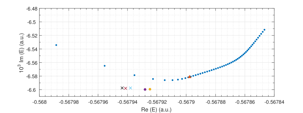
Figure 1: The complex trajectory of $3a_{1}$ MO eigenvalues at $F_{z}=0.1$ a.u. for the CAP method, along with ECS results. The major grid lines on both axes show variation at the $10^{-5}$ level, which illuminates the variation of complex eigenvalues for different solution parameters. The CAP trajectory is marked by blue ${\color[rgb]{0,0,0}\bullet}$, for $\eta\in[0.008,0.06]$. The CAP stabilization method result is shown by the red ${\color[rgb]{0,0,0}\blacktriangle}$. The yellow ${\color[rgb]{0,0,0}\bullet}$ and purple ${\color[rgb]{0,0,0}\bullet}$ are the result of the first and second order CAP corrective schemes. The cyan ${\color[rgb]{0,1,1}\times}$ symbol marks the ECS result with $\xi\approx 1.4$ rad using a coupled differential equations method. The red ${\color[rgb]{0,0,0}\times}$ marks the FEM-ECS with 180 integrator nodes and $\xi=0.5$ rad. The black ${\color[rgb]{0,0,0}\times}$ marks two points, for $\xi=0.5$ and $\xi\approx 1.4$ rad, both with 120 integrator nodes.

Looking at the trajectory and the coalescence of the stabilized value ($n=0$ in the correction scheme) and the perturbatively corrected values at order $n=1,2$ one observes for all the CAP results shown in Fig.  1 agreement at the level of three decimal places.

The ECS method, on the other hand, practically shows no dependence on its scaling parameter $\xi$, but may show some dependence on the accuracy of integration in the FEM-ECS approach. As a note, for the FEM-ECS method we have used 120 integrator nodes for all results given in the tables. We confirmed the accuracy of these results (four decimal places) by an alternative implementation of ECS using a coupled-differential equations approach listed as the cyan ${\color[rgb]{0,1,1}\times}$. We note that the ECS results still have a small issue as far as convergence is concerned, but certainly for the width parameter $\Gamma$ an accurate result has been obtained. The main point to be made is that a direct calculation within the ECS framework yields an answer, and no trajectory computation is required.

Furthermore, in particular consideration of the coupled-differential equation approach for ECS, we can make a further comparison with our FEM-ECS results. For example, for the field strength of $F_{z}=0.08$ a.u., the resonance positions of $1b_{2}$ agree up to four significant digits, and the widths up to three significant digits. The resonance positions of $1b_{1}$ agree up to nine significant digits, and the widths agree up to five significant digits. In other words, the worst agreement still captured the same order of magnitude, along with the first three digits used in scientific notation. Care was taken to make sure that the calculations were similar, but differences in methodology and basis choice (and size) remain as explanations for the disagreements.

III.3 Density plots for the molecular orbitals

We present some graphical results to demonstrate the quality of the partial-wave expanded orbitals which combine an accurate representation for the radial part of the wavefunction with a limited superposition of spherical harmonics to represent the angular portions of the wavefunction. We begin with the MO $3a_{1}$ which is composed of even-$m$ harmonics and the bonding $1b_{2}$ orbital composed of odd-$m$ harmonics: both in the field-free case, and in the cases where the field is aligned (or counter-aligned) with the chosen $z$ axis.

Figure 2: All axes are in atomic units. Contour plots of normalized probability densities for the $3a_{1}$ MO (left column) and the bonding $1b_{2}$ MO (right column), over the molecular plane (denoted $y-z$) with the oxygen nucleus and the protons marked by a white triangle. Top row: field-free case, middle panel: for a field pushing electrons away from oxygen past the protons; bottom panel: opposite field direction. The field strength is $0.1$ a.u. for the case of $3a_{1}$, and $0.2$ a.u. for $1b_{2}$. The contour values (starting from the outside) are $0.005,0.01,0.02$ followed by a regularly spaced sequence of intervals of $0.02$ a.u..

Fig. 2 above shows the probability densities in the molecular plane, labeled as $y-z$. The protons are located at $y\approx\pm 1.428$ and $z\approx 1.096$ atomic units. Looking at the density distributions in the left column we observe how the probability density changes from the field-free case (top row) to a situation in which electrons flow away from oxygen past the protons mostly in the direction along the $z-$axis for one field direction (middle row), and in the opposite direction for the reversed field (bottom row). The calculation for the case with decay was obtained using the CAP method. In the (left) middle panel one can see the relevant orbital for the stabilized eigenvalue value along the trajectory shown in Fig. 1.

For the field in the opposite direction (bottom left panel) the decay rate is smaller by about a factor of four (the magnitude of the imaginary parts is 0.00658 versus 0.00165 atomic units). One can again observe a probability density describing electron flux centered along the $z-$ axis, this time, toward the oxygen atom and beyond. At the same time, an increase in electron density occurs in-between the two protons. One can see for both force orientations along $z$, that the density lobe on the opposite side of the axis (say, the lobe on the positive side of the $z-$axis when the force is in the negative $z$ direction) becomes smaller and has a higher density of contour lines.

For the bonding $1b_{2}$ orbital which is shown for a doubled field strength in the right column ($F_{0,z}=\pm 0.2$ a.u.) a different behavior can be observed. This MO has probability density concentrated between the oxygen and proton nuclei (top right panel). With the field pushing electrons out, away from oxygen, past the protons (middle right panel), one can observe directional flow somewhat along the bond axis with deformed humps in the probability distribution.

For the field pushing in the opposite direction (bottom right panel) emission is favored again in an outward direction. The imaginary parts of the energy eigenvalues have magnitudes of 0.00306 and 0.00169 atomic units respectively for the two cases. This is consistent with what is shown in the probability plots, i.e., a stronger deformation towards larger distances in the middle versus the bottom panel.

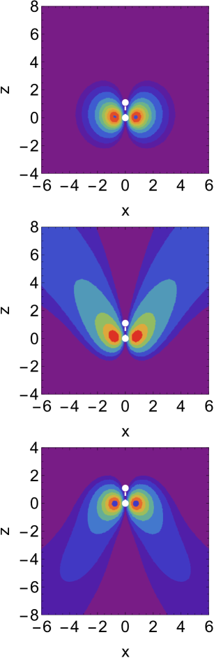
Figure 3: All axes are in atomic units. Contour plots of the normalized probability density for the (highest occupied) $1b_{1}$ MO, over the $x-z$ plane (perpendicular to the molecular plane). White dots mark the oxygen nucleus and the proton location’s projection. Top panel: field-free case, middle panel: for a field with strength $0.2$ a.u. pushing electrons away from oxygen past the protons; bottom panel: opposite field direction. The contour values (starting from the outside) are $0.005,0.01,0.02$ followed by a regularly spaced sequence of intervals of $0.02$ a.u..

In Fig. 3 above the probabilities for the ‘lone’ MO $1b_{1}$ are shown. It is the least bound MO (the so-called highest occupied MO), with probability density concentrated perpendicular to the molecular plane, which in our notation is the $y-z$ plane. Again, we observe an asymmetry for emission when the external force field is aligned or counter-aligned with the $z-$axis. As was done for the $1b_{2}$ MO the field strength was doubled compared to the $3a_{1}$ case to obtain stronger decay rates. The imaginary part magnitudes of the stabilized CAP eigenvalues are approximately 0.0144 and 0.00816 atomic units respectively for the cases shown in the middle vs bottom panel.

To summarize this section we note that the truncation of the partial-wave expansion at $\ell_{\max}=3$ does not prevent us from observing interesting features in the resonance states which describe very distinctive patterns of ionized electron flux. The density plots also display geometrical displacements of the bound parts which are associated with the external field, and these lead to interesting features in the Stark shifts as a function of field orientation and field strengths. Such features were observed recently in HF and CCSD(T) calculations Jagau (2018), but were absent in single-center model potential calculations Laso and Horbatsch (2017).

III.4 Resonance positions and resonance half-widths for molecular orbitals of $\rm H_{2}O$

We now present results for Stark resonance parameters using the FEM-ECS method. In the first subsection the figures are labelled by the molecular orbital (MO) corresponding to the field-free molecule. Note that due to spherical harmonic mixing caused by the DC field, the orbitals obtained for the resonances do not truly correspond to the field-free orbitals. Nevertheless, the progression of the orbital energies is traced by extracting the data from the code which corresponds to a smooth transition of the energies from the field-free molecule to the given field strength. The data is plotted, for the resonance positions (the real parts, or $\mathfrak{Re}~{}\rm(E)$) and half-widths (the negative of the imaginary parts, or $-\mathfrak{Im}~{}\rm(E)$). The half-widths are labelled as $\Gamma/2$, where $\Gamma$ is the decay rate, i.e, the inverse of the decay time constant $\tau$.

To obtain the results of the current work we use a radial box from 0 to 24.3 a.u. with 24 intervals and 11 radial basis functions (polynomial type) per interval. The angular momentum basis is cut at $\ell_{\max}=3$, to include $\ell=0,1,2,3$ and all associated $m$ values. Due to our particular choice of orientation of the water molecule, the $na_{1}$ orbitals have even-$m$ basis functions, while only odd $m$ values contribute for the $1b_{1}$ and $1b_{2}$ orbitals.

For the resonance parameters, the scaling radius is set at 16.2 a.u., and the scaling angle is set at 81 degrees or $\sim$ 1.4 rad, close to the maximum allowed value (90 degrees). The scaling radius is chosen sufficiently large such that the potential energy experienced by the electrons behaves like $-1/r$. The role of the scaling angle $\xi$ is to ensure that at the box boundary (24.3 a.u.) the demand of a vanishing wavefunction does not introduce a significant artefact.

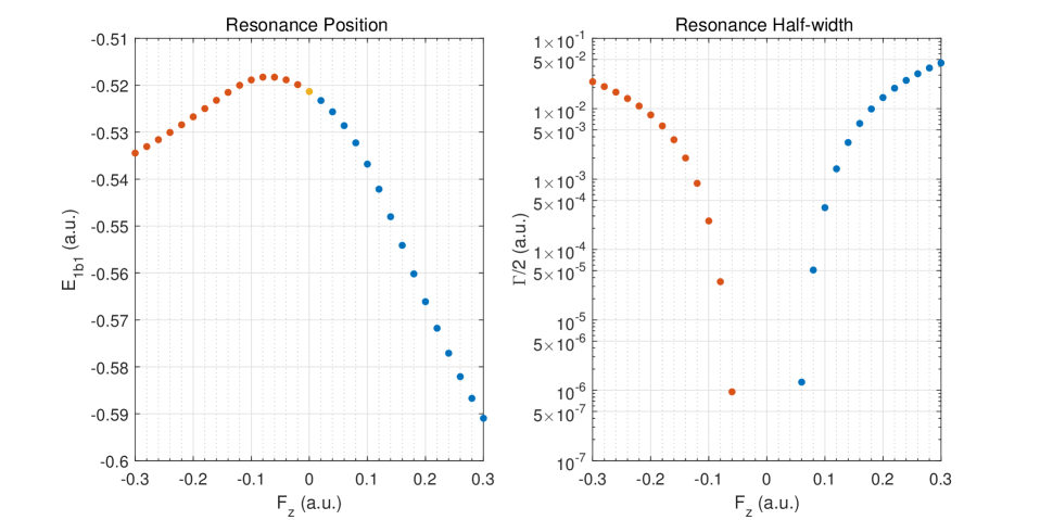
Figure 4: Resonance positions (left panel) and half-widths (right panel) of the $1b_{1}$ valence orbital of $\rm H_{2}O$ in an external DC electric field. The sign of the values of $F_{z}$ (horizontal axis) points in the direction of the force experienced by an electron. The energy position of the free water molecule is given by the yellow marker. The orange markers are for points with the negative values of $F_{z}$ while the blue markers indicate results for $F_{z}>0$. As explained in the text, positive $F_{z}$ values corresponds to the force driving the electrons from the oxygen atom towards the hydrogen atoms and beyond; negative values correspond to the force driving the electrons from the hydrogen atoms towards the oxygen atom and beyond.

In Fig. 4 the results of complex-valued eigenenergies are shown for the outermost valence orbital $1b_{1}$: the left panel shows the energy position of the resonance, and the right panel the negative of the imaginary part, which represents the half-width at half-maximum of the Breit-Wigner resonance. When the electric force is pointing towards the hydrogen atoms, away from the oxygen ($F_{z}>0$), the electrons are pushed outward and towards the protons, thereby lowering their eigenenergy considerably (binding being represented by the magnitude of the real part). When the electric force experienced by the electron is pointing towards the oxygen atom ($F_{z}<0$) the electrons are attracted towards it, causing initially a weak decrease in binding. Eventually the attraction to oxygen increases their binding as the field magnitude increases.

We notice a few remarkable features in these results: first of all, the DC Stark shift is quite asymmetrical about $F_{z}=0$. For negative values, i.e., the external field pushing electron density away from the protons first raises the orbital energy at weak field strength due to the attractive potential, but then the trend turns around as the field strength increases and drives electron density towards the oxygen atom.

This is accompanied by a rise in exponential decay rate as shown in the right panel (orange markers). At weak fields there is the tunneling regime with a very strong dependence of the resonance width on the field strength. As the field strength increases one observes turnover, and approach towards an over-barrier ionization regime.

For the opposite field direction (blue markers), i.e., $F_{z}>0$, a monotonic lowering of the orbital energy is observed. Nevertheless, the decay rate shows a similar growth pattern with field strength, and, in fact, exceeding the rate observed in the opposite direction once the over-barrier regime is reached by about a factor of two.

This orbital has a probability distribution which is perpendicular to the molecular plane formed by the three nuclei. One might therefore assume that the DC shifts are not too strong, and for moderate fields this is indeed the case. Concerning the comparison with a previous model calculation Laso and Horbatsch (2017) which used an effective potential derived from a single-centre HF solution and which was limited to $F_{z}>0$, we observe that the trends are similar. The DC shift is more pronounced in the present calculation, but the behavior of the decay rate is quite comparable.

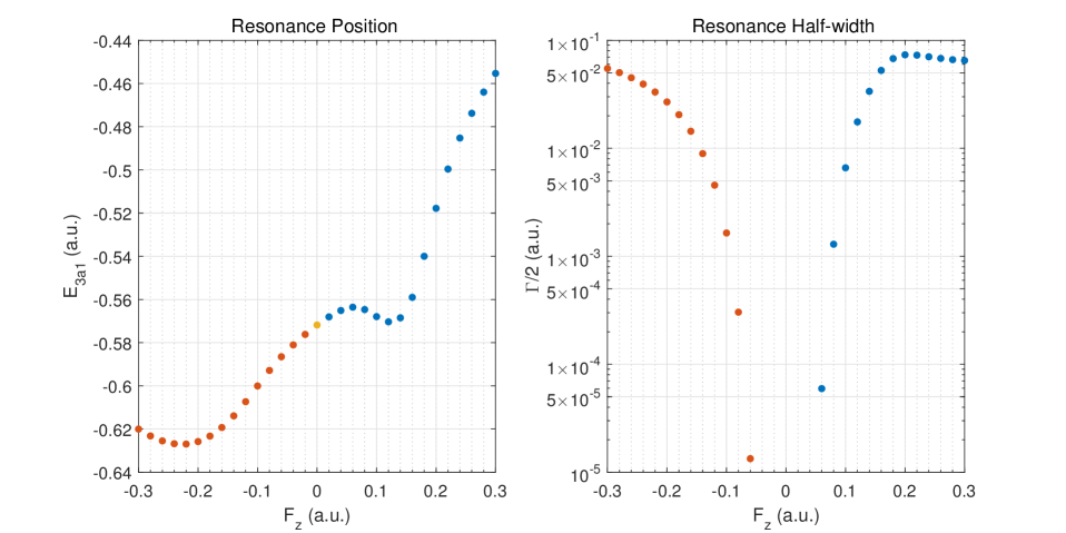
Figure 5: Resonance positions (left panel) and half-widths (right panel) of the $3a_{1}$ valence orbital of water in an external DC electric field.

Fig. 5 shows results for the valence orbital $3a_{1}$ and these are quite remarkable: the resonance position is not changing in a monotonic fashion when the electric force pushes electrons out on the side where the hydrogens are located. The Stark shift becomes in fact very small at some critical field strength. There are two undulating (or wave) features, one on each side of the $F_{z}$ axis. A similar feature was reported by Jagau in their molecular Stark shift results based on the total energy for the $\rm H_{2}O$ molecule Jagau (2018). This is discussed in Sect. III.5.

Comparing these results with the previous work based on the single-center SCF potential with assumed azimuthal symmetry Laso and Horbatsch (2017) indicates that the present work has more geometric flexibility in the resonance solution, and therefore shows more prominent features in the behavior of DC shift and decay rate $\Gamma$ as a function of field strength and field orientation. The work of Ref. Laso and Horbatsch (2017) showed monotonic behavior in the DC shift with a decrease in orbital energy. At small $|F_{z}|$ the widths from these calculations are similar to the current results, but with increasing field strength the decay rate in Ref. Laso and Horbatsch (2017) becomes higher for the case where ionized electrons move away in the direction from oxygen past the two protons by about a factor of two at $|F_{z}|=0.3$ a.u.. Note that the definition of the sign of $F_{z}$ is reversed in the present work with respect to Ref. Laso and Horbatsch (2017) such that it refers to the force experienced by the electron.

To summarize the comparison between the present results and those of Ref. Laso and Horbatsch (2017) we may state that the inclusion of the dependence in the effective potential on the azimuthal angle $\phi$ is important and plays a role in the rich behavior observed for the DC Stark shift of the $3a_{1}$ orbital.

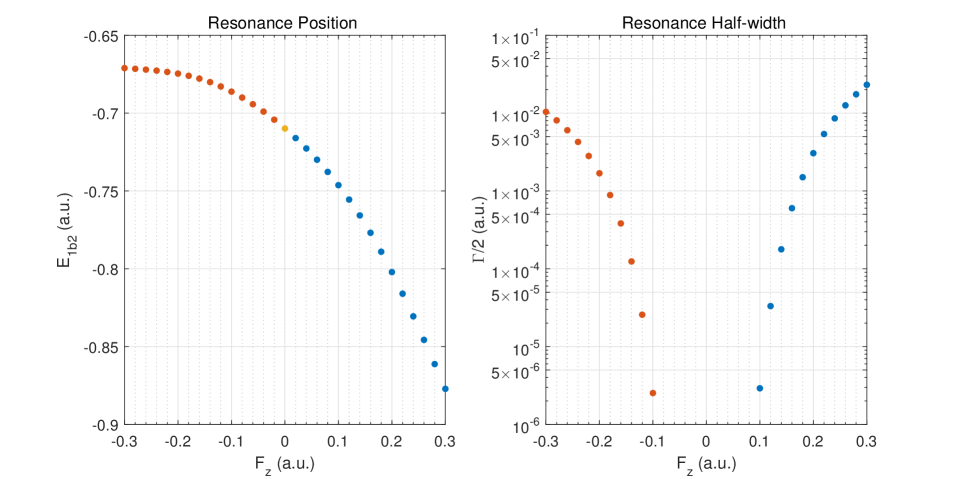
Figure 6: Resonance positions (left panel) and half-widths (right panel) of the $1b_{2}$ valence orbital of water in an external DC electric field.

In Fig. 6 above the results are shown for the bonding orbital $1b_{2}$, which has the strongest binding of the three valence orbitals. We observe that when the electric force points towards the oxygen atom, the electrons actually become slightly less bound, and the opposite is true when the density is pushed towards the protons. Despite the negative Stark shift the ionization rate is stronger for $F_{z}>0$. We also observe that for this deeply bound valence orbital the decay rates are smaller in comparison, and for the given field strength range do not get far beyond the tunneling regime.

We would like to remark on the fact that all three reported orbital calculations were performed independently in a frozen model potential, i.e., no self-consistency based on the orbital densities was attempted. A fully self-consistent calculation, in the sense of DFT, such as, e.g., the OPM approach will cause deviations for the energy shifts and decay rates.

III.5 Comparison with work based on total energy

We now connect our model potential work with the work of Jagau, which is based on the total energy of the molecule, and which was performed at the level of HF theory, as well as a correlated method, namely coupled-cluster theory (CCSD(T)) Jagau (2018). It is an attempt only, because the model potential does not lead to an obvious definition of the total energy.

In HF theory one can express the total energy as

$$E_{\rm HF}=\frac{1}{2}\left(\sum_{j}\epsilon_{j}+\langle\psi_{j}|V_{\rm nuc}|\psi_{j}\rangle\right),$$ (12)

where the sum is over occupied orbitals. The sum of orbital energies may give only one half of the total energy or less, and this is made up by the interaction energy matrix element with the external potential. The reason for the required correction beyond the sum of eigenvalues is that the latter double-count the direct and exchange contributions from the electron-electron repulsion.

In principle, we could calculate such an energy expression, and derive a single decay rate. For now we limit ourselves to a direct sum over orbital energies, which also includes a factor of two to account for the spin degeneracy. A decay rate calculation of this sort corresponds to net ionization, i.e., ten electrons are participating in the decay of the molecule. Of course, this total decay rate is dominated by the contributions from the valence orbitals discussed in Section III.4, but for the DC Stark shift contributions are also coming from the inner orbitals. The prescription for the total (or net) decay rate which is based on the sum of complex-valued orbital energies is consistent with what has been used in the time-dependent domain by employing a straightforward multiplication of orbital probabilities and analyzing a total system survival probability Telnov et al. (2013). The method of Telnov et al. Telnov et al. (2013) results in a sum over orbital decay rates for the net decay rate when applied to our orbitals, due to the multiplication of exponential time-dependencies in the squared probability amplitudes. This is defined by,

$$P_{s}(t)=\prod_{n,\sigma}\int_{0}^{r_{s}}d^{3}r|\Psi_{n,\sigma}(\vec{r},t)|^{2},$$ (13)

where the orbital wavefunctions are given by $\Psi_{n,\sigma}(\vec{r},t)$, along with a decay rate defined as,

$$\Gamma(t)=-\frac{d}{dt}{\rm ln}P_{s}(t).$$ (14)

Fig. 7 shows in the left panel the Stark shift, and in the right panel the full width (decay rate in atomic units). It is compared with the HF and CCSD(T) results, and displays at least a similar pattern. For the Stark shift it appears as if the $1b_{2}$ orbital provides the dominant contribution, as the result is similar in shape. This bonding orbital is relatively deeply bound and the response of the resonance position to the external field is strongest among the valence orbitals as can be seen from the scale in the left panels of Figs. 4 $-$ 6. The Stark shift from the present work based on the sum of orbital energies acquires a strong contribution from the inner $2a_{1}$ orbital, as can be seen in Table 8 in the Appendix, i.e., in Sect. V.3.

The HF results of Ref. Jagau (2018) show a strong turn-around in the Stark shift: as the field strength reaches $F_{z}=-0.15$ a.u. it approaches zero (with CCSD(T) giving a zero crossing at about $F_{z}=-0.13$).

While our results for the MOs $1b_{1}$ and $3a_{1}$ also have a negative shift the $1b_{2}$ and $2a_{1}$ orbitals is responsible for our overall shift not yet showing a complete turn-over. This difference may come from the failure of the sum of eigenvalues properly representing the total energy (cf. Eq. 12). Another explanation could be the use of a frozen target potential in the present work.

For positive values of $F_{z}$ the model potential calculation also exaggerates the shift in comparison to HF theory. Interestingly, adding correlation changes the results by not too much, i.e., CCSD(T) follows the HF shifts at positive values of $F_{z}$, and shows a greater difference in shifts on the other side.

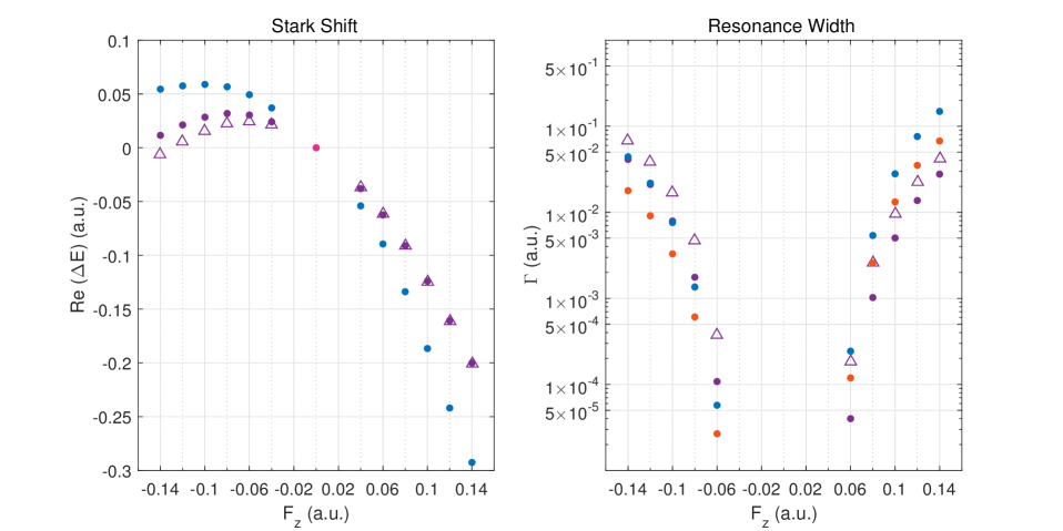
Figure 7: The net resonance positions and widths for Jagau Jagau (2018) and our direct sum method. The blue dots indicate our direct sum method, and the purple dots and triangles indicate the HF and CCSD(T) methods of Jagau Jagau (2018). The red dot in the left panel is the reference by definition; $\Delta E=0$ for $F_{z}=0$. The orange dots on the right panel indicate the widths of the orbital $3a_{1}$.

The net ionization rate in the right panel shows a reasonable comparison between the methods, and for our calculations it is dominated by the $3a_{1}$ orbital contribution (which is shown for comparison without the factor of two for spin degeneracy, i.e., it is the lone orbital width). For $F_{z}>0$ the present net ionization rate is above the HF and CCSD(T) data by a factor of 3-4 at the highest field strengths, since single ionization from the $3a_{1}$ orbital already exceeds those values. For $F_{z}<0$, on the other hand, the present net rate agrees with the HF results at moderate to strong field strengths. Starting at $-0.06$ a.u. moving towards the left, the percentage errors for our net widths with Jagau’s HF values as a reference are $47\%$, $23\%$, $4\%$, $3.7\%$, and $7.3\%$.

One may be concerned with the disagreement between the present results and the HF results at weak to moderate field strengths. In this regime self-consistency effects should be weak, i.e., calculations with frozen versus self-consistent potential ought to give similar results. On the other hand this is the tunneling regime, and it is bound to be very sensitive to details.

The data for the figures are provided in Table 8 in the Appendix (Sect.V.3), which allows one to disentangle the different orbital contributions.

IV Conclusions

We used a model potential for the water molecule developed by the Madrid group Errea et al. (2015), (and used in collaboration with the Toronto group for collision physics), to analyze the molecular properties when exposed to a DC electric field. The calculated DC shifts and decay rates were analyzed both at the molecular orbital level, and at the level of the total energy for net ionization. The former extends previous model work, while the latter allows for comparison with quantum chemistry calculations Jagau (2018).

The computations were performed using an expansion of the molecular orbitals in spherical harmonics. For the current work we included channels up to $\ell_{\max}=3$, and we limited ourselves to only two field directions. Future work should focus on a convergence study (higher values of $\ell_{\max}$), as well as an extension to other field directions for which there will be more mixing between the molecular orbitals, since for the current choice the $na_{1}$ orbitals do not mix with the $1b_{1,2}$ symmetries.

The work has also demonstrated the power of the ECS technique implemented via a finite element method. This technology can be applied now to other small molecules of interest.

Future work should also address to what extent the DC field limit makes predictions which can be carried over to water molecules exposed to intense infrared radiation. This can be handled using the Floquet approach, which was applied to the case of the hydrogen molecular ion in this context Tsogbayar and Horbatsch (2014).

Finally, we would like to encourage the density functional theory community to go beyond the calculation of ground-state systems, and to address the Stark resonance problem. A first important step in this direction would be the extension of the present work to the OPM approach, which should be within reach using an approximation scheme that works well for ground-state systems Engel et al. (2000), and which avoids the need to solve an integral equation for the local potential.

V Appendix

V.1 Details of the matrix elements

Since we implement and discuss the results of the FEM-ECS method, the main computables are the separable matrix elements of the various terms of the Hamiltonian. The oxygen potential, centrifugal potential, and kinetic energy are calculated in a straight-forward manner (however, the kinetic energy is calculated in a symmetric form derived from integration by parts). The main matrix element of concern is the form of the individual hydrogens, which have been expanded. For each hydrogen labelled by $j$,

$$H_{j}^{inlm,i^{\prime}n^{\prime}l^{\prime}m^{\prime}}=4\pi\int drf_{in}(r)f_{i^{\prime}n^{\prime}}(r)\sum_{\lambda=0}^{\lambda_{\max}}\sum_{\mu=-\lambda}^{\lambda}C^{lml^{\prime}m^{\prime}}_{\lambda\mu}\bar{Y}_{\lambda}^{\mu}(\theta^{\prime},\phi_{j})\frac{V_{\lambda}(r)}{2\lambda+1},$$ (15)

where the $f_{in}$ functions are local radial basis functions, $C$ are the results of the spherical parts of the matrix element (Gaunt integrals), the $\bar{Y}_{\lambda}^{\mu}(\theta^{\prime},\phi_{j})$ locate the hydrogens (by their $\theta$ and $\phi$ locations) and the $V_{\lambda}(r)$ are the radial channel dependent parts of the hydrogen potential. Our approach is to calculate the radial part of the matrix element (the integral) using a very fast parallelized 1D integrator that produces a submatrix independent of the spherical basis functions. The sums over $\lambda$ and $\mu$ values are computed after, and the full matrix is produced. The Gaunt integrals are dealt with using Wigner $3j$ coefficients computed beforehand using a code developed by Stone and Wood Stone and Wood (1980). The source code is provided on Wood’s personal web page. This requires a re-write of the above as,

$$H_{j}^{inlm,i^{\prime}n^{\prime}l^{\prime}m^{\prime}}=\sum_{\lambda=0}^{\lambda_{\max}}\sum_{\mu=-\lambda}^{\lambda}\frac{1}{2\lambda+1}C^{lml^{\prime}m^{\prime}}_{\lambda\mu}\bar{Y}_{\lambda}^{\mu}(\theta^{\prime},\phi_{j})\cdot 4\pi\int drf_{in}(r)V_{\lambda}(r)f_{i^{\prime}n^{\prime}}(r).$$ (16)

Perhaps more clearly, a submatrix of lower structure denoted by $a$ and $b$ indices which correspond to $f_{in}$ and $f_{i^{\prime}n^{\prime}}$ is formed, then combined with the angular basis functions by considering a higher structure denoted by $c$ and $d$ indices corresponding $lm$ and $l^{\prime}m^{\prime}$. Each $lm/l^{\prime}m^{\prime}$ block of the higher structure contains every part of the lower structure. The full matrix is of course 2D, denoted by $\alpha$ and $\beta$ indices, but contains 4 dimensions of structure.

The full matrix for this problem that then looks like

$$H_{\alpha\beta}=\left(\begin{tabular}[]{c c c c}$H^{0000}$&$H^{001-1}$&$H^{0010}$&\ldots\\ $H^{1-100}$&$H^{1-11-1}$&$H^{1-110}$&\ldots\\ $H^{1000}$&$H^{101-1}$&$H^{1010}$&\ldots\\ \vdots&\vdots&\vdots&$\ddots$\\ \end{tabular}\right),$$ (17)

where $H^{lml^{\prime}m^{\prime}}$ is a submatrix where $l,m,l^{\prime}m^{\prime}$ are fixed and $i,n,i^{\prime},n^{\prime}$ are not.

The submatrices at low order have a radial part that looks like,

$$H_{k}=\left(\begin{tabular}[]{c c c c c}$\langle f_{11}|H_{k}|f_{11}\rangle$&$\langle f_{11}|H_{k}|f_{13}\rangle$&$\langle f_{11}|H_{k}|f_{12}\rangle$&$0$&$0$\\ $\langle f_{13}|H_{k}|f_{11}\rangle$&$\langle f_{13}|H_{k}|f_{13}\rangle$&$\langle f_{13}|H_{k}|f_{12}\rangle$&$0$&$0$\\ $\langle f_{12}|H_{k}|f_{11}\rangle$&$\langle f_{12}|H_{k}|f_{13}\rangle$&$\langle f_{12}|H_{k}|f_{12}\rangle+\langle f_{21}|H_{k}|f_{21}\rangle$&$\langle f_{21}|H_{k}|f_{23}\rangle$&$\langle f_{21}|H_{k}|f_{22}\rangle$\\ $0$&$0$&$\langle f_{23}|H_{k}|f_{21}\rangle$&$\langle f_{23}|H_{k}|f_{23}\rangle$&$\langle f_{23}|H_{k}|f_{22}\rangle$\\ $0$&$0$&$\langle f_{22}|H_{k}|f_{21}\rangle$&$\langle f_{22}|H_{k}|f_{23}\rangle$&$\langle f_{22}|H_{k}|f_{22}\rangle$\\ \end{tabular}\right).$$ (18)

The overlap between the two blocks denotes a continuity condition at the boundary between the two radial intervals (denoted by the two blocks). The letter $k$ denotes the appropriate radial Hamiltonian term, two of which are the $V_{\lambda}(r)$. The others are the centrifugal potential, the oxygen potential, and the kinetic energy. Each of these radial matrices is combined with the appropriate angular terms which involve Gaunt integrals. Thus $H^{lml^{\prime}m^{\prime}}$ is really an element by element sum over submatrices that look like this, or $H^{lml^{\prime}m^{\prime}}=\sum_{k}A_{k}^{lml^{\prime}m^{\prime}}H_{k}$, where $A_{k}^{lml^{\prime}m^{\prime}}$ is the appropriate angular piece. For the hydrogens $A_{k}^{lml^{\prime}m^{\prime}}$ contains the double sum in Eq. (15). The sum denoted by the capital sigma denotes the sum over every Hamiltonian term listed by $k$. $A_{k}^{lml^{\prime}m^{\prime}}$ is basically just the spherical harmonic overlap matrix element for all other Hamiltonian terms save for the DC potential, which contains a third spherical harmonic, i.e., $\rm\cos(\theta)$.

Two caveats of using Wigner coefficients arise. The first is that not all spherical integrals involve three spherical harmonics (specifically those involving Hamiltonian terms which lack spherical dependence). This is of course solved by using the $l=0$ spherical harmonic as the middle term in the integral (where the left and right terms are the spherical basis functions). However, this spherical harmonic is a constant, so the Wigner result must be multiplied by the inverse of the constant. A similar constant is required for the $\rm cos(\theta)$ term in the DC potential. The second caveat is that the Wigner coefficients are defined without a bar or star on the left spherical harmonic. Therefore, the appropriate response to the barring process in forming the matrix element is to multiply the $m$ quantum number of the left spherical harmonic in the Wigner coefficient by $-1$, and to multiply the entire result by $(-1)^{m}$, where the $m$ value corresponds to the unbarred spherical harmonic value. This arises from the standard definition used for spherical harmonics, $\bar{Y}_{l}^{m}=(-1)^{m}Y_{l}^{-m}$.

V.2 Resonance positions and resonance half-widths (tables)

Below, $-\mathfrak{Im}=\Gamma/2$, or half the resonance width. Numbers with less than 4 significant digits have trailing zeroes. This number of sig. digs. was chosen in accord with the agreement for the real part of the energy between ECS/CAP for the orbital/field strength in Fig. 1. This applies for the real part $\mathfrak{Re}$ in the data below. In the same figure the imaginary part shows agreement for 4 decimal places with non-scientific notation (not 4 sig. digs. per the tables). The small imaginary numbers (below $10^{-7}$) should be trusted to fewer digits.

V.2.1 Positive force values

MO: $1b_{1}$
$\rm F_{z}$	$\mathfrak{Re}$	$\mathfrak{Im}~{}$
0.02	$-0.523\,258\,902\,779\,067\,28$	NA
0.04	$-0.525\,659\,266\,074\,847\,36$	$-4.953\,812\,982\,788\,332\,9\text{\times}{10}^{-010}$
0.06	$-0.528\,611\,147\,010\,421\,67$	$-1.306\,869\,996\,448\,888\,6\text{\times}{10}^{-006}$
0.08	$-0.532\,268\,622\,083\,351\,46$	$-5.110\,458\,190\,864\,888\,2\text{\times}{10}^{-005}$
0.10	$-0.536\,801\,517\,285\,124\,93$	$-3.929\,659\,946\,946\,665\,3\text{\times}{10}^{-004}$
0.12	$-0.542\,145\,344\,460\,908\,90$	$-1.399\,926\,051\,878\,737\,3\text{\times}{10}^{-003}$
0.14	$-0.548\,018\,782\,402\,080\,35$	$-3.312\,652\,955\,375\,724\,4\text{\times}{10}^{-003}$
0.16	$-0.554\,115\,812\,271\,271\,27$	$-6.169\,010\,963\,255\,118\,0\text{\times}{10}^{-003}$
0.18	$-0.560\,199\,010\,726\,856\,41$	$-9.907\,925\,448\,753\,801\,2\text{\times}{10}^{-003}$
0.20	$-0.566\,115\,593\,011\,398\,35$	$-1.440\,286\,339\,008\,452\,4\text{\times}{10}^{-002}$
0.22	$-0.571\,772\,961\,428\,758\,22$	$-1.955\,806\,371\,709\,560\,9\text{\times}{10}^{-002}$
0.24	$-0.577\,098\,592\,196\,298\,11$	$-2.524\,560\,047\,798\,258\,1\text{\times}{10}^{-002}$
0.26	$-0.582\,093\,946\,551\,329\,51$	$-3.137\,944\,566\,716\,547\,5\text{\times}{10}^{-002}$
0.28	$-0.586\,712\,099\,842\,390\,92$	$-3.789\,907\,066\,516\,620\,7\text{\times}{10}^{-002}$
0.30	$-0.590\,955\,304\,123\,339\,30$	$-4.468\,985\,426\,814\,211\,4\text{\times}{10}^{-002}$

Table 2: Resonance positions and half-widths for the molecular orbital $1b_{1}$ of $\rm H_{2}O$ as a function of $F_{z}>0$. $\mathfrak{Re}$ refers to the real part of the energy, and $\mathfrak{Im}$ refers to the imaginary part of the energy.

MO: $3a_{1}$
$\rm F_{z}$	$\mathfrak{Re}$	$\mathfrak{Im}~{}$
0.02	$-0.568\,061\,799\,412\,733\,16$	$-1.436\,302\,865\,864\,240\,2\text{\times}{10}^{-012}$
0.04	$-0.565\,114\,302\,846\,303\,82$	$-6.473\,652\,679\,725\,726\,2\text{\times}{10}^{-008}$
0.06	$-0.563\,578\,936\,581\,746\,07$	$-5.949\,226\,340\,790\,840\,6\text{\times}{10}^{-005}$
0.08	$-0.564\,677\,418\,998\,582\,81$	$-1.292\,783\,194\,874\,606\,1\text{\times}{10}^{-003}$
0.10	$-0.567\,943\,620\,494\,643\,97$	$-6.597\,767\,243\,757\,410\,1\text{\times}{10}^{-003}$
0.12	$-0.570\,353\,888\,104\,330\,52$	$-1.755\,712\,123\,462\,472\,4\text{\times}{10}^{-002}$
0.14	$-0.568\,505\,045\,066\,041\,60$	$-3.369\,005\,113\,945\,239\,3\text{\times}{10}^{-002}$
0.16	$-0.559\,014\,417\,078\,722\,68$	$-5.263\,528\,917\,193\,777\,8\text{\times}{10}^{-002}$
0.18	$-0.540\,005\,585\,625\,496\,17$	$-6.779\,542\,151\,000\,038\,4\text{\times}{10}^{-002}$
0.20	$-0.517\,793\,223\,438\,974\,71$	$-7.344\,465\,641\,171\,879\,5\text{\times}{10}^{-002}$
0.22	$-0.499\,616\,853\,691\,222\,22$	$-7.286\,255\,018\,245\,563\,2\text{\times}{10}^{-002}$
0.24	$-0.485\,241\,484\,565\,202\,11$	$-7.044\,196\,725\,102\,781\,8\text{\times}{10}^{-002}$
0.26	$-0.473\,785\,981\,889\,265\,30$	$-6.804\,440\,188\,656\,509\,0\text{\times}{10}^{-002}$
0.28	$-0.463\,966\,802\,315\,897\,04$	$-6.621\,592\,479\,629\,080\,7\text{\times}{10}^{-002}$
0.30	$-0.455\,315\,891\,289\,878\,04$	$-6.505\,479\,908\,461\,360\,4\text{\times}{10}^{-002}$

Table 3: Resonance positions and half-widths for the molecular orbital $3a_{1}$ of $\rm H_{2}O$ as a function of $F_{z}>0$. $\mathfrak{Re}$ refers to the real part of the energy, and $\mathfrak{Im}$ refers to the imaginary part of the energy.

MO: $1b_{2}$
$\rm F_{z}$	$\mathfrak{Re}$	$\mathfrak{Im}~{}$
0.02	$-0.716\,047\,097\,363\,987\,53$	$-3.066\,876\,801\,277\,829\,0\text{\times}{10}^{-012}$
0.04	$-0.722\,722\,673\,637\,223\,98$	$-4.746\,929\,281\,354\,368\,6\text{\times}{10}^{-012}$
0.06	$-0.729\,951\,776\,640\,439\,86$	$-9.459\,405\,008\,836\,352\,2\text{\times}{10}^{-011}$
0.08	$-0.737\,782\,042\,002\,557\,59$	$-6.664\,333\,717\,714\,452\,8\text{\times}{10}^{-008}$
0.10	$-0.746\,282\,629\,338\,975\,93$	$-2.907\,848\,865\,712\,229\,0\text{\times}{10}^{-006}$
0.12	$-0.755\,557\,648\,978\,429\,03$	$-3.311\,987\,352\,094\,070\,6\text{\times}{10}^{-005}$
0.14	$-0.765\,732\,552\,860\,719\,28$	$-1.777\,275\,343\,150\,554\,2\text{\times}{10}^{-004}$
0.16	$-0.776\,897\,959\,929\,042\,54$	$-5.999\,952\,700\,855\,735\,7\text{\times}{10}^{-004}$
0.18	$-0.789\,061\,353\,347\,486\,73$	$-1.500\,423\,012\,412\,869\,6\text{\times}{10}^{-003}$
0.20	$-0.802\,148\,886\,955\,225\,02$	$-3.053\,989\,055\,880\,852\,0\text{\times}{10}^{-003}$
0.22	$-0.816\,039\,032\,928\,456\,92$	$-5.386\,079\,752\,058\,307\,3\text{\times}{10}^{-003}$
0.24	$-0.830\,595\,289\,311\,469\,31$	$-8.554\,380\,881\,524\,850\,0\text{\times}{10}^{-003}$
0.26	$-0.845\,704\,031\,883\,568\,02$	$-1.257\,921\,591\,013\,899\,0\text{\times}{10}^{-002}$
0.28	$-0.861\,253\,993\,782\,173\,60$	$-1.745\,312\,881\,695\,081\,1\text{\times}{10}^{-002}$
0.30	$-0.877\,169\,015\,413\,208\,57$	$-2.313\,173\,712\,650\,225\,3\text{\times}{10}^{-002}$

Table 4: Resonance positions and half-widths for the molecular orbital $1b_{2}$ of $\rm H_{2}O$ as a function of $F_{z}>0$. $\mathfrak{Re}$ refers to the real part of the energy, and $\mathfrak{Im}$ refers to the imaginary part of the energy.

V.2.2 Negative force values

MO: $~{}1b_{1}$
$\rm F_{z}$	$\mathfrak{Re}$	$\mathfrak{Im}$
-0.02	$-0.519\,871\,458\,738\,885\,29$	$-2.769\,168\,223\,061\,699\,9\text{\times}{10}^{-012}$
-0.04	$-0.518\,845\,921\,072\,488\,72$	$-3.940\,287\,865\,900\,112\,8\text{\times}{10}^{-010}$
-0.06	$-0.518\,285\,696\,764\,693\,72$	$-9.511\,445\,048\,758\,549\,0\text{\times}{10}^{-007}$
-0.08	$-0.518\,267\,265\,141\,535\,76$	$-3.488\,930\,279\,861\,830\,3\text{\times}{10}^{-005}$
-0.10	$-0.518\,866\,690\,630\,337\,86$	$-2.546\,307\,895\,036\,838\,8\text{\times}{10}^{-004}$
-0.12	$-0.520\,012\,204\,291\,138\,15$	$-8.711\,123\,591\,947\,513\,7\text{\times}{10}^{-004}$
-0.14	$-0.521\,521\,092\,603\,463\,58$	$-1.993\,753\,921\,281\,262\,7\text{\times}{10}^{-003}$
-0.16	$-0.523\,215\,278\,280\,644\,62$	$-3.623\,001\,222\,305\,001\,5\text{\times}{10}^{-003}$
-0.18	$-0.524\,976\,918\,133\,451\,04$	$-5.698\,978\,147\,160\,807\,4\text{\times}{10}^{-003}$
-0.20	$-0.526\,725\,611\,173\,077\,04$	$-8.156\,613\,521\,036\,814\,4\text{\times}{10}^{-003}$
-0.22	$-0.528\,426\,805\,501\,874\,04$	$-1.092\,231\,396\,297\,758\,9\text{\times}{10}^{-002}$
-0.24	$-0.530\,057\,307\,903\,604\,50$	$-1.395\,344\,730\,852\,617\,8\text{\times}{10}^{-002}$
-0.26	$-0.531\,601\,859\,494\,371\,33$	$-1.719\,193\,939\,192\,310\,8\text{\times}{10}^{-002}$
-0.28	$-0.533\,073\,244\,432\,088\,37$	$-2.060\,757\,968\,767\,325\,9\text{\times}{10}^{-002}$
-0.30	$-0.534\,457\,591\,063\,385\,53$	$-2.418\,036\,150\,456\,433\,9\text{\times}{10}^{-002}$

Table 5: Resonance positions and half-widths for the molecular orbital $1b_{1}$ of $\rm H_{2}O$ as a function of $F_{z}<0$. $\mathfrak{Re}$ refers to the real part of the energy, and $\mathfrak{Im}$ refers to the imaginary part of the energy.

MO: $~{}3a_{1}$
$\rm F_{z}$	$\mathfrak{Re}$	$\mathfrak{Im}$
-0.02	$-0.576\,180\,812\,025\,483\,99$	$-2.492\,189\,162\,034\,544\,1\text{\times}{10}^{-013}$
-0.04	$-0.581\,054\,667\,942\,546\,12$	$-1.437\,050\,912\,214\,196\,3\text{\times}{10}^{-008}$
-0.06	$-0.586\,522\,490\,212\,879\,06$	$-1.335\,267\,946\,472\,648\,4\text{\times}{10}^{-005}$
-0.08	$-0.592\,872\,622\,381\,148\,35$	$-3.037\,359\,643\,069\,876\,9\text{\times}{10}^{-004}$
-0.10	$-0.600\,058\,183\,622\,098\,51$	$-1.642\,920\,502\,662\,374\,6\text{\times}{10}^{-003}$
-0.12	$-0.607\,334\,579\,266\,311\,62$	$-4.553\,504\,587\,980\,222\,6\text{\times}{10}^{-003}$
-0.14	$-0.613\,904\,338\,431\,062\,29$	$-8.928\,131\,929\,705\,773\,0\text{\times}{10}^{-003}$
-0.16	$-0.619\,288\,773\,694\,880\,89$	$-1.438\,722\,788\,298\,935\,9\text{\times}{10}^{-002}$
-0.18	$-0.623\,281\,124\,102\,496\,14$	$-2.048\,111\,796\,181\,285\,2\text{\times}{10}^{-002}$
-0.20	$-0.625\,810\,017\,416\,997\,49$	$-2.687\,101\,222\,592\,584\,0\text{\times}{10}^{-002}$
-0.22	$-0.626\,959\,854\,511\,987\,32$	$-3.321\,789\,592\,969\,069\,7\text{\times}{10}^{-002}$
-0.24	$-0.626\,799\,221\,371\,713\,62$	$-3.934\,843\,622\,151\,568\,1\text{\times}{10}^{-002}$
-0.26	$-0.625\,495\,148\,543\,637\,75$	$-4.502\,754\,453\,783\,502\,2\text{\times}{10}^{-002}$
-0.28	$-0.623\,200\,598\,891\,373\,58$	$-5.023\,412\,331\,466\,534\,1\text{\times}{10}^{-002}$
-0.30	$-0.620\,026\,937\,906\,609\,57$	$-5.483\,129\,390\,020\,530\,9\text{\times}{10}^{-002}$

Table 6: Resonance positions and half-widths for the molecular orbital $3a_{1}$ of $\rm H_{2}O$ as a function of $F_{z}<0$. $\mathfrak{Re}$ refers to the real part of the energy, and $\mathfrak{Im}$ refers to the imaginary part of the energy.

MO: $~{}1b_{2}$
$\rm F_{z}$	$\mathfrak{Re}$	$\mathfrak{Im}$
-0.02	$-0.704\,223\,921\,051\,313\,59$	$NA$
-0.04	$-0.699\,030\,416\,860\,898\,73$	$-4.353\,185\,931\,177\,177\,6\text{\times}{10}^{-012}$
-0.06	$-0.694\,296\,942\,863\,761\,76$	$-1.116\,465\,866\,022\,828\,7\text{\times}{10}^{-010}$
-0.08	$-0.690\,019\,617\,211\,700\,91$	$-6.553\,903\,238\,477\,129\,3\text{\times}{10}^{-008}$
-0.10	$-0.686\,207\,904\,581\,939\,25$	$-2.526\,688\,740\,121\,961\,4\text{\times}{10}^{-006}$
-0.12	$-0.682\,889\,547\,514\,860\,97$	$-2.566\,869\,428\,407\,542\,4\text{\times}{10}^{-005}$
-0.14	$-0.680\,094\,209\,602\,702\,06$	$-1.240\,335\,135\,492\,944\,9\text{\times}{10}^{-004}$
-0.16	$-0.677\,820\,071\,234\,687\,35$	$-3.822\,355\,963\,377\,553\,0\text{\times}{10}^{-004}$
-0.18	$-0.676\,021\,550\,562\,675\,43$	$-8.841\,699\,753\,186\,362\,6\text{\times}{10}^{-004}$
-0.20	$-0.674\,623\,684\,461\,673\,20$	$-1.685\,584\,454\,028\,334\,2\text{\times}{10}^{-003}$
-0.22	$-0.673\,544\,191\,713\,923\,10$	$-2.813\,240\,398\,062\,715\,9\text{\times}{10}^{-003}$
-0.24	$-0.672\,706\,789\,404\,238\,11$	$-4.264\,193\,910\,148\,947\,9\text{\times}{10}^{-003}$
-0.26	$-0.672\,051\,621\,959\,890\,99$	$-6.025\,325\,109\,371\,032\,0\text{\times}{10}^{-003}$
-0.28	$-0.671\,525\,284\,414\,282\,16$	$-8.071\,486\,800\,402\,238\,5\text{\times}{10}^{-003}$
-0.30	$-0.671\,095\,985\,811\,888\,23$	$-1.037\,347\,688\,898\,384\,6\text{\times}{10}^{-002}$

Table 7: Resonance positions and half-widths for the molecular orbital $1b_{2}$ of $\rm H_{2}O$ as a function of $F_{z}<0$. $\mathfrak{Re}$ refers to the real part of the energy, and $\mathfrak{Im}$ refers to the imaginary part of the energy.

V.3 Comparison with HF total ionization rates

Table 8 contains the Stark shifts and widths of relevant orbitals, and total Stark shifts and resonance widths, to be compared with with the HF results of Jagau Jagau (2018). We carry out a direct sum (written $\rm DS~{}(2)$ for a sum of all orbitals, where the two indicates double occupation due to spin degeneracy) of occupied orbitals to find the net energy and shifts. The bottom two orbitals ($1a_{1}$ and $2a_{1}$) are left out when their values are too small to be comparable to the net HF values, which only happens for the widths and not the Stark shifts. The HF row references Jagau Jagau (2018).

		$\mathfrak{Re}~{}\Delta\rm E$
$F_{z}$		0.04	0.06	0.08	0.10	0.12	0.14
$1a_{1}$		$-0.000013$	$-0.000021$	$-0.000028$	$-0.000037$	$-0.000045$	$-0.000055$
$2a_{1}$		$-0.016565$	$-0.025636$	$-0.035222$	$-0.045316$	$-0.055919$	$-0.067036$
$1b_{2}$		$-0.012833$	$-0.020062$	$-0.027892$	$-0.036393$	$-0.045668$	$-0.055843$
$3a_{1}$		$0.006711$	$0.008246$	$0.007148$	$0.003881$	$0.001471$	$0.003320$
$1b_{1}$		$-0.004319$	$-0.007271$	$-0.010928$	$-0.015461$	$-0.020805$	$-0.026680$
$\rm DS$ (2)		$-0.054039$	$-0.089488$	$-0.133846$	$-0.186651$	$-0.241933$	$-0.292585$
HF		$-0.038045$	$-0.062476$	$-0.091129$	$-0.124048$	$-0.160648$	$-0.200088$
		$\Gamma$
$F_{z}$		0.04	0.06	0.08	0.10	0.12	0.14
$1b_{2}$		0.000000	0.000000	0.000000	0.000006	0.000066	0.000355
$3a_{1}$		0.000000	0.000119	0.002586	0.013196	0.035114	0.067380
$1b_{1}$		0.000000	0.000003	0.000102	0.000786	0.002800	0.006625
$\rm DS~{}(2)$		0.000000	0.000243	0.005376	0.027975	0.075961	0.148723
HF		0.000000	0.000040	0.001021	0.005029	0.013694	0.027745
		$\mathfrak{Re}~{}\Delta\rm E$
$F_{z}$		$-0.04$	$-0.06$	$-0.08$	$-0.10$	$-0.12$	$-0.14$
$1a_{1}$		0.000011	0.000016	0.000020	0.000024	0.000028	0.000031
$2a_{1}$		0.014373	0.020694	0.026410	0.031497	0.035926	0.039666
$1b_{2}$		0.010859	0.015593	0.019870	0.023682	0.027000	0.029797
$3a_{1}$		$-0.009230$	$-0.014697$	$-0.021048$	$-0.028233$	$-0.035510$	$-0.042079$
$1b_{1}$		0.002494	0.003054	0.003073	0.002473	0.001328	$-0.000181$
$\rm DS$ (2)		0.037016	0.049319	0.056651	0.058886	0.057544	0.054463
HF		0.024155	0.030418	0.031849	0.028404	0.021187	0.011549
		$\Gamma$
$F_{z}$		$-0.04$	$-0.06$	$-0.08$	$-0.10$	$-0.12$	$-0.14$
$1b_{2}$		0.000000	0.000000	0.000000	0.000005	0.000051	0.000248
$3a_{1}$		0.000000	0.000027	0.000607	0.003286	0.009107	0.017856
$1b_{1}$		0.000000	0.000002	0.000070	0.000509	0.001742	0.003988
$\rm DS~{}(2)$		0.000000	0.000057	0.001355	0.007600	0.021801	0.044185
HF		0.000006	0.000108	0.001759	0.007911	0.021029	0.041178

Table 8: Stark shifts and widths for the valence orbitals of the water molecule for different force strengths, along with the total molecular Stark shifts and widths under DS (2). All results are from the current work except for HF which references Jagau Jagau (2018).