Dirac States in an Inclined Two-Dimensional Su-Schrieffer-Heeger Model

Abstract

We propose to realize Dirac states in an inclined two-dimensional Su-Schrieffer-Heeger model on a square lattice. We show that a pair of Dirac points protected by space-time inversion symmetry appear in the semimetal phase. The locations of these Dirac points are not pinned to any high-symmetry points of the Brillouin zone but are tunable through parameter modulations. Interestingly, the merging of two Dirac points undergoes a topological phase transition that leads to either a weak topological insulator or a nodal-line semimetal. We provide a systematic analysis of these topological phases from both bulk and boundary perspectives combined with symmetry arguments. We also discuss feasible experimental platforms to realize our model.

I Introduction

Two-dimensional (2D) massless Dirac states have attracted tremendous attention in condensed matter physics and material science since the successful realization of graphene Novoselov et al. (2005); Castro Neto et al. (2009); Liu et al. (2011); Malko et al. (2012); Young and Kane (2015). Dirac states in graphene exhibit particular transport properties such as anomalous quantum Hall effect Zhang et al. (2005), minimum conductivity Ando et al. (2002); Tworzydło et al. (2006), and Klein tunneling Katsnelson et al. (2006); Stander et al. (2009). Dirac points in graphene are pinned to the corners of the hexagonal Brillouin zone (BZ) by $C_{3v}$ group symmetry of the honeycomb lattice. They can only be slightly shifted by applying external strain Pereira et al. (2009). As the large momentum separation of the Dirac point ensures the well-defined valley degrees of freedom, graphene provides many interesting applications such as valley filters Rycerz et al. (2007) and valleytronics Xiao et al. (2007); Yao et al. (2008).

If we are able to manipulate Dirac cones, such as their locations and shape, we may change the properties of the system significantly. For instance, the merging of two Dirac points can transform the system from a semimetal to a trivial insulator Montambaux et al. (2009); Feilhauer et al. (2015) and deformed Dirac cones show anisotropic transport Pereira et al. (2009). Therefore, searching for alternative 2D platforms that host Dirac states with conveniently tunable properties, such as the synthetic honeycomb lattice Feilhauer et al. (2015); Wunsch et al. (2008); Tarruell et al. (2012); Bellec et al. (2013); Real et al. (2020), is of fundamental interest.

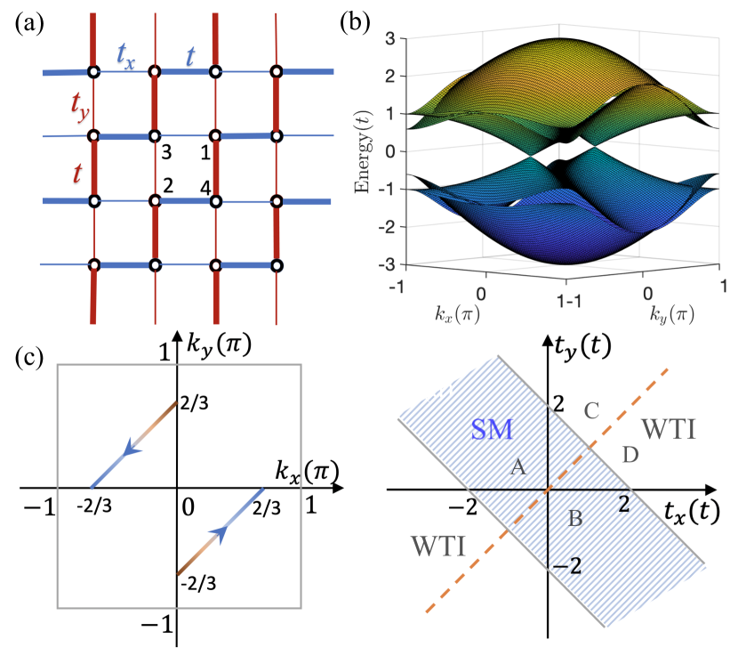
Figure 1: (a) Schematic of the inclined 2D SSH lattice. Blue (red) thick and thin bonds mark alternately dimerized hopping strengths in $x(y)$-direction. (b) Band structure of the inclined 2D SSH model with a pair of Dirac points. Here, we take $t_{x}=0.2t$ and $t_{y}=0.8t$. (c) Moving pattern of the pair of Dirac points corresponding to the condition in Eq. (5). (d) Phase diagram of the inclined 2D SSH model in the $(t_{x},t_{y})$ parameter space. The shadowed region (excluding the orange dashed line) represents the semimetal (SM) with a pair of Dirac points. The orange dashed line at $t_{x}=t_{y}$ corresponds to the nodal-line semimetal. Other regions denote the weak topological insulator (WTI) regime. The four points $A,B,C$, and $D$ label the representative phase points that we refer to in the text.

In this work, we propose to realize 2D Dirac states with tunable properties on a Su-Schrieffer-Heeger (SSH) square lattice. Recently, research activities related to the generalization of the SSH model Su et al. (1979) to 2D have attracted broad interest Liu and Wakabayashi (2017); Benalcazar et al. (2017a, b) and sparked the fast-expanding field of higher-order topological insulators Song et al. (2017); Schindler et al. (2018a, b); Imhof et al. (2018); Serra-Garcia et al. (2018); Xie et al. (2019); Chen et al. (2019); Peterson et al. (2018); Li et al. (2018); Jeon et al. (2022); Zhang et al. (2020); Li et al. (2020); Wei et al. (2021); Li and Wu (2020); Zhang and Trauzettel (2020); Li et al. (2021a). In our proposal, we consider an inclined 2D SSH model with alternately dimerized patterns [Fig. 1(a)]. Different from previous 2D SSH models Liu and Wakabayashi (2017); Benalcazar et al. (2017a, b), such an inclined 2D SSH model hosts massless Dirac states in the BZ within a broad parameter range [Figs. 1(b,d)]. We show that the Dirac points are protected by a space-time inversion symmetry. Moreover, we find that the locations of Dirac points are highly tunable by hopping parameters [Fig. 1(c)]. In contrast to artificial graphene, the merging of two Dirac points in our model experiences a particular topological phase transition resulting in topological phases, i.e., such as weak topological insulator or nodal-line semimetal [Fig. 1(d)]. We demonstrate the topological origin of these phases by employing topological invariants, boundary signatures, and symmetry arguments. We also discuss how to realize our model experimentally based on synthetic quantum materials.

The remainder of this paper is organized as follows. Section II introduces the inclined 2D SSH model. Section III presents the tunable Dirac states on the inclined 2D SSH model. Section IV discusses symmetry protection on these Dirac states. Section V considers the topological phase transition induced by merging of Dirac points. Section VI exhibits the special anisotropic projection properties of Dirac states in our model. Section VII concludes our results with a discussion. Technical details are discussed in four appendices.

II Inclined two-dimensional Su-Schrieffer-Heeger model

We consider a particular 2D SSH model, as shown in Fig. 1(a), where the weak (thin) bonds and strong (thick) bonds are alternately dimerized along the two adjacent parallel lattice rows ($x$-direction) or columns ($y$-direction). We call it the inclined 2D SSH model. There are four orbital degrees of freedom in each unit cell (labeled as $1-4$). We consider spinless fermions, for clarity. The effective Bloch Hamiltonian describing the inclined 2D SSH model in reciprocal space reads

$$H({\bf k})=\left(\begin{array}[]{cc}0&q({\bf k})\\ q^{\dagger}({\bf k})&0\end{array}\right),$$ (1)

$$q({\bf k})\equiv\left(\begin{array}[]{cc}t_{x}+te^{ik_{x}}&t+t_{y}e^{ik_{y}}\\ t_{y}+te^{-ik_{y}}&t+t_{x}e^{-ik_{x}}\end{array}\right),$$ (2)

where ${\bf k}=(k_{x},k_{y})$ is the 2D wave-vector; $t$ and $t_{x/y}$ are the staggered hopping amplitudes along $x/y$-directions. Without loss of generality, we set the lattice constant to be unity and assume $t>0$ hereafter. The basis is $(\Psi_{{\bf k}1},\Psi_{{\bf k}2},\Psi_{{\bf k}3},\Psi_{{\bf k}4})$ of Bloch states constructed on the four sites of the unit cell. The Hamiltonian in Eq. (1) respects chiral (sublattice) symmetry, as indicated by its block off-diagonal form. Explicitly, chiral symmetry yields $\mathcal{C}H({\bf k})\mathcal{C}^{-1}=-H({\bf k})$ with chiral-symmetry operator $\mathcal{C}=\tau_{3}\otimes\sigma_{0}$, where $\tau$ and $\sigma$ are Pauli matrices for different orbital degrees of freedom in the unit cell. The energy bands of Eq. (1) are obtained as

$$E_{\eta}^{\pm}({\bf k})=\pm\sqrt{\xi_{\eta}^{2}({\bf k})+\zeta_{\eta}^{2}({\bf k})}=\pm|\varepsilon_{\eta}({\bf k})|,$$ (3)

where $\xi_{\eta}({\bf k})\equiv(t+t_{x})\cos\frac{k_{x}}{2}+\eta(t+t_{y})\cos\frac{k_{y}}{2}$, $\zeta_{\eta}({\bf k})\equiv(t-t_{x})\sin\frac{k_{x}}{2}-\eta(t-t_{y})\sin\frac{k_{y}}{2}$, and $\varepsilon_{\eta}({\bf k})\equiv\xi_{\eta}({\bf k})+i\zeta_{\eta}({\bf k})$ with $\eta=\pm 1$ (see Appendix S1). Note that even though Eq. (1) cannot be expressed in terms of anticommutating Dirac matrices only, its energy spectrum still has the corresponding form, i.e., a square root of the summation of some squared variables.

III Tunable Dirac states on square lattices

A pair of Dirac points appear in the BZ of the inclined 2D SSH model, as shown in Fig. 1(b). Interestingly, the Dirac points are not pinned to high-symmetry points but are tunable by parameter modulations. To elucidate this property, it is instructive to obtain their locations analytically. Due to the presence of chiral symmetry, the conduction and valence bands touch at zero energy. Thus, the existence of Dirac points yields the conditions $\xi_{\eta}({\bf k})=\zeta_{\eta}({\bf k})=0$. Solving these condition equations, we find a pair of Dirac points located at ${\bf K}_{\pm}\equiv\pm(K_{x},-K_{y})$, where $K_{x/y}$ are given by

$$K_{x/y}=2\arccos\sqrt{\frac{(t+t_{y/x})^{2}(2t-t_{x}-t_{y})}{4t(t^{2}-t_{x}t_{y})}}.$$ (4)

From Eq. (4), we find that a physical solution (with real $K_{x/y}$ that corresponds to the presence of Dirac points) only holds when $|t_{x}+t_{y}|<2t$ and $t_{x}\neq t_{y}$. The full phase diagram of the inclined 2D SSH model is illustrated in Fig. 1(d) and will be discussed in more detail later.

Clearly, our model exhibits two Dirac points whose locations are tunable. To show this feature more explicitly, we consider a simple parametrization with $t_{x}=s\in[0,t]$, $t_{y}=t-s$, and $t=1$. Then, we find the relation

$$K_{x}+K_{y}=2\pi/3.$$ (5)

As a result, the Dirac points move along a line segment when we vary the parameter $s$, as shown in Fig. 1(c). Note that no symmetries are broken as we move around Dirac points by variation of $t_{x}$ and $t_{y}$. Moreover, the effective Fermi velocity around the Dirac points in our model can also be manipulated by parameter modulations (see Appendix S2).

IV Space-time inversion symmetry protection on Dirac states

In the unperturbed case with chiral symmetry, the Dirac points are topologically described by a quantized charge $Q_{{\bf K_{\pm}}}=\frac{1}{2\pi i}\oint_{\ell}d{\bf k}\cdot\mathrm{Tr}\left[q^{-1}({\bf k})\nabla_{{\bf k}}q({\bf k})\right]$ Schnyder et al. (2008); Schnyder and Ryu (2011); Heikkilä et al. (2011), where the loop $\ell$ is chosen such that it encircles a single Dirac point ${\bf K}_{\pm}$. The two Dirac points in the BZ have opposite topological charges $Q_{{\bf K}_{\pm}}=\pm 1$. They annihilate each other when they meet in ${\bf k}$-space. In a more general sense, the stability of the Dirac points in our model is protected by a space-time inversion symmetry which is composed of an inversion symmetry and time-reversal symmetry Fang and Fu (2015); Kim et al. (2017). Note that due to the alternate dimerization along adjacent two lattice rows or columns, the usual inversion symmetry is broken. If we, however, perform a glide operation (half-unit translation) followed by an inversion operation, then the system goes back to itself. We term this symmetry as “glide-inversion” symmetry. Explicitly, the glide-inversion symmetry requires

$$\mathcal{G}_{I}^{x,y}({\bf k})H({\bf k})[\mathcal{G}_{I}^{x,y}({\bf k})]^{-1}=H(-{\bf k}),$$ (6)

where $\mathcal{G}_{I}^{x,y}({\bf k})=I\times g_{x/y}$, $I=\tau_{0}\otimes\sigma_{1}$ is the conventional inversion operator, $g_{x}=\tau_{1}\otimes\left(\begin{array}[]{cc}e^{ik_{x}}&0\\ 0&1\end{array}\right)$ and $g_{y}=\tau_{1}\otimes\left(\begin{array}[]{cc}0&e^{ik_{y}}\\ 1&0\end{array}\right)$ are half-unit translations along $x$- and $y$-directions, respectively. Note that this glide-inversion symmetry can be equivalently viewed as inversion symmetry with the inversion center shifted to the bond center of each unit cell [see Fig. 1(a)], we still keep the term “glide-inversion” to indicate its ${\bf k}$-dependence clearly. In addition, the system respects spinless time-reversal symmetry, i.e., $\mathcal{T}H({\bf k})\mathcal{T}^{-1}=H(-{\bf k})$, where the time-reversal symmetry operator is given by the complex conjugation $\mathcal{T}=\mathcal{K}$. Thus, the space-time inversion operator can be written as $\mathcal{S}=\mathcal{G}_{I}^{x,y}({\bf k})\mathcal{T}=\tau_{0}\otimes\sigma_{1}\times g_{x/y}\mathcal{K}$. It is a local operation in ${\bf k}$-space,

$$\mathcal{S}H({\bf k})\mathcal{S}^{-1}=H({\bf k}),\ \ \mathcal{S}^{2}=1.$$ (7)

Under the constraint of $\mathcal{S}$, the Berry curvature is zero at every point in the BZ except at the Dirac points Fang and Fu (2015); Kim et al. (2017). Hence, the quantized $\pi$ Berry phase around a Dirac point protects its stability. Indeed, if we add a staggered onsite potential as a perturbation, say $\Delta\tau_{3}\sigma_{0}$ with $\Delta$ indicating its strength, to break the glide-inversion symmetry, the Dirac points are removed and a bulk gap opens (see Appendix S3). If we, however, consider another type of staggered onsite potential $\Delta\tau_{0}\sigma_{3}$, which breaks chiral symmetry, while it respects glide-inversion symmetry, then the Dirac points remain intact. Therefore, the $\pi$ Berry phase is the main topological quantity that protects the Dirac points in our model since the chiral topological charge $Q_{{\bf K}_{\pm}}$ needs chiral symmetry to be well-defined.

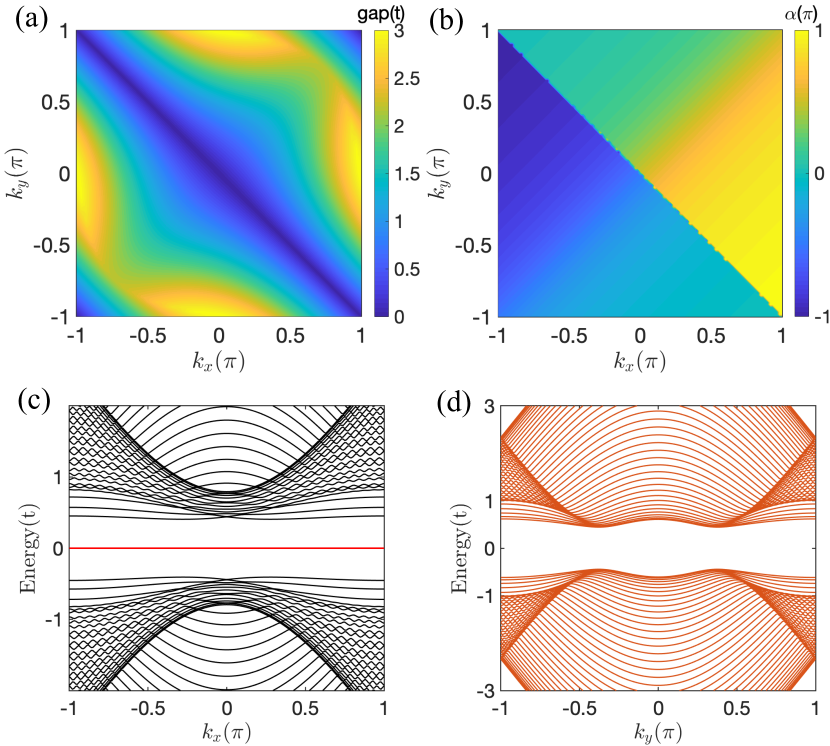
Figure 2: (a) Energy gap in the whole BZ for $t_{x}=t_{y}=0.5$. A gapless nodal line appears at the line $k_{x}+k_{y}=0$. (b) Angle $\alpha\equiv\mathrm{arg}[\varepsilon_{\eta=+1}({\bf k})]$ in the BZ for $t_{x}=t_{y}=0.5$. There is a branch cut at the line $k_{x}+k_{y}=0$. (c) Energy spectrum of a ribbon along $x$-direction with width $W_{y}=20$. Notice the flat band at zero energy. (d) Energy spectrum of the ribbons along $y$-direction with width $W_{x}=20$. Here we choose $t_{x}=1.2t,t_{y}=1.8t$ such that $w_{x}=0,w_{y}=1$.

V Topological phase transitions with merging of Dirac points

The mergence of two Dirac points undergoes a topological phase transition in our model. The semimetal phase with a pair of Dirac points locates in the shadowed region $|t_{x}+t_{y}|<2t$ and $t_{x}\neq t_{y}$ of Fig. 1(d). The topological phase transition after merging a pair of Dirac points transforms the semimetal phase to either a weak topological insulator or a nodal-line semimetal. Thus, our inclined 2D SSH model actually possesses three different topological phases, as shown in the phase diagram in Fig. 1(d). Let us first focus on the nodal-line semimetal phase under the specific condition $t_{x}=t_{y}$ [Fig. 1(d) and Fig. 2(a)]. Consider a representative phase point $A$ (or $B$) in the semimetal phase with a pair of Dirac points [see Fig. 1(d)]. As it moves towards the orange line, the Dirac points merge and we observe that the system exhibits a gapless nodal line at

$$k_{x}+k_{y}=0,\ \mathrm{if}\ t_{x}=t_{y}\neq t,$$ (8)

The appearance of a gapless nodal line is a direct consequence of an accidental mirror symmetry. Under the condition $t_{x}=t_{y}$, the system has mirror symmetry along the direction $x+y=0$. In momentum space, we thus transform the Hamiltonian as $MH(k_{x},k_{y})M^{-1}=H(-k_{y},-k_{x})$ where the mirror operator is given by $M=\left(\begin{array}[]{cc}\sigma_{x}&0\\ 0&\sigma_{0}\end{array}\right)$. Note that the Hamiltonian $H({\bf k})$ commutes with the mirror operator $M$ along the nodal-line $k_{x}+k_{y}=0$. Therefore, we can label the eigen states of the Hamiltonian $H({\bf k})$ by the eigen states $|\pm\rangle$ of the mirror operator $M$ as $H({\bf k})|\pm\rangle=\pm E|\pm\rangle$. We further note that the mirror operator commutes with the chiral symmetry operator, i.e., $[\mathcal{C},M]=0$. Therefore, we can show that $\mathcal{C}|+\rangle$ is also an eigenstate of $M$ with eigenvalue $+1$. Moreover, $\mathcal{C}|+\rangle$ is an eigenstate of $H({\bf k})$ with energy $+E$. Actually, chiral symmetry maps the state $|+\rangle$ with energy $+E$ to the state $\mathcal{C}|+\rangle$ with energy $-E$. This implies that those states are degenerate at $E=0$.

The nodal-line semimetal phase is protected by a topological invariant $\delta$ as we describe below. Let us define an angle $\alpha$ as $\alpha({\bf k})\equiv\mathrm{arg}[\varepsilon_{\eta=+1}({\bf k})]$ where $\varepsilon_{\eta}({\bf k})$ is defined below Eq. (3). In the nodal-line semimetal phase, $\varepsilon_{\eta=+1}({\bf k})=(t+t_{x})(\cos\frac{k_{x}}{2}-\cos\frac{k_{y}}{2})+i(t-t_{x})(\sin\frac{k_{x}}{2}+\sin\frac{k_{y}}{2}).$ Figure 2(a) plots the band gap in the whole BZ, which clearly shows a nodal-line along $k_{x}=-k_{y}$. Figure 2(b) shows the angle $\alpha$ in the BZ in the nodal-line semimetal phase. The branch cut at $k_{x}+k_{y}=0$ separates the BZ into two equal sections. Consider two mirror-symmetric wave-vectors ${\bf k}_{1}$ and ${\bf k}_{2}$ with respect to the line $k_{x}+k_{y}=0$. Consequently, the relation $\alpha({\bf k}_{1})=\alpha({\bf k}_{2})+(2N+1)\pi$ with $N$ integer holds. Thus, the topological invariant $\delta$ can be defined as $\delta\equiv[\alpha({\bf k}_{1})-\alpha({\bf k}_{2})]/\pi\ \mathrm{mod}\ 2$. This topological invariant $\delta$ is protected by mirror symmetry and is not affected by the gauge degrees of freedom of $\varepsilon_{\eta}({\bf k})$. In the case of Figs. 2(a) and 2(b), it is found that $\delta=1$.

Again, we consider a representative phase point $A$ (or $B$) in the semimetal phase in Fig. 1(d). As it moves parallel to the orange line, two Dirac points merge at the phase boundary $|t_{x}+t_{y}|=2t$. Similar to the case of graphene, the energy spectrum stays linear along one direction while it becomes parabolic along another direction at the critical merging points Montambaux et al. (2009). Interestingly, this topological phase transition gives rise to a weak topological insulator rather than a trivial insulator (see the representative phase points $C$ and D). The weak topological insulators are located in the region $|t_{x}+t_{y}|>2t$ and $t_{x}\neq t_{y}$. They are described by two winding numbers $(w_{x},w_{y})$ with one of them being one and the other one being zero. The winding number is defined as $w_{x/y}=\frac{1}{2\pi i}\int_{0}^{2\pi}dk_{x/y}\mathrm{Tr}[q^{-1}({\bf k})\partial_{k_{x/y}}q({\bf k})]$ for arbitrary $k_{y/x}\in[0,2\pi]$. Actually, this anisotropic topological insulating phase can be further divided into two subphases: (i) $w_{x}=1,w_{y}=0$ ($t_{x}>t_{y}$ and $|t_{x}+t_{y}|>2t$) and (ii) $w_{x}=0,w_{y}=1$ ($t_{x}<t_{y}$ and $|t_{x}+t_{y}|>2t$). When $w_{x}=1,w_{y}=0$ ($w_{x}=0,w_{y}=1$), the system is nontrivial along $x$($y$)-direction and trivial along $y(x)$-direction. Correspondingly, a totally flat edge band exists in the gap of the energy spectrum along $x$($y$)-direction for the subphase (i) (subphase (ii)) [see, for instance, Figs. 2(c,d)]. Notably, neither the topologically trivial phase with $w_{x}=w_{y}=0$ nor the topologically nontrivial phase with $w_{x}=w_{y}=1$ appear in the inclined 2D SSH model.

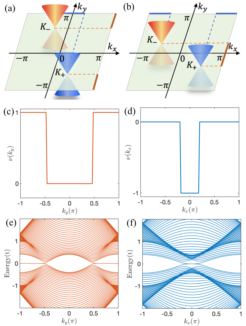
Figure 3: Anisotropic projection of the two Dirac points. (a) Schematic of anisotropic projection of bulk spectrum with two Dirac points (${\bf K}_{\pm}$) to $x$- and $y$-directions under the condition $t_{x}<t_{y}$. The dashed lines represent the projection direction. The thick solid lines (blue and red) at the boundary of the BZ indicate the nontrivial regions with flat edge bands. (b) Alternative projection similar to the case in (a) but under the condition $t_{x}>t_{y}$. (c) Winding number $\nu(k_{y})$ as a function of $k_{y}$. (d) Winding number $\nu(k_{x})$ as a function of $k_{x}$. (e) Energy spectrum of a ribbon along $y$-direction with width $W_{x}=20$ corresponding to the case in panel (c). Notice the flat band at zero energy. (f) Energy spectrum of the ribbons along $x$-direction with width $W_{y}=20$ corresponding to the the case in panel (d). In panels (c,d,e,f), the other parameters are $t_{x}=0.3t$ and $t_{y}=0.7t$, i.e., corresponding to the case in (a).

VI Anisotropic projection of Dirac points

The projection of two Dirac points to different directions shows two patterns as illustrated in Figs. 3(a) and 3(b). These two patterns can be described by the representative phase points $A$ and $B$ in Fig. 1(d), respectively. To switch between the two possible patterns, a phase point has to cross the gapless nodal-line semimetal phase. For simplicity, let us focus on the pattern in Fig. 3(a). When projecting the system along $x(y)$-direction, the same region in the BZ can be viewed as topologically nontrivial or trivial depending on relative values of $t_{x}$ and $t_{y}$ [see, for instance, Fig. 3(a) for $t_{x}<t_{y}$]. This anisotropic nature in our model suggests two independent indexes $\nu(k_{x})$ and $\nu(k_{y})$. Explicitly, they are given by

$$\nu(k_{x/y}) =\frac{1}{2\pi}\int_{0}^{2\pi}dk_{y/x}\frac{t^{2}e^{\mp ik_{y/x}}-t_{y/x}^{2}e^{\pm ik_{y/x}}}{R({\bf k})},$$ (9)

where $R({\bf k})\equiv(te^{ik_{x}/2}+t_{x}e^{-ik_{x}/2})^{2}-(te^{-ik_{y}/2}+t_{y}e^{ik_{y}/2})^{2}$. In essence, $\nu(k_{x/y})$ is a winding number of the reduced one-dimensional system at specific wave-number $k_{x/y}$ Shen et al. (2017); Li (2019). In Fig. 3(c), the middle region is trivial ($\nu=0$) while the two outer regions are nontrivial ($\nu=1$). It is interesting to see that this pattern is in stark contrast to that of Fig. 3(d), i.e., $\nu=-1$ in the middle region and $\nu=0$ otherwise. This difference comes from the anisotropic nature of the alternating dimerization pattern in our system. The nontrivial winding number indicates the existence of flat edge bands at open boundaries Ryu and Hatsugai (2002); Delplace et al. (2011); Shen et al. (2017); Li (2019). Evidently, the regions of flat bands in Figs. 3(e) and 3(f) agree with the topological nontrivial regions in Figs. 3(c) and 3(d), respectively.

VII Discussion and conclusion

To realize the inclined 2D SSH model experimentally, it needs a square lattice geometry (four sites in a unit cell) and controllable nearest-neighbor couplings. Required techniques for designing such a lattice structure have been developed in synthetic quantum materials such as photonic and acoustic crystals Wang et al. (2009); Xie et al. (2019); Chen et al. (2019); Serra-Garcia et al. (2018); Ni et al. (2019), electric circuits Imhof et al. (2018), and waveguides Peterson et al. (2018); Cerjan et al. (2020). For instance, to realize our model in a photonic waveguide system, waveguides can be arranged to a square lattice with four waveguides contained in each unit cell and the alternately dimerized couplings between neighboring waveguides can be modulated by their spacings Cerjan et al. (2020); El Hassan et al. (2019). Notably, our inclined 2D SSH model does not require delicate manipulations of external flux, differently from recent reports to realize Dirac states on square lattices Xue et al. (2021); Li et al. (2021b); Shao et al. (2021). These proposals require external $\pi$ fluxes, and the Dirac points are pinned at boundaries of the BZ.

Our model has a richer topological phase space accompanied with corresponding topological phase transitions as compared to artificial graphene Tarruell et al. (2012). In a special limit, our model reduces to the brick-type lattice model mimicking artificial graphene Wakabayashi et al. (1999) (see Appendix S4). Moreover, the realization of our model on a square lattice is simpler than the Mielke checkerboard model Mielke (1992) since it only involves nearest-neighbor hopping terms. We notice that similar 2D WTIs are discussed in related works Li et al. (2018); Jeon et al. (2022); Yang et al. (2022) but no nodal-line phase is mentioned therein. Interestingly, our model may provide a platform to realize the toric-code insulator Tam et al. (2022).

In conclusion, we have proposed an inclined 2D SSH model on a square lattice to realize highly tunable Dirac states. We have found that the locations of Dirac points are not pinned to any high-symmetry points or lines in the BZ but movable by parameter modifications. The mergence of two Dirac points leads to a topological phase transition, which converts the system from a semimetal phase with a pair of Dirac points to either a weak topological insulator or a nodal-line semimetal. We expect that our model can be realized in different metamaterial platforms.

VIII Acknowledgement

This work was supported by the DFG (SPP1666 and SFB1170 “ToCoTronics”), the Würzburg-Dresden Cluster of Excellence ct.qmat, EXC2147, Project-id 390858490, the Elitenetzwerk Bayern Graduate School on “Topological Insulators”, and the High Tech Agenda Bayern.

Appendix S1 Properties of the inclined 2D SSH model

In this appendix, we present the energy spectrum, Dirac points, and phase diagram of the inclined 2D SSH model.

A Energy spectrum

Let us calculate the spectrum of Hamiltonian Eq. (1) in the main text. To do so, we utilize the general properties of chiral symmetry. In the proper space, chiral symmetry can be expressed as $\tau_{3}H({\bf k})\tau_{3}=-H({\bf k})$. If we consider the eigen equation

$$H({\bf k})\Psi_{n} =E_{n}({\bf k})\Psi_{n},\ \Psi_{n}=\frac{1}{\sqrt{2}}\left(\begin{array}[]{c}\psi_{n}^{A}\\ \psi_{n}^{B}\end{array}\right),$$ (S1.3)

where $\psi_{n}^{A}$ and $\psi_{n}^{B}$ are the states referring to $A$ and $B$ sublattices, respectively, then, due to chiral symmetry, there is another state $\mathcal{C}\Psi_{n}$ satisfying the eigen equation $H({\bf k})[\mathcal{C}\Psi_{n}]=-E_{n}({\bf k})[\mathcal{C}\Psi_{n}].$ Squaring the Hamiltonian $H({\bf k})$, this yields

$$H^{2}({\bf k})\Psi_{n} =E_{n}^{2}({\bf k})\Psi_{n}.$$ (S1.4)

Explicitly, we effectively decouple the equation as

$$h_{A}({\bf k})\psi_{n}^{A} =E_{n}^{2}\psi_{n}^{A},\ \ h_{A}({\bf k})\equiv q({\bf k})q^{\dagger}({\bf k}),$$ (S1.5)

$$h_{B}({\bf k})\psi_{n}^{B} =E_{n}^{2}\psi_{n}^{B},\ \ h_{B}({\bf k})\equiv q^{\dagger}({\bf k})q({\bf k}).$$ (S1.6)

Note that $q({\bf k})$ is not necessarily Hermitian, while the two defined operators $h_{A}({\bf k})$ and $h_{B}({\bf k})$ are Hermitian.

For our model, we obtain

$$h_{A}({\bf k}) =h_{0}({\bf k})\sigma_{0}+h_{1}({\bf k})\left(\begin{array}[]{cc}0&e^{i(p_{x}+p_{y})}\\ e^{-i(p_{x}+p_{y})}&0\end{array}\right),$$ (S1.9)

$$h_{0}({\bf k}) =t^{2}+2t_{x}t\cos k_{x}+t_{x}^{2}+t^{2}+2t_{y}t\cos k_{y}+t_{y}^{2},$$ (S1.10)

$$h_{1}({\bf k}) =2(t+t_{x})(t+t_{y})\cos p_{x}\cos p_{y}$$

$$-2(t-t_{x})(t-t_{y})\sin p_{x}\sin p_{y},$$ (S1.11)

where $\ p_{x}\equiv\frac{k_{x}}{2},p_{y}\equiv\frac{k_{y}}{2}$. Thus, the energy of the system is

$$E_{\eta}^{\pm}({\bf k}) =\pm\sqrt{h_{0}({\bf k})+\eta h_{1}({\bf k})}\equiv\pm|\varepsilon_{\eta}({\bf k})|.$$ (S1.12)

We have defined that

$$\varepsilon_{\eta}({\bf k}) \equiv te^{ip_{x}}+t_{x}e^{-ip_{x}}+\eta[te^{-ip_{y}}+t_{y}e^{ip_{y}}].$$ (S1.13)

Then, the eigen states for $h_{A}({\bf k})$ can be simply written as

$$\psi_{\eta}^{A} =\frac{1}{\sqrt{2}}\left(\begin{array}[]{c}1\\ \eta e^{-i(p_{x}+p_{y})}\end{array}\right).$$ (S1.16)

Similar procedures can be applied to the operator $h_{B}({\bf k})$ to obtain the eigen states $\psi_{\eta}^{B}$. Therefore, the total wave function for $H({\bf k})$ is

$$\Psi_{\eta}^{\pm} =\frac{1}{\sqrt{2}}\left(\begin{array}[]{c}\psi_{\eta}^{A}\\ \pm\psi_{\eta}^{B}\end{array}\right)=\frac{1}{2}\left(\begin{array}[]{c}1\\ \eta e^{-i(p_{x}+p_{y})}\\ \pm 1\\ \pm\eta e^{-i(p_{y}-p_{x})}\end{array}\right).$$ (S1.23)

B Dirac points

Due to chiral symmetry, the conduction bands and valence bands touch at $E=0$. For the general case $t_{x}\neq t_{y}$, it requires the constraint $|\varepsilon_{\eta}({\bf k})|=0$ to have Dirac points, which implies the conditions

$$(t-t_{x})\sin p_{x}+\eta(t-t_{y})\sin p_{y}=0,$$ (S1.24)

$$(t+t_{x})\cos p_{x}-\eta(t+t_{y})\cos p_{y}=0.$$ (S1.25)

Further simplifying these equations, we can identify the locations of the Dirac point at ${\bf K}_{\pm}=\pm(K_{x},-K_{y})$ with

$$K_{x} =2\arccos\sqrt{\frac{(t+t_{y})^{2}(2t-t_{x}-t_{y})}{4t(t^{2}-t_{x}t_{y})}},$$ (S1.26)

$$K_{y} =2\arccos\sqrt{\frac{(t+t_{x})^{2}(2t-t_{x}-t_{y})}{4t(t^{2}-t_{x}t_{y})}}.$$ (S1.27)

The Dirac points are characterized by topological charges $Q_{{\bf K}_{\pm}}$ that can be calculated with the formula

$$Q_{{\bf K_{\pm}}}=\frac{1}{2\pi i}\oint_{\ell}d{\bf k}\cdot\mathrm{Tr}\left[q^{-1}({\bf k})\nabla_{{\bf k}}q({\bf k})\right],$$ (S1.28)

where the loop $\ell$ is chosen such that it encircles a single Dirac point ${\bf K}_{\pm}$. Then, we obtain

$$Q_{{\bf K_{\pm}}} =\frac{1}{2\pi}\oint_{\ell}dk_{x}\frac{e^{ik_{x}}t^{2}-t_{x}^{2}e^{-ik_{x}}}{R(k_{x},k_{y})}$$

$$+\frac{1}{2\pi}\oint_{\ell}dk_{y}\frac{e^{-ik_{y}}t^{2}-t_{y}^{2}e^{ik_{y}}}{R(k_{x},k_{y})}.$$ (S1.29)

We find that for any loop enclosing a single Dirac point, we get a nonzero topological charge $Q_{{\bf K_{\pm}}}=\pm 1$.

C Phase diagram

Our inclined 2D SSH model experiences three different phases: (i) semimetal phase with Dirac points; (ii) nodal-line semimetal phase; (iii) weak topological insulator phase. Let us further specify the three phases below.

Phase (i): To obtain Dirac points, we consider the ranges of $\cos^{2}p_{x}$ and $\cos^{2}p_{y}$ as

$$0<\frac{(t+t_{y})^{2}(2t-t_{x}-t_{y})}{4t(t^{2}-t_{x}t_{y})}<1$$ , (S1.30)

$$0<\frac{(t+t_{x})^{2}(2t-t_{x}-t_{y})}{4t(t^{2}-t_{x}t_{y})}<1$$ . (S1.31)

The conditions $\cos^{2}p_{x}>0$ and $\cos^{2}p_{y}>0$ lead to the inequalities

$$(a):\begin{cases}2t-t_{x}-t_{y}>0,\\ t^{2}-t_{x}t_{y}>0;\end{cases} b):\begin{cases}2t-t_{x}-t_{y}<0,\\ t^{2}-t_{x}t_{y}<0.\end{cases}$$ (S1.32)

For the first case (a), if we further assume $t>|(t_{x}+t_{y})/2|$, then $t^{2}>[(t_{x}+t_{y})/2]^{2}$. From the famous inequality that $[(a+b)/2]^{2}\geq ab$ for any $a,b$, the condition $t^{2}>t_{x}t_{y}$ is always satisfied. Otherwise, if $t<|(t_{x}+t_{y})/2|$, the second condition $t^{2}>t_{x}t_{y}$ is not always satisfied. For the second case (b), since $t>0$, we need $(t_{x}+t_{y})/2>0$. Therefore, the two conditions are not always compatible.

We further need

$$\frac{(t+t_{y})^{2}(2t-t_{x}-t_{y})}{4t(t^{2}-t_{x}t_{y})}<1.$$ (S1.33)

It can be proven that in the regime $2t>|t_{x}+t_{y}|$ we have $t^{2}-t_{x}t_{y}>0$ and $2t-(t_{x}+t_{y})>0.$ The above condition is equivalent to $(t-t_{y})^{2}(2t+t_{x}+t_{y})>0$, which is also naturally true in the region $2t>|t_{x}+t_{y}|$. Therefore, the semi-metallic phase with Dirac points appear for

$$2t>|t_{x}+t_{y}|.$$ (S1.34)

Phase (ii): From the unique form of energy spectrum, it is clear that the system has a gapless nodal line at

$$k_{x}+k_{y}=0,\ \mathrm{if}\ t_{x}=t_{y}\neq t.$$ (S1.35)

The appearance of a gapless nodal line is due to an accidental mirror symmetry.

Phase (iii): The weak topological insulator phase appears in the region $|t_{x}+t_{y}|>2t$ and $t_{x}\neq t_{y}$. The phase boundary between weak topological insulator and semimetal phase is located at $|t_{x}+t_{y}|=2t$.

Appendix S2 Anisotropic Fermi velocity at Dirac points

The effective Fermi velocity $v$ of the Dirac points in our model can also be manipulated by parameter modulations. The effective Fermi velocity plays a crucial role in characterizing the transport properties of Dirac states. Let us define an angle $\theta$ between the wave-vector ${\bf k}$ and the $+\hat{k}_{x}$ axis. As shown in Fig. 4(a), the anisotropic Fermi velocity shows sinusoidal behavior with respect to the angle $\theta$, consistent with elliptical Dirac cones in the two-band effective model around ${\bf K}_{\pm}$. As tuning $t_{x}$ and $t_{y}$, the Fermi velocity in different directions $\theta$ may change substantially [Fig. 4(b)]. Interestingly, the velocities along different directions coincide when $t_{x}=-t_{y}\simeq\pm 0.3t$, which indicates that the Dirac cones become isotropic.

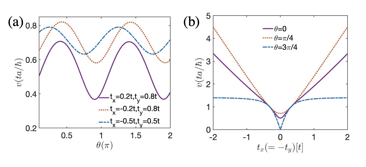
Figure 4: (a) Anisotropy of the Fermi velocity at the Dirac point ${\bf K_{+}}$ as a function of the angle $\theta$ for different $t_{x}$ and $t_{y}$. Here, $\theta$ is defined as an angle between the wave-vector ${\bf k}$ and $+\hat{k}_{x}$ axis. (b) Anisotropy of the Fermi velocity at the Dirac point ${\bf K_{+}}$ as a function of $t_{x}(=-t_{y})$ for different angles $\theta$.

Appendix S3 Gap the Dirac points by perturbations

As we discussed in the main text, the stability of Dirac points is protected by space-time inversion symmetry. Indeed, if we add a staggered onsite potential, say $\Delta\tau_{3}\sigma_{0}$ with $\Delta$ indicating its strength, to break the glide-inversion symmetry, the Dirac points are removed and a bulk gap opens, as shown in Fig. 5(a). If we, however, consider another type of staggered onsite potential $\Delta\tau_{0}\sigma_{3}$, which breaks chiral symmetry, while it respects the glide-inversion symmetry, then the Dirac points remain intact [Fig. 5(b)].

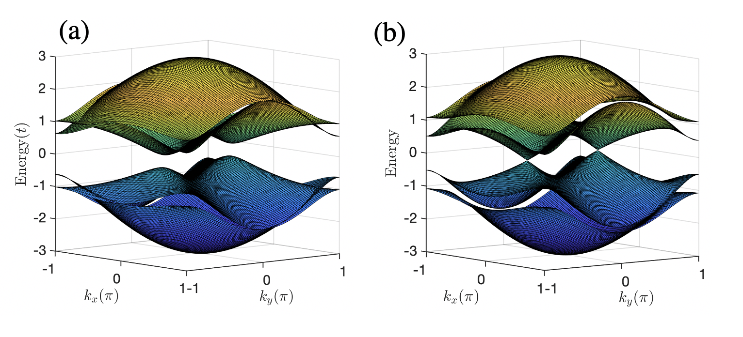
Figure 5: (a) Band structure of the inclined 2D SSH model with a pair of Dirac points being gapped by $\Delta\tau_{3}\sigma_{0}$ with $\Delta=0.1$. (b) Band structure of the inclined 2D SSH model with a pair of Dirac points under the perturbation term $\Delta\tau_{0}\sigma_{3}$ with $\Delta=0.1$. Other parameters are $t_{x}=0.2t$ and $t_{y}=0.8t$.

Appendix S4 Graphene limit

Here, we show that our inclined 2D SSH model can reduce to graphene (brick type lattice model) in a special limit. For instance, it is equivalent to a square lattice version of graphene when $t_{x}=t,t_{y}=0$. In Fig. 6(a), the six sites in the dashed square resemble the hexagon in graphene. Therefore, when projecting the system to $x$-direction, the Dirac points are located at $(\pm\frac{2\pi}{3},0)$ [see Fig. 6(b)]. For the spectrum along perpendicular direction, there are no flat edge bands [see Fig. 6(c)]. Similar results are obtained if we consider the limit $t_{x}=0,t_{y}=t$.

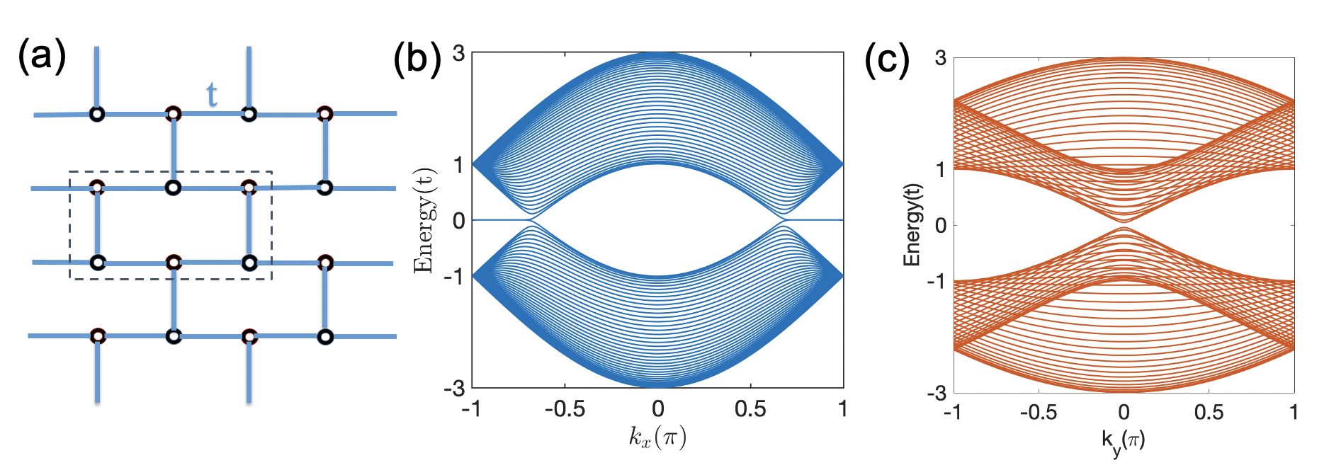
Figure 6: (a) Special limit of the inclined 2D SSH model with $t_{x}=t$ and $t_{y}=0$. (b) Spectrum of ribbon with finite width $W_{y}=20$ in the $y$-direction corresponds to panel (a). (c) Spectrum of ribbon with finite width $W_{x}=20$ in the $x$-direction corresponds to panel (a). The spectrum in (b) and (c) are totally the same as the spectrum of graphene ribbon with zigzag and armchair edges, respectively.

References

- Novoselov et al. (2005) K. S. Novoselov, A. K. Geim, S. V. Morozov, D. Jiang, M. I. Katsnelson, I. V. Grigorieva, S. V. Dubonos, and A. A. Firsov, Two-dimensional gas of massless Dirac fermions in graphene, Nature 438, 197 (2005).
- Castro Neto et al. (2009) A. H. Castro Neto, F. Guinea, N. M. R. Peres, K. S. Novoselov, and A. K. Geim, The electronic properties of graphene, Rev. Mod. Phys. 81, 109 (2009).
- Liu et al. (2011) C.-C. Liu, W. Feng, and Y. Yao, Quantum Spin Hall Effect in Silicene and Two-Dimensional Germanium, Phys. Rev. Lett. 107, 076802 (2011).
- Malko et al. (2012) D. Malko, C. Neiss, F. Viñes, and A. Görling, Competition for Graphene: Graphynes with Direction-Dependent Dirac Cones, Phys. Rev. Lett. 108, 086804 (2012).
- Young and Kane (2015) S. M. Young and C. L. Kane, Dirac Semimetals in Two Dimensions, Phys. Rev. Lett. 115, 126803 (2015).
- Zhang et al. (2005) Y. Zhang, Y.-W. Tan, H. L. Stormer, and P. Kim, Experimental observation of the quantum Hall effect and Berry’s phase in graphene, Nature 438, 201 (2005).
- Ando et al. (2002) T. Ando, Y. Zheng, and H. Suzuura, Dynamical Conductivity and Zero-Mode Anomaly in Honeycomb Lattices, J. Phys. Soc. Jap. 71, 1318 (2002).
- Tworzydło et al. (2006) J. Tworzydło, B. Trauzettel, M. Titov, A. Rycerz, and C. W. J. Beenakker, Sub-Poissonian Shot Noise in Graphene, Phys. Rev. Lett. 96, 246802 (2006).
- Katsnelson et al. (2006) M. I. Katsnelson, K. S. Novoselov, and A. K. Geim, Chiral tunnelling and the Klein paradox in graphene, Nat Phys 2, 620 (2006).
- Stander et al. (2009) N. Stander, B. Huard, and D. Goldhaber-Gordon, Evidence for Klein Tunneling in Graphene p n Junctions, Phys. Rev. Lett. 102, 026807 (2009).
- Pereira et al. (2009) V. M. Pereira, A. H. Castro Neto, and N. M. R. Peres, Tight-binding approach to uniaxial strain in graphene, Phys. Rev. B 80, 045401 (2009).
- Rycerz et al. (2007) A. Rycerz, J. Tworzydło, and C. W. J. Beenakker, Valley filter and valley valve in graphene, Nature Physics 3, 172 (2007).
- Xiao et al. (2007) D. Xiao, W. Yao, and Q. Niu, Valley-Contrasting Physics in Graphene: Magnetic Moment and Topological Transport, Phys. Rev. Lett. 99, 236809 (2007).
- Yao et al. (2008) W. Yao, D. Xiao, and Q. Niu, Valley-dependent optoelectronics from inversion symmetry breaking, Phys. Rev. B 77, 235406 (2008).
- Montambaux et al. (2009) G. Montambaux, F. Piéchon, J.-N. Fuchs, and M. O. Goerbig, Merging of Dirac points in a two-dimensional crystal, Phys. Rev. B 80, 153412 (2009).
- Feilhauer et al. (2015) J. Feilhauer, W. Apel, and L. Schweitzer, Merging of the Dirac points in electronic artificial graphene, Phys. Rev. B 92, 245424 (2015).
- Wunsch et al. (2008) B. Wunsch, F. Guinea, and F. Sols, Dirac-point engineering and topological phase transitions in honeycomb optical lattices, N. J. Phys. 10, 103027 (2008).
- Tarruell et al. (2012) L. Tarruell, D. Greif, T. Uehlinger, G. Jotzu, and T. Esslinger, Creating, moving and merging Dirac points with a Fermi gas in a tunable honeycomb lattice, Nature 483, 302 (2012).
- Bellec et al. (2013) M. Bellec, U. Kuhl, G. Montambaux, and F. Mortessagne, Topological Transition of Dirac Points in a Microwave Experiment, Phys. Rev. Lett. 110, 033902 (2013).
- Real et al. (2020) B. Real, O. Jamadi, M. Milicevic, and et., al., Semi-Dirac Transport and Anisotropic Localization in Polariton Honeycomb Lattices, Phys. Rev. Lett. 125, 186601 (2020).
- Su et al. (1979) W. P. Su, J. R. Schrieffer, and A. J. Heeger, Solitons in Polyacetylene, Phys. Rev. Lett. 42, 1698 (1979).
- Liu and Wakabayashi (2017) F. Liu and K. Wakabayashi, Novel Topological Phase with a Zero Berry Curvature, Phys. Rev. Lett. 118, 076803 (2017).
- Benalcazar et al. (2017a) W. A. Benalcazar, B. A. Bernevig, and T. L. Hughes, Quantized electric multipole insulators, Science 357, 61 (2017a).
- Benalcazar et al. (2017b) W. A. Benalcazar, B. A. Bernevig, and T. L. Hughes, Electric multipole moments, topological multipole moment pumping, and chiral hinge states in crystalline insulators, Phys. Rev. B 96, 245115 (2017b).
- Song et al. (2017) Z. Song, Z. Fang, and C. Fang, (d-2)-Dimensional Edge States of Rotation Symmetry Protected Topological States, Phys. Rev. Lett. 119, 246402 (2017).
- Schindler et al. (2018a) F. Schindler, A. M. Cook, M. G. Vergniory, Z. Wang, S. S. P. Parkin, B. A. Bernevig, and T. Neupert, Higher-order topological insulators, Science Advances 4 (2018a).
- Schindler et al. (2018b) F. Schindler, Z. Wang, M. G. Vergniory, A. M. Cook, A. Murani, S. Sengupta, A. Y. Kasumov, R. Deblock, S. Jeon, I. Drozdov, H. Bouchiat, S. Guéron, A. Yazdani, B. A. Bernevig, and T. Neupert, Higher-order topology in bismuth, Nat. Phys. 14, 918 (2018b).
- Imhof et al. (2018) S. Imhof, C. Berger, F. Bayer, J. Brehm, L. W. Molenkamp, T. Kiessling, F. Schindler, C. H. Lee, M. Greiter, T. Neupert, and R. Thomale, Topolectrical-circuit realization of topological corner modes, Nat. Phys. 14, 925 (2018).
- Serra-Garcia et al. (2018) M. Serra-Garcia, V. Peri, R. Süsstrunk, O. R. Bilal, T. Larsen, L. G. Villanueva, and S. D. Huber, Observation of a phononic quadrupole topological insulator, Nature 555, 342 (2018).
- Xie et al. (2019) B.-Y. Xie, G.-X. Su, H.-F. Wang, H. Su, X.-P. Shen, P. Zhan, M.-H. Lu, Z.-L. Wang, and Y.-F. Chen, Visualization of Higher-Order Topological Insulating Phases in Two-Dimensional Dielectric Photonic Crystals, Phys. Rev. Lett. 122, 233903 (2019).
- Chen et al. (2019) X.-D. Chen, W.-M. Deng, F.-L. Shi, F.-L. Zhao, M. Chen, and J.-W. Dong, Direct Observation of Corner States in Second-Order Topological Photonic Crystal Slabs, Phys. Rev. Lett. 122, 233902 (2019).
- Peterson et al. (2018) C. W. Peterson, W. A. Benalcazar, T. L. Hughes, and G. Bahl, A quantized microwave quadrupole insulator with topologically protected corner states, Nature 555, 346 (2018).
- Li et al. (2018) L. Li, M. Umer, and J. Gong, Direct prediction of corner state configurations from edge winding numbers in two- and three-dimensional chiral-symmetric lattice systems, Phys. Rev. B 98, 205422 (2018).
- Jeon et al. (2022) S. Jeon, and Y. Kim, Two-dimensional weak topological insulators in inversion-symmetric crystals, Phys. Rev. B 105, L121101 (2022).
- Zhang et al. (2020) R.-X. Zhang, F. Wu, and S. Das Sarma, Möbius Insulator and Higher-Order Topology in MnBiTe, Phys. Rev. Lett. 124, 136407 (2020).
- Li et al. (2020) C.-A. Li, B. Fu, Z.-A. Hu, J. Li, and S.-Q. Shen, Topological Phase Transitions in Disordered Electric Quadrupole Insulators, Phys. Rev. Lett. 125, 166801 (2020).
- Wei et al. (2021) Q. Wei, X. Zhang, W. Deng, J. Lu, X. Huang, M. Yan, G. Chen, Z. Liu, and S. Jia, 3D Hinge Transport in Acoustic Higher-Order Topological Insulators, Phys. Rev. Lett. 127, 255501 (2021).
- Li and Wu (2020) C.-A. Li and S. S. Wu, Topological states in generalized electric quadrupole insulators, Phys. Rev. B 101, 195309 (2020).
- Zhang and Trauzettel (2020) S.-B. Zhang and B. Trauzettel, Detection of second-order topological superconductors by Josephson junctions, Phys. Rev. Research 2, 012018 (2020).
- Li et al. (2021a) C.-A. Li, S.-B. Zhang, J. Li, and B. Trauzettel, Higher-Order Fabry-Pérot Interferometer from Topological Hinge States, Phys. Rev. Lett. 127, 026803 (2021a).
- Schnyder et al. (2008) A. P. Schnyder, S. Ryu, A. Furusaki, and A. W. W. Ludwig, Classification of topological insulators and superconductors in three spatial dimensions, Phys. Rev. B 78, 195125 (2008).
- Schnyder and Ryu (2011) A. P. Schnyder and S. Ryu, Topological phases and surface flat bands in superconductors without inversion symmetry, Phys. Rev. B 84, 060504 (2011).
- Heikkilä et al. (2011) T. T. Heikkilä, N. B. Kopnin, and G. E. Volovik, Flat bands in topological media, JETP Letters 94, 233 (2011).
- Fang and Fu (2015) C. Fang and L. Fu, New classes of three-dimensional topological crystalline insulators: Nonsymmorphic and magnetic, Phys. Rev. B 91, 161105 (2015).
- Kim et al. (2017) J. Kim, S. S. Baik, S. W. Jung, Y. Sohn, S. H. Ryu, H. J. Choi, B.-J. Yang, and K. S. Kim, Two-Dimensional Dirac Fermions Protected by Space-Time Inversion Symmetry in Black Phosphorus, Phys. Rev. Lett. 119, 226801 (2017).
- Shen et al. (2017) S.-Q. Shen, C.-A. Li, and Q. Niu, Chiral anomaly and anomalous finite-size conductivity in graphene, 2D Materials 4, 035014 (2017).
- Li (2019) C.-A. Li, Pseudo chiral anomaly in zigzag graphene ribbons, J. Phys.: Condens. Matter 32, 025301 (2019).
- Ryu and Hatsugai (2002) S. Ryu and Y. Hatsugai, Topological Origin of Zero-Energy Edge States in Particle-Hole Symmetric Systems, Phys. Rev. Lett. 89, 077002 (2002).
- Delplace et al. (2011) P. Delplace, D. Ullmo, and G. Montambaux, Zak phase and the existence of edge states in graphene, Phys. Rev. B 84, 195452 (2011).
- Wang et al. (2009) Z. Wang, Y. Chong, J. D. Joannopoulos, and M. Soljačić, Observation of unidirectional backscattering-immune topological electromagnetic states, Nature 461, 772 (2009).
- Ni et al. (2019) X. Ni, M. Weiner, A. Alù, and A. B. Khanikaev, Observation of higher-order topological acoustic states protected by generalized chiral symmetry, Nat. Mater. 18, 113 (2019).
- Cerjan et al. (2020) A. Cerjan, M. Jürgensen, W. A. Benalcazar, S. Mukherjee, and M. C. Rechtsman, Observation of a Higher-Order Topological Bound State in the Continuum, Phys. Rev. Lett. 125, 213901 (2020).
- El Hassan et al. (2019) A. El Hassan, F. K. Kunst, A. Moritz, G. Andler, E. J. Bergholtz, and M. Bourennane, Corner states of light in photonic waveguides, Nat. Photonics 13, 697 (2019).
- Xue et al. (2021) H. Xue, Z. Wang, Y.-X. Huang, Z. Cheng, L. Yu, Y. X. Foo, Y. X. Zhao, S. A. Yang, and B. Zhang, Projectively Enriched Symmetry and Topology in Acoustic Crystals, Phys. Rev. Lett. 128, 116802 (2022).
- Li et al. (2021b) T. Li, J. Du, Q. Zhang, Y. Li, X. Fan, F. Zhang, and C. Qiu, Acoustic Möbius Insulators from Projective Symmetry, Phys. Rev. Lett. 128, 116803 (2022).
- Shao et al. (2021) L. B. Shao, Q. Liu, R. Xiao, S. A. Yang, and Y. X. Zhao, Gauge-Field Extended k.p Method and Novel Topological Phases, Phys. Rev. Lett. 127, 076401 (2021).
- Wakabayashi et al. (1999) K. Wakabayashi, M. Fujita, H. Ajiki, and M. Sigrist, Electronic and magnetic properties of nanographite ribbons, Phys. Rev. B 59, 8271 (1999).
- Mielke (1992) A. Mielke, Exact ground states for the Hubbard model on the Kagome lattice, Journal of Physics A: Mathematical and General 25, 4335 (1992).
- Yang et al. (2022) H. Yang, L. Song, Y. Cao, and P. Yan, Experimental Realization of Two-Dimensional Weak Topological Insulators, Nano Lett. 22(7), 3125 (2022).
- Tam et al. (2022) P. M. Tam, J. W. F. Venderbos, and C. L. Kane, Toric-code insulator enriched by translation symmetry, Phys. Rev. B 105, 045106 (2022).