Theoretical predictions for inclusive $B\to X_{u}\tau\bar{\nu}$ decay

Abstract

With the expected large increase in data sets, previously not measured decays will be studied at Belle II. We derive standard model predictions for the $B\to X_{u}\tau\bar{\nu}$ decay rate and distributions. The region in the lepton energy spectrum where higher-dimension operators in the local OPE need to be resummed into the $b$-quark light-cone distribution function is a significantly greater fraction of the phase space than for massless leptons. The finite $\tau$ mass has the novel effect of shifting and squeezing how the distribution function enters the lepton energy spectrum. We also derive new predictions for the $\tau$ polarization.

I Introduction

The more than $3\sigma$ deviation of the measured $B\to D^{(*)}\tau\bar{\nu}$ rates [1, 2, 3, 4, 5, 6, 7, 8, 9] from the standard model (SM) predictions motivates the study of all possible semileptonic decays with $\tau$ leptons in the final state, both experimentally and theoretically. Comparisons of measured spectra and rates to different hadronic final states can give information on the structure of contributing four-fermion operators. Comparisons of $b\to c\ell\bar{\nu}$ and $b\to u\ell\bar{\nu}$ decays give constraints on the flavor structure of beyond standard model scenarios at play.

In this paper we study the inclusive decay $B\to X_{u}\tau\bar{\nu}$, which has been much less explored theoretically. Precise predictions for this decay are naturally interesting as a signal channel to measure in the future. In the near term, reliably modelling this decay as a background is interesting both to SM measurements and analyses aimed at more precisely measuring $R(D^{(*)})$ and clarifying the current tension with the SM. The Belle Collaboration set the first bound on a $b\to u\tau\bar{\nu}$ mediated decay, ${\cal B}(B\to\pi\tau\bar{\nu})<2.5\times 10^{-4}$ [10], at a level several times higher than SM predictions, and recent theoretical studies [11, 12, 13] also focused on exclusive decays.

Inclusive semileptonic decays of hadrons containing a heavy quark allow for a systematic expansion of nonperturbative effects in powers of $\Lambda_{\rm QCD}/m_{Q}$ [14]. The inclusive decay rates computed in the $m_{Q}\gg\Lambda_{\rm QCD}$ limit coincide with the free-quark decay rate, while corrections of order $\Lambda_{\rm QCD}/m_{Q}$ vanish [14, 15]. The leading nonperturbative corrections are of order $\Lambda_{\rm QCD}^{2}/m_{Q}^{2}$ and depend on only two hadronic quantities, $\lambda_{1}$ and $\lambda_{2}$, which describe certain forward matrix elements of local dimension-five operators. These corrections have been computed for a number of processes [16, 17, 18, 19, 20, 21, 22]. For $B\to X_{u}\tau\bar{\nu}$ decay, expressions for the total rate and leptonic $q^{2}$ spectra are straightforward to derive by taking the $m_{q}\to 0$ limit of the $B\to X_{c}\tau\bar{\nu}$ results [22, 23], but this limit is singular for the lepton energy spectrum and has not been given in the literature. Similarly, the perturbative ${\cal O}(\alpha_{s})$ corrections to the total $B\to X_{u}\tau\bar{\nu}$ semileptonic decay rate [24], the dilepton $q^{2}$ spectrum [25], and the doubly differential ${\rm d}\Gamma/{\rm d}q^{2}{\rm d}y$ spectrum [26, 27] are known analytically. However, no closed form expressions have thus far been derived for the ${\cal O}(\alpha_{s})$ corrections to the $\tau$ lepton energy spectrum. We present the results of the local OPE to ${\cal O}(\Lambda_{\rm QCD}^{2}/m_{b}^{2},\,\alpha_{s})$ in Sec. II.

Phase space regions in inclusive $B\to X_{u}e\bar{\nu}$ decay, when kinematic cuts restrict the invariant mass of the hadronic final state to be small (i.e., $m_{X}<m_{D}$), are relevant for the determination of $|V_{ub}|$. Decay rates in such regions are subject to large corrections, both perturbative and nonperturbative. In the region near maximal lepton energy the OPE breaks down and a resummation of the series of leading nonperturbative corrections is required [28, 29]. The lepton energy spectrum in a region of width $\Delta E_{\ell}\sim\Lambda_{\rm QCD}$ near the endpoint is determined by a nonperturbative $b$-quark distribution function in the $B$ meson. Similarly, the local OPE for $B\to X_{u}\tau\bar{\nu}$ breaks down near the endpoint of the $\tau$ energy spectrum; however, since in $B\to X_{u}\tau\bar{\nu}$ decay, $m_{\tau}<E_{\tau}<(m_{B}^{2}+m_{\tau}^{2})/(2m_{B})$ amounts to $1.78\,{\rm GeV}<E_{\tau}<2.94\,{\rm GeV}$, the distribution function is important over a much greater fraction of the available phase space than in $B\to X_{u}e\bar{\nu}$, where $0<E_{e}<m_{B}/2$. We consider the effects of the $b$-quark distribution function in Sec. III and explore its effect on the spectrum. Since the distribution of the measurable $\tau$ decay products (e.g., the charged lepton energy) are sensitive to the $\tau$ polarization, we also present results for decays to each polarization state.

To appreciate the mass suppressions in the decay rates, simply using the ${\cal O}(\Lambda_{\rm QCD}^{2}/m_{b}^{2})$ [20, 21, 22] and ${\cal O}(\alpha_{s})$ contributions [24, 22] in the $1S$ scheme [30, 31, 32], one finds [31]

$$\frac{\Gamma(B\to X_{u}\ell\bar{\nu})}{\Gamma(B\to X_{u}\tau\bar{\nu})}\,=2.97\,,\quad\frac{\Gamma(B\to X_{c}\ell\bar{\nu})}{\Gamma(B\to X_{c}\tau\bar{\nu})}\,=4.50\,,$$ (1)

Thus, the suppression of the rate due to finite $m_{\tau}$ is less strong in $b\to u$ than in $b\to c$ decays. Correspondingly, the suppression due to finite $m_{c}$ is clearly greater in $B\to\tau$ than in $B\to e$ semileptonic decays,

$$\frac{\Gamma(B\to X_{u}\tau\bar{\nu})}{\Gamma(B\to X_{c}\tau\bar{\nu})}\,\frac{|V_{cb}|^{2}}{|V_{ub}|^{2}} = 3.13\,,$$

$$\frac{\Gamma(B\to X_{u}\ell\bar{\nu})}{\Gamma(B\to X_{c}\ell\bar{\nu})}\,\frac{|V_{cb}|^{2}}{|V_{ub}|^{2}} = 1.83\,.$$ (2)

II local ope results

II.1 Nonperturbative Corrections

The inclusive $B\to X_{q}\,\ell\bar{\nu}$ decay ($q=u,c$ ; $\ell=e,\mu,\tau$) has been considered to order $1/m_{b}^{2}$ in the heavy quark expansion [20, 21, 22], including effects of the finite lepton mass. For $m_{q}=0$ the lepton energy spectrum becomes singular, and the limit must be taken with care. We find for $B\to X_{u}\tau\bar{\nu}$ decay,

$$\frac{1}{\Gamma_{u}}\frac{{\rm d}\Gamma}{{\rm d}y} = 2\sqrt{y^{2}-4\rho_{\tau}}\,\bigg{[}3y-2y^{2}-4\rho_{\tau}+3\rho_{\tau}y+\frac{\lambda_{2}}{m_{b}^{2}}\,6y$$ (3)

$${}+\frac{\lambda_{1}+3\lambda_{2}}{3m_{b}^{2}}\,(5y^{2}-14\rho_{\tau})\bigg{]}\,\theta(1+\rho_{\tau}-y)$$

$$- \bigg{[}\frac{\lambda_{1}}{3m_{b}^{2}}\,(1+\rho_{\tau})+\frac{\lambda_{2}}{m_{b}^{2}}\,(11-5\rho_{\tau})\bigg{]}$$

$${}\times(1-\rho_{\tau})^{3}\,\delta(1+\rho_{\tau}-y)$$

$$- \frac{\lambda_{1}}{3m_{b}^{2}}\,(1-\rho_{\tau})^{5}\,\delta^{\prime}(1+\rho_{\tau}-y)\,,$$

where we use the dimensionless variables

$$y=\frac{2E_{\tau}}{m_{b}}\,,\qquad\hat{q}^{2}=\frac{q^{2}}{m_{b}^{2}}\,,\qquad\rho_{\tau}=\frac{m_{\tau}^{2}}{m_{b}^{2}}\,,$$ (4)

and

$$\Gamma_{u}=\frac{|V_{ub}|^{2}\,G_{F}^{2}\,m_{b}^{5}}{192\,\pi^{3}}\,.$$ (5)

This agrees with the more complicated expression given in Ref. [21]. Here $\lambda_{1}$ and $\lambda_{2}$ are matrix elements in the heavy quark effective theory (HQET), defined by

$$\frac{1}{2m_{B}}\langle B|\,\bar{b}_{v}\,(iD)^{2}\,b_{v}|B\rangle = 2\,\lambda_{1}\,,$$

$$\frac{1}{2m_{B}}\langle B|\,\frac{g_{s}}{2}\,\bar{b}_{v}\,\sigma_{\mu\nu}G^{\mu\nu}\,b_{v}|B\rangle = 6\,\lambda_{2}\,,$$ (6)

and $b_{v}$ is the heavy $b$-quark field of HQET [34] with velocity $v$.

The $\tau$ can have spin up ($s=+$) or spin down ($s=-$) relative to the direction of its three-momentum, and it is convenient to decompose the corresponding decay rates as

$$\Gamma(B\to X_{u}\,\tau(s=\pm)\,\bar{\nu})=\frac{1}{2}\,\Gamma\pm\tilde{\Gamma}\,.$$ (7)

The rate, summed over the tau polarizations, is given by $\Gamma$, while the average tau polarization is $A_{\rm pol}=2\tilde{\Gamma}/\Gamma$. The $\tau$ polarization gives complementary sensitivity to BSM physics [35]. We obtain for its lepton energy dependence,

$$\frac{1}{\Gamma_{u}}\frac{{\rm d}\tilde{\Gamma}}{{\rm d}y} = -(y^{2}-4\rho_{\tau})\bigg{[}3-2y+\rho_{\tau}$$ (8)

$${}\quad+\frac{6\lambda_{2}}{m_{b}^{2}}+\frac{\lambda_{1}+3\lambda_{2}}{3m_{b}^{2}}5y\bigg{]}\,\theta(1+\rho_{\tau}-y)$$

$$+ \bigg{[}\frac{\lambda_{1}}{6m_{b}^{2}}\,(1-3\rho_{\tau})+\frac{\lambda_{2}}{2m_{b}^{2}}\,(11-5\rho_{\tau})\bigg{]}$$

$${}\quad\times(1-\rho_{\tau})^{3}\,\delta(1+\rho_{\tau}-y)$$

$$+ \frac{\lambda_{1}}{6m_{b}^{2}}\,(1-\rho_{\tau})^{5}\,\delta^{\prime}(1+\rho_{\tau}-y)\,.$$

Note that for $\rho_{\tau}=0$, $-2\,{\rm d}\tilde{\Gamma}={\rm d}\Gamma$, since the massless lepton is purely left-handed. Angular momentum conservation in $B\to X_{u}\tau\bar{\nu}$ implies that the $\tau$ polarization is fully left-handed at maximal $E_{\tau}$. This holds at the parton level to all orders in $\alpha_{s}$, and our results indeed satisfy it at order $\alpha_{s}^{0}$ and order $\alpha_{s}^{1}$; i.e., $\Gamma/2=-\tilde{\Gamma}$ at $y=1+\rho_{\tau}$. However, the power-suppressed terms that start at order $\Lambda_{\rm QCD}^{2}/m_{b}^{2}$ incorporate nonperturbative corrections between the $E_{\tau}$ endpoint at the parton level and at the hadron level. As a result, the physical rate at maximal $E_{\tau}$ vanishes (it is nonzero at the parton level). In a small region very close to the endpoint the most singular terms of the form $\lambda_{1}\,\delta^{\prime}(1+\rho_{\tau}-y)$ are the most important, and these also obey the $\Gamma/2=-\tilde{\Gamma}$ relation.

For ${\rm d}\Gamma/{\rm d}\hat{q}^{2}$, the $m_{q}\to 0$ limit the of $B\to X_{c}\tau\bar{\nu}$ expression is smooth, which gives the known result [23],

$$\frac{1}{\Gamma_{u}}\frac{{\rm d}\Gamma}{{\rm d}\hat{q}^{2}} = \frac{(\hat{q}^{2}-\rho_{\tau})^{2}}{\hat{q}^{6}}\bigg{\{}\bigg{(}1+\frac{\lambda_{1}}{2m_{b}^{2}}\bigg{)}2(1-\hat{q}^{2})^{2}$$

$${}\times\Big{[}\hat{q}^{2}(1+2\hat{q}^{2})+\rho_{\tau}(2+\hat{q}^{2})\Big{]}$$

$$+ \frac{3\lambda_{2}}{m_{b}^{2}}\Big{[}\hat{q}^{2}(1-15\hat{q}^{4}+10\hat{q}^{6})+\rho_{\tau}(2-3\hat{q}^{2}+5\hat{q}^{6})\Big{]}\!\bigg{\}}.$$

Integrating over phase space, the $B\to X_{u}\tau\bar{\nu}$ rate is

$$\frac{\Gamma}{\Gamma_{u}} = \bigg{(}1+\frac{\lambda_{1}}{2m_{b}^{2}}\bigg{)}\big{(}1-8\rho_{\tau}+8\rho_{\tau}^{3}-\rho_{\tau}^{4}-12\rho_{\tau}^{2}\ln\rho_{\tau}\big{)}$$

$$-\frac{3\lambda_{2}}{2m_{b}^{2}}\big{(}3-8\rho_{\tau}+24\rho_{\tau}^{2}-24\rho_{\tau}^{3}+5\rho_{\tau}^{4}+12\rho_{\tau}^{2}\ln\rho_{\tau}\big{)}\,,$$

and the polarization is given by

$$\frac{\tilde{\Gamma}}{\Gamma_{u}} = -\frac{(1-\hat{m}_{\tau})^{3}}{2}\bigg{[}\frac{(1-\hat{m}_{\tau})^{2}}{3}\,\big{(}3+15\hat{m}_{\tau}+5\hat{m}_{\tau}^{2}+\hat{m}_{\tau}^{3}\big{)}$$

$${}+\frac{\lambda_{1}}{6m_{b}^{2}}\,(1+\hat{m}_{\tau})^{3}\,(3+\hat{m}_{\tau}^{2})$$

$$-\frac{\lambda_{2}}{2m_{b}^{2}}\big{(}9+27\hat{m}_{\tau}+70\hat{m}_{\tau}^{2}+10\hat{m}_{\tau}^{3}-15\hat{m}_{\tau}^{4}-5\hat{m}_{\tau}^{5}\big{)}\bigg{]},$$

where $\hat{m}_{\tau}=\sqrt{\rho_{\tau}}$.

II.2 Perturbative Corrections

Analytic results for the doubly differential ${\rm d}\Gamma/{\rm d}q^{2}{\rm d}y$ spectra (including the $\tau$ polarization dependence) were given in Refs. [26, 27] , but only numerical results were presented for the $\tau$ energy spectrum. Integrating the doubly differential spectra over $q^{2}$ gives the charged lepton energy spectra for both unpolarized and polarized $\tau$ leptons. In the unpolarized case, writing

$$\frac{1}{\Gamma_{0}}\frac{{\rm d}\Gamma_{\tau}}{{\rm d}y}=\Big{[}F_{0}(y)-\frac{\alpha_{s}C_{F}}{2\pi}F_{1}(y)\Big{]}\,\theta(1+\rho_{\tau}-y)\,,$$ (12)

where $C_{F}=4/3$, we find

$$F_{0}(y)=2\sqrt{y^{2}-4\rho_{\tau}}\,\big{[}(3-2y)y+\rho_{\tau}(3y-4)\big{]}\,,$$ (13)

and

$$F_{1}(y)={} F_{0}(y)\left[\text{Li}_{2}(\tau_{+})+\text{Li}_{2}(\tau_{-})+4Y_{p}^{2}\right]+\left(6y^{2}-4y^{3}+6\rho_{\tau}y^{2}-12\rho_{\tau}^{2}\right)\left[\text{Li}_{2}(\tau_{+})-\text{Li}_{2}(\tau_{-})\right]$$ (14)

$$-2Y_{p}\left(\frac{5\rho_{\tau}^{3}}{3}+\rho_{\tau}(7y^{2}-6y+7)-6y^{3}+10y^{2}+\rho_{\tau}^{2}(4y-23)+6y-\frac{41}{3}\right)$$

$$+\sqrt{y^{2}-4\rho_{\tau}}\left(-\frac{34y^{2}}{3}+\rho_{\tau}\left(15y-\frac{74}{3}\right)+24y-6\right)\ln(1-y+\rho_{\tau})$$

$$+\sqrt{y^{2}-4\rho_{\tau}}\left(21\rho_{\tau}^{2}+\frac{1}{6}\left[\left(86-16\pi^{2}\right)y^{2}+\left(24\pi^{2}-153\right)y+82\right]+\frac{\rho_{\tau}}{6}\left(24\pi^{2}y-167y-32\pi^{2}+64\right)\right),$$

where $Y_{p}=\frac{1}{2}\ln[(1-\tau_{+})/(1-\tau_{-})]$ is the rapidity of all decay products (combined) against which the $\tau$ recoils, and

$$\tau_{\pm}=\frac{1}{2}\left(y\pm\sqrt{y^{2}-4\rho_{\tau}}\right).$$ (15)

Similarly, defining the polarization dependence of the lepton energy spectrum as

$$\frac{{\rm d}\Gamma^{\pm}_{\tau}}{{\rm d}y}=\frac{1}{2}\frac{{\rm d}\Gamma_{\tau}}{{\rm d}y}\pm\frac{{\rm d}\tilde{\Gamma}_{\tau}}{{\rm d}y}\,,$$ (16)

we write the polarization dependence of the rate to produce a $\tau$ lepton as

$$\frac{1}{\Gamma_{0}}\frac{{\rm d}\tilde{\Gamma}_{\tau}}{{\rm d}y}=\Big{[}\tilde{F}_{0}(y)-\frac{\alpha_{s}C_{F}}{2\pi}\tilde{F}_{1}(y)\Big{]}\,\theta(1+\rho_{\tau}-y)\,.$$ (17)

At tree level,

$$\tilde{F}_{0}(y)=\left(y^{2}-4\rho_{\tau}\right)(2y-3-\rho_{\tau})\,,$$ (18)

while at one loop,

$$\tilde{F}_{1}(y)={} \tilde{F}_{0}(y)\left[\text{Li}_{2}(\tau_{+})+\text{Li}_{2}(\tau_{-})+4Y_{p}^{2}\right]+\frac{12\rho_{\tau}^{2}-\rho_{\tau}\left(y^{3}+6y^{2}-6y\right)+2y^{4}-3y^{3}}{\sqrt{y^{2}-4\rho_{\tau}}}\left[\text{Li}_{2}(\tau_{+})-\text{Li}_{2}(\tau_{-})\right]$$

$$-\frac{Y_{p}}{3\sqrt{y^{2}-4\rho_{\tau}}}\bigg{[}\rho_{\tau}\left(y^{3}-210y^{2}+405y-260\right)+\left(18y^{4}-12y^{3}-36y^{2}+41y\right)+\rho_{\tau}^{3}(y-24)+\rho_{\tau}^{2}(93y-12)\bigg{]}$$

$$+\left[\frac{34\rho_{\tau}^{2}}{3}+\rho_{\tau}\left(-\frac{23y^{2}}{6}-\frac{53y}{3}+30\right)+\frac{17y^{3}}{3}-9y^{2}\right]\ln(1-y+\rho_{\tau})+\frac{\rho_{\tau}^{3}}{3}+\rho_{\tau}^{2}\left(-\frac{11y}{6}+\frac{8\pi^{2}}{3}-21\right)$$

$$+\frac{\rho_{\tau}}{12}\left(-8\pi^{2}y^{2}+149y^{2}-64\pi^{2}y-48y+96\pi^{2}+32\right)+\frac{1}{12}\left(16\pi^{2}y^{3}-86y^{3}-24\pi^{2}y^{2}+153y^{2}-82y\right).$$ (19)

III The lepton energy endpoint region

Near the endpoint of the lepton energy spectrum $y\sim 1+\rho_{\tau}$, a class of higher-order terms in the local OPE in Eq. (3) is no longer suppressed, and instead the differential rate is given by a nonlocal OPE in terms of the light-cone momentum distribution function of the $b$ quark [36, 28, 37, 38, 29, 39].

This endpoint region has been extensively studied in the context of massless leptons. It is straightforward to extend this to nonzero $\tau$ mass. At the parton level the lepton energy endpoint is determined by the $\theta$ function

$$\theta\big{(}(p_{b}-p_{\tau})^{2}\big{)}=\theta\left(m_{b}^{2}+m_{\tau}^{2}-2\,p_{\tau}\cdot p_{b}\right).$$ (20)

Writing

$$p_{\tau}^{\mu}=\frac{m_{b}}{2}\big{(}\tau_{-}\,n^{\mu}+\tau_{+}\,\bar{n}^{\mu}\big{)}\,,$$ (21)

where $\tau_{\pm}$ are given in Eq. (15), defines the light-like vectors $n^{\mu}$ and $\bar{n}^{\mu}=2v^{\mu}-n^{\mu}$. Taking $p_{b}^{\mu}=m_{b}v^{\mu}+k^{\mu}$, expanding in powers of $k^{\mu}/m_{b}$ and applying the HQET onshell condition $k\cdot v=0$, the $\theta$ function becomes

$$\theta\left(1+\rho_{\tau}-y+\frac{k\cdot n}{m_{b}}\,\sqrt{y^{2}-4\rho_{\tau}}+{\cal O}(k^{2})\right).$$ (22)

Over most of the spectrum, the ${\cal O}(k\cdot n)$ term may be neglected at leading order in $1/m_{b}$ and we recover the OPE result in Eq. (3). However, when $E_{\tau}$ is near the partonic endpoint, i.e., $1+\rho_{\tau}-y={\cal O}(\Lambda_{\rm QCD}/m_{b})$, $p_{b}-p_{\tau}$ approaches a light-like vector in the $n$ direction. In this region the ${\cal O}(k\cdot n)$ term is the same order as the leading term, and so must be included in the leading-order expression. Defining

$$\Delta\equiv\frac{1+\rho_{\tau}-y}{1-\rho_{\tau}}\,,$$ (23)

taking $\Delta\sim{\cal O}(\Lambda_{\rm QCD}/m_{b})$, and expanding (22) in powers of $\Delta$ then gives

$$\theta\bigg{(}\Delta+\frac{k\cdot n}{m_{b}}\bigg{)}+{\cal O}(\Lambda_{\rm QCD}/m_{b})\,.$$ (24)

Comparing with the $\rho_{\tau}\to 0$ limit, the nonzero $\tau$ mass shifts the endpoint of the lepton spectrum and squeezes it by a factor of $1-\rho_{\tau}$. This is also reflected by the fact that the lepton energy endpoint changes between the parton- and hadron-level kinematics, at leading order, by $(1-\rho_{\tau})\,\bar{\Lambda}/2$, where $m_{B}=m_{b}+\bar{\Lambda}+{\cal O}(\Lambda_{\rm QCD}^{2}/m_{b})$.

At the hadron level, matrix elements of the $\theta$ function may be expressed as an integral over the light-cone momentum distribution function of the $b$ quark in the $B$ meson,

$$f(\omega,\mu)=\frac{1}{2m_{B}}\,\langle B|\bar{b}_{v}\delta(\omega+iD\cdot n)b_{v}|B\rangle\,.$$ (25)

Following [40], it is convenient to define the nonperturbative function $F(k)$ via the convolution

$$f(\omega,\mu)=\int{\rm d}k\,C_{0}(\omega-k,\mu)\,F(k)\,,$$ (26)

where, at one loop [41],

$$C_{0}(\omega,\mu)=\delta(\omega)-\frac{\alpha_{s}C_{F}}{4\pi}\Bigg{(}\frac{\pi^{2}}{6}\delta(\omega)+\frac{4}{\mu}\bigg{[}\frac{\mu}{\omega}\bigg{]}_{+}+\frac{8}{\mu}\bigg{[}\frac{\ln\frac{\omega}{\mu}}{\omega/\mu}\bigg{]}_{+}\Bigg{)}.$$ (27)

The convolution (26) factors out the perturbative corrections to the parton-level matrix element of $f(\omega)$. With this definition, $F(k)$ is a nonperturbative function with support from $k=-\bar{\Lambda}$ to $k=\infty$, whose moments are related to the matrix elements of local operators. The $\tau$ energy spectrum may then be written in the endpoint region as the convolution

$$\frac{1}{\Gamma_{\tau}}\frac{{\rm d}\Gamma_{\tau}}{{\rm d}y}=\int{\rm d}\omega\,G_{\tau}\bigg{(}\Delta-\frac{\omega}{m_{b}}\bigg{)}F(\omega)+{\cal O}(\Delta,\Lambda_{\rm QCD}/m_{b})\,,$$ (28)

where $G_{\tau}(x)$ is obtained by expanding the parton level perturbative results (14) in the limit $\Delta\to 0$,

$$G_{\tau}(x)=\theta(x)\, \bigg{\{}1-\frac{\alpha_{s}C_{F}}{2\pi}\bigg{[}\ln^{2}x$$ (29)

$$+\bigg{(}\frac{31}{6}-2\ln(1-\rho_{\tau})\bigg{)}\ln x+C(\rho_{\tau})\bigg{]}\bigg{\}}\,,$$

and $C(\rho_{\tau})=\pi^{2}+5/4+\rho_{\tau}(\pi^{2}-6)+{\cal O}(\rho_{\tau}^{2})$. Note that in Eq. (29) the $m_{\tau}$ dependent terms at ${\cal O}(\alpha_{s})$ are small corrections: $C(\rho_{\tau})/C(0)$ is within 5% of unity, and the $2\ln(1-\rho_{\tau})$ term is less than a 6% correction relative to the “31/6” term. $G_{\tau}(x)$ therefore has very weak $\rho_{\tau}$ dependence: none at tree level, and only about $5\%\times\alpha_{s}C_{F}/(2\pi)$ at one loop. The large difference between the shapes arises almost entirely from the kinematic rescaling in Eq. (23). SCET techniques may be used to sum logarithms of $\Delta$ in this expression (as in Refs. [41] and [40]), but this is beyond the scope of this paper or the accuracy we desire.

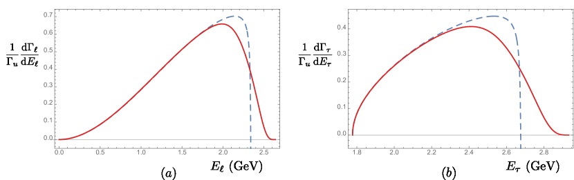
Figure 1: The $B\to X_{u}\ell\bar{\nu}$ lepton energy spectrum for (a) $\ell=e,\,\mu$ and (b) $\ell=\tau$ in the parton model (blue, dashed), and incorporating the leading order $b$-quark distribution function (red, solid).

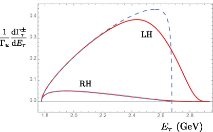
Figure 2: The $\tau$ energy dependence of its polarization in $B\to X_{u}\tau\bar{\nu}$ in the parton model (blue, dashed), and incorporating the leading order $b$-quark distribution function (red, solid).

The expression (28) is only valid in the region $\Delta\sim\Lambda_{\rm QCD}/m_{b}$; in order to have an expression which smoothly interpolates with the local OPE away from the endpoint, it is convenient instead to incorporate distribution function effects by redefining the $b$-quark mass $m_{b}\to m_{b}^{\prime}=m_{b}+k\cdot n$ [36, 28]. Writing $p_{b}^{\mu}=m_{b}^{\prime}v^{\mu}+k^{\prime\mu}$, where $k^{\prime\mu}=k^{\mu}-k\cdot n\,v^{\mu}$, the residual momentum $k^{\prime\mu}$ satisfies $k^{\prime}\cdot n=0$, and so the effects of nonzero $k\cdot n$ are automatically incorporated into the leading-order spectrum with this mass definition. The $\tau$ energy spectrum in the endpoint region may then be written as the convolution

$$\frac{{\rm d}\Gamma_{\tau}}{{\rm d}E_{\tau}}=2\int{\rm d}\omega\,\frac{1}{m_{b}}\frac{{\rm d}\Gamma_{\tau}}{{\rm d}y}(y^{\prime},\rho_{\tau}^{\prime})\,F(\omega)\,,$$ (30)

where we have defined the scaled variables

$$y^{\prime}\equiv\frac{2E_{\tau}}{m_{b}-\omega}\,,\qquad\rho_{\tau}^{\prime}\equiv\frac{m_{\tau}^{2}}{(m_{b}-\omega)^{2}}\,,$$ (31)

and ${\rm d}\Gamma/{\rm d}y$ is the parton level spectrum in Eq. (12). An analogous formula holds for the polarized spectrum Eq. (17). For simplicity, we have written the prefactor in Eq. (30) as $1/m_{b}$, not $1/(m_{b}-\omega)$, since the difference is higher order everywhere in the spectrum. In this form, Eq. (30) includes subleading terms suppressed by powers of $\Delta$ in the endpoint region, but which are leading order when $\Delta$ is not small, so are required to reproduce the local OPE away from the endpoint.

$F(k)$ has been extracted from the measured $B\to X_{s}\gamma$ spectra by the SIMBA collaboration [42]. At leading order in $\Lambda_{\rm QCD}/m_{b}$, it can be used to make predictions for $B\to X_{u}\ell\bar{\nu}$ decays. Figure 1 shows the $B\to X_{u}\ell\bar{\nu}$ lepton spectra for $\ell=e$ and $\ell=\tau$ in the parton model and including the effects of the $b$-quark distribution function. It is clear from this plot that the distribution function is indeed important in a greater fraction of the $\tau$ energy spectrum than in the massless lepton channels; the fraction of the lepton energy spectrum where the distribution function is important is enhanced by $(1-\rho_{\tau})/(1-\sqrt{}\rho_{\tau})^{2}\sim 2.2$. Figure 2 shows the $E_{\tau}$ spectra separately for left- and right-handed $\tau$ leptons in $B\to X_{u}\tau\bar{\nu}$. The average $\tau$ polarization, including order $\alpha_{s}$ and $\Lambda_{\rm QCD}^{2}/m_{b}^{2}$ corrections, is $2\tilde{\Gamma}/\Gamma=-0.77$.

IV Conclusions

We presented theoretical predictions for inclusive $B\to X_{u}\tau\bar{\nu}$ decay. We derived previously unknown results at order $\Lambda_{\rm QCD}^{2}/m_{b}^{2}$ and analytic expressions for the order $\alpha_{s}$ corrections for the $\tau$ energy spectrum and polarization. We also incorporated the effects of the $b$-quark light-cone distribution function to the case of nonzero lepton mass. Due to the suppressed kinematic range, the $b$-quark distribution function is more important in determining the lepton energy spectrum in $B\to X_{u}\tau\bar{\nu}$ than in $B\to X_{u}e\bar{\nu}$ decay.

It will probably take many ab^-1 of data at Belle II to have sensitivity to $B\to X_{u}\tau\bar{\nu}$. While it is clearly a challenging decay to measure, the rate according to Eqs. (1) and (I) is only about 3 times smaller than $B\to X_{u}e\bar{\nu}$, and about $|V_{cb}|^{2}/(3\,|V_{ub}|^{2})$ times smaller than $B\to X_{c}\tau\bar{\nu}$. One may, for example, try to utilize the fact that electrons or muons from the $\tau$ decay with maximal allowed energies correspond to the most energetic $\tau$ leptons. We hope that Belle II will be able to make measurements of this decay.