Could the Magnetic Star HD 135348 Possess a Rigidly Rotating Magnetosphere?

Abstract

We report the detection and characterization of a new magnetospheric star, HD 135348, based on photometric and spectropolarimetric observations. The TESS light curve of this star exhibited variations consistent with stars known to possess rigidly rotating magnetospheres (RRMs), so we obtained spectropolarimetric observations using the Robert Stobie Spectrograph (RSS) on the Southern African Large Telescope (SALT) at four different rotational phases. From these observations, we calculated the longitudinal magnetic field of the star $\langle B_{z}\rangle$, as well as the Alfvén and Kepler radii, and deduced that this star contains a centrifugal magnetosphere. However, an archival spectrum does not exhibit the characteristic “double-horned” emission profile for H$\alpha$ and the Brackett series that has been observed in many other RRM stars. This could be due to the insufficient rotational phase coverage of the available set of observations, as the spectra of these stars significantly vary with the star’s rotation. Our analysis underscores the use of TESS in photometrically identifying magnetic star candidates for spectropolarimetric follow-up using ground-based instruments. We are evaluating the implementation of a machine learning classifier to search for more examples of RRM stars in TESS data.

1 Introduction

The magnetic fields generated by hot, massive stars (types O, B, and A) have significant downstream effects. They can affect the surface rotation rates via magnetic braking (Weber & Davis, 1967; Ud-Doula et al., 2008), introduce chemical abundance inhomogeneities and peculiarities (Hunger & Groote, 1999), and confine the stellar wind in a magnetosphere (Friend & MacGregor, 1984; Babel & Montmerle, 1997; ud-Doula & Owocki, 2002). In such stars, the wind is driven along the field lines toward the magnetic equator – leading to a strong shock when the wind components of the two hemispheres collide. This heats the plasma to X-ray temperatures, a phenomenon that can be described by the magnetically confined wind shock model of Babel & Montmerle (1997).

Figure 3 of Petit et al. (2013) presents a classification scheme (the “magnetic confinement v/s rotation diagram”, henceforth MCRD) for stars that possess magnetospheres. This can be used to differentiate between two types of magnetospheres – centrifugal and dynamical; these classifications are based on two characteristic radii: the Alfvén radius, $R_{A}$, and the Keplerian co-rotation radius, $R_{K}$. Beyond $R_{A}$, the radial stellar wind forces the magnetic field lines to also become radial (see Altschuler & Newkirk 1969, and references therein).

A star has a dynamical magnetosphere when $R_{K}>R_{A}$; here, material confined in closed magnetic loops falls back onto the star’s surface on a dynamical timescale due to gravity (Sundqvist et al., 2012). On the other hand, a star has a centrifugal magnetosphere (CM) when $R_{A}>R_{K}$, i.e., material caught between $R_{A}$ and $R_{K}$ is supported against radial infall by a centrifugal force. This causes the plasma to build up, creating a relatively dense magnetosphere (Petit et al., 2013).

In some early B stars, the combination of rapid rotation and a strong magnetic field leads to the formation of a centrifugally supported magnetosphere with rotationally modulated hydrogen line emission. These stars, which can be accounted for by the rigidly rotating magnetosphere (RRM) model (Townsend & Owocki, 2005), are rare. The first one detected, $\sigma$ Ori E, was identified due to emission variability in hydrogen lines (specifically, H$\alpha$ and the Brackett series, i.e., transitions to the $n=4$ level of the H atom). The structure of the spectral features suggests that gas is trapped in magnetospheric clouds around the star, a conclusion derived from extensive modeling of its observational signatures by Townsend & Owocki (2005). Ten such stars have been identified as exhibiting a “double-horned” emission pattern at the H$\alpha$ wavelength (see the Introduction of Shultz et al. 2020, and references therein). These RRM stars are rather mysterious; their rotational velocities can approach breakup velocity, but their spin-down timescales via magnetic braking are significantly shorter than their estimated ages (Eikenberry et al., 2014).

The recent proliferation of large-scale, continuously observing space-based surveys has significantly increased the chance of identifying stars with detectable flux modulations potentially arising from a magnetosphere. Photometric missions such as the Kepler space telescope and the Transiting Exoplanet Survey Satellite (TESS ) have discovered several new classes of stars via their photometric modulation signatures; these techniques are easily extensible to the light curves of RRM stars (for models of these, see, e.g., Owocki et al. 2016; Krtička 2016). Thus, large-scale searches are underway that aim to identify and characterize rotational modulation profiles of stars observed by Kepler (see, e.g., Balona 2013; Balona et al. 2016) and TESS (see, e.g., David-Uraz et al. 2019; Sikora et al. 2019).

In this Letter, we present HD 135348, with spectral type B3V (from Hiltner et al. 1969), as a new magnetospheric B star identified through photometric observations obtained by TESS. We present spectropolarimetric observations of this star, along with a determination of its longitudinal magnetic field $\langle B_{z}\rangle$. Finally, we locate HD 135348 on the MCRD, and discuss this star in the context of other B stars with magnetospheres.

2 Observations

2.1 TESS Observations

HD 135348 (TIC 142505974) was observed by TESS during Sectors 11 and 38, which lasted from 2019 April 22 to 2019 May 21, and 2021 April 28 to 2021 May 26, respectively. During Sector 11, it was observed at 30-min cadence in the full-frame images (FFIs), while it was observed at 2-min cadence in Sector 38. The Sector 38 light curve is available in both SAP (simple aperture photometry) and PDCSAP (presearch data conditioning SAP) forms, which were generated by processing via the SPOC pipeline at the NASA Ames Research Center (Jenkins et al., 2016). We used the PDCSAP data for our analysis. We also used the eleanor package (Feinstein et al., 2019) to extract a light curve from the Sector 11 FFIs. The two light curves are shown in Figure 1.

Visual inspection indicates that the light curves in Figure 1 exhibit significant periodic variability. Taking a Discrete Fourier transform (see, e.g., Kurtz 1985), the results of which are presented in the bottom panel of Figure 1, we find a period of 2.0593 $\pm$ 0.0001 d. The additional peaks visible in the Fourier transform are harmonics of this fundamental frequency.

Figure 1: The top two panels show TESS light curves for HD 135348 from Sectors 11 and 38. The bottom panel contains a Discrete Fourier Transform of the Sector 38 data, showing a period of 2.0593 d. The data gap in the middle of the light curves is caused by the lack of observations during data downlink. Approximately 5% of the data points in the Sector 11 light curve were clipped. The removed points arise from scattered light entering the aperture; the deviations of these points from unity were found to be much greater than the semi-amplitude of the periodic flux variations ($\sim$5 ppt).

The light curve of HD 135348 looks similar to other magnetospheric stars observed by TESS , especially HD 23478, which is presented in the second panel of Figure 2. The third and fourth panels of Figure 2 show two other well-known RRM stars and highlight the diverse morphologies of the light curves of these stars. The fifth panel shows the light curve of HD 66765, the star located closest to HD 135348 on the MCRD (discussed further in Section 5); the bottom panel contains the light curve of a CM star, ALS 3694. Comparing the top 5 panels of this plot to the bottom one emphasizes the distinct morphologies of RRM and CM stars’ light curves, especially the large, noticeable dip(s) in flux exhibited by RRM stars; these features could enable us to photometrically identify such stars. This figure also contains the first published TESS light curves of RRM stars.

While the rotational period of HD 135348 is above average for RRM stars (e.g., HD 23478 has $P_{\rm rot}$ = 1.05 d; $\sigma$ Ori E has $P_{\rm rot}$ = 1.19 d), it is not out of the realm of possibility: CPD$-62^{\circ}2124$, mentioned in Shultz et al. (2020) as having H$\alpha$ emission consistent with the RRM model, has $P_{\rm rot}$ = 2.628 d (Hubrig et al., 2017).

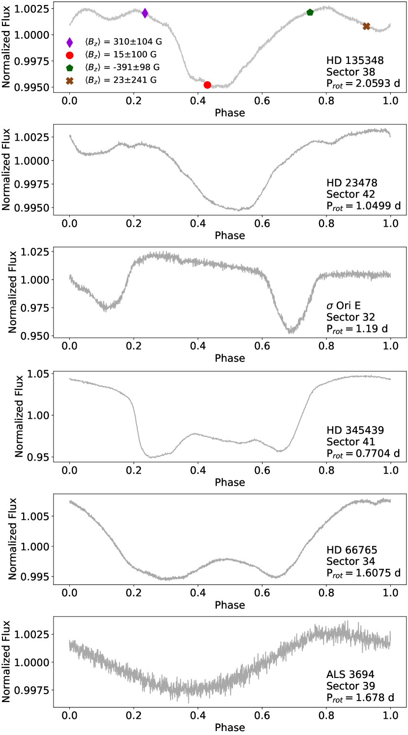
Figure 2: A comparison of binned, phase-folded TESS light curves for various magnetic stars with that of HD 135348 in the top panel. Its light curve most closely resembles that of the known RRM star HD 23478, shown in the second panel. The light curves of two other confirmed RRM stars, $\sigma$ Ori E and HD 345439, are shown in the third and fourth panels. The fifth panel shows the light curve of HD 66765, a star that shows H$\alpha$ in emission (a strong indicator that an RRM exists), and the bottom panel shows the light curve of a CM star, ALS 3694. The markers on the plot for HD 135348 represent the rotational phases at which the magnetic field measurements were made (see Section 2.2 and Table 1). We emphasize the significant differences in the light curve morphologies for CM and RRM stars. These light curves are binned to 0.002 units of phase. Note that the y-axis scales vary in each panel, in order to more clearly show the individual stars’ flux variations. The scatter visible in the light curve of ALS 3694 is likely not astrophysical in origin, and may simply be rms scatter.

2.2 SALT RSS Spectropolarimetry

The determination of magnetic fields in early B-type stars is usually based on measurements of the mean longitudinal magnetic field, i.e., of the line-of-sight field component averaged over the visible stellar hemisphere, using circularly polarized light. To search for a magnetic field in HD 135348, we obtained four low-resolution spectropolarimetric observations with the Robert Stobie Spectrograph (RSS; Burgh et al. 2003), mounted on the Southern African Large Telescope (SALT; Buckley et al. 2006). For more details about the RSS and how its data could be processed, we direct the reader to Brink et al. (2010), who discuss the first attempts at spectropolarimetric data reduction with SALT, and Potter et al. (2016), who discuss recent updates to the detector.

To probe the wavelength range of interest (4424 Å $<\lambda<$ 5090 Å), we used grating PG3000 at an angle of 46.625^∘ and a camera angle of 93.25^∘. With a 0.6 arcsec slitwidth, we achieved a spectral resolution of $R\sim 9600$. At each epoch, we took a continuous series of eight exposures using the standard readout mode. The quarter waveplate was oriented at a 45^∘ angle for exposures 1, 4, 5, and 8, and at 135^∘ for exposures 2, 3, 6, and 7. Each observation consisted of a 320 s integration (8 $\times$ 40 s) in order to achieve a S/N $\gtrsim$ 1000 per exposure.

We obtained observations of HD 135348 at four different epochs to sample different rotation phases (the zero point for the phases was chosen to coincide with the midpoint of the TESS observation, at BJD 2459347.88390; see Table 1 for the list of phases). This aimed to maximize the field detection probability and avoid missing the magnetic field due to a potentially unfavorable viewing angle at specific phases. The chemically peculiar A9VpSrCrEu star $\gamma$ Equ (HD 201601), with an extremely long rotation period of $>95.5$ yr (Bychkov et al., 2016; Savanov et al., 2018) and a well-characterized magnetic field, was used as a magnetic standard star. With $m_{\rm V}=4.7$, this bright star is frequently used to test and characterize instrumental polarimetric capabilities in both the Northern and Southern Hemispheres.

The first steps in the data reduction are standard processes for spectroscopic data; all raw frames were reduced using starlink software (Currie et al., 2014) to apply bias correction, cosmic ray masking, and flat fielding. The wavelength calibration was then carried out using CuAr arc lamp exposures obtained after the science frames. The wavelength solution for the O beam was applied to both the O and E beams in all observed spectra to ensure no drift in the wavelength solution.

The method to assess the presence of a magnetic field is very similar to that done using the European Southern Observatory (ESO) instruments FORS 1 and 2 in their spectropolarimetric mode. These techniques have been presented in many prior publications (see, e.g., Hubrig et al. 2004a, b, and references therein). We note that other works have made use of the polsalt reduction pipeline; however, this code cannot yet handle circular polarization data. The longitudinal magnetic field measurements are listed in Table 1.

Table 1: Longitudinal magnetic field values $\langle B_{z}\rangle$ obtained for $\gamma$ Equ and HD 135348 from RSS observations. The first column shows time of mid-exposure, followed by the signal-to-noise ratio ($S/N$) of the RSS Stokes $I$ spectra measured near 4480 Å. The measurements of $\langle B_{z}\rangle$ using the Monte Carlo bootstrapping test and the null spectra are presented in Columns 3 and 4. Finally, in Column 5, we indicate the rotational phase at which the measurement was taken. The zero point for the phases is BJD 2459347.88390, corresponding to the approximate midpoint of the TESS observation.

Date	$S/N$	$\left<B_{\rm z}\right>$		$\left<B_{\rm z}\right>_{N}$		Phase
(BJD-2400000)		(G)		(G)
$\gamma$ Equ
59437.43915	1349	$-$638$\pm$	36	$-$106$\pm$	34	N/A
HD 135348
59437.31835	1978	15$\pm$	100	$-$25$\pm$	109	0.430
59438.33863	1047	23$\pm$	241	8$\pm$	238	0.925
59448.27340	1740	$-$391$\pm$	98	$-$20$\pm$	105	0.749
59449.27366	1573	310$\pm$	104	41$\pm$	111	0.235

The mean longitudinal magnetic field $\langle B_{\rm z}\rangle=-638\pm 36$ G found for $\gamma$ Equ is consistent with recent measurements presented in Figure 1 of Hubrig et al. (2021), who observed this star using the high-resolution Potsdam Echelle Polarimetric and Spectroscopic Instrument (PEPSI), located at the Large Binocular Telescope. Specifically, this agrees with their measurement from 2019 May – $\langle B_{\rm z}\rangle=-663\pm 21$ G – and is generally consistent with the overall predicted variability of this star’s mean magnetic field $\langle B\rangle$ throughout time.

The strongest mean longitudinal magnetic field for HD 135348, $\langle B_{\rm z}\rangle=-391\pm 98$ G, is measured at a significance level of 4.0$\sigma$ at the rotation phase 0.749. After about half a rotation cycle, at phase 0.235, we measure a positive longitudinal field $\langle B_{\rm z}\rangle=310\pm 104$ G, at a significance level of 3.0$\sigma$. The detection of a magnetic field in HD 135348 makes this star a good candidate for long-term spectropolarimetric monitoring to fill in the gaps of its full magnetic phase curve.

3 Spectral variability

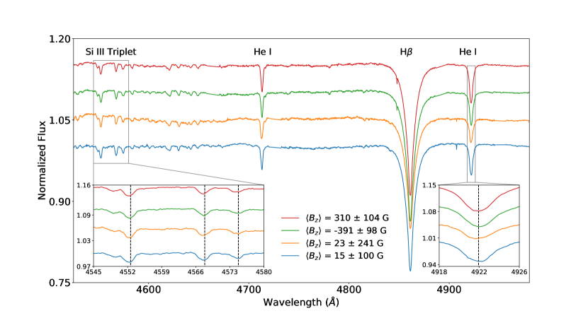
Figure 3: A plot of four Stokes $I$ spectra taken with the RSS over four different epochs with insets showing the variability of the line profiles of the Si iii triplet at 4552.62 Å, 4567.84 Å, and 4574.76 Å, along with the profiles of He i at 4921.93 Å. These wavelengths have been labeled with dotted vertical lines in both inset plots. Three of the four spectra have been offset for better visibility. We have labeled two other key spectral lines (another He i line, and also H$\beta$) visible in the plot.

RSS Stokes $I$ spectra showing the variability of different spectral lines are presented in Figure 3. To normalize each spectrum, we fit a fifth-order polynomial to the overall spectrum (masking out the largest and most relevant spectral lines), and then subtracted this fit from the raw data. The asymmetries in certain spectral line profiles, such as those of He i, arise from the inhomogeneous surface distribution of the corresponding elements, giving rise to chemical spots. As a result, the absorption varies with stellar rotation and manifests as a pronounced asymmetry in the corresponding spectral line (see, e.g., the bottom right inset plot in Figure 3, showing a large asymmetry in the He i line at 4922 Å).

While we attempted to calculate the radial velocity (RV) of the star, our accuracy was limited by the low resolution of the spectra and insufficient phase coverage. However, as shown in the inset in the bottom right of Figure 3, we observe significant variations in the He i line profile at the four observed phases, along with shifts in the RV. This behavior is expected for magnetic B type stars, especially those with surface He and Si spots. Archival RV values, from Wilson (1953) and Gontcharov (2006), indicate an average value of $-21\pm 3.5$ km s^-1. A crude calculation based on our observations suggests a mean RV of $\sim-$ 30 km s^-1 (with a large uncertainty). This value is in line with prior measurements; we plan to take further observations for a more precise estimate.

Finally, we used two different techniques to characterize the star’s rotational velocity and determine $v\,\sin\,i$. First, we used the mean profiles of the Si iii triplet lines observed at the four different epochs. This involved fitting Gaussians to these mean profiles to calculate their FWHM. This method yields an estimate for $v\,\sin\,i$ of 125 $\pm$ 9 km s^-1. To verify this value, we selected a sample of stars from Shultz et al. (2018) with similar spectral type (B2-B5) and magnetic field strength. We downloaded high-resolution spectra ($R\approx 65,000$) from the Echelle SpectroPolarimetric Device for the Observation of Stars at the Canada-France-Hawaii Telescope (Donati et al., 2006). These archival spectra were degraded to the resolution of the RSS by convolving them with a Gaussian profile. This enabled us to estimate that $v\,\sin\,i$ is $120\pm 10$ km s^-1. Our $v\,\sin\,i$ estimates are on the higher end for magnetic B stars, when compared to those in Table 1 of Petit et al. (2013). Consequently, we can conclude that this star is rapidly rotating, leading to a significantly smaller Keplerian co-rotation radius.

4 Estimating Stellar Parameters

The TESS Input Catalog (Stassun et al., 2019) does not have reliable stellar parameters for HD 135348, and the online SIMBAD catalog (Wenger et al., 2000) only contains information about the parallax, radial velocities, and inferred spectral type. As a result, we sought to derive a reliable estimate for these values to use for our calculations of magnetospheric properties, in Section 5.

This star is bright, with $m_{\rm V}=6.05$ and $T_{\rm mag}=6.184$ (Stassun et al., 2019). Typically, we would use an InfraRed Flux Method (IRFM) to calculate the temperature from a measured color index (see, e.g., Mucciarelli & Bellazzini 2020). However, the presence of chemical spots on B stars leads to significant flux redistribution from the far-UV region to the near-UV and visible regions of the spectrum (see, e.g., Section 5 in Krtička et al. 2013). This therefore precludes us from using broad-band color measurements, such as the $G-RP$ and $BP-G$ indices from Gaia. Moreover, many of the published IRFM coefficients are not valid for stars with $T_{\rm eff}\gtrsim 8000$ K. As a result, we use archival uvby$\beta$ colors (which are narrow-band) and estimate $T_{\rm eff}$ by interpolating within the grid of Moon & Dworetsky (1985).

The most recent uvby$\beta$ measurements are from Paunzen (2015). Two parameters, $\beta$ and $c_{1}$, are enough to estimate $T_{\rm eff}$; for HD 135348, $\beta=2.661\pm 0.006$, and $c_{1}=0.326\pm 0.01$. These measurements are consistent with archival data from Grønbech & Olsen (1977) and Hauck & Mermilliod (1998), but we add the caveat that such narrow-band color indices, while far more reliable, are still not immune from the photometric effects of chemical spots in B stars explored in Krtička et al. (2013) – emphasizing the importance of repeated, long-term measurements for these stars to obtain full phase coverage.

An estimate derived from the grid of Moon & Dworetsky (1985) yields $T_{\rm eff}\approx 16\,000\pm 1\,000$ K, assuming solar metallicity and a microturbulent velocity $\xi$ of 2.0 km s^-1 (many early- to intermediate-type B stars have $\xi\sim 1-10$ km s^-1 – see, e.g., Lefever et al. 2010). We use the Gaia parallax of $3.17\pm 0.07$ mas (Lindegren et al., 2021) and this star’s $m_{V}$ to calculate an absolute magnitude $M_{V}=-1.44\pm 0.05$. However, to convert this to a luminosity, we have to apply an appropriate bolometric correction as detailed in Bessell et al. (1998), assuming $log\,g=4.0$. This yields $M_{\rm V,bol}=-2.84\pm 0.05$, and a luminosity $L=1076\pm 50$ L_⊙. Then, we apply the Stefan-Boltzmann law to derive $R=4.27\pm 0.01$ R_⊙. Finally, we used the mass-luminosity relationship for intermediate-mass stars presented in Table 6 of Malkov (2007) to obtain $M_{*}=5.66_{-0.08}^{+0.06}$ M_⊙. This yields $\log\,g=3.93\pm 0.01$.

Using our derived parameters and the tables of Pecaut & Mamajek (2013), we identify this star’s spectral type as B2.5-4V. This agrees with the spectral type of B3V in Hiltner et al. (1969). We additionally emphasize that interstellar reddening does not significantly affect our color estimates, as the extinction coefficient $A_{G}=0.06$. Our inferred spectral type agrees with those of other known RRM stars, which are all early- to intermediate-B stars.

5 The Magnetosphere of HD 135348

5.1 Is the Magnetosphere Centrifugal or Dynamical?

First, we estimate $R_{A}$ and $R_{K}$. The former is derived from the magnetic wind confinement parameter $\eta_{*}$:

$$\eta_{*}=\frac{B_{\rm eq}^{2}R_{*}^{2}}{\dot{M}_{B=0}V_{\infty}}.$$ (1)

We can use the definitions and equations from Petit et al. (2013) to calculate $\eta_{*}$. Firstly, $B_{\rm eq}\equiv B_{d}/2$, where $B_{d}$ is thrice the largest longitudinal magnetic field measurement (in our case, $\sim$1.2 kG). Also, $\dot{M}_{B=0}$ and $V_{\infty}$ are the fiducial mass-loss rate and the “terminal speed” that the stellar wind would have with no magnetic field:

$$\dot{M}_{B=0}=0.551\frac{L_{*}}{c^{2}}\left(\frac{1000\Gamma_{e}}{1-\Gamma_{e}}\right)^{0.818}$$ (2)

$$V_{\rm esc}\equiv\left(\frac{2GM_{*}\left(1-\Gamma_{e}\right)}{R_{*}}\right)^{1/2}.$$ (3)

Here, $\Gamma_{e}=\kappa_{e}L_{*}/4\pi GM_{*}c$ is the Eddington parameter for the electron scattering opacity, $\kappa_{e}$. We thus obtain $\eta_{*}=8.78\pm 2.99\times 10^{3}$. We substitute $\eta_{*}$ to find $R_{A}$:

$$\frac{R_{A}}{R_{*}}\approx 0.3+\left(\eta_{*}+0.25\right)^{1/4}.$$ (4)

This yields $R_{A}\approx 9.98\pm 0.82$ R_∗.

We find $R_{K}$, given by

$$R_{K}\equiv\left(\frac{GM}{\omega^{2}}\right)^{\frac{1}{3}},$$ (5)

to be $10.86\pm 0.02$ R_⊙. This implies that $R_{K}/R_{*}\sim 2.84$.

With estimates for $R_{A}$ and $R_{K}$, we can see that $R_{A}>R_{K}$ and thus place HD 135348 on the MCRD in the region containing stars possessing a centrifugal magnetosphere. Its closest neighbor on the MCRD is HD 66765, which was found to exhibit (relatively weak) H$\alpha$ emission lines (see Figure B1 in Shultz et al. 2020). However, the fact that this star has both H$\alpha$ emission and a light curve reminiscent of other RRM stars (see Figure 2) strongly suggests that this star also possesses an RRM. Additionally, Shultz et al. (2020) claim that the RRM model can adequately explain the observed H$\alpha$ emission of stars in this region of the MCRD, implying that such a model can explain our photometric observations of HD 135348.

Indeed, all that is needed for an RRM to exist is that $R_{A}>R_{K}$, which we have proven for HD 135348. Eikenberry et al. (2014) state that RRMs are more likely to occur in stars with magnetic fields $>10$ kG, but are not improbable in stars with dipole magnetic fields of $\sim 1$ kG – such as HD 135348. We thus sought to directly compare key spectral features of RRM stars to archival spectra of HD 135348 to evaluate this claim.

5.2 Comparison to Known RRM Stars

We used archival observations from the XSHOOTER and UVES spectrographs (Vernet et al., 2011; Dekker et al., 2000) on the Very Large Telescope (VLT). These spectrographs enable us to investigate two regions that we could not study with our chosen RSS configuration: H$\alpha$ ($\lambda=6562.3$ Å), and the Brackett series, for $n\gtrsim 10$. The XSHOOTER spectrum for HD 135348 ($R\sim 5040$, S/N $\sim 260$) was obtained on 2013 March 2, with an exposure time of 5 s, and spans 5340 to 21000 Å. We compared this to observations of HR 5907, a known RRM star, that were taken using UVES on 2010 April 13 and XSHOOTER on 2014 April 29. For all spectra, we used the processed version from the ESO Science Portal.

In contrast to typical RRM stars, the archival spectrum of HD 135348 does not show an emission profile at H$\alpha$, or throughout the Brackett series; this, however, does not exclude the possibility of emission at different rotation phases. Known RRM stars, such as HR 5907, exhibit a characteristic “double-horned” emission-line profile throughout the Brackett series, especially for $n>10$ (see Fig. 1 in Eikenberry et al. 2014). In Figure 4, we show a comparison of the Brackett series for HR 5907 and HD 135348; the archival spectrum shows only absorption features for the latter star.

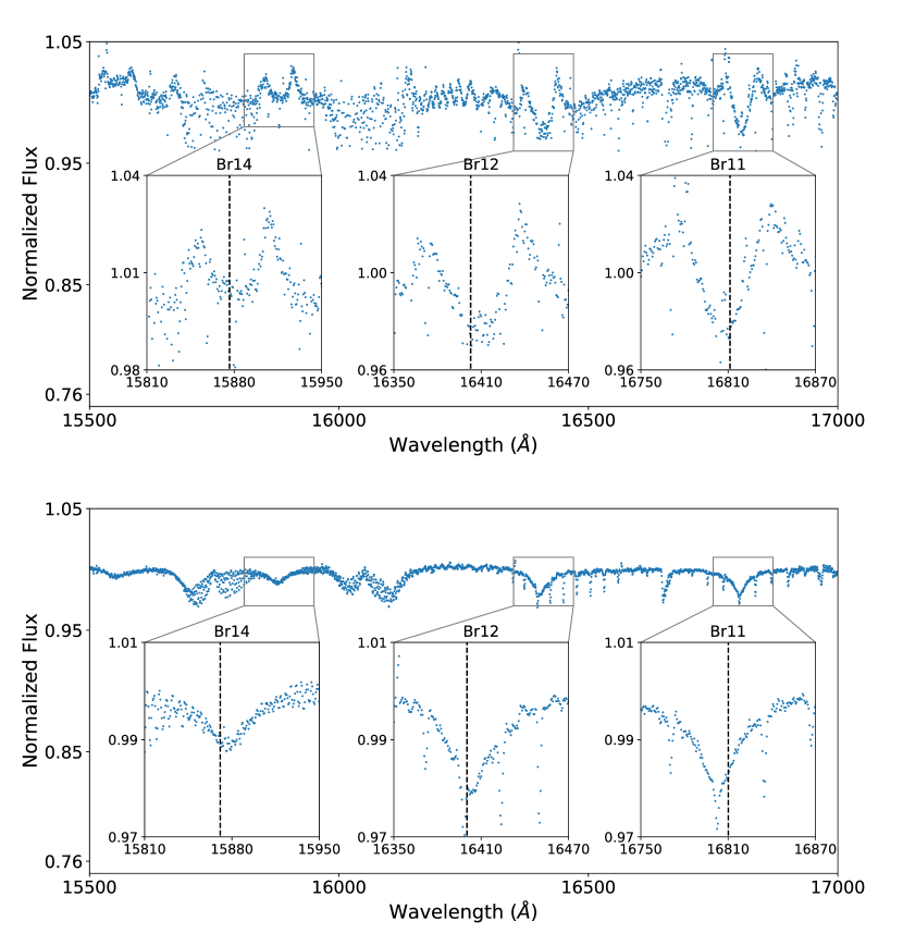
Figure 4: Archival XSHOOTER spectra showing “double-horned” Brackett line emission for HR 5907 (top panel), compared with the lack of a similar profile in HD 135348 (bottom panel). A similar plot of the Brackett series, albeit for HD 23478 and HD 345439, can be found in figure 1 of Eikenberry et al. (2014). The dotted vertical lines mark the wavelengths of the corresponding Brackett series line (Br14: 15876.3 Å, Br12: 16402.8 Å, Br11: 16802 Å).

Some other RRM stars exhibit a similar double-horned symmetric profile at the core of the H$\alpha$ line, but this is not universal across known RRM stars (e.g., there is a pronounced asymmetry in the “horns” of the line profile in the spectrum of HD 345439 – see the inset in Fig. 3 of Eikenberry et al. 2014). In a number of RRM stars, the H$\alpha$ emission is also highly variable and could disappear at some rotational phases. Visual inspection of the H$\alpha$ region of the spectra for both HR 5907 and HD 135348 revealed a “double-horned” profile for HR 5907, but only an absorption feature in the spectrum of HD 135348. As a result, we claim that this is a CM star, but cannot definitively conclude whether this is an RRM star, due to the insufficient phase coverage of available spectroscopic observations.

Shultz et al. (2020) postulate that RRMs may be a subclass of CM stars, albeit with with a favorable viewing angle. The stellar wind plasma accumulates in a torus around the star’s magnetic equatorial plane. When the clouds of plasma transit the star, we observe H$\alpha$ absorption; in stars where the centrifugal magnetosphere is seen face-on, the emission of an RRM peaks at $R_{K}$, which leads to the characteristic double-horned profile. On the other hand, Owocki et al. (2020) suggest that a lack of emission around H$\alpha$, which is commonly observed in stars with spectral type later than $\sim$B6 ($T_{\rm eff}\lesssim 16$ kK and L $\lesssim 800$ L_⊙), may arise from leakage that prevents filling of the CM to the level needed for H$\alpha$ emission (because of a lower $\dot{M}$) or the predominance of a metal-ion driven wind, which would lack the hydrogen needed for emission. HD 135348, which we infer to be an intermediate B star in Section 4, could possess such an underdense centrifugal magnetosphere – a potential explanation for the lack of observed hydrogen emission.

The major implication of our study is the fact that we can potentially photometrically identify RRM candidates from large-scale sky surveys. With the vast amounts of data we will obtain as large sky surveys (such as the Vera Rubin Observatory) come online, and space-based surveys such as TESS continue observing large parts of the sky, we could train a machine learning algorithm to search for characteristic features of RRM light curves using the model described in Townsend (2008).

6 Conclusions

In this Letter, we use TESS data and spectropolarimetric observations to characterize a magnetic B star, HD 135348. Our observations and calculations allow us to deduce that this star possesses a centrifugal magnetosphere and could potentially be an RRM star. However, we cannot make a conclusive determination about the latter point due to the small number of magnetic field measurements, which neither provide full rotational phase coverage nor enable us to deduce the field strength and its geometry. Future work will entail obtaining additional spectropolarimetric observations to construct this star’s full magnetic phase curve, enabling us to either verify or discount the presence of an RRM.

We note that this is the first publication to present TESS photometry of RRM stars. TESS’s short-cadence continuous observations have enabled us to precisely constrain stellar rotation rates. Further TESS data on any RRM star can also constrain any variability in the light curve between cycles, as these stars have comparatively short rotational periods ($\lesssim 2.5$ d), and a single TESS observing sector covers several rotation cycles. We are also developing a machine learning classifier to identify high-likelihood RRM star candidates in TESS data for spectropolarimetric follow-up.

Data Availability

Data from the TESS Mission is available on the Barbara A. Mikulski Archive for Space Telescopes (mast.stsci.edu). Resources supporting this work were provided by the NASA High-End Computing (HEC) Program through the NASA Advanced Supercomputing (NAS) Division at Ames Research Center for the production of SPOC data products. Data from SALT observations are made available to the public after a 6-month proprietary period. Both raw and processed spectra from XSHOOTER and UVES can be downloaded through the ESO Science Portal (https://archive.eso.org/scienceportal/). The ESPaDOnS data used in this article are available in the CFHT Science Archive at https://www.cadc-ccda.hia-iha.nrc-cnrc.gc.ca/en/cfht/.

References

- Altschuler & Newkirk (1969) Altschuler, M. D., & Newkirk, G. 1969, Sol. Phys., 9, 131, doi: 10.1007/BF00145734
- Astropy Collaboration et al. (2013) Astropy Collaboration, Robitaille, T. P., Tollerud, E. J., et al. 2013, A&A, 558, A33, doi: 10.1051/0004-6361/201322068
- Astropy Collaboration et al. (2018) Astropy Collaboration, Price-Whelan, A. M., Sipőcz, B. M., et al. 2018, AJ, 156, 123, doi: 10.3847/1538-3881/aabc4f
- Babel & Montmerle (1997) Babel, J., & Montmerle, T. 1997, A&A, 323, 121
- Balona (2013) Balona, L. A. 2013, in Stellar Pulsations: Impact of New Instrumentation and New Insights, ed. J. C. Suárez, R. Garrido, L. A. Balona, & J. Christensen-Dalsgaard, Vol. 31, 247, doi: 10.1007/978-3-642-29630-7_45
- Balona et al. (2016) Balona, L. A., Švanda, M., & Karlický, M. 2016, MNRAS, 463, 1740, doi: 10.1093/mnras/stw2109
- Bessell et al. (1998) Bessell, M. S., Castelli, F., & Plez, B. 1998, A&A, 333, 231
- Brink et al. (2010) Brink, J. D., Buckley, D. A. H., Nordsieck, K. H., & Potter, S. B. 2010, in Society of Photo-Optical Instrumentation Engineers (SPIE) Conference Series, Vol. 7735, Ground-based and Airborne Instrumentation for Astronomy III, ed. I. S. McLean, S. K. Ramsay, & H. Takami, 773517, doi: 10.1117/12.856932
- Buckley et al. (2006) Buckley, D. A. H., Swart, G. P., & Meiring, J. G. 2006, in Society of Photo-Optical Instrumentation Engineers (SPIE) Conference Series, Vol. 6267, Society of Photo-Optical Instrumentation Engineers (SPIE) Conference Series, ed. L. M. Stepp, 62670Z, doi: 10.1117/12.673750
- Burgh et al. (2003) Burgh, E. B., Nordsieck, K. H., Kobulnicky, H. A., et al. 2003, in Society of Photo-Optical Instrumentation Engineers (SPIE) Conference Series, Vol. 4841, Instrument Design and Performance for Optical/Infrared Ground-based Telescopes, ed. M. Iye & A. F. M. Moorwood, 1463–1471, doi: 10.1117/12.460312
- Bychkov et al. (2016) Bychkov, V. D., Bychkova, L. V., & Madej, J. 2016, MNRAS, 455, 2567, doi: 10.1093/mnras/stv2416
- Currie et al. (2014) Currie, M. J., Berry, D. S., Jenness, T., et al. 2014, in Astronomical Society of the Pacific Conference Series, Vol. 485, Astronomical Data Analysis Software and Systems XXIII, ed. N. Manset & P. Forshay, 391
- David-Uraz et al. (2019) David-Uraz, A., Neiner, C., Sikora, J., et al. 2019, MNRAS, 487, 304, doi: 10.1093/mnras/stz1181
- Dekker et al. (2000) Dekker, H., D’Odorico, S., Kaufer, A., Delabre, B., & Kotzlowski, H. 2000, in Society of Photo-Optical Instrumentation Engineers (SPIE) Conference Series, Vol. 4008, Optical and IR Telescope Instrumentation and Detectors, ed. M. Iye & A. F. Moorwood, 534–545, doi: 10.1117/12.395512
- Donati et al. (2006) Donati, J. F., Catala, C., Landstreet, J. D., & Petit, P. 2006, in Astronomical Society of the Pacific Conference Series, Vol. 358, Solar Polarization 4, ed. R. Casini & B. W. Lites, 362
- Drimmel et al. (2019) Drimmel, R., Bucciarelli, B., & Inno, L. 2019, Research Notes of the AAS, 3, 79, doi: 10.3847/2515-5172/ab2632
- Eikenberry et al. (2014) Eikenberry, S. S., Chojnowski, S. D., Wisniewski, J., et al. 2014, ApJ, 784, L30, doi: 10.1088/2041-8205/784/2/L30
- Feinstein et al. (2019) Feinstein, A. D., Montet, B. T., Foreman-Mackey, D., et al. 2019, eleanor: Extracted and systematics-corrected light curves for TESS-observed stars. http://ascl.net/1904.022
- Friend & MacGregor (1984) Friend, D. B., & MacGregor, K. B. 1984, ApJ, 282, 591, doi: 10.1086/162238
- Gaia Collaboration et al. (2016) Gaia Collaboration, Prusti, T., de Bruijne, J. H. J., et al. 2016, A&A, 595, A1, doi: 10.1051/0004-6361/201629272
- Gaia Collaboration et al. (2021) Gaia Collaboration, Brown, A. G. A., Vallenari, A., et al. 2021, A&A, 649, A1, doi: 10.1051/0004-6361/202039657
- Gontcharov (2006) Gontcharov, G. A. 2006, Astronomy Letters, 32, 759, doi: 10.1134/S1063773706110065
- Grønbech & Olsen (1977) Grønbech, B., & Olsen, E. H. 1977, A&AS, 27, 443
- Harris et al. (2020) Harris, C. R., Millman, K. J., van der Walt, S. J., et al. 2020, Nature, 585, 357, doi: 10.1038/s41586-020-2649-2
- Hauck & Mermilliod (1998) Hauck, B., & Mermilliod, M. 1998, A&AS, 129, 431, doi: 10.1051/aas:1998195
- Hiltner et al. (1969) Hiltner, W. A., Garrison, R. F., & Schild, R. E. 1969, ApJ, 157, 313, doi: 10.1086/150069
- Hubrig et al. (2021) Hubrig, S., Järvinen, S. P., Ilyin, I., Strassmeier, K. G., & Schöller, M. 2021, MNRAS, doi: 10.1093/mnrasl/slab101
- Hubrig et al. (2004a) Hubrig, S., Kurtz, D. W., Bagnulo, S., et al. 2004a, A&A, 415, 661, doi: 10.1051/0004-6361:20031380
- Hubrig et al. (2017) Hubrig, S., Mikulášek, Z., Kholtygin, A. F., et al. 2017, MNRAS, 472, 400, doi: 10.1093/mnras/stx1994
- Hubrig et al. (2004b) Hubrig, S., Szeifert, T., Schöller, M., Mathys, G., & Kurtz, D. W. 2004b, A&A, 415, 685, doi: 10.1051/0004-6361:20031486
- Hunger & Groote (1999) Hunger, K., & Groote, D. 1999, A&A, 351, 554
- Hunter (2007) Hunter, J. D. 2007, Computing in Science & Engineering, 9, 90, doi: 10.1109/MCSE.2007.55
- Jenkins et al. (2016) Jenkins, J. M., Twicken, J. D., McCauliff, S., et al. 2016, in Proc. SPIE, Vol. 9913, Software and Cyberinfrastructure for Astronomy IV, 99133E, doi: 10.1117/12.2233418
- Krtička (2016) Krtička, J. 2016, A&A, 594, A75, doi: 10.1051/0004-6361/201629222
- Krtička et al. (2013) Krtička, J., Janík, J., Marková, H., et al. 2013, A&A, 556, A18, doi: 10.1051/0004-6361/201221018
- Kupka et al. (1999) Kupka, F., Piskunov, N., Ryabchikova, T. A., Stempels, H. C., & Weiss, W. W. 1999, A&AS, 138, 119, doi: 10.1051/aas:1999267
- Kurtz (1985) Kurtz, D. W. 1985, MNRAS, 213, 773, doi: 10.1093/mnras/213.4.773
- Lefever et al. (2010) Lefever, K., Puls, J., Morel, T., et al. 2010, A&A, 515, A74, doi: 10.1051/0004-6361/200911956
- Lindegren et al. (2021) Lindegren, L., Klioner, S. A., Hernández, J., et al. 2021, A&A, 649, A2, doi: 10.1051/0004-6361/202039709
- Malkov (2007) Malkov, O. Y. 2007, MNRAS, 382, 1073, doi: 10.1111/j.1365-2966.2007.12086.x
- Moon & Dworetsky (1985) Moon, T. T., & Dworetsky, M. M. 1985, MNRAS, 217, 305, doi: 10.1093/mnras/217.2.305
- Mucciarelli & Bellazzini (2020) Mucciarelli, A., & Bellazzini, M. 2020, Research Notes of the American Astronomical Society, 4, 52, doi: 10.3847/2515-5172/ab8820
- Owocki et al. (2020) Owocki, S. P., Shultz, M. E., ud-Doula, A., et al. 2020, MNRAS, 499, 5366, doi: 10.1093/mnras/staa2325
- Owocki et al. (2016) Owocki, S. P., ud-Doula, A., Sundqvist, J. O., et al. 2016, MNRAS, 462, 3830, doi: 10.1093/mnras/stw1894
- pandas development team (2020) pandas development team, T. 2020, pandas-dev/pandas: Pandas, latest, Zenodo, doi: 10.5281/zenodo.3509134
- Paunzen (2015) Paunzen, E. 2015, A&A, 580, A23, doi: 10.1051/0004-6361/201526413
- Pecaut & Mamajek (2013) Pecaut, M. J., & Mamajek, E. E. 2013, ApJS, 208, 9, doi: 10.1088/0067-0049/208/1/9
- Petit et al. (2013) Petit, V., Owocki, S. P., Wade, G. A., et al. 2013, MNRAS, 429, 398, doi: 10.1093/mnras/sts344
- Potter et al. (2016) Potter, S. B., Nordsieck, K., Romero-Colmenero, E., et al. 2016, in Society of Photo-Optical Instrumentation Engineers (SPIE) Conference Series, Vol. 9908, Ground-based and Airborne Instrumentation for Astronomy VI, ed. C. J. Evans, L. Simard, & H. Takami, 99082K, doi: 10.1117/12.2232391
- Savanov et al. (2018) Savanov, I. S., Romanyuk, I. I., & Dmitrienko, E. S. 2018, Astrophysical Bulletin, 73, 463, doi: 10.1134/S1990341318040089
- Shultz et al. (2018) Shultz, M. E., Wade, G. A., Rivinius, T., et al. 2018, MNRAS, 475, 5144, doi: 10.1093/mnras/sty103
- Shultz et al. (2020) Shultz, M. E., Owocki, S., Rivinius, T., et al. 2020, MNRAS, 499, 5379, doi: 10.1093/mnras/staa3102
- Sikora et al. (2019) Sikora, J., David-Uraz, A., Chowdhury, S., et al. 2019, MNRAS, 487, 4695, doi: 10.1093/mnras/stz1581
- Stassun et al. (2019) Stassun, K. G., Oelkers, R. J., Paegert, M., et al. 2019, AJ, 158, 138, doi: 10.3847/1538-3881/ab3467
- Sundqvist et al. (2012) Sundqvist, J. O., ud-Doula, A., Owocki, S. P., et al. 2012, MNRAS, 423, L21, doi: 10.1111/j.1745-3933.2012.01248.x
- Townsend (2008) Townsend, R. H. D. 2008, MNRAS, 389, 559, doi: 10.1111/j.1365-2966.2008.13462.x
- Townsend & Owocki (2005) Townsend, R. H. D., & Owocki, S. P. 2005, MNRAS, 357, 251, doi: 10.1111/j.1365-2966.2005.08642.x
- ud-Doula & Owocki (2002) ud-Doula, A., & Owocki, S. P. 2002, ApJ, 576, 413, doi: 10.1086/341543
- Ud-Doula et al. (2008) Ud-Doula, A., Owocki, S. P., & Townsend, R. H. D. 2008, MNRAS, 385, 97, doi: 10.1111/j.1365-2966.2008.12840.x
- Vernet et al. (2011) Vernet, J., Dekker, H., D’Odorico, S., et al. 2011, A&A, 536, A105, doi: 10.1051/0004-6361/201117752
- Virtanen et al. (2020) Virtanen, P., Gommers, R., Oliphant, T. E., et al. 2020, Nature Methods, 17, 261, doi: 10.1038/s41592-019-0686-2
- Weber & Davis (1967) Weber, E. J., & Davis, Leverett, J. 1967, ApJ, 148, 217, doi: 10.1086/149138
- Wenger et al. (2000) Wenger, M., Ochsenbein, F., Egret, D., et al. 2000, Astronomy and Astrophysics Supplement Series, 143, 9, doi: 10.1051/aas:2000332
- Wes McKinney (2010) Wes McKinney. 2010, in Proceedings of the 9th Python in Science Conference, ed. Stéfan van der Walt & Jarrod Millman, 56 – 61, doi: 10.25080/Majora-92bf1922-00a
- Wilson (1953) Wilson, R. E. 1953, Carnegie Institute Washington D.C. Publication, 0