On the quenching of star formation in observed and simulated central galaxies: Evidence for the role of integrated AGN feedback

Abstract

In this paper we investigate how massive central galaxies cease their star formation by comparing theoretical predictions from cosmological simulations: EAGLE, Illustris and IllustrisTNG with observations of the local Universe from the Sloan Digital Sky Survey (SDSS). Our machine learning (ML) classification reveals supermassive black hole mass (${M_{\rm BH}}$) as the most predictive parameter in determining whether a galaxy is star forming or quenched at redshift $z=0$ in all three simulations. This predicted consequence of active galactic nucleus (AGN) quenching is reflected in the observations, where it is true for a range of indirect estimates of ${M_{\rm BH}}$ via proxies as well as its dynamical measurements. Our partial correlation analysis shows that other galactic parameters lose their strong association with quiescence, once their correlations with ${M_{\rm BH}}$ are accounted for. In simulations we demonstrate that it is the integrated power output of the AGN, rather than its instantaneous activity, which causes galaxies to quench. Finally, we analyse the change in molecular gas content of galaxies from star forming to passive populations. We find that both gas fractions ($f_{\rm gas}$) and star formation efficiencies (SFEs) decrease upon transition to quiescence in the observations but SFE is more predictive than $f_{\rm gas}$ in the ML passive/star-forming classification. These trends in the SDSS are most closely recovered in IllustrisTNG and are in direct contrast with the predictions made by Illustris. We conclude that a viable AGN feedback prescription can be achieved by a combination of preventative feedback and turbulence injection which together quench star formation in central galaxies.

1 Introduction

The launch of large surveys like the Sloan Digital Sky Survey (SDSS) (York et al., 2000), revealed that local galaxies reside either in the ‘blue cloud’ or the ‘red sequence’ in the colour-magnitude diagram (e.g. Strateva et al., 2001; Baldry et al., 2004; Wyder et al., 2007) and that this division persists to as far back as redshift $z\sim 3$ (e.g. Giallongo et al., 2005; Brammer et al., 2009; Willmer et al., 2006). The distribution in galactic colour, however, reflects a more fundamental bimodal distribution in the specific star formation rate (sSFR, star formation rate per unit stellar mass) (e.g. Kauffmann et al., 2003; Santini et al., 2009), owing to significantly different optical signatures between young and old stellar populations (e.g. Bruzual & Charlot, 2003; Maraston & Strömbäck, 2011). When observed across cosmic time, the mass density in the red, passive population increases in size, while it remains roughly constant in the star forming cloud (e.g. Bell et al., 2004; Faber et al., 2007). This observation is generally interpreted as a change in the object membership between the two populations as a consequence of star formation slowing down. As a result, quenching is at large defined as the process of galaxy transition between the blue cloud and the red sequence over time. For the purpose of our research, however, quenching refers specifically to the change in location in the stellar mass (${M_{\ast}}$) – star formation rate (SFR) plane during which galaxies fall off the star forming Main Sequence (MS, Noeske et al. 2007; Brinchmann et al. 2004) to join the ‘passive’ population with low sSFRs.

Quenching has been shown to correlate well with galaxy stellar mass (e.g. Baldry et al., 2006; Peng et al., 2010; Liu et al., 2019; Bluck et al., 2019), halo mass (e.g. Woo et al., 2013; Wang et al., 2018), morphology (e.g. Cameron & Driver 2009; Cameron et al. 2009; Bell et al. 2012; Bluck et al. 2014; Omand et al. 2014), the angular momentum of inflowing gas (i.e. angular momentum quenching, Peng & Renzini 2020, Renzini 2020), stellar kinematics (Wang et al., 2020), central velocity dispersion (e.g. Wake et al. 2012; Teimoorinia et al. 2016; Bluck et al. 2016; Bluck et al. 2019; Bluck et al. 2020a; Bluck et al. 2020b) and, more recently, with dynamically measured supermassive black hole mass (e.g. Terrazas et al., 2016, 2017; Martín-Navarro et al., 2018). In the case of satellite galaxies, an additional connection between environment and quiescence was revealed, where the star forming state of an object depends on local overdensity and its location within the parent dark matter halo (e.g. van den Bosch et al., 2008; Peng et al., 2012; Woo et al., 2013; Bluck et al., 2016; Liu et al., 2019). In this study we choose to focus on central galaxies only, in order to investigate the intrinsic quenching mechanisms, unaffected by the galactic environment.

X-ray observations of galaxy clusters brought a crucial understanding of the macrophysics of quenching, showing that the bulk of baryonic matter associated with massive elliptical galaxies resides in their surrounding haloes in a form of hot, ionised gas (e.g. Paolillo et al., 2002; Fukazawa et al., 2006; Humphrey et al., 2011). The main cooling channel for this plasma is via the free-free interaction and predicts much higher cold gas mass accretion rates onto the galaxies than found in the observations (see McNamara & Nulsen, 2007, for a review). Therefore, it is apparent that one fundamental operational mechanism of quenching is to provide enough heat to offset cooling and keep galactic halos hot. This way, a substantial reservoir of gas is prevented from collapsing onto a galaxy and not allowed to deliver fuel for active star formation.

The microphysics of how the temperature of the haloes is kept high, however, remains an open question. One proposed solution is the shock-heating of gas as it falls through deep halo potential wells as suggested by Dekel & Birnboim (2006) and observationally supported by e.g. Woo et al. (2013), Tal et al. (2014) and Wang et al. (2018). Alternatively, accretion onto supermassive black holes in active galactic nuclei (AGN) is a strong candidate for a heating source, since it can generate enough energy to offset high cooling rates in galaxy clusters (e.g. Silk & Rees, 1998; Binney, 2004; Scannapieco & Oh, 2004). In fact, modern cosmological simulations can only successfully shut down star formation in massive galaxies using some form of AGN feedback, as other processes like supernova explosions are not able to prevent galaxies from constantly forming stars at redshift $z=0$ (e.g Bower et al., 2006; McCarthy et al., 2011; Dubois et al., 2016; Weinberger et al., 2017).

The ongoing AGN debate revolves around the exact energy deposition mechanism within the galactic halo – whether it is achieved through violent outflows of gas in the high accretion ‘quasar mode’ (e.g. Hopkins et al., 2008; Hopkins & Elvis, 2010; Villar-Martín et al., 2011; Maiolino et al., 2012) or rather through slow and steady energy injection in the low accretion ‘preventative’ feedback mode (e.g. McNamara et al., 2000; Bîrzan et al., 2004; Fabian, 2012; Hlavacek-Larrondo et al., 2012; Hlavacek-Larrondo et al., 2015). From an observational perspective, there exists evidence in favour of both heating avenues, however the exact mechanism of coupling the AGN power to the halo gas is not well determined yet (see Werner et al., 2019, for a review).

More recently, a breakthrough in our understanding of quenching came along with the first integrated and spatially resolved surveys of directly measured molecular gas content in galaxies (Bolatto et al., 2017; Saintonge et al., 2017, 2018; Tacconi et al., 2018; Sorai et al., 2019; Aravena et al., 2019; Lin et al., 2020). By translating CO line luminosities to ${\rm H}_{2}$ masses, multiple authors found a significant variation in gas fractions ($f_{\rm gas}=M_{\rm H2}/M_{\ast}$) across the $M_{\ast}-{\rm SFR}$ plane with galaxies below the MS showing significantly lower $f_{\rm gas}$ than their MS counterparts (e.g. Genzel et al. 2015; Lin et al. 2017; Saintonge et al. 2017; Belli et al. 2021; Ellison et al. 2021; Dou et al. 2021a; Dou et al. 2021b). Even more interestingly, a significant fraction of these studies additionally found decreasing star formation efficiencies ($\rm{SFE=SFR/}M_{\rm gas}$, the inverse of gas depletion time $t_{\rm dep}$), away from the Main Sequence with the magnitude of the decrease in SFE exceeding that of $f_{\rm gas}$ (e.g. Tacconi et al., 2018; Lin et al., 2020; Colombo et al., 2020; Ellison et al., 2020; Dou et al., 2021a, b). In Piotrowska et al. (2020), we used the reddening of optical SDSS spectra to estimate the in-fibre molecular gas masses for $\sim 60\,000$ galaxies and confirmed the above trends in a significantly larger sample of local galaxies. This combined observational evidence suggests a new macrophysical property of a successful quenching paradigm – galaxies do not cease their star formation by solely depleting their gas reservoirs. Instead, it is the combined effect of the lack of star forming fuel and its reduced potential for gravitational collapse, which work in tandem to drive massive local galaxies towards quiescence.

Much like in the case of heating in the galactic haloes, the microphysics of $f_{\rm gas}$ reduction offers room for debate. On the one hand, low gas fractions can stem from molecular gas consumption via star formation, in the absence of fresh gas supply from the constantly heated surrounding halo. However, one can easily imagine a scenario in which cold gas is also removed from the galaxy, owing to momentum kicks from supernova explosions (e.g. Kay et al., 2002; Marri & White, 2003) or quasar activity (e.g. Maiolino et al., 2012; Harrison et al., 2014; Zakamska & Greene, 2014) or both (e.g. Fluetsch et al., 2019). As shown in a body of theoretical work (e.g. Springel & Hernquist, 2003; Hopkins et al., 2011; Pontzen et al., 2017; Henriques et al., 2019) supernova feedback is only likely to be relevant in low-mass galaxies, where gravitational potential wells are shallow enough to prevent gas re-accretion via galactic fountains. The picture is less clear about AGN – although quasar outflows have been found to carry significant masses of gas in both the ionised (e.g. Carniani et al., 2015; Rupke et al., 2017) and molecular phases (e.g. Feruglio et al., 2010; Veilleux et al., 2013; Fluetsch et al., 2019, 2020), their outflow speeds rarely exceed the escape velocity required to leave massive galactic hosts.

The microphysics of SFE reduction received little attention in the literature, in contrast to $f_{\rm gas}$. One interesting hypothesis suggests a direct influence of galactic morphology, in which gas is prevented from collapse via stabilising torques from the central bulge (Martig et al., 2009). On the opposite end of physical scales, interstellar turbulence and magnetic fields have been suggested as regulatory mechanisms controlling local SFE (e.g. Krumholz & McKee, 2005; Federrath & Klessen, 2012). The origin of such turbulent behaviour in gas remains unclear, however recent observations have shown that the injection of energy in the ISM from weak radio jets can play an important role in this context (Venturi et al., 2021). Finally, AGN activity could dramatically increase the cooling times in the circumgalactic medium (CGM) gas by increasing its entropy via kinetic-mode feedback (Zinger et al., 2020).

Throughout the quenching debate a general picture emerges in which there is a unanimous observational support for the macrophysics of quenching, like the necessity for galactic haloes to remain hot or for the star formation efficiency to drop within the galaxies. In contrast, the microphysics of what mechanisms give rise to these trends escapes our direct observation. The nature of complex processes like gas accretion, jet launching or powerful explosions cannot be inferred from their electromagnetic signature without appropriate theoretical modelling.

This is exactly where cosmological simulations prove invaluable. Because the simulated universe is built with clearly defined treatment of unresolved baryonic physics, fluid dynamics and gravity, one can make a connection between small-scale physical processes and their predicted observable consequences accessible to our instruments. With the knowledge of implemented prescriptions and their limitations we can make detailed testable predictions to validate or challenge model assumptions when we compare these predictions with the observable Universe. Hence, if there exists a close correspondence between the simulations and the observations, we can use the former to explain a possible physical origin of the trends we see in the observable Universe. As of today, (magneto-) hydrodynamical simulations are becoming increasingly successful at reproducing the observed Universe on scales from $\sim$kpc to $\sim$Gpc, despite their necessarily simplified treatment of small scale ‘subgrid’ physics (e.g. star formation, AGN feedback, cooling). It is now standard for them to reproduce a wide range of observable properties of galaxy populations (e.g. Furlong et al. 2015; Trayford et al. 2015; Crain et al. 2017; Vogelsberger et al. 2014b; Sparre et al. 2015; Snyder et al. 2015; Genel et al. 2018; Nelson et al. 2018; Pillepich et al. 2018a) and even allow for meaningful statistical comparisons with individual objects (e.g. Taylor et al. 2016; Zhu et al. 2018; Pawlowski & Kroupa 2020).

In this work we investigate the intrinsic physical mechanisms responsible for quiescence in massive central galaxies as observed at redshift $z=0$. In order to do that, we extract testable predictions about the observable signatures of quenching from three of the most successful cosmological hydrodynamical simulations run to date: EAGLE (Schaye et al., 2015; Crain et al., 2015), Illustris (Vogelsberger et al., 2014b, a; Genel et al., 2014; Sijacki et al., 2015) and IllustrisTNG (Marinacci et al., 2018; Naiman et al., 2018; Nelson et al., 2018; Pillepich et al., 2018a; Springel et al., 2018). Since all three suites primarily use supermassive black holes to suppress star formation in their massive centrals, these predictions inform us about the observational consequences of different implementations of AGN feedback quenching. We then rigorously test the predicted trends against local galaxies observed with the SDSS, to better interpret the observations with the aid of theoretical models. Due to the complex nature of quenching we choose to implement a machine learning algorithm, in order to explore the non-linear relationships among multiple variables simultaneously. Having established that black hole mass (${M_{\rm BH}}$) is the most important quenching parameter in both simulations and observations, we then explore the gas properties of observed and simulated galaxies as a function of the critical ${M_{\rm BH}}$ parameter. By using empirical calibrations to estimate both black hole and molecular gas masses in the SDSS galaxies we perform our analysis on a large sample of $\sim~{}200\,000$ galaxies, exceeding the sample size of direct measurements by several orders of magnitude.

This article is structured as follows: in Sec. 2 we present our data along with sample selection criteria. Sec. 3 describes our use of empirical calibrations to estimate the in-fibre molecular gas masses and black hole masses in the SDSS. It also provides a detailed description of the random forest classifier method. In Sec. 4 we present our results, followed by a discussion in Sec. 5 and a brief summary in Sec. 6. In order to ensure reproducibility all of our analysis is available at https://hub.docker.com/u/jpiotrowska.

2 DATA

In this study, we conduct a consistent analysis of the connection between galactic parameters and quenching across observations and simulations. In the case of the observed Universe, we utilize the Sloan Digital Sky Survey (SDSS) photometric and spectroscopic data products derived by multiple groups over the years. In the simulated rendition, we explore three independent universe realisations as obtained within the EAGLE, Illustris and IllustrisTNG suites.

2.1 SDSS

We choose to analyse the SDSS DR7 (Abazajian et al., 2009) in this study because it is the largest sample of local ($z\sim 0$) galaxies observed in both photometry and spectroscopy. Consequently, the survey gives us an opportunity to statistically explore a host of physical properties in relation to star formation and quenching. More specifically, we analyse a sample of 230 636 central galaxies, which meet our sample selection criteria described in Sec. 2.3.

Morphological parameters

We first extract morphological parameters from the Simard et al. (2011) catalogue of bulge+disk photometric decompositions (including galaxy Sérsic index, galaxy ellipticity and bulge semi-major effective radius from Tables 3 & 1 in Simard et al. (2011)). We then add information about stellar mass estimates for the bulge and disk components from the Mendel et al. (2014) catalogue, matching entries between the catalogues on the ObjID identifier. In particular, we extract the Sérsic mass and maximum observable redshift for a given object ($z_{\rm max}$) from Table 3 in Mendel et al. (2014) as well as the bulge mass, disk mass and $\Delta_{\rm B+D}$ (difference between the total mass and the sum of bulge and disk masses in units of standard error) parameters from Table 4 in the same publication. The $z_{\rm max}$ parameter is required for calculating volume weights $V_{\rm max}$ described in Sec. 4.1, while bulge mass ($M_{\rm bulge}$) measurement is necessary to estimate ${M_{\rm BH}}$ in two different calibrations listed in Sec. 3.1.

In order to match the morphological information with other published catalogues we retrieve SpecObjID, ObjID, redshift, ra and dec entries for all 793 272 spectroscopically observed galaxies (identified with objType=0) from the SpecObj table in the Catalog Archive Server Jobs System (CasJobs) online workbench. We then join these entries on ObjID with our combined morphological table, obtaining a total of 651 567 objects.

Stellar masses, SFRs and emission line fluxes

We extract stellar mass and star formation rate estimates for SDSS DR7 from the MPA-JHU release of spectrum measurements. Because each SDSS optical fibre has an aperture of 3" in diameter, the spectroscopic measurement is usually limited to only the central region of a galaxy. Hence, for each object in the sample the MPA-JHU release provides an estimate of both the in-fibre quantities (labelled with subscript ‘fib’ throughout this paper) and their total values for the whole galaxy.

Both the total and in-fibre stellar masses were estimated from spectral energy distribution (SED) fitting to ugriz photometry, following the philosophy of Kauffmann et al. (2003) and Salim et al. (2007). As described in detail in Brinchmann et al. (2004), the in-fibre SFRs for galaxies classified as star-forming were estimated from dust-corrected emission line fluxes (dominated by ${\rm H\alpha}$ emission). In AGN-dominated and low signal-to-noise ratio (S/N) spectra the in-fibre SFRs were estimated from the strength of the $4000$Å break (D4000). Salim et al. (2007) then estimated total galaxy SFRs by using a relationship between the in-fibre SFR values and the in-fibre colours to add SFR outside of the fibre based on galaxy colours from the SDSS photometry.

We also use the MPA-JHU data release to extract fluxes for the ${\rm H\alpha}$, ${\rm H\beta}$, $[{\rm NII}]6584$ and $[{\rm OIII}]5007$ emission lines along with their true uncertainty estimates derived from duplicate observations. In this release, the fluxes were calculated following continuum subtraction with the unpublished Bruzual & Charlot (2008) stellar population synthesis spectra.

We then match the MPA-JHU table on ra, dec and redshift with the morphological data, obtaining a total of 582 804 galaxies.

Halo masses and central classification

We make use of publicly available group catalogues constructed with the identification technique outlined in Yang et al. (2007), to extract halo masses and galaxy classification into centrals and satellites. More precisely, we focus on the modelC catalogue with halo masses extended below $10^{12}{\rm M_{\odot}}$ using an empirical fit to the $M_{\ast}-M_{\rm halo}$ relation in Eq. (20) of Yang et al. (2009). In the abundance matching technique X. Yang and collaborators assumed WMAP5 cosmology and used model absolute magnitudes in calculations of the galactic stellar masses.The authors kindly provided us with a complete data set in a private email exchange, giving permission to include it as part of our analysis script available online.

After matching the group catalogue against our already compiled data on ra and dec, we arrive at a total of 512 675 galaxies, which comprise our parent sample.

Velocity dispersions

In order to estimate supermassive black hole masses ($M_{\rm BH}$) we require the knowledge of stellar velocity dispersions ($\sigma_{\ast}$) in our objects. To this end we extract $\sigma_{\ast}$ measurements from the NYU Value-Added Galaxy Catalog published by Blanton et al. (2005) along with the median signal-to-noise ratios (S/N) in the spectra to impose quality cuts before estimating $M_{\rm BH}$. Since all of the previously matched galaxies in the group catalogue have a NYUVAGC release identifier, there is no matching step required.

2.2 Cosmological simulations

In this study we compare the observable consequences of quenching expected from three cosmological simulation suites: EAGLE, Illustris and IllustrisTNG (hereafter TNG) with our local Universe as seen through the SDSS. To this end, we choose the same simulation volume of $\sim{\rm(100\ cMpc)^{3}}$ and runs which include full physics treatment at the highest resolution available for this box size. We choose to focus on cosmological simulations only, in order to explore theoretical predictions arising from the most complex treatment of physics in large statistical samples of galaxies. In this context, a theoretical prediction constitutes any outcome of the simulation which was not calibrated for against the observable Universe. Among all cosmological simulations completed to date we choose to focus on EAGLE, Illustris and TNG data because of their public availability, thorough documentation and support provided by each of the collaborations. In the remainder of this section we briefly describe each of the simulation suites and discuss their implementation of subgrid physics most relevant to our study - the AGN feedback model.

One challenge common to all cosmological simulations is their inability to directly follow the evolution of black holes and their accretion disks due to resolution limits. For this reason, EAGLE, Illustris and TNG implement black hole particles - collisionless sink particles which contain subgrid black holes and are allowed to accrete gas from their surroundings. The mass of a subgrid black hole $(M_{\rm BH})$ usually differs from that of the whole particle $(M_{\rm dyn})$ and these two are applied in different calculations throughout the simulation. All black hole-specific processes make use of $M_{\rm BH}$, while gravitational interactions between the particle and the rest of the simulation involve $M_{\rm dyn}$ instead.

Much like the evolution of black holes, their potential origin from processes like e.g. the collapse of metal-free massive stars cannot be traced directly either. Hence, all three simulations ‘seed’ black hole particles by placing them in unoccupied haloes above a chosen mass threshold on-the-fly within the runs. Seeding parameters like the mass of a black hole seed or halo mass threshold differ among the subgrid models, hence EAGLE, Illustris and TNG have different lower limits on ${M_{\rm BH}}$ present in simulated galaxies.

EAGLE

The EAGLE (Evolution and Assembly of GaLaxies and their Environments) project is a set of cosmological hydrodynamical simulations performed with the GADGET-3 tree-SPH (smoothed particle hydrodynamics) code (Springel, 2005). The simulations assume a $\Lambda{\rm CDM}$ universe with $\Omega_{m}=0.307$, $\Omega_{\Lambda}=0.693$, $\Omega_{b}=0.04825$, $\sigma_{8}=0.8288$, $n_{s}=0.9611$ and $h=0.6777$ as estimated by Planck Collaboration et al. (2014). An interested reader can find all subgrid model description and calibration for EAGLE in Schaye et al. (2015) and Crain et al. (2015), while for the details of subhalo catalogue compilation we refer them to McAlpine et al. (2016).

Black holes in EAGLE are seeded with $M_{\rm BH}=10^{5}\,{\rm M_{\odot}}h^{-1}$ in all unoccupied haloes once these reach $M_{\rm halo}>10^{10}\,{\rm M_{\odot}}h^{-1}$. Once seeded, they then grow through Bondi–Hoyle-Lyttleton accretion (Hoyle & Lyttleton, 1939; Bondi & Hoyle, 1944; Bondi, 1952) extended to account for the angular momentum of gas around a black hole according to the prescription by Rosas-Guevara et al. (2015). Accretion rates in the suite are not allowed to reach arbitrarily large values and are constrained by the Eddington limit.

EAGLE simulations implement a single form of AGN feedback (Booth & Schaye, 2009), which best corresponds to powerful quasar winds launched in consequence of cold mode accretion. In this prescription, each black hole carries a feedback energy ‘reservoir’ $E_{\rm BH}$ which after each time step $\Delta t$ is increased by $\epsilon_{\rm f}\epsilon_{\rm r}\dot{M}_{\rm BH}c^{2}\Delta t$, where $\epsilon_{\rm r}=0.1$ is the radiative efficiency of an accretion disk (Shakura & Sunyaev, 1973), $\dot{M}_{\rm BH}$ is the accretion rate within it, $\epsilon_{\rm f}=0.15$ is the fraction of radiated energy which couples into the ISM and $c$ is the speed of light. Once $E_{\rm BH}$ is large enough to increase the temperature of at least one gas particle adjacent to the black hole by $\Delta T_{\rm AGN}=10^{8.5}\ {\rm K}$, the black hole particle stochastically heats each of its neighbours by increasing their temperature by $\Delta T_{\rm AGN}$. In this way, the simulation captures the unresolved process in which a hot accretion disk emits significant amounts of radiation, a small fraction of which couples thermally into its immediate surroundings.

From the EAGLE RefL0100N1504 run we extract halo, stellar and black hole masses as well as the black hole accretion and star formation rates for non-spurious ($M_{\ast}>0$) subhalos in the redshift $z=0$ snapshot, obtaining 325 496 galaxies as the parent sample in this suite.

Illustris

The Illustris cosmological simulations were performed with a moving-mesh code AREPO (Springel, 2010) assuming a $\Lambda{\rm CDM}$ universe with cosmological parameters as estimated by WMAP 9 Hinshaw et al. (2013): $\Omega_{m}=0.2726$, $\Omega_{\Lambda}=0.7274$, $\Omega_{b}=0.0456$, $\sigma_{8}=0.809$, $n_{s}=0.963$ and $h=0.704$. The project is introduced in Genel et al. (2014) and Vogelsberger et al. (2014b) with an overview of galactic populations in Vogelsberger et al. (2014a) and details of black hole evolution and treatment in Sijacki et al. (2007) and Sijacki et al. (2015).

Illustris simulations place black hole particles in haloes for which $M_{\rm halo}>5\times 10^{10}\,{\rm M_{\odot}}h^{-1}$ with a seed black hole mass of $M_{\rm BH}=10^{5}\,{\rm M_{\odot}}h^{-1}$. Black holes then grow smoothly through accretion according to the Bondi-Hoyle-Lyttleton formula with an added boost factor, which accounts for the influence of unresolved ISM structure. Similarly to EAGLE, ${\dot{M}_{\rm BH}}$ is bound by an upper limit equal to the Eddington rate ($\dot{M}_{\rm Edd}$). Black hole accretion rate is directly linked to the AGN feedback model, which consists of three separate prescriptions referred to as ‘quasar’, ‘radio’ and ‘radiative’ modes (Sijacki et al., 2015).

The ‘quasar’ mode operates at high accretion rates for which $\chi=\ifrac{\dot{M}_{\rm BH}}{\dot{M}_{\rm BH}}>0.05$. In this prescription, a fraction $\epsilon_{\rm f}=0.05$ of the bolometric luminosity of the disk ($L_{\rm disk}$) is thermally coupled to the surrounding gas in an isotropic fashion, such that the rate of thermal energy injection is given by:

$$\dot{E}_{\rm inj}=\epsilon_{\rm f}L_{\rm disk}=\epsilon_{\rm f}\epsilon_{\rm r}\dot{M}_{\rm BH}c^{2}\,,$$ (1)

where $\epsilon_{\rm r}=0.1$ is the radiative efficiency of a thin disk (Shakura & Sunyaev, 1973). This way, the simulation effectively models energy-driven outflows caused by the AGN, provided that radiative losses are negligible.

At low accretion rates for which $\chi<0.05$, AGN feedback in Illustris switches into the ‘radio’ mode. In this model, once a black hole increases its mass by $\delta_{\rm BH}=\delta M_{\rm BH}/M_{\rm BH}=1.15$, an AGN-driven bubble is created within the circumgalactic medium (CGM) and placed at random within twice the bubble radius $R_{\rm bubble}$ away from the galactic centre. Each bubble is assigned an energy $E_{\rm bubble}$ linked to $\delta M_{\rm BH}$ via

$$E_{\rm bubble}=\epsilon_{\rm m}\epsilon_{\rm r}c^{2}\delta M_{\rm BH}\,,$$ (2)

where $\epsilon_{\rm m}=0.35$ is the efficiency of mechanical heating by the bubbles. Bubble radius is then calculated from solutions for the radio cocoon expansion in a spherically symmetric case (Heinz et al., 1998), where $R_{\rm bubble}\propto\quantity(\ifrac{E_{\rm bubble}}{\rho_{\rm ICM}})^{1/5}$ and $\rho_{\rm CGM}$ is the density of the CGM.

In this fashion, Illustris models the influence of AGN jets which are not resolved in the simulation and are thought to inflate hot bubbles in the CGM around massive galaxies (e.g. McNamara et al., 2000; Fabian, 2012). The implemented model yields larger bubbles for more powerful jets and accounts for the influence of ambient density on the bubble size. This feedback process is, in principle, also self-regulatory. Inflating a bubble increases the temperature of the CGM to offset cooling and temporarily cut-off the precipitation of new gas for future accretion and star formation. The black hole then slows down its growth and the next bubble injection is pushed further in time, preventing the black holes from injecting too many bubbles into the CGM. Although this implementation of radio mode AGN feedback proved very successful at suppressing star formation in massive galaxies, it has done so at the cost of excessive gas removal from galactic haloes. In consequence, the gas fractions of groups of galaxies and clusters in Illustris are significantly lower than in the observed Universe, while their central galaxies grow too large in mass (Genel et al., 2014).

The final mode of AGN feedback - the radiative one - operates at all accretion rates and acts to modify the net cooling rate of gas in the presence of an ionising radiation field associated with nearby black holes. This mode has the least influence on the ISM out of all three and is at its most effective in the ‘quasar’ mode at accretion rates close to the Eddington limit.

In our study we focus on the Illustris-1 (Nelson et al., 2015) run, extracting black hole, stellar and halo masses as well as star formation and black hole accretion rates for subhalos with non-zero $M_{\ast}$ from the redshift $z=0$ group catalogues, which yields a parent sample size of 157 241 objects. Additionally, we supplement galaxies with the following entries in the (HI+${\rm H}_{2}$) content catalogue: radial profiles in the subhalo stellar mass, ${\rm H}_{2}$ mass and star formation rate as well as the total molecular gas mass in a given object. In order to obtain the HI and ${\rm H}_{2}$ abundances in the simulations, Diemer et al. (2018) use HI/${\rm H}_{2}$ transition models - numerical prescriptions for calculating molecular hydrogen fraction in a given gas cell based on locally averaged properties such as gas state variables, its metallicity and the estimate of the local UV background. Because the published catalogues use four different HI/${\rm H}_{2}$ transition models to obtain the ${\rm H}_{2}$ masses, we choose to present our results with only one of them - the Gnedin & Draine (2014) model - in the main text. We then show in Appendix E how our results are consistent across all models provided in the catalogue.

IllustrisTNG

The IllustrisTNG (The Next Generation) cosmological simulations were run with an updated version of AREPO extended to solve the equations of ideal magnetohydrodynamics. The suite also differs from Illustris in its treatment of subgrid physics, among which the changes in AGN feedback prescription are most relevant for our study. IllustrisTNG (hereafter TNG) is presented in a series of five simultaneous papers: Marinacci et al. (2018), Naiman et al. (2018), Nelson et al. (2018), Springel et al. (2018) and Pillepich et al. (2018b). Details of the galaxy formation model are described in Pillepich et al. (2018a), while the prescription for black hole feedback is introduced in Weinberger et al. (2017).

Black holes in TNG are seeded with $M_{\rm BH}=8\times 10^{5}\,{\rm M_{\odot}}h^{-1}$ in all unoccupied haloes once these reach $5\times 10^{10}\,{\rm M_{\odot}}h^{-1}$. Black holes then grow in mass through pure Bondi-Hoyle-Lyttleton accretion, with an upper limit set by the Eddington rate. Similarly to Illustris, the AGN feedback affects the galaxy in three different modes. A high-accretion state corresponds to a ‘quasar’-like mode, while the low-accretion, ‘kinetic’ mode aims to capture the currently unobservable kinetic winds launched from the AGN at low accretion rates. At both accretion states gas cells in the vicinity of a black hole particle also experience different cooling rates due to the presence of a radiation field from the AGN. The threshold below which a black hole is accreting in a low state scales with black hole mass:

$$\chi={\rm min}\quantity[0.002\quantity(\frac{M_{\rm BH}}{10^{8}{\rm M_{\odot}}})^{2},\ 0.1]\,,$$ (3)

and hence the switch between the two main AGN feedback modes occurs around $\log(M_{\rm BH}/{\rm M_{\odot}})\sim 8$ (Weinberger et al., 2017).

The high-accretion mode in TNG follows the ‘quasar’ mode prescription in Illustris with the product of efficiencies increased to $\epsilon_{\rm f}\epsilon_{\rm r}=0.02$ from 0.005. In contrast, the Illustris low-accretion mode is replaced by a new, kinetic mode feedback, which is no longer implemented at a distance from the AGN. Instead, at low accretion rates the AGN in TNG interact with gas cells in the same local neighbourhood within which the thermal, quasar feedback is injected. At each time step, black holes in their low-accretion state accumulate kinetic feedback energy at a rate proportional to the mass accretion rate of the gas:

$$\dot{E}_{\rm kin}=\epsilon_{\rm kin}\dot{M}_{\rm BH}c^{2}\,,$$ (4)

where

$$\epsilon_{\rm kin}={\rm min}\quantity[\frac{\rho}{0.05\rho_{\rm SF\,thresh}},\,0.2]\,,$$ (5)

$\rho$ is the gas density around the black hole particle and $\rho_{\rm SF\,thresh}$ is the threshold density for star formation. Once the available feedback energy reaches a threshold for its release (determined by the dark matter velocity dispersion and gas mass within the feedback region), the AGN injects this feedback energy in a form of a momentum kick in a randomly chosen direction. This solution avoids potential numerical artefacts associated with more complex momentum injection patterns at the given resolution in the simulations. Although the random choice of direction does not strictly conserve momentum at a given time step, when averaged over time the total momentum is conserved, while yielding the desired energy injection into the ISM. The deposited feedback energy is then carried by the gas further away from the AGN, increasing the entropy of the immediate ISM as well as the CGM once it percolates outside of the galactic host.

In this work we make use of the TNG100-1 run (Nelson et al., 2019) and extract the same set of parameters as we did in Illustris for 101 798 subhalos with non-zero $M_{\ast}$ from the redshift $z=0$ group catalogues. These constitute our parent TNG sample.

2.3 Sample selection

Across all simulations and observations we select galaxies with $10^{9}\,{\rm M_{\odot}}<M_{\ast}<10^{12}\,{\rm M_{\odot}}$ and $M_{\rm halo}>10^{11}{\rm M_{\odot}}$. In our main analysis we focus on central galaxies only, since we expect their transition to quiescence not to depend on surrounding environment (e.g. Peng et al., 2010, 2012; Bluck et al., 2016, 2020b). This allows us to investigate the intrinsic quenching mechanisms, among which AGN (black hole) feedback is one possible candidate. This criterion yields a sample of 7 116 objects in EAGLE, 14 133 in Illustris, 11 623 in TNG and 389 371 galaxies in the SDSS. The stark contrast between the sample size in simulations and observations is a consequence of a simulation box size of $\sim({\rm 100\ cMpc})^{3}$, which is smaller than the volume of the Universe probed by the SDSS. The differences between simulations themselves are due to the differences in galaxy stellar mass functions produced by each run (e.g. see Lim et al. 2017 for a comparison between EAGLE and Illustris and Pillepich et al. 2018b between Illustris and TNG).

In order to estimate black hole masses in the SDSS, we require a clean measurement of central velocity dispersion, unaffected by the contribution from galactic rotation in edge-on objects. Because this problem affects disk-dominated galaxies, we apply an inclination cut solely to objects with bulge-to-total mass ratio $(B/T)\leq 0.5$, removing those with axial ratio $b/a<0.9$. The axial ratio is calculated from ellipticity via $b/a=1-e$ and the $(B/T)$ parameter from $(B/T)=M_{\rm B}/(M_{\rm B}+M_{\rm D})$, where $M_{\rm B}$ and $M_{\rm D}$ are the bulge and disk masses respectively. At this stage all galaxies with $\Delta_{\rm B+D}$ parameter greater than unity are also discarded from the sample because their estimates of bulge and disk masses are unreliable. Following the cut on galaxy inclination we also calculate a correction factor, which enters our quenched fraction and correlation analysis in the form of weight $w_{\rm inc}$:

$$w_{\rm inc}=\begin{cases}\frac{1}{N}\sum_{i=1}^{N}\frac{n_{{\rm tot},i}}{n_{{\rm cut},i}}&\text{for}\ (B/T)\leq 0.5\\ 1&\text{for}\ (B/T)>0.5\end{cases},$$ (6)

where $N=10$ is the number of $(B/T)$ bins we split our data into between $(B/T)=0$ and $(B/T)\leq 0.5$, $n_{{\rm tot},i}$ is the total number of objects in a given $(B/T)$ bin $i$ and $n_{{\rm cut},i}$ is the number of objects left in the $(B/T)$ bin following the $b/a$ cut.

Effectively, there are two weights assigned within our SDSS sample – 1.00 or 10.33, depending on whether a galaxy is disk- or bulge-dominated. By applying an inclination cut we trade a decrease in sample completeness for an increase in ${M_{\rm BH}}$ estimation accuracy. We find that this choice does not impact our results, demonstrating this explicitly in our Random Forest analysis in Appendix B.2. We further impose stellar velocity dispersion quality cuts, requiring median S/N in the spectrum of 3.5 and $\sigma_{\ast}<450\,{\rm kms^{-1}}$. We test the impact of our selection criteria by increasing the S/N threshold and finding the results stable against more conservative cuts. This selection yields a total of 230 636 central galaxies in the SDSS spanning a redshift range of $0.02<z<0.2$.

In the final part of our analysis we estimate ${\rm H}_{2}$ gas masses in the SDSS galaxies, using dust extinction of optical spectra as proxy for the line-of-sight molecular gas content, as described in Sec 3.2. For this purpose we require a good quality measurement of the ${\rm H\alpha}$ and ${\rm H\beta}$ Balmer lines, imposing a S/N ratio cut of 6 and 2 on each of the emission line fluxes respectively. We further remove all AGN candidates as identified by the NII-BPT (Baldwin et al., 1981) diagram, since their emission line ratios dominated by the AGN cannot be used to estimate $M_{\rm H2}$ from dust extinction. To this end we require a S/N cut of 3 on the two remaining emission lines - $[{\rm NII}]6584$ and $[{\rm OIII}]5007$. The final sample with molecular gas mass estimates comprises 35 964 objects in total.

Throughout this work we classify the observed and simulated galaxies into two categories: ‘star forming’ and ‘passive’ (quiescent), using a simple criterion applied to their sSFR (${\rm sSFR=SFR/}M_{\ast}$). All figures and results presented in this article classify objects with log(sSFR/${\rm yr^{-1}}$) $<-11$ as passive, however we explore a range of log(sSFR/${\rm yr^{-1}}$) between $-10.5$ and $-11.5$ for the selection criterion and find that our conclusions are robust against the choice of sSFR value within that range.

3 Method

In this section we describe our methods used to infer quantities not directly observable with the SDSS fibre spectroscopy - black hole and molecular gas masses. We also provide a brief overview of the Random Forest classification technique which enables us to determine the relative importance of different galactic parameters for predicting the star formation state of local central galaxies.

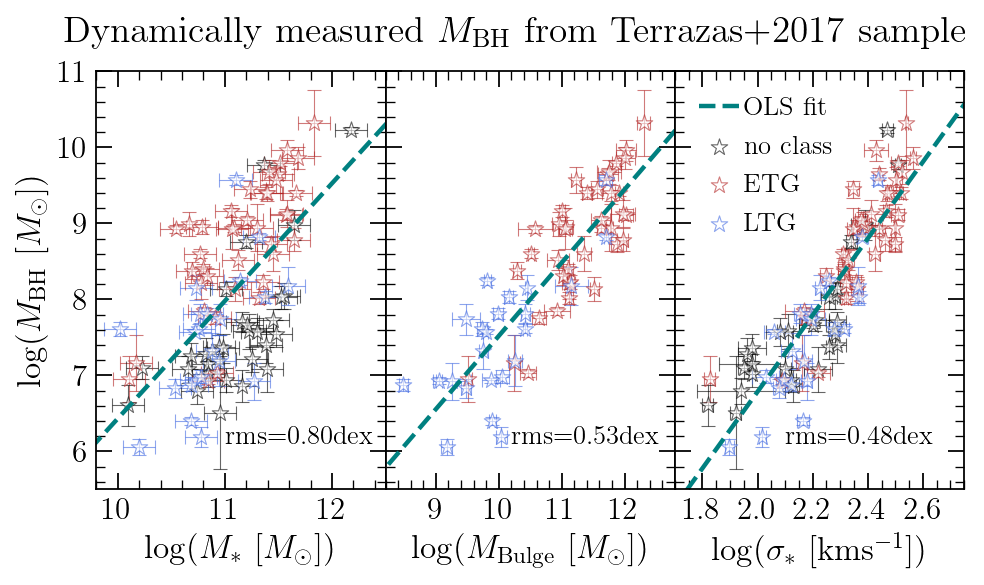
Figure 1: Comparison of scatter in the ${M_{\ast}}$–${M_{\rm BH}}$, ${M_{\rm BH}}$–$M_{\rm bulge}$ and ${M_{\rm BH}}$–$\sigma_{\ast}$ relation in a sample of dynamically measured black hole masses taken from Terrazas et al. (2017). It is clear that the relationship between ${M_{\rm BH}}$ and $\sigma_{\ast}$ is the strongest of the three, supporting the choice of $\sigma_{\ast}$ to estimate black hole masses in our SDSS sample. Please note that the sample of galaxies without ETG/LTG (early-type/late-type galaxy) classification do not have an associated bulge mass measurement.

3.1 $M_{\rm BH}$ estimation in the SDSS

A direct measurement of a supermassive black hole mass requires high resolution spectroscopic observations in order to accurately model the orbital dynamics of gas and stars within its gravitational sphere of influence. Given the complexity of such measurements and objects selection criteria, the current literature can only provide around a hundred dynamically measured ${M_{\rm BH}}$ in massive central galaxies observed in the local Universe (e.g. Terrazas et al., 2016, 2017). Despite their small sample sizes, these studies deliver important inferences about quenching processes, e.g. indicating a connection between quiescence and high black hole mass. When comparing observations with theoretical models, however, large samples are often superior since they allow one to explore the behaviour of statistically average galaxy populations.

Fortunately for this work, the direct measurement studies uncovered an intimate connection between central black holes and their host galaxies (see Kormendy & Ho, 2013, for a review), finding strong correlations between ${M_{\rm BH}}$ and ${M_{\ast}}$(Reines & Volonteri, 2015), $M_{\rm bulge}$ (Häring & Rix, 2004) or $\sigma_{\ast}$ (Hopkins et al., 2007; McConnell & Ma, 2013; Saglia et al., 2016). In Fig. 1 we show a comparison among these three scaling relations for central galaxies in the Terrazas et al. (2017) sample, which indicates that the connection between ${M_{\rm BH}}$ and ${M_{\ast}}$ is the weakest of them all. An ordinary least squares (OLS) fit to logarithmic values shows a RMS scatter of 0.80 dex for the ${M_{\rm BH}}$–${M_{\ast}}$ relation, while in the ${M_{\rm BH}}$–$M_{\rm bulge}$ and ${M_{\rm BH}}$–$\sigma_{\ast}$ relations the scatter is significantly smaller, reaching 0.53 dex and and 0.48 dex respectively.

In lieu of dynamical measurements of black hole masses in our sample, we test a variety of calibrations published in the literature to estimate ${M_{\rm BH}}$ in the SDSS galaxies. We focus primarily on $\sigma_{\ast}$, due to its tightest correlation with the black hole mass, illustrated in Fig. 1. However, we also use a prescription for estimating ${M_{\rm BH}}$ from $M_{\rm bulge}$ in Eq. 9, which allows us to explore a larger number of objects since this parameter does not require a cut on galaxy inclination or a requirement on high S/N of the galactic spectra . We also include separate calibrations for different galaxy morphologies: early-type (ETG) / late-type (LTG) galaxies in Eq. 10 and pseudo-/classical bulges in Eq. 11. These distinct morphologies are associated with different modes of black hole growth (e.g. Kormendy et al., 2011; Kormendy & Ho, 2013) and have been found to exhibit different scaling relations between galactic properties and ${M_{\rm BH}}$ (e.g. Mathur et al., 2012; McConnell & Ma, 2013; Saglia et al., 2016).

In our study we label galaxies with $(B/T)>0.5$ as ETG and $(B/T)\leq 0.5$ as LTG. This criterion was not used directly by McConnell & Ma (2013), who classified galaxy morphology through visual inspection, however Simard et al. (2011) show that a selection in bulge-to-total light ratio of above 0.7 is a good proxy for visual classification of ETGs. This bulge-to-total light ratio corresponds to $(B/T)>0.5$ in mass, as demonstrated by Bluck et al. (2019). Additionally, we also classify bulges as classical when the galaxy’s Sérsic index is greater than 2 and as a pseudobulge otherwise. All parametrisations we use in our study are listed in Eq. 7 through 11 below, along with the intrinsic scatter associated with each relation, denoted as $\epsilon$:

$$\begin{split}\log{M_{\rm BH}}=5.246\times\log{\sigma_{\rm c}}-&3.77\\ &\text{\cite[citep]{(\@@bibref{AuthorsPhrase1Year}{Saglia16}{\@@citephrase{, }}{})}},\ \epsilon=0.417\end{split}$$ (7)

$$\begin{split}\log{M_{\rm BH}}=0.54\times\log{(M_{\rm bulge}/10^{11})}+2.18\times\log{(\sigma_{\rm c}/200)}&+8.24\\ \text{ \cite[citep]{(\@@bibref{AuthorsPhrase1Year}{Hopkins07}{\@@citephrase{, }}{})}},\ \epsilon=0.22&\end{split}$$ (8)

$$\begin{split}\log{M_{\rm BH}}=1.12\times\log{(M_{\rm bulge}/10^{11})}+8.20\qquad\quad&\\ \text{ \cite[citep]{(\@@bibref{AuthorsPhrase1Year}{HaringRix04}{\@@citephrase{, }}{})}},\ &\epsilon=0.30\end{split}$$ (9)

$$\begin{split}\log{M_{\rm BH}}=\begin{cases}5.20\times\log{(\sigma_{\rm c}/200)}+8.39\quad\text{ETG}\quad\epsilon=0.34\\ 5.06\times\log{(\sigma_{\rm c}/200)}+8.07\quad\text{LTG}\quad\epsilon=0.46\end{cases}\\ \text{\cite[citep]{(\@@bibref{AuthorsPhrase1Year}{MM13}{\@@citephrase{, }}{})}}\end{split}$$ (10)

$$\begin{split}\log{M_{\rm BH}}=\begin{cases}4.546\times\log{(\sigma_{\rm c}/200)}-2.030\\ \qquad\qquad\qquad\qquad\text{classical bulge},\ \epsilon=0.348\\ 2.129\times\log{(\sigma_{\rm c}/200)}+2.526\\ \qquad\qquad\qquad\qquad\text{pseudo bulge},\ \epsilon=0.455\end{cases}\\ \text{\cite[citep]{(\@@bibref{AuthorsPhrase1Year}{Saglia16}{\@@citephrase{, }}{})}}\end{split}$$ (11)

where $M_{\rm bulge}$ is given in units of ${\rm M_{\odot}}$ and $\sigma_{c}$ denotes the central velocity dispersion in units of ${\rm kms^{-1}}$. The central velocity dispersion (Jorgensen et al., 1995) is calculated from $\sigma_{\ast}$ via:

$$\sigma_{c}=\sigma_{\ast}\quantity(\frac{R_{\rm bu}/8}{R_{\rm fib}})^{-0.04},$$ (12)

where $R_{\rm bu}$ and $R_{\rm fib}$ denote the bulge and the SDSS fibre radii respectively.

In this work we make use of all calibrations in the SDSS, explicitly showing how our results in Sec. 4 are robust against the exact parametrisation of the observed galaxy scaling relations.

3.2 Gas mass estimation in the SDSS

We follow the molecular gas mas estimation method outlined in Piotrowska et al. (2020), using dust reddening of the optical spectra to infer the mass of molecular hydrogen ($M_{\rm H2}$) in a given SDSS fibre. More specifically, we use an empirical relation between hydrogen number density and colour excess ($E(B-V)$) observed for different lines of sight within the Milky Way (Gudennavar et al., 2012), to estimate the amount of gas associated with the optical extinction observed for each galaxy in our sample. Under the assumption of a uniform foreground dust screen and a linear metallicity dependence in the gas-to-dust ratio the average gas surface density within the fibre, $\Sigma_{\rm gas}$, is given by:

$$\Sigma_{\rm gas}=\quantity[(31.6\pm 1.0)A_{V}+1.0]\quantity(\ifrac{Z_{\odot}}{Z})\ {\rm M_{\odot}{pc^{-2}}}\,,$$ (13)

where $Z$ is the gas phase metallicity, $Z_{\odot}$ is its solar value and $A_{V}=E(B-V)/R_{V}$ is the dust attenuation in the optical $V$-band with $R_{V}\sim 3.1$ for the Milky Way. In this work we use the O3N2 calibration extended to non purely star-forming regions by Kumari et al. (2019) to calculate gas phase metallicity for all galaxies which meet our emission line quality selection criteria.

In order to estimate $A_{V}$ we assume a Galactic extinction curve parametrised by Cardelli et al. (1989) and compare the observed ratio of ${\rm H\alpha}$ and ${\rm H\beta}$ emission line fluxes ($\ifrac{F_{\rm H\alpha}}{F_{\rm H\beta}}$) to its theoretical intrinsic value of 2.86 as determined by Case B calculations in Hummer & Storey (1987). More specifically, we calculate $A_{V}$ using the following formula:

$$A_{\lambda}=\frac{K_{\lambda}}{K_{\rm H\beta}-K_{\rm H\alpha}}2.5\log_{10}\Bigg{(}\frac{{F_{\rm H\alpha}}/{F_{\rm H\beta}}}{2.86}\Bigg{)}\,,$$ (14)

where the $K_{\lambda}=A_{\lambda}/A_{V}$ coefficients are taken from the Cardelli et al. (1989) extinction law ($K_{\rm H\alpha}=0.817,K_{\rm H\beta}=1.164$), however any extinction or attenuation law of choice can be applied in this method.

As we explicitly show in Piotrowska et al. (2020) this method accurately traces hydrogen in its molecular phase and when we compare the molecular gas masses obtained with this method against $M_{\rm H2}$ inferred from the CO emission in the COLDGASS sample (Saintonge et al., 2017), we find an RMS of 0.4 dex and a Spearman correlation strength of 0.84. For a further discussion of the details and robustness of this method we refer the interested reader to Piotrowska et al. (2020).

The use of proxies to estimate black hole and molecular gas masses in the SDSS allows us to extend the sample size by a factor of a thousand in comparison with the more direct measurement studies. This substantial increase in sample size is critical for a statistically robust comparison between the theoretical predictions from the simulations and the observed Universe.

3.3 Random Forest analysis

Given that quenching is a complex process, one expects the connection between large-scale galactic properties and the star-forming state of galaxies to be non-trivial. Hence, an appropriate analysis should not be restricted to a search for power-law relationships and determination of scatter, but rather embrace the non-linear character of the problem along with the whole range of potential parameters involved. A natural approach meeting these criteria is machine learning, which allows us to explore and identify relationships among our data without making a priori assumptions about said relationships.

In particular, we opt for a Random Forest (RF) classifier to ask which of the following variables: ${M_{\rm BH}}$, ${M_{\rm halo}}$  ${M_{\ast}}$ or ${\dot{M}_{\rm BH}}$ (in simulations only) has the most influence on determining whether a galaxy is star forming or quiescent. We choose these particular quantities because each of them is associated with a separate quenching mechanism under consideration. ${M_{\ast}}$ serves as a proxy for the strength of supernova feedback, ${M_{\rm halo}}$ is directly linked to CGM gas heating via virial shocks, ${M_{\rm BH}}$ traces the integrated energy input into the gas via AGN feedback and ${\dot{M}_{\rm BH}}$ describes the instantaneous influence of AGN on its surroundings, measuring the feedback energy output at a given snapshot.

Random Forest classification overview

A Random Forest classifier is a simple machine learning algorithm which assigns discrete labels (‘classes’) to elements within a dataset, using a set of inputs (‘features’) for each element. It is a form of supervised learning, which means that each element in the dataset used for algorithm training (i.e. the algorithm learning process) has a class label assigned to it. To put this in the context of our dataset, each element is a single galaxy labelled as ‘star-forming’ or ‘quenched’, based on its specific star formation rate with the default classification threshold chosen as $\log({\rm sSFR/yr^{-1}})=-11$ . The input features for each object are ${M_{\rm halo}}$, ${M_{\ast}}$ and ${M_{\rm BH}}$ and the RF learns how to best assign the ‘quenched’ and ‘star-forming’ labels to galaxies given all these three masses.

One of the main advantages of a Random Forest is its straightforward architecture. This property of the RF allows one to follow the learning logic throughout the algorithm and removes the risk of a ‘black box’ approach commonly associated with more elaborate machine learning techniques. Most importantly for our research, however, this straightforward architecture enables an explicit calculation of the relative importance of each input feature for determining the final classification, referred to as the feature importance. Putting this in a relevant context, once the RF learns to classify galaxies into star-forming and quenched, we can then calculate how important ${M_{\rm halo}}$, ${M_{\ast}}$ and ${M_{\rm BH}}$ were for separating objects into these two categories. We can also directly check how the classification was performed and even visualise the exact structure of the decision-making within the algorithm.

A machine learning Forest, by analogy with a physical one, is a collection of multiple decision trees. A single tree consists of a series of splits on a dataset, each of which results in two subsets. These subsets in RF nomenclature are known as ‘nodes’ and hence the tree begins with a ‘root’ node (the whole input dataset) and grows through subsequent splits on ‘parent’ nodes into ‘daughter’ nodes. These splits are performed by choosing a boundary value in one of the input features and each boundary value & feature combination is optimised to yield daughter nodes more homogeneous than the parent one, i.e. aiming to deliver subsets consisting of only a single class.

There are several different ways in which trees determine the optimal splits. In our RF architecture we choose to minimise Gini index $G(n)$, which measures how often drawing an object from a daughter node at random would result in a misclassification. The Gini index is defined as:

$$G(n)=1-\sum^{J}_{i=1}p_{i}(n)^{2}\,,$$ (15)

where $p_{i}(n)$ is the probability of selecting an element with class $i$ when taking a random draw from elements occupying a node $n$. The total number of available classes is given by $J$ and in our RF $J=2$. The Gini index evaluates to 0 for entirely pure daughter nodes and takes a maximum value of $0.5$ in the case of a random draw of each of the two classes in a daughter node being equally probable. The trees then grow in depth by choosing feature & boundary value combinations which minimise $G(n)$ (maximise the reduction of impurity) at every split. This exponential growth continues until a tree reaches a user-defined maximum depth or until all elements in the dataset occupy their own individual ‘leaves’ (terminal nodes not subject to further splitting). Once the tree is complete, each element is assigned a classification probability based on the distribution of classes within a given leaf.

The true predictive power of a Forest comes from its Randomness. A collection of weakly correlated outcomes of individual trees creates an ensemble prediction which outperforms that of any given tree. Differences among the trees render the combined result less sensitive to outliers and peculiarities of the parent dataset, allowing the algorithm to find general patterns present within the data. This property underlies the main application of RFs - predicting classification of previously unseen objects given the complex, general relationships between features and classes learned from a training dataset.

What makes the Forest Random is a random sampling of the data which comprise root nodes of individual decision trees. The number of trees in a forest as well as the sampling method are determined by a user and we choose to draw a 100 bootstrap samples with replacement to construct 100 trees. Additionally, one can further increase the level of randomness within individual trees themselves by forcing the algorithm to only consider a random subset of features to split on at each node. Empirical tests suggest that restricting the number of features to as few as two at each node makes the algorithm more robust with respect to noise in classification problems (e.g. Breiman, 2001). Hence, it is a common practice to randomly choose $\sqrt{p}=2$ features to split on at every node in RF classifiers, where $p$ is the number of input features (e.g. Hastie et al., 2009). In contrast, allowing the algorithm to choose from all features at every split is most effective for isolating causality between the input features and classification labels, as shown explicitly by Bluck et al. (2021). We perform our analysis both using all input features at every node and selecting a random sample of $\sqrt{p}$ features to find that our results are consistent between the two forest designs. However, in the interest of brevity we only present results using all input features in Sec. 4.2 and show the other forest architecture outcome in Appendix B.

Training and validation samples

Table 1: Summary of the forest parameters and sample properties in our RF analysis. The $\langle{\rm AUC}\rangle$ is the median AUC (Area Under the Curve - a measurement of algorithm performance; equal to 1.0 for a perfect classifier and to 0.5 for a random guess) of the test set, while $\gamma$ denotes the min_samples_leaf hyperparameter optimised to achieve the highest AUC score in a given sample.

Data set	Input sample size	# passive objects	$\langle{\rm AUC}\rangle$	$\gamma$
SDSS	148 954	153 550	0.85	145
SDSS HR04	321 522	174 425	0.86	117
SDSS gas	13 104	6552	0.98	40
EAGLE	1786	893	0.81	148
Illustris	1224	612	0.98	5
TNG	2778	1389	0.98	15

The main task required of an RF algorithm is finding an optimal general relationship between the class label and input features for each element in a dataset, which can then be used to make predictions about previously unseen data. Hence, the RF is first trained using a training set drawn from the data and its performance is then evaluated by quantifying the accuracy of predicted classifications on a test set.

In our study, both the training and test sets are drawn from samples of galaxies selected according to the criteria listed in Sec. 2.3 for each simulated and observed local universe. In order to ensure that the algorithm is not driven by either the star-forming (SF) or passive (PA) population which may dominate a given data set, we always consider an equal number of SF and PA galaxies in input samples for the RF. We hence create a ‘balanced sample’ consisting of 50% PA and 50% SF galaxies by randomly choosing a subset of the larger population, such that the numbers of passive and star-forming galaxies are equal. Such a sample results in a better performance of the classifier by maximising the number of splits with a meaningful decrease in impurity. This approach also leads to a more intuitive interpretation of the results, especially when we focus on the relative importance of input features for a given classification, rather than the predictive power of the algorithm.

The SDSS sample is dominated by quiescent galaxies and hence in order to construct a balanced input for the RF we include all SF galaxies and subsample the PA population. In simulations the situation is reversed because their galaxy populations are dominated by star-forming objects. Table 1 summarises the process of sample balancing by comparing the final input RF sample size against the number of passive galaxies in a given data set. In the simulations the input sample size is twice the number of passive objects in the whole sample, showing that the algorithm is trained on the whole quiescent population and on a random subset of the star-forming one. In contrast, the SDSS galaxies are mostly passive and hence the star-forming population is used in full, while the quiescent objects are randomly subsampled. The ‘SDSS HR04’ data set refers to RF runs with ${M_{\rm BH}}$ estimated from $M_{\rm bulge}$ according to Eq. 9 and does not require an inclination cut on disk-dominated galaxies, which preferentially removes star-forming objects from the RF samples using $\sigma_{\ast}$-derived ${M_{\rm BH}}$. The ‘SDSS gas’ data set describes the input for the star-forming/passive classification using $f_{\rm gas}$ and SFE as input features. In this case the bulk of passive SDSS galaxies is removed via S/N cuts on emission line fluxes and hence the input sample size is dictated by the leftover quiescent objects.

Once the sample consists of an equal number of star-forming and passive galaxies, we proceed to randomly split it into a training and a test set with an equal number of objects in each. This way we maximise the RF training opportunity and ensure its exposure to a large test set of previously unseen data. Finally, in order to account for the randomness in our balanced sample selection, we repeat the RF experiment 500 times for each data set, subsampling the larger of populations at random with each repetition. Each of the experiments results in different feature importances which together yield a set of importance distributions (one for each feature among ${M_{\rm BH}}$, ${M_{\rm halo}}$ and ${M_{\ast}}$). We then take our final result for a given feature to be the median value of its importance distribution and show errorbars spanning the 5th and 95th percentiles of said distribution.

Feature importances and algorithm optimisation

The main purpose of our RF analysis is the identification of the most important quenching parameter, i.e. estimating the feature importances. This can be done in various ways (see Chapter 6 in Louppe, 2014, for a summary) and in our case is done by calculating the Mean Decrease in Impurity, otherwise known as the Gini Importance. This metric calculates each feature importance as the sum over the number of splits within the algorithm which include the feature, weighted by the number of elements the feature splits. More precisely, the relative importance $I_{R}(k)$ of feature $k$ is calculated via:

$$I_{R}(k)=\frac{I_{k}}{\sum_{j}I_{j}}=\frac{\sum_{n_{k}}N(n_{k})\Delta G(n_{k})}{\sum_{n}N(n)\Delta G(n)}\,,$$ (16)

where

$$\Delta G(\rm{parent})=G({\rm parent})-G({\rm daughter})$$ (17)

is a change in the Gini index between a daughter and a parent node. The $n_{k}$ sum is performed over all splits the feature $k$ contributes to while the $n$ sum corresponds to all splits within the forest. The change in Gini index is also weighted by the number of elements in a given parent node $N$, which results in a higher importance calculated for features which have an impact on a larger number of elements in the dataset.

Another popular method for estimating feature importance relies on randomising the input feature values and evaluating the impact this action has on the final classification outcomes. This method, called the permutation importance, breaks the connection between features and classification labels established through training and hence a drop in the algorithm classification accuracy indicates how much a given label depends on a given feature (Breiman, 2001). We check that our main conclusions are consistent with the two importance calculation techniques and present results based on Gini importance in Sec. 4.2. For a detailed discussion on the Gini importance and its broader applications we refer the interested reader to Bluck et al. (2021).

A final point to consider in the Random Forest architecture is the risk of over-fitting, which occurs when the algorithm perfectly learns the relationship between features and class labels in a given training set and then spectacularly fails upon exposure to previously unseen data. In such a scenario the performance of an RF would be ranked very high for the training set and then very low for a test set in our experiment. One can avoid over-fitting by controlling the number of elements (galaxies) which comprise the leaves of individual trees. By allowing the trees to grow without constraints, each leaf node ends up occupied by a single galaxy only and hence the algorithm perfectly learns all the patterns within a training data set and achieves a high score in a training set. In contrast, when one imposes a minimum occupancy for a leaf node, the algorithm can only learn the general patterns within the dataset recovered both in the training and testing sets, which come at a price of a lower classification accuracy within the training set. Hence, controlling the minimum number of elements which comprise a leaf node in a tree allows one to avoid over-fitting in the Random Forest algorithm.

In order to optimize the performance of our RF classifier we use the Receiver Operating Characteristics (ROC) graphs (Fawcett, 2006), which show the True Positives Rate (TPR) as a function of False Positives Rate (FPR). The output of our RF is a set of class probabilities (i.e. how likely a given galaxy is to be classified as quenched), hence the ROC curve is computed by varying probability thresholds for passive classification and calculating their corresponding TPR & FPR. We further reduce the curves to a single parameter by taking the area under the curve (AUC) in the ROC space. The AUC parameter ranges between ${\rm AUC}=0.5$ for a classifier equivalent to a random class assignment and $\rm{AUC}=1.0$ for a perfect classification algorithm. In this work we optimise the Random Forest architecture to maximise $\rm AUC_{train}$ under the criterion that $\rm AUC_{train}-AUC_{test}\leq 0.01$ in order to avoid the risk of over-fitting in the algorithm. In this way we maximise the performance of our Random Forest on both the training and test data sets, making sure the algorithm is generalisable and performs well on previously unseen data (see Bluck et al., 2020a, b, for examples of this approach).

We implement the RF algorithm using the RandomForestClassifier class in the sklearn.ensemble module of the scikit-learn (Pedregosa et al., 2011) open source machine learning package for python. As mentioned before, we set the max_features value to either "sqrt" or "None", n_estimators $=200$ and optimise the min_samples_leaf parameter to maximise AUC in all data sets individually, while retaining default values for all other parameters. The final min_samples_leaf values along with AUC scores are presented in Table 1.

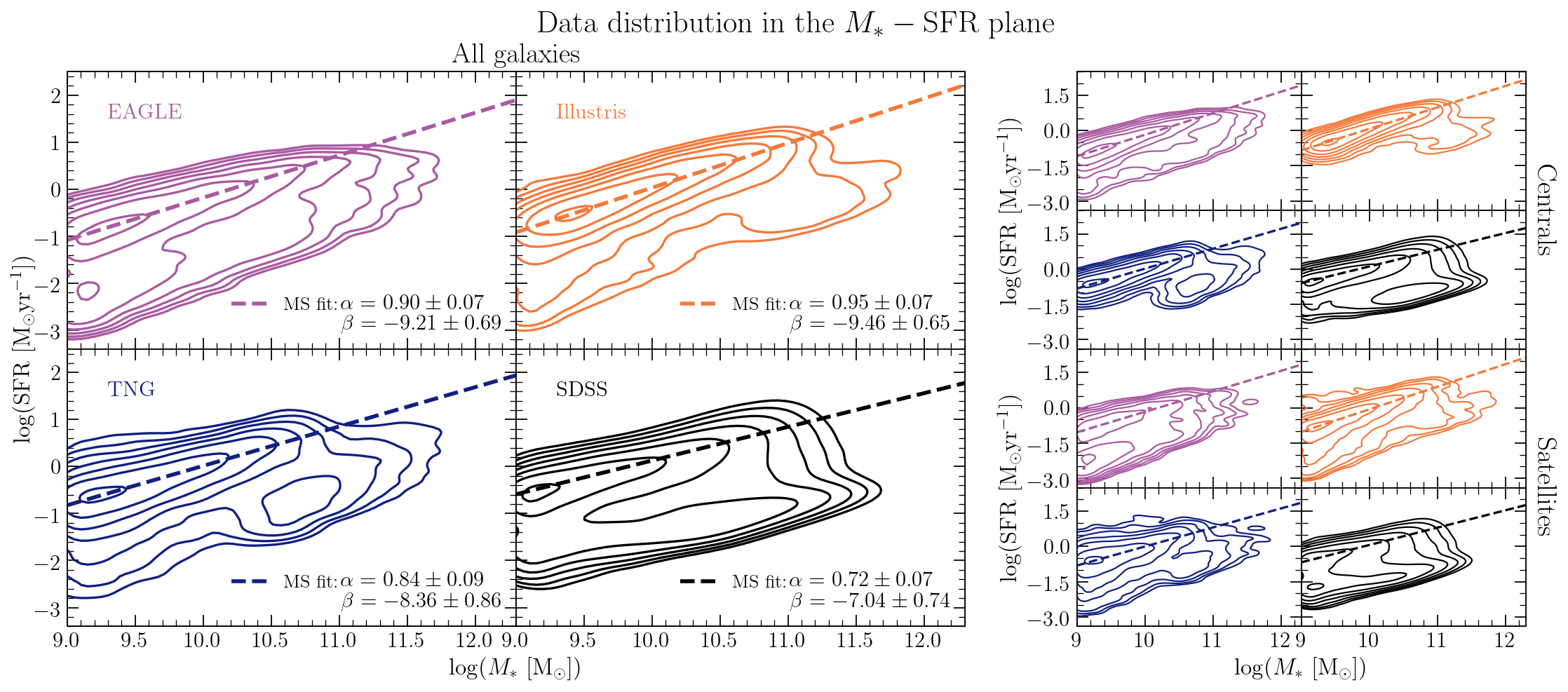
Figure 2: The distribution of galaxies in the $M_{\ast}-{\rm SFR}$ plane for EAGLE (purple), Illustris (orange), TNG (blue) and SDSS (black). Dashed lines show ordinary least squares fits to the star-forming Main Sequence defined as galaxies with log(sSFR/${\rm yr^{-1}}$) $>-10.5$. Left panel: all galaxies in the sample, panels on the right: galaxies split into centrals (top) and satellites (bottom). MS fits in the whole population agree within uncertainties in the simulations and their slopes are consistently steeper than in the SDSS. It is also apparent that for both Illustris and TNG passive centrals are primarily high-mass objects, while EAGLE seems to have quenched centrals spanning all mass ranges. Please note: low sSFR values in the simulations are redistributed by drawing from the SDSS passive sequence distribution to aid visual comparison (see Fig. 17 in appendix A). The SDSS contours were corrected to account for the Malmquist bias.

4 Results

We begin our analysis with a qualitative comparison of observed and simulated local galaxies by considering the data distributions in the $M_{\ast}-{\rm SFR}$ plane, presented as density contours in Fig. 2. In order to fairly compare the observed and simulated universes, we weight the distribution of SDSS objects in the plane by the inverse of the maximum comoving volume they can be observed within, given their intrinsic brightness and the magnitude limit of the survey. This way we account for the preferential loss of low-luminosity objects with increasing redshift of observation, known as the Malmquist bias (Malmquist, 1922). In simulations, we make sure to show all galaxies in a finite range of the logarithmic SFR axis by relocating objects with extremely low specific star formation rates (sSFR). To this end, for every galaxy with log(sSFR/${\rm yr^{-1}}$) $<-12$ we draw an sSFR value from the observed distribution in the SDSS passive sequence (see appendix A for details). This manoeuvre is only intended for presentation purposes, in order for us to make a fair visual comparison of galaxy populations between simulations and the SDSS. These redistributed values can then be treated as upper limits on SFR, much like the SFR estimates in the SDSS passive sequence derived from the strength of the D4000 break, instead of ${\rm H}\alpha$ fluxes. In this way we avoid neglecting low-SFR objects in simulations or, alternatively, extending the $\log(\rm{SFR})$ range to arbitrarily large negative values.

In Fig. 2 we present density contours of galaxy distributions in the $M_{\ast}-{\rm SFR}$ plane, which show very good qualitative agreement across all data sets for all galaxies (left panel), centrals (top right panel) and satellites (bottom right panel). All simulation suites have well-pronounced star-forming Main Sequences (MS) and less abundant passive populations, much like the SDSS. However, the jagged contours indicate a smaller coverage of the parameter space in the simulations compared to the observations. Illustris and TNG also show a hint of transition between the dominance of star formation at low ${M_{\ast}}$ and quiescence at high ${M_{\ast}}$. This feature is even more pronounced in the subset of central galaxies, where quenched low-${M_{\ast}}$ objects are absent in these suites. The raw SDSS measurements exhibit a similar behaviour in centrals, however once the volume correction is accounted for, the population of quiescent central galaxies spans the whole range in stellar mass, peaking at around $\log(M_{\ast}/{\rm M_{\odot}})=10.5$. Satellite galaxies can be both quenched and star-forming at all ${M_{\ast}}$ in all data sets. The distribution of satellites in EAGLE follows that of the SDSS, peaking at low stellar mass objects. In Illustris and TNG no such behaviour is observed and their distribution is dominated by star-forming objects at all ${M_{\ast}}$.

Table 2: Summary of OLS fit parameters to the star-forming MS.

		SDSS	EAGLE	Illustris	TNG
all	$\alpha$	$0.72\pm 0.07$	$0.90\pm 0.07$	$0.95\pm 0.07$	$0.84\pm 0.09$
	$\beta$	$-7.04\pm 0.74$	$-9.21\pm 0.69$	$-9.46\pm 0.65$	$-8.36\pm 0.86$
all with scatter		$\alpha$	$0.89\pm 0.09$	$0.92\pm 0.09$	$0.82\pm 0.10$
		$\beta$	$-9.03\pm 0.93$	$-9.16\pm 0.94$	$-8.18\pm 1.05$
cen	$\alpha$	$0.71\pm 0.07$	$0.92\pm 0.07$	$0.91\pm 0.06$	$0.85\pm 0.08$
	$\beta$	$-6.98\pm 0.71$	$-9.33\pm 0.67$	$-9.06\pm 0.57$	$-8.46\pm 0.75$
sat	$\alpha$	$0.74\pm 0.08$	$0.87\pm 0.11$	$0.96\pm 0.08$	$0.81\pm 0.13$
	$\beta$	$-7.31\pm 0.81$	$-8.89\pm 1.10$	$-9.66\pm 0.81$	$-8.10\pm 1.24$

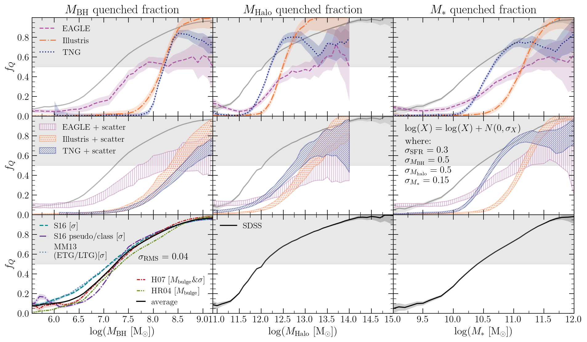
Figure 3: Comparison of quenched fractions ($f_{Q}$) as function of $M_{\rm BH}$, $M_{\rm halo}$ and $M_{\ast}$ in simulations (top row), in simulations with observation-like scatter added (middle row) and observations (bottom row). In the SDSS $M_{\rm BH}$ quenched fraction calculation five different $M_{\rm BH}$ calibrations are included, listed in the legend. The simulation panels also include SDSS curves (solid gray lines) to aid direct comparison. For all quantities, the simulations show steeper trends than SDSS, with the exception of EAGLE, which shows shallower slopes and levels off at $f_{Q}\sim 0.6$. Adding scatter to each of the quantities listed in the figure flattens the simulated curves, making the transition significantly less abrupt for Illustris and TNG. Nevertheless, the simulations still under-predict quenching for all parameters (as quantified in Table 3). The different $M_{\rm BH}$ calibration curves demonstrate that the conclusions drawn from SDSS do not strongly depend on the choice of $M_{\rm BH}$ indirect inference method.

Table 2 summarises MS fit parameters corresponding to dashed lines in Fig. 2. We perform an OLS fit to $\log({\rm SFR})=\alpha\log(M_{\ast})+\beta$ for Main Sequence objects selected with a log(sSFR/${\rm yr^{-1}}$) $>-10.5$ criterion. We divide MS galaxies into 0.1 dex bins in $\log(M_{\ast})$ for ${9<\log(M_{\ast}/{\rm M_{\odot}})<11}$ and fit to the median $\log({\rm SFR})$ values in each bin. In order to estimate uncertainties on $\alpha$ and $\beta$ we use the median absolute deviation (MAD) of $\log({\rm SFR})$ in the bins, treating them as heteroskedastic, independent errors on median $\log({\rm SFR})$.

Table 2 shows that MS fits across all simulations agree with each other within the calculated uncertainties, while the SDSS shows a significantly shallower slope. When we focus on the central-satellite split we notice that in EAGLE and TNG the satellite MS is flatter, while for Illustris and SDSS it is steeper, however slopes in the two populations agree within their uncertainties for all data sets. Finally, we check how the Main Sequence fits to the whole population change in the simulations when we add observation-like scatter to the raw data. For each simulated galaxy we add a random draw from a Gaussian to both $\log({\rm SFR})$ and $\log(M_{\ast})$ to imitate the addition of measurement uncertainty present in the observations. The widths of scatter distributions are $\sigma_{M_{\ast}}=0.15$ and $\sigma_{\rm SFR}=0.3$ respectively to reflect the median uncertainties in the SDSS. The resulting MS slopes are flatter in all three simulations, however not flat enough to match the SDSS. They also agree with the raw MS fits within their estimated errors.

Our simplistic method to fitting the MS allows us to compare SDSS and simulations without additional selection choices on emission line ratios and S/N values, which are not available in the simulation suites. This approach is similar to the objective MS definition in Renzini & Peng (2015) and for the SDSS yields parameters consistent with their study. The broad qualitative agreement between simulations and observations in the $M_{\ast}-{\rm SFR}$ distributions of centrals and satellites is promising. We also note that the quantitative discrepancies between the observed and simulated Main Sequences can be significantly reduced when different techniques are applied to estimating SFR in the observations (e.g. as demonstrated by Nelson et al., 2021, for TNG50 at redshift $z=1$). Hence, encouraged by this initial comparison we investigate similarities and differences between the simulated and observed data sets in more detail in the subsequent sections.

4.1 Behaviour of quenched fractions and sSFR as a function of ${M_{\rm BH}}$, ${M_{\rm halo}}$ and ${M_{\ast}}$

Table 3: Parameter values at which quenched fractions reach $f_{Q}=0.5$. All values have an uncertainty of $\pm 0.2\,{\rm dex}$. Values in brackets show how adding observation-like scatter to simulations influences the point at which the galaxy population is mostly quiescent.

	SDSS	EAGLE	Illustris	TNG
$\log(M_{\rm BH})$	7.2	7.8 (8.1)	8.2 (8.4)	8.2 (8.6)
$\log(M_{\rm Halo})$	12.0	13.2 (13.6)	12.5 (13.0)	12.2 (12.8)
$\log(M_{\ast})$	10.4	11.2 (11.1)	11.1 (11.1)	10.6 (10.6)

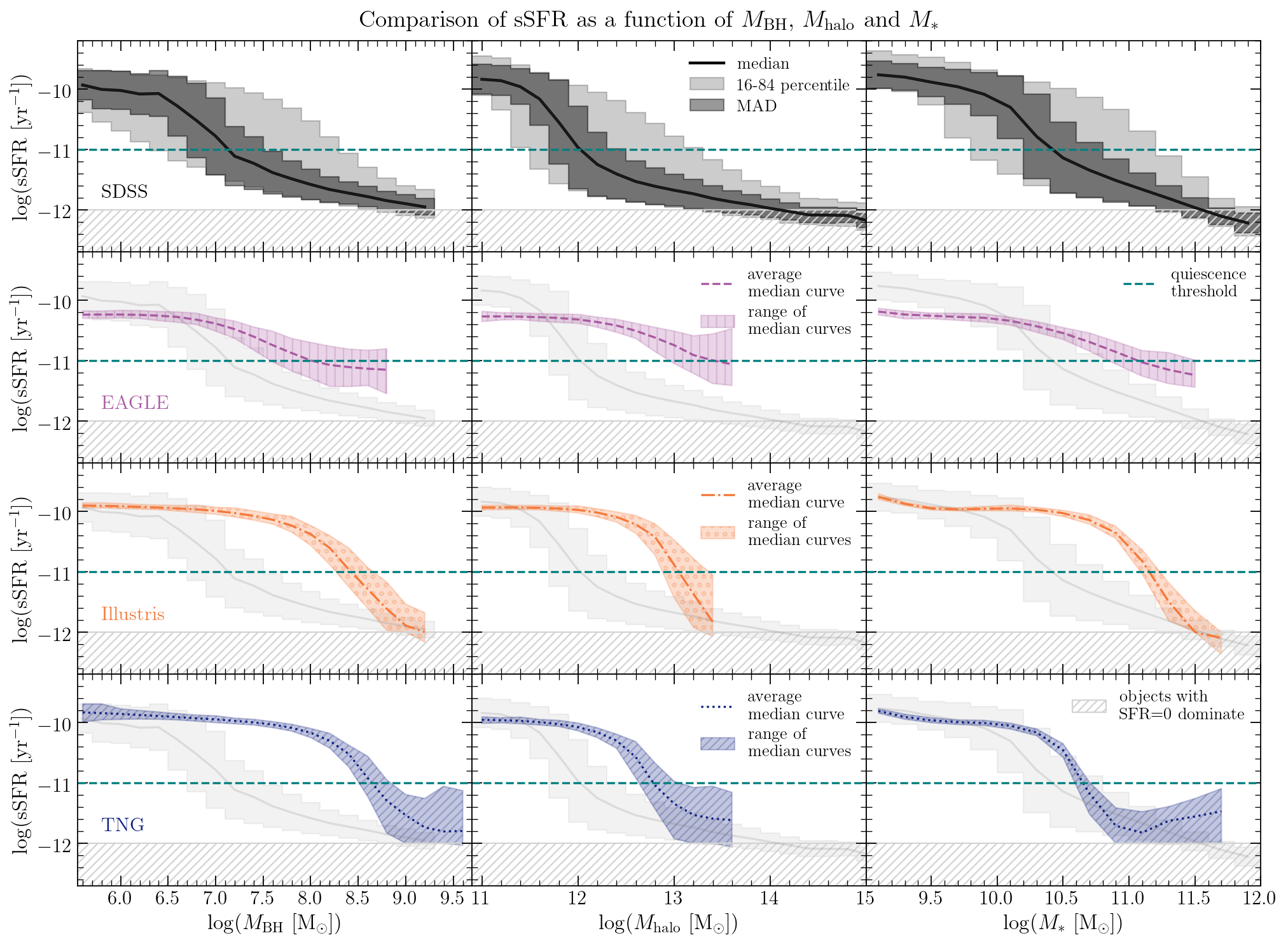
Figure 4: Comparison of sSFR as a function of ${M_{\rm BH}}$ (left column), ${M_{\rm halo}}$ (middle column) and ${M_{\ast}}$(right column) in the SDSS and in the simulations. In the SDSS the calculation includes $1/V_{\rm max}$ and inclination corrections and the shaded regions correspond to the median absolute deviation (MAD) and the 16-84 percentile range of sSFR distribution in a given bin. The hatched coloured regions in the simulations show the range of median curves resulting from 500 realisations of adding random scatter to the data to mimic measurement uncertainty. The minimum number of galaxies in a given 0.2 dex bin is 20. In EAGLE all curves show similar slopes to the SDSS, however they hardly reach log(sSFR/${\rm yr^{-1}}$) $=-11$, highlighting the lack of quenched objects in the suite. Illustris and TNG show steeper slopes than the observations, quenching galaxies at higher values of all parameters than the SDSS.

We first look at the transition to quiescence by comparing quenched fractions $f_{Q}(X)$ calculated as a function of $X=M_{\rm BH}$, ${M_{\rm halo}}$ and ${M_{\ast}}$. We define the quenched fraction as :

$$f_{Q}=\frac{n_{{\rm Q},i}}{n_{{\rm Q},i}+n_{{\rm SF},i}}$$ (18)

where $i$ labels a bin in quantity $X$, and $n_{{\rm Q},i}$, $n_{{\rm SF},i}$ are the number of quenched and star-forming objects in a given bin respectively. Each bin is 0.4 dex wide, while bin centres are separated by 0.1 dex in order to obtain smoother curves. In simulations $n_{i}$ is simply the number of galaxies in a given population, while in the SDSS we correct for the inclination cut and the Malmquist bias by substituting $n_{i}$ with:

$$n_{i}=\sum_{j}\omega_{j},\qquad\text{where}\ \omega_{j}=\frac{w_{{\rm inc},j}}{V_{{\rm max},\,j}}.$$ (19)

where $V_{\rm max}$ is the maximum comoving volume a galaxy can be observed in, $j$ enumerates objects of a given population in a bin and $w_{\rm inc}$ is a correction factor associated with inclination selection, defined in Eq. 6. We verify that $w_{\rm inc}$ achieves its intended effect by comparing the survey ${M_{\ast}}$ quenched fractions with and without inclination selection criteria and corrections, finding very good agreement between the two resulting curves.

Fig. 3 presents quenched fractions as a function of ${M_{\rm BH}}$, ${M_{\rm halo}}$ and ${M_{\ast}}$ for all simulations together in the top panel and the SDSS in the bottom panel. It is apparent that quenched fractions show an increasing trend with all quantities both in the observed and simulated universes. Illustris and TNG show more rapid transitions between star forming and quenched populations in all parameters, demonstrated by visibly steeper curves than those seen in the SDSS. The steep $f_{Q}(M_{\ast})$ curves in these two suites are consistent with recent studies by Donnari et al. (2021a) and Donnari et al. (2021b), where the authors use a different prescription for identifying quenched centrals in Illustris and TNG100. EAGLE breaks this pattern in simulations by showing flatter curves more akin to observations, however it fails to recover $f_{Q}\sim 1$ at high parameter values, hovering at $f_{Q}\sim 0.6$ instead. Hence, in EAGLE there remains a significant fraction of star forming systems at even the highest values of ${M_{\ast}}$, ${M_{\rm halo}}$ and ${M_{\rm BH}}$. We also notice that simulations, on average, tend to transition into the quiescence-dominated regime later than the SDSS, reaching the grey shaded region at higher parameter values. Table 3 lists ${M_{\rm BH}}$, ${M_{\ast}}$ and ${M_{\rm halo}}$ values at which all curves reach the $f_{Q}=0.5$ mark, clearly demonstrating this behaviour.

Fig. 3 also addresses the uncertainty associated with our choice of black hole mass calibration in the leftmost bottom panel, where we compare quenched fractions resulting from different inference methods. Each curve is calculated for ${M_{\rm BH}}$ estimated from central velocity dispersion, bulge mass or combination of the two, following prescriptions in Eq.7-11. In the case of Häring & Rix (2004) calibration (labelled HR04 in the panel) the galaxy sample is not subject to an inclination cut, as it is not relevant for the measurement of $M_{\rm bulge}$. All resulting $f_{Q}-M_{\rm BH}$ relations agree well with one another with an RMS scatter around the mean quenched fraction of only $\sigma_{\rm RMS}=0.04$. This panel clearly demonstrates that the relationship between $f_{Q}$ an ${M_{\rm BH}}$ is largely invariant to the choice of calibration. This means that regardless of whether we use different scaling for early and late type galaxies, choose a different proxy ($\sigma_{\ast}$ or $M_{\rm bulge}$) or introduce additional sample selection criteria, our conclusions remain unaffected for black hole mass in the SDSS.

Finally, we check how the measurement uncertainty present in observations would demonstrate itself in the $f_{Q}$ relationships calculated for the simulations. To this end we add a random Gaussian noise to the measurements of SFR, ${M_{\ast}}$, ${M_{\rm halo}}$ and ${M_{\rm BH}}$ to mimic the measurement uncertainties in the SDSS. More specifically, for each simulated galaxy, we add a random draw from a Gaussian centred on 0 with a standard deviation $\sigma=\sigma_{X}$ in each parameter of interest $X$. The $\sigma_{X}$ values were chosen to reflect the median random errors in the corresponding SDSS measurements and are listed in the rightmost middle panel in Fig. 3. The random error in SFR is only added for galaxies with log(sSFR/${\rm yr^{-1}}$) $>-11$, since SFRs in the passive population in the SDSS are estimated using D4000 and hence treated as upper limits throughout our analysis. Hatched regions in the middle panel of Fig. 3 show the range of $f_{Q}$ curves resulting from 500 random realisations of simulated galaxies with scatter added as per the description above. These regions demonstrate that the addition of random uncertainty to the simulated data flattens $f_{Q}$ curves towards observation-like shapes. The flattened curves, however, still reach $f_{Q}=0.5$ at higher parameter values than in the SDSS, like it was previously seen in the raw results.

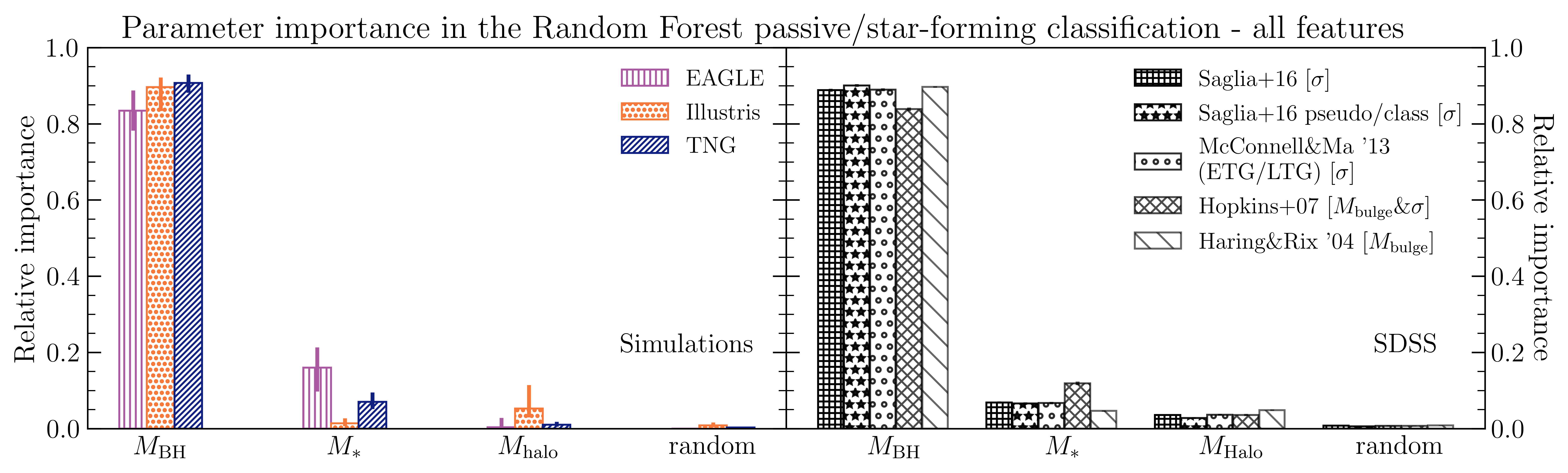
Figure 5: Feature importances for ${M_{\rm BH}}$, ${M_{\rm halo}}$ and ${M_{\ast}}$ extracted from a RF classification of central galaxies into star-forming and quenched categories. Bar heights represent the importance of each parameter for the classification outcome in a trained forest, and they sum up to one in each data set. Error bars indicate the 5th and 95th percentiles of the distribution in parameter importance drawn from 500 realisations of the experiment. Left panels: results in simulations. It is apparent that, irrespective of the model differences, all simulations predict ${M_{\rm BH}}$ to be the most important galactic property discriminating between the star-forming and quenched populations. Right panels: results in the SDSS with ${M_{\rm BH}}$ estimated using calibrations in Eq. 7-11. It is clear that ${M_{\rm BH}}$ dwarfs other parameters in its connection with quiescence, regardless of the choice of calibration.

In Fig. 4 we take a different look at how quenching progresses with increasing ${M_{\rm BH}}$, ${M_{\rm halo}}$ and ${M_{\ast}}$. To this end we show how the sSFR changes as a function of each of those parameters, comparing the SDSS observations with simulation results. In order to fairly compare all data sets, we use EAGLE, Illustris and TNG post-processed to account for random measurement errors in the observations, like we did in the middle panel of Fig. 3. The median curves in the SDSS include $1/V_{\rm max}$ and inclination corrections, which brings all rows in the figure to an equivalent footing. When we look at the observations alone, we see that sSFR decreases with increasing ${M_{\rm halo}}$, ${M_{\rm BH}}$ and ${M_{\ast}}$, as expected from our analysis of quenched fractions. Halo mass shows the steepest evolution in sSFR with the majority of ${M_{\rm halo}}$ range covered by passive galaxies, following the quenching threshold at $\log(M_{\rm halo}/{\rm M_{\odot}})\approx 12$ seen earlier in the $f_{Q}$ plots.

In the second row of Fig. 4 we compare EAGLE (coloured hatched regions) to the SDSS (light gray shaded regions) and notice that all curves in the suite begin 0.2-0.4 dex lower and have shallower slopes than the observations. The striking lack of quenched objects apparent earlier in Fig. 3 is also highlighted here by the median curves reaching a lower limit of log(sSFR/${\rm yr^{-1}}$) $\approx-11$, in contrast with the other two suites. The Illustris and TNG curves have steeper slopes than the observations in all variables among ${M_{\rm BH}}$, ${M_{\rm halo}}$ and ${M_{\ast}}$ and clearly show that quenching occurs at higher parameter values than in the SDSS. These suites, however, match the observed curves at low values of ${M_{\ast}}$, ${M_{\rm halo}}$ and ${M_{\rm BH}}$, with ${M_{\ast}}$ showing good agreement over the broadest range of values. When we compare the simulations among each other, we find that TNG performs slightly better than Illustris and EAGLE, however none of the suites shows a close agreement with the SDSS.

One important conclusion we draw from Fig. 4 is that none of the three state-of-the-art cosmological simulations are able to correctly predict the trends in sSFR with ${M_{\rm BH}}$, ${M_{\rm halo}}$ and ${M_{\ast}}$ observed in the local Universe. This statement is true for a fair comparison between simulations and observations, where simulated data are augmented with observational realism and the observed galaxy populations are corrected for the effects of survey magnitude limits and inclination cuts. The relationship for which predictions match the SDSS most closely is ${M_{\ast}}$ and sSFR, while for ${M_{\rm halo}}$ and ${M_{\rm BH}}$ the onset of quenching is predicted at much higher parameter values than it is observed (in all simulations). This interesting contrast shows how tuning the models to recover observables like the galaxy stellar mass function results in reasonable predictions for related secondary relationships, e.g. the behaviour of sSFR as a function of ${M_{\ast}}$. The lack of similar constraints from black hole mass is also apparent, since the simulations struggle more to recover the observed relations between ${M_{\rm BH}}$ and sSFR. Hence including these observational constraints from Fig. 3 in future model optimisation can potentially prove valuable for the development of the new generation of cosmological simulations.

Figs. 3 & 4 together inform us about a strong positive association between quenching and ${M_{\ast}}$, ${M_{\rm halo}}$ and ${M_{\rm BH}}$ in all simulations and in the observations. When we compare the simulated universes to the observed Universe in the SDSS, we find qualitatively similar trends in both which are matched quantitatively with a varying degree of success. When we focus on ${M_{\ast}}$ trends only, the TNG result seems to be the closest match with the observations, capturing the transition towards quiescence with increasing parameter values most reliably. When we then look at ${M_{\rm BH}}$, it is the EAGLE suite which shows the closest trends to the SDSS. However, EAGLE struggles to definitively quench galaxies at high black hole masses.

Although $f_{Q}$ and sSFR trends provide an interesting insight into the differences between EAGLE, Illustris and TNG, they do not indicate which among ${M_{\rm BH}}$, ${M_{\rm halo}}$ and ${M_{\ast}}$, if any, are responsible for regulating galaxy quenching. We thus move on to using machine learning techniques in the next section, in order to answer this fundamental question.

4.2 Random forest classification

In order to find out which galactic parameter among ${M_{\rm BH}}$, ${M_{\rm halo}}$ and ${M_{\ast}}$ is the most predictive in determining whether a galaxy is star-forming or quenched, we perform a series of Random Forest classifications described in detail in Sec. 3.3. We conduct this machine learning experiment consistently in both simulations and the observations, repeating the training and testing sequence 500 times for each data set. In this way we account for the random subsampling of the more numerous population between the star-forming and quiescent objects required to create an input sample of 50% PA and 50% SF galaxies. As a result we can compare the relationships between different galaxy parameters and quenching delivered by EAGLE, Illustris and TNG against the SDSS to see how different quenching mechanisms present in the simulations manifest themselves in the observables at hand.

In Fig. 5 we show relative parameter importances extracted from the Random Forest classifier for simulations in the left panels and the SDSS on the right. Bar heights represent the median importance for each parameter, while the error bars mark the 5th and 95th percentiles of the importance distribution created by repeating the experiment 500 times in each data set. The input features are listed in a decreasing order of importance from left to right in each panel and all importances sum up to unity in each data set. Each experiment consists of four input features: ${M_{\rm BH}}$, ${M_{\rm halo}}$, ${M_{\ast}}$ and a random draw from a flat distribution between 0 and 1. The seemingly redundant ‘random’ feature allows us to check how much more important the highest ranking input feature is for assigning the PA/SF labels than a random guess. In the SDSS we perform the classification using all black hole mass calibrations from Eq. 7-11, labelling the results with the parameters used to estimate ${M_{\rm BH}}$. As discussed in the earlier parts of our analysis, the Häring & Rix (2004) bulge mass calibration does not require a cut on galaxy inclination and hence serves as a consistency check for the influence of this selection criterion on our classification result.

We first focus on simulations in the left panel of Fig. 5. It is overwhelmingly apparent that the decision trees grow almost solely using black hole mass as the criterion for splitting the sample. Even in EAGLE where ${M_{\ast}}$ picks up some residual importance, ${M_{\rm BH}}$ holds over 4 times more predictive power, as measured by the Gini Importance calculated for the feature across all trees in the forest. In simulations, the primacy of black hole mass for predicting quenching is invariant under different implementations of AGN feedback and baryonic processes. EAGLE, Illustris and TNG all predict black hole mass to be the most informative of quiescence, despite a multitude of differences in the subgrid prescriptions for the interaction between AGN and the matter surrounding them.

This unanimous theoretical prediction is met incredibly well in the observations (right panel in Fig. 5), where the relative importance of ${M_{\rm BH}}$ dwarfs the other two parameters. In the SDSS this prominent dominance of black hole mass is robust against the choice of calibration since the importances of ${M_{\rm BH}}$ agree with one another within $\pm 0.05$ for all adopted prescriptions. We also find a near-identical result when we force the RF to subsample features at each split, further discussed in Appendix B.1.

We are also confident that our conclusions drawn with the SDSS data are not affected by any potential sources of bias. As we explain in Appendix B.4, the result is not driven by the differences in precision with which we measure ${M_{\rm halo}}$ and ${M_{\ast}}$, as compared with ${M_{\rm BH}}$. We also check that our sample selection does not influence our conclusions by exploring different corrections and quality cuts in Appendix B.3. Finally, in order to further convince ourselves that the use of calibrations to estimate ${M_{\rm BH}}$ does not drive our conclusions we also repeat the RF experiment in Appendix C with a sample of 90 central galaxies with dynamical measurements of black hole mass compiled by Terrazas et al. (2017). We find that out of the two parameters available for the sample - ${M_{\ast}}$ and ${M_{\rm BH}}$, black hole mass has a significantly higher importance in the passive classification both when the decision trees randomly sample a subset of all features and when all features are available for each split. This result is completely consistent with our general conclusions from this section, based on much larger samples with indirect estimates of supermassive black masses.

Figure 6: Same as the left panel in Fig. 5 with black hole accretion rate included as an additional parameter in the RF algorithm. It is apparent that simulations predict a negligible importance of redshift $z=0$ ${\dot{M}_{\rm BH}}$ in quenching in comparison with ${M_{\rm BH}}$ and all remaining parameters.

As a final step in our Random Forest analysis we check how well the current black hole accretion rate predicts whether a galaxy is quenched or star forming. Fig. 6 presents the results of our RF experiment repeated with the ${\dot{M}_{\rm BH}}$ parameter added to the input features for EAGLE, Illustris and TNG. The figure demonstrates that the simulations unanimously identify ${\dot{M}_{\rm BH}}$ as holding very little predictive power in contrast with ${M_{\rm BH}}$ in deciding whether a galaxy is quenched or not. This result shown in Fig. 6 carries important implications for the observational search for AGN quenching in action, discussed further in Sec. 5.1.3.

The main conclusion we draw from the RF analysis is that all three different implementations of AGN feedback agree on a strong connection between ${M_{\rm BH}}$ and quenching in central massive galaxies at redshift $z=0$. At the same time, all three prescriptions for AGN feedback do not predict a strong relationship between quenching and the $z=0$ black hole accretion rate. This predicted importance of ${M_{\rm BH}}$ alone is very well reflected in the SDSS observations and holds true for all different ${M_{\rm BH}}$ calibrations tested. This striking agreement on ${M_{\rm BH}}$ dominance between simulations and observations suggests AGN feedback as a viable mechanism behind transition towards quiescence in massive central galaxies in the observable Universe.

4.3 Partial correlation analysis

We proceed with a partial correlation analysis to explore connections among ${M_{\rm BH}}$, ${M_{\rm halo}}$, ${M_{\ast}}$ and ${\dot{M}_{\rm BH}}$ in the context of their correlations with sSFR. Partial correlations are a natural step down in complexity from the Random Forest analysis, since the latter establishes relationships between the quenched/star-forming labels and all galactic parameters simultaneously while the former can only consider two variables at a time. The PCC calculation also necessarily assumes that for any pair of variables one can be treated as a monotonic function of the other, while the RF makes no a priori assumptions about the relationships between different features. In other words, an RF can be thought of as an n-dimensional generalisation of a partial correlation, which, due to its increased dimensionality, proves less straightforward to visualise and interpret. We hence turn to the PCC analysis to further understand and support our RF results with more conventional statistical tools.

Ultimately, there are two main scenarios we want to examine for the parameters at hand. Each of them can be either intrinsically tied to reduced sSFR and hence potentially causally connected to quenching, or parameters can be strongly correlated with one another and the predicted importance for quenching is a consequence of this relationship. Partial correlation analysis allows us to differentiate between the two cases by comparing variables against each other. In a given pair of parameters we can check how the correlation strength between one parameter and sSFR changes when the second parameter is controlled for. In this way we can cleanly separate out sSFR correlations of an incidental nature, since they disappear once partial correlation coefficients are calculated. Additionally, this powerful tool allows us to neatly visualise our results in two dimensions, showing how the quenching landscape changes in the plane defined by a given pair of parameters (e.g. see Bluck et al., 2019, 2020a; Piotrowska et al., 2020).

First, we calculate the Spearman’s rank correlation coefficient ($\rho_{\rm S}$) with sSFR for all variables among ${M_{\rm BH}}$, ${\dot{M}_{\rm BH}}$, ${M_{\ast}}$ and ${M_{\rm halo}}$, checking to what extent specific SFR can be described as a monotonic function of each of these parameters. As we explain above, the measurement of $\rho_{\rm S}$ for each parameter can be affected by its correlation with another galactic property, intrinsically connected with sSFR. In this case, a parameter only marginally associated with sSFR can yield an inflated $\rho_{\rm S}$ owing to the correlation with said fundamental property. In order to investigate this potential effect we divide our variables into three pairs. Each pair includes ${M_{\rm BH}}$ because it was identified as the most predictive quenching parameter in the RF analysis and hence is assumed as a variable intrinsically connected to sSFR. In each pair we then calculate partial correlation coefficients (PCCs) and check to what extent the parameters drive each other’s $\rho_{\rm S}$ values.

A PCC measures the correlation strength between two variables (A&B) at fixed third variable C. In so doing, it removes the impact on the correlation between A and B of the inter-correlation with C. Hence, for our purposes, we can, e.g. remove the dependence of sSFR on ${M_{\rm BH}}$ before assessing any residual dependence on ${M_{\ast}}$ and vice-versa. The PCC between quantities A and B, calculated when controlling for C ($\rho_{\rm{ab|c}}$) is calculated by:

$$\rho_{\rm{ab|c}}=\frac{\rho_{\rm{ab}}-\rho_{\rm{ac}}\cdot\rho_{\rm{bc}}}{\sqrt{1-{\rho^{2}_{\rm{ac}}}}\sqrt{1-{\rho^{2}_{\rm{bc}}}}},$$ (20)

where $\rho_{\rm{ab}}$ is the Spearman’s rank correlation coefficient between A and B (Kendall & Stuart, 1977). In the case of the SDSS we also include $\omega_{i}$ weights from Eq. 19 in the calculation, in order to account for the Malmquist bias and the cut on disk-dominated galaxy inclination. We estimate uncertainties for all correlation coefficients by drawing 1000 bootstrap samples and selecting the 16th and 84th percentiles of the resulting distributions.

Table 4: Orientation of the quenching vectors in Fig. 7 through 11 as measured from the $y$-axis. All $\theta_{\rm Q}$ values are given in degrees $[^{\circ}]$. In each row $\theta_{\rm Q}=90^{\circ}$ indicates quenching solely connected to an increase in ${M_{\rm BH}}$, while $\theta_{\rm Q}=0^{\circ}$ points towards quenching only associated with an increase of ${\dot{M}_{\rm BH}}$, ${M_{\ast}}$ or ${M_{\rm halo}}$.

	SDSS	EAGLE	Illustris	TNG
${M_{\rm BH}}$–${\dot{M}_{\rm BH}}$	–	$116.2^{+1.4}_{-1.3}$	$103.0^{+1.2}_{-1.1}$	$125.0^{+0.5}_{-0.5}$
${M_{\rm BH}}$–${M_{\ast}}$	$89.5^{+0.8}_{-0.8}$	$63.9^{+6.9}_{-6.8}$	$120.2^{+0.6}_{-0.7}$	$84.4^{+3.1}_{-3.4}$
${M_{\rm BH}}$–${M_{\rm halo}}$	$88.8^{+0.7}_{-0.7}$	$109.8^{+2}_{-2}$	$124.8^{+0.4}_{-0.4}$	$117.2^{+0.6}_{-0.7}$

For each pair of parameters: ${M_{\rm BH}}$–${\dot{M}_{\rm BH}}$, ${M_{\rm BH}}$-${M_{\ast}}$ and ${M_{\rm BH}}$–${M_{\rm halo}}$ we also explore the variation in sSFR in the two-dimensional plane defined by the parameters. By tracing the direction of steepest decline in sSFR in the plane, we identify an average ‘quenching vector’ for each pair of variables. We calculate its orientation following the prescription introduced by Bluck et al. (2020a), treating both $\rho_{\rm pcc}$ values as vector components in the parameter plane. The quenching vector is then inclined at $\theta_{\rm Q}$ to the $y$-axis:

$$\theta_{\rm Q}=\tan^{-1}\quantity(\frac{\rho_{\rm xz|y}}{\rho_{\rm yz|x}}),$$ (21)

where ${\rm x}=M_{\rm BH}$, ${\rm z}={\rm sSFR}$ and ${\rm y}$ is ${\dot{M}_{\rm BH}}$, ${M_{\ast}}$ and ${M_{\rm halo}}$ in turn. We summarise all quenching vector orientations in Table 4 along with their uncertainties estimated in a similar fashion to the errors on correlation coefficients.

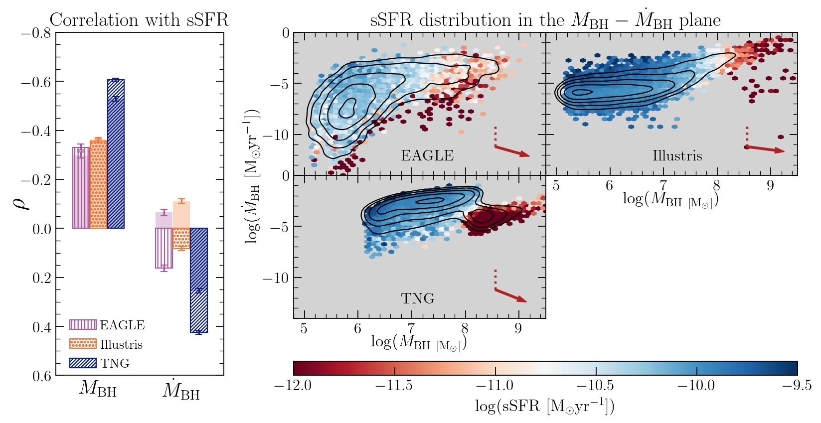
Figure 7: Left: Spearman’s rank correlation coefficient $\rho_{\rm S}$ (full bars) and partial correlation coefficient $\rho_{\rm pcc}$ (hatched bars) between sSFR, ${M_{\rm BH}}$ and ${\dot{M}_{\rm BH}}$. It is apparent that ${\dot{M}_{\rm BH}}$ anti-correlates with quenching in the simulations once its dependence on ${M_{\rm BH}}$ is accounted for. Right: ${M_{\rm BH}}$–${\dot{M}_{\rm BH}}$ plane colour-coded by the median sSFR in a given hexagonal bin. Red arrows indicate the average quenching direction and are oriented at $\theta_{Q}=116^{\circ},\ 103^{\circ}$ and $125^{\circ}$ for EAGLE, Illustris and TNG respectively (see Table 4). Black contours show the density of objects in the plane. In all panels the sSFR gradient changes horizontally or slightly towards the bottom right corner, indicating that quenching requires primarily an increase in ${M_{\rm BH}}$ and a slight decrease in ${\dot{M}_{\rm BH}}$.

4.3.1 $L_{\rm AGN}$ cannot reveal AGN feedback quenching in action

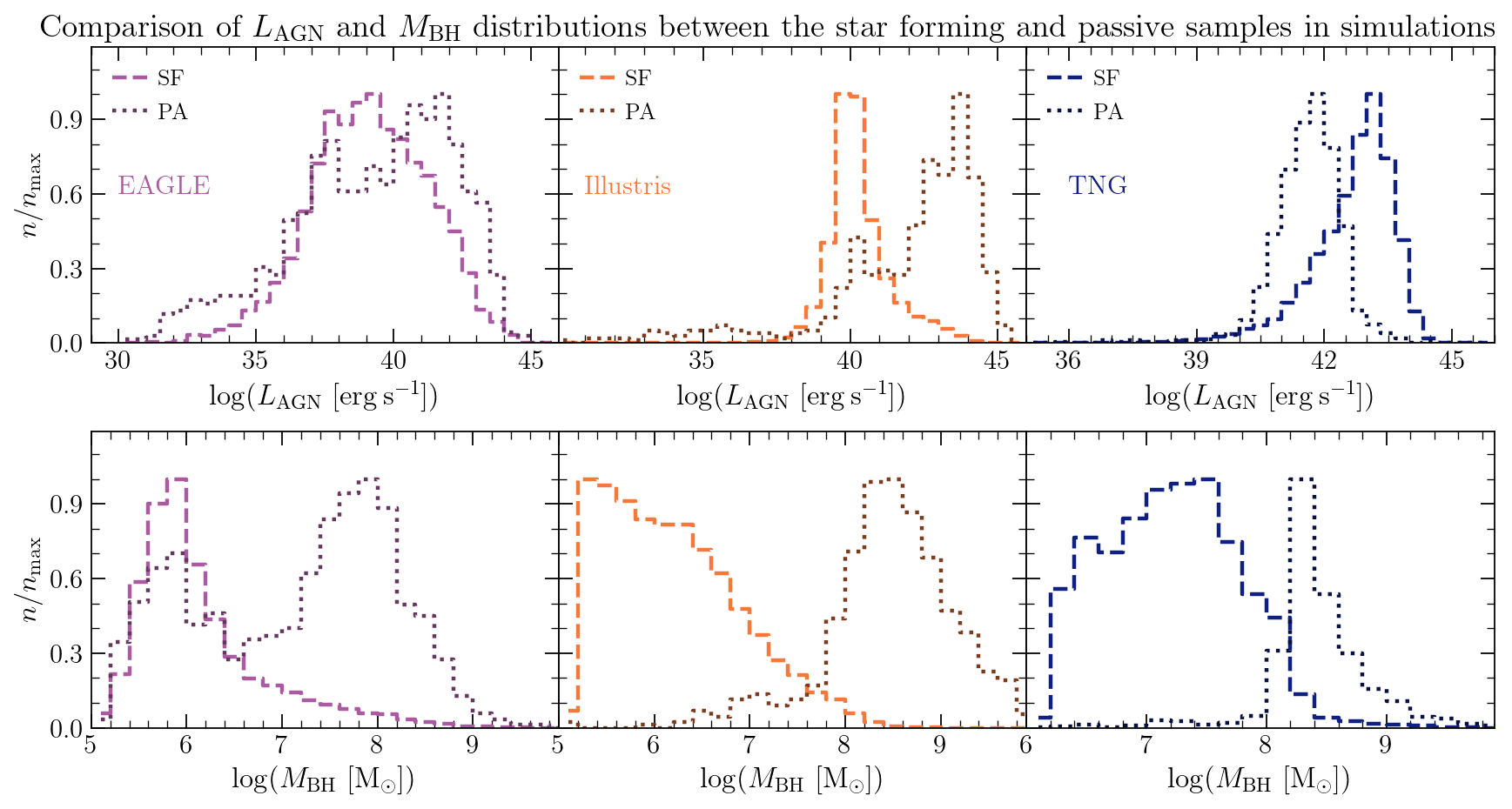
Figure 8: Comparison of distributions in bolometric AGN luminosity (top) and black hole mass (bottom) between the star forming (SF) and passive (PA) galaxy populations in the simulations. All bottom panels show a clear contrast between ${M_{\rm BH}}$ distributions, where PA systems have high ${M_{\rm BH}}$, while their SF counterparts host smaller black holes. In $L_{\rm AGN}$ the picture is different: in TNG higher AGN luminosities are linked to active star formation, Illustris shows an exactly opposite trend, while in EAGLE $L_{\rm AGN}$ is insensitive to the star formation state of the galactic host.

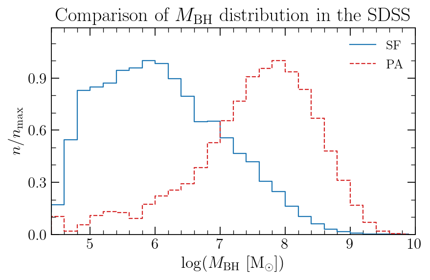
Figure 9: Comparison of black hole mass distributions between the star forming (SF) and passive (PA) galaxy populations in the SDSS. The histograms are weighted to account for the Malmquist bias and the inclination correction. Passive galaxies are clearly associated with more massive black holes than their star-forming counterparts.

We first compare ${M_{\rm BH}}$ against ${\dot{M}_{\rm BH}}$ in Fig. 7. Full bars in the left panel show the Spearman’s rank correlation coefficient between the parameters and sSFR, while the hatched ones present their respective partial correlation coefficients, evaluated at fixed values of the remaining parameter. Please note that the vertical axis is inverted such that upright bars reflect a positive correlation with quenching (a negative correlation with sSFR). At first glance, Fig. 7 informs us about little to no measurable association between the current instantaneous accretion rate of a black hole and the quenching stage of its galactic host. It is also apparent in all simulations that once the connection between ${\dot{M}_{\rm BH}}$ and ${M_{\rm BH}}$ is accounted for, an increased accretion rate at given black hole mass is associated with an increase in sSFR, pointing towards a co-fuelling scenario in which star formation and black hole growth coincide in time.

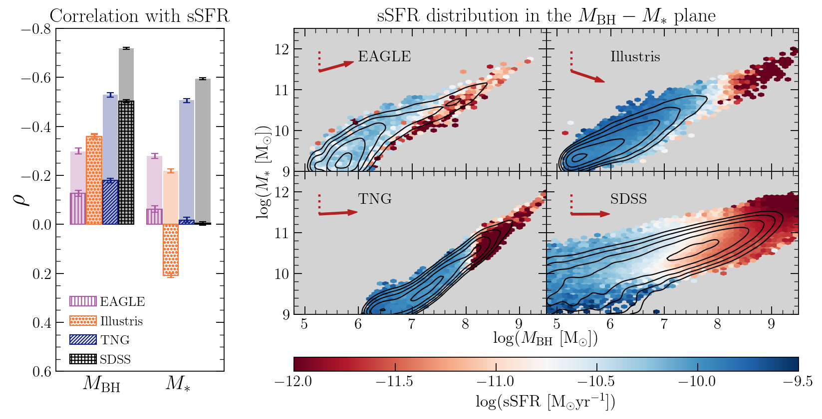
Figure 10: Identical in structure to Fig. 7 but with ${M_{\ast}}$ replacing ${\dot{M}_{\rm BH}}$. Left: The hatched bars demonstrate that ${M_{\ast}}$ is barely associated with quenching once the ${M_{\rm BH}}$–${M_{\ast}}$ relationship is controlled for in the partial correlation. Right: The gradient in sSFR is primarily horizontal in all panels, illustrating that ${M_{\rm BH}}$ is more fundamentally linked to quenching than ${M_{\ast}}$ in both observations and simulations.

In the right panel of Fig. 7 we show the distribution of galaxies in the $M_{\rm BH}-\dot{M}_{\rm BH}$ plane, colour-coded by sSFR. In all three panels a negative gradient in sSFR is primarily driven by an increase in ${M_{\rm BH}}$ and, to a lesser extent, by a decrease in ${\dot{M}_{\rm BH}}$. In Illustris and TNG low sSFRs are associated exclusively with high black hole masses, while in EAGLE there exists a small population of low-${M_{\rm BH}}$ quenched galaxies. The qualitative interpretation of sSFR gradients is confirmed by $\theta_{\rm Q}$ values of $116.2^{+1.4}_{-1.3}$ in EAGLE, $103.0^{+1.2}_{-1.1}$ in Illustris and $125.0^{+0.5}_{-0.5}$ in TNG, which orient all quenching vectors towards the bottom right corners of their respective plots. It is important to point out, however, that $\theta_{\rm Q}$ values are much closer to $\theta_{\rm Q}=90^{\circ}$ than $\theta_{\rm Q}=180^{\circ}$, quantitatively supporting the dominance of ${M_{\rm BH}}$ over ${\dot{M}_{\rm BH}}$  as seen previously in the RF experiment.

To better understand the observable consequences of AGN feedback we show $L_{\rm AGN}$ and ${M_{\rm BH}}$ distributions for passive (PA) and star forming (SF) galaxies in Fig. 8. We estimate AGN luminosities from the black hole accretion rates via $L_{\rm AGN}=\eta c^{2}\dot{M}_{\rm BH}$, where we take $\eta=0.1$, which is a value commonly accepted in the literature as an average radiative efficiency of AGN in the local Universe (e.g Shankar et al., 2009; Bluck et al., 2011; Davis & Laor, 2011; Wu et al., 2013). We also include ${M_{\rm BH}}$ distributions in the SDSS in Fig. 9, for a comparison with the theoretical predictions.

In the bottom panels of Fig. 8 we see the same pattern repeated in all three simulation suites, which is also present in Fig. 9 in the SDSS. Namely, passive galaxies host more massive black holes than the star forming population, regardless of the subgrid prescription for AGN feedback in the simulations. This feature explains why ${M_{\rm BH}}$ is found to be an efficient route to predicting a star forming/passive classification in the Random Forest.

In the top panels of Fig. 8 the situation is strikingly different, since all three simulations predict different behaviour in $L_{\rm AGN}$. In EAGLE the star forming and quiescent galaxy populations show essentially no difference in the instantaneous AGN activity, as demonstrated by the overlapping $L_{\rm AGN}$ histograms. In Illustris passive galaxies are associated with higher $L_{\rm AGN}$, while TNG presents an entirely opposite trend where SF galaxies host more luminous AGN. The stark contrast between the top and bottom panels in Fig. 8 once again demonstrates how different implementations of AGN feedback lead to a ubiquitous signature in ${M_{\rm BH}}$, while the prediction in ${\dot{M}_{\rm BH}}$ ($L_{\rm AGN}$) is far less clear. As demonstrated in Fig. 9, the SDSS observations match the theoretical prediction in black hole mass, showing a clear separation in ${M_{\rm BH}}$ distribution between the SF an PA galaxy populations. However, the overlap between the two distributions is larger than in the simulations, most likely owing to the uncertainty associated with the ${M_{\rm BH}}$ estimation in the SDSS.

The comparisons we draw between ${M_{\rm BH}}$ and ${\dot{M}_{\rm BH}}$ in Figs. 7, 8 & 9 strengthen our conclusions reached in the RF analysis. The PCC calculation demonstrates how the connection between quenching and black hole accretion rate at redshift $z=0$ is negligible in comparison to the relationship with black hole mass. This statement is true for all three different implementations of AGN feedback in EAGLE, Illustris and TNG, which vary in how much feedback energy is generated by the black holes and how that energy couples to their environment. This variation in subgrid prescriptions leaves an imprint on the $L_{\rm AGN}$ distributions, visibly separating the models based on this observable. Most importantly, however, we need to remember that all these simulations quench their central galaxies solely via the AGN feedback. Hence, our results demonstrate that a dependence of quenching on the instantaneous accretion rate at $z=0$ is not a necessary consequence of AGN quenching. In contrast, the strong dependence on ${M_{\rm BH}}$ is necessary, given the ubiquitousness of this trend in three very different simulations.

4.3.2 Connection to black hole mass drives high correlation with quiescence in ${M_{\rm halo}}$ and ${M_{\ast}}$

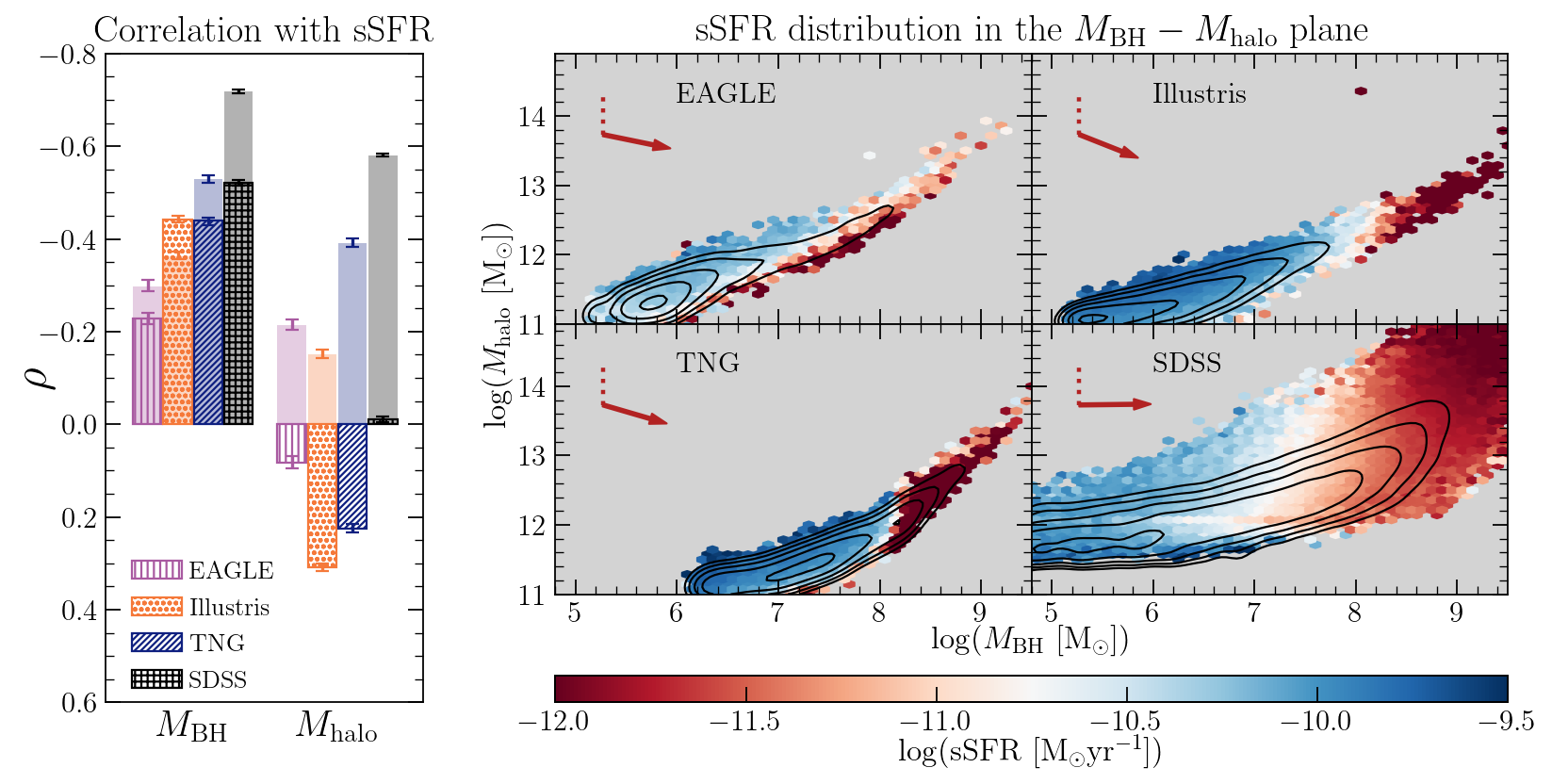
Figure 11: Identical in structure to Fig. 7 but with ${M_{\rm halo}}$ replacing ${\dot{M}_{\rm BH}}$. Left: Hatched bars show that more massive halos result in more star formation once the correlation between ${M_{\rm BH}}$ and ${M_{\rm halo}}$ is taken into account in simulations. In the SDSS the result is consistent with no correlation, rendering the intrinsic connection between sSFR and ${M_{\rm halo}}$ negligible once the inter-correlation with ${M_{\rm BH}}$ is controlled for. Right: the sSFR gradient points towards the bottom right corner in simulations and horizontally in the SDSS, indicating that ${M_{\rm BH}}$ and not ${M_{\rm halo}}$ is the fundamental quenching parameter.

In Fig. 10 we present a comparison between ${M_{\rm BH}}$ and ${M_{\ast}}$, following the structure previously seen in Fig. 7. When we calculate the Spearman’s rank correlation coefficient between sSFR and both ${M_{\rm BH}}$ and ${M_{\ast}}$, we obtain similarly high correlation values for both parameters in all data sets. However, when we account for the ${M_{\ast}}$–${M_{\rm BH}}$ connection, the sSFR-${M_{\rm BH}}$ correlation remains relatively high, while the sSFR-${M_{\ast}}$ PCC is drastically changed. It becomes negligible in SDSS, EAGLE and TNG, while for Illustris the correlation even changes sign (at fixed ${M_{\rm BH}}$ galaxies are more star-forming with increasing ${M_{\ast}}$ in the suite). This behaviour is highlighted in the parameter plane in the right panel, which shows a negative sSFR gradient primarily driven by an increase in ${M_{\rm BH}}$ across all data sets. Like in the previous case of ${\dot{M}_{\rm BH}}$, the transition is most abrupt in TNG, where all objects beyond $\log(M_{\rm BH}/{\rm M_{\odot}})\sim 8$ have log(sSFR/${\rm yr^{-1}}$) $\sim-11$ and below. Our visual gradient inspection is confirmed by the orientation of the quenching vectors, which point at $\theta_{\rm Q}\sim 90^{\circ}$ in SDSS and TNG and within $\pm 45^{\circ}$ from $\theta_{\rm Q}=90^{\circ}$ in Illustris and EAGLE.

This result, together with our previous RF analysis, confirms that the observed connection between galaxy stellar mass and quenching results largely from the black hole-galaxy co-evolution, rather than from quenching being a function of the stellar mass of the system (e.g. due to supernova feedback). Quiescence in massive centrals is primarily caused by the black holes in simulations and hence ${M_{\rm BH}}$ is the parameter determining whether a given galaxy is likely to be quenched. This result is identical to that found by Bluck et al. (2016) for SDSS and Illustris with the use of area statistics in quenched fraction calculations. In this work we update the methodology by using different statistical tests in tandem with machine learning analysis, as well as exploring a broader range of theoretical predictions by including EAGLE and TNG in our investigations.

Finally, we show a comparison between ${M_{\rm BH}}$ and ${M_{\rm halo}}$ in Fig. 11. Like in the case of ${M_{\ast}}$, both parameters are similarly strongly correlated with sSFR, however the difference in $\rho_{\rm S}$ is more pronounced, in favour of black hole mass. When we account for the ${M_{\rm halo}}$–${M_{\rm BH}}$ connection, the correlation changes sign in all simulations and almost vanishes in the SDSS. This implies that at a fixed black hole mass, increasing the dark matter halo mass contributes to an increase in star formation activity of a galaxy in the simulations. This is likely a consequence of higher cooling rates associated with more massive haloes - the original ‘problem’ mitigated by AGN feedback which is still present as a secondary effect, once the primary role of black holes is accounted for. In this scenario increasing halo mass acts to resist quenching rather than aiding it - hence the virial shocks are not effective at keeping halo gas hot and buoyant.

In the observations our result suggest no contribution from ${M_{\rm halo}}$ to quenching, however a weak trend in agreement with the simulations is found in the SDSS by Bluck et al. (2020a). The difference between this work and our analysis is in the use of $\Delta{\rm sSFR}$ in Bluck et al. (2020a) instead of sSFR for the correlation calculations. Nonetheless this does not influence our main conclusion that ${M_{\rm BH}}$ is overwhelmingly more important than ${M_{\rm halo}}$ for the intrinsic galaxy quenching in the observed Universe, in agreement with cosmological simulations and this prior study.

The dominance of ${M_{\rm BH}}$ over ${M_{\rm halo}}$ is further demonstrated in the parameter plane, where the negative gradient in sSFR is, on average, pointing towards the bottom right corner in all simulation panels. In the SDSS the gradient appears more horizontal with a hint of increase in sSFR for increasing ${M_{\rm halo}}$ at fixed ${M_{\rm BH}}$. These qualitative observations are supported by the calculated orientation of the quenching vectors, which have $\theta_{\rm Q}\in(90^{\circ},135^{\circ})$ in all simulations. In the SDSS the arrow is almost precisely aligned with the $x$-axis, i.e. $\theta_{\rm Q}\approx 90^{\circ}$.

The conclusions we draw from Fig. 11, together with the RF analysis, reject one potential halo heating mechanism, which was proposed as a means to quench massive central galaxies. This solution assumes that cold flows in massive haloes (${M_{\rm halo}}$$\gtrsim 10^{12}{\rm M}_{\odot}$) would experience shocks as they fall through the deep halo potential wells. They would then heat up and prevent cooling required for future star formation in a process dubbed virial shock heating (Dekel & Birnboim, 2006). In such a scenario cold gas supply would be ceased for halo masses above a critical shock mass and hence ${M_{\rm halo}}$ could serve as an excellent classification criterion for quenched galaxy population. This is not the case according to our RF results, where the importance of ${M_{\rm halo}}$ is dwarfed by ${M_{\rm BH}}$. Similarly, one would expect halo mass to completely determine the quenching state of a galaxy at fixed black hole mass, meanwhile our partial correlation analysis demonstrates that the opposite behaviour is the case, i.e. that there is a very strong dependence of quenching on ${M_{\rm BH}}$ at fixed ${M_{\rm halo}}$. This result is most pronounced in the SDSS, where the ${M_{\rm halo}}$ $\rho_{\rm pcc}$ almost vanishes.

In all three simulations the PCC result suggests that at a fixed black hole mass more massive haloes experience elevated levels of star formation. This relationship could be potentially explained by increased Bremsstrahlung cooling rates in denser gas, whose density increases with increasing halo mass (Fabian, 2012). Therefore we conclude that both in simulations and observations virial shock heating does not appear to be a viable quenching mechanism in massive central galaxies. With this statement we also confirm the results found previously by Bluck et al. (2016) and Bluck et al. (2020a), reached with different statistical methods for Illustris and the SDSS. More importantly, in this work we investigate theoretical predictions for the partial correlations between ${M_{\rm BH}}$, ${M_{\rm halo}}$ and sSFR in two additional simulation suites: EAGLE & TNG, finding that these are in agreement with trends predicted in Illustris.

In summary, throughout our correlation analysis and RF classification we extract testable predictions for observable consequences of central galaxy quenching in three state-of-the art cosmological simulations. Since EAGLE, Illustris and TNG all quench their centrals using AGN, we effectively test predictions for black hole feedback quenching models against the observed Universe in the SDSS. We find that ${M_{\rm BH}}$ is the most predictive parameter for determining whether a galaxy is quenched or not, both in the simulations and the observations. Hence, so far in this study, we find a close agreement on the predicted observable consequences of AGN feedback among all three simulations, in which the parameter most predictive of quenching in massive centrals is the same, regardless of the implementation of AGN feedback. We also find that ${M_{\rm BH}}$ shows the strongest connection to quenching among all parameters, when explicitly compared with other variables through partial correlations. The vanishing PCCs between sSFR, ${M_{\rm halo}}$ and ${M_{\ast}}$ suggest that the transition to quiescence is not strongly influenced by virial shocks or supernovae, both in the simulations and observations. Most strikingly, however, we learn that cosmological simulations unanimously predict a weak dependence of quenching on redshift $z=0$ ${\dot{M}_{\rm BH}}$, in contrast with its strong connection with ${M_{\rm BH}}$.

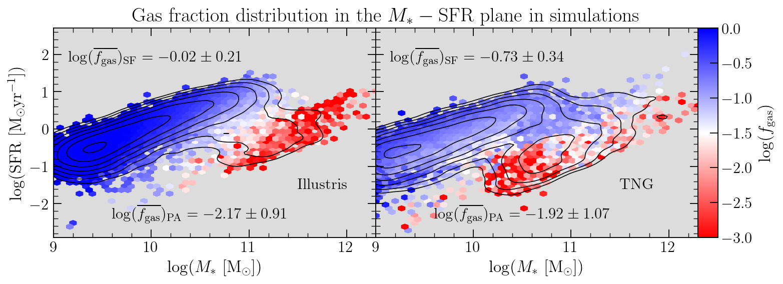
(a) raw result in the simulations

(b) simulations with added observational realism

Figure 12: Comparison of $f_{\rm gas}$ distribution in the $M_{\ast}-{\rm SFR}$ plane between simulations and the SDSS. $(\overline{f_{\rm gas}})_{\rm SF}$ and $(\overline{f_{\rm gas}})_{\rm PA}$ are median gas fractions calculated for the star-forming and passive galaxy populations. Black contours show data distribution in the plane and for SDSS they include $\ifrac{1}{V_{\rm max}}$ and inclination corrections. The raw values in (12(a)) show that $f_{\rm gas}$ is lower in passive galaxies for both simulations, however the magnitude of this difference is larger in Illustris. In (12(b)) we mimic the combined effect of fibre apertures, S/N cut on the ${\rm H}\alpha$ emission line and random scatter on all presented observables in the simulations to allow for a fairer comparison with observations. All panels show qualitatively similar trends in $f_{\rm gas}$, which decreases between the star forming and passive populations. However, this transition is more abrupt and spans a broader range of values in simulations than in the SDSS. Adding observational realism to simulated galaxies primarily softens the trend in $f_{\rm gas}$ for Illustris and causes the scatter in the main sequences to increase in both simulation suites.

Table 5: Median differences in $f_{\rm gas}$ and SFE between the PA and SF populations in Figs. 12 & 13 in units of [dex].

	$\log(\overline{f_{\rm gas}})_{\rm PA}-\log(\overline{f_{\rm gas}})_{\rm SF}$	$\log(\overline{\rm SFE})_{\rm PA}-\log(\overline{\rm SFE})_{\rm SF}$
SDSS	$-0.52\pm 0.44$	$-1.02\pm 0.61$
Illustris raw	$-2.15\pm 0.93$	$0.07\pm 0.84$
Illustris + realism	$-1.40\pm 1.01$	$0.55\pm 0.95$
TNG raw	$-1.19\pm 1.12$	$-1.83\pm 0.38$
TNG + realism	$-2.50\pm 1.03$	$-2.01\pm 0.55$

4.4 Gas content and quenching in the SDSS, Illustris and TNG

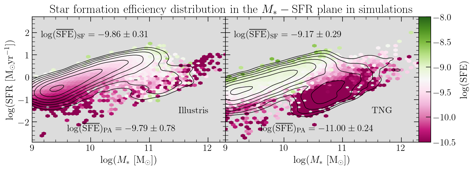
(a) raw result in the simulations

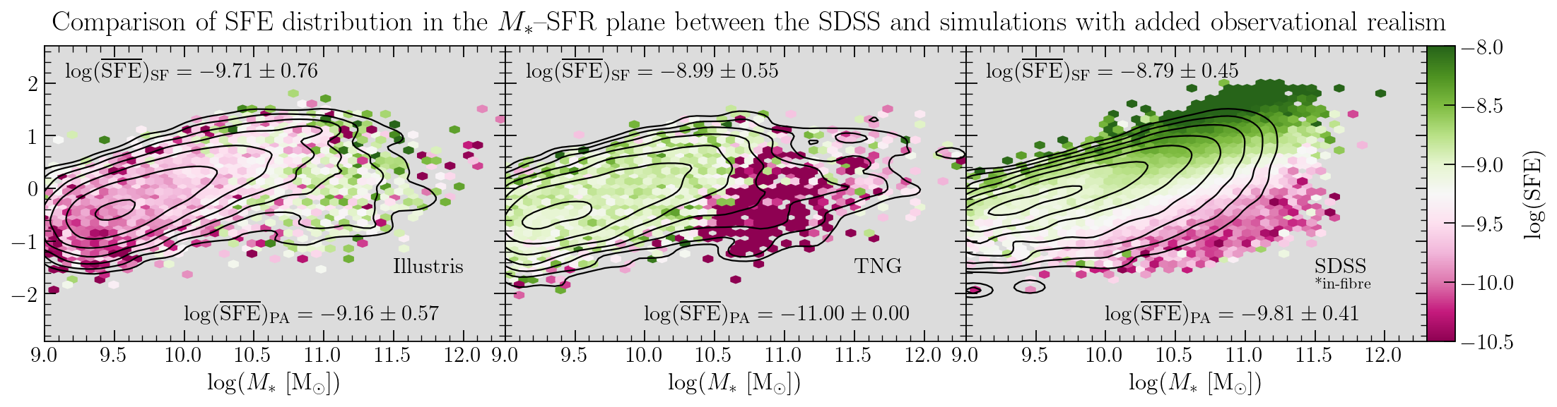
(b) simulations with added observational realism

Figure 13: Analogous to Fig. 12, colour-coded by the median SFE instead of $f_{\rm gas}$. (13(a)) simulations disagree on the change in SFE between the star forming and passive populations. In Illustris star formation efficiency is slightly higher in the quenched objects than on the main sequence, while in TNG the opposite is true. The latter also shows a much more dramatic difference between the star-forming and quenched populations, in which the median SFE drops by almost 2 dex. (13(b)) The addition of observational realism has the effect of further highlighting the opposite trends present in the simulations. In SDSS the SFE mildly increases with increasing mass along the MS and decreases rapidly perpendicular to it. It is apparent that the SFE trend present in TNG agrees qualitatively with the observations, in contrast with Illustris, where it is inverted.

In this section we characterise the potential mode of operation of AGN feedback quenching, looking for its connection to the molecular gas content of galaxies.We focus on Illustris, TNG and SDSS data sets only, omitting EAGLE due to the lack of publicly available molecular gas mass estimates in this suite. We also note that, as highlighted by the quenched fractions and sSFR relations in Sec. 4.1, the quenching trends predicted by EAGLE disagree with those seen in the SDSS, especially at high ${M_{\rm BH}}$. Hence, a detailed investigation of how this AGN feedback mode operates is not strictly necessary in our work. In the SDSS we limit our study to non-AGN dominated galaxies which meet our S/N criteria on emission line fluxes (see Sec. 2.3) in order to reliably estimate ${\rm H}_{2}$ masses from dust reddening of optical spectra. In simulations we check for the potential influence of non-AGN selection by removing objects with ${\dot{M}_{\rm BH}}$ falling in the top 20% of the whole population. We find that this selection does not impact any trends in the simulations, however it significantly depletes the already limited sample of quiescent galaxies in Illustris.

In our analysis we focus on two quantities of interest - molecular gas fraction $(f_{\rm gas}=M_{\rm H2}/M_{\ast})$ and star formation efficiency (${\rm SFE}=\ifrac{\rm SFR}{M_{\rm H2}}$). Multiplied together, these two yield the specific star formation rate of a galaxy:

$${\rm sSFR}=\ifrac{\rm SFR}{M_{\ast}}=\ifrac{M_{\rm H2}}{M_{\ast}}\times\ifrac{\rm SFR}{M_{\rm H2}}=f_{\rm gas}\times{\rm SFE}$$ (22)

and hence allow us to decompose the reduction in sSFR, i.e. quenching, into fuel-driven and and efficiency-driven evolution. In order to decrease $f_{\rm gas}$ one needs to invoke processes which act to reduce molecular gas reservoirs, like e.g. removal through AGN-driven outflows or heating of the CGM to prevent replenishment. Conversely, in order to lower the SFE (or, equivalently, increase the molecular gas depletion time $\tau_{\rm dep}=\ifrac{1}{\rm SFE}$) one can imagine a mechanism which does not affect the amount of gas but rather reduces the efficiency with which it collapses to form new stars, like e.g. injection of turbulence into the ISM (e.g. Krumholz & McKee, 2005).

By examining the changes in $f_{\rm gas}$ and SFE we can thus characterise the observational consequences of different AGN feedback modes as implemented in Illustris and TNG. A fair comparison between predicted trends and those observed in the SDSS can then inform us about the potential physical mechanisms responsible for quenching in the observed Universe and highlight potential areas for improvement in the implemented models.

4.4.1 A universal trend: gas fractions decrease with increasing black hole mass

In Fig. 12 we present the evolution $f_{\rm gas}$ across the $M_{\ast}-{\rm SFR}$ plane in the simulations and observations. Galaxies are grouped into hexagonal bins in the plane and each bin is colour-coded by its median $f_{\rm gas}$, while black contours indicate the density of objects in each panel. The SDSS contours include $\ifrac{1}{V_{\rm max}}$ and inclination corrections. The figure also lists the median $f_{\rm gas}$ in the passive and star-forming galaxy populations labelled as $(\overline{f_{\rm gas}})_{\rm PA}$ and $(\overline{f_{\rm gas}})_{\rm SF}$ respectively. Analogously to Fig. 2 very low SFR objects are redistributed to locations corresponding to upper limits on SFR from Brinchmann et al. (2004), in order for us to present all simulated galaxies in the plane. We would also like to remind the reader that all results presented in Sec. 4.4 use the Gnedin & Draine (2014) model for the HI/H2 transition, out of the four models made publicly available by the Illustris and TNG teams. Although we find differences in the ${\rm H_{2}}$ content on a galaxy-by-galaxy basis, the statistical behaviour of the galaxy population is not affected by our choice of transition model. We further describe the models and show the robustness of our result to this choice in Appendix E.

In Fig. 12(a) we focus on the raw result in the simulations first, characterising a theoretical prediction for idealised molecular gas observations covering the whole spatial extent of galaxies. Both panels in Fig. 12(a) show a clear bimodality in colour, where star forming (SF) galaxies are associated with higher gas fractions than their passive (PA) counterparts. These differences are most striking in Illustris, as highlighted by the colour ranges and median change in $f_{\rm gas}$ of 2.15 dex between the populations. This suite also shows a decreasing trend in $f_{\rm gas}$ with increasing ${M_{\ast}}$ across the MS, which is very mild in comparison with the drop in $f_{\rm gas}$ away from the MS. TNG shows similar qualitative trends in a narrower range of values with a median difference between populations of 1.19 dex. The passive sequence also shows significant scatter in $f_{\rm gas}$ at high ${M_{\ast}}$, in part driven by low sample statistics. Overall, we note that the two simulations are in good qualitative agreement with each other but that Illustris exhibits a steeper declining trend in gas fraction between the star forming and passive galaxy populations.

Table 6: Standard deviation $\sigma_{X}$ of random error in quantity $X$ in the SDSS.

$X$	$M_{\rm\ast,tot}$	$M_{\rm\ast,fib}$	${\rm SFR}_{\rm tot}$	${\rm SFR}_{\rm fib}$	$M_{\rm H2}$	${M_{\rm halo}}$	${M_{\rm BH}}$
$\sigma_{X}$	0.15	0.10	0.30	0.30	0.40	0.50	0.50

In Fig. 12(b) we compare the distribution of $f_{\rm gas}$ in the simulations against the SDSS. In order to bring all data sets to a comparable footing, we apply several layers of observational realism to galaxies in Illustris and TNG. As we explain in detail in Appendix D, we mimic the effect of an SDSS fibre aperture by focusing on central regions in the galaxies and integrating $M_{\rm H2}$, ${M_{\ast}}$ and SFR profiles up to their assigned fibre radii. Depending on the simulated galaxy mass, such mock fibre radius is randomly drawn from a distribution of physical fibre sizes seen in a given stellar mass bin in the SDSS. We also imitate the way in which emission line quality cuts influence the observed sample by removing a number of simulated galaxies with low SFRs. Removed objects are chosen at random from the SFR distribution in the simulations, such that the fraction of galaxies remaining in a given SFR bin traces the SDSS sample completeness as function of SFR after imposing the emission line S/N cuts. Finally, we also account for the random measurement errors in all quantities of interest by adding random Gaussian noise to their values drawn from the simulations. In this step, previously described for quenched fractions in Section 4.1, for each quantity $X$ among the in-fibre ${M_{\ast}}$, SFR and $M_{\rm H2}$, a given simulated galaxy is assigned $X_{\rm new}$ with $\log(X_{\rm new})=\log(X)+N(0,\sigma_{X})$. The values of $\sigma_{X}$ are dictated by random error distributions in the SDSS and are listed in Table 6 for all relevant quantities. All observational realism steps along with their influence on the results in Fig. 12(a) are described in detail in Appendix D.

Fig. 12(b) shows some common trends present in both simulations with added observational realism and the SDSS. Across all three panels, main sequence galaxies have higher gas fractions than their quenched counterparts, with simulations showing significantly more dramatic difference in median $f_{\rm gas}$ between the two populations. In the SDSS this variation amounts to only 0.52 dex and includes all sample corrections in the calculation. We can also see a slightly decreasing trend in $f_{\rm gas}$ with increasing ${M_{\ast}}$ across the MS in all panels, which is significantly milder than the evolution between MS and the passive sequence.

Apart from these similarities, Fig. 12(b) also shows a range of differences between both simulation suites and the SDSS. While in the observations the lowest gas fractions are only found in galaxies with the most extreme deviations away from the Main Sequence, in both simulations these extreme values of $f_{\rm gas}$ are distributed across the entire passive sequence. This trend is slightly more extreme in TNG, where the galactic centres of quenched galaxies are almost exclusively gas-poor. It is also important to note that the gradient in $f_{\rm gas}$ in the SDSS is approximately perpendicular to the MS, while in both simulation suites it points almost horizontally with an abrupt drop in $f_{\rm gas}$ above $\sim 10^{10.8}{\rm M_{\odot}}$ in Illustris and $\sim 10^{10.5}{\rm M_{\odot}}$ in TNG. In TNG this dramatic change appears around a threshold mass for which the AGN feedback mode switches from thermal to kinetic (Weinberger et al., 2017).

Despite the addition of random scatter in Illustris and TNG, the observations still cover the largest area in the $M_{\ast}-{\rm SFR}$ parameter space and show the smoothest evolution in $f_{\rm gas}$ across the plane. The shortage of simulated galaxies in the passive cloud is highlighted even further by the imitation of S/N cut on emission lines, with only a handful of objects left to compare with the SDSS. The observed and simulated main sequences also differ, with the SDSS contours showing a much tighter relation than those seen in Illustris and TNG. This comparison suggests that the emerging MS relations in the simulations are potentially too broad, given that the width of the SDSS Main Sequence can be attributed to measurement uncertainties to a large extent. However, we do recognise that our treatment of measurement uncertainties in simulated quantities is rather simplistic and hence we only point out this MS feature as a hint of a potentially interesting result. An accurate translation between simulated observables and their realistic measurement requires careful consideration of the electromagnetic radiation emitted by galaxies, which is beyond the scope of this work.

Fig. 12(a) indicates that one potential impact black holes have on their galactic hosts is depleting dense gas available for star formation. This is demonstrated by the dramatic decrease in $f_{\rm gas}$ between the star forming and passive galaxy populations drawn from the simulations. When we post-process the simulations with observational realism and compare them against the SDSS in Fig. 12(b), we find a qualitative agreement across all panels, albeit the range of values we see in observations is more modest (see Table 5 for a As we point out earlier, the trends are also more dramatic in the simulations than the observations, suggesting that although cosmological simulations successfully recover the large-scale effects quenching has on galaxy populations, the details of its implementation still leave room for further improvement.

These results suggest that our current observations of molecular gas content of local, massive central galaxies can potentially be explained by AGN acting to prevent the re-supply of fuel for future star formation. In Illustris and TNG, AGN achieve this primarily by preventing the accretion of new gas from hot galactic haloes. However, based on our comparison alone, we cannot reject the potential involvement of ejective forms of AGN feedback which would lead to similar observational signatures and be particularly relevant for the lower end of our investigated stellar mass range.

4.4.2 Conflicting trends in star formation efficiency

In Fig. 13 we explore how star formation efficiency (${\rm SFE}=\ifrac{\rm SFR}{M_{\rm H2}}$) changes across the $M_{\ast}-{\rm SFR}$ plane. Analogously to Sec. 4.4.1 we analyse the ‘raw’ result first and then add simulation realism to compare the simulations with the SDSS. In all panels, objects with ${\rm SFR}=0$ in the simulations are assigned a nominal low value of log(SFE/${\rm yr^{-1}}$) $=-11$ and hexagonal bins dominated by these objects saturate the colour scale with dark magenta.

In Fig. 13(a) Illustris and TNG do not agree on the trends in SFE, in contrast with the previously seen $f_{\rm gas}$ distributions. Illustris galaxies have slightly higher SFEs in the bulk of the passive sequence, with a median increase of only 0.07 dex when compared to SF objects. The passive sequence in Illustris is also subject to variation owing to small number statistics. In contrast, TNG experiences a dramatic drop in median SFE of 1.83 dex and its passive sequence is dominated by objects with ${\rm SFR}=0$. These are redistributed to higher sSFR values to allow a visual comparison in the $M_{\ast}-{\rm SFR}$ plane and are assigned a nominal low value for SFE of $10^{-11}{\rm yr^{-1}}$.

In Fig. 13(b) we apply observational realism to the simulations (see appendix D) and compare them against the SDSS. Adding observational realism results, on average, in higher SFE values in both simulation suites. This is a combined effect of removing low-sSFR simulated galaxies to mimic S/N ratio cut in the SDSS and restricting galaxies to their centres, which are more efficient at forming stars than the outskirts. When we then focus on observations, we find a slight increase in SFE with increasing ${M_{\ast}}$ on the Main Sequence along with a dramatic decrease of almost 2 dex in the direction perpendicular to the MS. The evolution of SFE in the SDSS is smooth and only shows pronounced scatter around the edge of the passive sequence owing to low number statistics. These general trends are not well reproduced in the simulations and hence all three panels show visible differences among each other. In Illustris the direction of the trend is essentially inverted, such that MS values of SFE are approximately 0.6 dex lower than those seen in the scarcely populated passive sequence. In TNG, although the quenched population shows lower SFE values than the MS, this change is significantly more abrupt than observed in the SDSS. Similarly to the trends seen in $f_{\rm gas}$, the simulations show steeper gradients in SFE than the observations, which primarily point in the horizontal direction, rather than perpendicular to the Main Sequence. Nonetheless, adding observational realism once again has the effect of strengthening the trends visible in the raw simulation data, in this case amplifying the contrast between Illustris and TNG.

Our analysis of Fig. 13(a) demonstrates that different models predict contrasting behaviour in star formation efficiency in the $M_{\ast}-{\rm SFR}$ plane. Both Illustris and TNG quench their massive centrals primarily via AGN feedback, however it is apparent in the colour gradients that the two suites predict two opposing trends in SFE. Interestingly, neither of the results is exactly reflected in the observations when we compare them against the SDSS in Fig. 13(b). Adding observational realism further highlights the juxtaposition of Illustris and TNG, yielding a bimodal distribution in SFE between passive and star forming galaxies in both suites. Between the two theoretical predictions, there seems to be no model clearly favoured by the observed Universe. However, given the trends seen in the SDSS, we would expect a successful prediction to recover a significant decrease in both $f_{\rm gas}$ and SFE in a direction perpendicular to the Main Sequence.

4.5 The dependence of $f_{\rm gas}$ and SFE on ${M_{\rm BH}}$

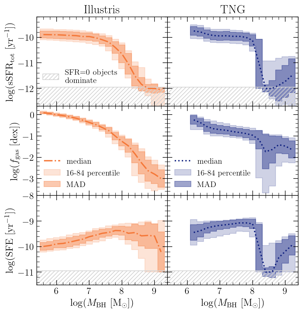
Figure 14: Median sSFR (top row), gas fraction (middle row) and SFE (bottom row) as function of ${M_{\rm BH}}$ in Illustris and TNG. Gray hatched regions indicate where the results are dominated by galaxies with SFR=0. Both simulations agree on the trends in sSFR and $f_{\rm gas}$, where both quantities decrease with increasing ${M_{\rm BH}}$. The variation in sSFR is more dramatic in TNG, showing a sharp drop around $\log(M_{\rm BH})\sim 8.1$. In $f_{\rm gas}$ Illustris galaxies show a broader range in values, spanning 3 dex in logarithmic units. Simulations disagree about the behaviour of SFE, which steadily increases with ${M_{\rm BH}}$ in Illustris, while in TNG is initially roughly constant and drops off dramatically at high black hole masses.

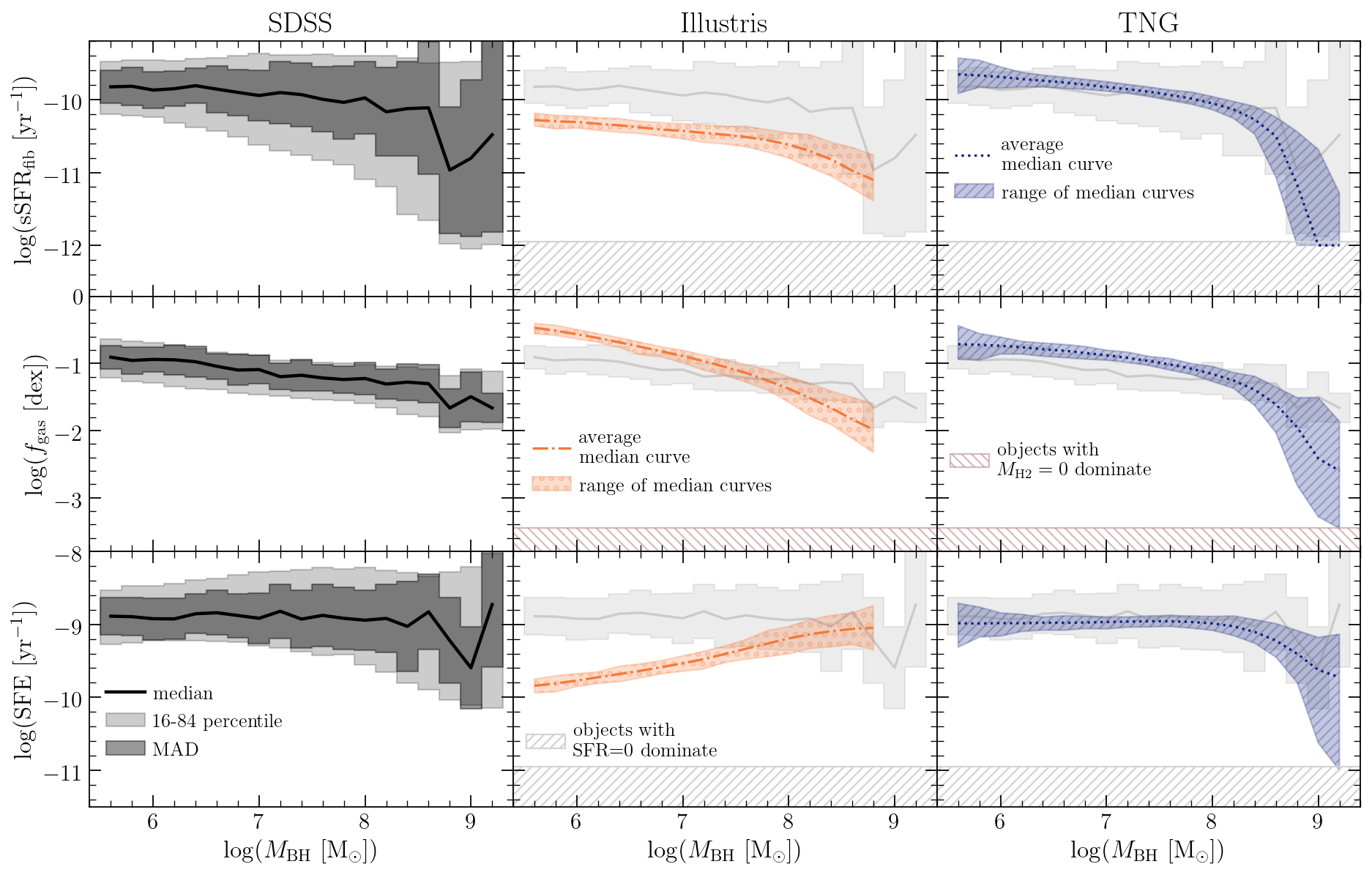
Figure 15: Median sSFR (top row), gas fraction (middle row) and SFE (bottom row) as function of ${M_{\rm BH}}$ for SDSS, Illustris and TNG (left to right panels respectively). In observations, all quantities are obtained from fibre spectroscopic measurements and the sample is restricted to galaxies with visible emission line signal. The simulation panels differ from raw results in Fig. 14 due to the application of observational realism described in appendix D. The SDSS curves include $1/V_{\rm max}$ and inclination corrections placing all panels on equal footing. Both simulations show decreasing trends in ${\rm sSFR_{fib}}$ and $f_{\rm gas}$ in line with the observations, however TNG is a better quantitative match with the SDSS. SFE in the observations shows a mild decrease at the highest ${M_{\rm BH}}$ and a similar trend is visible in TNG. The curves in Illustris show an opposite behaviour, increasing SFE with increasing ${M_{\rm BH}}$, which is clearly discrepant with the observations.

In the final part of our analysis we look directly at possible connections between ${M_{\rm BH}}$ and molecular gas content of galaxies to further investigate the mode of operation of AGN feedback quenching. We first analyse the simulations only and proceed by splitting the samples into 0.2 dex wide bins in ${M_{\rm BH}}$ to calculate median values of sSFR, $f_{\rm gas}$ and SFE in each bin. We plot the curves resulting from this calculation as dotted and dash-dotted lines in Fig. 14, indicating the median absolute deviation (MAD) and the 16-84 percentile range of values in a given bin with shaded regions. In order to include all galaxies with ${\rm SFR}=0$, we assign them nominally low values for both sSFR and SFE of log(sSFR/${\rm yr^{-1}}$) $=-12$ and log(SFE/${\rm yr^{-1}}$) $=-11$, respectively. Gray hatched regions in the top and bottom panel rows indicate bins dominated by the SFR=0 objects, which occur for $10^{8.2}{\rm M_{\odot}}\lesssim M_{\rm BH}\lesssim 10^{8.6}{\rm M_{\odot}}$ in TNG and $M_{\rm BH}\gtrsim 10^{8.8}{\rm M_{\odot}}$ in Illustris.

In the top two rows in Fig. 14 we see a qualitative agreement between the trends in Illustris and TNG. Central galaxies in both simulations experience decreasing sSFR and $f_{\rm gas}$ as a function of increasing ${M_{\rm BH}}$. In Illustris the change in sSFR is more gradual, while in TNG it resembles a step function around a characteristic black hole mass of $\log(M_{\rm BH}/{\rm M_{\odot}})\sim 8$, where the AGN feedback mode changes from ‘quasar’ to ‘kinetic’ (Zinger et al., 2020). The gas fraction curve in TNG also shows a visible dip around the same characteristic ${M_{\rm BH}}$, while in Illustris it is a smooth decreasing trend, spanning $3\ {\rm dex}$ in $f_{\rm gas}$. The SFE curves in the bottom panel show the most difference between the simulations. In TNG the efficiency remains roughly constant for $M_{\rm BH}<10^{8}{\rm M_{\odot}}$ and drops dramatically beyond this critical black hole mass. In Illustris the the SFE behaviour seems to go against TNG – the efficiency rises steadily with increasing ${M_{\rm BH}}$ and then falls off at the highest black hole masses, where the data shows significant scatter due to low number statistics.

In Fig. 15 we take these theoretical predictions, add observational realism and compare the final results with the SDSS. The observed sample is restricted to objects with reliable emission line measurements according to the selection criteria in Section 2.3 and the calculated curves are weighted to correct for the Malmquist bias and the cut on disk inclination. The coloured shaded regions in the simulations show a range of median curves resulting from 500 random realisations of adding measurement error to the raw data post-processed to reflect aperture correction and emission line S/N ratio cuts. In the process of mimicking an SDSS fibre aperture in the simulations we arrive at a population of galaxies which have $M_{\rm H2}=0$ and assign them with a nominal low gas fraction value of $\log(f_{\rm gas})=-3.5$. All objects with both $M_{\rm H2}=0$ and SFR=0 are removed from the calculations since their value of SFE is mathematically ambiguous (without the knowledge of the functional forms of ${\rm SFR}(M_{\rm BH})$ and $M_{\rm H2}(M_{\rm BH})$ we are unable to determine the finite value of the otherwise undefined SFE in the limit). Hatched rectangular regions in Fig. 15 indicate where objects devoid of star formation (gray hatch) and molecular gas (brown hatch) dominate.

We first look at the in-fibre sSFR (${\rm sSFR_{fib}}$) in the top left corner in Fig. 15. The decrease towards low sSFR values in the fibre occurs at significantly higher ${M_{\rm BH}}$ than we previously saw in the case of total sSFR. This is a direct result of the emission line S/N ratio cuts biasing the sample towards more star-forming systems. The shaded regions are also visibly broader than before, owing to a fivefold decrease in sample size. This dramatic change between the in-fibre and total result illustrates how critical it is to apply similar selection criteria to both the simulations and observations for a successful comparative analysis. Standard procedures necessary in the observations (e.g. emission line quality cuts or restricting the field of view to galactic centres) need to be applied to theoretical predictions in order to ensure a fair comparison between the models and the observed Universe.

Both simulations in Fig. 15 show a decreasing trend in the aperture-restricted sSFR, qualitatively consistent with the observations. TNG shows a better quantitative match, tracing the SDSS curve reasonably well across the entire range in ${M_{\rm BH}}$. Gas fraction in the middle row of Fig. 15 shows a significant, steady decline of $\sim 1\ {\rm dex}$ in the SDSS. Similarly to sSFR, both simulation suites predict trends qualitatively similar to the observations. Galaxies with low ${M_{\rm BH}}$ in Illustris have higher initial $f_{\rm gas}$ than the observations, which then decreases more rapidly to become lower than in the SDSS at highest ${M_{\rm BH}}$. The $f_{\rm gas}$ curve in TNG traces the SDSS median values within their MADs until $M_{\rm BH}\sim 10^{8.4}{\rm M_{\odot}}$, where it rapidly drops to values around 1 dex lower than the SDSS.

The most striking result presented in Fig. 15 is the comparison of star formation efficiency trends in the bottom row. In the SDSS, the SFE remains approximately constant until $M_{\rm BH}\sim 10^{8.5}{\rm M_{\odot}}$, where it falls off by a total of 0.5 dex to then pick up in the highest ${M_{\rm BH}}$ bin. Galaxies in Illustris show a different trend, where their median SFE rises by 1 dex with increasing ${M_{\rm BH}}$ to reach the initial SDSS value of ${\rm SFE}\approx 10^{-9}{\rm yr^{-1}}$ at $M_{\rm BH}\sim 10^{8.8}{\rm M_{\odot}}$. In contrast, TNG seems to follow the SDSS curve across a broad range in black hole mass, with the exception of the highest ${M_{\rm BH}}$ bin.

Comparing Figs. 14 & 15 allows us to characterise the impact of adding observational realism on the inferred theoretical predictions. Across all three variables: sSFR, $f_{\rm gas}$ and SFE mimicking measurement uncertainty smoothens the gradients present in both simulations. It is particularly visible in TNG, where the step function behaviour is removed from the curves. The aperture correction in Illustris acts to reduce sSFR and $f_{\rm gas}$, and to increase SFE, primarily at the highest ${M_{\rm BH}}$. In contrast, in TNG galactic centres are more star-forming at low ${M_{\rm BH}}$ and devoid of both gas and star-formation at $\log(M_{\rm BH}/{\rm M_{\odot}})\gtrsim 8$. Finally, mimicking a S/N ratio cut results in removing high-${M_{\rm BH}}$ objects in both simulations, since low SFRs are primarily associated with massive black holes in these two model implementations. Combined together, our post-processing steps primarily act to highlight the raw trends identified earlier in Fig. 14. We see how Illustris and TNG agree on the behaviour of sSFR and $f_{\rm gas}$ as a function of ${M_{\rm BH}}$ and how they clearly disagree on the trends in SFE. For a detailed discussion on the impact of all observational realism steps we refer the interested reader to Appendix D.

Overall, our analysis of molecular gas trends predicted by the simulations shows that neither model perfectly reflects the observed Universe. We note, however, that the SFE trends seen in the SDSS are in a better agreement with those predicted by TNG than Illustris, especially when we consider galactic centres with full observational realism.

5 Discussion

5.1 Quenching modus operandi in massive central galaxies

The result of our Random Forest classification, together with the PCC analysis, clearly indicate that black hole mass is the most successful parameter at determining the quenching state of massive central galaxies at redshift $z=0$. We find this statement about the ${M_{\rm BH}}$ dominance to be true regardless of the detailed implementation of the feedback model in the simulations or the choice of ${M_{\rm BH}}$ calibration in the observations. Throughout this paper we also show that ${M_{\rm BH}}$ is superior to other galactic parameters like ${M_{\rm halo}}$ and ${M_{\ast}}$, a conclusion previously reached with a different statistical approach by Bluck et al. (2016) in the SDSS and in a sample of direct black hole mass measurements in Terrazas et al. (2016, 2017). We improve on these previous works by extending the set of cosmological simulations to EAGLE and IllustrisTNG, enriching our analysis with molecular gas content within the galaxies, as well as using a more sophisticated machine learning based analysis method.

In this work we limit our research to central galaxies in order to characterise the intrinsic quenching mechanisms only. Since centrals reside at the minima of their dark matter halo potentials, we expect the effect of environment on ceasing star formation to be minimal, avoiding e.g. ram pressure stripping of molecular gas (e.g. Peng et al., 2012; Bluck et al., 2016, 2020b). Our results demonstrate that all three cosmological simulations: EAGLE, Illustris and TNG, share a common theoretical prediction for the observable consequences of AGN feedback quenching and that this prediction is met overwhelmingly well in the Universe as observed in the SDSS.

More specifically, we find that the current star formation state of a galaxy is determined by the integrated history of AGN feedback (encoded in ${M_{\rm BH}}$) rather than the instantaneous AGN luminosity at redshift $z\sim 0$ (as inferred from ${\dot{M}_{\rm BH}}$). Our findings confirm conclusions reached for small samples of direct black hole mass and accretion rate measurements in the local Universe (Terrazas et al., 2016, 2017) as well as individual analyses of cosmological simulations (Davies et al., 2019; Terrazas et al., 2020; Zinger et al., 2020). Our study is unique, however, in that it treats all simulations consistently throughout the whole analysis. We apply the same statistical tests and Random Forest classification to reveal a unanimous conclusion in all simulation suites – at redshift $z=0$ ${M_{\rm BH}}$ is the key parameter determining galaxy quiescence, while the instantaneous ${\dot{M}_{\rm BH}}$ holds very little predictive power once its connection to ${M_{\rm BH}}$ is accounted for. The theoretical prediction of ${M_{\rm BH}}$ dominance is also recovered clearly in the SDSS observations, where we subject the data to an identical analysis.

Although the importance of ${M_{\rm BH}}$ and AGN quenching are at the focus of this paper, our analysis delivers a useful discussion of other quenching avenues potentially available to massive central galaxies. Our Random Forest experiment, together with the PCC analysis, show that there indeed exists a connection between quiescence and both ${M_{\ast}}$ and ${M_{\rm halo}}$ individually. However, we interpret these relations as secondary in nature and stemming from the inter-correlations between stellar, halo and black hole mass. Once ${M_{\rm BH}}$ is identified as the most important parameter among ${M_{\rm BH}}$, ${M_{\rm halo}}$ and ${M_{\ast}}$ and its numerical association with stellar and halo mass is accounted for, a picture emerges in which the previously recognised correlations are incidental, rather than intrinsic.

These results neatly illustrate that correlation does not imply causation, regardless of how high the correlation measurement is. By showing how the correlations between sSFR, ${M_{\rm halo}}$ and ${M_{\ast}}$ vanish at a fixed ${M_{\rm BH}}$ we unambiguously demonstrate that these correlations are spurious, i.e. not causal in origin. Hence there is no doubt that more massive galaxies are more likely to be quiescent as demonstrated by e.g. Baldry et al. (2006), Peng et al. (2010) and Peng et al. (2012), however this relationship is primarily a consequence of ${M_{\ast}}$ being tied to ${M_{\rm BH}}$ in the black hole - galaxy co-evolution. Similarly, massive haloes are populated with quenched objects, in agreement with e.g. Woo et al. (2013) and Woo et al. (2015), however it is likely not due to the influence of virial shock heating (as suggested by Dekel & Birnboim, 2006), but rather driven by the connection between the black hole and halo masses.

As a final remark we would like to stress that AGN feedback is unlikely to be the only mechanism responsible for galaxy transition to quiescence in its entirety. In fact, given the wealth of evidence for a connection between quenching and other galactic parameters, as well as the measurement uncertainty associated with all variables of interest, one would expect multiple processes to be at play simultaneously, bringing star formation to a halt together.

A good example of such process would be the occurrence of stabilising torques from the central bulge which could prevent gas from collapsing to form new stars via ‘morphological quenching’ (Martig et al., 2009). This scenario would decrease in the efficiency with which molecular gas is forged into news stars, leading to the observed low SFEs in the SDSS. This mechanism on its own, however, cannot explain the reduced gas fractions experienced by passive galaxies and hence could not be solely responsible for galactic transition to quiescence in the observations. The resolution limit in EAGLE, Illustris and TNG unfortunately does not allow us to investigate the theoretical predictions for morphological quenching potentially working in tandem with AGN feedback. However, recent simulations of idealised galaxies suggest that the presence of a central bulge is associated with decreased star formation activity in models which do not include prescriptions for black hole feedback (Gensior et al., 2020).

5.1.1 How do AGN prevent galaxies from forming stars?

In this work we investigate theoretical predictions for the observable consequences of AGN feedback quenching in three different feedback model implementations. Numerical simulations of galaxy evolution typically divide the interaction of supermassive black holes with their environment into two categories: the thermal, ‘quasar mode’ feedback operating at high accretion rates and the preventative, ‘radio mode’ feedback associated with less efficient accretion (e.g. Bower et al., 2006; Croton et al., 2006; Sijacki et al., 2007; Booth & Schaye, 2011; Vogelsberger et al., 2014a; Somerville & Davé, 2015; Weinberger et al., 2018). In the quasar mode, AGN demonstrate their presence through powerful radiation across the whole electromagnetic spectrum, feeding on cold, dense gas to launch high-velocity winds from the black hole accretion disks (e.g. Crenshaw et al., 2010; Rupke et al., 2017). The radiatively inefficient radio (‘mechanical’) AGN mode, on the other hand, is associated with synchrotron emission from charged particles in AGN jets (e.g. McNamara & Nulsen, 2007; Fabian, 2012). These two modes differ in both the location of energy injection (local vs at large distances) and the method by which this energy is deposited into the gas (radiative vs. mechanical).

The ‘kinetic bubble’ model implemented in Illustris (see Sec. 2.2) is designed to mimic the effect of interactions between AGN jets and the CGM at large distances away from a galaxy. By placing bubbles at random locations within the CGM, AGN in Illustris evacuate the gas residing in galactic haloes and, to a lesser extent, heat up the leftover gas reservoirs. This prescription is extremely efficient at depleting hot gas haloes around massive galaxies, leaving them devoid of fuel for subsequent cooling and future star formation. Although this AGN feedback model successfully quenches central galaxies, it does so by removing hot gas haloes around them. This predicted outcome is inconsistent with observations, which commonly show large quantities of hot, ionised gas surrounding massive centrals (e.g. Fabian, 2012).

AGN feedback at low Eddington ratios in TNG aims to improve on the Illustris design by implementing a kinetic mode, which would keep massive galaxies quenched without stripping their hot gas haloes. This kinetic feedback mode is designed to imitate the potential effect of interaction between the galaxy ISM and AGN winds at small distances around the AGN and proves very successful at preventing excessive gas removal from around the galaxy. By introducing momentum kicks in random directions, the model aims at capturing nucleus-scale interactions which over time percolate outside the galaxy, increasing the entropy of gas in the CGM as well as the ISM. As shown in Terrazas et al. (2020) this kinetic feedback mode also results in cold gas being pushed out of galaxies, since the wind energies exceed the binding energy of gas within the hosts.

When we look at the connection between ${M_{\rm BH}}$ and different galactic properties compared across all simulations and the SDSS, we see that the observations show trends which are not perfectly captured by the theoretical predictions from Illustris and TNG. Nonetheless, our analysis shows promising qualitative agreement between the predicted and observed trends, which seems more pronounced in TNG out of the two simulation suites. It is apparent in Sec. 4.1 that although transition to quiescence happens at higher values of ${M_{\rm BH}}$, ${M_{\rm halo}}$ and ${M_{\ast}}$ than in the SDSS for all simulations, the trends in TNG show a promising resemblance both in terms of slopes and their behaviour in the parameter value limits, once observation-like scatter is added to the data. The EAGLE suite stands out as well, showing the shallowest slopes among all simulations. More importantly, however, quenched fractions in EAGLE point towards insufficient strength of its AGN quenching mechanism, which results in a quenched fraction ceiling of $f_{Q}\sim 0.6$ and a sSFR floor of log(sSFR/${\rm yr^{-1}}$) $\sim-11$ (i.e. barely quenched at all).

The analysis of molecular gas content in Illustris, TNG and the SDSS in Sec. 4.4 allows us to directly compare the effect of two different feedback implementations on the AGN host galaxies. The mechanical bubble model implemented in Illustris successfully removes fuel available for star formation by keeping the halo gas hot and preventing its collapse on the galaxy to replenish cold gas reservoirs. In this fashion, the simulation efficiently shuts down star formation in the outskirts of massive galaxies, leaving behind galactic centres with enough gas to fuel both the central black hole and the star formation in the central region.

We then contrast this picture with TNG, where the preventative feedback in the form of momentum injection around the AGN leads to a more balanced scenario. In a fashion similar to that seen in the SDSS, both SFE and $f_{\rm gas}$ decrease, together resulting in decreasing sSFR with increasing ${M_{\rm BH}}$. The efficiency is mostly insensitive to the change in black hole mass until around $M_{\rm BH}\sim 10^{8}{\rm M_{\odot}}$, where it falls off, dropping by almost $1\ {\rm dex}$ in the simulation. As discussed in Zinger et al. (2020) and Terrazas et al. (2020), once the kinetic feedback turns on around this critical ${M_{\rm BH}}$, the momentum kicks: a) increase turbulence in the ISM to prevent gravitational collapse of cold gas; b) increase the entropy and temperature of the CGM to prevent cooling; and c) push cold gas out of the galaxies, depleting fuel available for star formation.

When we compare the two ‘observation-like’ results in the simulations against the SDSS, we see that the observable Universe does not strongly favour either of the theoretical predictions. However, we point out that the TNG trends in all three variables: sSFR, $f_{\rm gas}$ and SFE show a closer qualitative match to the SDSS than Illustris, when one focuses their analysis on central, massive galaxies at redshift $z\sim 0$. The difference is most apparent in SFE, where Illustris goes against the observations, showing a significant increase in star formation efficiency with increasing black hole mass. At the same time, the trends predicted by TNG, although qualitatively consistent, are significantly steeper than those seen in the SDSS. The change in gas content between star-forming and passive galaxies seems too abrupt due to the dichotomy between AGN feedback modes, which is likely an oversimplification of the physics as a known problem in the simulation. We also stress that the success of the theoretical prediction in the TNG is only valid in the central regions, imitating the SDSS fibre coverage. The overall black hole mass threshold at which quenching occurs is still too high in comparison with observations and this effect cannot be alleviated by mimicking the observational measurement errors.

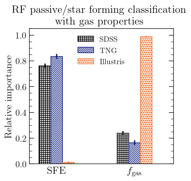
Figure 16: Feature importance in the Random Forest classification into star forming and passive galaxies, using $f_{\rm gas}$ and SFE as input features. The algorithm is allowed to choose from all features at each split. SFE clearly dominates in the observations and holds over three times more predictive power than $f_{\rm gas}$. In Illustris quiescence is more accurately predicted by $f_{\rm gas}$, while in TNG SFE holds significantly more predictive power, in agreement with the SDSS observations.

5.1.2 RF classification with $f_{\rm gas}$ and SFE

As a final consideration in this discussion, we perform a random forest classification on Illustris, TNG and the SDSS, using $f_{\rm gas}$ and SFE as input features for the algorithm. In Fig. 16 we show median feature importances extracted from 500 realisations of a forest for each data set, marking the 5th and 95th percentiles of the importance distribution with the vertical error bars.

It is apparent in Fig. 16 that SFE holds more predictive power than $f_{\rm gas}$ in the SDSS, where its relative importance is over twice that of gas fraction (in agreement with Ellison et al. (2020)). As expected from our previous analysis in Sec. 4.4, the TNG result makes a prediction similar to the observed trends, where the cumulative information gain provided by the SFE in the classification is higher than that of $f_{\rm gas}$ by over 3 times. In Illustris the predictions also summarise our previous analysis very well. The suite predicts $f_{\rm gas}$ to hold almost all predictive power in determining whether a given galaxy is star-forming or quenched. This result further illustrates how the AGN feedback in Illustris primarily acts to deplete molecular gas reservoirs to prevent future star formation, without substantial changes in star formation efficiency.

Our consistent comparison between observations and theoretical predictions from the simulations suggests that AGN can potentially affect their galaxies through a combination of thermal energy and momentum injection into the surrounding gas. In this scenario, the central black hole will both maintain high temperatures in the halo gas, not allowing reservoir replenishment; and increase turbulence in the ISM, resisting gravitational collapse. Our RF experiment with molecular gas properties shows that TNG agrees with the observations, while Illustris does not. This result points towards a success of the kinetic mode over the mechanical bubble implementation in the AGN feedback model development within the Illustris framework.

Following the encouraging qualitative agreement between the SDSS and the simulations, we would expect massive enough black holes to cause and maintain low star formation rates in their galactic hosts. The AGN could achieve that through a radiatively inefficient feedback channel, injecting turbulence into the ISM as well as increasing the temperature and entropy of the CGM. Such an AGN feedback model would result in both a decrease in gas fractions and star formation efficiency, preventing gravitational collapse and subsequent star formation. In this paradigm, the AGN feedback could be observed in action through direct measurements of molecular gas content and kinematics across the galaxy coupled with a direct measurement of black hole mass. Unfortunately, these three kinds of observations are not simultaneously available for large galaxy samples at the moment and hence the detailed tests of this theoretical prediction can only be completed in the future.

5.1.3 $L_{\rm AGN}$ and ${M_{\rm BH}}$ – consequences for direct AGN feedback observations

Our analysis in Sec. 4.3.1 carries important implications for the observational interpretation of AGN quenching. Since black hole accretion rate is responsible for the measured bolometric luminosity of an AGN, the negligible importance of instantaneous ${\dot{M}_{\rm BH}}$ implies little significance of AGN detection and classification for the study of black hole quenching in action. In fact, this prediction explains why a substantial body of research in the field delivers contradicting results, with some authors finding a relationship between the current AGN activity and quenching (e.g. Nandra et al., 2007; Bundy et al., 2008; Georgakakis et al., 2008), while others find no evidence of such a relationship (e.g. Rosario et al., 2013; Aird et al., 2012) for different samples of AGN hosts.

The negligible importance of ${\dot{M}_{\rm BH}}$ in the simulations, however, does not imply that black holes are not responsible for quenching of star-formation in massive central galaxies. As we explain in Section 4.3, it is the fossil record of the integrated AGN activity, traced by ${M_{\rm BH}}$, rather than its instantaneous power injection at $z=0$ traced by ${\dot{M}_{\rm BH}}$, which can successfully predict which galaxies are no longer star forming. This statement is true for all three different prescriptions for AGN feedback implemented in EAGLE, Illustris and TNG and does not make any assumptions about the functional form of $\dot{M}_{\rm BH}(t)$.

The redshift $z=0$ measurement of $M_{\rm BH}=\int\dot{M}_{\rm BH}\,{\rm dt}$ in the simulations is agnostic to whether e.g. a single violent event was responsible for the bulk of the growth of ${M_{\rm BH}}$ or whether it was a slow growth through constant low-${\dot{M}_{\rm BH}}$ over time. Hence, it would be interesting to investigate the importance of peak black hole accretion rates for the star-forming/quenched classification to compare them against ${M_{\rm BH}}$ measurements. Unfortunately, owing to the nature of black holes and the ‘no-hair theorem’ (Misner et al., 1973) it is impossible to infer their exact accretion history from contemporaneous observations. Being limited to simulations only, we would not be able to make a comparison between theoretical predictions and the observable Universe, which is the key objective of this work.

As we show in Sec. 4.3.1, all three simulation suites predict different distributions in $L_{\rm AGN}$ between the star forming and passive galaxy populations, stemming from their different prescriptions for AGN feedback. The model favoured most in comparison with observations – TNG – predicts higher AGN luminosities in star forming galaxies. This observational signature is expected in a cold mode accretion scenario where there is abundant dense gas available to feed both the black hole accretion disk in the galactic centre as well as the star formation within the galactic disk. Once the accretion becomes inefficient and the feedback mode changes, black holes are still accreting hot gas, which is sufficient to provide AGN feedback of the mechanical kind.

As we show in our analysis, this mechanism most strongly affects the efficiency of star formation, hence causing the association of quenched galaxies with primarily low accretion rates (and hence AGN luminosities). These results suggest that the most violent processes observed in the AGN during their quasar phase are associated with episodes of thriving star formation rather than galactic quiescence, and it is the inefficient accretion of hot gas onto the black hole environment which ultimately maintains galaxies in their very low star formation state. In fact, such trends have already been reported in the observational literature by e.g. Hickox et al. (2009), Xue et al. (2010), Heckman & Best (2014) and Trump et al. (2015).

Even if we refrain from identifying the model most compatible with the observable Universe, there are further reasons for which a measurement of $L_{\rm AGN}$ in large studies of currently active AGN is non-trivial to interpret in the context of quenching. All three simulations analysed in this study invoke supermassive black hole feedback in order to successfully quench their massive galaxies, however they implement different subgrid treatments to achieve this goal. As we see in our analysis all three prescriptions predict three different AGN luminosity trends between the passive and star-forming galaxy populations. In contrast, EAGLE, Illustris and TNG unanimously predict an association between high black hole masses and quiescence, regardless of the model assumptions. Therefore ${M_{\rm BH}}$ proves to be a robust tracer of AGN feedback quenching, insensitive to its exact mode of operation, whereas the connection between $L_{\rm AGN}$ and quenching is highly model-dependent.

The robustness of black hole mass is not only restricted to predictions drawn from numerical simulations. Ultimately, a condition necessary for a quenching mechanism to succeed is being able to offset the cooling rates within the halo. Without enough heat continuously provided into the CGM, the halo gas would cool and accrete onto a galaxy, leading to an ever-active star formation as a consequence of a ‘cooling catastrophe’. As shown analytically in Appendix B by Bluck et al. (2020a), the energy required for an AGN to offset cooling in the halo is directly proportional to ${M_{\rm BH}}$, which is the integral of ${\dot{M}_{\rm BH}}$ over time. These considerations do not make any assumptions about the microphysics of AGN heating and, instead, universally show how the instantaneous behaviour of accretion has no immediate impact on the galactic evolution cycle. From this simple argument one would yet again expect to observe quenching signatures as a function of black hole mass rather than luminosity of active galactic nuclei, as is indeed confirmed in three leading hydrodynamical models here, with differing feedback prescriptions.

5.1.4 Lessons learned from observational realism

In the process of comparing data on equal footing, we had a unique chance to look at simulation results from the perspective of observational realism. As a result we find that cosmological simulations produce smaller passive populations than the observed Universe. This issue is particularly visible in Illustris, where quiescent central galaxies account for only $\sim 12\%\,(\sim 35\%)$ of the whole population with $M_{\ast}>10^{10}\,(M_{a}st>10^{10.6})$. The situation in EAGLE is less dramatic since the suite manages to produce a quiescent population of $\sim 25\%\,(\sim 42\%)$ among massive centrals in these mass ranges. Finally, TNG produces the largest passive population amounting to $\sim 34\%\,(\sim 67\%)$, however this fraction is still lower than the $\sim 50\%\ (\sim 68\%)$ we see in the SDSS (calculated with volume corrections to account for the Malmquist bias). We also learn that if the intrinsic behaviour of different galactic parameters as a function of ${M_{\rm BH}}$ is almost a step function, the current measurement uncertainties in the observations may very well hide it, producing very smooth curves like in the case of TNG.

Finally, the simulated galaxy trends seem to predict relations observed in the Universe rather well without accounting for the measurement uncertainty. One obvious example of this property is the simulated Main Sequence which is potentially too wide across all data sets. EAGLE, Illustris and TNG all reproduce the observed width of the MS very well, however when we account for more realistic observations by adding random scatter informed by the observations, the $M_{\ast}-{\rm SFR}$ relations become significantly too spread out. This result suggests that the intrinsic Main Sequence relation is quite tight and, more importantly, tighter than predicted by the simulations. This may in turn point towards MS regularisation processes that are overlooked in the currently available models.

We do, however, want to note that our realism treatment here is rather simplistic - we do not perform full radiative transfer calculations to obtain simulated galaxy spectra and hence we do not use the same techniques to estimate relevant galactic parameters in both simulations and observations. Nonetheless, regardless of their simplicity our realism steps do account for the three main caveats associated with the SDSS observations - fibre aperture correction, S/N ratio cuts on emission line fluxes and the random measurement errors.

6 Summary and conclusions

In this work we investigate the physical mechanisms responsible for quenching in massive central galaxies by analysing multiple sets of theoretical predictions and testing them against observations of the local Universe. More specifically, we make use of the publicly available data from three state-of-the-art cosmological simulations: EAGLE (Schaye et al., 2015; Crain et al., 2015), Illustris (Genel et al., 2014; Vogelsberger et al., 2014b, a; Sijacki et al., 2015) and TNG(Marinacci et al., 2018; Naiman et al., 2018; Nelson et al., 2018; Springel et al., 2018; Pillepich et al., 2018b), to understand how star formation is quenched in these approximations of our Universe. We then compare the detailed predictions from these three simulations to observational measurements from the SDSS. Because all three simulations invoke AGN feedback as their primary tool to shut down star formation in massive centrals, we have a perfect opportunity to thoroughly explore this quenching avenue in the local Universe.

We first perform a Random Forest experiment to determine which parameter among ${M_{\rm BH}}$, ${M_{\ast}}$, ${M_{\rm halo}}$ and ${\dot{M}_{\rm BH}}$ (in the case of simulations) holds the most predictive power in determining whether a given galaxy is star forming or quenched. We then follow up the outcome of machine learning with a partial correlation analysis, to investigate the relationships between different variables and check whether their connection with quiescence is intrinsic or incidental. As a final step we analyse the behaviour of gas content of galaxies during their transition towards quiescence. In order to do this we infer ${\rm H_{2}}$ masses from optical extinction in the SDSS spectra and compare the observations to the published HI/${\rm H_{2}}$ catalogues in Illustris and TNG. Our primary results are as follows:

1. the Random Forest analysis reveals black hole mass as the most important parameter for classifying a galaxy into a quenched or star forming category. This result is a unanimous prediction of all three simulations and thus independent of the exact implementation of the AGN feedback model. It is also true in the SDSS, where it is invariant under different choices of ${M_{\rm BH}}$ calibration used in lieu of dynamical measurements of black hole mass. Our comparison between simulations and observations puts forward the dominance of black hole mass as the most robust observable consequence of AGN feedback quenching in massive central galaxies. This prediction is met exceptionally well in the SDSS which suggests that supermassive black hole feedback is the most likely quenching avenue in observed central galaxies (Figs.5 & 6).
   

2. when we calculate the partial correlation coefficients we find that other galactic parameters like ${M_{\ast}}$ and ${M_{\rm halo}}$ are both predicted and observed to carry little intrinsic correlation with a reduction in sSFR. Instead, their their connection to quenching found previously through a direct correlation analysis proves incidental once the ${M_{\rm BH}}$-${M_{\ast}}$ and ${M_{\rm BH}}$-${M_{\rm halo}}$ relationships are accounted for (Figs. 10 & 11).
   

3. simulations predict a negligible importance of ${\dot{M}_{\rm BH}}$ in comparison with ${M_{\rm BH}}$. This finding suggests that the observational search for AGN feedback quenching should focus on the integrated history of the AGN feedback (encoded in ${M_{\rm BH}}$) rather than the instantaneous activity of the AGN (as captured by $L_{\rm AGN}$) (Figs. 7 & 8)
   

4. moving on to the evolution in gas content and quiescence, we find that quenching is associated with both a reduction in SFE and $f_{\rm gas}$, estimated within the SDSS fibre in the observations (Figs. 12 & 13). We also find that it is SFE rather than $f_{\rm gas}$ which holds the most predictive power in determining the star-forming / passive classification when only these two parameters are considered by the RF algorithm (Fig. 16).
   

5. when we compare theoretical predictions with the SDSS, we find that TNG predicts trends more consistent with observations than Illustris. We find the most visible disagreement in SFE, which rises with increasing black hole mass in Illustris and decreases in TNG (as it does in the SDSS). Once we add observational realism to the data, these differences are highlighted even more: quiescent galaxies in Illustris form stars efficiently at their centres, while their TNG counterparts remain quiescent at their cores. At the same time we stress that although TNG shows good qualitative predictions for the observed trends, observations do not match them in the highest ${M_{\rm BH}}$ bins, where gas fractions and in-fibre sSFRs are significantly lower in TNG than in the SDSS (Figs.14 & 15). More importantly, however, TNG also significantly overestimates the quenching thresholds in ${M_{\rm halo}}$ and ${M_{\rm BH}}$ when compared with the SDSS (Fig. 3).

Our Random Forest experiment, together with the partial correlation analysis show results consistent with an AGN quenching scenario and inconsistent with other quenching mechanism like e.g. supernova feedback or virial shock heating. All three simulations predict a negligible association between ${\dot{M}_{\rm BH}}$ (and, by extension $L_{\rm AGN}$) and quiescence, regardless of their subgrid treatment of AGN feedback. This finding might explain why previous studies aimed at linking elevated AGN activity with quenching delivered ambiguous results in which different authors were finding both positive and negative correlations between $L_{\rm AGN}$ and quiescence or even a lack thereof. The difference in timescales between the change in SFR and the change in ${\dot{M}_{\rm BH}}$ (the AGN duty cycle) is crucial for the potential appearance of these correlations in the observable Universe, as argued by e.g. Hickox et al. (2009) and Harrison et al. (2019). Hence, in this study a clear picture emerges in which it is the the total power output of the AGN integrated over time, i.e energy, which dictates the fate of a galaxy rather than its instantaneous activity. The simulations clearly show how different prescriptions for AGN feedback implementation result in contradictory trends in the $L_{\rm AGN}$ observable, while the picture in ${M_{\rm BH}}$ is consistent across the suites. We therefore conclude that black hole mass is a more robust tracer of AGN feedback than ${\dot{M}_{\rm BH}}$, boasting independence of the model prescription for the feedback mode of operation.

Finally, through our analysis of molecular gas content we find the most probable mode of operation of the AGN. We show how the central black hole has influence on both a) depleting the star forming gas reservoirs and b) decreasing the efficiency with which the remaining gas is collapsing to form new stars. We learn that a successful AGN feedback model most likely involves a combination of turbulence injection and heating, which leads to the observed depletion of molecular gas and decreased star formation efficiency upon transition to quiescence.

Data availability

All data used in this study have been previously published and are available at the following online locations:

• EAGLE: virgodb.dur.ac.uk/

• Illustris: www.illustris-project.org/

• TNG: https://www.tng-project.org/

• MPA-JHU release of spectrum measurements:
  wwwmpa.mpa-garching.mpg.de/SDSS/DR7/

• SDSS Group Catalogue: gax.sjtu.edu.cn/data/Group.html

• NYU Galaxy Value Added Catalogue:
  sdss.physics.nyu.edu/vagc/

• morphological catalogues:
  doi.org/10.1088/0067-0049/196/1/11
  doi.org//10.26093/cds/vizier.22100003

Appendix A sSFR function

Due to the lack of ${\rm H\alpha}$ detections in the passive sequence in the SDSS, one is not able to measure accurate SFRs to arbitrarily low specific star formation rate values. This problem is dealt with in Brinchmann et al. (2004) by imposing an upper limit of log(sSFR/${\rm yr^{-1}}$) $\sim-12$ for quiescent systems, as indicated by the lack of emission lines and a large magnitude of the D4000 break.

In the simulations there is no limit on sSFR, since it is possible for a given galaxy to have SFR=0 if none of its gas cells/particles reach density and temperature thresholds required for star formation. As shown in the left panel in Fig. 17 the distribution of sSFR extracted directly from the simulations coincides with the SDSS quite well at high sSFR values, however it extends far beyond the observational limit on the low-sSFR end. Because simulations can, in principle, have $\log({\rm sSFR})$ distributions extending down to $-\infty$, showing a comparison between them and the observations proves difficult in logarithmic units.

Hence, in order for us to include all simulated galaxies in Figs. 2, 12 and 13, we redistribute all objects with log(sSFR/${\rm yr^{-1}}$) $<-12$ to values drawn from a distribution of $\log({\rm sSFR})$ in the passive population in the SDSS. More precisely, we treat the sSFR density function for all galaxies with log(sSFR/${\rm yr^{-1}}$) $<-11$ in the SDSS as a probability distribution and for each qualifying galaxy we draw a new ‘redistributed’ sSFR value at random. As we show in the right panel of Fig. 17, the amended sSFR density function in all simulations matches the observed distribution quite well at the low-sSFR end. Most importantly, there are no more low-sSFR objects extending below the imposed sSFR limit in the SDSS, allowing us to show the whole simulated quenched population in the $M_{\ast}-{\rm SFR}$ plane.

Finally, we would like to stress that this redistribution is performed for visualisation purposes only and the newly assigned sSFR values do not enter any of our quantitative analysis presented in Sec. 4.1-4.5.

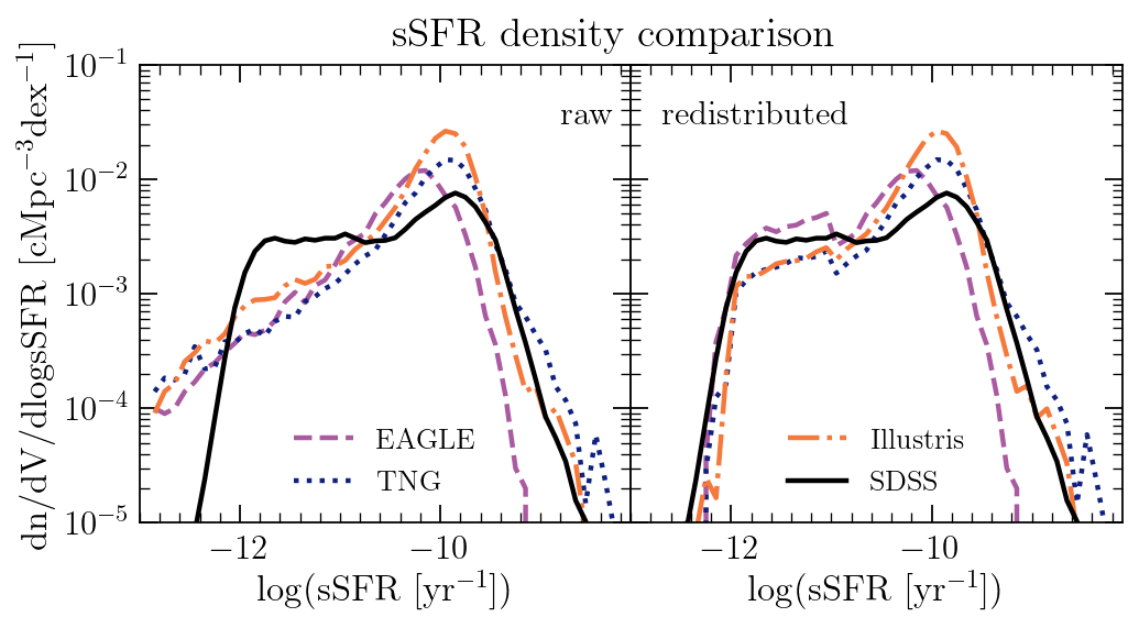
Figure 17: Comparison of the sSFR comoving density in simulations and observations: left: as simulated, right: with simulation results redistributed to reflect the technical limitations associated with measuring low sSFRs in the observable Universe. The RHS result was constructed by redistributing each object in the simulations with log(sSFR/${\rm yr^{-1}}$) $<-12$, randomly drawing from the SDSS distribution for objects with log(sSFR/${\rm yr^{-1}}$) $<-11$. The SDSS distribution was weighted by $1/V_{\rm max}$ to correct for the Malmquist bias.

Appendix B Robustness of the Random Forest classifier results

One of the key parts of our analysis relies on Random Forest classification to determine which of the galactic parameters is most predictive for deciding whether a given galaxy has ceased its star formation by redshift $z=0$. Although the use of machine learning techniques is gradually becoming more common in astronomy, we appreciate how the choice of our tool can raise potential questions about the result interpretation, as well as its reproducibility. In order to better understand the RF result and how the characteristics of the data influence the inferred feature importances, we present a range of tests of this method in this section.

B.1 Restricting the number of features available in each split

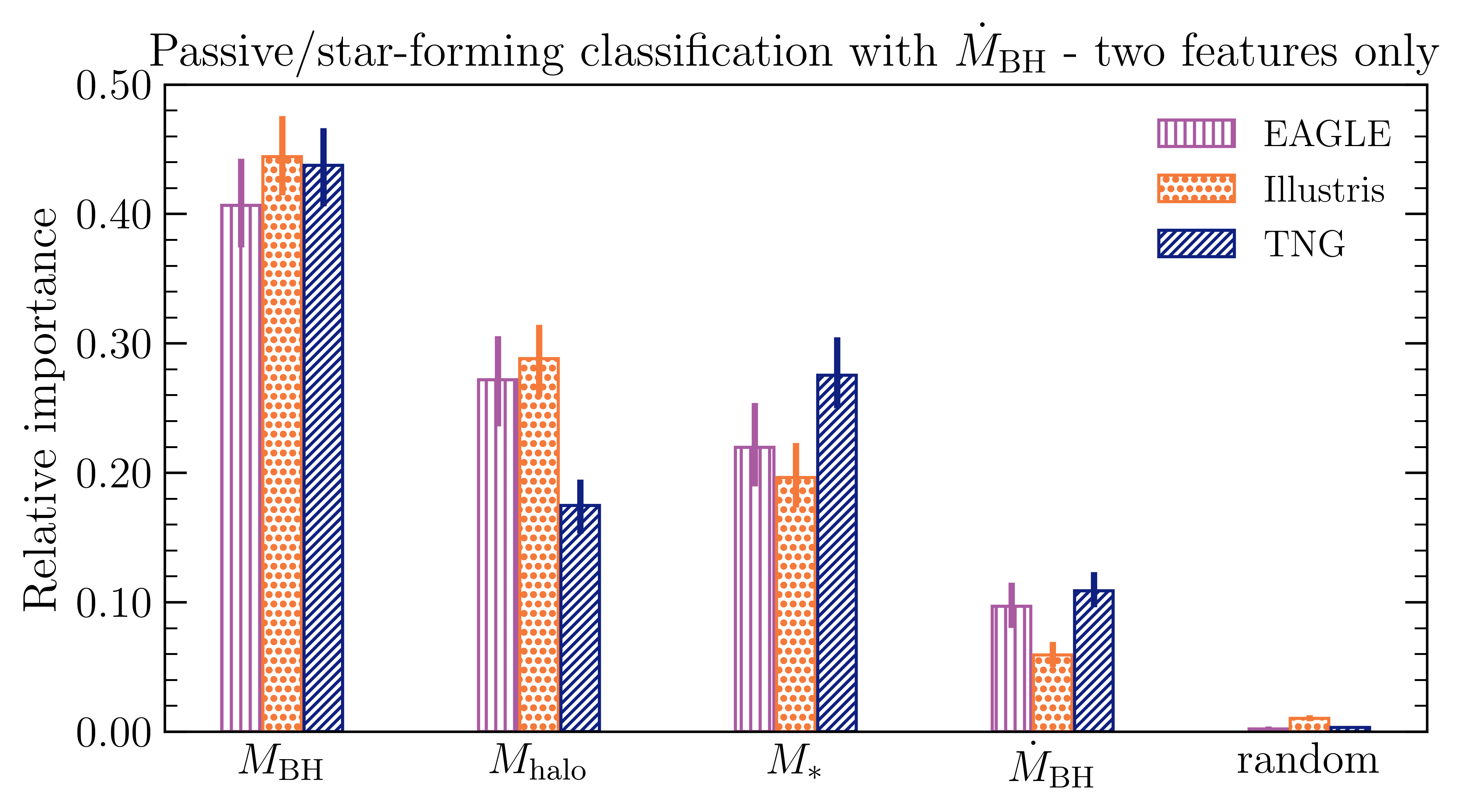
Figure 18: Same as left panel in Fig. 19 with ${\dot{M}_{\rm BH}}$ parameter added to the list of features. Among all other investigated parameters ${\dot{M}_{\rm BH}}$ carries least predictive power in determining galaxy classification.

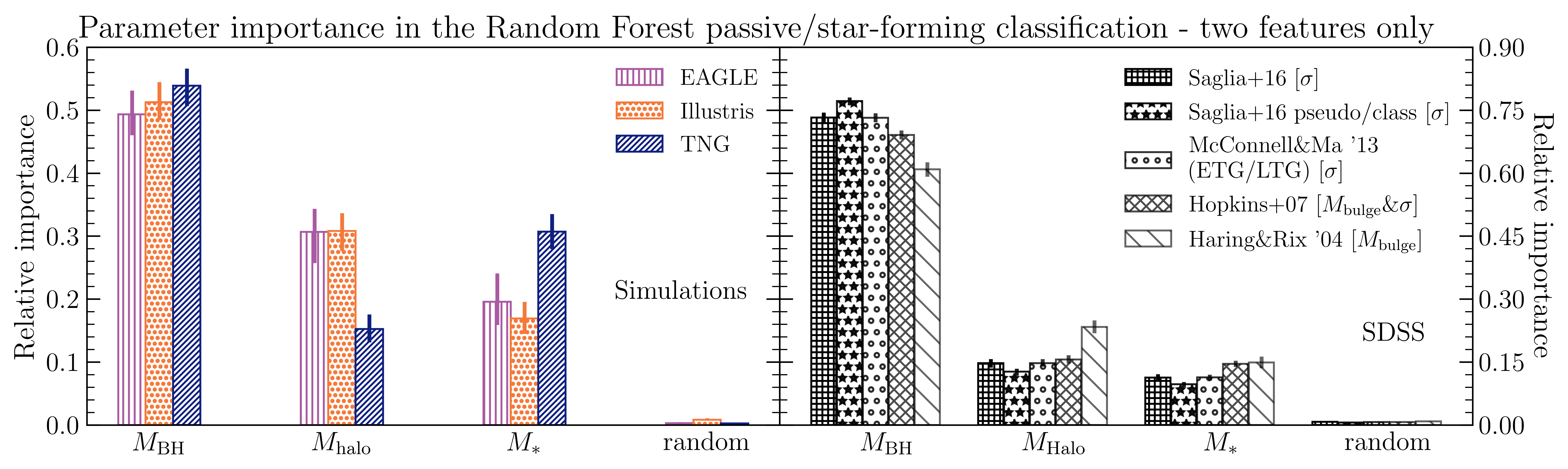
Figure 19: Same as Fig. 5 with features restricted to a random draw of two features at each split. Error bars indicate the 16th and 84th percentiles of the distribution in parameter importance drawn from 500 realisations of the experiment. Left panel: in simulations ${M_{\ast}}$ and ${M_{\rm halo}}$ pick up importance owing to their inter-correlation with ${M_{\rm BH}}$. Right panel: in SDSS the rise in importance of other parameters is less pronounced than in the case of simulations.

As we mention earlier in Sec. 3.3, one means of additional randomisation in an RF architecture is forcing the algorithm to randomly sample features available for a given split. Empirical tests with different RF architectures suggest that restricting the number of available features improves algorithm performance on previously unseen data in the presence of noise associated with its measurement (Breiman, 2001). This increase in robustness comes at a cost of a decreased ability of the algorithm to remove inter-correlation within the data. Because our work does not focus on predicting unknown sSFR classes and, instead, aims to extract causality in our simulated and observed data sets, we allow our algorithm to choose from all features at every split by default. In order to check whether restricting the number of available features can influence our main conclusions, we conduct our experiment again, randomly choosing 2 features at each node. We check that our conclusions are robust against this choice in the algorithm architecture.

In Figs. 18 & 19 we explore the change in feature importances when the decision trees randomly select a subset of two features to split on at every node. The visible dominance of ${M_{\rm BH}}$ over other parameters is well preserved in both the simulations and the observations, however this time other parameters gain on importance in comparison with the RF architecture allowed to choose from all features at every split in Figs. 5 & 6. When comparing the left panel in Fig. 18 and Fig. 19 alone, we see once again that the ${\dot{M}_{\rm BH}}$ bar height is picked up primarily at the expense of the ${M_{\rm BH}}$ score, most likely owing to the connection between the two variables in the subgrid black hole accretion model.

The difference between all features and their random subsampling is more pronounced in the simulations, where black hole mass’ relative importance is only about twice the value of the next best ranked parameter. The difference between the SDSS and simulations is primarily dictated by how tight the relationships between ${M_{\rm BH}}$ and other parameters are in the data sets. Given the result in Fig. 19, we can safely assume that whenever the algorithm has a choice between black hole mass and another parameter (which statistically happens for a half of all splits) it is always ${M_{\rm BH}}$ which results in the highest reduction in impurity. For the remaining half of splits the tree has to make a decision among ${M_{\rm halo}}$, ${M_{\ast}}$ and a random number, in which case the feature in the closest numerical association with ${M_{\rm BH}}$ takes the split.

As we show in Sec. 4.3 the ${M_{\rm BH}}$-${M_{\ast}}$ and ${M_{\rm BH}}$-${M_{\rm halo}}$ relations are significantly tighter in the simulations and hence a split on a secondary feature results in a higher reduction in impurity in the simulations than in the observations. However, regardless of the change in relative importance of ${M_{\rm halo}}$ and ${M_{\ast}}$  Fig. 19 demonstrates that black hole mass is unanimously predicted to hold the most predictive power in determining whether central galaxies are star-forming or quenched in the simulations. This theoretical prediction is then validated in the observations, regardless of the ${M_{\rm BH}}$ calibration or the algorithm architecture.

B.2 Feature importances in correlated variables

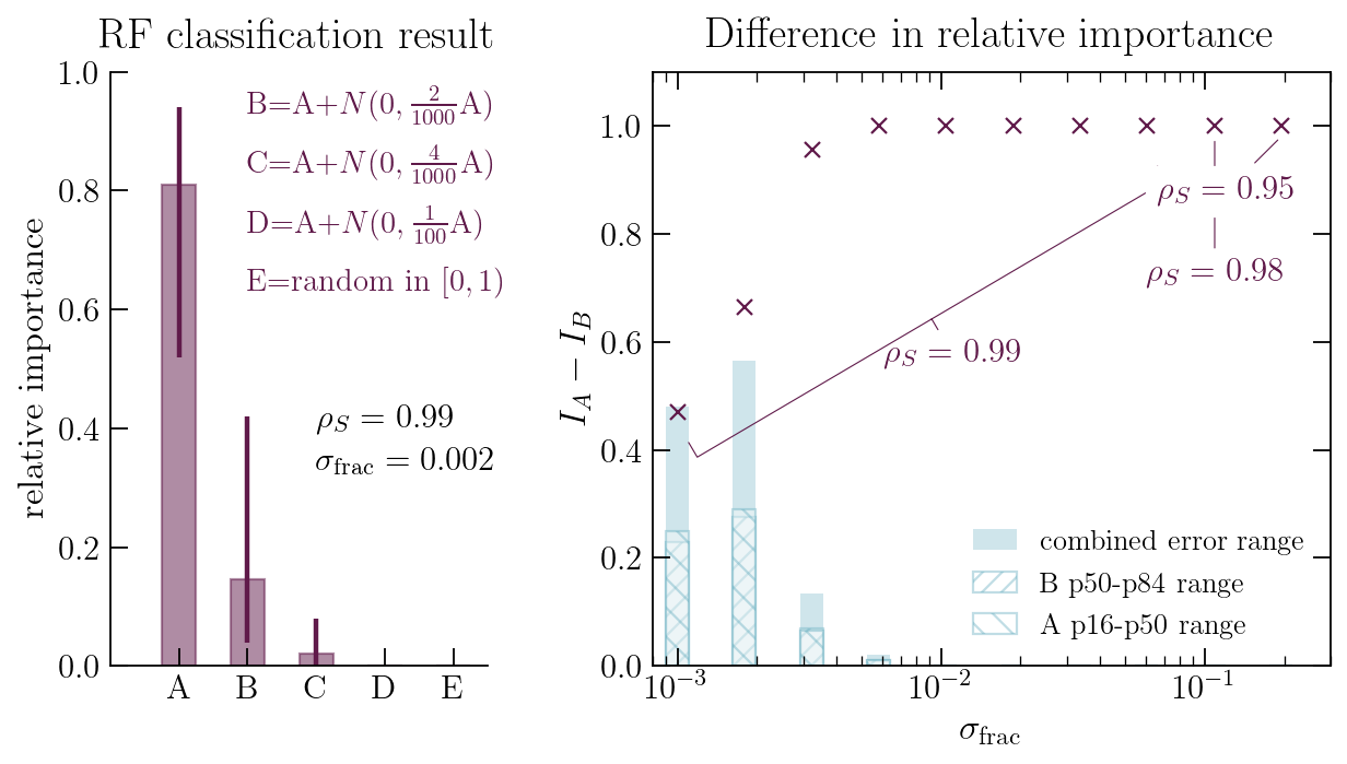
Figure 20: Left: feature importances of strongly correlated variables in an RF classification. Spearman’s rank correlation coefficient $\rho_{S}$ between A and B is 0.99 and the result corresponds to the 5th data point from the left in the right plot. Variable A assigns the class labels and hence performs best, followed by B, C, D in the order of increasing noise. Right: same RF experiment repeated for different levels of noise in B, showing the difference in feature importance (A-B) along with associated error ranges. Crosses in blue shaded regions show where the result is inconclusive. The figure demonstrates how successful the RF algorithm is at picking the most relevant parameter at $\sim 1\sigma$ confidence at $\rho_{S}=0.99$ between the two most successful variables.

As we explore in detail in Sec 4.3, all variables of interest in both simulations and the SDSS are relatively strongly inter-correlated with one another. This close connection among galactic parameters can raise concerns as to whether the Random Forest is able to identify the true feature carrying the most importance in the classification, with an appropriate degree of confidence.

We illustrate this potential issue in the EAGLE suite as an example, where ${M_{\rm BH}}$ and ${M_{\rm halo}}$ are the two variables scoring highest out of all parameters in Fig. 18. When we plot ${M_{\rm BH}}$ against ${M_{\rm halo}}$ in Fig. 11, we see a strong correlation between the two. Without the PCC analysis we cannot a priori assume which of the parameters is intrinsically connected to quenching and which of them earns feature importance owing to the correlation strengths with other parameters. Hence, the question is how strongly would ${M_{\rm halo}}$ and ${M_{\rm BH}}$ have to be correlated, in order for the black hole mass dominance to be an ambiguous result in the Random Forest classification.

To check when the above is true, we design a test of the RF framework, using synthetic variables which are related to one another via straightforward functional forms. In our synthetic data set we create 10 000 objects to mimic the sample sizes in this work, each with an entry for variables A, B, C, D and E. We first choose the variable A, which is a set of real numbers $y=x^{2}$, where $x$ is drawn at random from a flat distribution in $[0.5,1.5)$. The exact choice of the functional form of $y(x)$ does not affect the results of this test. The range of values in A is chosen such that we can think of it as a measurement of SFR in the real data.

We then create B, C and D by adding random draws from a Gaussian centred on 0 to A such that ${\rm B=A}+N(0,\sigma_{\rm B}\times{\rm A})$, ${\rm C=A}+N(0,\sigma_{\rm C}\times{\rm A})$ and ${\rm D=A}+N(0,\sigma_{\rm D}\times{\rm A})$. The amount of scatter we add to a given measurement in A changes with A such that the scatter around $\log({\rm A})=\log({\rm B})$ is constant across the whole range in A. We choose $\sigma$ values to increase from B to D such that these parameters are respectively most and least closely correlated with A. In particular, we choose $\sigma_{\rm C}=2\sigma_{\rm B}$ and $\sigma_{\rm D}=5\sigma_{\rm B}$ to ensure significant differences among the parameters. Finally, like in the case of our fiducial RF analysis, we also include a random draw from a flat distribution in $[0,1)$ which becomes the E variable.

Once a given set of synthetic parameters is created, we assign a class label for each object based on A, such that all objects with ${\rm A}\leq 1.5$ are labelled as ‘passive’ and the rest are ‘star forming’. We then repeat the Random Forest classification 500 times, calculate the resulting median feature importances and estimate their uncertainties from the 16th and 84th percentiles of each distribution. The full test consists of 10 different realisations of the synthetic data in which we increase $\sigma_{\rm B}$ from 0.001 to 0.2 in equally spaced logarithmic steps, decreasing the strength of correlation between variables A and B in each step. Finally, in order to quantify their numerical association we calculate their Spearman’s rank correlation coefficient $\rho_{S}$ in each realisation.

Table 7: Sperman’s rank correlation coefficient $\rho_{S}$ calculated between black hole mass and other RF parameters for all data sets. In SDSS $\rho_{S}$ is calculated separately for each ${M_{\rm BH}}$ estimator and takes into account the $\ifrac{1}{V_{\rm max}}$ and inclination corrections.

	${M_{\rm BH}}$–${M_{\rm halo}}$	${M_{\rm BH}}$–${M_{\ast}}$	${M_{\rm BH}}$–${\dot{M}_{\rm BH}}$
EAGLE	0.85	0.82	0.62
Illustris	0.84	0.87	0.49
TNG	0.90	0.95	0.19
Saglia+16 $[\sigma]$	0.80	0.82	–
Saglia+16	0.79	0.81	–
pseudo/class $[\sigma]$
McConell&Ma ’13	0.79	0.81	–
(ETG/LTG) $[\sigma]$
Hopkins+07	0.87	0.89	–
$[M_{\rm bulge}\&\sigma]$
Haring&Rix ’04	0.91	0.92	–
$[M_{\rm bulge}]$

Fig. 20 presents the result of our Random Forest test, showing how strongly two test variables A and B need to be correlated in order for the classifier to produce an ambiguous ranking of feature importances. We show a representative RF classification result for $\sigma_{\rm B}=0.002$ in the left panel, where bar heights indicate feature importances, while the error bars encapsulate the 16th and 84th percentiles of feature importance distributions. The functional form connecting the variables is also listed in the left panel. In the right panel we show how the difference between median importances in A and B ($I_{A}-I_{B}$, bordeaux crosses) changes as a function of $\sigma_{\rm B}$ ($\sigma_{\rm fractional}$ in the figure). The hatched bars indicate the magnitude of the negative uncertainty on A and positive uncertainty on B, while the blue shaded bars show the total of the two. Whenever a cross is within the blue bar, the feature importance of A and B agree within their errors. Additionally, the panel lists the measurement of $\rho_{S}$ between the two variables for each of the 10 realisations of synthetic data.

The first thing to notice in Fig 20 is that the value of $I_{A}-I_{B}$ is always positive, hence the most important parameter in the classification is always identified, regardless of how closely the next best variable is associated with it. The significance of this result, however, differs as indicated by the location of bordeaux crosses with respect to the blue shaded bars. Most importantly, we can see how the significance of $I_{A}-I_{B}$ varies as a function of $\rho_{S}$. It is clear that even for the extreme case of $\rho_{S}=0.99$ the most relevant parameter is selected by the RF algorithm at a confidence level of $\sim 1\sigma$.

The Random Forest robustness test in Fig. 20 demonstrates how incredibly successful the method is at selecting the most important parameter among strongly inter-correlated variables. In order to see how this test supports our RF results in Sec 4.2 and Appendix B.1, we calculate $\rho_{S}$ between ${M_{\rm BH}}$ and each of ${M_{\rm halo}}$, ${M_{\ast}}$ and ${\dot{M}_{\rm BH}}$ in turn, summarising the values in Table 7. It is apparent that galactic parameters in both the observed and simulated data in our analysis never reach the threshold required for the Random Forest result to be ambiguous. The highest correlation coefficient we measure is between ${M_{\rm BH}}$ and ${M_{\ast}}$ in TNG, reaching $\rho=0.95$ – a correlation strength at which the most important parameter is identified with full confidence. Therefore we conclude that the unanimous victory of black hole mass over other galactic parameters in the Random Forest experiment is a robust result, unaffected by the strong inter-correlations present among the variables in the investigated data.

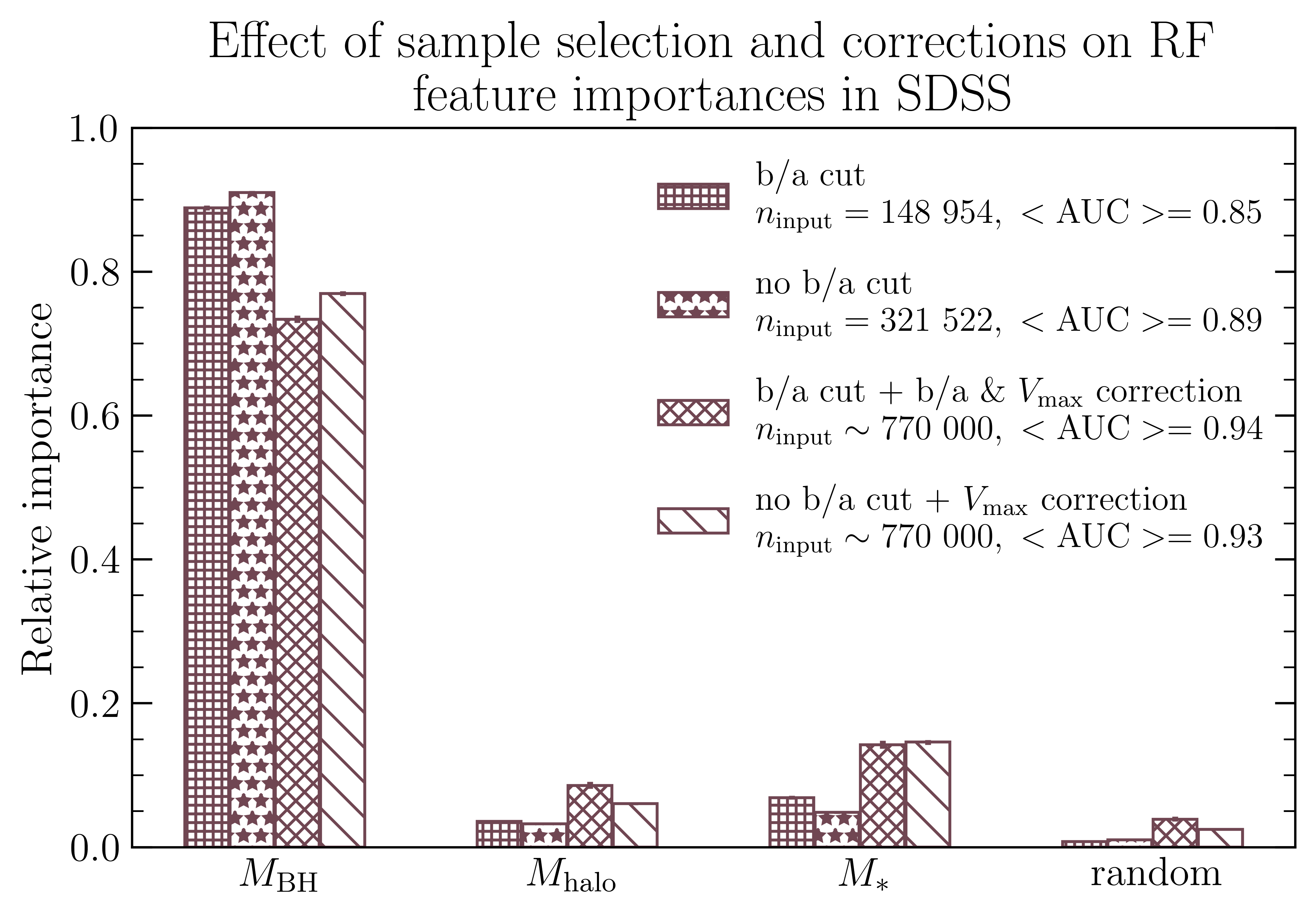
Figure 21: Testing the effect of adding corrections and/or removing an inclination cut on RF feature importances in the SDSS. It is apparent that ${M_{\rm BH}}$ remains clearly the most important parameter, regardless of the tested input data set.

B.3 Including sample corrections in the RF

Another issue to consider when approaching our classification result for the SDSS galaxies, is accounting for the volume weighting and inclination correction within the Random Forest experiment. We can achieve such corrections by drawing a large sample of objects with replacement from the following probability distribution:

$$p_{i}=\frac{\omega_{i}}{\sum_{i}\omega_{i}},$$ (23)

where $\omega_{i}$ is the combined weight defined earlier in Eq. 19. In this way objects with higher weights (predominantly low-mass and star-forming galaxies) are more likely to be drawn and hence enter the input sample several times. The astronomical instinct to correct for the unobservable parts of the Universe, however, is in conflict with the machine learning algorithm, which assumes that the training and testing sets are disjoint and hence the testing exclusively involves previously unseen data. Upon random splitting into the test and training sets the same repeated object will undoubtedly be found in both of them, violating this assumption. In order to convince ourselves, however, that ignoring individual object weights does not affect our main conclusions, we implement the RF algorithm in four different scenarios, testing how adding corrections and/or removing the inclination cut on disks affects the resulting feature importances.

Fig. 21 shows the effect of adding corrections and/or removing an inclination cut on RF feature importances in the SDSS. It demonstrates that ${M_{\rm BH}}$ is by far the most important parameter among all three, regardless of the applied sample cuts and corrections in the Random Forest algorithm. Hence we conclude that our conclusions in Sec. 4.2 for the SDSS which do not include the $1/V_{\rm max}$ and inclination corrections are both: a) consistent with the ones reached with these corrections implemented; and, b) what is crucial, consistent with the main assumptions of the Random Forest algorithm.

Finally, we also learn that introducing corrections inflates the AUC score, as expected from the repeated exposure to the same objects in both the training and testing samples. This repetition is also responsible for the increased importance of a random number in classification. Removing the inclination cut with no correction effectively adds uncertainty to the ${M_{\rm BH}}$ values, since the $\sigma_{\ast}$ measurement in highly inclined disks becomes a noisy tracer of disk rotation. This is apparent in the decreased importance of ${M_{\rm BH}}$ in comparison with other parameters. One can also notice that accounting for the Malmquist bias and the inclination correction swaps the order of ${M_{\rm halo}}$ and ${M_{\ast}}$, potentially owing to a higher precision with which the latter is measured.

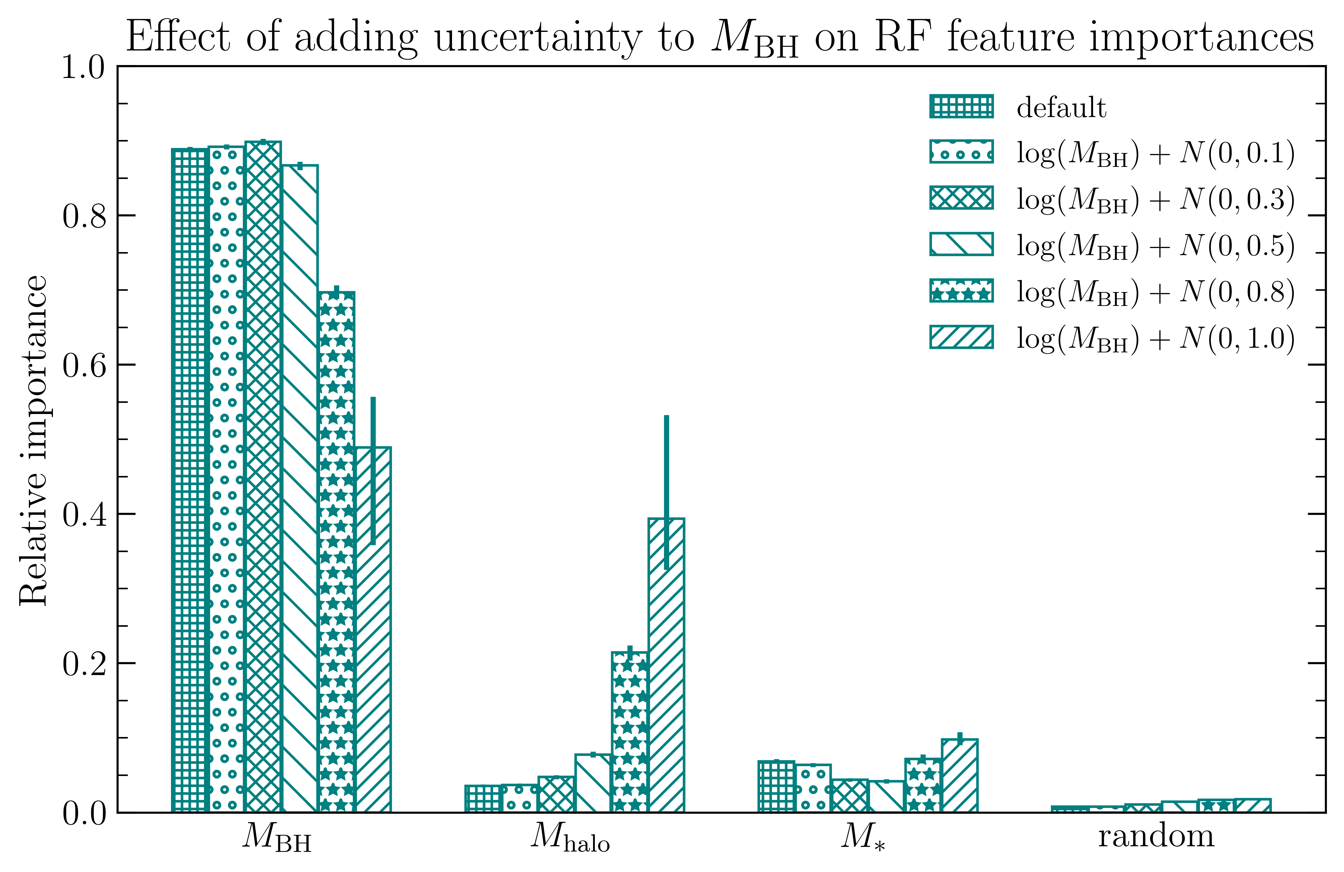
Figure 22: The effect of adding scatter to ${M_{\rm BH}}$ estimates in the SDSS on RF feature importances. This test addresses the concern of the RF result being impacted by a hypothetical better precision in the $\sigma_{\ast}$ measurement as compared to ${M_{\rm halo}}$ and ${M_{\ast}}$. The figure shows that adding even as much as 0.8 dex of Gaussian random noise to ${M_{\rm BH}}$ does not allow other parameters to take the lead. This behaviour breaks down at around $\sim$1 dex added uncertainty, when ${M_{\rm halo}}$ and ${M_{\rm BH}}$ carry the same importance within $1\sigma$ uncertainty. This is significantly more than the estimated difference in precision with which we measure both parameters, equal to $\sim$0.1 dex (i.e. an order of magnitude less than required).

B.4 The influence of measurement uncertainty on feature importances

The last item in our Random Forest robustness discussion is the potential effect that parameter uncertainty can have on the order of feature importances output by the algorithm. This issue, of course, is only relevant for the SDSS, where each variable is associated with either a measurement error or an uncertainty introduced by the use of a calibration. Given that all parameters of interest are estimated with a range of unique methods, it is naturally expected for all parameters to be measured or inferred with different degrees of precision. The immediate worry in this scenario is for the algorithm to select the feature measured with the smallest error as the most informative one in the classification.

The reason for this is the fact that parameters with increased levels of noise (poorer measurement quality) are more likely to bury their connection to the class labels in their increased scatter. Similarly, more precise measurements are less likely to result in a misclassification because the observed and true values are closer together. Hence, in the hypothetical case of two parameters being equally predictive of quenching, the one with smaller measurement uncertainty would be identified as a stronger predictor in the pair.

In the context of our Random Forest experiment, we want to check whether the strong dominance of ${M_{\rm BH}}$ over ${M_{\rm halo}}$ and ${M_{\ast}}$ in the SDSS could be driven by the differences in precision with which all three parameters are measured. According to the published uncertainty estimates in our sample, stellar mass is the most precisely measured variable, with a median error of $\sim 0.15\ {\rm dex}$ on ${M_{\ast}}$. For black hole masses, the main source of uncertainty comes from the scatter about the $M_{\rm BH}-\sigma_{\ast}$ relation, which amounts to $\sim 0.45\ {\rm dex}$, around 3 times more than in the case of ${M_{\ast}}$. Finally, the halo masses are the least precise estimates in the SDSS and their standard error is assumed to be $\sim 0.5\ {\rm dex}$.

Given that the importance of stellar mass for the passive galaxy classification is lower than that of black hole mass, it is certain that ${M_{\rm BH}}$ is the more relevant parameter between the two. Increasing the quality of ${M_{\rm BH}}$ estimates in the SDSS would only lead to a bigger gap between these two feature importances, further highlighting the black hole dominance. In the case of halo mass the situation is different. If ${M_{\rm halo}}$ and ${M_{\rm BH}}$ are hypothetically equally predictive of quenching classification, then a slightly worse precision in ${M_{\rm halo}}$ measurement would cause its feature importance to be less than that of ${M_{\rm BH}}$.

In order to check whether the order of feature importances in the SDSS could be driven by the difference in measurement quality, we repeat the RF experiment for different levels of scatter added to ${M_{\rm BH}}$. In each trial we create an augmented dataset by adding random Gaussian noise centred on 0 to the ${M_{\rm BH}}$ measurement, such that $\log(M_{\rm BH,\ new})=\log(M_{\rm BH})+N(0,\sigma)$. Throughout this test we increase the value of $\sigma$ until the relative importance of ${M_{\rm BH}}$ and ${M_{\rm halo}}$ are comparable, to estimate how much more precisely black hole mass would have to be measured in order to drive our main conclusion. What we check for in this test is not how the individual uncertainty affects the order between ${M_{\rm BH}}$ and ${M_{\rm halo}}$ but rather what is the impact of a ‘differential measurement error’, i.e. the difference in precision between the two parameters.

In Fig. 22 we present the result of our test, which clearly shows how the difference between ${M_{\rm BH}}$ and ${M_{\rm halo}}$ decreases with increasing level of differential noise added to ${M_{\rm BH}}$ alone. It takes as much as an additional 1 dex scatter for the importance of ${M_{\rm halo}}$ to be comparable with ${M_{\rm BH}}$. This is a factor of 10 higher than the estimated difference in measurement quality between the two variables of $\sim 0.1$ dex. Therefore, we conclude that our Random Forest result is not driven by the differences in parameter uncertainty and that the overwhelming ${M_{\rm BH}}$ dominance is an intrinsic quality of AGN feedback quenching in massive central galaxies.

Appendix C Comparison with dynamical measurements of ${M_{\rm BH}}$

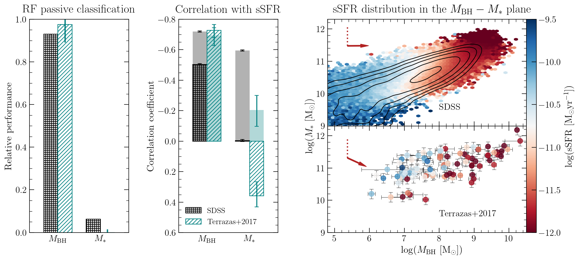
Figure 23: RF quenching classification analysis repeated with Terrazas+2017 data, compared to SDSS, showing that the conclusions we draw from our indirectly inferred ${M_{\rm BH}}$ are consisted with dynamically measured black hole masses. It is important to recognise, however, that the dynamically measured sample of black hole masses is not representative of the local Universe.

As a final consistency check of our method we investigate the reliability of calibrations to estimate ${M_{\rm BH}}$ in the SDSS galaxies. To this end we repeat our Random Forest and correlation analyses in a sample of 90 dynamically measured black hole masses in Terrazas et al. (2017). Because we only have access to two parameters: ${M_{\rm BH}}$ and ${M_{\ast}}$, we repeat the RF classification in the SDSS using these two parameters only, in order to compare both sets of observations side-by-side. We use the same algorithm architectures as before, requiring a minimum of 5 and 200 objects per leaf node in the Terrazas et al. (2017) sample and the SDSS respectively. In the SDSS we show the results using the calibration in Eq. 7 to estimate ${M_{\rm BH}}$ from $\sigma_{\ast}$ (Saglia et al., 2016), however our results are consistent for all other calibrations explored in this work.

The leftmost panel in Fig. 23 shows the relative importance of ${M_{\rm BH}}$ and ${M_{\ast}}$ for determining whether a galaxy is star forming or quenched, using ${M_{\rm BH}}$, ${M_{\ast}}$ and a random number as input features. Both observations unanimously agree that black hole mass holds the most predictive power in determining the star formation state of a galaxy and that it dwarfs ${M_{\ast}}$ in comparison.

The middle panel in Fig. 23 shows PCC values, following the same structure as Fig. 10, where shaded bars correspond to the Spearman’s rank correlation coefficient between a given parameter and sSFR where hatched bars indicate the PCC. In the sample of dynamical measurements of ${M_{\rm BH}}$, stellar mass shows a positive correlation with sSFR once its connection to black hole mass is accounted for, which is not seen in our SDSS analysis. This discrepancy could be driven by both the differences in sample selection as well as the precision with which ${M_{\rm BH}}$ is measured in the data sets. We also note that a mild inversion of the PCC with stellar mass was previously shown in Bluck et al. (2020a), where the authors used a measurement of $\Delta{\rm SFR}$ instead of sSFR to calculate the correlations. In consequence, the quenching direction of $\theta=116.2^{+4.6}_{-6.7}$ in the Terrazas et al. (2017) sample is mildly oriented towards decreasing ${M_{\ast}}$, unlike $\theta=89.5^{+0.8}_{-0.8}$ in the SDSS, which is almost exactly horizontal. Both quenching directions, however, show that increasing black hole mass is the more efficient way to quench a galaxy, between ${M_{\ast}}$ and ${M_{\rm BH}}$.

Results presented in Fig. 23 show an excellent qualitative agreement between our SDSS analysis and a sample of dynamically measured black hole masses. Therefore we are confident that our use of calibrations to estimate ${M_{\rm BH}}$ from other galactic parameters like $\sigma_{\ast}$ and $M_{\rm bulge}$ does not drive artificial trends between quenching and the AGN activity integrated over time.

Appendix D Observational realism in the simulations

In order to extract theoretical predictions which we can reliably compare against the observations in Secs. 4.4 and 4.5, we apply three layers of observational realism to the raw output from Illustris and TNG. We restrict the simulated galaxies to central regions covered by the SDSS fibres, imitate the quality cuts on emission line fluxes and account for measurement uncertainty by adding random scatter to the fibre-restricted, S/N-ratio selected galaxy population.

In order to mimic the field of view of SDSS fibres we first compute the distributions of fibre radii ($r_{\rm fib}$) in units of kpc, splitting the SDSS sample into three bins in stellar mass. In Fig. 24 we show the distributions in $r_{\rm fib}$ along with Gaussian fits in each ${M_{\ast}}$ bin separately. As expected, the fibres in the least massive objects cover the smallest central regions due to their proximity, while the most massive objects are found at furthest distances away, hitting our imposed sample selection limit of $z=0.2$ (fibre physical radii of just under 5 kpc). For each galaxy in a given stellar mass bin in Illustris and TNG we take a random draw in $r_{\rm fib}$ from its corresponding Gaussian distribution. Then, we integrate the galaxy profile in $\rho_{{\rm MH2}}$, $\rho_{M_{\ast}}$ and $\rho_{\rm SFR}$ up to this radius to obtain ‘in-fibre’ estimates in galaxy molecular gas mass, stellar mass and star formation rate.

Whenever this procedure yields ${\rm SFR_{fib}}=0$, we set ${\rm sSFR_{fib}}=10^{-12}{\rm yr^{-1}}$ and ${\rm SFE_{fib}}=10^{-11}{\rm yr^{-1}}$ and mark regions in Figs. 15, 28 and 29 in grey hatching to indicate where these objects dominate median trends. Whenever the integrated in-fibre $M_{\rm H2,\,fib}=0$, we set $\log(f_{\rm gas})=-3.5$ and mark regions where these objects dominate with maroon hatching. Objects which have both ${\rm SFR_{fib}}=0$ and $M_{\rm H2,\,fib}=0$ are removed from the SFE analysis due to their undefined value of ${\rm SFE_{fib}}$. Because the published profiles are discretised into radial bins we always choose the radial extent closest to the random draw. In the case of very extended galaxies we use a single, most central radial bin, regardless of its extent in kpc, which can be higher than the $\sim 5$ kpc cut-off we see in the SDSS.

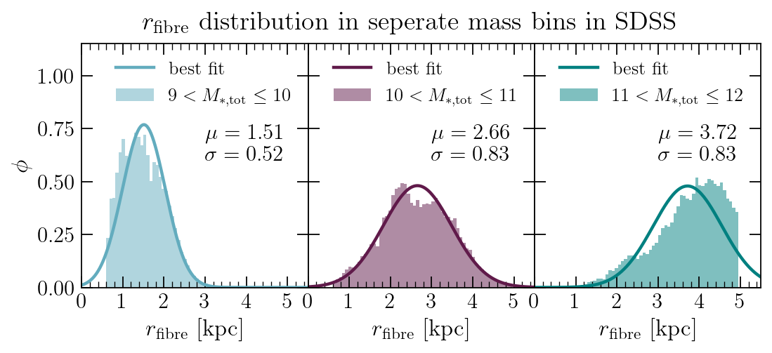
Figure 24: Gaussian fits to fibre radii distributions in the SDSS in bins of stellar mass. Each galaxy in the simulations is assigned a random draw from the fits and relevant quantities are integrated up to this radial extent to check how restricting the simulated results to galactic centres influences raw trends for entire galaxies.

The second step in our observational realism imitates object selection based on emission line fluxes in the SDSS. This sample cut effectively removes objects with low SFR from our sample of observed galaxies, substantially decreasing the size of its quiescent population. In order to apply a similar selection in the simulations we first calculate the sample completeness as a function of $\log({\rm sSFR})$ in the SDSS, once we select the objects based on cuts in S/N ratios on emission line fluxes. In Fig. 25 we present the SDSS completeness as a black solid line, overplotted on the raw SFR distribution in Illustris and TNG. For each simulation we then split the objects into 0.2 dex wide bins in $\log({\rm sSFR})$ and randomly select a fraction of galaxies for further analysis, corresponding to the SDSS completeness in a given bin. As we show in Fig. 25 the drop in SDSS completeness coincides with the low-sSFR tail of the distributions in both simulations, hence this realism step preferentially rids the simulations of their quiescent objects, as we originally expected. Most importantly, we remove all objects with global SFR=0 in the simulations, which form a non-negligible population in TNG.

Figure 25: SDSS sample completeness as function of SFR calculated after imposing an emission line S/N ratio cut, which is overlaid on the distribution of SFR values in the simulations. For each SFR bin, a fraction of galaxies corresponding to the SDSS completeness is drawn at random and only this selected subset of objects is used in further analysis. This step mimics the effect of emission line quality cut in the observations.

As a final step in the simulation post-processing we add random scatter to the data, mimicking measurement uncertainty associated with quantities estimated in the SDSS. As we explain in the main text, for each simulated galaxy we add a random draw from a Gaussian centred on 0, such that a given parameter $X$ is assigned a new value of $\log(X_{\rm new})=\log(X)+N(0,\sigma_{X})$ and $\sigma_{X}$ is the median measurement error on this quantity in the SDSS. In Figs. 26-28 we treat ${M_{\rm BH}}$, ${M_{\ast}}$, $M_{\rm\ast,\,fib}$, SFR, ${\rm SFR_{fib}}$ and $M_{\rm H2,\,fib}$ in this fashion, using $\sigma_{X}$ values listed in Table 6. In the case of SFR (both the in-fibre and global) we only add scatter to star forming objects (i.e. classified according to log(sSFR/${\rm yr^{-1}}$) $>-11$) since we treat SFR values in the quenched SDSS galaxies as upper limits estimated from the strength of D4000.

The second columns in Figs. 26, 27 & 28 show the effect of restricting galaxies to SDSS fibre apertures in the simulations. Overall, this primarily acts to highlight and strengthen trends previously seen in entire galaxies. When we look at Fig. 26, we see that raw $f_{\rm gas}$ (labelled as ‘default’ in the figure) in both simulations show decreasing trends between the star forming and passive populations. These trends are also perfectly recovered in the galactic centres, albeit with significant quantitative differences. In Illustris both the SF and PA galaxies have lower $f_{\rm gas}$ in their cores, however the difference is bigger for the Main Sequence objects (a decrease of 0.58 dex in the median value, in contrast with 0.13 dex in the passive population). In TNG, on the other hand, aperture correction has a dramatic effect on $f_{\rm gas}$, revealing passive galaxies which are overwhelmingly devoid of gas in their centres (the median value of $\log(f_{\rm gas})$ in the PA population is equal to -4.60 dex, in contrast with -1.92 dex in the case of whole galaxies). We see very similar effects of aperture correction on median $f_{\rm gas}$ as a function of ${M_{\rm BH}}$ in Fig. 28 as well, where the pronounced decline in raw $f_{\rm gas}$ in Illustris is only marginally steepened, while the central regions of galaxies in TNG record a dramatic drop in $f_{\rm gas}$ around $\log(M_{\rm BH}/M_{\ast})\sim 8$.

Aperture correction in the simulations also acts to strengthen the trends in SFE seen in the raw data. As demonstrated in Fig. 27, galactic centres of quenched objects in Illustris are rather highly efficient at forming new stars, in contrast with their MS counterparts. With the exception of a few high-${M_{\ast}}$ outliers, galaxies overall classified as passive in the suite are making the most of the limited gas available in their centres. When we then look at the trends in SFE as a function of ${M_{\rm BH}}$ in Fig. 28 we can see that the formerly present turn-off at high-${M_{\rm BH}}$ is no longer present in the galactic centres and that, in fact, the most massive black holes in the sample are associated with the highest SFE values in Illustris. In TNG the trend in SFE goes in the exact opposite direction to Illustris in Fig. 27 and aperture correction steepens it by increasing the median difference between SF and PA populations by 0.2 dex. We also see that the galactic centres in the passive sequence are almost exclusively not star forming at all, reaching the SFE floor value. Similarly, when we look at SFE as function of ${M_{\rm BH}}$ in Fig. 28, galaxies above $\log(M_{\rm BH}/{\rm M_{\odot}})\sim 8$ have zero star formation efficiency and only recover their star-forming ability at the highest black hole masses.

Mimicking S/N ratio cuts in the simulations has straightforward consequences for the results in Figs. 26 and 27. The passive sequence in both Illustris and TNG is significantly less numerous and the majority of outliers in $f_{\rm gas}$ and SFE are removed from the $M_{\ast}-{\rm SFR}$ plane. The median values in PA and SF populations are only slightly affected by this realism step and hence the trends remain virtually unchanged. In Fig. 28 the S/N cut affects primarily galaxies with the highest ${M_{\rm BH}}$, decreasing the scatter around median trends in $f_{\rm gas}$ and SFE at the high black hole mass end.

Figure 26: The influence of all observational realism steps on the raw $f_{\rm gas}$ values extracted from Illustris (top row) and TNG (bottom row) in Fig. 12(b). Colour indicates median $f_{\rm gas}$ in each hexagonal bin, while black contours trace object density in the plane. In both simulations the aperture correction (second column) results in a decrease in $f_{\rm gas}$, however the effect is more pronounced in TNG. Imitating the S/N ratio cut on emission lines (third column) visibly decreases the quenched population, dramatically decreasing its size. Mimicking measurement error by adding scatter to the data (rightmost column) causes the Main Sequence to swell, however the decreasing trend in $f_{\rm gas}$ is preserved well.

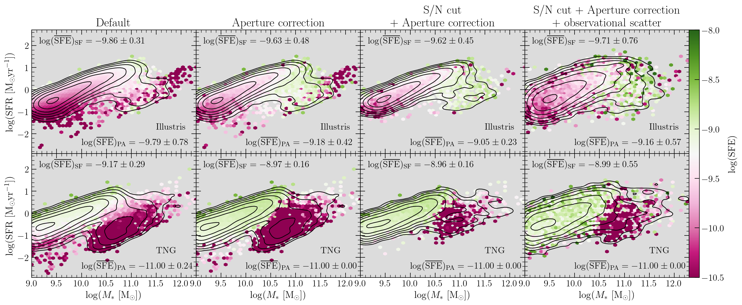
Figure 27: Same as Fig. 26 but with SFE instead of $f_{\rm gas}$. The aperture correction (second column) strongly enhances raw trends in SFE, showing no star formation in galactic centres in TNG and very efficient formation of new stars in Illustris. Adding observation-like scatter and mimicking the S/N ratio cut in the data only further highlights the contrast between Illustris and TNG.

Accounting for measurement error in the simulations preserves all trends seen previously in the $M_{\ast}-{\rm SFR}$ plane, however it has profound consequences for the distribution of galaxies on the star forming Main Sequence. Added scatter significantly spreads out the MS relations in the simulations, causing them to swell and reach down towards the region in the plane occupied by quenched galaxies in the observations. Albeit generous, the random scatter added to raw data is motivated by the observed measurement errors and hence this behaviour of simulated MS might suggest the existence of potential Main Sequence regularisation mechanisms which are not currently captured in cosmological models of structure formation. In Fig. 28 measurement error primarily acts to smoothen median trends in sSFR, $f_{\rm gas}$ and SFE with ${M_{\rm BH}}$, in particular concealing abrupt changes in these quantities in TNG. The difference between the third and fourth columns in the figure suggests an interesting possibility, where even the most dramatic underlying trends in galactic properties could be significantly smeared out by the uncertainty associated with the observations to produce smooth relationships we see in the SDSS.

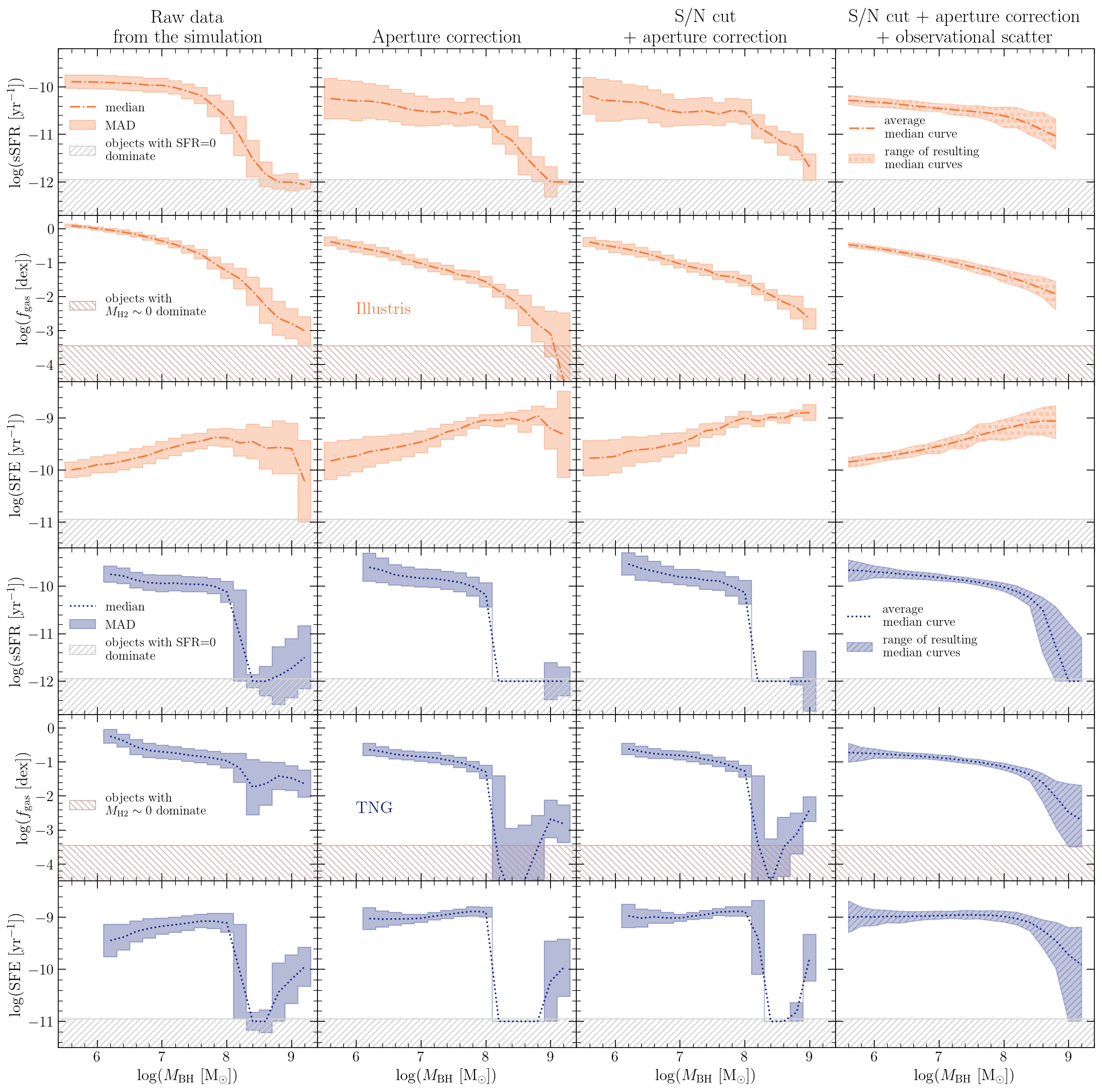
Figure 28: All steps in simulation realism necessary to move between Figs. 14 and 15. As seen previously in Figs. 26 and 27, aperture correction reveals more gas-poor centres in both simulation suites, which are efficiently forming stars in Illustris and are completely deprived of star formation in TNG. Imitating the S/N ratio cut on emission lines in the SDSS affects primarily the quenched population associated with the highest black hole masses in the sample. Adding observation-like measurement uncertainty to the raw data does not have a very strong impact on the median trends in Illustris, while in TNG it acts to smoothen out abrupt drops in sSFR, $f_{\rm gas}$ and SFE around $\log(M_{\rm BH}/{\rm M_{\odot}})\sim 8$.

Appendix E Testing different HI/H₂ transition models

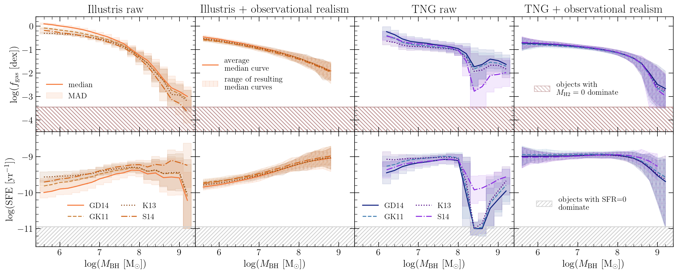
Figure 29: Comparison of$f_{\rm gas}$ and SFE trends among all HI/${\rm H2}$ transition models used to calculate molecular gas fractions in the publicly available HI/H2 galaxy content catalogues. When we focus on the raw output from the simulations we see minimal differences among the models. Once observational realism is included, these differences vanish completely, leaving behind perfectly consistent trends in median quantities.

In order to successfully capture large cosmological volumes within a finite computation tim, simulations need to settle for a relatively low resolution of about a kiloparsec in spatial extent and a million ${\rm M_{\odot}}$ in mass. Moreover, the computational cost associated with including chemical networks and radiative transfer calculations on-the-fly prevents cosmological simulations from tracing the detailed evolution of elements in different phases present within the modelled gas. As a consequence of this limitation, a range of physical properties of gas cannot be directly predicted in a simulation run and requires additional post-processing to extract quantities of interest. An example of such property is the multiphase structure of hydrogen, in particular the abundance of HI and ${\rm H}_{2}$. In order to estimate those in a given simulation snapshot one uses a HI/${\rm H}_{2}$ transition model - a prescription for calculating the fraction of neutral hydrogen in its molecular form given gas state variables, the presence of dust and local ionising radiation. Due to the resolution limit, which is significantly larger than the size of individual molecular clouds in cosmological simulations, these prescriptions depend on locally averaged properties estimated for individual gas cells like e.g. gas metallicity, density or the UV background.

The publicly available HI/${\rm H}_{2}$ catalogues for Illustris and IllustrisTNG (Diemer et al., 2018) contain results obtained using four different models for the HI/${\rm H}_{2}$ transition. The Gnedin & Draine (2014) (GD14) and Gnedin & Kravtsov (2011) (GK11) models are based on high-resolution simulations of isolated disk galaxies, while Krumholz (2013) (K13) and Sternberg et al. (2014) (S14) use analytic prescriptions to compute molecular gas fractions. In this work we present all gas-oriented results using GD14, however we do not have a preference for the choice of model among the available set. For each step in our analysis we also check that the choice of HI/${\rm H}_{2}$transition model does not strongly influence our results and demonstrate this explicitly using median trends in $f_{\rm gas}$ and SFE as an example in Fig. 29.

Fig. 29 presents both the raw results (columns 1 and 3) and simulations post-processed with observational realism (columns 2 and 4) for all four HI/${\rm H}_{2}$transitions models in Illustris and TNG. The top row shows the behaviour of gas fractions, while the bottom one compares the trends in SFE, both as a function of ${M_{\rm BH}}$. It is apparent that the choice of model leads to only very subtle differences in trends inferred from the direct output of the simulations. TS14 deviates most from the other three models and these differences are more striking in SFE in both simulations. They are mainly caused by the differences in galaxy samples among the four curves, because S14 estimates many more objects with $M_{\rm H2}$=0 which also have SFR=0. These need to be removed from the SFE panels because their SFE value is undefined. When we add observational realism to all quantities, however, all minor differences among the models virtually disappear, yielding perfectly consistent median trends in $f_{\rm gas}$ and SFE.

References

- Abazajian et al. (2009) Abazajian K. N., et al., 2009, ApJS, 182, 543
- Aird et al. (2012) Aird J., et al., 2012, ApJ, 746, 90
- Aravena et al. (2019) Aravena M., et al., 2019, ApJ, 882, 136
- Baldry et al. (2004) Baldry I. K., Glazebrook K., Brinkmann J., Ivezić Ž., Lupton R. H., Nichol R. C., Szalay A. S., 2004, ApJ, 600, 681
- Baldry et al. (2006) Baldry I. K., Balogh M. L., Bower R. G., Glazebrook K., Nichol R. C., Bamford S. P., Budavari T., 2006, MNRAS, 373, 469
- Baldwin et al. (1981) Baldwin J. A., Phillips M. M., Terlevich R., 1981, PASP, 93, 5
- Bell et al. (2004) Bell E. F., et al., 2004, ApJ, 608, 752
- Bell et al. (2012) Bell E. F., et al., 2012, ApJ, 753, 167
- Belli et al. (2021) Belli S., et al., 2021, arXiv e-prints, p. arXiv:2102.07881
- Binney (2004) Binney J., 2004, MNRAS, 347, 1093
- Bîrzan et al. (2004) Bîrzan L., Rafferty D. A., McNamara B. R., Wise M. W., Nulsen P. E. J., 2004, ApJ, 607, 800
- Blanton et al. (2005) Blanton M. R., et al., 2005, AJ, 129, 2562
- Bluck et al. (2011) Bluck A. F. L., Conselice C. J., Almaini O., Laird E. S., Nandra K., Grützbauch R., 2011, MNRAS, 410, 1174
- Bluck et al. (2014) Bluck A. F. L., Ellison S. L., Patton D. R., Simard L., Mendel J. T., Teimoorinia H., Moreno J., Starkenburg E., 2014, arXiv e-prints, p. arXiv:1412.3862
- Bluck et al. (2016) Bluck A. F. L., et al., 2016, MNRAS, 462, 2559
- Bluck et al. (2019) Bluck A. F. L., et al., 2019, MNRAS, 485, 666
- Bluck et al. (2020a) Bluck A. F. L., Maiolino R., Sánchez S. F., Ellison S. L., Thorp M. D., Piotrowska J. M., Teimoorinia H., Bundy K. A., 2020a, MNRAS, 492, 96
- Bluck et al. (2020b) Bluck A. F. L., et al., 2020b, MNRAS, 499, 230
- Bluck et al. (2021) Bluck A. F. L., Maiolino R., Brownson S., Conselice C. J., Ellison S. L., Piotrowska J. M., Thorp M. D., submitted, 2021, MNRAS
- Bolatto et al. (2017) Bolatto A. D., et al., 2017, ApJ, 846, 159
- Bondi (1952) Bondi H., 1952, MNRAS, 112, 195
- Bondi & Hoyle (1944) Bondi H., Hoyle F., 1944, MNRAS, 104, 273
- Booth & Schaye (2009) Booth C. M., Schaye J., 2009, MNRAS, 398, 53
- Booth & Schaye (2011) Booth C. M., Schaye J., 2011, MNRAS, 413, 1158
- Bower et al. (2006) Bower R. G., Benson A. J., Malbon R., Helly J. C., Frenk C. S., Baugh C. M., Cole S., Lacey C. G., 2006, MNRAS, 370, 645
- Brammer et al. (2009) Brammer G. B., et al., 2009, ApJ, 706, L173
- Breiman (2001) Breiman L., 2001, Machine Learning, 45, 5
- Brinchmann et al. (2004) Brinchmann J., Charlot S., White S. D. M., Tremonti C., Kauffmann G., Heckman T., Brinkmann J., 2004, MNRAS, 351, 1151
- Bruzual & Charlot (2003) Bruzual G., Charlot S., 2003, MNRAS, 344, 1000
- Bundy et al. (2008) Bundy K., et al., 2008, ApJ, 681, 931
- Cameron & Driver (2009) Cameron E., Driver S. P., 2009, A&A, 493, 489
- Cameron et al. (2009) Cameron E., Driver S. P., Graham A. W., Liske J., 2009, ApJ, 699, 105
- Cardelli et al. (1989) Cardelli J. A., Clayton G. C., Mathis J. S., 1989, ApJ, 345, 245
- Carniani et al. (2015) Carniani S., et al., 2015, A&A, 580, A102
- Colombo et al. (2020) Colombo D., et al., 2020, A&A, 644, A97
- Crain et al. (2015) Crain R. A., et al., 2015, MNRAS, 450, 1937
- Crain et al. (2017) Crain R. A., et al., 2017, MNRAS, 464, 4204
- Crenshaw et al. (2010) Crenshaw D. M., Schmitt H. R., Kraemer S. B., Mushotzky R. F., Dunn J. P., 2010, ApJ, 708, 419
- Croton et al. (2006) Croton D. J., et al., 2006, MNRAS, 365, 11
- Davies et al. (2019) Davies J. J., Crain R. A., McCarthy I. G., Oppenheimer B. D., Schaye J., Schaller M., McAlpine S., 2019, MNRAS, 485, 3783
- Davis & Laor (2011) Davis S. W., Laor A., 2011, ApJ, 728, 98
- Dekel & Birnboim (2006) Dekel A., Birnboim Y., 2006, MNRAS, 368, 2
- Diemer et al. (2018) Diemer B., et al., 2018, ApJS, 238, 33
- Donnari et al. (2021a) Donnari M., et al., 2021a, MNRAS, 500, 4004
- Donnari et al. (2021b) Donnari M., Pillepich A., Nelson D., Marinacci F., Vogelsberger M., Hernquist L., 2021b, MNRAS, 506, 4760
- Dou et al. (2021a) Dou J., et al., 2021a, ApJ, 907, 114
- Dou et al. (2021b) Dou J., et al., 2021b, ApJ, 915, 94
- Dubois et al. (2016) Dubois Y., Peirani S., Pichon C., Devriendt J., Gavazzi R., Welker C., Volonteri M., 2016, MNRAS, 463, 3948
- Ellison et al. (2020) Ellison S. L., et al., 2020, MNRAS, 493, L39
- Ellison et al. (2021) Ellison S. L., Lin L., Thorp M. D., Pan H.-A., Sánchez S. F., Bluck A. F. L., Belfiore F., 2021, MNRAS, 502, L6
- Faber et al. (2007) Faber S. M., et al., 2007, ApJ, 665, 265
- Fabian (2012) Fabian A. C., 2012, ARA&A, 50, 455
- Fawcett (2006) Fawcett T., 2006, Pattern Recognition Letters, 27, 861
- Federrath & Klessen (2012) Federrath C., Klessen R. S., 2012, ApJ, 761, 156
- Feruglio et al. (2010) Feruglio C., Maiolino R., Piconcelli E., Menci N., Aussel H., Lamastra A., Fiore F., 2010, A&A, 518, L155
- Fluetsch et al. (2019) Fluetsch A., et al., 2019, MNRAS, 483, 4586
- Fluetsch et al. (2020) Fluetsch A., et al., 2020, arXiv e-prints, p. arXiv:2006.13232
- Fukazawa et al. (2006) Fukazawa Y., Botoya-Nonesa J. G., Pu J., Ohto A., Kawano N., 2006, ApJ, 636, 698
- Furlong et al. (2015) Furlong M., et al., 2015, MNRAS, 450, 4486
- Genel et al. (2014) Genel S., et al., 2014, MNRAS, 445, 175
- Genel et al. (2018) Genel S., et al., 2018, MNRAS, 474, 3976
- Gensior et al. (2020) Gensior J., Kruijssen J. M. D., Keller B. W., 2020, MNRAS, 495, 199
- Genzel et al. (2015) Genzel R., et al., 2015, ApJ, 800, 20
- Georgakakis et al. (2008) Georgakakis A., et al., 2008, MNRAS, 385, 2049
- Giallongo et al. (2005) Giallongo E., Salimbeni S., Menci N., Zamorani G., Fontana A., Dickinson M., Cristiani S., Pozzetti L., 2005, ApJ, 622, 116
- Gnedin & Draine (2014) Gnedin N. Y., Draine B. T., 2014, ApJ, 795, 37
- Gnedin & Kravtsov (2011) Gnedin N. Y., Kravtsov A. V., 2011, ApJ, 728, 88
- Gudennavar et al. (2012) Gudennavar S. B., Bubbly S. G., Preethi K., Murthy J., 2012, ApJS, 199, 8
- Häring & Rix (2004) Häring N., Rix H.-W., 2004, ApJ, 604, L89
- Harrison et al. (2014) Harrison C. M., Alexander D. M., Mullaney J. R., Swinbank A. M., 2014, MNRAS, 441, 3306
- Harrison et al. (2019) Harrison C. M., Alexander D. M., Rosario D. J., Scholtz J., Stanley F., 2019, arXiv e-prints, p. arXiv:1912.01020
- Hastie et al. (2009) Hastie T., Tibshirani R., Friedman J., 2009, The Elements of Statistical Learning (2nd edition). Springer-Verlag
- Heckman & Best (2014) Heckman T. M., Best P. N., 2014, ARA&A, 52, 589
- Heinz et al. (1998) Heinz S., Reynolds C. S., Begelman M. C., 1998, ApJ, 501, 126
- Henriques et al. (2019) Henriques B. M. B., White S. D. M., Lilly S. J., Bell E. F., Bluck A. F. L., Terrazas B. A., 2019, MNRAS, 485, 3446
- Hickox et al. (2009) Hickox R. C., et al., 2009, ApJ, 696, 891
- Hinshaw et al. (2013) Hinshaw G., et al., 2013, ApJS, 208, 19
- Hlavacek-Larrondo et al. (2012) Hlavacek-Larrondo J., Fabian A. C., Edge A. C., Ebeling H., Sanders J. S., Hogan M. T., Taylor G. B., 2012, MNRAS, 421, 1360
- Hlavacek-Larrondo et al. (2015) Hlavacek-Larrondo J., et al., 2015, ApJ, 805, 35
- Hopkins & Elvis (2010) Hopkins P. F., Elvis M., 2010, MNRAS, 401, 7
- Hopkins et al. (2007) Hopkins P. F., Hernquist L., Cox T. J., Robertson B., Krause E., 2007, ApJ, 669, 67
- Hopkins et al. (2008) Hopkins P. F., Hernquist L., Cox T. J., Kereš D., 2008, ApJS, 175, 356
- Hopkins et al. (2011) Hopkins P. F., Quataert E., Murray N., 2011, MNRAS, 417, 950
- Hoyle & Lyttleton (1939) Hoyle F., Lyttleton R. A., 1939, Proceedings of the Cambridge Philosophical Society, 35, 405
- Hummer & Storey (1987) Hummer D. G., Storey P. J., 1987, MNRAS, 224, 801
- Humphrey et al. (2011) Humphrey P. J., Buote D. A., Canizares C. R., Fabian A. C., Miller J. M., 2011, ApJ, 729, 53
- Jorgensen et al. (1995) Jorgensen I., Franx M., Kjaergaard P., 1995, MNRAS, 276, 1341
- Kauffmann et al. (2003) Kauffmann G., et al., 2003, MNRAS, 341, 33
- Kay et al. (2002) Kay S. T., Pearce F. R., Frenk C. S., Jenkins A., 2002, MNRAS, 330, 113
- Kendall & Stuart (1977) Kendall M. G., Stuart A., 1977, The Advanced Theory of Statistics: Inference and Relationship. (vol 2). London : C. Griffin
- Kormendy & Ho (2013) Kormendy J., Ho L. C., 2013, ARA&A, 51, 511
- Kormendy et al. (2011) Kormendy J., Bender R., Cornell M. E., 2011, Nature, 469, 374
- Krumholz (2013) Krumholz M. R., 2013, MNRAS, 436, 2747
- Krumholz & McKee (2005) Krumholz M. R., McKee C. F., 2005, ApJ, 630, 250
- Kumari et al. (2019) Kumari N., Maiolino R., Belfiore F., Curti M., 2019, MNRAS, 485, 367
- Lim et al. (2017) Lim S. H., Mo H. J., Lan T. W., Ménard B., 2017, MNRAS, 464, 3256
- Lin et al. (2017) Lin L., et al., 2017, ApJ, 851, 18
- Lin et al. (2020) Lin L., et al., 2020, ApJ, 903, 145
- Liu et al. (2019) Liu C., Hao L., Wang H., Yang X., 2019, ApJ, 878, 69
- Louppe (2014) Louppe G., 2014, arXiv e-prints, p. arXiv:1407.7502
- Maiolino et al. (2012) Maiolino R., et al., 2012, MNRAS, 425, L66
- Malmquist (1922) Malmquist K. G., 1922, Meddelanden fran Lunds Astronomiska Observatorium Serie I, 100, 1
- Maraston & Strömbäck (2011) Maraston C., Strömbäck G., 2011, MNRAS, 418, 2785
- Marinacci et al. (2018) Marinacci F., et al., 2018, MNRAS, 480, 5113
- Marri & White (2003) Marri S., White S. D. M., 2003, MNRAS, 345, 561
- Martig et al. (2009) Martig M., Bournaud F., Teyssier R., Dekel A., 2009, ApJ, 707, 250
- Martín-Navarro et al. (2018) Martín-Navarro I., Brodie J. P., Romanowsky A. J., Ruiz-Lara T., van de Ven G., 2018, Nature, 553, 307
- Mathur et al. (2012) Mathur S., Fields D., Peterson B. M., Grupe D., 2012, ApJ, 754, 146
- McAlpine et al. (2016) McAlpine S., et al., 2016, Astronomy and Computing, 15, 72
- McCarthy et al. (2011) McCarthy I. G., Schaye J., Bower R. G., Ponman T. J., Booth C. M., Dalla Vecchia C., Springel V., 2011, MNRAS, 412, 1965
- McConnell & Ma (2013) McConnell N. J., Ma C.-P., 2013, ApJ, 764, 184
- McNamara & Nulsen (2007) McNamara B. R., Nulsen P. E. J., 2007, ARA&A, 45, 117
- McNamara et al. (2000) McNamara B. R., et al., 2000, ApJ, 534, L135
- Mendel et al. (2014) Mendel J. T., Simard L., Palmer M., Ellison S. L., Patton D. R., 2014, ApJS, 210, 3
- Misner et al. (1973) Misner C. W., Thorne K. S., Wheeler J. A., 1973, Gravitation
- Naiman et al. (2018) Naiman J. P., et al., 2018, MNRAS, 477, 1206
- Nandra et al. (2007) Nandra K., et al., 2007, ApJ, 660, L11
- Nelson et al. (2015) Nelson D., et al., 2015, Astronomy and Computing, 13, 12
- Nelson et al. (2018) Nelson D., et al., 2018, MNRAS, 475, 624
- Nelson et al. (2019) Nelson D., et al., 2019, Computational Astrophysics and Cosmology, 6, 2
- Nelson et al. (2021) Nelson E. J., et al., 2021, MNRAS,
- Noeske et al. (2007) Noeske K. G., et al., 2007, ApJ, 660, L43
- Omand et al. (2014) Omand C. M. B., Balogh M. L., Poggianti B. M., 2014, MNRAS, 440, 843
- Paolillo et al. (2002) Paolillo M., Fabbiano G., Peres G., Kim D. W., 2002, ApJ, 565, 883
- Pawlowski & Kroupa (2020) Pawlowski M. S., Kroupa P., 2020, MNRAS, 491, 3042
- Pedregosa et al. (2011) Pedregosa F., et al., 2011, Journal of Machine Learning Research, 12, 2825
- Peng & Renzini (2020) Peng Y.-j., Renzini A., 2020, MNRAS, 491, L51
- Peng et al. (2010) Peng Y.-j., et al., 2010, ApJ, 721, 193
- Peng et al. (2012) Peng Y.-j., Lilly S. J., Renzini A., Carollo M., 2012, ApJ, 757, 4
- Pillepich et al. (2018a) Pillepich A., et al., 2018a, MNRAS, 473, 4077
- Pillepich et al. (2018b) Pillepich A., et al., 2018b, MNRAS, 475, 648
- Piotrowska et al. (2020) Piotrowska J. M., Bluck A. F. L., Maiolino R., Concas A., Peng Y., 2020, MNRAS, 492, L6
- Planck Collaboration et al. (2014) Planck Collaboration et al., 2014, A&A, 571, A1
- Pontzen et al. (2017) Pontzen A., Tremmel M., Roth N., Peiris H. V., Saintonge A., Volonteri M., Quinn T., Governato F., 2017, MNRAS, 465, 547
- Reines & Volonteri (2015) Reines A. E., Volonteri M., 2015, ApJ, 813, 82
- Renzini (2020) Renzini A., 2020, MNRAS, 495, L42
- Renzini & Peng (2015) Renzini A., Peng Y.-j., 2015, ApJ, 801, L29
- Rosario et al. (2013) Rosario D. J., et al., 2013, ApJ, 771, 63
- Rosas-Guevara et al. (2015) Rosas-Guevara Y. M., et al., 2015, MNRAS, 454, 1038
- Rupke et al. (2017) Rupke D. S. N., Gültekin K., Veilleux S., 2017, ApJ, 850, 40
- Saglia et al. (2016) Saglia R. P., et al., 2016, ApJ, 818, 47
- Saintonge et al. (2017) Saintonge A., et al., 2017, ApJS, 233, 22
- Saintonge et al. (2018) Saintonge A., et al., 2018, MNRAS, 481, 3497
- Salim et al. (2007) Salim S., et al., 2007, ApJS, 173, 267
- Santini et al. (2009) Santini P., et al., 2009, A&A, 504, 751
- Scannapieco & Oh (2004) Scannapieco E., Oh S. P., 2004, ApJ, 608, 62
- Schaye et al. (2015) Schaye J., et al., 2015, MNRAS, 446, 521
- Shakura & Sunyaev (1973) Shakura N. I., Sunyaev R. A., 1973, A&A, 500, 33
- Shankar et al. (2009) Shankar F., Weinberg D. H., Miralda-Escudé J., 2009, ApJ, 690, 20
- Sijacki et al. (2007) Sijacki D., Springel V., Di Matteo T., Hernquist L., 2007, MNRAS, 380, 877
- Sijacki et al. (2015) Sijacki D., Vogelsberger M., Genel S., Springel V., Torrey P., Snyder G. F., Nelson D., Hernquist L., 2015, MNRAS, 452, 575
- Silk & Rees (1998) Silk J., Rees M. J., 1998, A&A, 331, L1
- Simard et al. (2011) Simard L., Mendel J. T., Patton D. R., Ellison S. L., McConnachie A. W., 2011, ApJS, 196, 11
- Snyder et al. (2015) Snyder G. F., et al., 2015, MNRAS, 454, 1886
- Somerville & Davé (2015) Somerville R. S., Davé R., 2015, ARA&A, 53, 51
- Sorai et al. (2019) Sorai K., et al., 2019, PASJ, 71, S14
- Sparre et al. (2015) Sparre M., et al., 2015, MNRAS, 447, 3548
- Springel (2005) Springel V., 2005, MNRAS, 364, 1105
- Springel (2010) Springel V., 2010, MNRAS, 401, 791
- Springel & Hernquist (2003) Springel V., Hernquist L., 2003, MNRAS, 339, 289
- Springel et al. (2018) Springel V., et al., 2018, MNRAS, 475, 676
- Sternberg et al. (2014) Sternberg A., Le Petit F., Roueff E., Le Bourlot J., 2014, ApJ, 790, 10
- Strateva et al. (2001) Strateva I., et al., 2001, AJ, 122, 1861
- Tacconi et al. (2018) Tacconi L. J., et al., 2018, ApJ, 853, 179
- Tal et al. (2014) Tal T., et al., 2014, ApJ, 789, 164
- Taylor et al. (2016) Taylor C., Boylan-Kolchin M., Torrey P., Vogelsberger M., Hernquist L., 2016, MNRAS, 461, 3483
- Teimoorinia et al. (2016) Teimoorinia H., Bluck A. F. L., Ellison S. L., 2016, MNRAS, 457, 2086
- Terrazas et al. (2016) Terrazas B. A., Bell E. F., Henriques B. M. B., White S. D. M., Cattaneo A., Woo J., 2016, ApJ, 830, L12
- Terrazas et al. (2017) Terrazas B. A., Bell E. F., Woo J., Henriques B. M. B., 2017, ApJ, 844, 170
- Terrazas et al. (2020) Terrazas B. A., et al., 2020, MNRAS, 493, 1888
- Trayford et al. (2015) Trayford J. W., et al., 2015, MNRAS, 452, 2879
- Trump et al. (2015) Trump J. R., et al., 2015, ApJ, 811, 26
- Veilleux et al. (2013) Veilleux S., et al., 2013, ApJ, 776, 27
- Venturi et al. (2021) Venturi G., et al., 2021, A&A, 648, A17
- Villar-Martín et al. (2011) Villar-Martín M., Humphrey A., Delgado R. G., Colina L., Arribas S., 2011, MNRAS, 418, 2032
- Vogelsberger et al. (2014a) Vogelsberger M., et al., 2014a, MNRAS, 444, 1518
- Vogelsberger et al. (2014b) Vogelsberger M., et al., 2014b, Nature, 509, 177
- Wake et al. (2012) Wake D. A., van Dokkum P. G., Franx M., 2012, ApJ, 751, L44
- Wang et al. (2018) Wang H., et al., 2018, ApJ, 852, 31
- Wang et al. (2020) Wang B., Cappellari M., Peng Y., Graham M., 2020, MNRAS, 495, 1958
- Weinberger et al. (2017) Weinberger R., et al., 2017, MNRAS, 465, 3291
- Weinberger et al. (2018) Weinberger R., et al., 2018, MNRAS, 479, 4056
- Werner et al. (2019) Werner N., McNamara B. R., Churazov E., Scannapieco E., 2019, Space Sci. Rev., 215, 5
- Willmer et al. (2006) Willmer C. N. A., et al., 2006, ApJ, 647, 853
- Woo et al. (2013) Woo J., et al., 2013, MNRAS, 428, 3306
- Woo et al. (2015) Woo J., Dekel A., Faber S. M., Koo D. C., 2015, MNRAS, 448, 237
- Wu et al. (2013) Wu S., Lu Y., Zhang F., Lu Y., 2013, MNRAS, 436, 3271
- Wyder et al. (2007) Wyder T. K., et al., 2007, ApJS, 173, 293
- Xue et al. (2010) Xue Y. Q., et al., 2010, ApJ, 720, 368
- Yang et al. (2007) Yang X., Mo H. J., van den Bosch F. C., Pasquali A., Li C., Barden M., 2007, ApJ, 671, 153
- Yang et al. (2009) Yang X., Mo H. J., van den Bosch F. C., 2009, ApJ, 695, 900
- York et al. (2000) York D. G., et al., 2000, AJ, 120, 1579
- Zakamska & Greene (2014) Zakamska N. L., Greene J. E., 2014, MNRAS, 442, 784
- Zhu et al. (2018) Zhu Q., et al., 2018, MNRAS, 480, L18
- Zinger et al. (2020) Zinger E., et al., 2020, MNRAS, 499, 768
- van den Bosch et al. (2008) van den Bosch F. C., Aquino D., Yang X., Mo H. J., Pasquali A., McIntosh D. H., Weinmann S. M., Kang X., 2008, MNRAS, 387, 79