AI and extreme scale computing to learn and infer the physics of higher order gravitational wave modes of quasi-circular, spinning, non-precessing black hole mergers

Abstract

We use artificial intelligence (AI) to learn and infer the physics of higher order gravitational wave modes of quasi-circular, spinning, non precessing binary black hole mergers. We trained AI models using 14 million waveforms, produced with the surrogate model NRHybSur3dq8, that include modes up to $\ell\leq 4$ and $(5,5)$, except for $(4,0)$ and $(4,1)$, that describe binaries with mass-ratios $q\leq 8$, individual spins $s^{z}_{\{1,2\}}\in[-0.8,0.8]$, and inclination angle $\theta\in[0,\pi]$. Our probabilistic AI surrogates can accurately constrain the mass-ratio, individual spins, effective spin, and inclination angle of numerical relativity waveforms that describe such signal manifold. We compared the predictions of our AI models with Gaussian process regression, random forest, k-nearest neighbors, and linear regression, and with traditional Bayesian inference methods through the PyCBC Inference toolkit, finding that AI outperforms all these approaches in terms of accuracy, and are between three to four orders of magnitude faster than traditional Bayesian inference methods. Our AI surrogates were trained within 3.4 hours using distributed training on 1,536 NVIDIA V100 GPUs in the Summit supercomputer.

Keywords: AI, Black Holes, High Performance Computing, Higher-order Waveform Modes

1 Introduction

The development of rigorous, reproducible, statistically and domain informed artificial intelligence (AI) is leading to remarkable breakthroughs in science and engineering  [1], and guiding human intuition to find new fundamental results in pure mathematics [2]. AI applications in gravitational wave astrophysics are evolving from prototypes to production scale discovery frameworks. Since we developed the first AI models to create a scalable, computationally efficient method to search for and find gravitational waves [3, 4], this approach has been embraced and further developed by an international community of researchers [5, 6, 7]. To date, AI has been explored for a variety of signal processing tasks, including detection [8, 9, 10, 11, 12, 13, 14, 15, 16, 17, 18, 19, 20, 21, 22, 23, 24], gravitational wave denoising and data cleaning [25, 26, 27], parameter estimation [28, 29, 30, 31, 32, 33, 34], rapid waveform production [35, 36], waveform forecasting [37, 38], and early warning systems for multi-messenger sources [39, 40, 41], including the modeling of multi-scale and multi-physics systems [42, 43, 44], among others.

Production scale AI frameworks for gravitational wave detection that harness high performance computing (HPC) and scientific data infrastructure have also been developed [45, 46], furnishing evidence for the scalability, reproducibility and computational efficiency of AI-driven methodologies [47]. Figure 1 provides a glimpse of the rapid convergence of AI and extreme scale computing to study astrophysical scenarios that require waveforms with richer and more complex morphology. In view of these developments, it is time to further push the frontiers of AI applications to quantify their suitability to describe high-dimensional signal manifolds that contain waveforms whose morphology is significantly richer and much more complex than what has already been explored in the literature. This article represents a step in that direction. The driver we have selected for this study consists of characterizing higher order gravitational wave modes emitted by quasi-circular, spinning, non-precessing binary black hole mergers. We densely sample a parameter space that consists of binaries with mass-ratios $q\leq 8$, individual spins $s^{z}_{\{1,2\}}\in[-0.8,0.8]$, and inclination angle $\theta\in[0,\pi]$ using a training dataset of 14M waveforms. The sheer size of this training dataset requires the combination of AI and HPC, and thus we harnessed the Summit supercomputer at Oak Ridge National Laboratory to reduce the training stage from months (using a single V100 GPU) to 3.4 hours using distributed training over 1536 NVIDIA V100 GPUs.

While this article showcases the convergence of AI and HPC for a computational grand challenge, the main goal of this analysis is to explore what new insights we may obtain by conducting AI-driven studies of the signal manifold of higher order gravitational wave modes. In particular, in this article we aim to explore the following open questions [48]:

1. Is it possible for AI to learn and accurately characterize the physics of high-dimensional gravitational wave signal manifolds?

2. Is it possible to exploit the computational efficiency and scalability of AI to train models with tens of millions of modeled waveforms and conduct fast data-driven analyses with fully trained AI models?

3. Is it true that probabilistic AI models provide more accurate inference predictions when we combine extreme scale computing to reduce time to insight, physics-informed AI architectures and optimization schemes to accelerate convergence, and high dimensional signal manifolds that include higher order wave modes to expose AI models to features and patterns that provide a detailed description of the waveform dynamics of black hole mergers?

4. What insights do we gain when we characterize gravitational wave signal manifolds with waveforms with complex morphology?

As we describe below, the answer to questions 1-3 above is a resounding YES. In terms of new insights, we find that our deterministic and probabilistic AI models provide informative constraints for the mass-ratio, individual spins and inclination angle of higher order waveform modes. These are important results, since our previous work [48] showed that, when we only consider $\ell=|m|=2$ modes, it was difficult to constrain the individual spins of comparable mass-ratio systems, as well as the spin of the secondary for asymmetric mass-ratio systems. This study shows that the inclusion of higher order modes alleviates these problems, and provides an informed description of the ability of AI to characterize this high dimensional signal manifold. Throughout this paper we use geometric units in which $G=c=1$.

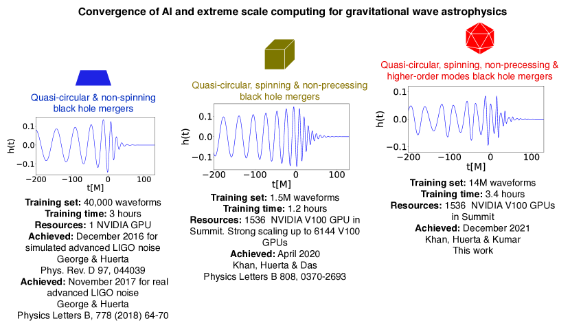
Figure 1: Convergence of AI and extreme scale computing Progress harnessing AI and high performance computing to learn and describe the physics of gravitational wave signal manifolds. A signal manifold with richer complexity (from left to right) provides new opportunities to combine TB-size training datasets with extreme scale computing, allowing the development of novel distributed training algorithms and optimization schemes that incorporate physics and maths principles to accelerate the convergence and performance of AI surrogates.

This paper is organized as follows. Section 2 describes the approach used to create our AI models. We present and discuss our findings in Section 3. Future directions of work are outlined in Section 4.

2 Methods

Here we describe the datasets, AI architectures and training methods followed to create our AI models.

Datasets We use the surrogate model NRHybSur3dq8 [49] to generate time-series datasets that include both the plus, $h_{+}$, and cross, $h_{\times}$, polarizations. These may be represented as a complex time-series $h=h_{+}-ih_{\times}$. $h$ may also be expressed as a sum of spin-weighted spherical harmonic modes, $\mathpzc{h}_{\ell m}$, on the 2-sphere [50]

$$h(t,\theta,\phi_{0})=\sum^{\infty}_{\ell=2}\sum_{m=-l}^{l}\mathpzc{h}_{\ell m}(t)~{}^{-2}Y_{\ell m}(\theta,\phi_{0}),$$ (1)

where ${}^{-2}Y_{\ell m}$ are the spin-weight $\!\!-2$ spherical harmonics, $\theta$ is the inclination angle between the orbital angular momentum of the binary and line of sight to the detector, and $\phi_{0}$ is the initial binary phase, that we set to zero in this study. Our waveforms include higher order modes with $\ell\leq 4$ and $(\ell,m)=(5,5)$, excluding the $(\ell,m)=(4,0)$ and $(4,1)$ modes; cover the time span $t\in[-10,000\,\textrm{M},130\,\textrm{M}]$ with the merger peak occurring at $t=0M$; and are sampled with a time step $\Delta t=1\,\textrm{M}$. Figure 2 presents a sample of waveforms that help visualize the importance of including higher order modes in terms of the amplitude and phase evolution, as well as the morphology of the ringdown phase. The top panel presents a waveform signal that only includes the $\ell=|m|=2$ mode at an optimally oriented configuration, $\theta=0$, that maximizes the amplitude of the signal for detectability purposes. The bottom panels show what new information may be obtained as we construct waveform signals that include higher order modes, i.e., the amplitude and phase of the pre-merger waveform signal exhibits novel, non-linear features as well as a richer and much more complex ringdown phase. In stark contrast, the top panel will only change the amplitude of the waveform signal for angles $\theta=\{\pi/4,\pi/2\}$, since the $\ell=|m|=2$ mode signal is modulated by a constant multiplicative factor that is set by the inclination angle [51, 52].

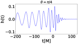
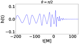
Figure 2: Impact of higher order modes. For a binary black hole merger with parameters $\{q,s_{1}^{z},s_{2}^{z}\}=\{7.05,0.77,0.77\}$, we show waveforms with $(l=|m|=2;\theta=0)$ (top panel), and waveforms including higher order modes up to $\ell\leq 4$ and $(5,5)$, excluding the $(4,0)$ and $(4,1)$ modes, for $\theta=\{0,\pi/4,\pi/2\}$ (bottom panels).

Training dataset It consists of $\sim 14$ million waveforms that cover a 4-D parameter space that encompasses mass-ratio, individual spins and inclination angle $\{q,s_{1}^{z},s_{2}^{z},\theta\}$, respectively. We generate it by sampling the mass-ratio $q\in[1,8]$ in steps of $\Delta q=0.1$; individual spins $s^{z}_{i}\in[-0.8,0.8]$ in steps of $\Delta s^{z}_{i}=0.02$; and the inclination angle $\theta\in[0,\pi]$ in steps of $\Delta\theta=0.1$.

Validation and test datasets Each of these sets consist of $\sim 800,000$ waveforms, and are generated by alternately sampling values that are inbetween the training set values.

AI architecture We use a slightly modified WaveNet [53] neural network architecture for our model. WaveNet’s main features that are relevant for this work include dilated causal convolutions, gated activation units, and the usage of residual and skip connections. These features help capture long range correlations in the input time-series, and facilitate the training of deeper neural networks. Furthermore, since we are interested in regression analyses, we turn off the causal padding in the convolutional layers. We use a filter size of 2 in all convolutional layers and stack 3 residual blocks each consisting of 14 dilated convolutions. For a more in depth discussion of the architecture we refer the reader to [48, 53]. The output from the WaveNet is then fed into three separate branches of fully-connected layers. Each branch is trained to predict the mass ratio, $q$, the effective spin parameters, $(S_{\textrm{eff}}$, $\sigma_{\textrm{eff}})$, and the inclination angle, $\theta$, respectively, where

$$S_{\textrm{eff}}=\sigma_{1}s^{z}_{1}+\sigma_{2}s^{z}_{2}\,,\quad\textrm{with}\quad\sigma_{1}\equiv 1+\frac{3}{4q}\quad\textrm{and}\quad\sigma_{2}\equiv 1+\frac{3q}{4}\,,$$ (2)

$$\textrm{and}\quad\sigma_{\textrm{eff}}=\frac{m_{1}s^{z}_{1}+m_{2}s^{z}_{2}}{m_{1}+m_{2}}=\frac{qs^{z}_{1}+s^{z}_{2}}{1+q}\,.$$ (3)

Since our goal is to predict $\{q,s^{z}_{1},s^{z}_{2},\theta\}$, we solve Eqs. (2) and (3) in conjunction with the predicted $q$ values in order to extract the individual spins $s^{z}_{i}$.

Training methodology We employ mean-squared error (MSE) between the predicted and the ground-truth values as the loss function. During training, we monitor the loss on the validation set to dynamically reduce learning rate as well as to stop training before over-fitting. We reduce the learning rate by a factor of $2$ whenever the validation loss does not decrease for $3$ consecutive epochs, and stop the training when the validation loss does not decrease for $5$ consecutive epochs. Training the model on $256$ nodes, equivalent to 1,536 NVIDIA V100 GPUs, in the Summit Supercomputer then takes about $71$ epochs, using LAMB [54] optimizer with initial learning rate set to $0.001$.

Normalizing Flow: In addition to the above analysis for point estimates, we also trained a normalizing flow model to estimate the posterior distribution. To do that, instead of extracting the parameters directly, we use the WaveNet model as a feature extractor and then condition a normalizing flow model on the extracted features to estimate the posterior distribution. This method was first delineated in [55], and then used in other studies [28, 33]. We follow the same procedure, making use of the nflows library [56]. Normalizing flow is an example of a “likelihood-free” inference method, and is made up of a composition of invertible maps to transform a simple base probability distribution (e.g., a multivariate Gaussian) into a desired posterior distribution which could be very complicated. The transformed distribution is then given by the change of variable formula:

$$p_{X}(x)=p_{Z}(z)\left|\det[\mathbf{J}_{f}(z)]\right|^{-1}\,,$$ (4)

where $Z$ is the random variable for the base distribution, $X$ is the random variable for the transformed distribution, and $f$ is the normalizing flow (i.e., the invertible transformation), such that $X=f(Z)$. In our case, the goal is to model the conditional posterior distribution $p(y|h)$ for the parameters $y$ corresponding to the waveform strain $h$. We do this in two steps (as illustrated in Figure 3); first we pass the strain $h$ through the WaveNet model to extract a feature vector $\tilde{h}$. We then use a conditional version of normalizing flow $f_{\tilde{h},\vartheta}$, specifically a neural spline flow [57], to transform the base Standard Multivariate Gaussian $\mathcal{N}(\mu=0,\Sigma=\mathbf{I})$ to the predicted posterior distribution $q(y|h)$. The function $f_{\tilde{h},\vartheta}$ therefore depends on the input waveform $h$ (through the feature vector $\tilde{h}$), and is parameterized by learnable weights $\vartheta$. The normalizing flow model is then trained by updating the parameter $\vartheta$ so that predicted distribution $q(y|h)$ matches the true posterior distribution $p(y|h)$. This is achieved by minimizing the negative log-likelihood, i.e., given a batch of $N$ ground-truth parameters $y_{i}$ and their corresponding waveforms $h_{i}$, the objective for the normalizing flow model is to minimize:

$$L=-\frac{1}{N}\sum_{i=1}^{N}\log q(y_{i}|h_{i})$$ (5)

where, according to Equation 4;

$$q(y_{i}|h_{i})=p_{\mathcal{N}}(z)\left|\det[\mathbf{J}_{f_{\tilde{h},\theta}}(z)]\right|^{-1}\,.$$ (6)

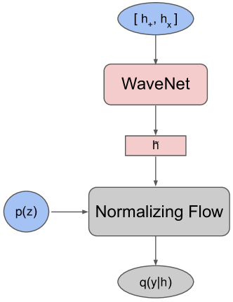
Figure 3: Normalizing flow model architecture. Schematic representation that indicates how we feed the waveform $[h_{+},h_{x}]$ into a WaveNet model to extract the feature vector $\tilde{h}$. Then the normalizing flow $f_{\tilde{h},\theta}$ takes in this feature vector and transforms the base distribution $\mathcal{N}(\mu=0,\Sigma=\mathbf{I})$ into the predicted posterior distribution $q(y|h)$.

3 Results

We present results using deterministic and probabilistic AI models, which we described in Section 2. As described above, these AI models have been designed to take in time-series waveform signals that includes both polarizations $(h_{+},h_{\times})$, and then output the most likely values for $\{q,s_{1}^{z},s_{2}^{z},\theta\}$ that best reproduce the input signal.

3.1 Deterministic AI models

In Figure 4 we provide a sample of results of the predictive capabilities of our deterministic AI models for a variety of input waveform signals. Note that ground truth waveforms are shown in blue, whereas waveforms whose parameters, $\{q,s_{1}^{z},s_{2}^{z},\theta\}$, are predicted by AI are shown in dotted red. We quantify the accuracy of our AI models by computing the overlap, ${\cal{O}}(h_{t}|h_{p})$, between ground-truth, $h_{t}$, and AI-predicted, $h_{p}$, waveforms using

$${\cal{O}}(h_{t}|h_{p})=\underset{[t_{c}\,\phi_{c}]}{\mathrm{max}}\left(\hat{h}_{t}|\hat{h}_{p}{[t_{c},\,\phi_{c}]}\right)\,,\quad{\rm with}\quad\hat{h}_{t}=h_{t}\,\left(h_{t}|h_{t}\right)^{-1/2}\,,$$ (7)

where ${[t_{c},\,\phi_{c}]}$ are the amounts by which the normalized waveform $\hat{h}_{p}$ has been time- and phase-shifted.

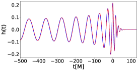
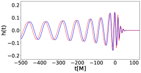
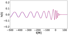
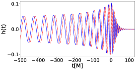
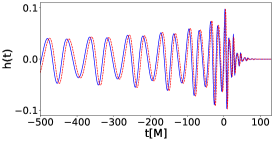
Figure 4: Comparison between ground truth and AI-predicted waveforms Ground truth waveforms (in blue) and AI predicted waveforms (dotted red). Top panels: $\{q,s_{1}^{z},s_{2}^{z}\}=\{2.05,-0.79,0.77\}$, bottom panels: $\{q,s_{1}^{z},s_{2}^{z}\}=\{7.85,0.77,-0.79\}$. We show waveforms, from left to right, with inclination angles $\theta=\{0,\pi/4,\pi/2\}$. In all these cases, the overlap between ground truth and predicted waveforms is ${\cal{O}}\geq 0.98$.

Figure 5 summarizes the accuracy with which deterministic AI models estimate the parameters of higher order modes for all mass-ratios and spins for a sample of inclination angles. There we notice that predictions degrade in accuracy for edge-on systems, i.e., $\theta=\pi/2$. Note that a mild shift is seen in the predicted values of the inclination angle, $\theta$, from its ground truth value in panels with $\theta=\{0,\pi\}$, although the distribution has the true value well within a $1-\sigma$ deviation from its median. This shift is likely because $0$ and $\pi$ correspond to the domain boundary of $\theta$ as $0\leq\theta<\pi$, which leads to a one-sided wrap-around of the recovered distribution of $\theta$ values, and in turn leads to a shift in the median recovered value toward the boundary. We provide a more comprehensive analysis of these results in Figure 6, where we show overlap calculations between ground truth and predicted signals in terms of symmetric mass-ratio and effective spin $(\eta,\sigma_{\mathrm{eff}})$ for all mass-ratios and spins under consideration for a sample of inclination angles. Again, here we find that our results are optimal for all angles except for edge-on binaries. We can understand this if we recall that for $\theta=\pi/2$ we lose half of the information we feed into our AI models since $h_{\times}\left(t,\theta=\pi/2\right)\rightarrow 0$. In summary, our deterministic AI models provide informative point parameter estimation results for the parameter space under consideration.

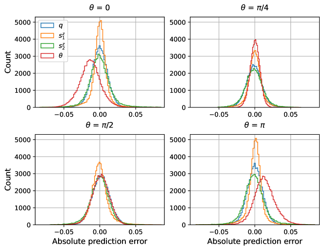
Figure 5: Statistical results of deterministic AI models Absolute errors for all mass ratios, $q$, and individual spins, $(s_{1}^{z},s_{2}^{z})$, for a sample of inclination angles. The true values of inclination angles are $[0.054,0.70,1.57,3.09]$ and are rounded-off for labeling above.

Figure 6: Overlap between ground truth signals and those predicted by deterministic AI models Overlap between ground truth and AI-predicted signals in terms of symmetric mass-ratio, $\eta$, and effective spin, $\sigma_{\mathrm{eff}}$, for a sample of inclination angles.

3.2 Comparison to other machine learning methods

We have compared the predictions of our AI models with other machine learning algorithms, including, Gaussian Process Regression, Random Forest, k-Nearest Neighbors and Linear Regression. The results of this analysis are shown shown in Figure 7.

For this comparison, we had to reduce the amount of training data, since traditional machine learning models are sub-optimal to handle the TB-size training datasets used to train our AI models. Thus, we considered a reduced data set that describes black hole binaries with mass-ratios $q\in\{4.0,4.1\}$ and inclination angles $\theta\in\{0.0,0.1\}$, and all possible spin combinations. Then, we tested these machine learning models on a test set with $q=4.05$ and $\theta=0.05$, and all possible spin combinations. Using the same metric we have considered above to quantify the performance of our AI models, e.g., mean absolute error, Figure 7 presents the average absolute errors over all four parameters under consideration, $(q,s_{1}^{z},s_{2}^{z},\theta)$. It is apparent that even in this scenario that provides a clear advantage to traditional machine learning models, neural networks still provide better results.

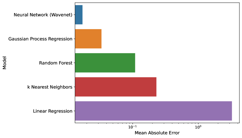
Figure 7: Comparison between AI and traditional machine learning methods AI predictions are compared with machine learning methods considering a reduced dataset with mass-ratios $q\in\{4.0,4.1\}$ and inclination angles $\theta\in\{0.0,0.1\}$, and spin combinations. This approach is needed since these methods are sub-optimal to handle tens of millions of waveforms for training purposes. The trained machine learning models were then tested on a dataset with $q=4.05$, $\theta=0.05$ and all spin combinations. The mean absolute errors shown are the average of absolute errors over all four parameters $(q,s_{1}^{z},s_{2}^{z},\theta)$.

These results demonstrate the ability of AI to search across the signal manifold of higher order modes, and pinpoint a set of parameters, $\{q,s_{1}^{z},s_{2}^{z},\theta\}$, that best describes the properties of waveforms that include higher-order modes. While this is informative, we also want to know the uncertainty associated with such AI-predicted values. To extract such information, we estimate posterior distributions using a combination of WaveNet with normalizing flow, as described in Section 2.

3.3 Probabilistic AI models

We have selected binary black hole systems to quantify the ability of AI to reconstruct the astrophysical parameters of systems that are known to be hard to characterize. In particular, we consider comparable mass-ratio binaries, for which it is difficult to tell apart individual spins, as well as asymmetric mass-ratio systems, for which it is difficult to accurately constrain the spin of the secondary.

We directly compare our AI-driven results with the Bayesian inference PyCBC Inference toolkit [58]. For consistency with AI-driven analysis, the inference results produced by PyCBC Inference assume noiseless signals, and a flat power spectral density. We scale the dimensionless signals used above to the source location of a fiducial real event, GW150914, and use a flat noise power spectral density with amplitude set to the median noise level between $20-2048$Hz of the zero-detuning high-power design sensitivity curve for LIGO instruments [59].

Below we present probabilistic parameter estimation results for six astrophysical parameters: $(q,s^{z}_{1},s^{z}_{2},\sigma_{\textrm{eff}},S_{\textrm{eff}},\theta)$, using the following nomenclature: ground truth values are shown in blue; AI results are shown in black; PyCBC Inference results are shown in green:

• Figure 8 presents results for an equal mass binary black hole merger. These results show that our AI model produces sharp, narrow distributions that provide informative constraints for the astrophysical parameters that describe this signal. We also notice that PyCBC Inference provides constraints that agree with ground truth values, though these distributions tend to be broad and with long tails, in particular for the spin of the secondary, $s^{z}_{2}$, and the inclination angle, $\theta$.

• Figures 9 and 10 present $q=4$ binaries whose i) primary and secondary are rapidly rotating and aligned, and ii) primary is rapidly rotating and the secondary is moderately rotating and anti-aligned, respectively. Here again, AI inference results and ground truth values are in close agreement. PyCBC Inference results provide broader distributions for all parameters of interest, or uninformative constraints, in particular for the spin of the secondary. It is also noteworthy that while PyCBC Inference does not provide informative constraints for the spin of the secondary, estimates for the effective spin parameter, $\sigma_{\textrm{eff}}$, are indeed informative, though they still present long tail distributions.

• Figures 11 and 12 present results for $q=7$ binaries for two configurations. First, both binary components are rapidly rotating and aligned. Second, the primary is rapidly rotating and the secondary is nearly spinless. We selected these two configurations to illustrate that in either scenario AI estimates do provide narrow distributions, and informative constraints for all parameters under consideration, and in particular for the spin of the secondary. We now notice that for asymmetric mass-ratio black hole mergers PyCBC Inference does not provide tight constraints for the mass-ratio. Furthermore, this traditional Bayesian approach does not provide informative constraints for the secondary of the binary, and the inclination angle has a broad, long-tailed distribution. As before, the effective spin parameter, $\sigma_{\textrm{eff}}$, provides informative constraints, though with a long tail.

                                                                         

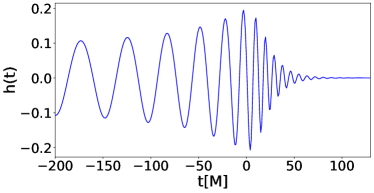
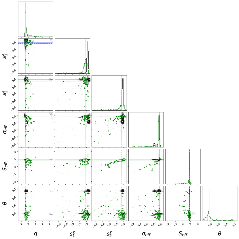
Figure 8: Probabilistic AI and Bayesian inference results, $q=1$ case. AI posterior distributions (in black), PyCBC Inference results (in green), and ground truth values (in blue) for an equal mass-ratio binary black hole merger. AI histograms show the distribution of $100,000$ samples drawn from the posterior.

                                                                         

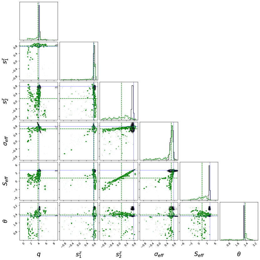
Figure 9: Probabilistic AI and Bayesian inference results, $q=4$, positive and aligned spin case. As Figure 8, but now for a binary with mass-ratio $q=4$ whose binary components are rapidly spinning.

                                                                         

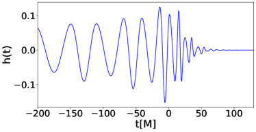
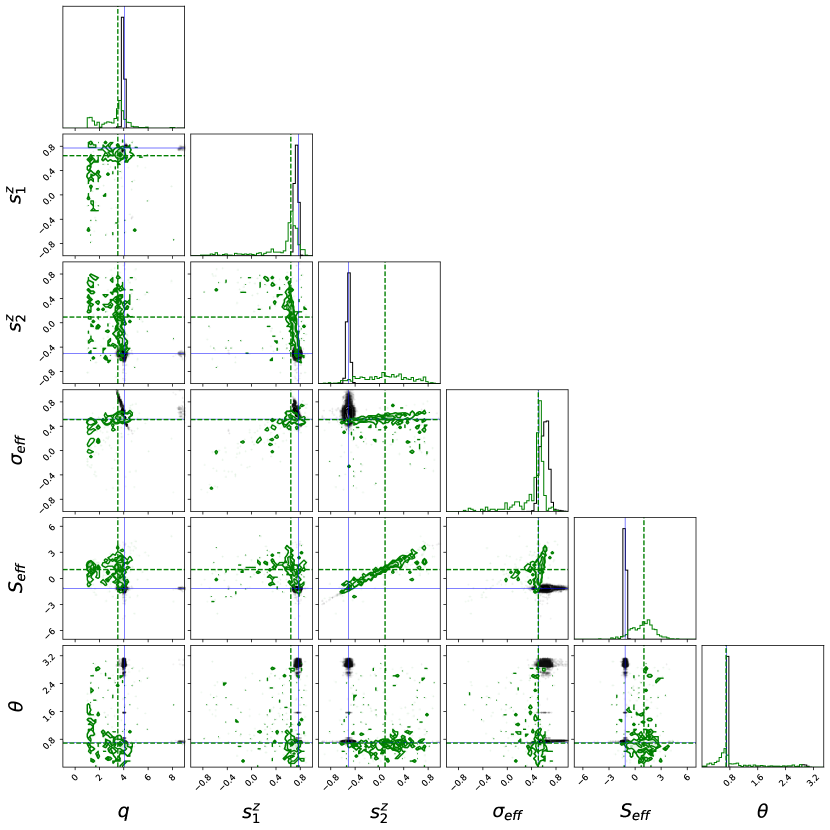
Figure 10: Probabilistic AI and Bayesian inference results, $q=4$, anti-aligned spin case. As Figure 9, but now the secondary is slowly rotating in the $-z$ direction.

                                                                         

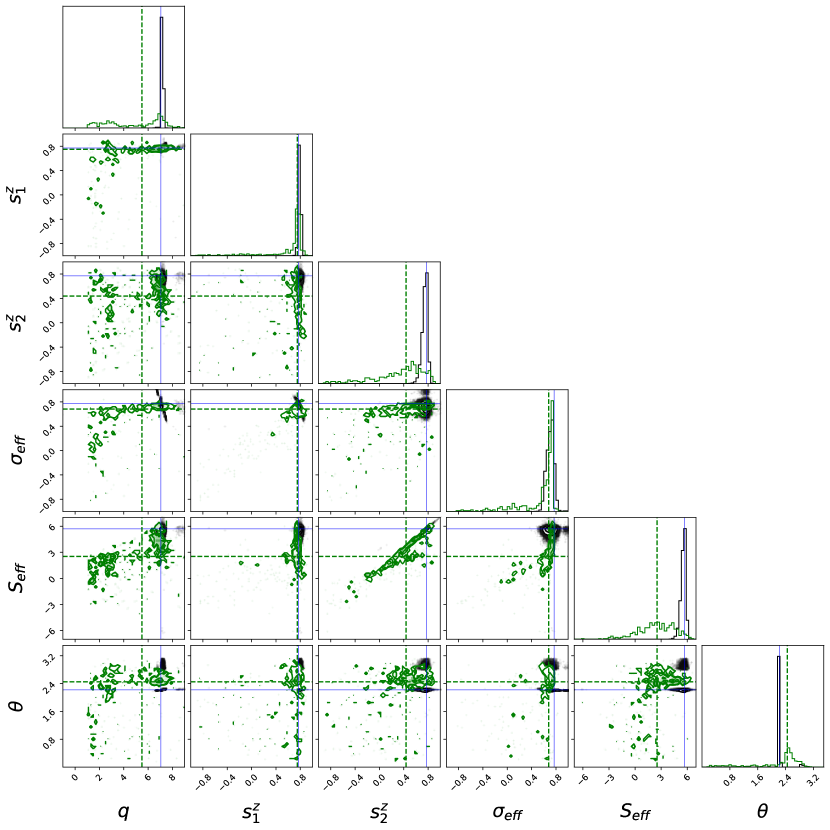
Figure 11: Probabilistic AI and Bayesian inference results, $q=7$, positive and aligned case. As Figure 8, but now for a binary with mass-ratio $q=7$ whose binary components are rapidly spinning.

                                                                         

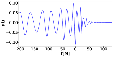
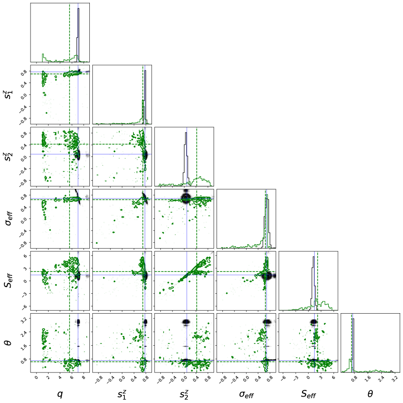
Figure 12: Probabilistic AI and Bayesian inference results, $q=7$, with primary rapidly rotating and secondary nearly spinless. As Figure 11, but now for a $q=7$ binary with a rapidly rotating primary and a nearly non-spinning secondary.

Benchmark results

These results provide evidence that AI surrogates are capable of learning and inferring the physics that describes quasi-circular, spinning, non-precessing, higher-order waveform modes of binary black hole mergers. In addition to these findings, we also provide results to compare the computational efficiency of AI and traditional Bayesian inference to produce Figures 8 to 12. In terms of computational performance we found that

• We produced AI results presented in these figures by drawing 100,000 samples from the posterior distribution using normalizing flow. This is done in less than a second using a single A100 NVIDIA GPU for all cases under consideration, i.e., irrespective of the properties of the binary black hole merger.

• For PyCBC Inference, we used 10 single-thread processes on an AMD EPYC 7352 with 24 physical cores to draw a similar amount of samples from the posterior distribution within

  1 hour 41 minutes for Figure 8

  3 hours 49 minutes for Figure 9

  4 hours 21 minutes for Figure 10

  6 hours 37 minutes for Figure 11

  2 hours 20 minutes for Figure 12

In summary, our probabilistic AI surrogates are between three to four orders of magnitude faster than traditional Bayesian inference methods. These results also indicate that we should clearly differentiate the physics we can infer from gravitational waves, and how the choice of signal processing tools will enhance or limit the science reach of our studies. For instance, it has been argued in the literature that it would be difficult to infer the spin of the secondary for asymmetric mass-ratio binaries, since the rotation of the lighter black hole has a marginal influence on the morphology of the waveform. What we are learning from this study is that we ought to tell apart the physics of the problem from the signal processing tools utilized to study the astrophysical properties of compact binaries, and for that matter for any system. It is true that traditional Bayesian inference is unable to provide informative constraints for the spin of the secondary, even for moderately asymmetric mass-ratio mergers, as we see in Figures 9 and 10; or for asymmetric mass-ratio systems, as we see in Figures 11 and 12. However, our probabilistic AI models do provide informative constraints for the spin of the primary and secondary for binaries with mass-ratios $1\leq q\leq 8$. This is because the subtle features and patterns that the spin of the secondary imprints in the waveform signal are identified and learned by AI, and this empowers us to infer these astrophysical parameters from complex signals that include higher-order waveform modes.

We also learn another piece of information from this analysis. As the broader community continues to develop AI-driven methodologies for accelerated inference, we should endeavor to develop novel AI tools, and to not limit the capabilities of these algorithms to simply accelerate parameter estimation analyses, providing nearly identical results to traditional Bayesian inference pipelines. Doing so will limit our ability to learn new insights from gravitational wave observations. As we have learned from this study, AI methods that are designed to mimic Bayesian pipelines will provide uninformative constraints on the spin distribution of compact binaries, in particular for the secondary, thereby limiting the knowledge or insights we could gain about the formation channels of these sources. Similarly, uninformative constraints for the inclination angle of these sources would have implications for gravitational wave cosmology.

This study has shown that in the case where we look at the signal manifold of higher-order waveform signals for black hole mergers, there is a wealth of astrophysical information we can extract from these signals using probabilistic AI methods. We have also learned that Bayesian approaches cannot capture features and patterns that enable the measurement of important astrophysical parameters, and that this is not a result of biases introduced by noise, since we are not considering the effect of noise at this stage. These signal processing limitations in parameter estimation are inherent to traditional Bayesian inference.

Another important result result of this paper is that we have designed a methodology to train AI models that adequately handle training datasets that include tens of millions of modeled waveforms, thereby paving the way to extend this analysis for the case in which these types of signals are contaminated with simulated and advanced LIGO noise. The methods introduced in this paper will enable us to quantify the biases introduced by noise in parameter estimation analyses, and how to handle them to extract informative AI-driven parameter estimation results using higher order gravitational wave modes.

4 Conclusions

We have developed scalable and computationally efficient methods to design AI models that are capable of characterizing the signal manifold of higher order wave modes of quasi-circular, spinning, non-precessing binary black hole mergers. Our approached enabled us to train several AI models using a dataset of over 14 million waveforms within 3.4 hours with 256 nodes, equivalent to 1,536 NVIDIA V100 GPUs, achieving optimal convergence and state-of-the-art regression results.

We have demonstrated that AI can abstract knowledge from time-series data that help constrain the physical parameters that determine the dynamical evolution of higher order modes of black hole mergers. In particular, we have presented evidence that AI provides deterministic and probabilistic predictions that tightly constrain the mass-ratio, individual spins, inclination angle, and effective spin parameters for a variety of astrophysical scenarios. We also found that deterministic and probabilistic AI predictions are consistent with each other, and in good accord with ground truth physical parameters.

We have also demonstrated that our AI surrogates outperform other machine learning methods (encompassing Gaussian regression, random forest, k-nearest neighbors, and linear regression), and PyCBC Inference both in terms of computational efficiency and accuracy. The results we have introduced in this article provide benchmarks for the expected performance of AI to estimate the astrophysical parameters of binary black hole mergers in the absence of noise. In future work, we will present studies for the impact of simulated and advanced LIGO noise to conduct informative AI-driven inference for high dimensional waveform manifolds.

5 Acknowledgements

A.K. and E.A.H. gratefully acknowledge National Science Foundation (NSF) awards OAC-1931561 and OAC-1934757, and the Innovative and Novel Computational Impact on Theory and Experiment project ‘Multi-Messenger Astrophysics at Extreme Scale in Summit’. P.K. acknowledges support of the Department of Atomic Energy, Government of India, under project no. RTI4001, and by the Ashok and Gita Vaish Early Career Faculty Fellowship at the International Centre for Theoretical Sciences. This material is based upon work supported by Laboratory Directed Research and Development (LDRD) funding from Argonne National Laboratory, provided by the Director, Office of Science, of the U.S. Department of Energy under Contract No. DE-AC02-06CH11357. This research used resources of the Argonne Leadership Computing Facility, which is a DOE Office of Science User Facility supported under Contract DE-AC02-06CH11357. This research used resources of the Oak Ridge Leadership Computing Facility, which is a DOE Office of Science User Facility supported under contract no. DE-AC05-00OR22725. This work utilized resources supported by the NSF’s Major Research Instrumentation program, the HAL cluster (grant no. OAC-1725729), as well as the University of Illinois at Urbana-Champaign. We thank NVIDIA for their continued support.

References

- [1] Y. LeCun, Y. Bengio, and G. Hinton, “Deep learning,” Nature, vol. 521, no. 7553, pp. 436–444, 2015.
- [2] A. Davies, P. Veličković, L. Buesing, S. Blackwell, D. Zheng, N. Tomašev, R. Tanburn, P. Battaglia, C. Blundell, A. Juhász, M. Lackenby, G. Williamson, D. Hassabis, and P. Kohli, “Advancing mathematics by guiding human intuition with ai,” Nature, vol. 600, pp. 70–74, 12 2021.
- [3] D. George and E. A. Huerta, “Deep neural networks to enable real-time multimessenger astrophysics,” Phys. Rev. D, vol. 97, p. 044039, Feb 2018.
- [4] D. George and E. Huerta, “Deep learning for real-time gravitational wave detection and parameter estimation: Results with advanced ligo data,” Physics Letters B, vol. 778, pp. 64 – 70, 2018.
- [5] E. A. Huerta, G. Allen, I. Andreoni, J. M. Antelis, E. Bachelet, G. B. Berriman, F. B. Bianco, R. Biswas, M. Carrasco Kind, K. Chard, M. Cho, P. S. Cowperthwaite, Z. B. Etienne, M. Fishbach, F. Forster, D. George, T. Gibbs, M. Graham, W. Gropp, R. Gruendl, A. Gupta, R. Haas, S. Habib, E. Jennings, M. W. G. Johnson, E. Katsavounidis, D. S. Katz, A. Khan, V. Kindratenko, W. T. C. Kramer, X. Liu, A. Mahabal, Z. Marka, K. McHenry, J. M. Miller, C. Moreno, M. S. Neubauer, S. Oberlin, A. R. Olivas, D. Petravick, A. Rebei, S. Rosofsky, M. Ruiz, A. Saxton, B. F. Schutz, A. Schwing, E. Seidel, S. L. Shapiro, H. Shen, Y. Shen, L. P. Singer, B. M. Sipocz, L. Sun, J. Towns, A. Tsokaros, W. Wei, J. Wells, T. J. Williams, J. Xiong, and Z. Zhao, “Enabling real-time multi-messenger astrophysics discoveries with deep learning,” Nature Reviews Physics, vol. 1, pp. 600–608, Oct. 2019.
- [6] E. A. Huerta and Z. Zhao, Advances in Machine and Deep Learning for Modeling and Real-Time Detection of Multi-messenger Sources, pp. 1–27. Singapore: Springer Singapore, 2020.
- [7] E. Cuoco, J. Powell, M. Cavaglià, K. Ackley, M. Bejger, C. Chatterjee, M. Coughlin, S. Coughlin, P. Easter, R. Essick, H. Gabbard, T. Gebhard, S. Ghosh, L. Haegel, A. Iess, D. Keitel, Z. Marka, S. Marka, F. Morawski, T. Nguyen, R. Ormiston, M. Puerrer, M. Razzano, K. Staats, G. Vajente, and D. Williams, “Enhancing Gravitational-Wave Science with Machine Learning,” Mach. Learn. Sci. Tech., vol. 2, no. 1, p. 011002, 2021.
- [8] H. Gabbard, M. Williams, F. Hayes, and C. Messenger, “Matching Matched Filtering with Deep Networks for Gravitational-Wave Astronomy,” Physical Review Letters, vol. 120, p. 141103, Apr. 2018.
- [9] V. Skliris, M. R. K. Norman, and P. J. Sutton, “Real-Time Detection of Unmodeled Gravitational-Wave Transients Using Convolutional Neural Networks,” arXiv e-prints, p. arXiv:2009.14611, Sept. 2020.
- [10] Y.-C. Lin and J.-H. P. Wu, “Detection of gravitational waves using bayesian neural networks,” Phys. Rev. D, vol. 103, p. 063034, Mar 2021.
- [11] H. Wang, S. Wu, Z. Cao, X. Liu, and J.-Y. Zhu, “Gravitational-wave signal recognition of LIGO data by deep learning,” Phys. Rev. D, vol. 101, no. 10, p. 104003, 2020.
- [12] X. Fan, J. Li, X. Li, Y. Zhong, and J. Cao, “Applying deep neural networks to the detection and space parameter estimation of compact binary coalescence with a network of gravitational wave detectors,” Sci. China Phys. Mech. Astron., vol. 62, no. 6, p. 969512, 2019.
- [13] X.-R. Li, G. Babu, W.-L. Yu, and X.-L. Fan, “Some optimizations on detecting gravitational wave using convolutional neural network,” Front. Phys. (Beijing), vol. 15, no. 5, p. 54501, 2020.
- [14] D. S. Deighan, S. E. Field, C. D. Capano, and G. Khanna, “Genetic-algorithm-optimized neural networks for gravitational wave classification,” arXiv e-prints, p. arXiv:2010.04340, Oct. 2020.
- [15] A. L. Miller et al., “How effective is machine learning to detect long transient gravitational waves from neutron stars in a real search?,” Phys. Rev. D, vol. 100, no. 6, p. 062005, 2019.
- [16] P. G. Krastev, “Real-Time Detection of Gravitational Waves from Binary Neutron Stars using Artificial Neural Networks,” Phys. Lett. B, vol. 803, p. 135330, 2020.
- [17] M. B. Schäfer, F. Ohme, and A. H. Nitz, “Detection of gravitational-wave signals from binary neutron star mergers using machine learning,” Phys. Rev. D , vol. 102, p. 063015, Sept. 2020.
- [18] C. Dreissigacker and R. Prix, “Deep-Learning Continuous Gravitational Waves: Multiple detectors and realistic noise,” Phys. Rev. D, vol. 102, no. 2, p. 022005, 2020.
- [19] A. Rebei, E. A. Huerta, S. Wang, S. Habib, R. Haas, D. Johnson, and D. George, “Fusing numerical relativity and deep learning to detect higher-order multipole waveforms from eccentric binary black hole mergers,” Phys. Rev. D , vol. 100, p. 044025, Aug 2019.
- [20] C. Dreissigacker, R. Sharma, C. Messenger, R. Zhao, and R. Prix, “Deep-Learning Continuous Gravitational Waves,” Phys. Rev. D, vol. 100, no. 4, p. 044009, 2019.
- [21] B. Beheshtipour and M. A. Papa, “Deep learning for clustering of continuous gravitational wave candidates,” Phys. Rev. D , vol. 101, p. 064009, Mar. 2020.
- [22] M. B. Schäfer and A. H. Nitz, “From one to many: A deep learning coincident gravitational-wave search,” Phys. Rev. D, vol. 105, no. 4, p. 043003, 2022.
- [23] M. B. Schäfer, O. Zelenka, A. H. Nitz, F. Ohme, and B. Brügmann, “Training strategies for deep learning gravitational-wave searches,” Phys. Rev. D, vol. 105, no. 4, p. 043002, 2022.
- [24] A. Gunny, D. Rankin, J. Krupa, M. Saleem, T. Nguyen, M. Coughlin, P. Harris, E. Katsavounidis, S. Timm, and B. Holzman, “Hardware-accelerated Inference for Real-Time Gravitational-Wave Astronomy,” Nature Astron., vol. 6, no. 5, pp. 529–536, 2022.
- [25] H. Shen, D. George, E. A. Huerta, and Z. Zhao, “Denoising gravitational waves with enhanced deep recurrent denoising auto-encoders,” in ICASSP 2019-2019 IEEE International Conference on Acoustics, Speech and Signal Processing (ICASSP), pp. 3237–3241, IEEE, 2019.
- [26] W. Wei and E. A. Huerta, “Gravitational wave denoising of binary black hole mergers with deep learning,” Physics Letters B, vol. 800, p. 135081, Jan. 2020.
- [27] R. Ormiston, T. Nguyen, M. Coughlin, R. X. Adhikari, and E. Katsavounidis, “Noise reduction in gravitational-wave data via deep learning,” Phys. Rev. Research, vol. 2, p. 033066, Jul 2020.
- [28] H. Shen, E. A. Huerta, E. O’Shea, P. Kumar, and Z. Zhao, “Statistically-informed deep learning for gravitational wave parameter estimation,” Machine Learning: Science and Technology, vol. 3, p. 015007, nov 2021.
- [29] H. Gabbard, C. Messenger, I. S. Heng, F. Tonolini, and R. Murray-Smith, “Bayesian parameter estimation using conditional variational autoencoders for gravitational-wave astronomy,” Nature Physics, vol. 18, pp. 112–117, Jan. 2022.
- [30] A. J. Chua and M. Vallisneri, “Learning Bayesian posteriors with neural networks for gravitational-wave inference,” Phys. Rev. Lett., vol. 124, no. 4, p. 041102, 2020.
- [31] S. R. Green, C. Simpson, and J. Gair, “Gravitational-wave parameter estimation with autoregressive neural network flows,” Phys. Rev. D, vol. 102, p. 104057, Nov 2020.
- [32] S. R. Green and J. Gair, “Complete parameter inference for gw150914 using deep learning,” Machine Learning: Science and Technology, vol. 2, p. 03LT01, June 2020.
- [33] M. Dax, S. R. Green, J. Gair, J. H. Macke, A. Buonanno, and B. Schölkopf, “Real-time gravitational-wave science with neural posterior estimation,” arXiv e-prints, p. arXiv:2106.12594, June 2021.
- [34] M. Dax, S. R. Green, J. Gair, M. Deistler, B. Schölkopf, and J. H. Macke, “Group equivariant neural posterior estimation,” arXiv e-prints, p. arXiv:2111.13139, Nov. 2021.
- [35] S. Khan and R. Green, “Gravitational-wave surrogate models powered by artificial neural networks,” Phys. Rev. D, vol. 103, no. 6, p. 064015, 2021.
- [36] A. J. K. Chua, C. R. Galley, and M. Vallisneri, “Reduced-order modeling with artificial neurons for gravitational-wave inference,” Phys. Rev. Lett., vol. 122, p. 211101, May 2019.
- [37] J. Lee, S. H. Oh, K. Kim, G. Cho, J. J. Oh, E. J. Son, and H. M. Lee, “Deep learning model on gravitational waveforms in merging and ringdown phases of binary black hole coalescences,” Phys. Rev. D , vol. 103, p. 123023, June 2021.
- [38] A. Khan, E. A. Huerta, and H. Zheng, “Interpretable AI forecasting for numerical relativity waveforms of quasicircular, spinning, nonprecessing binary black hole mergers,” Phys. Rev. D , vol. 105, p. 024024, Jan. 2022.
- [39] W. Wei, E. A. Huerta, M. Yun, N. Loutrel, M. A. Shaikh, P. Kumar, R. Haas, and V. Kindratenko, “Deep Learning with Quantized Neural Networks for Gravitational-wave Forecasting of Eccentric Compact Binary Coalescence,” Astrophys. J., vol. 919, p. 82, Oct. 2021.
- [40] W. Wei and E. A. Huerta, “Deep learning for gravitational wave forecasting of neutron star mergers,” Phys. Lett. B, vol. 816, p. 136185, 2021.
- [41] H. Yu, R. X. Adhikari, R. Magee, S. Sachdev, and Y. Chen, “Early warning of coalescing neutron-star and neutron-star-black-hole binaries from the nonstationary noise background using neural networks,” Phys. Rev. D , vol. 104, p. 062004, Sept. 2021.
- [42] S. G. Rosofsky and E. A. Huerta, “Artificial neural network subgrid models of 2D compressible magnetohydrodynamic turbulence,” Phys. Rev. D , vol. 101, p. 084024, Apr. 2020.
- [43] P. I. Karpov, C. Huang, I. Sitdikov, C. L. Fryer, S. Woosley, and G. Pilania, “Physics-Informed Machine Learning for Modeling Turbulence in Supernovae,” arXiv e-prints, p. arXiv:2205.08663, May 2022.
- [44] S. G. Rosofsky and E. A. Huerta, “Applications of physics informed neural operators,” arXiv e-prints, p. arXiv:2203.12634, Mar. 2022.
- [45] E. A. Huerta, A. Khan, X. Huang, M. Tian, M. Levental, R. Chard, W. Wei, M. Heflin, D. S. Katz, V. Kindratenko, D. Mu, B. Blaiszik, and I. Foster, “Accelerated, scalable and reproducible AI-driven gravitational wave detection,” Nature Astronomy, vol. 5, pp. 1062–1068, July 2021.
- [46] P. Chaturvedi, A. Khan, M. Tian, E. A. Huerta, and H. Zheng, “Inference-Optimized AI and High Performance Computing for Gravitational Wave Detection at Scale,” Front. Artif. Intell., vol. 5, p. 828672, 2022.
- [47] E. A. Huerta, A. Khan, E. Davis, C. Bushell, W. D. Gropp, D. S. Katz, V. Kindratenko, S. Koric, W. T. C. Kramer, B. McGinty, K. McHenry, and A. Saxton, “Convergence of Artificial Intelligence and High Performance Computing on NSF-supported Cyberinfrastructure,” Journal of Big Data, vol. 7, no. 1, p. 88, 2020.
- [48] A. Khan, E. A. Huerta, and A. Das, “Physics-inspired deep learning to characterize the signal manifold of quasi-circular, spinning, non-precessing binary black hole mergers,” Physics Letters B, vol. 808, p. 135628, Sept. 2020.
- [49] V. Varma, S. E. Field, M. A. Scheel, J. Blackman, L. E. Kidder, and H. P. Pfeiffer, “Surrogate model of hybridized numerical relativity binary black hole waveforms,” Phys. Rev. D, vol. 99, p. 064045, Mar 2019.
- [50] E. T. Newman and R. Penrose, “Note on the bondi-metzner-sachs group,” Journal of Mathematical Physics, vol. 7, no. 5, pp. 863–870, 1966.
- [51] J. N. Goldberg, A. J. Macfarlane, E. T. Newman, F. Rohrlich, and E. C. G. Sudarshan, “Spin-s Spherical Harmonics and h,” Journal of Mathematical Physics, vol. 8, pp. 2155–2161, Nov. 1967.
- [52] “Gravitational Radiation from Post-Newtonian Sources and Inspiralling Compact Binaries,” Living Reviews in Relativity, vol. 17, p. 2, Dec. 2014.
- [53] A. van den Oord, S. Dieleman, H. Zen, K. Simonyan, O. Vinyals, A. Graves, N. Kalchbrenner, A. Senior, and K. Kavukcuoglu, “Wavenet: A generative model for raw audio,” 2016.
- [54] Y. You, J. Li, S. Reddi, J. Hseu, S. Kumar, S. Bhojanapalli, X. Song, J. Demmel, K. Keutzer, and C.-J. Hsieh, “Large batch optimization for deep learning: Training bert in 76 minutes,” 2019.
- [55] S. R. Green and J. Gair, “Complete parameter inference for gw150914 using deep learning,” Machine Learning: Science and Technology, vol. 2, no. 3, p. 03LT01, 2021.
- [56] C. Durkan, A. Bekasov, I. Murray, and G. Papamakarios, “nflows: normalizing flows in PyTorch,” Nov. 2020.
- [57] C. Durkan, A. Bekasov, I. Murray, and G. Papamakarios, “Neural spline flows,” Advances in Neural Information Processing Systems, vol. 32, pp. 7511–7522, 2019.
- [58] C. Biwer, C. D. Capano, S. De, M. Cabero, D. A. Brown, A. H. Nitz, and V. Raymond, “PyCBC Inference: A Python-based parameter estimation toolkit for compact binary coalescence signals,” Publ. Astron. Soc. Pac., vol. 131, no. 996, p. 024503, 2019.
- [59] L. Barsotti, S. Gras, M. Evans, and P. Fritschel, “Advanced LIGO anticipated sensitivity curves,” 2018. https://dcc.ligo.org/LIGO-T1800044/public.