Non-linear shrinkage of the price return covariance matrix is far from optimal for portfolio optimisation

Abstract

Portfolio optimization requires sophisticated covariance estimators that are able to filter out estimation noise. Non-linear shrinkage is a popular estimator based on how the Oracle eigenvalues can be computed using only data from the calibration window. Contrary to common belief, NLS is not optimal for portfolio optimization because it does not minimize the right cost function when the asset dependence structure is non-stationary. We instead derive the optimal target. Using historical data, we quantify by how much NLS can be improved. Our findings reopen the question of how to build the covariance matrix estimator for portfolio optimization in realistic conditions.

1 Introduction

Covariance filtering is essential in multivariate Finance [1] and in all scientific fields (see [2] for a recent review). A very popular family of estimators filters the covariance matrix by only changing its eigenvalues while keeping its eigenvectors untouched. They are known as Rotationally Invariant Estimators (RIEs). The best known RIE is linear shrinkage [3]. More recently, several methods of non-linear shrinkage (NLS) have been introduced [4, 5, 6, 7]. NLS asymptotically converges to the Oracle estimator, which minimizes the Frobenius (element-wise square) distance between the filtered and the true population covariance matrix. The asymptotic limit corresponds to infinitely large data matrices at fixed aspect ratio (the number of lines divided by the number of columns). Two important conditions must be met to achieve this convergence: the dependence structure between the time series must be constant, and the price return distribution must not be too heavy-tailed [4, 5, 6, 7].

Because NLS is provably a best estimator is some sense, it is also widely used for portfolio optimization ([8, 9, 10, 11, 12, 13, 14] among hundreds of references), including in the much cited the state-of-the-art combination of dynamic conditional covariance and NLS [15, 16]. This results from the implicit belief that Frobenius-optimal eigenvalues are also optimal for portfolio optimization, or equivalently that the Oracle eigenvalues inevitably provide the best (or almost the best) eigenvalues for portfolio optimization. There is however no proof that it is actually the case.

Our main hypothesis is that the covariance matrix eigenvalues that are best for global minimum variance minimization do not coincide with the Oracle eigenvalues and thus that non-linear shrinkage is not optimal in general. A conceptually simple way to demonstrate this hypothesis is to compute the RIE eigenvalues that do yield the optimal Global Minimum Variance portfolio and show that this RIE outperforms the Oracle. Such an estimator is obtained solving a quadratic programming problem, which admits an optimal solution different from the Oracle.

We investigate with real financial data where this discrepancy comes from and reversely in which conditions the NLS is a good approximation to the optimal eigenvalues. We found that only when both calibration and test windows are very large with respect to the number of stocks and when the covariance coefficients between calibration and test differs only due to sample size noise (in other words, both sample covariance matrices have the same expected covariance matrix), then the two estimators share similar performances.

2 Problem Statement

Consider $n$ price return time series split into a calibration time window of length $\delta_{in}$ and a test time windows of length $\delta_{out}$, and let us denote the in-sample (empirical) covariance matrix by ${\bf\Sigma}^{\textrm{in}}\in\mathbb{R}^{n\times n}$ and the out-of-sample (realized) covariance matrix by ${\bf\Sigma}^{\textrm{out}}\in\mathbb{R}^{n\times n}$ respectively. According to the spectral theorem, the in-sample covariance matrix can be decomposed into a sum of terms involving its eigenvalues $\mathbf{\lambda}=(\lambda_{k})\in\mathbb{R}^{n}$ and their associated eigenvectors components $v_{i}=(v_{ik})\in\mathbb{R}^{n}$ as

$$\Sigma_{ij}^{\textrm{in}}=\sum_{k=1}^{n}\lambda_{k}^{\textrm{in}}v_{ik}^{\textrm{in}}v_{jk}^{\textrm{in}}.$$ (1)

An RIE estimator $\Xi({\bf\lambda}^{*})$ uses filtered eigenvalues, which yields the spectral decomposition

$$\Xi({\bf\lambda}^{*})_{ij}=\sum_{k=1}^{n}\lambda_{k}^{*}v_{ik}^{\textrm{in}}v_{jk}^{\textrm{in}},$$ (2)

where $\bf{\lambda}^{*}$ are a set of filtered eigenvalues obtained with some procedure and ${\bf v}^{\textrm{in}}$ are still the eigenvectors of ${\bf\Sigma}^{\textrm{in}}$.

We aim to compare the filtered eigenvalues from NLS and from the ones that are actually optimal for portfolio optimization.

2.1 Oracle Eigenvalues

The Oracle eigenvalues are obtained from the out-of-sample covariance matrix from

$$\lambda^{\textrm{Oracle}}_{k}=\sum_{i=1}^{n}\sum_{j=1}^{n}v_{ik}^{\textrm{in}}\Sigma_{ij}^{\textrm{out}}v_{jk}^{\textrm{in}},$$ (3)

where $v^{\textrm{in}}$ are the in-sample eigenvectors.

Such an eigenvalue correction provably produces an estimator that minimizes the Frobenius norm [4, 7]

$$||\Xi(\lambda^{\textrm{Oracle}})-\Sigma^{\textrm{out}}||_{F}=\sum_{i=1}^{n}\sum_{j=1}^{n}\left[\Xi(\lambda^{\textrm{Oracle}})_{ij}-\Sigma^{\textrm{out}}_{ij}\right]^{2}.$$ (4)

2.2 Optimal RIEs for GMV Portfolios

The simplest portfolio optimization problem (and the most relevant one to assess covariance filtering methods) is Global Minimum Variance (GMV) portfolios. We denote the fraction of capital assigned to each possible asset $i=1,\cdots,n$ by $\mathbf{w}\in\mathbb{R}^{n}$. GMV portfolios aim to minimize the realized portfolio variance $\Sigma^{\textrm{out}}$ at fixed net leverage $\sum_{i}w_{i}=1$. Mathematically, the problem can be written as the function of the weights as

$$\min_{w}\sum_{i=1}^{n}\sum_{j=1}^{n}w_{i}\Sigma_{ij}^{\textrm{out}}w_{j}~{}~{}~{}\textrm{with }\sum_{k=1}^{N}w_{k}=1.$$ (5)

This problem is readily solved if the future is known: the optimal GMV weights are given by

$$\mathbf{w}_{\textrm{opt}}=\frac{(\Sigma^{\textrm{out}})^{-1}\mathbf{e}}{\mathbf{e}^{\prime}(\Sigma^{\textrm{out}})^{-1}\mathbf{e}},$$ (6)

where $\mathbf{e}={1,\cdots,1}$ is a $n$-dimensional vector of ones.

The main contribution of this paper is to show how not optimal NLS is for GMV portfolio optimization in a practical context. To this end, we compute the GMV-optimal RIE, which constrains the weights $\mathbf{w}$ to be written as a function of $\Xi(\mathbf{\lambda}^{*})$ instead of $\Sigma^{\textrm{out}}$, the optimization variables being $\Xi$’s eigenvalues. The optimal weights are now

$$w_{k}=\frac{\sum_{j=1}^{n}\Xi_{kj}^{-1}}{\sum_{i=1}^{n}\sum_{j=1}^{n}\Xi_{ij}^{-1}},$$ (7)

where ${\bf\Xi}^{-1}$ is the inverse covariance matrix RIE whose spectral decomposition is

$$\Xi_{ij}^{-1}=\sum_{k=1}^{n}\frac{1}{\lambda_{k}^{*}}v_{ik}^{\textrm{in}}v_{jk}^{\textrm{in}}.$$ (8)

It is important to point out that the denominator of 7 is a normalization factor which ensures that the sum of the weights equals one. Equation 7 is thus equivalent to

$$\begin{cases}w_{k}=\sum_{j=1}^{n}\Xi_{kj}^{-1};&k=1,\cdots,n\\ \sum_{k=1}^{n}w_{k}=1.\end{cases}$$ (9)

Another important point is that the optimal GMV portfolio obtained from 9 and 8 does not depend on the scale of the eigenvalues $\lambda_{k}^{*}$ (or, equivalently, the average volatility). Thus, the only constraints we must impose on the eigenvalues is their non-negativity

$$\zeta_{k}:=\frac{1}{\lambda_{k}^{*}}\geq 0;\,\,\,\mbox{for}\,\,\,k=1,\cdots,n.$$ (10)

Finally, the full QP problem is expressed as

$$\begin{array}[]{ll@{}ll}\min_{{\bf w,\Xi^{-}1,\zeta}}&\sum_{i=1}^{n}w_{i}\Sigma^{\textrm{out}}_{ij}w_{j}&\\ \text{subject to}&w_{k}=\sum_{j=1}^{n}\Xi_{kj}^{-1};&k=1,\cdots,n\\ &\sum_{k=1}^{n}w_{k}=1\\ &\Xi_{ij}^{-1}=\sum_{k=1}^{n}\zeta_{k}v_{ik}^{\textrm{in}}v_{jk}^{\textrm{in}};&i,j=1,\cdots,n\\ &\zeta_{k}\geq 0;&k=1,\cdots,n.\end{array}$$ (11)

Eq. 11 defines a convex Quadratic Programming problem, which can be solved by numerical methods. In this QP problem formulation the variables ${\bf w}$ and ${\bf\Xi}^{-1}$ are slack variables that will be identified by the optimization algorithm. In total, the QP has $n(n+5)/2$ variables: $n$ for ${\bf w}$, $n(n+1)/2$ for ${\bf\Xi}^{-1}$, as the inverse covariance is symmetric, and $n$ for ${\bf\zeta}$ which are of interest here. The number of constraints are $(n^{2}+5n+2)/2$. The resulting optimal $\zeta_{k}$ can be then normalized to have a set of eigenvalues whose sum equals expected volatility.

The procedure described above does not guarantee an ordered sequence of optimal eigenvalues. Let us therefore add $n-1$ ordering constraints to Eq. 11, which yields

$$\begin{array}[]{ll@{}ll}\min_{{\bf w,\Xi^{-1},\zeta}}&\sum_{i=1}^{n}w_{i}\Sigma^{\textrm{out}}_{ij}w_{j}&\\ \text{subject to}&w_{k}=\sum_{j=1}^{n}\Xi_{kj}^{-1};&k=1,\cdots,n\\ &\sum_{k=1}^{n}w_{k}=1\\ &\Xi_{ij}^{-1}=\sum_{k=1}^{n}\zeta_{k}v_{ik}^{\textrm{in}}v_{jk}^{\textrm{in}};{}&i,j=1,\cdots,n\\ &\zeta_{k}\geq 0;&k=1,\cdots,n\\ &\zeta_{k}\geq\zeta_{k-1};&k=2,\cdots,n.\end{array}$$ (12)

These constraints necessarily imply a less optimal solution with respect to the unsorted case. A Python implementation of both QP problems is available from [17].

3 Results: real Global Minimum Variance portfolios

We apply both estimators to a data set of adjusted daily returns of the most capitalized US equities spanning the 1995-2017 period.

The experiments are carried out in the following way. We randomly select two contiguous time intervals $[t-\delta_{\textrm{in}},t[$ and $[t,t+\delta_{\textrm{out}}[$ from the whole period, remove all the stocks which have more than $20\%$ of missing values or zero returns, and discard any two stocks with an in-sample correlation larger than $0.95$. From the remaining assets, we randomly select $n=50$ stocks and we compute $\Sigma^{\textrm{in}}$ and $\Sigma^{\textrm{out}}$ from the two intervals respectively.

From the eigenvector basis of $\Sigma^{\textrm{in}}$ and $\Sigma^{\textrm{out}}$ we compute the optimal eigenvalues (Eqs  (11)), the sorted optimal eigenvalue and the Oracle ones (Eqs (12)) and the Oracle eigenvalues, which optimize the Frobenius norm. We stress that NLS aims to approximate the Oracle eigenvalues, thus produces slightly worse results [18]. For that reason, we only include the Oracle eigenvalues in our study. Finally, we compute the out-of-sample (realized volatility) of GMV portfolios for each RIE.

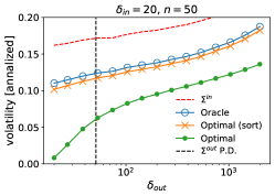
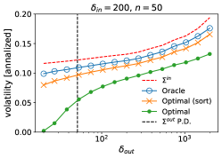
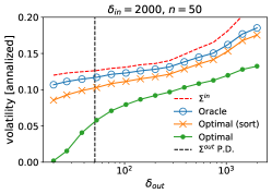
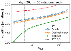
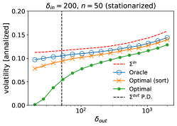
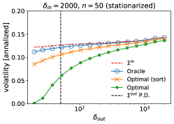
Figure 1: Realized volatility as a function of the out-of-sample period length. The upper panels display results from the original data, while the lower ones use stationarized data. The vertical black dotted lines refer to the transition point $n=\delta_{\textrm{out}}$ to a positive-defined out-of-sample covariance matrix. Matrix inversion of $\Sigma^{\textrm{in}}$ for $\delta_{\textrm{out}}<n+1$ is obtained with a pseudo-inverse [19]. Averages over 10,000 portfolios of $n=50$ random assets in random periods from daily data (large capitalization US equities).

In the upper panels of Fig. 1, we show the average annualized volatility over 10,000 portfolios with randomly chosen assets at random times. The performance ranking is always the same one: applying Oracle correction is always better than using only the past ($\Sigma^{\textrm{in}}$, and the weights from the QP problem are always better than the Oracle RIE.

One notices a large gap between the Optimal and the Optimal sorted weights; when $\delta_{\textrm{out}}<n+1$, this gap comes from the fact that when $\delta_{\textrm{out}}<n+1$, the out-of-sample covariance matrix is not positively-defined. This means that there are $d=n+1-\delta_{\textrm{out}}$ null eigenvalues which imply an eigenspace of dimension $d$ from which every portfolio will have null variance. This is a purely mechanical effect that cannot be exploited from in-sample data only. This gap disappears when the monotonicity of the filtered eigenvalues is imposed. Interestingly, when $\delta_{\textrm{out}}>n+1$ the difference of performance between all the methods remains approximately constant until $\delta_{\textrm{out}}$ reaches very large values (1000 days, i.e., about 4 years of data). The phenomenon occurs when the in-sample window size $\delta_{\textrm{in}}$ increases from $200$ to $2000$. This effect comes from the non-stationarity of the dependence structure in the financial data we use. As a consequence, very large calibration or test periods produce out-of-date eigenvector bases.

To confirm this hypothesis, we stationarize the in-sample and out-of-sample time-series. The idea is simply to shuffle the in-sample and out-of-sample days of each subperiod $[t-\delta_{\textrm{in}},t+\delta_{\textrm{out}}[$, in such a way that both the in-sample and out-of-sample holds a similar proportion of past and future days, which yields the same expected covariance matrix in both periods. In the lower panels of Fig. 1 we show that increasing both $\delta_{\textrm{in}}$ and $\delta_{\textrm{out}}$ on two stationarized time-series reduces substantially the bias. This comes from the fact that in these conditions, the in-sample and out-of-sample eigenvector bases tend to be very similar. If either of the two time-window lengths are reduced, the similarity between the two eigenvector bases decreases.

4 Conclusion

Covariance filtering for portfolio optimization, while having progressed much in the last decades, still needs fundamental improvements. The problem lies in the nonstationary nature of dependence in financial markets, which conflicts with one of the main assumptions of the optimal stationary RIE, and which implies that the Frobenius distance is not the right cost function for the optimal RIE in a non-stationary world. The correct optimal RIE, derived in this work, currently does not have any asymptotical estimator that use only in-sample data, and thus, finding the optimal covariance cleaning scheme for equity markets is still an open question.

Any improvement will mechanically improve on the state-of-the art DCC+NLS scheme [15]. The simplest route is to keep improving RIEs for which many exact asymptotic results are known [2]. For example, we recently showed that a long-term average approach of the Oracle eigenvalues outperforms the Oracle eigenvalues in systems with nonstationary dependencies such as US and Hong Kong equity markets [18].

We finally note that a RIE does not filter the noise in the eigenvectors which contain useful additional but noisy structures. A way to filter the latter is provided for example by ansätze such as hierarchical clustering [20] or probabilistic hierarchical clustering [21, 22], which outperform the optimal stationary RIE for GMV portfolios when $\delta_{\textrm{in}}<2n$ and DCC+NLS when the asset universe keeps changing, as it is the case in real life. An alternative route is to train a deep neural network to learn to predict both the eigenvalues and the eigenvectors.

Funding

This publication stems from a partnership between CentraleSupélec and BNP Paribas.

References

- [1] Richard O Michaud. The Markowitz optimization enigma: Is “optimized ” optimal? Financial Analysts Journal, 45(1):31–42, 1989.
- [2] Joël Bun, Jean-Philippe Bouchaud, and Marc Potters. Cleaning large correlation matrices: tools from random matrix theory. Physics Reports, 666:1–109, 2017.
- [3] Olivier Ledoit and Michael Wolf. A well-conditioned estimator for large-dimensional covariance matrices. Journal of multivariate analysis, 88(2):365–411, 2004.
- [4] Olivier Ledoit and Sandrine Péché. Eigenvectors of some large sample covariance matrix ensembles. Probability Theory and Related Fields, 151(1):233–264, 2011.
- [5] Olivier Ledoit, Michael Wolf, et al. Nonlinear shrinkage estimation of large-dimensional covariance matrices. The Annals of Statistics, 40(2):1024–1060, 2012.
- [6] Daniel Bartz. Cross-validation based nonlinear shrinkage. arXiv preprint arXiv:1611.00798, 2016.
- [7] Joël Bun, Romain Allez, Jean-Philippe Bouchaud, and Marc Potters. Rotational invariant estimator for general noisy matrices. IEEE Transactions on Information Theory, 62(12):7475–7490, 2016.
- [8] Taras Bodnar, Nestor Parolya, and Wolfgang Schmid. Estimation of the global minimum variance portfolio in high dimensions. European Journal of Operational Research, 266(1):371–390, 2018.
- [9] Yi Ding, Yingying Li, and Xinghua Zheng. High dimensional minimum variance portfolio estimation under statistical factor models. Journal of Econometrics, 222(1, Part B):502–515, 2021. Annals Issue:Financial Econometrics in the Age of the Digital Economy.
- [10] Francisco Rubio, Xavier Mestre, and Daniel P Palomar. Performance analysis and optimal selection of large minimum variance portfolios under estimation risk. IEEE Journal of Selected Topics in Signal Processing, 6(4):337–350, 2012.
- [11] Liusha Yang, Romain Couillet, and Matthew R McKay. A robust statistics approach to minimum variance portfolio optimization. IEEE Transactions on Signal Processing, 63(24):6684–6697, 2015.
- [12] Liusha Yang, Romain Couillet, and Matthew R McKay. Minimum variance portfolio optimization with robust shrinkage covariance estimation. In 2014 48th Asilomar Conference on Signals, Systems and Computers, pages 1326–1330. IEEE, 2014.
- [13] Ruili Sun, Tiefeng Ma, Shuangzhe Liu, and Milind Sathye. Improved covariance matrix estimation for portfolio risk measurement: A review. Journal of Risk and Financial Management, 12(1), 2019.
- [14] Zhao Zhao, Olivier Ledoit, and Hui Jiang. Risk reduction and efficiency increase in large portfolios: Gross-exposure constraints and shrinkage of the covariance matrix. Journal of Financial Econometrics, 2021.
- [15] Robert F. Engle, Olivier Ledoit, and Michael Wolf. Large dynamic covariance matrices. Journal of Business & Economic Statistics, 37(2):363–375, 2019.
- [16] Gianluca De Nard, Robert F Engle, Olivier Ledoit, and Michael Wolf. Large dynamic covariance matrices: Enhancements based on intraday data. Journal of Banking & Finance, 138:106426, 2022.
- [17] Christian Bongiorno. Optimal RIE, 2021. python3.5 package version 1.0.
- [18] Christian Bongiorno, Damien Challet, and Grégoire Loeper. Cleaning the covariance matrix of strongly nonstationary systems with time-independent eigenvalues. arXiv preprint arXiv:2111.13109, 2021.
- [19] Ester Pantaleo, Michele Tumminello, Fabrizio Lillo, and Rosario N Mantegna. When do improved covariance matrix estimators enhance portfolio optimization? an empirical comparative study of nine estimators. Quantitative Finance, 11(7):1067–1080, 2011.
- [20] Michele Tumminello, Fabrizio Lillo, and Rosario N Mantegna. Hierarchically nested factor model from multivariate data. EPL (Europhysics Letters), 78(3):30006, 2007.
- [21] Christian Bongiorno and Damien Challet. Covariance matrix filtering with bootstrapped hierarchies. PloS one, 16(1):e0245092, 2021.
- [22] Christian Bongiorno and Damien Challet. Reactive global minimum variance portfolios with bahc covariance cleaning. arXiv preprint arXiv:2005.08703, 2020.