The multirank likelihood for semiparametric canonical correlation analysis

Abstract

Many analyses of multivariate data are focused on evaluating the dependence between two sets of variables, rather than the dependence among individual variables within each set. Canonical correlation analysis (CCA) is a classical data analysis technique that estimates parameters describing the dependence between such sets. However, inference procedures based on traditional CCA rely on the assumption that all variables are jointly normally distributed. We present a semiparametric approach to CCA in which the multivariate margins of each variable set may be arbitrary, but the dependence between variable sets is described by a parametric model that provides low-dimensional summaries of dependence. While maximum likelihood estimation in the proposed model is intractable, we develop a novel MCMC algorithm called cyclically monotone Monte Carlo (CMMC) that provides estimates and confidence regions for the between-set dependence parameters. This algorithm is based on a multirank likelihood function, which uses only part of the information in the observed data in exchange for being free of assumptions about the multivariate margins. We apply the proposed inference procedure to Brazilian climate data and monthly stock returns from the materials and communications market sectors.

Keywords: Multivariate Analysis, Optimal Transport, Gaussian Copula, Bayesian Methods

1 Introduction

Scientific studies often involve the collection of multivariate data with complex interdependencies. In some cases, a study will be concerned with the pairwise dependence between individual variables. In other cases, however, the dependence of interest is between non-overlapping sets of variables. For instance, when analyzing financial data, it may be of interest to characterize the association between market sectors without regards to the dependence among stocks within a market sector. Other examples are encountered in biological studies concerning the relationship between diet and the human microbiome (Chen et al.,, 2013), psychological studies comparing attachment types to personality disorders (Sherry and Henson,, 2005), and neuroscience studies comparing brain imaging results to non-imaging measurements (see e.g. Winkler et al., (2020) for a survey).

One approach to characterizing the association between sets of variables is to conduct hypothesis tests for independence. Classical methods using Wilks’ $\Lambda$ statistic (Mardia et al.,, 1979), as well as modern methods using the distance covariance (Bakirov et al.,, 2006), and the Ball covariance (Pan et al.,, 2020) are available for this purpose. While each of these tests relies on some assumptions about the multivariate marginal distributions of the variable sets, recently Shi et al., (2020) and Deb and Sen, (2021) have proposed tests for independence that allow the marginal distributions of the variable sets to be arbitrary. In analogy to tests for independence based on univariate ranks, these tests are based on the multivariate ranks introduced by Chernozhukov et al., (2017).

The multivariate ranks described by these authors are appealing because test statistics based on these ranks yield approximate or exact null distributions that do not assume anything about the multivariate distributions of the variable sets. However, model-based approaches to the analysis of multivariate data have some advantages compared to such non-parametric approaches. For example, some models have parameters that provide low-dimensional summaries of the association between the variable sets, which may be scientifically interpretable. Canonical correlation analysis (CCA) is a classical data analysis technique that estimates such parameters. First described by Hotelling, (1936), CCA can be motivated from several perspectives, including invariance with respect to transformations under the general linear group (Eaton,, 1983), estimation in a latent factor model (Bach and Jordan,, 2005), and statistical whitening (Jendoubi and Strimmer,, 2019). Given random vectors $\boldsymbol{y}_{1},\boldsymbol{y}_{2}$ taking values in $\mathbb{R}^{p_{1}},\mathbb{R}^{p_{2}}$, CCA identifies a pair of linear transformations $\boldsymbol{B}_{1},\boldsymbol{B}_{2}$ such that the canonical variables $\boldsymbol{x}_{1}=\boldsymbol{B}^{\top}_{1}\boldsymbol{y}_{1}$ and $\boldsymbol{x}_{2}=\boldsymbol{B}^{\top}_{2}\boldsymbol{y}_{2}$ satisfy

$$\mathrm{Var}(\boldsymbol{x}_{1})={\bf I}_{p_{1}},~{}\mathrm{Var}(\boldsymbol{x}_{2})={\bf I}_{p_{2}},~{}\mathrm{Cov}(\boldsymbol{x}_{1},\boldsymbol{x}_{2})=\boldsymbol{\Lambda},$$

where $\boldsymbol{\Lambda}$ is a diagonal matrix with ordered diagonal entries $1>\lambda_{1}\geq\dots\geq\lambda_{d}\geq 0$, which are known as the canonical correlations. The ordering of the canonical correlations implies, for example, that the correlation of the first element of $\boldsymbol{x}_{1}$ with that of $\boldsymbol{x}_{2}$ is the largest among correlations between linear combinations of $\boldsymbol{y}_{1}$ with those of $\boldsymbol{y}_{2}$. Because they are a function of the original variables, the canonical variables may be useful in exploratory analyses where the goal is to understand which of the original variables is contributing to the association between variable sets. Additionally, the canonical correlations might be helpful in determining the effective dimensionality of the between-set association. However, estimation and uncertainty quantification for the parameters of CCA is challenging without the restrictive assumption that the variables from each set are jointly normally distributed.

In this article, we develop a semiparametric approach to CCA, which preserves the parametric model for between-set dependence, but allows the multivariate margins of each variable set to be arbitrary. Our model extends existing proposals for semiparametric CCA (Zoh et al.,, 2016; Agniel and Cai,, 2017; Yoon et al.,, 2020), which assume that the multivariate marginal distributions of the variable sets can be described by a Gaussian copula. In fact, our model may be seen as a generalization of the Gaussian copula model to vector-valued margins, much like the vector copula introduced by Fan and Henry, (2020). Unlike these authors, however, we present an inference strategy that allows for estimation of and uncertainty quantification for parameters describing the association between variable sets, even when the transformations parameterizing the multivariate margins are unknown. Our inference strategy is based on a multirank likelihood, which uses only part of the information in the observed data in exchange for being free of assumptions about the multivariate margins. While maximum likelihood estimation with the multirank likelihood is intractable, we show that Bayesian estimation of the between-set dependence parameters can be achieved with a novel Metropolis-Hastings algorithm called cyclically monotone Monte Carlo (CMMC).

In the first part of Section 2 of this article, we describe a CCA parameterization of the multivariate normal model for variable sets, which separates the parameters describing between-set dependence from those determining the multivariate marginal distributions of the variable sets. We then introduce our model for semiparametric CCA, a Gaussian transformation model whose multivariate margins are parameterized by cyclically monotone functions. In Section 3, we define the multirank likelihood and use it to develop a Bayesian inference strategy for obtaining estimates and confidence regions for the CCA parameters. We then discuss the details of the CMMC algorithm, which allows us to simulate values subject to the constraint imposed by the multirank likelihood. In Section 4 we illustrate the use of our model for semiparametric CCA on simulated datasets and apply the model to two real datasets: one containing measurements of climate variables in Brazil, and one containing monthly stock returns from the materials and communications market sectors. We conclude with a discussion of possible extensions to this work in Section 5. Proofs of the propositions in this article are in Section A of the supplementary file. By default, roman characters referring to mathematical objects in this article are italicized. However, where necessary, we use italicized and un-italicized roman characters to distinguish between random variables and elements of their sample spaces.

2 Semiparametric CCA

Let $\boldsymbol{Y}$ be a random mean-zero $n\times(p_{1}+p_{2})$ data matrix with independent rows, with the first $p_{1}$ columns given by the $n\times p_{1}$ matrix $\boldsymbol{Y}_{1}$ and the last $p_{2}$ columns given by the $n\times p_{2}$ matrix $\boldsymbol{Y}_{2}$. The columns of $\boldsymbol{Y}_{1}$ and of $\boldsymbol{Y}_{2}$ represent two separate variable sets, the association between which we are interested in quantifying. One model to evaluate the dependence between the variable sets is the multivariate normal model,

$$\boldsymbol{Y}=[\boldsymbol{Y}_{1}\ \boldsymbol{Y}_{2}]\sim N_{n\times(p_{1}+p_{2})}\left(\boldsymbol{0},\boldsymbol{\Sigma}\otimes\boldsymbol{I}_{n}\right)\ ,$$ (1)

where $\boldsymbol{\Sigma}$ is an unknown positive definite matrix and “$\otimes$” is the Kronecker product. One way to evaluate the association between variable sets $\boldsymbol{Y}_{1}$ and $\boldsymbol{Y}_{2}$ is to parameterize $\boldsymbol{\Sigma}$ as

$$\boldsymbol{\Sigma} =\left[\begin{array}[]{cc}\boldsymbol{\Sigma}_{1}&\boldsymbol{\Omega}\\ \boldsymbol{\Omega}^{\top}&\boldsymbol{\Sigma}_{2}\end{array}\right]$$ (4)

where $\boldsymbol{\Sigma}_{1}$ and $\boldsymbol{\Sigma}_{2}$ are the marginal covariance matrices of $\boldsymbol{Y}_{1}$ and $\boldsymbol{Y}_{2}$, respectively. This parameterization of the multivariate normal model is written so that the covariance matrix is partitioned into $p_{1}$- and $p_{2}$-dimensional blocks, and the cross-covariance is dentoted by a $p_{1}\times p_{2}$ matrix parameter $\boldsymbol{\Omega}$. Note that $\boldsymbol{\Omega}$ characterizes the dependence between variable sets, but it is also implicitly a function of $\boldsymbol{\Sigma}_{1}$ and $\boldsymbol{\Sigma}_{2}$ because the joint covariance matrix $\boldsymbol{\Sigma}$ must be positive definite. Our objective is to evaluate the dependence between two sets of variables without respect to the dependence within variable sets, so we work instead with the CCA parameterization of the multivariate normal distribution, which we express as

$$\boldsymbol{Z} =[\boldsymbol{Z}_{1}\ \boldsymbol{Z}_{2}]\sim N_{n\times(p_{1}+p_{2})}\left(\boldsymbol{0},\left[\begin{array}[]{cc}\boldsymbol{I}_{p_{1}}&\boldsymbol{Q}_{1}\boldsymbol{\Lambda}\boldsymbol{Q}_{2}^{\top}\\ \boldsymbol{Q}_{2}\boldsymbol{\Lambda}\boldsymbol{Q}_{1}^{\top}&\boldsymbol{I}_{p_{2}}\end{array}\right]\otimes\boldsymbol{I}_{n}\right),$$ (7)

$$\boldsymbol{y}_{i} =\begin{bmatrix}\boldsymbol{y}_{i,1}\\ \boldsymbol{y}_{i,2}\end{bmatrix}=\begin{bmatrix}\boldsymbol{\Sigma}_{1}^{1/2}\boldsymbol{z}_{i,1}\\ \boldsymbol{\Sigma}_{2}^{1/2}\boldsymbol{z}_{i,2}\end{bmatrix}$$

where $\boldsymbol{y}_{i,j}$ and $\boldsymbol{z}_{i,j}$ are the $i^{\text{th}}$ rows of $\boldsymbol{Y}_{j}$ and $\boldsymbol{Z}_{j}$, $j\in\{1,2\}$. Here, $\boldsymbol{Q}_{1}\in\mathbb{R}^{p_{1}\times d}$, $\boldsymbol{Q}_{2}\in\mathbb{R}^{p_{2}\times d}$ are orthogonal matrices, $\boldsymbol{\Lambda}\in\mathbb{R}^{d\times d}$ is a diagonal matrix with decreasing entries in $[0,1)$, and $d=\min(p_{1},p_{2})$. Going forward, we refer to $(\boldsymbol{Q}_{1},\boldsymbol{Q}_{2},\boldsymbol{\Lambda})$ as the CCA parameters, as they neither determine nor depend on $\boldsymbol{\Sigma}_{1}$ and $\boldsymbol{\Sigma}_{2}$, the marginal covariances of $\boldsymbol{Y}_{1}$ and $\boldsymbol{Y}_{2}$. Conversely, the $p_{1}$-variate marginal distribution of $\boldsymbol{Y}_{1}$ and the $p_{2}$-variate marginal distribution of $\boldsymbol{Y}_{2}$ are completely determined by $\boldsymbol{\Sigma}_{1}$ and $\boldsymbol{\Sigma}_{2}$, respectively, and do not depend on the CCA parameters.

The distribution theory of traditional CCA (Mardia et al.,, 1979; Anderson,, 1999) is based on the multivariate normal model for $[\boldsymbol{Y}_{1}\ \boldsymbol{Y}_{2}]$, in which the CCA parameters are the estimands. As the CCA parameterization of the multivariate normal model makes clear, there are two aspects to this model: a multivariate normal model for between-set dependence and a pair of linear transformations parameterizing the multivariate margins of the variable sets. While the normal dependence model is appealing because of the availability of straightforward inferential methods, the assumption that the transformations are linear is restrictive. In particular, this assumption is inappropriate for the analysis of many multivariate datasets, such as those containing data with restricted range, data of mixed type, or other data whose joint distribution is not approximately multivariate normal. Our proposal for semiparametric CCA is therefore to expand the class of marginal transformations to a larger set of functions, large enough to accommodate any pair of marginal distributions on $\mathbb{R}^{p_{1}}$ and $\mathbb{R}^{p_{2}}$. Specifically, our semiparametric CCA model is

$$\boldsymbol{Z} =[\boldsymbol{Z}_{1}\ \boldsymbol{Z}_{2}]\sim N_{n\times(p_{1}+p_{2})}\left(\boldsymbol{0},\left[\begin{array}[]{cc}\boldsymbol{I}_{p_{1}}&\boldsymbol{Q}_{1}\boldsymbol{\Lambda}\boldsymbol{Q}_{2}^{\top}\\ \boldsymbol{Q}_{2}\boldsymbol{\Lambda}\boldsymbol{Q}_{1}^{\top}&\boldsymbol{I}_{p_{2}}\end{array}\right]\otimes\boldsymbol{I}_{n}\right),$$ (10)

$$\boldsymbol{y}_{i} =\begin{bmatrix}\boldsymbol{y}_{i,1}\\ \boldsymbol{y}_{i,2}\end{bmatrix}=\begin{bmatrix}G_{1}(\boldsymbol{z}_{i,1})\\ G_{2}(\boldsymbol{z}_{i,2})\end{bmatrix},$$

with the model parameters being the CCA parameters $(\boldsymbol{Q}_{1},\boldsymbol{Q}_{2},\boldsymbol{\Lambda})$ and the unknown transformations $G_{1}\in\mathcal{G}^{p_{1}}$ and $G_{2}\in\mathcal{G}^{p_{2}}$ that determine the marginal distributions of $\boldsymbol{y}_{i,1}$ and $\boldsymbol{y}_{i,2}$, respectively.

The sets $\mathcal{G}^{p_{1}}$ and $\mathcal{G}^{p_{2}}$ of possible values of $G_{1}$ and $G_{2}$ should be large enough to allow the marginal distributions of $\boldsymbol{y}_{i,1}$ and $\boldsymbol{y}_{i,2}$ to be arbitrary, but not so large that non-identifiability prohibits inference on the CCA parameters. For this reason, we parameterize our model so that $\mathcal{G}^{p_{j}}$ is the class of cyclically monotone functions on $\mathbb{R}^{p_{j}}$. The following two propositions show that the resulting model for semiparametric CCA achieves the desired balance of flexibility and identifiability. We postpone the definition of cyclical monotonicity until the following section and state the propositions below.

Proposition 2.1.

Let $P$ be a probability distribution on $\mathbb{R}^{p}$ and let $\boldsymbol{z}\sim N(\boldsymbol{0},\boldsymbol{I}_{p})$. Further, let $\mathcal{G}^{p}=\left\{G~{}|~{}G:\mathbb{R}^{p}\rightarrow\mathbb{R}^{p}\text{ is cyclically monotone}\right\}$. Then there exists a unique $G\in\mathcal{G}^{p}$ such that $\boldsymbol{y}=G(\boldsymbol{z})\sim P$.

This proposition, a direct result of the main theorems of Rockafellar, (1966) and McCann, (1995), shows that there exist unique cyclically monotone transformation pairs $G_{1}$, $G_{2}$ that yield arbitrary marginal distributions $P_{1},P_{2}$ for the rows of the data matrices $\boldsymbol{Y}_{1}$, $\boldsymbol{Y}_{2}$. Additionally, in the submodel for which the multivariate margins $P_{1}$ and $P_{2}$ are absolutely continuous with respect to Lebesgue measure, our model for semiparametric CCA is identifiable up to simultaneous permutation and sign change of the columns of $\boldsymbol{Q}_{1},\boldsymbol{Q}_{2}$. Note that the ambiguity in the columns of $\boldsymbol{Q}_{1},\boldsymbol{Q}_{2}$ is a feature of the matrix singular value decomposition, and is not unique to our model.

Proposition 2.2.

Let $\boldsymbol{\theta}=(G_{1},G_{2},\boldsymbol{Q}_{1},\boldsymbol{Q}_{2},\boldsymbol{\Lambda})$ and let $P_{\boldsymbol{\theta}}$ denote the joint probability distribution of an observation $(\boldsymbol{y}_{i,1},\boldsymbol{y}_{i,2})$ from the model (10) with absolutely continuous $p_{1}$- and $p_{2}$-dimensional marginal distributions $P_{1},P_{2}$. Then if $P_{\boldsymbol{\theta}}=P_{\boldsymbol{\theta}^{\prime}}$, the following hold:

1. $G_{1}=G^{\prime}_{1},~{}G_{2}=G^{\prime}_{2}$;

2. $\boldsymbol{\Lambda}=\boldsymbol{\Lambda}^{\prime}$;

3. $\boldsymbol{Q}_{1}=\boldsymbol{Q}^{\prime}_{1}\boldsymbol{P}\boldsymbol{S},\boldsymbol{Q}_{2}=\boldsymbol{Q}^{\prime}_{2}\boldsymbol{P}\boldsymbol{S}$, where $\boldsymbol{S}\in\mathbb{R}^{d\times d}$ is any diagonal matrix with diagonal entries in $\left\{-1,1\right\}$ and $\boldsymbol{P}$ is any permutation matrix with $\boldsymbol{P}_{k}=\boldsymbol{e}_{k}$ if $\lambda_{k}\neq\lambda_{l}~{}\forall l\neq k$.

The preceding two propositions show that our model for semiparametric CCA using cyclically monotone transformations is not only an extension of traditional CCA, but also an extension of existing methods for semiparametric CCA (Zoh et al.,, 2016; Agniel and Cai,, 2017; Yoon et al.,, 2020). These methods infer the CCA parameters indirectly through inference of a $(p_{1}+p_{2})\times(p_{1}+p_{2})$ correlation matrix, which parameterizes a $(p_{1}+p_{2})$-dimensional Gaussian copula model. While the Gaussian copula model is semiparametric in the sense that the univariate margins of the variable sets may be arbitrary, it still assumes that the multivariate marginal distributions of the variable sets (and any subsets of those variables) are distributed according to a Gaussian copula model. By contrast, our model for semiparametric CCA using cyclically monotone transformations allows for arbitrary multivariate marginal distributions, even those that cannot be described by a Gaussian copula.

2.1 Cyclical monotonicity

Before discussing our estimation and inference strategy for semiparametric CCA, we define cyclical monotonicity and provide some intuition for its properties. Cyclical monotonicity is a geometric condition on subsets of $\mathbb{R}^{p}\times\mathbb{R}^{p}$ that generalizes one-dimensional monotonicity to $p\geq 2$. It is defined as follows:

Definition 2.1 (Cyclical monotonicity).

A subset $S$ of $\mathbb{R}^{p}\times\mathbb{R}^{p}$ is said to be cyclically monotone if, for any finite collection of points $\left\{(\mathbf{z}_{1},\mathbf{y}_{1}),\dots,(\mathbf{z}_{n},\mathbf{y}_{n})\right\}\subseteq S$,

$$\langle\mathbf{y}_{1},\mathbf{z}_{2}-\mathbf{z}_{1}\rangle+\langle\mathbf{y}_{2},\mathbf{z}_{3}-\mathbf{z}_{2}\rangle+\dots+\langle\mathbf{y}_{n},\mathbf{z}_{1}-\mathbf{z}_{n}\rangle\leq 0$$ (11)

where $\langle\rangle$ is the Euclidean inner product. Equivalently,

$$\langle\mathbf{y}_{1},\mathbf{z}_{1}\rangle+\langle\mathbf{y}_{2},\mathbf{z}_{2}\rangle+\cdots+\langle\mathbf{y}_{k},\mathbf{z}_{k}\rangle\geq\langle\mathbf{y}_{1},\mathbf{z}_{\sigma(1)}\rangle+\langle\mathbf{y}_{2},\mathbf{z}_{\sigma(2)}\rangle+\cdots+\langle\mathbf{y}_{n},\mathbf{z}_{\sigma(n)}\rangle$$ (12)

for any permutation $\sigma$.

Stating that a function $G:\mathbb{R}^{p}\rightarrow\mathbb{R}^{p}$ is cyclically monotone means that its graph—the set of all pairs $(\mathbf{z},G(\mathbf{z}))$—is cyclically monotone. Cyclically monotone functions are “curl-free” in the sense that they coincide exactly with the set of gradients of convex functions (Rockafellar,, 1966), so they possess a regularity that is similar to that of positive definite, symmetric linear operators. In fact, the linear function $\mathbf{z}\rightarrow\boldsymbol{\Sigma}^{1/2}\mathbf{z}$ is cyclically monotone for $\boldsymbol{\Sigma}$ symmetric and positive definite, so the semiparametric CCA model (10) generalizes the Gaussian CCA model (7). Other examples of cyclically monotone functions include coordinate-wise monotone functions, radially symmetric functions that scale vectors by monotonic functions of their norms, and functions of the form $\mathbf{z}\rightarrow\boldsymbol{B}^{\top}G(\boldsymbol{B}\mathbf{z})$ where $\boldsymbol{B}$ is a matrix and $G$ is a cyclically monotone function. Cyclically monotone functions also correspond to optimal transport maps between measures with finite second moments (Brenier,, 1991; Ambrosio and Gigli,, 2013) when such maps exist. As we show in the following section, cyclical monotonicity plays a critical role in our strategy for estimating the CCA parameters.

3 Inference for the CCA parameters

For the moment, consider the submodel in which $G_{1}$ and $G_{2}$ are restricted so that the marginal distributions they induce have densities with respect to Lebesgue measure. Let $\mathbf{Y}\in\mathbb{R}^{n\times(p_{1}+p_{2})}$ be the observed value of $\boldsymbol{Y}$ and denote the corresponding likelihood as

$$L(\boldsymbol{Q}_{1},\boldsymbol{Q}_{2},\boldsymbol{\Lambda},G_{1},G_{2}:\mathbf{Y})=p\left(\mathbf{Y}|\boldsymbol{Q}_{1},\boldsymbol{Q}_{2},\boldsymbol{\Lambda},G_{1},G_{2}\right).$$ (13)

Inference for semiparametric CCA is challenging because the likelihood depends on the infinite dimensional parameters $G_{1},G_{2}$. If $G_{1},G_{2}$ were known and invertible, inference for the CCA parameters could proceed by maximizing a multivariate Gaussian likelihood in $\boldsymbol{Q}_{1},\boldsymbol{Q}_{2},\boldsymbol{\Lambda}$ using $\boldsymbol{z}_{i,j}=G_{j}^{-1}(\boldsymbol{y}_{i,j})$ as the data. However, in practice the $G_{j}$’s are unknown.

3.1 Pseudolikelihood methods

Faced with similar problems in semiparametric copula estimation—for which the marginal transformations are univariate monotone functions $g_{j}$—previous authors have used pseudolikelihood methods (Oakes,, 1994). One pseudolikelihood method is to construct an estimator $\hat{g}_{j}$ for each univariate transformation function and maximize the parametric copula likelihood using $\hat{z}_{i,j}=\hat{g}_{j}^{-1}(y_{i,j})$ as a plug-in estimate for the data. Under certain conditions, this procedure has been shown to produce consistent and asymptotically normal estimators (Genest et al.,, 1995). Such an approach can be implemented for estimation of the CCA parameters, using score functions of the multivariate ranks of Hallin, (2017) or Deb and Sen, (2021) as plug-in estimates for the latent $\boldsymbol{z}_{i,j}$’s in (10). Given plug-in data $\hat{\boldsymbol{Z}}_{1},\hat{\boldsymbol{Z}}_{2}$, reasonable estimators for the CCA parameters might be the singular vectors and singular values of the matrix $(\tilde{\boldsymbol{Z}}_{1}^{\top}\tilde{\boldsymbol{Z}}_{1})^{-1/2}\tilde{\boldsymbol{Z}}_{1}^{\top}\tilde{\boldsymbol{Z}}_{2}(\tilde{\boldsymbol{Z}}_{2}^{\top}\tilde{\boldsymbol{Z}}_{2})^{-1/2}$ where $\tilde{\boldsymbol{Z}}_{1}=\hat{\boldsymbol{Z}}_{1}-\frac{1}{n}\boldsymbol{1}\boldsymbol{1}^{\top}\hat{\boldsymbol{Z}}_{1}$, just as in traditional CCA. In the case that $G_{1},G_{2}$ are continuous (see Figalli, (2018) and del Barrio et al., (2020) for continuity conditions when the reference measure is spherical uniform on the unit ball) the consistency of such estimators for the CCA parameters follows from Proposition 5.1 of Hallin, (2017) combined with an application of the continuous mapping theorem. Confidence intervals for the CCA parameters might then be obtained using the asymptotic normal approximations of Anderson, (1999).

This plug-in approach is similar to those found in the literature for constructing statistics used in non-parametric tests for independence and equality in distribution (Deb et al.,, 2021; Deb and Sen,, 2021) and should work well for estimation tasks with moderate to large sample sizes. However, it should be noted that although they resemble the maximum likelihood estimators from traditional CCA, the plug-in estimators mentioned above are not the maximum pseudolikelihood estimators in our model for semiparametric CCA for finite samples. In the next section, we derive a likelihood function leading to a Bayesian approach to inference of the CCA parameters, which does not depend on asymptotic arguments, handles data missing at random (see supplementary file, Section B.2), and simplifies uncertainty quantification for arbitrary functions of the CCA parameters.

3.2 The multirank likelihood

An alternative to using plug-in methods for semiparametric copula inference is to use a type of marginal likelihood based on the univariate ranks of each variable, called the rank likelihood (Hoff,, 2007; Hoff et al.,, 2014). The rank likelihood is a function of the copula parameters only, and provides inferences that are invariant to strictly monotonic transformations of each variable. Here we generalize this approach to the semiparametric CCA model, by constructing what we call a multirank likelihood, which can be interpreted as a likelihood for the CCA parameters based on information from the data that does not depend on the infinite-dimensional parameters $G_{1}$ and $G_{2}$. This information can be characterized as follows: because each $\boldsymbol{y}_{i,j}$ is a cyclically monotone transformation of the latent variable $\boldsymbol{z}_{i,j}$, $\boldsymbol{Z}_{j}$ and $\boldsymbol{Y}_{j}$ must be in cyclically monotone correspondence, meaning $\boldsymbol{Z}_{j}$ has to lie in the set

$$\left\{\boldsymbol{Z}_{j}\in\mathbb{R}^{n\times p_{j}}:\{(\boldsymbol{z}_{i,j},\boldsymbol{y}_{i,j})\}_{i=1}^{n}\text{ is cyclically monotone}\right\}.$$ (14)

Let $\boldsymbol{Z}\overset{\mathrm{cm}}{\sim}\boldsymbol{Y}$ denote that both $\boldsymbol{Z}_{1},\boldsymbol{Y}_{1}$ and $\boldsymbol{Z}_{2},\boldsymbol{Y}_{2}$ are in cyclically monotone correspondence, and note that under our model, $\boldsymbol{Z}\overset{\mathrm{cm}}{\sim}\boldsymbol{Y}$ with probability 1. Now suppose it is observed that $\boldsymbol{Y}=\mathbf{Y}$ for some $\mathbf{Y}\in\mathbb{R}^{n\times(p_{1}+p_{2})}$. Then part of the information from the data is that $\boldsymbol{Z}\overset{\mathrm{cm}}{\sim}\mathbf{Y}$. We define the multirank likelihood $L_{\rm M}$ to be the probability of this event, as a function of the model parameters:

$$\Pr(\boldsymbol{Z}\overset{\mathrm{cm}}{\sim}\mathbf{Y}|\boldsymbol{Q}_{1},\boldsymbol{Q}_{2},\boldsymbol{\Lambda},G_{1},G_{2}) =\Pr(\boldsymbol{Z}\overset{\mathrm{cm}}{\sim}\mathbf{Y}|\boldsymbol{Q}_{1},\boldsymbol{Q}_{2},\boldsymbol{\Lambda})$$

$$\equiv L_{\rm M}(\boldsymbol{Q}_{1},\boldsymbol{Q}_{2},\boldsymbol{\Lambda}:\mathbf{Y}).$$

The multirank likelihood depends on the CCA parameters only and not on the infinite-dimensional parameters $G_{1}$ and $G_{2}$, because the distribution of $\boldsymbol{Z}$ does not depend on $G_{1},G_{2}$. The multirank likelihood can also be interpreted as a type of marginal likelihood, as follows: for convenience, consider the case where the margins of $\boldsymbol{Y}$ are discrete. Having observed $\boldsymbol{Y}=\mathbf{Y}$ for some $\mathbf{Y}\in\mathbb{R}^{n\times(p_{1}+p_{2})}$, the full likelihood can be decomposed as follows:

$$L(\boldsymbol{Q}_{1},\boldsymbol{Q}_{2},\boldsymbol{\Lambda},G_{1},G_{2}:\mathbf{Y}) =\Pr(\boldsymbol{Y}=\mathbf{Y}|\boldsymbol{Q}_{1},\boldsymbol{Q}_{2},\boldsymbol{\Lambda},G_{1},G_{2})$$

$$=\Pr(\boldsymbol{Z}\overset{\mathrm{cm}}{\sim}\boldsymbol{Y},\boldsymbol{Y}=\mathbf{Y}|\boldsymbol{Q}_{1},\boldsymbol{Q}_{2},\boldsymbol{\Lambda},G_{1},G_{2})$$

$$=\Pr(\boldsymbol{Z}\overset{\mathrm{cm}}{\sim}\mathbf{Y},\boldsymbol{Y}=\mathbf{Y}|\boldsymbol{Q}_{1},\boldsymbol{Q}_{2},\boldsymbol{\Lambda},G_{1},G_{2})$$

$$=\Pr(\boldsymbol{Z}\overset{\mathrm{cm}}{\sim}\mathbf{Y}|\boldsymbol{Q}_{1},\boldsymbol{Q}_{2},\boldsymbol{\Lambda})\times\Pr(\boldsymbol{Y}=\mathbf{Y}|\boldsymbol{Z}\overset{\mathrm{cm}}{\sim}\mathbf{Y},\boldsymbol{Q}_{1},\boldsymbol{Q}_{2},\boldsymbol{\Lambda},G_{1},G_{2})$$

$$\equiv L_{\rm M}(\boldsymbol{Q}_{1},\boldsymbol{Q}_{2},\boldsymbol{\Lambda}:\mathbf{Y})\times\Pr(\boldsymbol{Y}=\mathbf{Y}|\boldsymbol{Z}\overset{\mathrm{cm}}{\sim}\mathbf{Y},\boldsymbol{Q}_{1},\boldsymbol{Q}_{2},\boldsymbol{\Lambda},G_{1},G_{2}),$$

where the second line holds because $\boldsymbol{Z}\overset{\mathrm{cm}}{\sim}\boldsymbol{Y}$ happens with probability one, and the third line substitutes the random $\boldsymbol{Y}$ for the observed value $\mathbf{Y}$. Thus the multirank likelihood can be viewed as a type of marginal likelihood (Severini,, 2000, Section 8.3), derived from the marginal probability of the event $\boldsymbol{Z}\overset{\mathrm{cm}}{\sim}\mathbf{Y}$. As discussed in Section B.3 of the supplementary file, when the multivariate margins of our model are absolutely continuous, the multirank likelihood may also be viewed as the distribution of a particular multivariate rank statistic.

3.3 Posterior simulation

In principle, the multirank likelihood could be used directly to derive estimators for the CCA parameters and to quantify the uncertainty in those estimators. For example, it could be maximized as a function of the CCA parameters and confidence regions for these maximum likelihood estimators could be derived by integrating against it. However, maximizing the multirank likelihood as a function of the CCA parameters requires evaluation of the integral

$$\int_{\mathbf{Z}\overset{\mathrm{cm}}{\sim}\mathbf{Y}}\Gamma_{CCA}(\mathbf{Z}|\boldsymbol{Q}_{1},\boldsymbol{Q}_{2},\boldsymbol{\Lambda})d\mathbf{Z}$$

where $\Gamma_{CCA}$ denotes the $n\times(p_{1}+p_{2})$ matrix normal density function with the CCA parameterization. As this expression makes clear, simply calculating the multirank likelihood for a particular value of the CCA parameters involves computing an integral over a complicated domain, which makes many classical inferential methods intractable.

By contrast, Bayesian inference for the CCA parameters admits a conceptually straightforward procedure. Below, we show how to construct a Markov Chain having stationary distribution equal to

$$p(\boldsymbol{Q}_{1},\boldsymbol{Q}_{2},\boldsymbol{\Lambda}|\boldsymbol{Z}\overset{\mathrm{cm}}{\sim}\mathbf{Y})\propto L_{M}(\boldsymbol{Q}_{1},\boldsymbol{Q}_{2},\boldsymbol{\Lambda}:\mathbf{Y})\times p(\boldsymbol{Q}_{1},\boldsymbol{Q}_{2},\boldsymbol{\Lambda})$$

from which we generate a sequence of parameter values whose stationary distribution is the posterior distribution of the CCA parameters using the multirank likelihood. These simulated values can be used to obtain posterior estimates and confidence regions for the CCA parameters. Since the multirank likelihood is difficult to evaluate, we proceed by a data augmentation scheme (Dempster et al.,, 1977; Gelfand and Smith,, 1990), in which we iterate a Markov Chain for the CCA parameters as well as for the latent variables $\boldsymbol{Z}_{1},\boldsymbol{Z}_{2}$. The supports of the CCA parameters are, respectively, the Stiefel manifolds $\mathcal{V}_{p_{1},d}$, $\mathcal{V}_{p_{2},d}$, and the subset of $[0,1)^{d}$ on which $\lambda_{1}\geq\dots\geq\lambda_{d}$. Since each of these is a compact set, we can set uniform priors on the CCA parameter spaces while still ensuring these are proper. Given these uniform priors, the full conditional distributions of $\boldsymbol{Z}_{1},\boldsymbol{Q}_{1},\boldsymbol{\Lambda}$ using the multirank likelihood are

$$\boldsymbol{Z}_{1}|- \sim N^{\overset{\mathrm{cm}}{\sim}\mathbf{Y}_{1}}_{n\times p_{1}}(\boldsymbol{B}_{1}(\boldsymbol{I}_{p_{1}}+\boldsymbol{A}_{1})^{-1},(\boldsymbol{I}_{p_{1}}+\boldsymbol{A}_{1})^{-1}\otimes\boldsymbol{I}_{n})$$ (15)

$$\boldsymbol{A}_{1}=\boldsymbol{Q}_{1}(\boldsymbol{\Lambda}^{-2}-\boldsymbol{I})^{-1}\boldsymbol{Q}_{1}^{\top},\boldsymbol{B}_{1}=\boldsymbol{Z}_{2}\boldsymbol{Q}_{2}(\boldsymbol{\Lambda}-\boldsymbol{\Lambda}^{-1})^{-1}\boldsymbol{Q}_{1}^{\top},$$

$$\boldsymbol{Q}_{1}|- \sim\text{BMF}(\boldsymbol{A}_{1},\boldsymbol{B}_{1},\boldsymbol{C}_{1})$$ (16)

$$\boldsymbol{A}_{1}=-\boldsymbol{Z}_{1}^{\top}\boldsymbol{Z}_{1}/2,\boldsymbol{B}_{1}=(\boldsymbol{\Lambda}^{-2}-\boldsymbol{I})^{-1},\boldsymbol{C}_{1}=\boldsymbol{Z}_{1}^{\top}\boldsymbol{Z}_{2}\boldsymbol{Q}_{2}(\boldsymbol{\Lambda}^{-1}-\boldsymbol{\Lambda})^{-1},$$

$$\boldsymbol{\Lambda}|- \sim P_{\boldsymbol{\Lambda}}(\boldsymbol{a},\boldsymbol{b},\boldsymbol{c})\propto\prod_{k=1}^{d}(1-\lambda_{k}^{2})^{-n/2}e^{-\frac{((a_{k}+b_{k})/2+c_{k})}{2(1+\lambda_{k})}}e^{-\frac{((a_{k}+b_{k})/2-c_{k})}{2(1-\lambda_{k})}}$$ (17)

$$\boldsymbol{a}=\mathrm{diag}(\boldsymbol{Q}_{1}^{\top}\boldsymbol{Z}_{1}^{\top}\boldsymbol{Z}_{1}\boldsymbol{Q}_{1}),\boldsymbol{b}=\mathrm{diag}(\boldsymbol{Q}_{2}^{\top}\boldsymbol{Z}_{2}^{\top}\boldsymbol{Z}_{2}\boldsymbol{Q}_{2}),\boldsymbol{c}=\mathrm{diag}(\boldsymbol{Q}_{1}^{\top}\boldsymbol{Z}_{1}^{\top}\boldsymbol{Z}_{2}\boldsymbol{Q}_{2}).$$

The full conditional distributions of $\boldsymbol{Z}_{2},\boldsymbol{Q}_{2}$ are analogous to those of $\boldsymbol{Z}_{1},\boldsymbol{Q}_{1}$ with the variable set subscripts interchanged. Here, the notation $N^{\overset{\mathrm{cm}}{\sim}\mathbf{Y}_{1}}_{n\times p_{1}}$ refers to the matrix normal distribution truncated to the set of matrices in cyclically monotone correspondence with $\mathbf{Y}_{1}$, while the $\mathrm{BMF}$ distribution is the Bingham-von Mises-Fisher distribution parameterized as in Hoff, (2009).

If we could directly simulate from all of the full conditional distributions above, then iteratively simulating from each full conditional in a Gibbs sampler would produce a sequence of parameter values with the desired stationary distribution. However, it is more practical to simulate the CCA parameters using other MCMC methods that yield the same stationary distribution. For simulation of $\boldsymbol{Q}_{1},\boldsymbol{Q}_{2}$, we combine elliptical slice sampling based on matrix-normal priors (Murray et al.,, 2010) with the polar expansion strategy of Jauch et al., (2021). To simulate each $\lambda_{k}$, we use an independent proposal density informed by the mode of the full conditional density for $\lambda_{k}$ and accept the new value with a Metropolis-adjusted probability. More details on simulation of the CCA parameters are provided in Section B.1 of the supplementary file. In the next section, we introduce the CMMC algorithm, which we use to simulate new values of the latent $\boldsymbol{z}$’s subject to the truncation $\boldsymbol{Z}\overset{\mathrm{cm}}{\sim}\mathbf{Y}$.

3.4 Cyclically monotone Monte Carlo

Cyclically monotone Monte Carlo (CMMC) is an algorithm for simulating values from a desired probability distribution subject to a cyclically monotone constraint. Specifically, if $\boldsymbol{Z}$ has distribution with density $f(\mathbf{Z})$, CMMC iterates a Markov Chain whose stationary distribution has density

$$p(\mathbf{Z}|\boldsymbol{Z}\overset{\mathrm{cm}}{\sim}\mathbf{Y})\propto f(\mathbf{Z})\mathbb{I}[\mathbf{Z}\overset{\mathrm{cm}}{\sim}\mathbf{Y}].$$

In this section, the symbols $\boldsymbol{Z},\boldsymbol{Y}$ refer to just one of the variable sets $\boldsymbol{Z}_{j},\boldsymbol{Y}_{j}$, and $\mathbf{Z}\overset{\mathrm{cm}}{\sim}\mathbf{Y}$ denotes that the matrices $\mathbf{Z}\in\mathbb{R}^{n\times p}$ and $\mathbf{Y}\in\mathbb{R}^{n\times p}$ are in cyclically monotone correspondence. Rearranging Definition 2.1 shows that $\mathbf{Z}\overset{\mathrm{cm}}{\sim}\mathbf{Y}$ is equivalent to the condition that

$$\sum_{i=1}^{n}\|\mathbf{z}_{i}-\mathbf{y}_{i}\|_{2}^{2}=\underset{\sigma=(\sigma(1),\dots,\sigma(n))\in S_{n}}{\min}\sum_{i=1}^{n}\|\mathbf{z}_{i}-\mathbf{y}_{\sigma(i)}\|_{2}^{2}.$$ (18)

where $\mathbf{z}_{i}$ and $\mathbf{y}_{i}$ are the $i^{\text{th}}$ rows of $\mathbf{Z}$ and $\mathbf{Y}$. In other words, $\{(\mathbf{z}_{i},\mathbf{y}_{i})\}_{i=1}^{n}$ is cyclically monotone if and only if the identity assignment $\sigma_{0}$ solves an optimal assignment problem between point sets $\{\mathbf{z}_{1},\dots,\mathbf{z}_{n}\}$ and $\{\mathbf{y}_{1},\dots,\mathbf{y}_{n}\}$. Therefore, the following naive algorithm constitutes one iterate of a Markov Chain with the desired stationary distribution:

1. Simulate a new $\mathbf{Z}^{*}$ using a proposal distribution with full support on $\mathbb{R}^{n\times p}$.

2. Obtain $\sigma^{*}$, the optimal assignment between $\{\mathbf{z}^{*}_{i}\}_{i=1}^{n}$ and $\{\mathbf{y}_{i}\}_{i=1}^{n}$ .

3. If $\sigma^{*}=\sigma_{0}$, then accept $\mathbf{Z}^{*}$ with a Metropolis-adjusted probability. Otherwise, reject.

Unfortunately, this type of scheme quickly becomes infeasible as $n$ grows even to modest sizes because algorithms for solving the assignment problem have a worst-case complexity of $O(n^{3})$ (Peyré and Cuturi,, 2018) and the probability of naively simulating a $\mathbf{Z}^{*}$ that is optimally paired with $\mathbf{Y}$ shrinks at a factorial rate. However, it is possible to use the dual to the assignment problem to more efficiently produce simulated values for which cyclical monotonicity is preserved.

Specifically, let $\mathbf{Z}^{(t)}$ be the $t^{\text{th}}$ iterate of a Markov chain for $\boldsymbol{Z}$ and denote the cost of assigning $\mathbf{z}^{(t)}_{i}$ to $\mathbf{y}_{j}$ as $c^{(t)}_{ij}=\|\mathbf{z}^{(t)}_{i}-\mathbf{y}_{j}\|_{2}^{2}$. The complementary slackness conditions of the assignment problem imply that $\sigma_{0}$ is an optimal pairing for $(\mathbf{Z}^{(t)},\mathbf{Y})$ if and only if there exist real vectors $\boldsymbol{u}^{(t)},\boldsymbol{v}^{(t)}\in\mathbb{R}^{n}$, sometimes called dual variables, such that

$$u^{(t)}_{i}+v^{(t)}_{i} =c^{(t)}_{ii},~{}i=1,\dots,n$$ (19)

$$u^{(t)}_{i}+v^{(t)}_{j} \leq c^{(t)}_{ij},~{}i\neq j.$$

Assuming that such vectors exist at iteration $t$, the inequalities above imply that the slack

$$s^{(t)}_{ij}=c^{(t)}_{ij}-u^{(t)}_{i}-v^{(t)}_{j}$$ (20)

is greater than or equal to zero for all $(i,j)$, with $s^{(t)}_{ij}=0$ at $i=j$. These conditions show that for every update of $\mathbf{Z}^{(t)}$, there are corresponding updates to $\boldsymbol{u}^{(t)},\boldsymbol{v}^{(t)}$ that preserve cyclical monotonicity, and vice versa. While there are potentially many choices of such updates, we describe a coordinate-wise scheme that leads to closed-form intervals for which cyclical monotonicity is preserved.

Let a proposal for the next iterate in the Markov chain be $\mathbf{Z}^{*}$, for which only entry $ik$ has been updated as $\mathrm{z}^{*}_{ik}=\mathrm{z}^{(t)}_{ik}+\epsilon$. Then the updated costs are

$$c_{ij}^{*}=\epsilon^{2}+2\epsilon(\mathrm{z}^{(t)}_{ik}-\mathrm{y}_{jk})+c^{(t)}_{ij},~{}j=1,\dots,n.$$ (21)

Consider now the dual update $u_{i}^{*}=u^{(t)}_{i}+\epsilon^{2}+2\epsilon(\mathrm{z}^{(t)}_{ik}-\mathrm{y}_{ik})$ while keeping all other dual variables fixed. Substituting $v^{(t)}_{i}=c^{(t)}_{ii}-u^{(t)}_{i}$ into (20) results in the set of inequalities

$$2\epsilon(\mathrm{y}_{ik}-\mathrm{y}_{jk})+s^{(t)}_{ij}\geq 0,~{}j=1,\dots,n,$$ (22)

which leads to upper and lower bounds on $\epsilon$

$$[\epsilon_{-},\epsilon_{+}]=\left[\underset{l:\mathrm{y}_{ik}>\mathrm{y}_{lk}}{\max}\left\{\frac{-s^{(t)}_{il}}{2(\mathrm{y}_{ik}-\mathrm{y}_{lk})}\right\},\underset{l:\mathrm{y}_{ik}<\mathrm{y}_{lk}}{\min}\left\{\frac{s^{(t)}_{il}}{2(\mathrm{y}_{lk}-\mathrm{y}_{ik})}\right\}\right].$$ (23)

This is a closed interval containing zero, except when $\mathrm{y}_{ik}=\underset{l}{\max}~{}\mathrm{y}_{lk}$ or $\mathrm{y}_{ik}=\underset{l}{\min}~{}\mathrm{y}_{lk}$, in which case the interval is unbounded, and either $\epsilon_{-}=-\infty$ or $\epsilon_{+}=\infty$. By construction, simulating a new value of $\mathrm{z}_{ik}^{*}$ in the interval $[\mathrm{z}^{(t)}_{ik}+\epsilon_{-},\mathrm{z}^{(t)}_{ik}+\epsilon_{+}]$ preserves cyclical monotonticity across iterates of the Markov Chain. Alternatively, we can set $v_{i}^{*}=v^{(t)}_{i}+\epsilon^{2}+2\epsilon(\mathrm{z}^{(t)}_{ik}-\mathrm{y}_{ik})$ and keep all other dual variables fixed. Performing a similar substitution as before yields the following constraints on $\epsilon$:

$$\epsilon^{2}+2\epsilon(\mathrm{z}^{(t)}_{ik}-\mathrm{y}_{jk})+s^{(t)}_{ij}\geq 0,~{}j=1,\dots,n$$ (24)

$$-\epsilon^{2}-2\epsilon(\mathrm{z}^{(t)}_{ik}-\mathrm{y}_{ik})+s^{(t)}_{li}\geq 0,~{}l=1,\dots,n.$$

Note that the original optimality conditions in (19) guarantee that the above inequalities hold at $\epsilon=0$. Further, one can check that the region described by the intersection of these quadratic inequalities is either a closed interval around the origin or the origin itself. The expression for this safe interval is more involved than the previous one, but it can still be written in closed form and computed in $O(n)$ time. The bounds for this interval are

$$\epsilon_{-} =\max\left\{\underset{l}{\max}\left\{(\mathrm{y}_{ik}-\mathrm{z}_{ik}^{(t)})-\sqrt{(\mathrm{y}_{ik}-\mathrm{z}_{ik}^{(t)})^{2}+s_{li}}\right\},\right.$$ (25)

$$\left.~{}~{}~{}~{}~{}~{}~{}~{}~{}\underset{j:\mathrm{y}_{jk}<\mathrm{z}_{ik}^{(t)}}{\max}\left\{(\mathrm{y}_{jk}-\mathrm{z}_{ik}^{(t)})+\sqrt{(\mathrm{y}_{jk}-\mathrm{z}_{ik}^{(t)})^{2}-s_{ij}}\right\}\right\}$$

$$\epsilon_{+} =\min\left\{\underset{l}{\min}\left\{(\mathrm{y}_{ik}-\mathrm{z}_{ik}^{(t)})+\sqrt{(\mathrm{y}_{ik}-\mathrm{z}_{ik}^{(t)})^{2}+s_{li}}\right\},\right.$$

$$\left.~{}~{}~{}~{}~{}~{}~{}~{}~{}\underset{j:\mathrm{y}_{jk}>\mathrm{z}_{ik}^{(t)}}{\min}\left\{(\mathrm{y}_{jk}-\mathrm{z}_{ik}^{(t)})-\sqrt{(\mathrm{y}_{jk}-\mathrm{z}_{ik}^{(t)})^{2}-s_{ij}}\right\}\right\}.$$

Again, by construction, simulating from the interval $[\epsilon_{-},\epsilon_{+}]$ preserves cyclical monotonicity.

To ensure that the iterates of the Markov Chain have the correct stationary distribution, it remains to choose a proposal density for the $\mathrm{z}_{ik}$’s, and to accept new values with a Metropolis-adjusted probability. Following the logic above, the $O(n^{2}p)$ algorithm below details a CMMC scheme constituting one iteration of the Markov Chain for $\boldsymbol{Z}$:

• For each of $i=1,\dots,n$, $k=1,\dots,p$;

  • Simulate $\delta\sim\mathrm{Bernoulli}(1/2)$.

  • If $\delta=1$, find safe interval $[\mathrm{z}^{(t)}_{ik}+\epsilon_{-},\mathrm{z}^{(t)}_{ik}+\epsilon_{+}]$ using (23). If $\delta=0$, use (25).

  • Propose $z^{*}_{ik}\sim N(0,1)$ truncated to $[\mathrm{z}^{(t)}_{ik}+\epsilon_{-},\mathrm{z}^{(t)}_{ik}+\epsilon_{+}]$.

  • Calculate acceptance ratio $r:=\frac{f(\mathrm{z}^{*}_{ik})\phi(\mathrm{z}^{(t)}_{ik})}{f(\mathrm{z}^{(t)}_{ik})\phi(\mathrm{z}^{*}_{ik})}$ where $\phi$ is the standard normal density truncated to $[\mathrm{z}^{(t)}_{ik}+\epsilon_{-},\mathrm{z}^{(t)}_{ik}+\epsilon_{+}]$.

  • With probability $r$:

    • Set $\mathrm{z}_{ik}^{(t+1)}:=\mathrm{z}^{*}_{ik}$.

    • If $\delta=1$, set $s_{ij}^{(t)}:=s^{(t)}_{ij}+2(\mathrm{z}^{*}_{ik}-\mathrm{z}^{(t)}_{ik})(\mathrm{y}_{ik}-\mathrm{y}_{jk}),~{}j\neq i$.

    • If $\delta=0$, set

      $$s_{ij}^{(t)} :=s^{(t)}_{ij}+(\mathrm{z}^{*}_{ik}-\mathrm{z}^{(t)}_{ik})^{2}+2(\mathrm{z}^{*}_{ik}-\mathrm{z}^{(t)}_{ik})(\mathrm{z}_{ik}^{(t)}-\mathrm{y}_{jk}),~{}j\neq i$$

      $$s_{li}^{(t)} :=s^{(t)}_{li}-(\mathrm{z}^{*}_{ik}-\mathrm{z}^{(t)}_{ik})^{2}-2(\mathrm{z}^{*}_{ik}-\mathrm{z}^{(t)}_{ik})(\mathrm{z}^{(t)}_{ik}-\mathrm{y}_{ik}),~{}l\neq i.$$

• Set $\boldsymbol{S}^{(t+1)}=\boldsymbol{S}^{(t)}$.

Note that above each element of $\mathbf{Z}^{(t)}$ is updated exactly once per iteration, while the relevant slack variables $\boldsymbol{S}^{(t)}$ are changed in $O(n)$ time at each $\mathrm{z}_{ik}^{(t)}$ update. Hence, the superscript for $\boldsymbol{S}$ changes only in the outer loop of the algorithm. To initialize the Markov Chain, one can simulate a $\mathbf{Z}^{(0)}$ with standard normal entries, solve an optimal assignment problem between $\mathbf{Z}^{(0)}$ and $\mathbf{Y}$ to find the initial slacks, and then reorder the rows of $\mathbf{Z}^{(0)}$ in accordance with the optimal assignment.

The fact that CMMC simulation is constrained may raise concerns that the resulting Markov Chain is not ergodic. The form of (23) shows that there is positive probability that the magnitude of the update to some of the values of $\mathbf{Z}$, i.e. those corresponding to the maximum or minimum value in a given coordinate direction at iterate $t$, is arbitrarily large. This, along with the fact that the bounds of the safe intervals change after every update, suggests that the chain is ergodic. However, one can make minor adjustments to CMMC that explicitly guarantee ergodicity. For example, one can insert a step of the naive algorithm suggested at the beginning of this section for every hundred iterations of the Markov Chain. To increase the acceptance probability, one can propose a new $\mathbf{Z}^{*}$ from low-variance independent normal random variables centered at the current $\mathbf{Z}^{(t)}$. In practice, we have observed that values of $\mathbf{Z}$ simulated using unmodified CMMC are free to explore the full state space (see supplementary file Section C).

4 Examples

4.1 Estimation of multivariate dependence in simulated data

To illustrate how our model for semiparametric CCA extends existing models, we compare estimators derived from our method for semiparametric CCA to those of standard CCA and Gaussian copula-based CCA, where the latter corresponds to the family of models proposed by Zoh et al., (2016), Agniel and Cai, (2017), and Yoon et al., (2020). Specifically, we evaluate estimators derived from each model on data simulated from the semiparametric CCA model (10) using three different choices of cyclically monotone transformations. For these simulations, we set $p_{1}=p_{2}=2$. For reference, empirical run times for one iteration of our implementation of the MCMC scheme described in Section 3.3 are displayed in Section C of the supplementary file for a broader range of sample sizes and variable set dimensions. While running our procedure repeatedly under several simulation scenarios becomes expensive for sample sizes over $1000$, single runs for small- and medium-sized datasets like those presented in Section 4.2 can be done in a few minutes on a laptop.

For the first simulation scenario, we choose the positive definite, symmetric matrices

$$\boldsymbol{\Sigma}_{1}^{1/2}=\boldsymbol{\Sigma}_{2}^{1/2}=\left[\begin{array}[]{cc}1&0.25\\ 0.25&1\end{array}\right]$$

as our transformation functions, so the resulting data are jointly multivariate normal. In the second simulation, we apply the monotone function

$$g(z)=(\mathcal{W}^{-1}_{1,1}\circ\Phi)(z)$$

coordinate-wise to each variable set, where $\mathcal{W}^{-1}_{1,1}$ denotes the quantile function of the Weibull distribution with shape and scale parameter equal to $1$, and $\Phi$ denotes the standard normal CDF. The resulting data have a distribution that is a Gaussian copula, but is no longer multivariate normal. Finally, in the third simulation we apply the cyclically monotone function

$$G(\boldsymbol{z})=\boldsymbol{U}^{\top}(\mathcal{W}^{-1}_{1,1}\circ\Phi)(\boldsymbol{U}\boldsymbol{z})$$

to each variable set, where the entries of $\boldsymbol{U}$ are simulated independently from $N(0,0.75^{2})$ and $\mathcal{W}^{-1}_{1,1}\circ\Phi$ is applied coordinate-wise. Note that because $\boldsymbol{U}$ is not diagonal, $G$ is not coordinate-wise monotone. Therefore, the corresponding data have a distribution that is neither normal nor a Gaussian copula, but is in our model for semiparametric CCA.

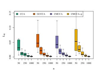
(a)

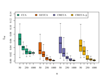
(b)

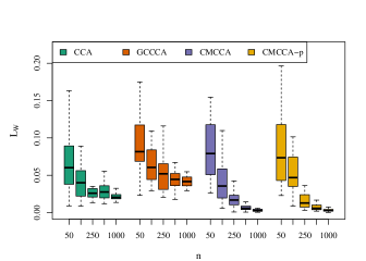
(c)

Figure 1: Mean squared-error for three simulation scenarios and four estimation methods: traditional CCA (CCA), Gaussian copula-based CCA (GCCCA), our method for semiparametric CCA using the multirank likelihood (CMCCA), and semiparametric CCA using plug-in data (CMCCA-p). (a) Estimation improves with sample size for all methods. (b) Estimation with traditional CCA stops improving as $n$ increases. (c) Only the estimators derived from our model for semiparametric CCA improve for $n\geq 250$.

For each simulation scenario, we evaluate four estimation methods: classical CCA, Gaussian copula-based CCA, semiparametric CCA using the multirank likelihood, and semiparametric CCA using the plug-in strategy of Section 3.1. We compare each estimator of the CCA parameters to the true CCA parameters using the loss criterion

$$L_{\boldsymbol{W}}(\hat{\boldsymbol{W}})=\frac{\|\hat{\boldsymbol{W}}-\boldsymbol{W}\|_{2}^{2}}{p_{1}p_{2}}$$

where $\boldsymbol{W}=\boldsymbol{Q}_{1}\boldsymbol{\Lambda}\boldsymbol{Q}_{2}^{\top}$. The precise methods for computing each estimator are detailed in the supplementary file Section B.4. In Figure 1, we show the distribution of $L_{\boldsymbol{W}}(\hat{\boldsymbol{W}})$ for each estimator over $25$ trials for different sample sizes. In the first scenario, the estimation of all four methods improves with sample size. This is expected since the data-generating distribution, the multivariate normal, falls in each of the three model families. In the second scenario, estimation with standard CCA fails to improve with sample size because the data-generating distribution is not normal. However, the data-generating distribution for the second scenario is in the Gaussian copula model and our model for semiparametric CCA, so estimation with each of the corresponding methods improves with sample size. Finally, in the third scenario estimation with standard CCA and estimation with Gaussian copula-based CCA both stop improving as $n$ gets large. Only our model for semiparametric CCA produces estimates that improve with sample size in all three simulation scenarios.

4.2 Analysis of multivariate dependence in two datasets

We further illustrate the use of our method for semiparametric CCA by analyzing multivariate dependence in two datasets. In addition to reporting the magnitude of dependence between variable sets in each dataset, we describe the nature of that dependence through quantitative and qualitative summaries of the posterior distribution of the CCA parameters.

In the first analysis, we consider the association between year-to-year fluctuations of two sets of climate variables measured in five geographic regions of Brazil between 1961 and 2019. These data come from the Brazilian National Institute of Meteorology (INMET) and are available at kaggle.com/datasets. The first group of climate variables consists of temperature, atmospheric pressure, evaporation, insolation, and wind velocity. The second group consists of relative humidity, cloudiness, and precipitation. Individual measurements of the climate variables are averaged across weather stations and across days to obtain average monthly values for each variable within each geographic region. We then take the log ratio between the average value for a given month and the average value in the same month of the previous year to remove seasonal dependence. These log ratios are the observation unit for the climate variables in the analysis that follows.

To determine whether our model for semiparametric CCA should be preferred over traditional CCA or Gaussian copula-based CCA for these data, we apply a normal scores transformation to each climate variable. The normal scores transformation works by aligning the empirical quantiles of each variable with that of the standard normal distribution, transforming data with arbitrary univariate margins to have approximately standard normal margins. If the data have an empirical distribution that is approximately multivariate normal after a normal scores transformation, it would be reasonable to conclude that their distribution can be described by a Gaussian copula. As reported in Table 1 in Section C of the supplementary file, even after the normal scores transformation the climate variables in this sample are not approximately jointly normally distributed according to the Henze-Zirkler test for multivariate normality (Henze and Zirkler,, 1990). However, after applying a multivariate analog of the normal scores transformation (see supplementary file B.5) the climate variables appear to be approximately multivariate normal, indicating that the data may be described by our model for semiparametric CCA.

We apply our method for semiparametric CCA to each region’s climate data by simulating $50,000$ values from a Markov Chain with stationary distribution equal to the posterior distribution of the CCA parameters using the multirank likelihood. We discard the first $5,000$ values and retain every $20^{\text{th}}$ subsequent iterate. Histograms depicting the approximate posterior distributions of $\lambda_{1},\lambda_{2}$, and $\lambda_{3}$ for each geographic region as well as tables reporting posterior means and $95\%$ credible intervals for $\lambda_{1},\lambda_{2}$, and $\lambda_{3}$ can be found in Section C of the supplementary file. These results offer strong evidence that the two climate variable sets are not independent in any of the five regions. However, the results suggest that the dependence in regions 2 and 3 cannot be summarized in fewer than three dimensions, while the dependence in regions 1, 4, and 5 might reasonably be described by a two dimensional model.

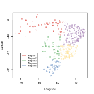
(a)

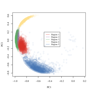
(b)

Figure 2: (a) Geographic locations of weather stations where climate variables were measured, colored by region. (b) Visualization of the posterior distribution of dependence parameters associated with the first canonical correlation for each region.

To further characterize the nature of the dependence between the sets of climate fluctuations, we analyze posterior realizations of $\boldsymbol{O}_{1}=\boldsymbol{q}_{1,1}\boldsymbol{q}_{2,1}^{\top}$, the outer product between the first columns of $\boldsymbol{Q}_{1}$ and $\boldsymbol{Q}_{2}$, for each geographic region. As can be seen in the decomposition

$$\boldsymbol{Q}_{1}\boldsymbol{\Lambda}\boldsymbol{Q}_{2}^{\top}=\sum_{k=1}^{d}\lambda_{k}\boldsymbol{q}_{1,k}\boldsymbol{q}_{2,k}^{\top}=\sum_{k=1}^{d}\lambda_{k}\boldsymbol{O}_{k},$$

$\boldsymbol{O}_{1}$ represents the cross-correlation structure associated with the first canonical correlation. In Figure 2, we display the geographic locations of the weather stations where the climate data were recorded (left) alongside a 2-dimensional principle components projection of the 15-dimensional posterior samples of $\text{vec}(\boldsymbol{O}_{1})$ (right). The posterior distributions indicate that the associations between the climate variable sets in Regions 4 and 5 are quite distinct although they are geographically close, whereas the associations between climate variable sets in Regions 2 and 3 are very similar. A quantitative description of the similarities between the regional dependence structures is found in Table 3 of Section C of the supplementary file, where we report posterior summaries of the cosine similarity between the first canonical axes of each region, defined as

$$\text{CS}(\boldsymbol{O}^{r_{j}}_{1},\boldsymbol{O}^{r_{k}}_{1})=\text{tr}({\boldsymbol{O}^{r_{j}}_{1}}^{\top}\boldsymbol{O}^{r_{k}}_{1})=({\boldsymbol{q}^{r_{j}}_{1,1}}^{\top}\boldsymbol{q}^{r_{k}}_{1,1})({\boldsymbol{q}^{r_{j}}_{2,1}}^{\top}\boldsymbol{q}^{r_{k}}_{2,1})$$

for regions $r_{j}$ and $r_{k}$. Note that this is the same as the inner product used to produce the principle components visualization in Figure 2(b).

The second dataset we analyze, downloaded from finance.yahoo.com, contains monthly log returns of adjusted closing prices of stocks in the materials and communications market sectors from 1985 to 2019. As in Shi et al., (2020), we are interested in detecting dependence between the two sectors. Additionally, we seek to characterize how that dependence differs among three major economic eras in the United States: the period of deregulation and Reaganomics from 1985-1991, the period of technological growth and globalization from 1992-2007, and the aftermath of the Great Recession from 2008-2019. The stocks chosen to represent the materials market sector as classified by Global Industry Classification Standard (GICS) are DuPont de Nemours, Inc. (DD), Olin Corporation (OLN), BHP Group Limited (BHP), and PPG Industries, Inc. (PPG). The stocks chosen to represent the communications sector are Lumen Technologies, Inc. (LUMN), AT&T Inc. (T), Verizon Communications Inc. (VZ), and Comcast Corporation (CMCSA).

Posterior realizations of the CCA parameters for each economic era are obtained with MCMC as in the previous analysis. The posterior distributions of $\lambda_{1},\lambda_{2}$ (Figure 3) indicate that there is dependence between the telecommunications and materials market sectors in all three economic eras. However, they also indicate that this dependence is weaker in the period from 1992-2007 than during the other eras.

Figure 3: Scatter plots of posterior realizations of $\lambda_{1},\lambda_{2}$ for each of three economic eras.

To understand this change in dependence, it may be of interest to interpret how the original variables relate to the canonical variables during each economic era. In traditional applications of CCA, the so-called canonical loadings—the correlation coefficients between each original variable and its corresponding canonical variable—are often reported. As a marginally distribution-free analog, we report the posterior distribution of the sample Spearman rank correlation between each individual stock and its corresponding first canonical variable. Specifically, Table 1 reports the posterior means and $95\%$ credible intervals of

$$\rho_{1,k}=\text{Cor}(R(\boldsymbol{y}_{1,k}),R(\boldsymbol{Z}_{1}\boldsymbol{q}_{1,1})),~{}k=1,\dots,p_{1}$$ (26)

for the materials stocks, where $R(\cdot)$ yields the univariate ranks, $\text{Cor}(\cdot)$ is the Pearson correlation, and $\boldsymbol{y}_{1,k}$ denotes the $k^{\text{th}}$ column of $\boldsymbol{Y}_{1}$. Table 2 reports the corresponding statistic for the communications stocks.

	DD	OLN	BHP	PPG
1985-1991	-0.84, [-0.92, -0.73]	-0.55, [-0.75, -0.31]	-0.20, [-0.52, 0.06]	-0.57, [-0.78, -0.35]
1992-2007	0.53, [0.01, 0.92]	0.56, [0.09, 0.92]	0.56, [0.04, 0.93]	0.57, [0.01, 0.93]
2008-2019	-0.78, [-0.898, -0.65]	-0.44, [-0.62, -0.23]	-0.69, [-0.82, -0.53]	-0.81, [-0.91, -0.71]

Table 1: Sample Spearman correlations (posterior means and $95\%$ credible intervals) between materials stocks and the first canonical variable of the materials stocks variable set.

	LUMN	T	VZ	CMCSA
1985-1991	-0.60, [-0.80, -0.36]	-0.38, [-0.63, -0.11]	-0.38, [-0.64, -0.10]	-0.85, [-0.94, -0.72]
1992-2007	0.62, [0.12, 0.92]	0.42, [-0.13, 0.87]	0.48, [-0.02, 0.92]	0.44, [-0.05, 0.90]
2008-2019	-0.61, [-0.77, -0.46]	-0.44, [-0.66, -0.25]	-0.39, [-0.59, -0.20]	-0.79, [-0.87, -0.67]

Table 2: Sample Spearman correlations (posterior means and $95\%$ credible intervals) between communications stocks and the first canonical variable of the communications stocks variable set.

The results in Tables 1 and 2 support the notion that the nature of the dependence between the materials and communications market sectors differs among the three economic eras. They also provide evidence that the weaker dependence from 1992-2007 is driven by overall market movement, whereas individual stocks such as DD and CMCSA show stronger association to the canonical variables of the first and second variable sets, respectively, in the years before and after this period.

5 Discussion

In this article, we have proposed a semiparametric model for CCA based on cyclically monotone transformations of jointly normal sets of variables. In contrast to existing models for CCA, our model allows the variable sets to have arbitrary multivariate marginal distributions, while retaining a parametric model of dependence. Our main inference approach is based on the multirank likelihood, a type of marginal likelihood, which does not depend on the multivariate marginal distributions of the variable sets. Instead, the multirank likelihood uses information in the cyclically monotone correspondence between the observed data and the unobserved normal latent variables. To simulate values subject to the multirank likelihood’s cyclically monotone constraint, we have also introduced CMMC, which allows us to use the multirank likelihood to obtain both point estimates and confidence regions for the CCA parameters.

Interpreting the CCA parameters in semiparametric CCA presents challenges beyond those of traditional CCA. In our model, the canonical correlations $\boldsymbol{\Lambda}$ may be interpreted as magnitudes of multivariate dependence, just as in traditional CCA. However, the columns of $\boldsymbol{Q}_{1},\boldsymbol{Q}_{2}$ correspond to the latent variable sets $\boldsymbol{Z}_{1},\boldsymbol{Z}_{2}$, and explicitly linking these to the original variables in a manner analogous to the canonical coefficients of traditional CCA requires estimating the transformations $G_{1},G_{2}$. While this is a viable approach, in keeping with the spirit of the rest of the article we have chosen to offer ways of interpreting the CCA parameters without respect to $G_{1},G_{2}$. First, we have demonstrated how the columns of $\boldsymbol{Q}_{1},\boldsymbol{Q}_{2}$ can be compared across populations to obtain similarity measures between those populations, which reflect the type of multivariate dependence observed. Second, we have proposed marginally distribution-free alternatives to canonical loadings, which, like their traditional counterparts, help to interpret the relationship between the original variables and the corresponding canonical variables.

There are several directions of research that could extend this work. For example, much of the recent interest in CCA has been driven by applications in genomics and neuroimaging, for which the variable sets are often high-dimensional compared to the sample size. In these settings, traditional CCA may fail, so it is necessary to use regularized versions of CCA. In principle our approach to semiparametric CCA is amenable to extensions allowing for Bayesian inference in such high-dimensional settings. For instance, regularized CCA could be implemented via shrinkage- or sparsity-inducing prior distributions on the entries of $\boldsymbol{\Lambda}$. In practice, however, scaling the simulation methodology presented here to high-dimensional datasets remains a challenge if the number of canonical correlations is equal to $\min(p_{1},p_{2})$. One useful modification to our model could be to assume that the dependence between variable sets is low-rank by setting $d\ll\min(p_{1},p_{2})$. This would allow our algorithm to scale linearly in $p_{1}$ and $p_{2}$, rather than cubically (see Section B.1.1 of the supplementary file). In this article we presented a coordinate-wise scheme for CMMC. However, hit-and-run schemes for CMMC are also possible, as are those that update several latent variables at once. The cost of computing the regions that preserve cyclical monotonicity remains the primary obstacle to all of these, but there may be exact or approximate CMMC algorithms that could lead to improved mixing times and applicability of CMMC to datasets with larger sample sizes.

Although this article has focused on semiparametric CCA, we anticipate that our inference approach using the multirank likelihood and CMMC will be useful in other semiparametric inference problems, for instance in semiparametric regression or other hierarchical models involving cyclically monotone transformations. Code to reproduce the figures in this article, as well as software for semiparametric CCA as described in this article are available at https://github.com/j-g-b/sbcca.

Acknowledgments

The authors gratefully acknowledge Michael Jauch for helpful comments regarding MCMC methods for orthogonal matrices.

Funding

Jonathan Niles-Weed’s work was supported by the National Science Foundation under Grant DMS-2015291.

Appendix A Proofs of propositions

A.1 Proof of Proposition 2.1

Let $P$ be a probability distribution on $\mathbb{R}^{p}$, and let $\boldsymbol{z}\sim N(\boldsymbol{0},\boldsymbol{I}_{p})$. Further, let

$$\mathcal{G}^{p}=\left\{G~{}|~{}G:\mathbb{R}^{p}\rightarrow\mathbb{R}^{p}\text{ is cyclically monotone}\right\}.$$

Theorems from Brenier, (1991) and McCann, (1995) assert the existence of a convex function $\psi$, unique almost everywhere up to addition of a constant, such that $\nabla\psi$ pushes forward the standard normal distribution on $\mathbb{R}^{p}$ to $P$. Therefore, there exists an almost-everywhere unique $\nabla\psi$ such that

$$\boldsymbol{y}=\nabla\psi(\boldsymbol{z})\sim P.$$

From Rockafellar’s Theorem (Rockafellar,, 1966) we conclude: 1. that $\nabla\psi$ must be cyclically monotone, 2. if there exists a cyclically monotone function $G$ pushing forward the standard normal distribution on $\mathbb{R}^{p}$ to $P$, then the graph of $G$ must coincide with the graph of the gradient of a convex function; hence, by the uniqueness above we must have $G=\nabla\psi$ almost-everywhere. Therefore, there is an almost-everywhere unique $G\in\mathcal{G}^{p}$ so that $\boldsymbol{y}=G(\boldsymbol{z})\sim P$.

A.2 Proof of Proposition 2.2

Let $\boldsymbol{\theta}=(G_{1},G_{2},\boldsymbol{Q}_{1},\boldsymbol{Q}_{2},\boldsymbol{\Lambda})$ and let $P_{\boldsymbol{\theta}}$ denote the joint probability distribution of an observation $(\boldsymbol{y}_{1},\boldsymbol{y}_{2})$ from the model (4) in the main text with $p_{1}$- and $p_{2}$-dimensional marginal distributions $P_{1},P_{2}$. Suppose

$$P_{\boldsymbol{\theta}}=P_{\boldsymbol{\theta}^{\prime}}$$

The equality of the joint probability distributions above implies that the corresponding $p_{1}$- and $p_{2}$- dimensional margins must also be equal. As before, we apply McCann’s Theorem (McCann,, 1995) and Rockafellar’s Theorem (Rockafellar,, 1966) to find that the transformations $G_{1},G_{2}$ pushing forward the $p_{1}$- and $p_{2}$- dimensional standard normal distributions to $P_{1}$, $P_{2}$, respectively, must be unique almost everywhere. Thus,

$$G_{1}=G_{1}^{\prime},~{}~{}G_{2}=G_{2}^{\prime}~{}~{}~{}a.e.$$

Assuming that $P_{1},P_{2}$ are absolutely continuous, McCann’s Theorem (McCann,, 1995) and Rockafellar’s Theorem (Rockafellar,, 1966) also guarantee the existence and almost-everywhere uniqueness of cyclically monotone functions $H_{1},H_{2}$ pushing forward $P_{1}$, $P_{2}$ to the $p_{1}$- and $p_{2}$-dimensional standard normal distributions, respectively. Moreover, $H_{1}\circ G_{1}(\boldsymbol{z}_{1})=\boldsymbol{z}_{1}$ a.e. and $H_{2}\circ G_{2}(\boldsymbol{z}_{2})=\boldsymbol{z}_{2}$ a.e. Applying these functions to $\boldsymbol{y}_{1}$ and $\boldsymbol{y}_{2}$, we obtain

$$\left[\begin{array}[]{c}H_{1}(\boldsymbol{y}_{1})\\ H_{2}(\boldsymbol{y}_{2})\end{array}\right]\sim N_{p_{1}+p_{2}}\left(\boldsymbol{0},\left[\begin{array}[]{cc}\boldsymbol{I}_{p_{1}}&\boldsymbol{Q}_{1}\boldsymbol{\Lambda}\boldsymbol{Q}_{2}^{\top}\\ \boldsymbol{Q}_{2}\boldsymbol{\Lambda}\boldsymbol{Q}_{1}^{\top}&\boldsymbol{I}_{p_{2}}\\ \end{array}\right]\right),$$

and, likewise,

$$\left[\begin{array}[]{c}H_{1}(\boldsymbol{y}_{1}^{\prime})\\ H_{2}(\boldsymbol{y}_{2}^{\prime})\end{array}\right]\sim N_{p_{1}+p_{2}}\left(\boldsymbol{0},\left[\begin{array}[]{cc}\boldsymbol{I}_{p_{1}}&\boldsymbol{Q}_{1}^{\prime}\boldsymbol{\Lambda}^{\prime}{\boldsymbol{Q}^{\prime}_{2}}^{\top}\\ \boldsymbol{Q}_{2}^{\prime}\boldsymbol{\Lambda}^{\prime}{\boldsymbol{Q}_{1}^{\prime}}^{\top}&\boldsymbol{I}_{p_{2}}\\ \end{array}\right]\right),$$

Because $(H_{1}(\boldsymbol{y}_{1}),H_{2}(\boldsymbol{y}_{2}))\overset{d}{=}(H_{1}(\boldsymbol{y}_{1}^{\prime}),H_{2}(\boldsymbol{y}_{2}^{\prime}))$, we obtain

$$\boldsymbol{Q}_{1}\boldsymbol{\Lambda}{\boldsymbol{Q}_{2}}^{\top}=\boldsymbol{Q}_{1}^{\prime}\boldsymbol{\Lambda}^{\prime}{\boldsymbol{Q}^{\prime}_{2}}^{\top}$$

If the diagonal elements of $\boldsymbol{\Lambda},\boldsymbol{\Lambda}^{\prime}$ are strictly decreasing values $[0,1)$, then the uniqueness of the matrix singular value decomposition yields

$$\boldsymbol{\Lambda}=\boldsymbol{\Lambda}^{\prime}$$

and

$$\boldsymbol{Q}_{1}=\boldsymbol{Q}^{\prime}_{1}\boldsymbol{S},\boldsymbol{Q}_{2}=\boldsymbol{Q}^{\prime}_{2}\boldsymbol{S},$$

where $\boldsymbol{S}\in\mathbb{R}^{d\times d}$ is an arbitrary diagonal matrix with diagonal entries in $\left\{-1,1\right\}$. If the entries of $\boldsymbol{\Lambda},\boldsymbol{\Lambda}^{\prime}$ are not strictly decreasing, then the uniqueness of the matrix singular value decomposition yields

$$\boldsymbol{\Lambda}=\boldsymbol{\Lambda}^{\prime}$$

and

$$\boldsymbol{Q}_{1}=\boldsymbol{Q}^{\prime}_{1}\boldsymbol{P}\boldsymbol{S},\boldsymbol{Q}_{2}=\boldsymbol{Q}^{\prime}_{2}\boldsymbol{P}\boldsymbol{S},$$

where $\boldsymbol{P}$ is any permutation matrix with $\boldsymbol{P}_{k}=\boldsymbol{e}_{k}$ if $\lambda_{k}\neq\lambda_{l}~{}\forall l\neq k$ and $\boldsymbol{S}$ is as before.

Appendix B Supplementary details

B.1 Additional details on posterior simulation

Since we use uniform priors for each of the CCA parameters, the full conditional distributions of the CCA parameters are derived from densities proportional to the density of the latent variables $\boldsymbol{Z}_{1},\boldsymbol{Z}_{2}$ given the CCA parameters. This is the $n\times(p_{1}+p_{2})$ matrix normal density with the CCA parameterization truncated to the set $\{\mathbf{Z}:\mathbf{Z}\overset{\mathrm{cm}}{\sim}\mathbf{Y}\}$. The log of this density is

$$\log\left(\Gamma_{CCA}(\mathbf{Z};\boldsymbol{Q}_{1},\boldsymbol{Q}_{2},\boldsymbol{\Lambda})\mathbb{I}[\mathbf{Z}\overset{\mathrm{cm}}{\sim}\mathbf{Y}]\right) =-\frac{n}{2}\log|\boldsymbol{I}-\boldsymbol{\Lambda}|$$

$$-\frac{1}{2}\text{tr}\left(\mathbf{Z}_{1}\mathbf{Z}_{1}^{\top}+\mathbf{Z}_{2}\mathbf{Z}_{2}^{\top}\right)$$

$$-\frac{1}{2}\text{tr}\left(\mathbf{Z}_{1}\mathbf{Q}_{1}(\boldsymbol{\Lambda}^{-2}-\mathbf{I})^{-1}\mathbf{Q}_{1}^{\top}\mathbf{Z}_{1}^{\top}+\mathbf{Z}_{2}\mathbf{Q}_{2}(\boldsymbol{\Lambda}^{-2}-\mathbf{I})^{-1}\mathbf{Q}_{2}^{\top}\mathbf{Z}_{2}^{\top}\right)$$

$$-\text{tr}\left(\mathbf{Z}_{1}\mathbf{Q}_{1}(\boldsymbol{\Lambda}-\boldsymbol{\Lambda}^{-1})^{-1}\mathbf{Q}_{2}^{\top}\mathbf{Z}_{2}^{\top}\right)$$

$$+\log\mathbb{I}[\mathbf{Z}\overset{\mathrm{cm}}{\sim}\mathbf{Y}].$$

Eliminating terms that are constant in each variable yields the full conditional distributions given in the main text.

The full conditional distribution for $\boldsymbol{\Lambda}$ has an exponential family form, but it is not clear how to simulate directly from it. Therefore, we use a Metropolis-Hastings algorithm to simulate each $\lambda_{k}$. We propose new values according to

$$\lambda_{k}^{*}\sim N\left(r_{k},\frac{1}{n}\left(1-\frac{2c_{k}}{a_{k}+b_{k}}\right)\right),$$

truncated to the region $\lambda_{k-1}\geq\lambda_{k}^{*}\geq\lambda_{k+1}$, where $r_{k}$ is the real root to the cubic equation

$$\lambda_{k}^{3}-\frac{c_{k}}{n}\lambda_{k}^{2}+\frac{a_{k}+b_{k}-n}{n}\lambda_{k}-\frac{c_{k}}{n}=0,$$

and $\boldsymbol{a},\boldsymbol{b}$ and $\boldsymbol{c}$ are defined as in (11) from the main text. This equation is obtained by setting the derivative of the logarithm of the full conditional density for $\lambda_{k}$ to zero, so that $r_{k}$ is the mode of the full conditional distribution for $\lambda_{k}$.

Simulation of $\boldsymbol{Q}_{1},\boldsymbol{Q}_{2}$ is accomplished by iterating a Markov Chain for auxiliary variables $\boldsymbol{X}_{1},\boldsymbol{X}_{2}$ and taking $\boldsymbol{Q}_{1},\boldsymbol{Q}_{2}$ to be the left polar factors of these matrices at each iteration as in Jauch et al., (2021). Specifically, if $\boldsymbol{X}_{1}^{*}$ is a proposed value for $\boldsymbol{X}_{1}$, then

$$\boldsymbol{Q}_{1}^{*}=\boldsymbol{U}^{*}\boldsymbol{V}^{*\top},$$

where $\boldsymbol{U}^{*},\boldsymbol{V}^{*}$ are the left and right singular vectors of $\boldsymbol{X}^{*}$. Elliptical slice sampling (Murray et al.,, 2010) is an MCMC method applicable to simulating from posterior distributions proportional to the product of a normal prior distribution and a likelihood function. Since the matrix normal prior distributions $\boldsymbol{X}_{1}\sim N_{p_{1}\times d}(\boldsymbol{0},\boldsymbol{I}_{d}\otimes\boldsymbol{I}_{p_{1}})$ and $\boldsymbol{X}_{2}\sim N_{p_{2}\times d}(\boldsymbol{0},\boldsymbol{I}_{d}\otimes\boldsymbol{I}_{p_{2}})$ induce uniform prior distributions on the Stiefel manifolds $\mathcal{V}_{p_{1},d},\mathcal{V}_{p_{2},d}$, we are able to use elliptical slice sampling to simulate new values for $\boldsymbol{X}_{1},\boldsymbol{X}_{2}$ at each iteration, where $\log\Gamma_{CCA}(\mathbf{Z};\boldsymbol{Q}_{1},\boldsymbol{Q}_{2},\boldsymbol{\Lambda})$ is the log likelihood function used in the slice sampling algorithm.

B.1.1 Computational complexity

The singular value decompositions needed to simulate values of $\boldsymbol{Q}_{1},\boldsymbol{Q}_{2}$ scale with complexity $O(d^{2}(p_{1}+p_{2}))=O(\min(p_{1},p_{2})^{3})$. As described in the main text, CMMC scales as $O(n^{2}(p_{1}+p_{2}))$. The order of both these terms dominates the complexity of the matrix multiplications required for the rest of the simulation methodology, so the overall computational cost of our method scales as $O(T(\min(p_{1},p_{2})^{3}+n^{2}(p_{1}+p_{2})))$ where $T$ is the number of iterates in the Markov Chain. The cubic term in the dimension of the smallest variable set presents a challenge to scaling our method to higher dimensions. A solution to this problem is proposed in the discussion of Section 5 of the main text.

B.2 Missing data and mixed data

The algorithm for estimation of the CCA parameters can be modified to accommodate data missing at random (MAR). For instance, if $\boldsymbol{y}_{i,1}$ is missing, then the multirank likelihood does not impose a cyclically monotone constraint on $\boldsymbol{z}_{i,1}$. The CMMC algorithm can therefore be initialized by solving an assignment problem between $\mathbf{Y}_{-i,1}$ and $\mathbf{Z}_{-i,1}^{(0)}$. Then, at each iteration, a new value for $\boldsymbol{z}_{i,1}$ can be simulated from the full conditional distribution

$$\boldsymbol{z}_{i,1}|-\sim N_{p_{1}}(\boldsymbol{Q}_{1}\boldsymbol{\Lambda}\boldsymbol{Q}_{2}^{\top}\boldsymbol{z}_{i,2},\boldsymbol{I}_{p_{1}}-\boldsymbol{Q}_{1}\boldsymbol{\Lambda}^{2}\boldsymbol{Q}_{1}^{\top}).$$

When simulating values in a CMMC step for the other latent variables, the constraints in (17) and (19) of the main text can be computed over $\mathbf{Y}_{-i,1}$. The case of multiple missing rows in either $\boldsymbol{Y}_{1}$ or $\boldsymbol{Y}_{2}$ may be treated analogously. The situation of individual entries missing, however, is more complicated and requires imputation under the MAR assumption. We reserve this case for future work on sampling with cyclically monotone constraints.

In contrast to methods based on the multivariate ranks of Chernozhukov et al., (2017), in principle the multirank likelihood can be used in a Bayesian inference procedure with data of mixed type, including binary, count, or proportion data. However, it is not yet clear how much information about the CCA parameters is lost when the margins are discrete. Further work is needed to establish results on identifiability in the case of multivariate marginals that are not absolutely continuous.

B.3 Discussion of multirank terminology

A rank likelihood is a likelihood function equivalent to the sampling distribution of the univariate ranks of random variables. For instance, consider the bivariate copula model for $\boldsymbol{z}_{1},\boldsymbol{z}_{2}\in\mathbb{R}^{n}$:

$$[\boldsymbol{z}_{1}~{}\boldsymbol{z}_{2}] \sim N\left(\boldsymbol{0},\left[\begin{array}[]{cc}1&\rho\\ \rho&1\end{array}\right]\otimes\boldsymbol{I}_{n}\right)$$

$$y_{i,j} =g_{j}(z_{i,j}),~{}i=1,\dots,n,~{}j=1,2$$

where $g_{j}$ is an absolutely continuous, monotone increasing function. Define the univariate rank function $R:\mathbb{R}^{n}\rightarrow\{1,\dots,n\}^{n}$, so that the $i^{\text{th}}$ element of $R(\boldsymbol{y}_{j})$ is the rank of $y_{i,j}$ among $\{y_{1,j},\dots,y_{n,j}\}$. If the observed data values have ranks $R(\mathbf{y}_{1})=\mathbf{r}_{1},R(\mathbf{y}_{2})=\mathbf{r}_{2}$, then the rank likelihood for the dependence parameter $\rho$ is

$$\text{Pr}(R(\boldsymbol{y}_{1})=\mathbf{r}_{1},R(\boldsymbol{y}_{2})=\mathbf{r}_{2}|\rho).$$

Note that the probability distribution for $R(\boldsymbol{y}_{1}),R(\boldsymbol{y}_{2})$ does not depend on the transformation functions $g_{1},g_{2}$, which makes the rank likelihood useful for semiparametric estimation of dependence.

In the multivariate case, one can define a multirank likelihood equivalent to the sampling distribution of a multivariate rank statistic. Indeed, the multirank likelihood for the semiparametric CCA model in the main text is an example of such a multirank likelihood. Defining the appropriate multivariate rank statistic is less straightforward than in the univariate case, but it can be done as follows: let $P$ be an absolutely continuous probability distribution on $\mathbb{R}^{p}$. McCann’s Theorem (McCann,, 1995) and Rockafellar’s Theorem (Rockafellar,, 1966) guarantee the existence and almost-everywhere uniqueness of a cyclically monotone function $H$ pushing forward $P$ to the $p$-dimensional standard normal distribution. Let $\mathbf{M}\in\mathbb{R}^{n\times p}$ be a fixed matrix. Define the map $t_{H,\mathbf{M}}:\mathbb{R}^{n\times p}\rightarrow S_{n}$ by

$$t_{H,\mathbf{M}}(\boldsymbol{Y})=\underset{\sigma=(\sigma(1),\dots,\sigma(n))\in S_{n}}{\arg\min}\sum_{i=1}^{n}\|\mathbf{m}_{\sigma(i)}-H(\boldsymbol{y}_{i})\|_{2}^{2},$$

where $S_{n}$ is the permutation group on $\{1,\dots,n\}$, and let $\sigma_{0}$ be the identity permutation.

Now, suppose that $\boldsymbol{Z}\sim N(0,\boldsymbol{I}_{p}\otimes\boldsymbol{I}_{n})$, and suppose that $G$ is the almost-everywhere unique cyclically monotone function pushing forward the $p$-dimensional standard normal distribution to $P$. Then if $\boldsymbol{y}_{i}=G(\boldsymbol{z}_{i}),~{}i=1,\dots,n$, the following hold with probability 1:

1. $\boldsymbol{Z}\overset{\mathrm{cm}}{\sim}\mathbf{M}\implies H(\boldsymbol{Y})\overset{\mathrm{cm}}{\sim}\mathbf{M}\implies t_{H,\mathbf{M}}(\boldsymbol{Y})=\sigma_{0}.$

2. $t_{H,\mathbf{M}}(\boldsymbol{Y})=\sigma_{0}\implies H(\boldsymbol{Y})\overset{\mathrm{cm}}{\sim}\mathbf{M}\implies\boldsymbol{Z}\overset{\mathrm{cm}}{\sim}\mathbf{M}$.

Therefore, with probability 1,

$$\boldsymbol{Z}\overset{\mathrm{cm}}{\sim}\mathbf{M}\iff t_{H,\mathbf{M}}(\boldsymbol{Y})=\sigma_{0}.$$

We define the $i^{\text{th}}$ element of $t_{H,\mathbf{M}}(\boldsymbol{Y})$ to be the multirank of $\boldsymbol{y}_{i}$. In the context of the semiparametric CCA model, the multirank likelihood from the main text is equivalent to the joint distribution of the multiranks of the variable sets $\boldsymbol{Y}_{1},\boldsymbol{Y}_{2}$:

$$L_{M}(\boldsymbol{Q}_{1},\boldsymbol{Q}_{2},\boldsymbol{\Lambda}:\mathbf{Y}) =\text{Pr}(\boldsymbol{Z}_{1}\overset{\text{cm}}{\sim}\mathbf{Y}_{1},\boldsymbol{Z}_{2}\overset{\text{cm}}{\sim}\mathbf{Y}_{2}|\boldsymbol{Q}_{1},\boldsymbol{Q}_{2},\boldsymbol{\Lambda})$$

$$=\text{Pr}(t_{H_{1},\mathbf{Y}_{1}}(\boldsymbol{Y}_{1})=\sigma_{0},t_{H_{2},\mathbf{Y}_{2}}(\boldsymbol{Y}_{2})=\sigma_{0}|\boldsymbol{Q}_{1},\boldsymbol{Q}_{2},\boldsymbol{\Lambda})$$

B.4 Estimators for the CCA parameters in the simulation study

Here we describe the steps used to compute each estimator in the simulation study of Section 4.1 in the main text.

B.4.1 Traditional CCA

1. Compute

   1. $\hat{\boldsymbol{\Sigma}}_{1}=\frac{1}{n}(\boldsymbol{Y}_{1}-\frac{1}{n}\boldsymbol{1}\boldsymbol{1}^{\top}\boldsymbol{Y}_{1})^{\top}(\boldsymbol{Y}_{1}-\frac{1}{n}\boldsymbol{1}\boldsymbol{1}^{\top}\boldsymbol{Y}_{1})$

   2. $\hat{\boldsymbol{\Sigma}}_{2}=\frac{1}{n}(\boldsymbol{Y}_{2}-\frac{1}{n}\boldsymbol{1}\boldsymbol{1}^{\top}\boldsymbol{Y}_{2})^{\top}(\boldsymbol{Y}_{2}-\frac{1}{n}\boldsymbol{1}\boldsymbol{1}^{\top}\boldsymbol{Y}_{2})$

   3. $\hat{\boldsymbol{\Omega}}=\frac{1}{n}(\boldsymbol{Y}_{1}-\frac{1}{n}\boldsymbol{1}\boldsymbol{1}^{\top}\boldsymbol{Y}_{1})^{\top}(\boldsymbol{Y}_{2}-\frac{1}{n}\boldsymbol{1}\boldsymbol{1}^{\top}\boldsymbol{Y}_{2})$

2. Set $\hat{\boldsymbol{W}}=\hat{\boldsymbol{\Sigma}}_{1}^{-1/2}\hat{\boldsymbol{\Omega}}\hat{\boldsymbol{\Sigma}}_{2}^{-1/2}$

B.4.2 Gaussian copula-based CCA

1. Simulate 500 posterior samples of $\boldsymbol{C}$, the $(p_{1}+p_{2})\times(p_{1}+p_{2})$-dimensional correlation matrix parametrizing a Gaussian copula using the R package sbgcop.

2. For each posterior sample, set $\boldsymbol{\Sigma}^{(t)}_{1},\boldsymbol{\Sigma}^{(t)}_{2},\boldsymbol{\Omega}^{(t)}$ to be the upper $p_{1}\times p_{1}$ block, lower $p_{2}\times p_{2}$ block, and $p_{1}\times p_{2}$ off-diagonal block, respectively, of $\boldsymbol{C}^{(t)}$.

3. Compute $\boldsymbol{W}^{(t)}={\boldsymbol{\Sigma}^{(t)}_{1}}^{-1/2}\boldsymbol{\Omega}^{(t)}{\boldsymbol{\Sigma}^{(t)}_{2}}^{-1/2}$ for each posterior sample.

4. Compute posterior mean $\hat{\boldsymbol{W}}=\frac{1}{T}\sum_{t=1}^{T}\boldsymbol{W}^{(t)}$.

B.4.3 Semiparametric CCA using the multirank likelihood

1. Simulate 500 posterior samples of $\boldsymbol{Q}_{1},\boldsymbol{Q}_{2},\boldsymbol{\Lambda}$ using the simulation methodology of Section 3.3.

2. Compute the product $\boldsymbol{W}^{(t)}=\boldsymbol{Q}^{(t)}_{1}\boldsymbol{\Lambda}^{(t)}{\boldsymbol{Q}^{(t)}_{2}}^{\top}$ for each posterior sample.

3. Compute posterior mean $\hat{\boldsymbol{W}}=\frac{1}{T}\sum_{t=1}^{T}\boldsymbol{W}^{(t)}$.

B.4.4 Semiparametric CCA using plug-in data

1. Simulate matrices $\boldsymbol{Z}_{1},\boldsymbol{Z}_{2}$ with i.i.d. standard normal entries.

2. Permute the rows of $\boldsymbol{Z}_{1}$ and $\boldsymbol{Z}_{2}$ so that the permuted matrices $\hat{\boldsymbol{Z}}_{1}$ and $\hat{\boldsymbol{Z}}_{2}$ are in cycically monotone correspondence with $\boldsymbol{Y}_{1},\boldsymbol{Y}_{2}$, respectively.

3. Compute

   1. $\hat{\boldsymbol{\Sigma}}_{1}=\frac{1}{n}(\hat{\boldsymbol{Z}}_{1}-\frac{1}{n}\boldsymbol{1}\boldsymbol{1}^{\top}\hat{\boldsymbol{Z}}_{1})^{\top}(\hat{\boldsymbol{Z}}_{1}-\frac{1}{n}\boldsymbol{1}\boldsymbol{1}^{\top}\hat{\boldsymbol{Z}}_{1})$

   2. $\hat{\boldsymbol{\Sigma}}_{2}=\frac{1}{n}(\hat{\boldsymbol{Z}}_{2}-\frac{1}{n}\boldsymbol{1}\boldsymbol{1}^{\top}\hat{\boldsymbol{Z}}_{2})^{\top}(\hat{\boldsymbol{Z}}_{2}-\frac{1}{n}\boldsymbol{1}\boldsymbol{1}^{\top}\hat{\boldsymbol{Z}}_{2})$

   3. $\hat{\boldsymbol{\Omega}}=\frac{1}{n}(\hat{\boldsymbol{Z}}_{1}-\frac{1}{n}\boldsymbol{1}\boldsymbol{1}^{\top}\hat{\boldsymbol{Z}}_{1})^{\top}(\hat{\boldsymbol{Z}}_{2}-\frac{1}{n}\boldsymbol{1}\boldsymbol{1}^{\top}\hat{\boldsymbol{Z}}_{2})$

4. Set $\hat{\boldsymbol{W}}=\hat{\boldsymbol{\Sigma}}_{1}^{-1/2}\hat{\boldsymbol{\Omega}}\hat{\boldsymbol{\Sigma}}_{2}^{-1/2}$

B.5 Multivariate normal scores transformation

We calculate multivariate normal scores in Section 4.2 of the main text using the following steps:

1. Simulate matrices $\boldsymbol{Z}_{1},\boldsymbol{Z}_{2}$ with i.i.d. standard normal entries.

2. Obtain the optimal assignments between $\boldsymbol{Z}_{1},\boldsymbol{Y}_{1}$ and $\boldsymbol{Z}_{2},\boldsymbol{Y}_{2}$.

3. Permute the rows of $\boldsymbol{Z}_{1}$ and $\boldsymbol{Z}_{2}$ to obtain the multivariate normal scores $\hat{\boldsymbol{Z}}_{1}$ and $\hat{\boldsymbol{Z}}_{2}$, which are in cycically monotone correspondence with $\boldsymbol{Y}_{1},\boldsymbol{Y}_{2}$, respectively.

Appendix C Additional tables and figures

	Region 1	Region 2	Region 3	Region 4	Region 5
H-Z statistic (normal scores)	1.3959217	1.3183332	1.3622823	1.3925435	0.9476107
p-value (normal scores)	$<10^{-7}$	$<10^{-7}$	$<10^{-7}$	$<10^{-7}$	0.4643700
H-Z statistic (m.v. normal scores)	0.9403996	0.9848370	0.9951354	0.9774440	0.9305933
p-value (m.v. normal scores)	0.9151626	0.2004779	0.1055596	0.2731933	0.7070755

Table 3: Results of Henze-Zirkler test for multivariate normality on regional climate fluctuations after applying a normal scores transformation (top two rows) and after applying a multivariate normal scores transformation (bottom two rows).

	Region 1	Region 2	Region 3	Region 4	Region 5
$\lambda_{1}$	0.81 [0.75, 0.88]	0.96 [0.93, 0.99]	0.92 [0.88, 0.95]	0.92 [0.87, 0.97]	0.77 [0.56, 0.95]
$\lambda_{2}$	0.24 [0.10, 0.39]	0.62 [0.51, 0.73]	0.63 [0.54, 0.72]	0.44 [0.28, 0.60]	0.24 [0.02, 0.46]
$\lambda_{3}$	0.13 [0, 0.24]	0.18 [0.02, 0.33]	0.22 [0.08, 0.36]	0.09 [0, 0.21]	0.1 [0, 0.26]

Table 4: Posterior means and $95\%$ credible intervals for $\lambda_{1},\lambda_{2},\lambda_{3}$ for each geographic region in Brazil.

	Region 2	Region 3	Region 4	Region 5
Region 1	0.80, [0.69, 0.90]	0.83, [0.73, 0.93]	0.65, [0.46, 0.82]	0.52, [0.26, 0.78]
Region 2	.	0.95, [0.90, 0.99]	0.84, [0.72, 0.95]	0.54, [0.29, 0.78]
Region 3	.	.	0.84, [0.70, 0.97]	0.55, [0.31, 0.83]
Region 4	.	.	.	0.24, [0.01, 0.49]

Table 5: Cosine similarity (posterior means and $95\%$ credible intervals) between the first canonical axes of climate fluctuations of each geographic region in Brazil.

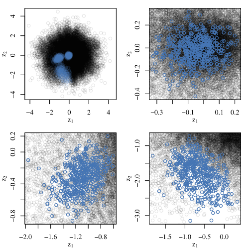
Figure 4: Sample output from CMMC. Top left: scatterplot of 500 posterior simulations of each observation of a two-dimensional latent variable set. Posterior simulations of $\boldsymbol{z}_{i},~{}i=1,\dots,100$ are plotted in transparent black, while the posterior samples of three randomly selected $\boldsymbol{z}_{i}$’s are highlighted in blue. Top right: close-up of the posterior simulations of the first highlighted $\boldsymbol{z}_{i}$. Bottom left: close-up of the posterior simulations of the second highlighted $\boldsymbol{z}_{i}$. Bottom right: close-up of the posterior simulations of the third highlighted $\boldsymbol{z}_{i}$. Note that the posterior densities of the $\boldsymbol{z}_{i}$’s highlighted in blue are concentrated around certain regions, but they clearly overlap with the regions of high density for other $\boldsymbol{z}_{i}$’s.

Figure 5: Autocorrelation plots computed on 500 posterior samples of 5 randomly selected entries of the latent variables and CCA parameters using the same run as in Figure 1, for which one variable set is two-dimensional and one variable set is five-dimensional. These were obtained after retaining every 10${}^{\text{th}}$ iterate of a larger sample of 5,000 posterior realizations.

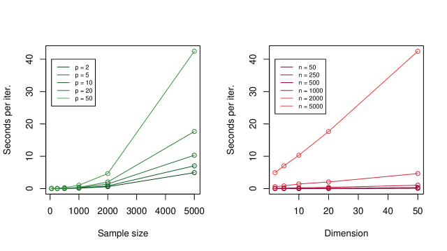
Figure 6: Empirical time per iteration for our implementation (run on a 2017 MacBook Pro using R version 4.0.5) of MCMC for the CCA parameters. Times are plotted as a function of $n$ (left) and $p=p_{1}=p_{2}$ (right).

Figure 7: Histograms of posterior realizations of $\lambda_{1},\lambda_{2},\lambda_{3}$ for each of the five geographic regions in Brazil. Dotted lines denote the boundaries of $95\%$ credible intervals.

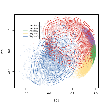
Figure 8: Visualization of the posterior distribution of dependence parameters associated with the second canonical correlation for each geographic region in Brazil.

References

- Agniel and Cai, (2017) Agniel, D. and Cai, T. (2017). Analysis of multiple diverse phenotypes via semiparametric canonical correlation analysis. Biom, 73(4):1254–1265.
- Ambrosio and Gigli, (2013) Ambrosio, L. and Gigli, N. (2013). A User’s Guide to Optimal Transport. In Modelling and Optimisation of Flows on Networks, volume 2062, pages 1–155. Springer Berlin Heidelberg, Berlin, Heidelberg.
- Anderson, (1999) Anderson, T. (1999). Asymptotic Theory for Canonical Correlation Analysis. Journal of Multivariate Analysis, 70(1):1–29.
- Bach and Jordan, (2005) Bach, F. R. and Jordan, M. I. (2005). A probabilistic interpretation of canonical correlation analysis. Technical report.
- Bakirov et al., (2006) Bakirov, N. K., Rizzo, M. L., and Székely, G. J. (2006). A multivariate nonparametric test of independence. Journal of Multivariate Analysis, 97(8):1742–1756.
- Brenier, (1991) Brenier, Y. (1991). Polar factorization and monotone rearrangement of vector-valued functions. Comm. Pure Appl. Math., 44(4):375–417.
- Chen et al., (2013) Chen, J., Bushman, F. D., Lewis, J. D., Wu, G. D., and Li, H. (2013). Structure-constrained sparse canonical correlation analysis with an application to microbiome data analysis. Biostatistics, 14(2):244–258.
- Chernozhukov et al., (2017) Chernozhukov, V., Galichon, A., Hallin, M., and Henry, M. (2017). Monge–Kantorovich depth, quantiles, ranks and signs. Ann. Statist., 45(1).
- Deb et al., (2021) Deb, N., Bhattacharya, B. B., and Sen, B. (2021). Efficiency Lower Bounds for Distribution-Free Hotelling-Type Two-Sample Tests Based on Optimal Transport. arXiv:2104.01986 [math, stat]. arXiv: 2104.01986.
- Deb and Sen, (2021) Deb, N. and Sen, B. (2021). Multivariate Rank-Based Distribution-Free Nonparametric Testing Using Measure Transportation. Journal of the American Statistical Association, pages 1–16.
- del Barrio et al., (2020) del Barrio, E., González-Sanz, A., and Hallin, M. (2020). A note on the regularity of optimal-transport-based center-outward distribution and quantile functions. Journal of Multivariate Analysis, 180:104671.
- Dempster et al., (1977) Dempster, A. P., Laird, N. M., and Rubin, D. B. (1977). Maximum Likelihood from Incomplete Data Via the EM Algorithm. Journal of the Royal Statistical Society: Series B (Methodological), 39(1):1–22.
- Eaton, (1983) Eaton, M. L. (1983). Multivariate statistics: a vector space approach. Wiley series in probability and mathematical statistics. Wiley, New York.
- Fan and Henry, (2020) Fan, Y. and Henry, M. (2020). Vector copulas and vector Sklar theorem. arXiv:2009.06558 [econ, math, stat]. arXiv: 2009.06558.
- Figalli, (2018) Figalli, A. (2018). On the continuity of center-outward distribution and quantile functions. Nonlinear Analysis, 177:413–421.
- Gelfand and Smith, (1990) Gelfand, A. E. and Smith, A. F. M. (1990). Sampling-Based Approaches to Calculating Marginal Densities. Journal of the American Statistical Association, 85(410):398–409.
- Genest et al., (1995) Genest, C., Ghoudi, K., and Rivest, L.-P. (1995). A semiparametric estimation procedure of dependence parameters in multivariate families of distributions. Biometrika, 82(3):543–552.
- Hallin, (2017) Hallin, M. (2017). On Distribution and Quantile Functions, Ranks and Signs in R_d. Working Papers ECARES ECARES 2017-34, ULB – Universite Libre de Bruxelles.
- Henze and Zirkler, (1990) Henze, N. and Zirkler, B. (1990). A class of invariant consistent tests for multivariate normality. Communications in Statistics - Theory and Methods, 19(10):3595–3617.
- Hoff, (2007) Hoff, P. D. (2007). Extending the rank likelihood for semiparametric copula estimation. Ann. Appl. Stat., 1(1):265–283.
- Hoff, (2009) Hoff, P. D. (2009). Simulation of the Matrix Bingham–von Mises–Fisher Distribution, With Applications to Multivariate and Relational Data. Journal of Computational and Graphical Statistics, 18(2):438–456.
- Hoff et al., (2014) Hoff, P. D., Niu, X., and Wellner, J. A. (2014). Information bounds for Gaussian copulas. Bernoulli, 20(2).
- Hotelling, (1936) Hotelling, H. (1936). Relations Between Two Sets of Variates. Biometrika, 28(3/4):321.
- Jauch et al., (2021) Jauch, M., Hoff, P. D., and Dunson, D. B. (2021). Monte Carlo Simulation on the Stiefel Manifold via Polar Expansion. Journal of Computational and Graphical Statistics, pages 1–10.
- Jendoubi and Strimmer, (2019) Jendoubi, T. and Strimmer, K. (2019). A whitening approach to probabilistic canonical correlation analysis for omics data integration. BMC Bioinformatics, 20(1):15.
- Mardia et al., (1979) Mardia, K. V., Kent, J. T., and Bibby, J. M. (1979). Multivariate analysis. Probability and mathematical statistics. Academic Press, London ; New York.
- McCann, (1995) McCann, R. J. (1995). Existence and uniqueness of monotone measure-preserving maps. Duke Math. J., 80(2):309–323.
- Murray et al., (2010) Murray, I., Adams, R., and MacKay, D. (2010). Elliptical slice sampling. In Teh, Y. W. and Titterington, M., editors, Proceedings of the Thirteenth International Conference on Artificial Intelligence and Statistics, volume 9 of Proceedings of Machine Learning Research, pages 541–548, Chia Laguna Resort, Sardinia, Italy. PMLR.
- Oakes, (1994) Oakes, D. (1994). Multivariate survival distributions. Journal of Nonparametric Statistics, 3(3-4):343–354.
- Pan et al., (2020) Pan, W., Wang, X., Zhang, H., Zhu, H., and Zhu, J. (2020). Ball Covariance: A Generic Measure of Dependence in Banach Space. Journal of the American Statistical Association, 115(529):307–317.
- Peyré and Cuturi, (2018) Peyré, G. and Cuturi, M. (2018). Computational Optimal Transport. arXiv:1803.00567 [stat]. arXiv: 1803.00567.
- Rockafellar, (1966) Rockafellar, R. (1966). Characterization of the subdifferentials of convex functions. Pacific J. Math., 17(3):497–510.
- Severini, (2000) Severini, T. A. (2000). Likelihood methods in statistics. Number 22 in Oxford statistical science series. Oxford University Press, Oxford ; New York.
- Sherry and Henson, (2005) Sherry, A. and Henson, R. K. (2005). Conducting and Interpreting Canonical Correlation Analysis in Personality Research: A User-Friendly Primer. Journal of Personality Assessment, 84(1):37–48.
- Shi et al., (2020) Shi, H., Drton, M., and Han, F. (2020). Distribution-Free Consistent Independence Tests via Center-Outward Ranks and Signs. Journal of the American Statistical Association, pages 1–16.
- Winkler et al., (2020) Winkler, A. M., Renaud, O., Smith, S. M., and Nichols, T. E. (2020). Permutation inference for canonical correlation analysis. NeuroImage, 220:117065.
- Yoon et al., (2020) Yoon, G., Carroll, R. J., and Gaynanova, I. (2020). Sparse semiparametric canonical correlation analysis for data of mixed types. Biometrika, 107(3):609–625.
- Zoh et al., (2016) Zoh, R. S., Mallick, B., Ivanov, I., Baladandayuthapani, V., Manyam, G., Chapkin, R. S., Lampe, J. W., and Carroll, R. J. (2016). PCAN: Probabilistic correlation analysis of two non‐normal data sets. Biom, 72(4):1358–1368.