A Tutorial on Optimal Control and Reinforcement Learning methods for Quantum Technologies

Abstract

Quantum Optimal Control is an established field of research which is necessary for the development of Quantum Technologies. In recent years, Machine Learning techniques have been proved usefull to tackle a variety of quantum problems. In particular, Reinforcement Learning has been employed to address typical problems of control of quantum systems. In this tutorial we introduce the methods of Quantum Optimal Control and Reinforcement Learning by applying them to the problem of three-level population transfer. The jupyter notebooks to reproduce some of our results are open-sourced and available on github2.

1 Introduction

In the last two decades many advances have been made in the field of Quantum Technology (QT). QT aims at developing practical applications by making use of the properties of quantum mechanics, such as superposition and entanglement [1]. The ability to precisely manipulate quantum systems is a key tool in developing quantum technologies [1, 2, 3, 4, 5].

Quantum Control (QC) looks at providing the user with a set of time-dependent control parameters in order to drive a dynamical quantum system such that it performs some specific task [2, 3, 4, 5].

Optimal Control Theory (OCT) is a field of applied mathematics and is a powerful tool that provides methods to find controls that allow a dynamical system to evolve to achieve a predefined goal. For reference textbooks see for example [6, 7, 8]. When this theory is applied to quantum systems it is often referred to as Quantum Optimal Control (QOC) [2, 3, 4, 5]. However there are other techniques such as Transitionless Quantum Driving [9] (or Shortcut to Adiabaticity [10]).

More recently the overlap between the fields of machine learning and quantum mechanics have been explored extensively [11, 12, 13, 14, 15], with both machine learning algorithms used to improve the understanding and the control of quantum systems [16, 17, 18], and properties of quantum mechanics used to improve machine learning algorithms (Quantum Machine Learning) [19, 20, 21]. In particular, reinforcement learning (RL) has been employed in the context of control of multi-level systems [22, 23, 24], and for quantum sensing and metrology [25, 26, 27].

In this tutorial we illustrate the methods of numerical Optimal Control and Reinforcement Learning by applying them to the problem of population transfer in a three-level $\Lambda$ or ladder system, for which a well-known solution is STIRAP [28, 29, 30]. Analytical solutions to this problem via Optimal Control have been presented in [31, 32, 3] and a numerical example is given in [33, 34], but, to our knowledge, no systematic numerical study exists. This problem has also been studied by applying Reinforcement Learning in [23, 24]. Here we improve those results by defining the Markov Decision Process in a more convenient way, using a simpler Reinforcement Learning algorithm, reaching the solution by training the model for fewer episodes and reaching an overall better fidelity.

The paper is organized as follows: in Sec. 2 we introduce the problem of three-level population transfer and its solution via STIRAP. In Sec. 3 we introduce Optimal Control Theory and show its application on three-level population transfer. In Sec. 4 we introduce the Reinforcement Learning paradigm and show its application to the same problem. Finally, in Sec. 5 we draw the conclusions.

We open-source parts of the source code we produced. It is easily adaptable, with minor changes, to different situations involving population transfer in three-level systems.

2 Three-level population transfer

Consider a three-level system composed of the quantum states $\{|g\rangle,|e\rangle,|r\rangle\}$ with energies $\{\hbar\omega_{\mathrm{g}},\hbar\omega_{\mathrm{e}},\hbar\omega_{\mathrm{r}}\}$. The transition $g\leftrightarrow e$ is driven by a classical field (called pump field) with frequency $\omega_{\mathrm{p}}$ and Rabi frequency $\Omega_{\mathrm{p}}(t)$. The transition $e\leftrightarrow r$ is driven by another classical field (called Stokes field) at frequency $\omega_{\mathrm{s}}$ and Rabi frequency $\Omega_{\mathrm{s}}(t)$, see Fig. 1. Both Rabi frequencies $\Omega_{\mathrm{p}}(t)$ and $\Omega_{\mathrm{s}}(t)$ can vary with time.

Figure 1: Scheme of the three-level system. (a) $\Lambda$ structure and (b) ladder structure.

The process we want to achieve consists in transferring the population from state $|g\rangle$ to state $|r\rangle$ by suitably shaping the Rabi frequencies $\Omega_{\mathrm{p}}(t)$ and $\Omega_{\mathrm{s}}(t)$ in time.

In the following sections we introduce the equations that describe the dynamics of the system, and the STIRAP [28, 29, 30] protocol which allows an efficient transfer of population.

2.1 Master equation

In the rotating wave approximation [35, 36] and in a convenient rotating frame the Hamiltonian reads [29]

$$\frac{H(t)}{\hbar}={} \Delta_{\mathrm{p}}\left|e\right>_{\!}\left<e\right|+\Delta_{3}\left|r\right>_{\!}\left<r\right|+\frac{\Omega_{\mathrm{p}}(t)}{2}\left(\left|g\right>_{\!}\left<e\right|+\left|e\right>_{\!}\left<g\right|\right)+{}$$ (1)

$$+\frac{\Omega_{\mathrm{s}}(t)}{2}\left(\left|e\right>_{\!}\left<r\right|+\left|r\right>_{\!}\left<e\right|\right)$$

where the detunings from the resonances are defined as $\Delta_{\mathrm{p}}=\omega_{\mathrm{p}}-(\omega_{\mathrm{e}}-\omega_{\mathrm{g}})$, $\Delta_{\mathrm{s}}=\omega_{\mathrm{s}}-\left|\omega_{\mathrm{r}}-\omega_{\mathrm{e}}\right|$, and $\Delta_{3}=\Delta_{\mathrm{p}}-\Delta_{\mathrm{s}}$ for the $\Lambda$ configuration, and $\Delta_{3}=\Delta_{\mathrm{p}}+\Delta_{\mathrm{s}}$ for the ladder configuration, see Fig. 1. While single-photon resonance is not required in order to obtain a nearly perfect transfer, the two-photon resonance is usually required [29] (apart some peculiar cases such as Ref. [18]). Thus we allow the single-photon detuning to be different from zero $\Delta_{\mathrm{p}}\neq 0$, while we assume the two-photon detuning to be zero $\Delta_{3}=0$ for the rest of this manuscript. We also assume the Rabi frequencies $\Omega_{\mathrm{p}}(t)$ and $\Omega_{\mathrm{s}}(t)$ to be real since their phase could be for example absorbed in the definition of the states $|g\rangle$ and $|r\rangle$ [36]. If the system under consideration is an atomic or molecular system, then the Rabi frequencies are given by $\Omega_{\mathrm{p}}(t)=-d_{\mathrm{ge}}\mathcal{E}_{\mathrm{p}}(t)/\hbar$ and $\Omega_{\mathrm{s}}(t)=-d_{\mathrm{er}}\mathcal{E}_{\mathrm{s}}(t)/\hbar$, where $d_{mn}$ are the components of the dipole-transition moments along their respective electric-field vectors, and $\mathcal{E}_{\mathrm{s/p}}(t)$ are the slowly varying amplitudes of the pump and Stokes electric fields [30].

In both the configurations $\Lambda$ and ladder (see Fig. 1), the excited states can undergo spontaneous emission to lower-lying states. Those emission processes that lead to levels outside the three-level system determine a probability loss and thus are undesirable. Spontaneous emission processes back to state $|g\rangle$ or $|r\rangle$ are incoherent and thus are also undesirable.

In this work we only consider radiative decay from the excited state $|e\rangle$ to states outside the three-level system. We model this phenomenon by a Born-Markov process described by the superoperator $\mathcal{L}_{\gamma}$ such that the master equation describing the time evolution of the density matrix $\rho(t)$ reads [37]

$$\dot{\rho}(t)=-\frac{\mathrm{i}}{\hbar}[H(t),\rho(t)]+\mathcal{L}_{\gamma}\rho(t),$$ (2)

with

$$\mathcal{L}_{\gamma}\rho(t)=\frac{\gamma}{2}\left(2\left|s\right>_{\!}\left<e\right|\rho(t)\left|e\right>_{\!}\left<s\right|-\left|e\right>_{\!}\left<e\right|\rho(t)-\rho(t)\left|e\right>_{\!}\left<e\right|\right).$$ (3)

Here $|s\rangle$ is an auxiliary state where the population losses at rate $\gamma$ from state $|e\rangle$ are collected.

The figure of merit we use to quantify the performance of a protocol is the fidelity defined as

$$\mathcal{F}=\lim_{t\to\infty}\operatorname*{Tr}\left\{\rho(t)\left|r\right>_{\!}\left<r\right|\right\}.$$ (4)

It is clear that a perfect protocol would have fidelity $\mathcal{F}=1$.

2.2 Review of the STIRAP protocol

STImulated Raman Adiabatic Passage (STIRAP) [28, 29, 30] is an adiabatic protocol that allows population transfer from state $|g\rangle$ to state $|r\rangle$ with fidelity close to one by keeping the population on the lossy state $|e\rangle$ very low during the evolution. In order to explain the STIRAP protocol we first introduce the adiabatic theorem [38, 39].

2.2.1 Adiabatic theorem

Given a time-dependent Hamiltonian $H_{0}(t)$, its instantaneous eigenstates $|n(t)\rangle$ and its instantaneous eigenenergies $E_{n}(t)$ are given by

$$H_{0}(t)|n(t)\rangle=E_{n}(t)|n(t)\rangle,$$ (5)

i.e., they are obtained by diagonalizing the Hamiltonian $H_{0}(t)$ at each time step $t$. For simplicity lets assume all the states $|n(t)\rangle$ to be non-degenerate for any $t$. The solution of the time-dependent Schrödinger equation

$$\mathrm{i}\hbar\frac{\partial|\psi(t)\rangle}{\partial t}=H_{0}(t)|\psi(t)\rangle,$$ (6)

is in general a linear combination of all the instantaneous eigenstates

$$|\psi(t)\rangle=\sum_{n}c_{n}(t)|n(t)\rangle,$$ (7)

where $c_{n}(t)$ are time-dependent complex amplitudes and $\sum_{n}\left|c_{n}(t)\right|^{2}=1$.

If the Hamiltonian $H_{0}(t)$ is slowly varying and the initial state is one of the instantaneous eigenstates, then the adiabatic theorem guarantees that the system will follow that instantaneous eigenstate closely: during the time evolution of the system, the transition amplitudes to instantaneous eigenstates different from the starting one are approximately to zero (see Fig. 2 for an artistic representation of this concept). If the initial state is $|\psi(t_{\mathrm{i}})\rangle=|m(t_{\mathrm{i}})\rangle$, then

$$|\psi(t)\rangle\simeq\mathrm{e}^{\mathrm{i}\alpha_{m}(t)}|m(t)\rangle,$$ (8)

i.e., $c_{n}(t)\simeq\mathrm{e}^{\mathrm{i}\alpha_{m}(t)}\delta_{mn}$, where $\alpha(t)$ is a global phase which is not important for our discussion.

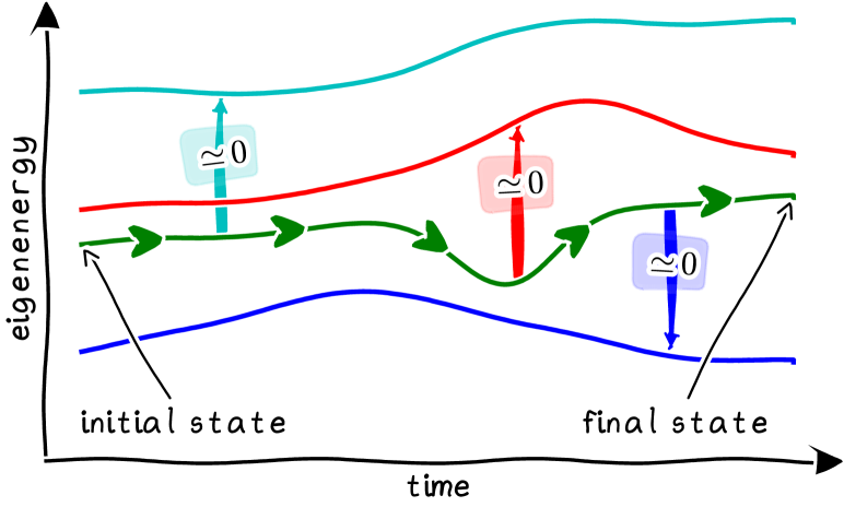
Figure 2: Artistic view of adiabatic following of an instantaneous eigenstate. The colored boxes represent the transition probabilities which are approximately zero in an adiabatic process.

The condition for the Hamiltonian $H_{0}(t)$ to be considered slowly varying can be obtained by imposing that the probability of finding the system in a state $|m(t)\rangle$ different from the initial state $|n(t_{\mathrm{i}})\rangle$ is small. This can be written as [39]

$$\hbar\left|\langle n(t)|\partial_{t}m(t)\rangle\right|\ll\left|E_{n}(t)-E_{m}(t)\right|,\forall m\neq n.$$ (9)

We proceed by calculating the instantaneous eigenenergies and eigenstates (i.e., the eigensystem) of Hamiltonian $H(t)$ reported in eq. (1).

2.2.2 Eigensystem of $H(t)$

The analysis of the three-level dynamics can be written in a simpler form by defining

$$\Omega_{0}(t)=\sqrt{\Omega_{\mathrm{p}}(t)^{2}+\Omega_{\mathrm{s}}(t)^{2}},$$ (10a)

$$\tan\theta(t)=\frac{\Omega_{\mathrm{p}}(t)}{\Omega_{\mathrm{s}}(t)},$$ (10b)

$$\tan\phi(t)=\frac{\Omega_{0}(t)}{\Delta_{\mathrm{p}}+\sqrt{\Delta_{\mathrm{p}}^{2}+\Omega_{0}(t)^{2}}}.$$ (10c)

The instantaneous eigenvalues of Hamiltonian $H(t)$, eq. (1) (with $\Delta_{3}=0$) are [29]

$$\lambda_{0}(t)=0,$$ (11a)

$$\lambda_{-}(t)=-\frac{\hbar}{2}\Omega_{0}(t)\tan\phi(t),$$ (11b)

$$\lambda_{+}(t)=\frac{\hbar}{2}\Omega_{0}(t)\cot\phi(t),$$ (11c)

and the relative instantaneous eigenstates are

$$|a_{0}(t)\rangle=\cos\theta(t)|g\rangle-\sin\theta(t)|r\rangle,$$ (12a)

$$\begin{aligned} |a_{-}(t)\rangle={}&\sin\theta(t)\cos\phi(t)|g\rangle-\sin\phi(t)|e\rangle+{}\\ &+\cos\theta(t)\cos\phi(t)|r\rangle,\end{aligned}$$ (12b)

$$\begin{aligned} |a_{+}(t)\rangle={}&\sin\theta(t)\sin\phi(t)|g\rangle+\cos\phi(t)|e\rangle+{}\\ &+\cos\theta(t)\sin\phi(t)|r\rangle.\end{aligned}$$ (12c)

As the three-level key feature, the $|a_{0}\rangle$ eigenstate with eigenvalue zero is a dark state [40] with zero projection on state $|e\rangle$.

2.2.3 STIRAP

The STIRAP protocol allows for an efficient population transfer from state $|g\rangle$ to state $|r\rangle$ by adiabatically following the dark state $|a_{0}\rangle$. Since the state $|a_{0}\rangle$, eq. (12a), does not have any component along the excited state $|e\rangle$, the population losses at rate $\gamma$ from that state have very little impact on the evolution of the system and thus on the fidelity $\mathcal{F}$ of the process.

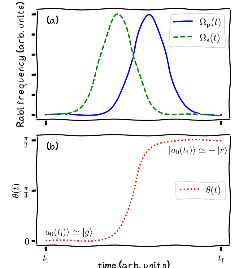
Figure 3: Counter-intuitive sequence of pulses peculiar to the STIRAP protocol. (a) Pump and Stokes gaussian pulses of the type $\Omega_{\mathrm{p/s}}(t)\propto\mathrm{e}^{-\left[(t\mp\tau)/T\right]^{2}}$, and (b) time dependence of $\theta(t)$ given by eq. (10b) with the Rabi frequencies of (a).

In order to achieve population transfer from state $|g\rangle$ to state $|r\rangle$ by following $|a_{0}(t)\rangle$ we need

$$|a_{0}(t_{\mathrm{i}})\rangle \propto|g\rangle,$$ (13a)

$$|a_{0}(t_{\mathrm{f}})\rangle \propto|r\rangle,$$ (13b)

where $t_{\mathrm{i}}$ and $t_{\mathrm{f}}$ are the initial and final time, respectively. This is obtained if the Stokes and pump pulses satisfy

$$\lim_{t\to t_{\mathrm{i}}}\tan\theta(t)=\lim_{t\to t_{\mathrm{i}}}\frac{\Omega_{\mathrm{p}}(t)}{\Omega_{\mathrm{s}}(t)}=0,$$ (14a)

$$\lim_{t\to t_{\mathrm{f}}}\cot\theta(t)=\lim_{t\to t_{\mathrm{f}}}\frac{\Omega_{\mathrm{s}}(t)}{\Omega_{\mathrm{p}}(t)}=0,$$ (14b)

and, equivalently $\lim_{t\to t_{\mathrm{i}}}\theta(t)=0,\ \lim_{t\to t_{\mathrm{f}}}\theta(t)=\pm\pi/2$.

In order for the evolution to be adiabatic, the pulses must also satisfy the condition [29, 41]

$$|\dot{\theta}(t)|\ll\frac{1}{2}\left|\Delta_{\mathrm{p}}\pm\sqrt{\Delta_{\mathrm{p}}^{2}+\Omega_{0}(t)^{2}}\right|,$$ (15)

which is obtained by applying eq. (9) to the eigensystem given in eqs. (11) and (12). Eq. (15) is a local adiabaticity condition and must be valid for every time $t$.

Eqs. (14) and (15) mathematically formalize the concept of counter-intuitive pulse sequence peculiar to the STIRAP protocol: the Stokes pulse (which couples the initially empty states $|e\rangle$ and $|r\rangle$) is applied first, then it gets slowly turned off while the pump pulse is turned on, having an overlap with the Stokes pulse. Being and adiabatic protocol, STIRAP is very robust against noise in the control fields [30].

Typically used pulses are of the form

$$\Omega_{\mathrm{p}}(t)=\Omega_{\mathrm{max}}f\left(\frac{t-\tau}{T}\right),\quad\Omega_{\mathrm{s}}(t)=\alpha\Omega_{\mathrm{max}}f\left(\frac{t+\tau}{T}\right),$$ (16)

where $f(t)$ is a pulse envelope having unit maximum value, $\Omega_{\mathrm{max}}$ is the peak Rabi frequency, $2\tau$ is the delay between the pulses, $T$ is the pulse width, and $\alpha$ is a scaling parameter usually equal to $1$. The counter-intuitive sequence condition imposes $\tau>0$.

By assuming $\Delta_{\mathrm{p}}\ll\Omega_{\mathrm{p}}(t),\Omega_{\mathrm{s}}(t)$, a global adiabaticity condition is derived by time averaging eq. (15) over the characteristic time $\tau$ of the $\Omega_{\mathrm{p}}(t)$ and $\Omega_{\mathrm{s}}(t)$ overlap. For the pulses of eq. (16) using eqs. (14) the global adiabaticity condition becomes $\Omega_{\mathrm{max}}\tau\gg 1$.

An example of STIRAP pulses is plotted in Fig. 3. For a list of various pulse shapes used in literature and the relative superadiabatic solution we refer to [42, 43].

Finding new STIRAP-like protocols is important in solid-state systems where often one must operate with reduced control resources [44, 45] since they provide new tools for coherently probing [46, 47] or for processing [48] in quantum architectures.

3 Optimal Control

In this section we introduce the Optimal Control problem and one way to approach its solution numerically. For a more rigorous and general treatment we refer the reader to the classical books [7, 6] and the introductory reviews [3, 4, 5].

3.1 Formulation of the Optimal Control problem

Consider a system described by the (non-linear) set of differential equations

$$\begin{gathered}\dot{\rho}(t)=f\left(\rho(t),\boldsymbol{u}(t),t\right),\quad t\in[0,T],\\ \boldsymbol{u}(t)=\left(u_{1}(t),u_{2}(t),\dots,u_{M}(t)\right),\end{gathered}$$ (17)

where $\rho(t)$ represents the state of the system, $f$ is a smooth function which describes the dynamics of the state $\rho(t)$ and depends on the $M$ control functions $\boldsymbol{u}(t)$. The objective of optimal control is to find some control functions $\boldsymbol{u}(t)$ such that the dynamics of the system is as close as possible to the desired dynamics (examples of what this means will be explicitly given later). This is done by introducing a cost functional

$$\mathcal{J}(\rho(t),\boldsymbol{u}(t),T)$$ (18)

whose minimization corresponds to the desired dynamics.

3.1.1 Quantum Optimal Control

Quantum Control consists in the control of the evolution of a quantum system. We can formulate the quantum control problem as

$$\dot{\rho}(t)=\mathcal{L}(t,\boldsymbol{u}(t))\rho(t),$$ (19)

i.e., by identifying in eq. (17) $\rho(t)$ with the density matrix, $f$ with a super-operator that acts on the space of density matrices and that describes the time evolution of the system, and $\boldsymbol{u}(t)$ with some external controls. The time evolution of the system can be expressed as

$$\rho(t)=R(t,\boldsymbol{u}(t))\rho(0),$$ (20)

where with $R(t,\boldsymbol{u}(t))$ we indicate the time-evolution superoperator (or quantum map) which does not need to be unitary since it can describe both the coherent and incoherent dynamics [49].

The Quantum Optimal Control problem consists in determining the control amplitudes $\boldsymbol{u}(t)$ that will perform the quantum operation of interest, e.g. drive the system from the given initial state $\rho(0)$ at time $t=0$ to the target state $\rho_{\mathrm{targ}}$ at time $t=T$ (this process is called state transfer), or that implements a transformation $R_{\mathrm{targ}}$ in the time interval $[0,T]$ (gate synthesis).

To quantify how close the evolution given by $R(t,\boldsymbol{u}(t))$ is to the target evolution we define a cost functional $\mathcal{J}$ (as in eq. (18)) that we seek to minimize, with respect to the controls $\boldsymbol{u}(t)$. $\mathcal{J}(\rho(t),\boldsymbol{u}(t),T)$ being minimal should correspond to the ideal process we want to perform. Commonly used functionals for quantum processes are of the form

$$\mathcal{J}(\rho(t),\boldsymbol{u}(t),T)=1-\mathcal{F}$$ (21)

where $\mathcal{F}$ is the transfer fidelity [54, 4, 5]

$$\mathcal{F}=\operatorname*{Tr}\left\{\rho_{\mathrm{targ}}^{\dagger}\rho(T)\right\},$$ (22)

for the case of state transfer, and the gate fidelity [55, 56, 57, 51, 4, 5, 58]

$$\mathcal{F}=d^{-1}\left|\operatorname*{Tr}\left\{R_{\mathrm{targ}}^{\dagger}R(T,\boldsymbol{u}(t))\right\}\right|,$$ (23)

where $d$ is the dimension of the Hilbert space of the system, for the case of gate synthesis.

Notice that the final time $T$ can be fixed, or can be included in the functional in order to minimize also the duration of a quantum process.

Constraints on the controls can also be included in the definition of the cost functional $\mathcal{J}$ [3, 4, 5, 59] but we do not consider them here.

3.1.2 Hamiltonian Control

A typical situation encountered in quantum control is when each control amplitude $u_{j}(t)$ in $\boldsymbol{u}(t)$ corresponds to an external tunable parameter which can be described by Hermitian operator in the Hamiltonian. For the purpose of this tutorial we assume that the dynamics of the system can be described by the Lindblad master equation [60, 61]

$$\dot{\rho}(t)=\mathcal{L}(t)\rho(t)=-\mathrm{i}[H(t),\rho(t)]+\mathcal{L}_{\mathrm{dis}}\rho(t),$$ (24)

where the Hamiltonian $H(t)$ describes the coherent dynamics and $\mathcal{L}_{\mathrm{dis}}$ the incoherent dynamics. The Hamiltonian can be written as

$$H(t)=H_{0}+\sum_{k=1}^{M}u_{k}(t)H_{k},$$ (25)

where $H_{0}$ is the free evolution Hamiltonian (often called drift Hamiltonian), $H_{k}$ for $k=1,\dots,M$ are the available control Hamiltonians corresponding to operations on the system we can control, and $u_{k}(t)$ are the time-varying amplitude functions for their relative control. The solution of eq. (24) can be written as

$$\rho(t)=R(t,\boldsymbol{u}(t))[\rho(0)],$$ (26a)

$$R(t,\boldsymbol{u}(t))=\mathcal{T}\exp{\int_{0}^{t}\mathcal{L}(t^{\prime})\mathrm{d}t^{\prime}}$$ (26b)

$$\boldsymbol{u}(t)=\left(u_{1}(t),u_{2}(t),\dots,u_{M}(t)\right),$$ (26c)

and $\mathcal{T}$ is the time-ordering operator.

To summarize, we now want to find a set of controls $\boldsymbol{u}(t)$ such that the evolution of the system given by eqs. (26) is the target evolution. To quantify how close the system evolution is to the target one, we need to minimize the cost functional in eq. (21) with eqs. (22) or (23).

Once the problem has been defined, a method for minimizing the cost functional $\mathcal{J}$ is required. Various strategies exist to solve this problem, both analytical methods based on calculus of variations and the Pontryagins minimum principle [3], and numerical methods. In this tutorial we focus exclusively on numerical methods.

3.2 Numerical solution of the Quantum Optimal Control problem

The numerical solution of the Quantum Optimal Control problem requires the mapping of the cost function $\mathcal{J}$, eq. (18), to a multivariate real function $\bar{\mathcal{J}}$, and then numerically minimize $\bar{\mathcal{J}}$.

The mapping is done by parametrizing each control amplitude $u_{k}(t)$ with $N_{k}$ real numbers, i.e. with a vector $\boldsymbol{\alpha}_{k}\in\mathbb{R}^{N}_{k}$. This is done by approximating each $u_{k}(t)$ as an expansion on a finite set of functions as in

$$u_{k}(t)=\sum_{j=1}^{N_{k}^{\prime}}c_{kj}\chi_{kj}(t,\boldsymbol{d}_{kj}),$$ (27)

where $\chi_{kj}(t,\boldsymbol{d}_{kj})$ are time-dependent functions which depend on the parameters $\boldsymbol{d}_{kj}$, and

$$\boldsymbol{\alpha}_{k}=\{\Re\left(c_{kj}\right),\Im\left(c_{kj}\right),\Re\left(\boldsymbol{d}_{kj}\right),\Im\left(\boldsymbol{d}_{kj}\right)\}_{j=1,\dots,N_{k}^{\prime}}$$

are the $N_{k}$ parameters representing the function $u_{k}(t)$. Notice that we can choose a different set of function $\chi_{kj}$ for each control $u_{k}(t)$.

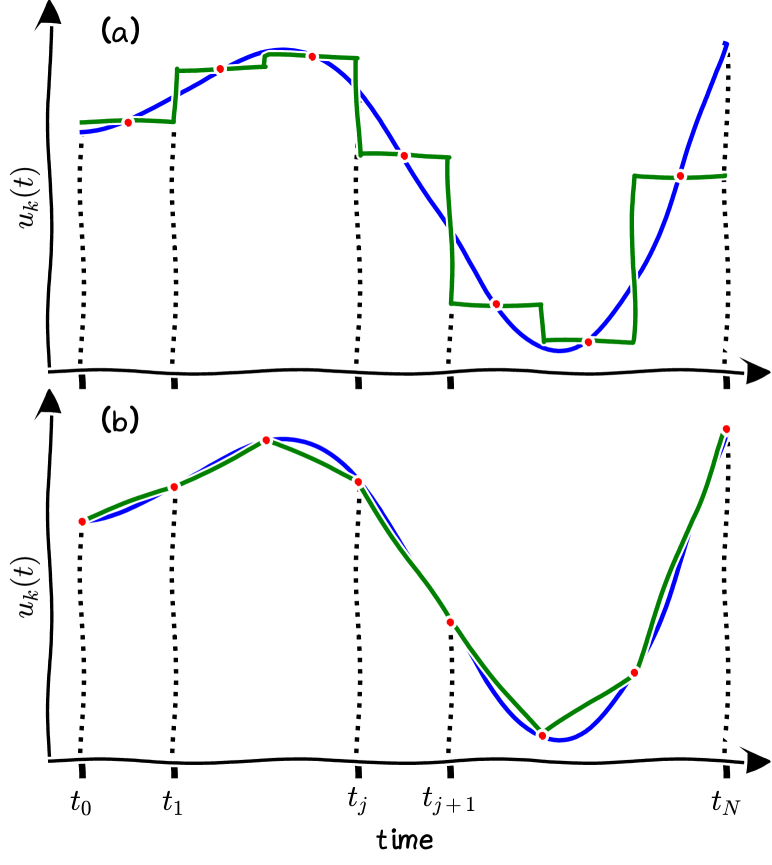
Figure 4: Artistic view of piecewise (a) constant and (b) linear functions that can approximate the real control amplitude $u_{k}(t)$.

A useful and simple set of functions which can be used to expand the control amplitudes are piecewise functions: we split the time interval $[0,T]$ in $N^{\prime}$ smaller intervals $I_{j}$ of length $\Delta t=T/N^{\prime}$ as in the following:

$$I_{j}=[t_{j-1},t_{j}),\quad j=1,\dots,N^{\prime},$$ (28)

such that $t_{0}=0$, $t_{N^{\prime}}=T$, and $t_{j}=t_{j-1}+\Delta t$. With this time discretization we can define

$$\chi_{kj}(t,\boldsymbol{d}_{kj})=\begin{cases}f_{kj}(t,\boldsymbol{d}_{kj})&t\in I_{j}\\ 0&\text{otherwise}\end{cases}$$ (29)

where $f_{kj}$ are some (possibly) time-dependent functions. The functions $\chi_{kj}(t,\boldsymbol{d}_{kj})$ are different from zero only in the interval $I_{j}$, such that the function $u_{k}$ is equal to the function $f_{kj}(t,\boldsymbol{d}_{kj})$ in the interval $I_{j}$.

An important set of functions often used are step functions (or piecewise constant functions): In some problems (such as state transfer and gate synthesis as described above) they decrease the computational cost of calculating the gradient [54] and thus speed up the numerical minimization using gradient-based algorithms. They are obtained by choosing $f_{kj}(t,\boldsymbol{d}_{kj})=1$ in eq. (29), then $u_{k}(t)$ can be easily written as

$$u_{k}(t)=\begin{cases}c_{kj}&t\in I_{j}\\ 0&\text{otherwise}.\end{cases}$$ (30)

The $N=2N^{\prime}$ real parameters representing the function $u_{k}(t)$ can be chosen to be

$$\boldsymbol{\alpha}_{k}=(\Re\left(c_{k1}\right),\dots,\Re\left(c_{kN^{\prime}}\right),\Im\left(c_{k1}\right),\dots,\Im\left(c_{kN^{\prime}}\right)).$$

If we assume the function $u_{k}(t)$ to be real, then $N=N^{\prime}$ and $\boldsymbol{\alpha}_{k}=(c_{k1},c_{k2},\dots,c_{kN^{\prime}})$. Notice that eq. (30) is the nearest-neighbor constant interpolation of the points $\boldsymbol{\alpha}_{k}=(c_{k1},c_{k2},\dots,c_{kN^{\prime}})$, see Fig. 4(a).

If $f_{kj}$ are linear functions and we impose $u_{k}(t)$ to be continuous, then

$$f_{kj}(t,\boldsymbol{d}_{kj})=\frac{c_{k(j-1)}}{c_{kj}}+\frac{c_{kj}-c_{k(j-1)}}{c_{kj}\Delta t}(t-t_{j-1}),$$ (31)

with $\boldsymbol{d}_{kj}=\{c_{k(j-1)},c_{kj}\}$. In this case the control function $u_{k}(t)$ can be easily written as

$$u_{k}(t)=\begin{cases}c_{k(j-1)}+\frac{c_{kj}-c_{k(j-1)}}{\Delta t}(t-t_{j-1})&t\in I_{j}\\ 0&\text{otherwise}.\end{cases}$$ (32)

If we assume that the function $u_{k}(t)$ is real, then it can be parametrized by $N=N^{\prime}+1$ real parameters $\boldsymbol{\alpha}_{k}=(c_{k0},c_{k1},\dots,c_{kN^{\prime}})$. Notice that eq. (32) is the linear interpolation of the points $\boldsymbol{\alpha}_{k}=(c_{k0},c_{k1},\dots,c_{kN^{\prime}})$, see Fig. 4(b).

3.2.1 Final minimization

Once we have chosen a parametrization of the functions $\boldsymbol{u}(t)$ we collect all the parameters $\boldsymbol{\alpha}_{k}\in\mathbb{R}^{N}$ of all the functions $u_{k}(t)$ for $k=1,\dots,M$ into a single vector $\boldsymbol{\alpha}\in\mathbb{R}^{N\times M}$ so that we can write the cost functional as

$$\mathcal{J}(\rho(t),\boldsymbol{u}(t),T)=\bar{\mathcal{J}}(\rho(t),\boldsymbol{\alpha},T)$$ (33)

where in $\bar{\mathcal{J}}$ the evolution of $\rho(t)$ is computed with the control amplitudes parametrized by $\boldsymbol{\alpha}$. Now it is possible to minimize $\bar{\mathcal{J}}(\rho(t),\boldsymbol{\alpha},T)$ with respect to the $N\times M$ real parameters using any of the numerical methods developed to minimize multivariate real functions.

An issue that is often encountered in the minimization process consists in the algorithm being stuck in a local minimum: usually the numerical algorithms will find the local minimum which is the closest to the starting point (called initial guess). While increasing the number of parameters can potentially solve this problem [62], several methods have also been developed in order to address this issue, see for example [63, 64, 65]. A simple approach is to try different initial guesses and choose the minimization which gives the minimum value of $\bar{\mathcal{J}}$.

Several methods have been developed in order to speed up the minimization of the cost function $\bar{\mathcal{J}}$. They use properties of the dynamics of the systems in order to decrease the computational cost of calculating its gradient, or choose a suitable set of functions $\chi_{kj}$ in order to speed up the convergence of the minimization algorithm, or to reduce the dimensionality of the optimization problem [66]. Here we list some of the most common algorithms, while we refer the reader to the original paper or the recent reviews [4, 5] for a deeper explanation: GRAPE [54], Krotov [67, 68, 69, 70], GOAT [71], CRAB [72, 73, 74], dCRAB [75].

3.3 Three-level population transfer

We now formulate the three-level population transfer process introduced in section 2 as an Optimal Control problem and solve it numerically.

Following eq. (25) we identify in eq. (1) the drift Hamiltonian ($\hbar=1$) as

$$H_{0}=\Delta_{\mathrm{p}}\left|e\right>_{\!}\left<e\right|+\Delta_{3}\left|r\right>_{\!}\left<r\right|$$ (34)

and the control Hamiltonians as

with $u_{1}(t)=\Omega_{\mathrm{p}}(t)$ and $u_{2}(t)=\Omega_{\mathrm{s}}(t)$. We assume the controls $\Omega_{\mathrm{p}}(t)$ and $\Omega_{\mathrm{s}}(t)$ to be real constant piecewise functions and parametrize each of them with $N$ parameters corresponding to the value they assume on each time interval, see sec. 3.2 and in particular eqs. (28) and (30). We collect the $2N$ parameters in the vector $\boldsymbol{\alpha}\in\mathbb{R}^{2N}$.

Our goal is to find the control amplitudes $\Omega_{\mathrm{p}}(t)$ and $\Omega_{\mathrm{s}}(t)$ that maximize the population on the state $|\psi_{\mathrm{targ}}\rangle=|r\rangle$ at time $t=T$ starting from the state $|\psi(0)\rangle=|g\rangle$ at time $t=0$. Thus we define the cost function $\mathcal{J}(\rho(t),\boldsymbol{u}(t),T)$ as in eqs. (21) and (22), i.e.:

$$\bar{\mathcal{J}}(\rho(t),\boldsymbol{\alpha},T)=\mathcal{J}(\rho(t),\boldsymbol{u}(t),T)=1-\operatorname*{Tr}\left\{\rho_{\mathrm{targ}}^{\dagger}\rho(T)\right\},$$ (35)

where $\rho_{\mathrm{targ}}=\left|\psi_{\mathrm{targ}}\right>_{\!}\left<\psi_{\mathrm{targ}}\right|=\left|r\right>_{\!}\left<r\right|$ with $\rho(T)$ obtained from the evolution following the master equation (2) (equivalently eq. (24)) with the initial density matrix being $\rho(0)=\left|g\right>_{\!}\left<g\right|$.

3.3.1 Results

We minimize $\bar{\mathcal{J}}(\rho(t),\boldsymbol{\alpha},T)$ with respect to $\alpha$ numerically, with $N=30$. Since the problem is easy (it consists in solving numerically a system of $16$ coupled linear differential equations, which we do numerically with QuTiP [76]) we do not use any advanced method. We have tried the Powell method [77], the Nelder-Mead algorithm [78], and the limited memory BFGS bounded (L-BFGS-B) method [79] as implemented by SciPy [80]. We present the results obtained with L-BFGS-B since we have found that it is the fastest (with Nelder-Mead being the slowest).

The maximum efficiency of the protocol depends on the constraints given by the time of the transfer $T$, the decay rate $\gamma$, and the maximum allowed Rabi frequency $\Omega_{\mathrm{max}}$. However, since there is a freedom on the choice of the unit of time (or equivalently the unit of frequency), the system is invariant under a transformation that keeps $T\gamma$ and $T\Omega_{\mathrm{max}}$ constant, i.e., if

$$\begin{cases}T^{\prime}=\alpha T,\\ \gamma^{\prime}=\gamma/\alpha,\\ \Omega_{\mathrm{max}}^{\prime}=\Omega_{\mathrm{max}}/\alpha,\end{cases}$$ (36)

then the system with parameters $(T,\gamma,\Omega_{\mathrm{max}})$ is mathematically equivalent to the system with $(T^{\prime},\gamma^{\prime},\Omega_{\mathrm{max}}^{\prime})$. In particular the fidelities $\mathcal{F}(T,\gamma,\Omega_{\mathrm{max}})=\mathcal{F}(T^{\prime},\gamma^{\prime},\Omega_{\mathrm{max}}^{\prime})=\mathcal{F}(T\gamma,T\Omega_{\mathrm{max}})$ are the same. Thus in the following we will report the results as a function of $T\gamma$ and $T\Omega_{\mathrm{max}}$.

Fig. 5 reports the inefficiency of the optimized protocol with respect to $T\Omega_{\mathrm{max}}$ for various values of the decay rate $T\gamma$.

Figure 5: Inefficiency $1-\mathcal{F}$, eq. (22) of the optimized protocol, as a function of $T\Omega_{\mathrm{max}}$, for various values of $T\gamma$. For each point we have optimized with $4$ different initial guesses and chosen the best one. The $3$ red empty circles refer to the parameters used in Fig. 6.

Figure 6: Example of optimized pulses and evolution for $T\gamma=5$. The top panels (a-c) report the optimized pulses $\Omega_{\mathrm{p}}(t)$ and $\Omega_{\mathrm{s}}(t)$, the lower panels (d-f) report the population of the states of the system when driven by the pulses in (a-c), respectively. For (a) and (d) $T\Omega_{\mathrm{max}}=7.4$, for (b) and (e) $T\Omega_{\mathrm{max}}=13.8$, and for (c) and (f) $T\Omega_{\mathrm{max}}=100$. We have also chosen $\Omega_{\mathrm{p}}(t)$ and $\Omega_{\mathrm{s}}(r)$ to be real and $N=30$.

The red circles on the $T\gamma=5$ line refer to the points represented in Fig. 6. For all values of $T\Omega_{\mathrm{max}}$ the optimized pulses recall the typical counter-intuitive pulse sequence of STIRAP: for values of $T\Omega_{\mathrm{max}}\lesssim 40$ the optimized pulses present an initial and final maximum interleaved by the counter-intuitive sequence. The area of this initial and final short bumps decreases with increasing $T\Omega_{\mathrm{max}}$. For $T\Omega_{\mathrm{max}}\gtrsim 40$ the pulses are exactly counter-intuitive and they tend to maximize the area at their disposal and their overlap still meeting the condition of being counter-intuitive and the constraint $\Omega_{\mathrm{p,s}}\leq\Omega_{\mathrm{max}}$. They do so by being symmetric with respect to the central time $t=T/2$ and linearly increasing ($\Omega_{\mathrm{p}}$) or decreasing ($\Omega_{\mathrm{s}}$).

In circuit quantum electrodynamic systems, microwave pulses with these shapes can be realized experimentally by using programmable arbitrary waveform generators and mixers; this has been used already for example to demonstrate STIRAP [81] and superadiabatic STIRAP [82, 83].

4 Reinforcement learning

Due to their wide range of applicability and their recent overwelming success when used in combination with Deep Neural Networks [84], Reinforcement Learning (RL) techniques have gathered significant interest at both the academic and industrial level across a multitude of disciplines. Deep Reinforcement Learning (DRL) has already provided several outstanding results such as solving complex continuous control tasks [85], video game play [86, 87] and mastering the game of Go [88] to highlight only a small handful. More recently, DRL has emerged as a useful tool for quantum technologies and in particular has provided a viable alternative strategy for solving Quantum Optimal Control problems. RL has thus far been applied to quantum systems in the context of state preparation [89, 90, 91], circuit architecture design [92], quantum control [93, 94, 95, 96], state transfer [24, 23, 22], quantum noise detection and correction [97, 98, 93], quantum compiling [99] and entropy production in non-equilibrium quantum thermodynamics [18].

In a typical RL setting, an agent dynamically interacts with an environment with the goal of performing a certain task. A set of discrete interactions between the agent and the environment is usually assumed. During each of these interactions, the agent observes the state of the environment and, based on this observation, performs a certain action. The state of the environment for the next interaction will depend on this action while the agent is provided with a feedback (called reward) based on how well it is performing the assigned task. The reward can then be used to update the agent’s behaviour in order to improve its performance. A sketch of this interaction is reported in Fig. 7.

Figure 7: Agent-Envitonment interface.

The process of sequential decision making that underpins RL is mathematically formulated using so called Markov Decision Processes (MDPs). A full treatment of MDPs does not fall in the remit of this tutorial, however in the following section we will provide a condensed treatment which will be sufficient to then introduce the specific RL algorithms of interest in a somewhat self contained manner.

4.1 Markov Decision Processes

Consider a general learning agent that is able to repeatedly interact with an environment at discrete time-steps by first observing its state, then taking actions that change this state. At the next time step the new state and a reward are fed to the agent.

We define the state space $\mathcal{S}$, containing all conceivable states of the environment, and an action space $\mathcal{A}(s)$, for all possible states $s\in\mathcal{S}$. The reward is a scalar $r\in\mathcal{R}\subset\mathbb{R}$ and represents the performance of the agent. This interaction gives rise to a trajectory

$$S_{0},A_{0},R_{1},S_{1},A_{1},R_{2},\dots,S_{t},A_{t},R_{t},\dots,$$ (37)

where $S_{0}$ is the initial state of the environment, and $S_{t}$, $A_{t}$ and $R_{t}$ are the state, the action and the reward, respectively, at time step $t$. The above decision process is said to be a Markov Decision Process (MDP) if the state $S_{t}$ and reward $R_{t}$ at step $t$ depend only on the state $S_{t-1}$ and action $A_{t-1}$ at step $t-1$. The dynamics of the MDP is defined by the dynamic function [100]

$$p(s^{\prime},r|s,a)=\text{Pr}\{S_{t}=s^{\prime},R_{t}=r|S_{t-1}=s,A_{t-1}=a\},$$ (38)

which is the probability that at step $t$ the values of the state and reward are $S_{t}=s^{\prime}\in\mathcal{S}$ and $R_{t}=r\in\mathcal{R}$, given that at step $t-1$ the values of the state and actions are $S_{t-1}=s\in\mathcal{S}$ and $A_{t-1}=a\in\mathcal{A}(s)$ [100].

The rewards prescription must be representative of the desired goal (and thus be sufficiently informative in that respect) whilst not including any information about how the agent should go about achieving this goal (to avoid biasing learning with already known strategies). In the case of quantum control as defined in section 3.2, the agent could be embodied by the control mechanism employed in an experiment with the actions defined as the choice of piecewise constant values of $u(t)$ at each discrete time-step. The state of the MDP’s environment would then be described by the state of the quantum system at each time-step, for example via the density matrix. This reformulation of the quantum control problem as an MDP is used in [23, 24, 22, 18].

If the agent-environment interaction is interrupted after a terminal state $S_{N}$ (enforced either by a maximum time or termination criteria) is reached, then we will need to reset the environment state and start a new episode so that the learning process may continue. In this case, the agent’s task is said to be episodic. Otherwise, if the agent-environment interaction goes on without limit, the task is referred to as continuing task. Here we exclusively consider episodic tasks.

The behaviour of a RL agent can be described with a conditional probability distribution

$$\pi(a|s)=\text{Pr}\{A_{t}=a|S_{t}=s\},$$ (39)

usually referred as Policy or Policy function, that is, the probability that the agent takes the action $A_{t}=a$ if the environment is found in state $S_{t}=s$.

Consider now the trajectory of an episode for a MDP, as in (37). The return for each time-step $t$ is defined as

$$G_{t} {}=\sum_{k=0}^{(N-t-1)}\Gamma^{k}R_{t+k+1}=$$ (40)

$${}=R_{t+1}+\Gamma R_{t+2}+\Gamma^{2}R_{t+3}\dots+\Gamma^{N-t-1}R_{N}.$$

which represents the “discounted” sum of future rewards. In equation (40) the discount factor $\Gamma$ modulates the relative importance of immediate versus future reward. For example, for $\Gamma=0$: $G_{t}=R_{t+1}$ which describes the situation where only immediate rewards are important. On the other hand, for $\Gamma=1$: $G_{t}=\sum_{t}R_{t}$, so this return places equal importance on immediate and future rewards.

The agent’s performance can be evaluated from a certain state by looking at the expected return. The expected return starting from the state $s$ and following the policy $\pi$ (i.e., the remaining actions in the trajectory are selected according to the policy $\pi$) is

$$v_{\pi}(s)=\mathbb{E}_{\pi}[G_{t}|S_{t}=s].$$ (41)

It is known as the state-value function and satisfies the following consistency condition (Bellman expectation Equation)

$$v_{\pi}(s)=\sum_{a}\pi(a|s)\sum_{s^{\prime},r}p(s^{\prime},r|s,a)[r+\Gamma v_{\pi}(s^{\prime})].$$ (42)

The expected return starting from the state $s$, taking the action $a$ and following the policy $\pi$

$$q_{\pi}(s,a)=\mathbb{E}_{\pi}[G_{t}|S_{t}=s,A_{t}=a],$$ (43)

is known as the action-value function. A corresponding consistency condition holds also for $q_{\pi}(s,a)$.

Any MDP admits one or more optimal policies $\pi^{*}$ with optimal value functions $v^{*}=\max_{\pi}v_{\pi}(s)$, $q^{*}=\max_{\pi}q_{\pi}(s,a)$. Special consistency conditions, known as Bellman Optimality Equations [100], can be derived for the optimal value functions

$$v^{*}(s)=\max_{a}\sum_{s^{\prime},r}p(s^{\prime},r|s,a)[r+\Gamma v^{*}(s^{\prime})].$$ (44)

$$q^{*}(s)=\sum_{s^{\prime},r}p(s^{\prime},r|s,a)[r+\Gamma\max_{a^{\prime}}q^{*}(s^{\prime},a^{\prime})].$$ (45)

In principle, one can find the exact solution of the Bellman Optimality Equation 44 to reconstruct the best policy with a one-step search. However this is not usually possible for real world problems: even when we have a complete model of the environment, it is usually not computationally feasible to solve such equation.

Many successfull iterative solution methods have been developed based on Equation 45. However, as we will show in the next section, one can also approach the MDP from a different perspective without directly computing any value function.

Figure 8: Pulses found by the agent (a) and corresponding population transfer for $\gamma=5/T$ (b). Subplot (c) reports the population history if we set the decay rate $\gamma=0$ with the same pulses as in subplot (a). The fidelity in this last case is $\mathcal{F}=0.996$.

Figure 9: Average final reward of the RL agents in the batch as a function of the number of episodes. Here $\gamma=5/T$, $\sigma=0.5$, $batchsize=200$ and $\eta=0.05$. The Neural Network has two hidden layers of $100$ and $50$ neurons, respectively, with ReLu activation function [F. Chollet et al., “Keras,” https://keras.io (2015)] while the activation function of the last layer is a hyperbolic tangent. The final oscillations are mostly due to the choice of the learning rate and they can be shrinked at the cost of a bigger number of epochs with a smaller learning rate.

4.2 Policy gradient and REINFORCE

Giving an exhaustive overview of the various algorithms developed to approach a generic MDP would be an extremely hard task which goes beyond the scope of this work. Here we will instead introduce a specific technique and we will directly apply it to the physical problem introduced in section 2. This technique is extremely simple and it is by no means the state of the art of RL. Nonetheless, we will show that it allows to address our physical problem.

Recalling the previous section, our final goal is to find the best policy function $\pi(a|s)$. We can formalize the problem by parametrizing the policy with a set of parameters $\theta$ so that these parameters can be changed to find the best policy based on the expected performance. To do this, we can introduce a performance measure $J(\theta)$ and make use of an approximated gradient ascent technique to update the parameters $\theta$. Algorithms based on this approach are referred as policy gradient techniques.

For episodic learning, it can be proven [100] that if we define the performance as the value function starting from the initial state and following the policy $\pi_{\theta}$, we get the following enstimate for the gradient of $J(\theta)$

$$\nabla J(\theta)=E_{\pi}[G_{t}\nabla_{\theta}\log\pi_{\theta}(A_{t}|S_{t})].$$ (46)

We hence come up with a stochastic gradient ascent rule for the $\theta$ updates

$$\theta_{t+1}=\theta_{t}+\eta G_{t}\nabla_{\theta}\log\pi_{\theta}(A_{t}|S_{t}),$$ (47)

where the learning parameter $\eta$ is a real number.

We can then train our agent by (i) initiating an episode following the policy $\pi_{\theta}$ and taking track of states, actions and rewards, (ii) use Equation 47 to update $\theta$ and (iii) repeating (i) and (ii) for multiple episodes. This algorithm is known as REINFORCE [100].

There are no contraints on the choice of the function used to parametrize the policy. However, since we do not have in general prior informations on the shape of the policy function, the most common choice is to make use of Artificial Neural Networks due their ability to approximate arbitrarily complex non-linear function [84], which makes them very versatile. Moreover, Neural Networks are usually trained via gradient-based techniques. To be more specific, a cost function $C$ is minimized with respects to weights and biases of the Neural Network (i.e. its internal parameters) via stochastic gradient descent or other more advanced gradient based techniques. Hence, we can implement the policy gradient updates with the right choice of the cost function.

In general, the Neural Network will take as input a representation of the state. If, at each step, the agent has to choose over a discrete set of possible actions (lets say $n$), we can build our Neural Network in such a way that its output consists in $n$ normalized real numbers that represents the probabilites for the agent to take one of the $n$ possible actions. The action will then be randomly chosen with these corresponding probabilities.

However, for many physical problems the action space is continuous. In this case, rather than parametrizing the policy directly with a Neural Network, we can assume a specific probability distribution and use a Neural Network to model some or all of its parameters.

In the following, we will assume a Gaussian policy

$$\pi_{\theta}(a|s)=\frac{1}{\sqrt{2\pi}\sigma}e^{-\frac{(a-\mu_{\theta}(s))^{2}}{2\sigma^{2}}},$$ (48)

where we fix the standard deviation $\sigma$ as an external parameter and we use a Neural Network to parametrize the mean $\mu(s)$.

Figure 10: Return as a function of the iteration number for the agent trained with TF-Agents [101] for $T\Omega_{\mathrm{max}}=20$ and $T\gamma=5$. The neural network used has $3$ hidden layers with $100$, $50$ and $30$ neurons, respectively. The activation function is reLU in each layer except the last one which has a hyperbolic secant. The batchsize is $2$ and the replay buffer can contain $7$ episodes.

Figure 11: Evolution of the system with the pulses optimized via Reinforcement Learning with TF-Agents [101] for $T\Omega_{\mathrm{max}}=20$ and $T\gamma=5$. (a) Pulses and (b) population of the states of the system, referring to the last iteration in Fig. 10. Subplot (c) reports the population history if we set the decay rate $\gamma=0$ with the same pulses as in subplot (a). The transfer fidelity in this case is $\mathcal{F}>0.998$.

4.3 Numerical solutions of the RL problem

Let us now apply the above technique to the physical problem introduced in Sec. 2. Our goal is again to find $\Omega_{P}(t)$, $\Omega_{S}(t)$ such that near perfect population transfer from $|g\rangle$ to $|r\rangle$ for a system evolving according to Equation (2) is achieved during the interval $[0,T]$.

To formalize the problem, we consider our control terms to be described by piecewise constant functions (see Sec. 3.2). We divide the time interval in $N_{steps}$ smaller intervals $[t_{j},t_{j+1}[$ of equal length. During each of these intervals $\Omega_{P}(t)$ and $\Omega_{S}(t)$, take constant values $\Omega_{P}(t_{j})$, $\Omega_{S}(t_{j})$.

We can now define our MDP. At each step $j$, corresponding to the the time interval $[t_{j},t_{j+1}[$, the agent observation will be given by a representation of the quantum state of the three-level system plus the sink (i.e $9$ indipendent terms of the density matrix of the system) while the action will give us the values of $\Omega_{P}(t_{j})$, $\Omega_{S}(t_{j})$.

Specifically, the Neural Network we use to approximate the agent policy will take as input the 9-dimensional vector

$$s_{j}=\big{(} \rho_{gg}(t_{j}),\rho_{rr}(t_{j}),\rho_{ee}(t_{j}),$$ (49)

$$\Re(\rho_{ge}(t_{j})),\Im(\rho_{ge}(t_{j})),\Re(\rho_{gr}(t_{j})),$$

$$\Im(\rho_{gr}(t_{j})),\Re(\rho_{er}(t_{j})),\Im(\rho_{er}(t_{j}))\big{)},$$

and will give as output two real number

$$\mu_{j}=(\mu^{S}(t_{j}),\mu^{P}(t_{j}))\in[-1,1]^{2}$$

from which we will sample our agent actions

$$a_{j}=(a^{S}(t_{j}),a^{P}(t_{j}))$$

and hence our control terms

$$\Omega_{P,S}(t_{j})=\Omega_{0}/(1+e^{-3a^{P,S}(t_{j})}).$$ (50)

We define the reward $R_{t}$ at time step $t$ to be $R_{t}=0,\forall t=1,N-1$, and $R_{N}=\rho_{rr}(T)$. While this is the correct choice in order to represent our goal (maximizing population on the state $|r\rangle$ at final time $T$), this also simplifies the REINFORCE algorithm, as we can assign a reward $G_{t}=R_{N}=\rho_{rr}(T)\equiv R$ to all the actions taken by the agent [14] in each trajectory. Equation 46 is then satisfied if we train our Neural Network with stochastic gradient descent minimizing the cost function

$$C_{j}=\frac{1}{2\sigma^{2}}R|a_{j}-\mu_{\theta}(s_{j})|^{2}.$$ (51)

Learning is further enhanced by training the Neural Network in parallel with a batch of agents (following the same policy $\pi_{\theta}$).

Since we are interested in the best $\Omega_{P,S}(t)$ rather than in the overall performance of our agents after the training episodes, we continuously take track of the highest reward reached by the agents and the corresponding actions.

Numerical results for $\Omega_{0}T=20$ are shown in Figure 8. It can be seen that the agents seems to learn some noisy version of STIRAP-like conterintuitive sequences to achieve efficient population transfer. In Figure 9 we show the corresponding learning curve by plotting the average final reward of the agents in the batch for each episode.

We also applied the Reinforce algorithm using the TF-Agents library [101]. In this case we can easily use some advanced methods to stabilize and speed up the convergence of the stochastic gradient descend. In particular we used the Adam algorithm [102] and a replay buffer. We do not intend to discuss those methods, but instead just show how they can improve the learning process, and provide a simple code that can be easily adapted to new situations. Figure 10 reports the return as function of the iteration number, while Fig. 11 reports the control pulses and the evolution of the system for the last iteration of Fig. 10. Again the pulses resemble the counter-intuitive pulse sequence peculiar of STIRAP. Subfig. 11(c) reports the evolution of the system without decay from the intermediate state, but still drive with the pulses obtained for $T\gamma=5$.

5 Conclusions

In this tutorial we have introduced the basic concepts of Quantum Optimal Control and Reinforcement learning. We have shown explicitly how those methods could be applied to solve a control problem in quantum technology taking as a reference the process of population transfer in a three-level system, whose one well-known solution is STIRAP.

A rigorous and thorough comparison between Quantum Optimal Control and Reinforcement Learning is beyond the scope of this tutorial. In fact we did not use the most advanced or efficient algorithm in either case, for the sake of keeping the tutorial accessible to a wider audience. However here we highlight some differences and similarities in our implementations and in our results. The number of free parameters for QOC is $60$, while for RL is $7644$. The computational time is also lower for QOC by a factor around $100$, but this varies greatly in dependence of the available hardware (CPU and/or GPU). Notice that we also did not optimize the hyperparameters and we suppose that the RL computational time could improve with a better set of hyperparameters. Both OCT and RL easily solve the problem by giving STIRAP-like pulses, i.e. overlapping counterintively ordered pulses which tend to occupy the maximal area at their disposal. The pulses obtained with QOC have a larger area with respect to the pulses obtained with RL, giving overall a slightly better efficiency. We also think that with a better set of hyperparaters this difference would be smaller.

Part of the source code developed is open-source and available online as a learning tool and can be easily modified to approach similar problems.

6 Acknowledgements

The authors thank Alessandro Ferraro, Nicola Macrì, Federico Roy, Phila Rembold, Riccardo Sessa, Francesco M. D. Pellegrino, Christiane P. Koch, and Dominique Sugny for useful discussions. This work was supported by the Northern Ireland Department for Economy (DfE), the EU H2020 framework through Collaborative Projects TEQ (Grant Agreement No. 766900), the DfE-SFI Investigator Programme (Grant No. 15/IA/2864), the Leverhulme Trust Research Project Grant UltraQute (Grant No. RGP-2018-266), COST Action CA15220, the Royal Society Wolfson Research Fellowship scheme (RSWF/R3/183013) and International Mobility Programme, the UK EPSRC (Grant No. EP/T028106/1), the Finnish Center of Excellence in Quantum Technology QTF (projects 312296, 336810) of the Academy of Finland, and RADDESS programme (project 328193), Grant No. FQXi-IAF19-06 (“Exploring the fundamental limits set by thermodynamics in the quantum regime”) of the Foundational Questions Institute Fund (FQXi), the QuantERA grant SiUCs (Grant No. 731473 QuantERA), and by University of Catania, Piano per la Ricerca 2016–18 - linea di intervento “Chance”, Piano di Incentivi per la Ricerca di Ateneo 2020/2022, proposal Q-ICT.

References

- [1] A. Acín, I. Bloch, H. Buhrman, T. Calarco, C. Eichler, J. Eisert, D. Esteve, N. Gisin, S. J. Glaser, F. Jelezko, S. Kuhr, M. Lewenstein, M. F. Riedel, P. O. Schmidt, R. Thew, A. Wallraff, I. Walmsley, F. K. Wilhelm, The quantum technologies roadmap: A European community view, New J. Phys. 20 (8) (2018) 080201. doi:10.1088/1367-2630/aad1ea.
- [2] S. J. Glaser, U. Boscain, T. Calarco, C. P. Koch, W. Köckenberger, R. Kosloff, I. Kuprov, B. Luy, S. Schirmer, T. Schulte-Herbrüggen, D. Sugny, F. K. Wilhelm, Training Schrödinger’s cat: Quantum optimal control: Strategic report on current status, visions and goals for research in Europe, Eur. Phys. J. D 69 (12) (2015) 279. doi:10.1140/epjd/e2015-60464-1.
- [3] U. Boscain, M. Sigalotti, D. Sugny, Introduction to the Pontryagin Maximum Principle for Quantum Optimal Control, PRX Quantum 2 (3) (2021) 030203. doi:10.1103/PRXQuantum.2.030203.
- [4] P. Rembold, N. Oshnik, M. M. Müller, S. Montangero, T. Calarco, E. Neu, Introduction to quantum optimal control for quantum sensing with nitrogen-vacancy centers in diamond, AVS Quantum Sci. 2 (2) (2020) 024701. doi:10.1116/5.0006785.
- [5] F. K. Wilhelm, S. Kirchhoff, S. Machnes, N. Wittler, D. Sugny, An introduction into optimal control for quantum technologies, arXiv:2003.10132 [quant-ph] (Mar. 2020). arXiv:2003.10132.
- [6] D. Liberzon, Calculus of Variations and Optimal Control Theory: A Concise Introduction, Princeton University Press, Princeton ; Oxford, 2012.
- [7] D. D’Alessandro, Introduction to Quantum Control and Dynamics, 2nd Edition, Chapman and Hall/CRC, Boca Raton, 2021. doi:10.1201/9781003051268.
- [8] A. Bressan, B. Piccoli, B. Piccoli, Introduction to the Mathematical Theory of Control: With 102 Figures and 107 Exercises, no. Vol. 2 in AIMS Series on Applied Mathematics, American Institute of Mathematical Sciences, Springfield, Mont, 2007.
- [9] M. V. Berry, Transitionless quantum driving, J. Phys. A: Math. Theor. 42 (36) (2009) 365303. doi:10.1088/1751-8113/42/36/365303.
- [10] D. Guéry-Odelin, A. Ruschhaupt, A. Kiely, E. Torrontegui, S. Martínez-Garaot, J. G. Muga, Shortcuts to adiabaticity: Concepts, methods, and applications, Rev. Mod. Phys. 91 (4) (2019) 045001. doi:10.1103/RevModPhys.91.045001.
- [11] V. Dunjko, H. J. Briegel, Machine learning & artificial intelligence in the quantum domain: A review of recent progress, Rep. Prog. Phys. 81 (7) (2018) 074001. doi:10.1088/1361-6633/aab406.
- [12] G. Carleo, I. Cirac, K. Cranmer, L. Daudet, M. Schuld, N. Tishby, L. Vogt-Maranto, L. Zdeborová, Machine learning and the physical sciences, Rev. Mod. Phys. 91 (4) (2019) 045002. doi:10.1103/RevModPhys.91.045002.
- [13] P. Mehta, M. Bukov, C.-H. Wang, A. G. R. Day, C. Richardson, C. K. Fisher, D. J. Schwab, A high-bias, low-variance introduction to Machine Learning for physicists, Physics Reports 810 (2019) 1–124. doi:10.1016/j.physrep.2019.03.001.
- [14] F. Marquardt, Machine learning and quantum devices, SciPost Physics Lecture Notes (2021) 029doi:10.21468/SciPostPhysLectNotes.29.
- [15] L. Alchieri, D. Badalotti, P. Bonardi, S. Bianco, An introduction to quantum machine learning: From quantum logic to quantum deep learning, Quantum Mach. Intell. 3 (2) (2021) 28. doi:10.1007/s42484-021-00056-8.
- [16] G. Carleo, M. Troyer, Solving the quantum many-body problem with artificial neural networks, Science 355 (6325) (2017) 602–606. doi:10.1126/science.aag2302.
- [17] A. Youssry, G. A. Paz-Silva, C. Ferrie, Characterization and control of open quantum systems beyond quantum noise spectroscopy, npj Quantum Inf 6 (1) (2020) 95. doi:10.1038/s41534-020-00332-8.
- [18] P. Sgroi, G. M. Palma, M. Paternostro, Reinforcement learning approach to nonequilibrium quantum thermodynamics, Physical Review Letters 126 (2) (2021) 020601.
- [19] K. Beer, D. Bondarenko, T. Farrelly, T. J. Osborne, R. Salzmann, D. Scheiermann, R. Wolf, Training deep quantum neural networks, Nat Commun 11 (1) (2020) 808. doi:10.1038/s41467-020-14454-2.
- [20] J. Romero, J. P. Olson, A. Aspuru-Guzik, Quantum autoencoders for efficient compression of quantum data, Quantum Sci. Technol. 2 (4) (2017) 045001. doi:10.1088/2058-9565/aa8072.
- [21] V. Saggio, B. E. Asenbeck, A. Hamann, T. Strömberg, P. Schiansky, V. Dunjko, N. Friis, N. C. Harris, M. Hochberg, D. Englund, S. Wölk, H. J. Briegel, P. Walther, Experimental quantum speed-up in reinforcement learning agents, Nature 591 (7849) (2021) 229–233. doi:10.1038/s41586-021-03242-7.
- [22] J. Brown, P. Sgroi, L. Giannelli, G. S. Paraoanu, E. Paladino, G. Falci, M. Paternostro, A. Ferraro, Reinforcement learning-enhanced protocols for coherent population-transfer in three-level quantum systems, New J. Phys. 23 (9) (2021) 093035. doi:10.1088/1367-2630/ac2393.
- [23] R. Porotti, D. Tamascelli, M. Restelli, E. Prati, Coherent transport of quantum states by deep reinforcement learning, Communications Physics 2 (1) (2019) 1–9.
- [24] I. Paparelle, L. Moro, E. Prati, Digitally stimulated Raman passage by deep reinforcement learning, Physics Letters A 384 (14) (2020) 126266. doi:10.1016/j.physleta.2020.126266.
- [25] N. F. Costa, Y. Omar, A. Sultanov, G. S. Paraoanu, Benchmarking machine learning algorithms for adaptive quantum phase estimation with noisy intermediate-scale quantum sensors, EPJ Quantum Technol. 8 (1) (2021) 16. doi:10.1140/epjqt/s40507-021-00105-y.
- [26] A. Hentschel, B. C. Sanders, Machine Learning for Precise Quantum Measurement, Phys. Rev. Lett. 104 (6) (2010) 063603. doi:10.1103/PhysRevLett.104.063603.
- [27] A. Hentschel, B. C. Sanders, Efficient Algorithm for Optimizing Adaptive Quantum Metrology Processes, Phys. Rev. Lett. 107 (23) (2011) 233601. doi:10.1103/PhysRevLett.107.233601.
- [28] J. R. Kuklinski, U. Gaubatz, F. T. Hioe, K. Bergmann, Adiabatic population transfer in a three-level system driven by delayed laser pulses, Phys. Rev. A 40 (11) (1989) 6741–6744.
- [29] K. Bergmann, H. Theuer, B. Shore, Coherent population transfer among quantum states of atoms and molecules, Reviews of Modern Physics 70 (3) (1998) 1003.
- [30] N. V. Vitanov, A. A. Rangelov, B. W. Shore, K. Bergmann, Stimulated Raman adiabatic passage in physics, chemistry, and beyond, Reviews of Modern Physics 89 (1) (2017) 015006.
- [31] U. Boscain, G. Charlot, J.-P. Gauthier, S. Guérin, H.-R. Jauslin, Optimal control in laser-induced population transfer for two- and three-level quantum systems, J. Math. Phys. 43 (5) (2002) 2107. doi:10.1063/1.1465516.
- [32] H. Yuan, C. P. Koch, P. Salamon, D. J. Tannor, Controllability on relaxation-free subspaces: On the relationship between adiabatic population transfer and optimal control, Phys. Rev. A 85 (3) (2012) 033417. doi:10.1103/PhysRevA.85.033417.
- [33] M. Goerz, D. Basilewitsch, F. Gago-Encinas, M. G. Krauss, K. P. Horn, D. M. Reich, C. Koch, Krotov: A Python implementation of Krotov’s method for quantum optimal control, SciPost Physics 7 (6) (2019) 080. doi:10.21468/SciPostPhys.7.6.080.
- [34] Optimization of a State-to-State Transfer in a Lambda System in the RWA — Krotov 1.2.1 documentation, https://qucontrol.github.io/krotov/v1.2.1/notebooks/02_example_lambda_system_rwa_complex_pulse.html.
- [35] I. I. Rabi, N. F. Ramsey, J. Schwinger, Use of rotating coordinates in magnetic resonance problems, Reviews of Modern Physics 26 (2) (1954) 167.
- [36] B. W. Shore, et al., The Theory of Coherent Atomic Excitation, Wiley New York, 1990.
- [37] H. J. Carmichael, Statistical Methods in Quantum Optics 1: Master Equations and Fokker-Planck Equations, Vol. 1, Springer Science & Business Media, 1999.
- [38] M. Born, V. Fock, Beweis des adiabatensatzes, Zeitschrift für Physik 51 (3-4) (1928) 165–180.
- [39] A. Messiah, Quantum Mechanics, Vol. 1/2, North-Holland, Amsterdam, 1961.
- [40] E. Arimondo, G. Orriols, Nonabsorbing atomic coherences by coherent two-photon transitions in a three-level optical pumping, Lettere al Nuovo Cimento (1971-1985) 17 (10) (1976) 333–338.
- [41] M. Fleischhauer, A. S. Manka, Propagation of laser pulses and coherent population transfer in dissipative three-level systems: An adiabatic dressed-state picture, Physical Review A 54 (1) (1996) 794.
- [42] L. Giannelli, E. Arimondo, Three-level superadiabatic quantum driving, Phys. Rev. A 89 (3) (2014) 033419. doi:10.1103/PhysRevA.89.033419.
- [43] F. Petiziol, E. Arimondo, L. Giannelli, F. Mintert, S. Wimberger, Optimized three-level quantum transfers based on frequency-modulated optical excitations, Sci Rep 10 (1) (2020) 2185. doi:10.1038/s41598-020-59046-8.
- [44] P. G. Di Stefano, E. Paladino, A. D’Arrigo, G. Falci, Population transfer in a Lambda system induced by detunings, Phys. Rev. B 91 (22) (2015) 224506. doi:10.1103/PhysRevB.91.224506.
- [45] P. G. Di Stefano, E. Paladino, T. J. Pope, G. Falci, Coherent manipulation of noise-protected superconducting artificial atoms in the Lambda scheme, Phys. Rev. A 93 (5) (2016) 051801. doi:10.1103/PhysRevA.93.051801.
- [46] G. Falci, P. G. Di Stefano, A. Ridolfo, A. D’Arrigo, G. S. Paraoanu, E. Paladino, Advances in quantum control of three-level superconducting circuit architectures, Fortschritte der Physik 65 (6-8) (2017) 1600077. doi:10.1002/prop.201600077.
- [47] G. Falci, A. Ridolfo, P. G. Di Stefano, E. Paladino, Ultrastrong coupling probed by Coherent Population Transfer, Sci Rep 9 (1) (2019) 9249. doi:10.1038/s41598-019-45187-y.
- [48] A. Ridolfo, J. Rajendran, L. Giannelli, E. Paladino, G. Falci, Probing ultrastrong light–matter coupling in open quantum systems, Eur. Phys. J. Spec. Top. 230 (4) (2021) 941–945. doi:10.1140/epjs/s11734-021-00070-8.
- [49] C. P. Koch, Controlling open quantum systems: Tools, achievements, and limitations, J. Phys.: Condens. Matter 28 (21) (2016) 213001. doi:10.1088/0953-8984/28/21/213001.
- [50] P. Watts, J. Vala, M. M. Müller, T. Calarco, K. B. Whaley, D. M. Reich, M. H. Goerz, C. P. Koch, Optimizing for an arbitrary perfect entangler. I. Functionals, Phys. Rev. A 91 (6) (2015) 062306. doi:10.1103/PhysRevA.91.062306.
- [51] M. H. Goerz, G. Gualdi, D. M. Reich, C. P. Koch, F. Motzoi, K. B. Whaley, J. Vala, M. M. Müller, S. Montangero, T. Calarco, Optimizing for an arbitrary perfect entangler. II. Application, Phys. Rev. A 91 (6) (2015) 062307. doi:10.1103/PhysRevA.91.062307.
- [52] M. M. Müller, D. M. Reich, M. Murphy, H. Yuan, J. Vala, K. B. Whaley, T. Calarco, C. P. Koch, Optimizing entangling quantum gates for physical systems, Phys. Rev. A 84 (4) (2011) 042315. doi:10.1103/PhysRevA.84.042315.
- [53] D. Basilewitsch, H. Yuan, C. P. Koch, Optimally controlled quantum discrimination and estimation, Phys. Rev. Research 2 (3) (2020) 033396. doi:10.1103/PhysRevResearch.2.033396.
- [54] N. Khaneja, T. Reiss, C. Kehlet, T. Schulte-Herbrüggen, S. J. Glaser, Optimal control of coupled spin dynamics: Design of NMR pulse sequences by gradient ascent algorithms, Journal of magnetic resonance 172 (2) (2005) 296–305.
- [55] J. P. Palao, R. Kosloff, Optimal control theory for unitary transformations, Phys. Rev. A 68 (6) (2003) 062308. doi:10.1103/PhysRevA.68.062308.
- [56] S. Montangero, T. Calarco, R. Fazio, Robust Optimal Quantum Gates for Josephson Charge Qubits, Phys. Rev. Lett. 99 (17) (2007) 170501. doi:10.1103/PhysRevLett.99.170501.
- [57] R. S. Said, J. Twamley, Robust control of entanglement in a nitrogen-vacancy center coupled to a C 13 nuclear spin in diamond, Phys. Rev. A 80 (3) (2009) 032303. doi:10.1103/PhysRevA.80.032303.
- [58] M. H. Goerz, D. M. Reich, C. P. Koch, Optimal control theory for a unitary operation under dissipative evolution, New J. Phys. 16 (5) (2014) 055012. doi:10.1088/1367-2630/16/5/055012.
- [59] J. P. Palao, R. Kosloff, C. P. Koch, Protecting coherence in optimal control theory: State-dependent constraint approach, Phys. Rev. A 77 (6) (2008) 063412. doi:10.1103/PhysRevA.77.063412.
- [60] V. Gorini, A. Kossakowski, E. C. G. Sudarshan, Completely positive dynamical semigroups of N-level systems, Journal of Mathematical Physics 17 (5) (1976) 821–825.
- [61] G. Lindblad, On the generators of quantum dynamical semigroups, Communications in Mathematical Physics 48 (2) (1976) 119–130.
- [62] H. A. Rabitz, M. M. Hsieh, C. M. Rosenthal, Quantum Optimally Controlled Transition Landscapes, Science 303 (5666) (2004) 1998–2001. doi:10.1126/science.1093649.
- [63] M. H. Goerz, K. B. Whaley, C. P. Koch, Hybrid optimization schemes for quantum control, EPJ Quantum Technol. 2 (1) (2015) 1–16. doi:10.1140/epjqt/s40507-015-0034-0.
- [64] M. H. Goerz, F. Motzoi, K. B. Whaley, C. P. Koch, Charting the circuit QED design landscape using optimal control theory, npj Quantum Inf 3 (1) (2017) 1–10. doi:10.1038/s41534-017-0036-0.
- [65] D. Basilewitsch, Y. Zhang, S. M. Girvin, C. P. Koch, Engineering Strong Beamsplitter Interaction between Bosonic Modes via Quantum Optimal Control Theory, arXiv:2111.15573 [quant-ph] (Nov. 2021). arXiv:2111.15573.
- [66] D. Lucarelli, Quantum optimal control via gradient ascent in function space and the time-bandwidth quantum speed limit, Phys. Rev. A 97 (6) (2018) 062346. doi:10.1103/PhysRevA.97.062346.
- [67] V. F. Krotov, Global Methods in Optimal Control Theory, in: A. B. Kurzhanski (Ed.), Advances in Nonlinear Dynamics and Control: A Report from Russia, Progress in Systems and Control Theory, Birkhäuser, Boston, MA, 1993, pp. 74–121. doi:10.1007/978-1-4612-0349-0_3.
- [68] A. I. Konnov, V. F. Krotov, On global methods for the successive improvement of control processes, Autom. Remote Control 60 (10) (1999) 1427–1436.
- [69] S. E. Sklarz, D. J. Tannor, Loading a Bose-Einstein condensate onto an optical lattice: An application of optimal control theory to the nonlinear Schr\”odinger equation, Phys. Rev. A 66 (5) (2002) 053619. doi:10.1103/PhysRevA.66.053619.
- [70] D. M. Reich, M. Ndong, C. P. Koch, Monotonically convergent optimization in quantum control using Krotov’s method, J. Chem. Phys. 136 (10) (2012) 104103. doi:10.1063/1.3691827.
- [71] S. Machnes, E. Assémat, D. Tannor, F. K. Wilhelm, Tunable, Flexible, and Efficient Optimization of Control Pulses for Practical Qubits, Phys. Rev. Lett. 120 (15) (2018) 150401. doi:10.1103/PhysRevLett.120.150401.
- [72] P. Doria, T. Calarco, S. Montangero, Optimal Control Technique for Many-Body Quantum Dynamics, Phys. Rev. Lett. 106 (19) (2011) 190501. doi:10.1103/PhysRevLett.106.190501.
- [73] T. Caneva, T. Calarco, S. Montangero, Chopped random-basis quantum optimization, Phys. Rev. A 84 (2) (2011) 022326. doi:10.1103/PhysRevA.84.022326.
- [74] M. M. Müller, R. S. Said, F. Jelezko, T. Calarco, S. Montangero, One decade of quantum optimal control in the chopped random basis, arXiv:2104.07687 [quant-ph] (Apr. 2021). arXiv:2104.07687.
- [75] N. Rach, M. M. Müller, T. Calarco, S. Montangero, Dressing the chopped-random-basis optimization: A bandwidth-limited access to the trap-free landscape, Phys. Rev. A 92 (6) (2015) 062343. doi:10.1103/PhysRevA.92.062343.
- [76] J. R. Johansson, P. D. Nation, F. Nori, QuTiP 2: A Python framework for the dynamics of open quantum systems., Comput. Phys. Commun. 184 (4) (2013) 1234–1240.
- [77] M. J. D. Powell, An efficient method for finding the minimum of a function of several variables without calculating derivatives, The Computer Journal 7 (2) (1964) 155–162. doi:10.1093/comjnl/7.2.155.
- [78] J. A. Nelder, R. Mead, A Simplex Method for Function Minimization, The Computer Journal 7 (4) (1965) 308–313. doi:10.1093/comjnl/7.4.308.
- [79] R. H. Byrd, P. Lu, J. Nocedal, C. Zhu, A Limited Memory Algorithm for Bound Constrained Optimization, SIAM J. Sci. Comput. 16 (5) (1995) 1190–1208. doi:10.1137/0916069.
- [80] P. Virtanen, R. Gommers, T. E. Oliphant, M. Haberland, T. Reddy, D. Cournapeau, E. Burovski, P. Peterson, W. Weckesser, J. Bright, S. J. van der Walt, M. Brett, J. Wilson, K. J. Millman, N. Mayorov, A. R. J. Nelson, E. Jones, R. Kern, E. Larson, C. J. Carey, İ. Polat, Y. Feng, E. W. Moore, J. VanderPlas, D. Laxalde, J. Perktold, R. Cimrman, I. Henriksen, E. A. Quintero, C. R. Harris, A. M. Archibald, A. H. Ribeiro, F. Pedregosa, P. van Mulbregt, SciPy 1.0 Contributors, A. Vijaykumar, A. P. Bardelli, A. Rothberg, A. Hilboll, A. Kloeckner, A. Scopatz, A. Lee, A. Rokem, C. N. Woods, C. Fulton, C. Masson, C. Häggström, C. Fitzgerald, D. A. Nicholson, D. R. Hagen, D. V. Pasechnik, E. Olivetti, E. Martin, E. Wieser, F. Silva, F. Lenders, F. Wilhelm, G. Young, G. A. Price, G.-L. Ingold, G. E. Allen, G. R. Lee, H. Audren, I. Probst, J. P. Dietrich, J. Silterra, J. T. Webber, J. Slavič, J. Nothman, J. Buchner, J. Kulick, J. L. Schönberger, J. V. de Miranda Cardoso, J. Reimer, J. Harrington, J. L. C. Rodríguez, J. Nunez-Iglesias, J. Kuczynski, K. Tritz, M. Thoma, M. Newville, M. Kümmerer, M. Bolingbroke, M. Tartre, M. Pak, N. J. Smith, N. Nowaczyk, N. Shebanov, O. Pavlyk, P. A. Brodtkorb, P. Lee, R. T. McGibbon, R. Feldbauer, S. Lewis, S. Tygier, S. Sievert, S. Vigna, S. Peterson, S. More, T. Pudlik, T. Oshima, T. J. Pingel, T. P. Robitaille, T. Spura, T. R. Jones, T. Cera, T. Leslie, T. Zito, T. Krauss, U. Upadhyay, Y. O. Halchenko, Y. Vázquez-Baeza, SciPy 1.0: Fundamental algorithms for scientific computing in Python, Nat Methods 17 (3) (2020) 261–272. doi:10.1038/s41592-019-0686-2.
- [81] K. S. Kumar, A. Vepsäläinen, S. Danilin, G. S. Paraoanu, Stimulated Raman adiabatic passage in a three-level superconducting circuit, Nat Commun 7 (1) (2016) 10628. doi:10.1038/ncomms10628.
- [82] A. Vepsäläinen, S. Danilin, G. S. Paraoanu, Superadiabatic population transfer in a three-level superconducting circuit, Science Advances 5 (2) (2019) eaau5999. doi:10.1126/sciadv.aau5999.
- [83] A. Vepsäläinen, G. S. Paraoanu, Simulating Spin Chains Using a Superconducting Circuit: Gauge Invariance, Superadiabatic Transport, and Broken Time-Reversal Symmetry, Advanced Quantum Technologies 3 (4) (2020) 1900121. doi:10.1002/qute.201900121.
- [84] K. Hornik, M. Stinchcombe, H. White, Multilayer feedforward networks are universal approximators, Neural Networks 2 (5) (1989) 359–366. doi:10.1016/0893-6080(89)90020-8.
- [85] T. P. Lillicrap, J. J. Hunt, A. Pritzel, N. Heess, T. Erez, Y. Tassa, D. Silver, D. Wierstra, Continuous control with deep reinforcement learning, arXiv:1509.02971 [cs, stat] (Jul. 2019). arXiv:1509.02971.
- [86] V. Mnih, K. Kavukcuoglu, D. Silver, A. Graves, I. Antonoglou, D. Wierstra, M. Riedmiller, Playing Atari with Deep Reinforcement Learning, arXiv:1312.5602 [cs] (Dec. 2013). arXiv:1312.5602.
- [87] V. Mnih, K. Kavukcuoglu, D. Silver, A. A. Rusu, J. Veness, M. G. Bellemare, A. Graves, M. Riedmiller, A. K. Fidjeland, G. Ostrovski, S. Petersen, C. Beattie, A. Sadik, I. Antonoglou, H. King, D. Kumaran, D. Wierstra, S. Legg, D. Hassabis, Human-level control through deep reinforcement learning, Nature 518 (7540) (2015) 529–533. doi:10.1038/nature14236.
- [88] D. Silver, J. Schrittwieser, K. Simonyan, I. Antonoglou, A. Huang, A. Guez, T. Hubert, L. Baker, M. Lai, A. Bolton, Y. Chen, T. Lillicrap, F. Hui, L. Sifre, G. van den Driessche, T. Graepel, D. Hassabis, Mastering the game of Go without human knowledge, Nature 550 (7676) (2017) 354–359. doi:10.1038/nature24270.
- [89] V. Sivak, A. Eickbusch, H. Liu, B. Royer, I. Tsioutsios, M. Devoret, Model-free quantum control with reinforcement learning, arXiv preprint arXiv:2104.14539 (2021).
- [90] T. Haug, W.-K. Mok, J.-B. You, W. Zhang, C. E. Png, L.-C. Kwek, Classifying global state preparation via deep reinforcement learning, Machine Learning: Science and Technology 2 (1) (2020) 01LT02.
- [91] R. Porotti, A. Essig, B. Huard, F. Marquardt, Deep Reinforcement Learning for Quantum State Preparation with Weak Nonlinear Measurements, arXiv:2107.08816 [quant-ph] (Jul. 2021). arXiv:2107.08816.
- [92] E.-J. Kuo, Y.-L. L. Fang, S. Y.-C. Chen, Quantum architecture search via deep reinforcement learning, arXiv preprint arXiv:2104.07715 (2021).
- [93] M. Y. Niu, S. Boixo, V. N. Smelyanskiy, H. Neven, Universal quantum control through deep reinforcement learning, npj Quantum Inf 5 (1) (2019) 1–8. doi:10.1038/s41534-019-0141-3.
- [94] Z. An, H.-J. Song, Q.-K. He, D. Zhou, Quantum optimal control of multilevel dissipative quantum systems with reinforcement learning, Physical Review A 103 (1) (2021) 012404.
- [95] S. Borah, B. Sarma, M. Kewming, G. J. Milburn, J. Twamley, Measurement-Based Feedback Quantum Control with Deep Reinforcement Learning for a Double-Well Nonlinear Potential, Phys. Rev. Lett. 127 (19) (2021) 190403. doi:10.1103/PhysRevLett.127.190403.
- [96] A. Fallani, M. A. C. Rossi, D. Tamascelli, M. G. Genoni, Learning feedback control strategies for quantum metrology, arXiv:2110.15080 [quant-ph] (Oct. 2021). arXiv:2110.15080.
- [97] S. Mavadia, V. Frey, J. Sastrawan, S. Dona, M. J. Biercuk, Prediction and real-time compensation of qubit decoherence via machine learning, Nat Commun 8 (1) (2017) 14106. doi:10.1038/ncomms14106.
- [98] T. Fösel, P. Tighineanu, T. Weiss, F. Marquardt, Reinforcement Learning with Neural Networks for Quantum Feedback, Phys. Rev. X 8 (3) (2018) 031084. doi:10.1103/PhysRevX.8.031084.
- [99] L. Moro, M. G. A. Paris, M. Restelli, E. Prati, Quantum compiling by deep reinforcement learning, Commun Phys 4 (1) (2021) 1–8. doi:10.1038/s42005-021-00684-3.
- [100] R. S. Sutton, A. G. Barto, Reinforcement Learning: An Introduction, MIT press, 2018.
- [101] S. Guadarrama, A. Korattikara, O. Ramirez, P. Castro, E. Holly, S. Fishman, K. Wang, E. Gonina, N. Wu, E. Kokiopoulou, L. Sbaiz, J. Smith, G. Bartók, J. Berent, C. Harris, V. Vanhoucke, E. Brevdo, TF-Agents: A library for Reinforcement Learning in TensorFlow (2018).
- [102] D. P. Kingma, J. Ba, Adam: A Method for Stochastic Optimization, arXiv:1412.6980 [cs] (Jan. 2017). arXiv:1412.6980.
- [103] X.-M. Zhang, Z. Wei, R. Asad, X.-C. Yang, X. Wang, When does reinforcement learning stand out in quantum control? A comparative study on state preparation, npj Quantum Inf 5 (1) (2019) 85. doi:10.1038/s41534-019-0201-8.