On the higher-order pseudo-continuum characterization of discrete kinematic results from experimental measurement or discrete simulation

Abstract

The purpose of this work is the development and determination of higher-order continuum-like kinematic measures which characterize discrete kinematic data obtained from experimental measurement (e.g., digital image correlation) or kinematic results from discrete modeling and simulation (e.g., molecular statics, molecular dynamics, or quantum DFT). From a continuum point of view, such data or results are in general non-affine and incompatible, due for example to shear banding, material defects, or microstructure. To characterize such information in a (pseudo-) continuum fashion, the concept of discrete local deformation is introduced and exploited. The corresponding measures are determined in a purely discrete fashion independent of any relation to continuum fields. Demonstration and verification of the approach is carried out with the help of example applications based on non-affine and incompatible displacement information. In particular, for the latter case, molecular statics results for the displacement of atoms in and around a dislocation core in fcc Au are employed. The corresponding characterization of lattice distortion in and around the core in terms of higher-order discrete local deformation measures clearly shows that, even in the simplest case of planar cores, such distortion is only partly characterized by the Nye tensor.

1 Introduction

Experimental characterization methods like digital image correlation (DIC:  Sutton et al., 2009) divide a ”region of interest” (ROI) $R$ on the specimen surface into a union $R=\bigcup_{i}R_{i}$ (not necessarily disjoint) of subregions $R_{i}$. In the case of local subset DIC, these subregions are assumed to deform affinely with respect to their center during loading. The corresponding DIC model for the global deformation field $\bm{\chi}$ takes the form $\bm{\chi}_{\mathrm{DIC}}(\bm{x}_{\mathrm{r}}):=\sum_{i}\kappa_{i}(\bm{x}_{\mathrm{r}})\,[\bm{x}_{i\mathrm{c}}+\bm{F}_{\!i}(\bm{x}_{\mathrm{r}}-\bm{x}_{i\mathrm{r}})]$, where ”r” refers to reference (e.g., initial), and ”c” to current, configuration. Here, $\kappa_{i}$ is the characteristic function of $R_{i}$, $\bm{x}_{i\mathrm{c}}$ its current center, and $\bm{F}_{\!i}$ the corresponding affine local deformation. In the case of global DIC, global compatibility is imposed (e.g., Lu and Cary, 2000; Pan et al., 2015), e.g., via discretization based on the finite element method (FEM). Employing XFEM in this latter context, global DIC has also been employed to characterize discontinuous deformation due to cracks and shear bands (e.g., Réthoré et al., 2007, 2009). Most recently, augmented Lagrangian DIC (ALDIC:  Yang and Bhattacharya, 2019) has been introduced, based in particular on the auxiliary (compatible) deformation field $\bm{\chi}_{\mathrm{ALDIC}}(\bm{x}_{\mathrm{r}})$ such that $\bm{x}_{i\mathrm{c}}=\bm{\chi}_{\mathrm{ALDIC}}(\bm{x}_{i\mathrm{r}})$ and $\bm{F}_{\!i}=\nabla_{\!\mathrm{r}}\bm{\chi}_{\mathrm{ALDIC}}(\bm{x}_{i\mathrm{r}})$. Except in the case of XFEM-based DIC, then, one assumes from the start that specimen deformation is locally affine or compatible. Consequently, any information in the data on non-affine or incompatible local deformation (e.g., due to shear banding, defects, microstructure) is lost in the characterization.

Another example of discrete displacement ”data” is represented the displacement of atoms in a crystalline lattice subject to loading. In general, the displacement of atoms in the neighborhood of a given atom is neither affine nor directly related to the localization of a continuum deformation field. A classic example of this is atomic displacement in the neighborhood of atoms in a dislocation core, often characterized by measures such as the differential displacement (e.g., Vitek et al., 1970; Duesbery, 1998) or the (geometrically linear) Nye tensor Nye (1953). Such measures are commonly employed to characterize corresponding atomistic or ab initio results (e.g., Rodney et al., 2017).

Under the assumption that the change in relative separation between a given atom and those in a certain (e.g., first nearest-) neighborhood of this atom is affine, Hartley and Mishin (2005) and Shimizu et al. (2007) developed methods to determine corresponding first-order local (pseudo-) deformation measures for atomic neighborhoods from atomic position information. Apparently unaware of the work of Shimizu et al. (2007), Gullett et al. (2008) developed a similar approach and applied it to the determination of pseudo-continuum finite strain measures from atomistic simulation data. Likewise, Zimmerman et al. (2009) developed an approach analogous to that of Shimizu et al. (2007) and extended it to second-order. They applied their approach to analyze the deformation fields for a one-dimensional atomic chain, a biaxially stretched thin film containing a surface ledge, and an fcc metal subject to nano-indentation. More recently, Tucker et al. (2011) employed the approaches of Shimizu et al. (2007) and Zimmerman et al. (2009) to formulate pseudo-continuum kinematic measures for results from molecular dynamics simulations. In contrast to these works, Zhang et al. (2015) fit continuum deformation fields and tractions to molecular dynamics results via weighted least-squares minimization.

The purpose of the current work is to develop an approach capable of characterizing discrete displacement data or results which may contain information on local deformation which from a continuum point of view is non-affine or incompatible. In doing this, a higher-order kinematic characterization of atomic position information going beyond measures like the differential displacement and Nye tensor is obtained. To these ends, the concept of discrete local deformation (of order $m$) is employed in this work. The discrete measures involved represent a generalization of those introduced by Hartley and Mishin (2005), Shimizu et al. (2007) and Zimmerman et al. (2009) for pseudo-continuum kinematic characterization of atomic displacement information. Since they are purely discrete in nature, these measures are independent of any interpretation or assumption concerning their possible relation to the deformation of a continuum. As such, they have the same character as the experimental data or atomisitic results on which they are based.

After a brief summary of required mathematical notation and results in Section 2, the work begins with a brief review of the concept of discrete local deformation of order $m$ in Section 3. This is followed by the development of a method to determine discrete local deformation measures based on 3D position data. In the process, the first-order approaches of Hartley and Mishin (2005) and Shimizu et al. (2007) are generalized to higher order. As an example application, atomic position configurations in the dislocation core of straight edge and screw dislocations in Au are employed in Section 4 to determine first and second-order discrete local deformation measures of atomic neighborhoods. This is followed by the formulation and discussion of fields induced by discrete local dislocation measures in Section 5. After discussing the relation of the current treatment to selected previous work in Section 6, the current work is summarized in Section 7. This includes a discussion of further aspects and potential developments. Additional background and mathematical details are given in the appendix.

2 Mathematical preliminaries & notation

Let $\mathbb{E}^{3}$ represent three-dimensional Euclidean point space with translation / vector space $\mathbb{V}^{3}$. In this work, lower-case bold italic characters represent elements of $\mathbb{E}^{3}$ or $\mathbb{V}^{3}$. In particular, let $\bm{i}_{1}=\bm{i}_{x}$, $\bm{i}_{2}=\bm{i}_{y}$, and $\bm{i}_{3}=\bm{i}_{z}$ represent the Cartesian basis vectors. Second-order tensors $\bm{A},\bm{B},\ldots\in\mathrm{Lin}(\mathbb{V}^{3},\mathbb{V}^{3})$ are represented by upper-case bold italic characters, with $\bm{I}$ the second-order identity. Let $\mathcal{A}\cdot\mathcal{B}=\sum_{ijk\ldots}A_{ijk\ldots}B_{ijk\ldots}\in\mathbb{R}$ represent the scalar product of two arbitrary-order tensors $\mathcal{A}$ and $\mathcal{B}$. Given this product $\bm{a}\cdot\bm{b}$ on vectors, for example, one can define the transpose $\bm{A}^{\!\mathrm{T}}$ of any $\bm{A}$ by $\bm{c}\cdot\bm{A}^{\!\mathrm{T}}\bm{b}:=\bm{b}\cdot\bm{A}\bm{c}$ for any $\bm{b},\bm{c}$. In turn, $\bm{A}^{\!\mathrm{T}}$ determines the symmetric $\mathop{\mathrm{sym}}\bm{A}:=\frac{1}{2}(\bm{A}+\bm{A}^{\!\mathrm{T}})$ and skew-symmetric $\mathop{\mathrm{skw}}\bm{A}:=\frac{1}{2}(\bm{A}-\bm{A}^{\!\mathrm{T}})$ parts of any $\bm{A}$. As usual, $\mathop{\mathrm{axv}}\bm{A}\times\bm{b}:=\bm{A}\bm{b}$ defines the axial vector $\mathop{\mathrm{axv}}\bm{A}$ of any skew-symmetric $\bm{A}$. Analogously, any vector $\bm{a}$ induces a second-order (”axial”) tensor $\mathop{\mathrm{axt}}\bm{a}$ defined by $(\mathop{\mathrm{axt}}\bm{a})\,\bm{b}:=\bm{a}\times\bm{b}$. Note that $\mathop{\mathrm{axt}}\mathop{\mathrm{axv}}\bm{W}=\bm{W}$ and $\mathop{\mathrm{axv}}\mathop{\mathrm{axt}}\bm{a}=\bm{a}$. Note also that the axial tensor operation can be generalized to a second- or higher-order tensor $\mathcal{A}$ via $((\mathop{\mathrm{axt}}\mathcal{A})\,\bm{a})\bm{b}:=\mathcal{A}\,(\bm{a}\times\bm{b})$, i.e., $(\mathop{\mathrm{axt}}\mathcal{A})\,\bm{a}:=\mathcal{A}\mathop{\mathrm{axt}}\bm{a}$.

Let $\mathrm{Lin}(\mathcal{X},\mathcal{Y})$ represent the set of all linear transformations between two linear (e.g., vector) spaces $\mathcal{X}$ and $\mathcal{Y}$. The concept of discrete local deformation employed in this work is based on the set $\mathrm{Lin}_{d}(\mathbb{V}^{3},\mathbb{V}^{3})\cong\mathrm{Lin}_{d+1}(\mathbb{V}^{3},\mathbb{R})$ of all multilinear transformations of $d$ vectors into a vector. Elements of $\mathrm{Lin}_{d}(\mathbb{V}^{3},\mathbb{V}^{3})$ are symbolized by $\mathsfbfit{A}^{(d)},\mathsfbfit{B}^{(d)},\ldots$ in what follows. In particular, $\mathsfbfit{A}^{(1)}\in\mathrm{Lin}_{1}(\mathbb{V}^{3},\mathbb{V}^{3})=\mathrm{Lin}(\mathbb{V}^{3},\mathbb{V}^{3})$ is then a second-order tensor. For any $\mathsfbfit{A}^{(d)}\in\mathrm{Lin}_{d}(\mathbb{V}^{3},\mathbb{V}^{3})$, let

$$\textstyle\mathrm{sym}_{k}\mathsfbfit{A}^{(d)}:=\frac{1}{k!}\sum_{\pi_{k}}\mathsfbfit{A}_{\smash{\pi_{k}}}^{(d)}\,,\quad\mathrm{skw}_{k}\mathsfbfit{A}^{(d)}:=\frac{1}{k!}\sum_{\pi_{k}}(-1)^{\pi_{k}}\mathsfbfit{A}_{\smash{\pi_{k}}}^{(d)}\,,\quad k\leqslant d\,,$$ (1)

represent its $k$-symmetric and $k$-skew-symmetric parts, respectively, where $\mathsfbfit{A}_{\smash{\pi_{k}}}^{(d)}$ is a permutation of the last $k$ arguments of $\mathsfbfit{A}^{(d)}$. Of particular interest in the current work are the cases $k=d$ and $k=2$. In the latter case for example,

$$\begin{array}[]{rcl}((\mathrm{sym}_{2}\mathsfbfit{A}^{(d)})\bm{a})\bm{b}&=&\tfrac{1}{2}(\mathsfbfit{A}^{(d)}\bm{a})\bm{b}+\tfrac{1}{2}(\mathsfbfit{A}^{(d)}\bm{b})\bm{a}\,,\\ ((\mathrm{skw}_{2}\mathsfbfit{A}^{(d)})\bm{a})\bm{b}&=&\tfrac{1}{2}(\mathsfbfit{A}^{(d)}\bm{a})\bm{b}-\tfrac{1}{2}(\mathsfbfit{A}^{(d)}\bm{b})\bm{a}\,.\end{array}$$ (2)

For $k=2$, one can also define the axial ”vector”

$$(\mathrm{axv}_{2}\mathrm{skw}_{2}\mathsfbfit{A}^{(d)})\,(\bm{a}\times\bm{b}):=((\mathrm{skw}_{2}\mathsfbfit{A}^{(d)})\bm{a})\bm{b}$$ (3)

of $\mathrm{skw}_{2}\mathsfbfit{A}^{(d)}$; then $(\mathrm{axv}_{2}\mathrm{skw}_{2}\mathsfbfit{A}^{(d)})\mathop{\mathrm{axt}}\bm{a}=(\mathrm{skw}_{2}\mathsfbfit{A}^{(d)})\bm{a}$. Lastly, let $\mathrm{Sym}_{\smash{k,d}}(\mathbb{V}^{3},\mathbb{V}^{3})\subset\mathrm{Lin}_{d}(\mathbb{V}^{3},\mathbb{V}^{3})$ with $k\leqslant d$ represent the set of all $\mathsfbfit{A}^{(d)}\in\mathrm{Lin}_{d}(\mathbb{V}^{3},\mathbb{V}^{3})$ for which $\mathrm{sym}_{k}\mathsfbfit{A}^{(d)}=\mathsfbfit{A}^{(d)}$ holds, i.e., the set of all $k$-symmetric elements of $\mathrm{Lin}_{d}(\mathbb{V}^{3},\mathbb{V}^{3})$.

Additional concepts and notation required in this work are introduced as we go along, or discussed in more detail in the appendix.

3 Determination of discrete local deformation from position data / results

3.1 Discrete local deformation of order one

Consider $n$ points with time-dependent positions $\bm{r}_{\!1}(t),\ldots,\bm{r}_{\!n}(t)\in\mathbb{E}^{3}$. Assume that $\bm{r}_{1}(t),\ldots,\bm{r}_{n}(t)$ are known or have been determined for $t\in\{0,t_{1},t_{2},\ldots\}$. Let $\mathsfbfit{F}_{\!\smash{\beta}+}^{(1)}(t)$ and $\mathsfbfit{F}_{\!\smash{\beta}-}^{(1)}(t)$ be measures for discrete local deformation of order one associated with each $\beta\in\{1,\ldots,n\}$ for $t>0$ such that

$$\begin{array}[]{rclcrcl}\bm{s}_{\alpha\beta}(t)&\approx&\mathsfbfit{F}_{\!\smash{\beta+}}^{(1)}(t)\,\bm{s}_{\alpha\beta}(0)\,,&&\alpha&\in&N_{\smash{\beta}}^{(1)}(0)\,,\\ \bm{s}_{\alpha\beta}(0)&\approx&\mathsfbfit{F}_{\!\smash{\beta-}}^{(1)}(t)\,\bm{s}_{\alpha\beta}(t)\,,&&\alpha&\in&N_{\smash{\beta}}^{(1)}(t)\,,\end{array}$$ (4)

for $t\in\{t_{1},t_{2},\ldots\}$. Here, $\bm{s}_{\alpha\beta}:=\bm{r}_{\!\alpha}-\bm{r}_{\beta}$ represent the separation vector between $\alpha$ and $\beta$, and $N_{\smash{\beta}}^{(1)}:=\{1_{\smash{\beta}}^{(1)},\ldots,n_{\smash{\beta}}^{(1)}\}$ is a set (list) of points in the neighborhood of $\beta$. As evident in (4), $\mathsfbfit{F}_{\!\smash{\beta+}}^{(1)}(t)$ is determined relative to $\bm{r}_{1}(0),\ldots,\bm{r}_{n}(0)$, and $\mathsfbfit{F}_{\!\smash{\beta-}}^{(1)}(t)$ relative to $\bm{r}_{1}(t),\ldots,\bm{r}_{n}(t)$ for $t>0$. The Cartesian component forms of (4) determine the corresponding matrix forms

$$\mathbf{S}_{\smash{\beta}}^{(1)}(t)\approx\mathbf{F}_{\!\smash{\beta+}}^{(1)}(t)\,\mathbf{S}_{\smash{\beta}}^{(1)}(0)\,,\quad\mathbf{S}_{\smash{\beta}}^{(1)}(0)\approx\mathbf{F}_{\!\smash{\beta-}}^{(1)}(t)\,\mathbf{S}_{\smash{\beta}}^{(1)}(t)\,,$$ (5)

with

$$\mathbf{S}_{\smash{\beta}}^{(d)}:=\left[\begin{array}[]{ccc}\bm{i}_{1}\cdot\bm{s}_{1_{\smash{\beta}}^{(d)}\beta}&\cdots&\bm{i}_{1}\cdot\bm{s}_{\smash{n_{\smash{\beta}}^{(d)}\beta}}\\ \bm{i}_{2}\cdot\bm{s}_{1_{\smash{\beta}}^{(d)}\beta}&\cdots&\bm{i}_{2}\cdot\bm{s}_{\smash{n_{\smash{\beta}}^{(d)}\beta}}\\ \bm{i}_{3}\cdot\bm{s}_{1_{\smash{\beta}}^{(d)}\beta}&\cdots&\bm{i}_{3}\cdot\bm{s}_{\smash{n_{\smash{\beta}}^{(d)}\beta}}\end{array}\right]\,,\quad\mathbf{F}_{\!\smash{\beta}}^{(1)}:=\left[\begin{array}[]{ccc}[\mathsfbfit{F}_{\!\smash{\beta}}^{(1)}]_{11}&[\mathsfbfit{F}_{\!\smash{\beta}}^{(1)}]_{12}&[\mathsfbfit{F}_{\!\smash{\beta}}^{(1)}]_{13}\\ [\mathsfbfit{F}_{\!\smash{\beta}}^{(1)}]_{21}&[\mathsfbfit{F}_{\!\smash{\beta}}^{(1)}]_{22}&[\mathsfbfit{F}_{\!\smash{\beta}}^{(1)}]_{23}\\ [\mathsfbfit{F}_{\!\smash{\beta}}^{(1)}]_{31}&[\mathsfbfit{F}_{\!\smash{\beta}}^{(1)}]_{32}&[\mathsfbfit{F}_{\!\smash{\beta}}^{(1)}]_{33}\end{array}\right]\,,$$ (6)

$n_{\smash{\beta}}^{(d)}:=|N_{\smash{\beta}}^{(d)}|$, and $[\mathsfbfit{F}_{\!\smash{\beta}}^{(1)}]_{i\!j}=\bm{i}_{i}\cdot\mathsfbfit{F}_{\!\smash{\beta}}^{(1)}\bm{i}_{\!j}$. For each $\alpha$, (4)_1,2 represent 3 equations in 9 unknowns; as such, $\mathbf{F}_{\!\smash{\beta\pm}}^{(1)}(t)$ are overdetermined by (4) for $n_{\smash{\beta}}^{(1)}>3$. Following previous work (e.g., Hartley and Mishin, 2005; Shimizu et al., 2007), then, least-squares minimization is employed for the fit of $\mathsfbfit{F}_{\!\smash{\beta\pm}}^{(1)}$ to the data. As usual, the corresponding necessary conditions

$$\begin{array}[]{rcl}\mathbf{F}_{\!\smash{\beta+}}^{(1)}(t)&=&[\mathbf{S}_{\smash{\beta}}^{(1)}(t)\,\mathbf{S}_{\smash{\beta}}^{(1)\mathrm{T}}(0)]\,[\mathbf{S}_{\smash{\beta}}^{(1)}(0)\,\mathbf{S}_{\smash{\beta}}^{(1)\mathrm{T}}(0)]^{-1}\,,\\ \mathbf{F}_{\!\smash{\beta-}}^{(1)}(t)&=&[\mathbf{S}_{\smash{\beta}}^{(1)}(0)\,\mathbf{S}_{\smash{\beta}}^{(1)\mathrm{T}}(t)]\,[\mathbf{S}_{\smash{\beta}}^{(1)}(t)\,\mathbf{S}_{\smash{\beta}}^{(1)\mathrm{T}}(t)]^{-1}\,,\end{array}$$ (7)

determine $\mathbf{F}_{\!\smash{\beta\pm}}^{(1)}(t)$ (i.e., in the least-squares sense). Since (7) imply

$$\mathbf{F}_{\!\smash{\beta-}}^{(1)}(t)=[\mathbf{S}_{\smash{\beta}}^{(1)}(0)\,\mathbf{S}_{\smash{\beta}}^{(1)\mathrm{T}}(0)]\,\mathbf{F}_{\!\smash{\beta+}}^{(1)\mathrm{T}}(t)\,[\mathbf{S}_{\smash{\beta}}^{(1)}(t)\,\mathbf{S}_{\smash{\beta}}^{(1)\mathrm{T}}(t)]^{-1}\,,$$ (8)

note that $\mathsfbfit{F}_{\!\smash{\beta-}}^{(1)}$ and $\mathsfbfit{F}_{\!\smash{\beta+}}^{(1)}$ are not inversely related in general. As discussed in more detail later, $\mathbf{F}_{\!\smash{\beta-}}^{(1)}$ is considered by Hartley and Mishin (2005), and $\mathbf{F}_{\!\smash{\beta+}}^{(1)}$ by Shimizu et al. (2007). Both of these determine corresponding distortions $\mathsfbfit{H}_{\smash{\beta+}}^{(1)}(t):=\mathsfbfit{F}_{\!\smash{\beta+}}^{(1)}(t)-\bm{I}$ and $\mathsfbfit{H}_{\smash{\beta-}}^{(1)}(t):=\bm{I}-\mathsfbfit{F}_{\!\smash{\beta-}}^{(1)}(t)$ such that $\bm{u}_{\smash{\alpha\beta}}(t)=\mathsfbfit{H}_{\smash{\beta+}}^{(1)}(t)\,\bm{s}_{\alpha\beta}(0)=\mathsfbfit{H}_{\smash{\beta-}}^{(1)}(t)\,\bm{s}_{\alpha\beta}(t)$ hold for the relative displacements $\bm{u}_{\smash{\alpha\beta}}(t):=\bm{u}_{\alpha}(t)-\bm{u}_{\beta}(t)$ with $\bm{u}_{\alpha}(t):=\bm{r}_{\alpha}(t)-\bm{r}_{\alpha}(0)$.

3.2 Discrete local deformation of order two

Given $\mathsfbfit{F}_{\!\smash{\beta\pm}}^{(1)}(t)$ as just determined for $\beta\in\{1,\ldots,n\}$ and $t\in\{0,t_{1},t_{2},\ldots\}$,

$$\mathsfbfit{H}_{\smash{\alpha\beta\pm}}^{(1)}(t):=\mathsfbfit{F}_{\!\smash{\alpha\pm}}^{(1)}(t)-\mathsfbfit{F}_{\!\smash{\beta\pm}}^{(1)}(t)$$ (9)

are known for $\alpha,\beta\in\{1,\ldots,n\}$ and $t\in\{0,t_{1},t_{2},\ldots\}$. Analogous to (4), then, assume there exists local deformation measures $\mathsfbfit{F}_{\!\smash{\beta\pm}}^{(2)}(t)$ such that

$$\begin{array}[]{rclcrcl}\mathsfbfit{H}_{\smash{\alpha\beta+}}^{(1)}(t)&\approx&\mathsfbfit{F}_{\!\smash{\beta+}}^{(2)}(t)\,\bm{s}_{\alpha\beta}(0)\,,&&\alpha&\in&N_{\smash{\beta}}^{(2)}(0)\,,\\ \mathsfbfit{H}_{\smash{\alpha\beta-}}^{(1)}(t)&\approx&\mathsfbfit{F}_{\!\smash{\beta-}}^{(2)}(t)\,\bm{s}_{\alpha\beta}(t)\,,&&\alpha&\in&N_{\smash{\beta}}^{(2)}(t)\,,\end{array}$$ (10)

for $t\in\{t_{1},t_{2},\ldots\}$. In matrix form,

$$\mathbf{H}_{\smash{\beta+}}^{(1)}(t)\approx\mathbf{F}_{\!\smash{\beta+}}^{(2)}(t)\,\mathbf{S}_{\smash{\beta}}^{(2)}(0)\,,\quad\mathbf{H}_{\smash{\beta-}}^{(1)}(t)\approx\mathbf{F}_{\!\smash{\beta-}}^{(2)}(t)\,\mathbf{S}_{\smash{\beta}}^{(2)}(t)\,,$$ (11)

analogous to (5), with $\mathbf{S}_{\smash{\beta}}^{(2)}$ given by (6)₁ for $d=2$,

$$\mathbf{H}_{\smash{\beta}}^{(1)}:=\left[\begin{array}[]{ccc}[\mathsfbfit{H}_{\smash{1_{\smash{\beta}}^{(2)}\beta}}^{(1)}]_{11}&\cdots&[\mathsfbfit{H}_{\smash{n_{\smash{\beta}}^{(2)}\beta}}^{(1)}]_{11}\\ [\mathsfbfit{H}_{\smash{1_{\smash{\beta}}^{(2)}\beta}}^{(1)}]_{12}&\cdots&[\mathsfbfit{H}_{\smash{n_{\smash{\beta}}^{(2)}\beta}}^{(1)}]_{12}\\ \vdots&\vdots&\vdots\\ [\mathsfbfit{H}_{\smash{1_{\smash{\beta}}^{(2)}\beta}}^{(1)}]_{32}&\cdots&[\mathsfbfit{H}_{\smash{n_{\smash{\beta}}^{(2)}\beta}}^{(1)}]_{32}\\ [\mathsfbfit{H}_{\smash{1_{\smash{\beta}}^{(2)}\beta}}^{(1)}]_{33}&\cdots&[\mathsfbfit{H}_{\smash{n_{\smash{\beta}}^{(2)}\beta}}^{(1)}]_{33}\end{array}\right]\,,\quad\mathbf{F}_{\!\smash{\beta}}^{(2)}:=\left[\begin{array}[]{ccc}[\mathsfbfit{F}_{\!\smash{\beta}}^{(2)}]_{111}&[\mathsfbfit{F}_{\!\smash{\beta}}^{(2)}]_{112}&[\mathsfbfit{F}_{\!\smash{\beta}}^{(2)}]_{113}\\ [\mathsfbfit{F}_{\!\smash{\beta}}^{(2)}]_{121}&[\mathsfbfit{F}_{\!\smash{\beta}}^{(2)}]_{122}&[\mathsfbfit{F}_{\!\smash{\beta}}^{(2)}]_{123}\\ \vdots&\vdots&\vdots\\ [\mathsfbfit{F}_{\!\smash{\beta}}^{(2)}]_{321}&[\mathsfbfit{F}_{\!\smash{\beta}}^{(2)}]_{322}&[\mathsfbfit{F}_{\!\smash{\beta}}^{(2)}]_{323}\\ [\mathsfbfit{F}_{\!\smash{\beta}}^{(2)}]_{331}&[\mathsfbfit{F}_{\!\smash{\beta}}^{(2)}]_{332}&[\mathsfbfit{F}_{\!\smash{\beta}}^{(2)}]_{333}\end{array}\right]\,,$$ (12)

and $[\mathsfbfit{F}_{\!\smash{\beta}}^{(2)}]_{i\!jk}=\bm{i}_{i}\cdot(\mathsfbfit{F}_{\!\smash{\beta}}^{(2)}\bm{i}_{k})\bm{i}_{\!j}$. Analogous to $\mathbf{F}_{\!\smash{\beta\pm}}^{(1)}(t)$ for $n_{\smash{\beta}}^{(1)}>3^{1}$ in the order one case, note that $\mathbf{F}_{\!\smash{\beta\pm}}^{(2)}(t)$ are overdetermined for $n_{\smash{\beta}}^{(2)}>3^{2}$. Employing again least-squares minimization, one obtains

$$\begin{array}[]{rcl}\mathbf{F}_{\!\smash{\beta+}}^{(2)}(t)&=&[\mathbf{H}_{\smash{\beta+}}^{(1)}(t)\,\mathbf{S}_{\smash{\beta}}^{(2)\mathrm{T}}(0)]\,[\mathbf{S}_{\smash{\beta}}^{(2)}(0)\,\mathbf{S}_{\smash{\beta}}^{(2)\mathrm{T}}(0)]^{-1}\,,\\ \mathbf{F}_{\!\smash{\beta-}}^{(2)}(t)&=&[\mathbf{H}_{\smash{\beta-}}^{(1)}(t)\,\mathbf{S}_{\smash{\beta}}^{(2)\mathrm{T}}(t)]\,[\mathbf{S}_{\smash{\beta}}^{(2)}(t)\,\mathbf{S}_{\smash{\beta}}^{(2)\mathrm{T}}(t)]^{-1}\,,\end{array}$$ (13)

analogous to (7). As evident from (11) or this last relation, in contrast to $\mathsfbfit{F}_{\!\smash{\beta+}}^{(2)}$, the dependence of $\mathsfbfit{F}_{\smash{\beta-}}^{(2)}$ on $\bm{r}_{1}(0),\ldots,\bm{r}_{n}(0)$ is only implicit.

3.3 Discrete local deformation of higher order

By analogy with the last subsection, given $\mathsfbfit{F}_{\!\smash{\beta\pm}}^{(m-1)}(t)$ for $\beta\in\{1,\ldots,n\}$ and $t\in\{0,t_{1},t_{2},\ldots\}$, let $\mathsfbfit{F}_{\!\smash{\beta\pm}}^{(m)}(t)$ be local deformation measures such that

$$\begin{array}[]{rclcrcl}\mathsfbfit{H}_{\smash{\alpha\beta+}}^{(m-1)}(t)&\approx&\mathsfbfit{F}_{\!\smash{\beta+}}^{(m)}(t)\,\bm{s}_{\alpha\beta}(0)\,,&&\alpha&\in&N_{\smash{\beta}}^{(m)}(0)\,,\\ \mathsfbfit{H}_{\smash{\alpha\beta-}}^{(m-1)}(t)&\approx&\mathsfbfit{F}_{\smash{\beta-}}^{(m)}(t)\,\bm{s}_{\alpha\beta}(t)\,,&&\alpha&\in&N_{\smash{\beta}}^{(m)}(t)\,,\end{array}$$ (14)

for $t\in\{t_{1},t_{2},\ldots\}$. As before, these can be expressed in matrix form

$$\mathbf{H}_{\smash{\beta+}}^{(m-1)}(t)\approx\mathbf{F}_{\smash{\beta+}}^{(m)}(t)\,\mathbf{S}_{\smash{\beta}}^{(m)}(0)\,,\quad\mathbf{H}_{\smash{\beta-}}^{(m-1)}(t)\approx\mathbf{F}_{\smash{\beta-}}^{(m)}(t)\,\mathbf{S}_{\smash{\beta}}^{(m)}(t)\,,$$ (15)

analogous to (11), with $\mathbf{S}_{\smash{\beta}}^{(m)}$ given by (6)₁ for $d=m$. Then

$$\begin{array}[]{rcl}\mathbf{F}_{\!\smash{\beta+}}^{(m)}(t)&=&[\mathbf{H}_{\smash{\beta+}}^{(m-1)}(t)\,\mathbf{S}_{\smash{\beta}}^{(m)\mathrm{T}}(0)]\,[\mathbf{S}_{\smash{\beta}}^{(m)}(0)\,\mathbf{S}_{\smash{\beta}}^{(m)\mathrm{T}}(0)]^{-1}\,,\\ \mathbf{F}_{\!\smash{\beta-}}^{(m)}(t)&=&[\mathbf{H}_{\smash{\beta-}}^{(m-1)}(t)\,\mathbf{S}_{\smash{\beta}}^{(m)\mathrm{T}}(t)]\,[\mathbf{S}_{\smash{\beta}}^{(m)}(t)\,\mathbf{S}_{\smash{\beta}}^{(m)\mathrm{T}}(t)]^{-1}\,,\end{array}$$ (16)

follow via least-squares minimization, for $n_{\smash{\beta}}^{(m)}\geqslant 3^{m}$, representing direct generalizations of (13). Like in the order two case, $\mathsfbfit{F}_{\smash{\beta-}}^{(m)}$ is only implicitly dependent on $\bm{r}_{1}(0),\ldots,\bm{r}_{n}(0)$, in constrast to $\mathsfbfit{F}_{\!\smash{\beta+}}^{(m)}$.

3.4 Discussion

As evident in (7), (13) and (16), the constraints

$$n_{\smash{\beta}}^{(d)}\geqslant 3^{d}\,,\quad\det[\mathbf{S}_{\smash{\beta}}^{(d)}\mathbf{S}_{\smash{\beta}}^{(d)\mathrm{T}}]>0\,,$$ (17)

apply to the determination of $\mathbf{F}_{\!\smash{\beta\pm}}^{(d)}$. Related to (17)₂ is the constraint

$$\begin{array}[]{rclcl}\det\mathbf{F}_{\!\smash{\beta+}}^{(1)}(t)&=&\det\,[\mathbf{S}_{\smash{\beta}}^{(1)}(t)\,\mathbf{S}_{\smash{\beta}}^{(1)\mathrm{T}}(0)]\,/\det\,[\mathbf{S}_{\smash{\beta}}^{(1)}(0)\,\mathbf{S}_{\smash{\beta}}^{(1)\mathrm{T}}(0)]&>&0\,,\\ \det\mathbf{F}_{\!\smash{\beta-}}^{(1)}(t)&=&\det\,[\mathbf{S}_{\smash{\beta}}^{(1)}(0)\,\mathbf{S}_{\smash{\beta}}^{(1)\mathrm{T}}(t)]\,/\det\,[\mathbf{S}_{\smash{\beta}}^{(1)}(t)\,\mathbf{S}_{\smash{\beta}}^{(1)\mathrm{T}}(t)]&>&0\,,\end{array}$$ (18)

for the invertibility of $\mathbf{F}_{\!\smash{\beta\pm}}^{(1)}$ from (7). Again, (17)₁ is a constraint on the minimum number of neighborhood points below which $\mathbf{F}_{\!\smash{\beta\pm}}^{(d)}$ is not determinable.

The above approach to determine discrete local deformation of order $m$

$$(\mathsfbfit{F}^{(1)},\ldots,\mathsfbfit{F}^{(m)})\,,\quad\mathsfbfit{F}^{(d)}\in\mathrm{Lin}_{d}(\mathbb{V}^{3},\mathbb{V}^{3})\,,\ \ d=1,\ldots,m\,,\quad\det\mathsfbfit{F}^{(1)}>0\,,$$ (19)

from discrete position information $\bm{r}_{1},\ldots,\bm{r}_{n}$ is clearly completely independent of the source or physical nature of this information. As such, it can be applied equally well to results for position / displacement coming from (i) observation / measurement (e.g., DIC) or (ii) discrete modeling and simulation methods like molecular statics or dynamics. Examples of both of these cases are considered in the sequel.

4 Example applications

For simplicity, attention is restricted to the case that $\bm{r}_{\!1}(0),\ldots,\bm{r}_{\!n}(0)$ are (perfect) lattice vectors in a cubic lattice. Then $\bm{r}_{\!\alpha}(0)=r_{\mathrm{N}1}\,m_{\alpha k}\,\bm{i}_{k}$ holds (summation convention) for all $\alpha=1,\ldots,n$ with $m_{\alpha k}\in\mathbb{Z}$ and $r_{\mathrm{N}1}$ the (first) nearest-neighbor distance. Then $\bm{s}_{\alpha\beta}(0)=r_{\mathrm{N}1}\,m_{\alpha\beta k}\,\bm{i}_{k}$ with $m_{\alpha\beta k}:=m_{\alpha k}-m_{\beta k}\in\mathbb{Z}$. For example, a regular grid of points represents a simple cubic lattice, and $r_{\mathrm{N}1}$ is equal to the lattice constant $a_{0}$. Points in neighborhoods of any $\beta$ are then located in the interior or on the boundary of spheres with radii $r_{\smash{\mathrm{N}1}}<r_{\smash{\mathrm{N}2}}<r_{\smash{\mathrm{N}3}}<\cdots$ centered at $\beta$; let $S_{\!1\beta}\subset S_{\!2\beta}\subset S_{\!3\beta}\subset\cdots$ represent the corresponding lists of points. If for example $\alpha\in S_{\!s\beta}(0)$, then clearly $|\bm{s}_{\alpha\beta}(0)|=\sqrt{m_{\alpha\beta k}m_{\alpha\beta k}}\ r_{\mathrm{N}1}\leqslant r_{\smash{\mathrm{N}s}}$ with $m_{\alpha\beta k}m_{\alpha\beta k}\in\mathbb{N}$. In the simple cubic case, $s=m_{\alpha\beta k}m_{\alpha\beta k}$ implies $\alpha\in S_{\!s\beta}(0)$.

All results to follow are based on two discrete position configurations, i.e., the initial $\bm{r}_{1}(0),\ldots,\bm{r}_{n}(0)$ and current (i.e., time $t$) or final $\bm{r}_{1}(t),\ldots,\bm{r}_{n}(t)$ ones. In addition, to simplify the notation, define $\bm{r}_{\smash{\alpha\mathrm{r}}}:=\bm{r}_{\alpha}(0)$ (subscript r for ”reference”) and $\bm{r}_{\smash{\alpha\mathrm{c}}}:=\bm{r}_{\alpha}(t)$ (subscript c for ”current”).

4.1 Displacement of points in a finite grid

Consider the deformation of a material containing a finite ”grid” of ”nodes” or points with positions $\bm{r}_{1},\ldots,\bm{r}_{n}$. For example, these could be measurement points embedded in a (transparent) material which move with the material when it is loaded. In the case of subset-based local DIC for example (e.g. Pan et al., 2015), these could be the subset centers in the (always finite) region of interest (ROI) of the specimen. In particular, let $\bm{r}_{\smash{1\mathrm{r}}},\ldots,\bm{r}_{\smash{n\mathrm{r}}}$ correspond to a regular grid / simple cubic lattice with uniform spacing with grid spacing / lattice constant $a_{0}$. Then $\bm{r}_{\alpha}=\sum_{k=1}^{3}r_{\alpha k}\,\bm{i}_{k}$, $r_{\smash{\alpha\mathrm{r}\,k}}\in a_{0}\{0,1,\ldots,n_{k}-1\}$, and $n=\prod_{k=1}^{3}n_{k}$.

In what follows, let $N_{\smash{\beta}}^{(d)}=S_{\!\smash{s\beta}}$, with $S_{\!\smash{s\beta}}$ the smallest list of neighborhood points (i.e., smallest $s$) satisfying $|S_{\!\smash{s\beta}}|\geqslant 3^{d}$ (i.e., (17)₁). For a fixed, finite regular grid or simple cubic lattice, we have 4 types of points, i.e., (i) corner, (ii) edge, (ii) face, and (iv) interior. The results in this subsection are based on (i) $N_{\smash{\beta}}^{(1)}=S_{\!\smash{1\beta}}$ (3 points), $N_{\smash{\beta}}^{(2)}=S_{\!\smash{4\beta}}$ (10 points), $N_{\smash{\beta}}^{(3)}=S_{\!\smash{9\beta}}$ (28 points), for corner points, (ii) $N_{\smash{\beta}}^{(1)}=S_{\!\smash{1\beta}}$ (4 points), $N_{\smash{\beta}}^{(2)}=S_{\!\smash{2\beta}}$ (9 points), $N_{\smash{\beta}}^{(3)}=S_{\!\smash{7\beta}}$ (27 points), for edge points, (iii) $N_{\smash{\beta}}^{(1)}=S_{\!\smash{1\beta}}$ (5 points), $N_{\smash{\beta}}^{(2)}=S_{\!\smash{2\beta}}$ (13 points), $N_{\smash{\beta}}^{(3)}=S_{\!\smash{5\beta}}$ (30 points), for face points, and (iv) $N_{\smash{\beta}}^{(1)}=S_{\!\smash{1\beta}}$ (6 points), $N_{\smash{\beta}}^{(2)}=S_{\!\smash{2\beta}}$ (18 points), $N_{\smash{\beta}}^{(3)}=S_{\!\smash{4\beta}}$ (29 points), for interior points.

Consider first the (trivial) case of affine double shear

$$\bm{\chi}(\bm{x}_{\mathrm{r}})=\bm{x}_{\mathrm{r}}+\varsigma_{1}\,(\bm{i}_{2}\cdot\bm{x}_{\mathrm{r}}/h_{2})\,\bm{i}_{1}+\varsigma_{2}\,(\bm{i}_{1}\cdot\bm{x}_{\mathrm{r}}/h_{1})\,\bm{i}_{2}\,.$$ (20)

This is visualized in Figure 1.

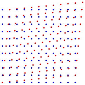
Figure 1: Affine double (pure) shear of two point grids based on (20) for $\varsigma_{1,2}=1$ and $h_{1,2}=a_{0}(n_{1,2}-1)$. Left: $n=121$ points ($n_{1,2}=11$), $a_{0}=1$. Right: $n=441$ points ($n_{1,2}=21$), $a_{0}=\frac{1}{2}$. Blue: initial grid. Red: displaced grid.

From (20) follow $\nabla_{\!\smash{\mathrm{r}}}^{(1)}\bm{\chi}(\bm{x}_{\mathrm{r}})=\bm{I}+(\varsigma_{1}/h_{2})\,\bm{i}_{1}\otimes\bm{i}_{2}+(\varsigma_{2}/h_{1})\,\bm{i}_{2}\otimes\bm{i}_{1}$ and $\nabla_{\!\smash{\mathrm{r}}}^{(d)}\bm{\chi}(\bm{x}_{\mathrm{r}})=\bm{0}$ for $d\geqslant 2$. A fit of $\mathsfbfit{F}_{\!\smash{\beta\pm}}^{(1)}$ to the data in Figure 1 results in fit errors $|\mathsfbfit{F}_{\!\smash{\beta+}}^{(1)}-\nabla_{\!\smash{\mathrm{r}}}^{(1)}\bm{\chi}(\bm{r}_{\beta\mathrm{r}})|$ and $|\mathsfbfit{F}_{\!\smash{\beta-}}^{(1)}-\nabla_{\!\smash{\mathrm{c}}}^{(1)}\bm{\chi}^{-1}(\bm{r}_{\beta\mathrm{c}})|$ of machine precision. In addition, the position ”data” in Figure 1 determine $\mathsfbfit{F}_{\!\smash{\beta\pm}}^{(d)}=\bm{0}$ for $d>1$ to machine precision at all $\beta$. Consequently, determination of $\mathsfbfit{F}_{\!\smash{\beta\pm}}^{(1)}$ recovers the theoretical result independent of resolution in the affine case.

A less trivial case is represented by the non-affine shear

$$\bm{\chi}(\bm{x}_{\mathrm{r}})=\bm{x}_{\mathrm{r}}+\varsigma_{1}f((\bm{i}_{2}\cdot\bm{x}_{\mathrm{r}}-c_{2})/h_{2})\,\bm{i}_{1}\,,\quad f(x):=\frac{\tanh(x)}{2\tanh(c_{2}/h_{2})}\,.$$ (21)

This is displayed for two different values of $h_{2}$ in Figure 2.

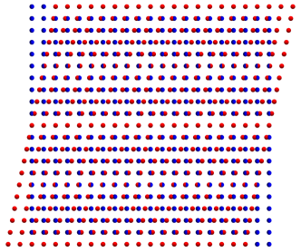
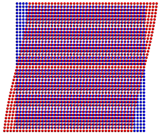
Figure 2: Non-affine shear of two point grids based on (21) for $\varsigma_{1}=2$ and $c_{2}=5$. Left: $n=441$ points ($n_{1,2}=21$), $a_{0}=\frac{1}{2}$, $h_{2}=10$. Right: $n=1681$ points ($n_{1,2}=41$), $a_{0}=\frac{1}{4}$, $h_{2}=5$. Blue: initial grid. Red: displaced grid.

In this case, we have

$$\begin{array}[]{rcl}\nabla_{\!\smash{\mathrm{r}}}^{(1)}\bm{\chi}(\bm{x}_{\mathrm{r}})&=&\bm{I}+(\varsigma_{1}/h_{2})\,f^{\prime}((\bm{i}_{2}\cdot\bm{x}_{\mathrm{r}}-c_{2})/h_{2})\,\bm{i}_{1}\otimes\bm{i}_{2}\,,\\ \nabla_{\!\smash{\mathrm{r}}}^{(2)}\bm{\chi}(\bm{x}_{\mathrm{r}})&=&(\varsigma_{1}/h_{\smash{2}}^{2})\,f^{\prime\prime}((\bm{i}_{2}\cdot\bm{x}_{\mathrm{r}}-c_{2})/h_{2})\,\bm{i}_{1}\otimes\bm{i}_{2}\otimes\bm{i}_{2}\,,\\ \nabla_{\!\smash{\mathrm{r}}}^{(3)}\bm{\chi}(\bm{x}_{\mathrm{r}})&=&(\varsigma_{1}/h_{\smash{2}}^{3})\,f^{\prime\prime\prime}((\bm{i}_{2}\cdot\bm{x}_{\mathrm{r}}-c_{2})/h_{2})\,\bm{i}_{1}\otimes\bm{i}_{2}\otimes\bm{i}_{2}\otimes\bm{i}_{2}\,,\\ &\vdots&\end{array}$$ (22)

from (21), where $\nabla^{(d)}:=\nabla\circ\cdots\circ\nabla$ ($d$ times). As shown in Figure 2, $h_{2}$ controls the ”amount” or ”degree” of non-affinity. Indeed, for ”large” $h_{2}$, $\tanh(x)$ is well-approximated by $\tanh(x)\approx x$, and (21) is nearly affine. As $h_{2}$ decreases, the non-linear terms in $\tanh(x)$ become significant, and the non-affinity of (21) increases.

In the following, results are presented for the accuracy of the largest component of $\mathsfbfit{F}_{\!\smash{\beta+}}^{(d)}$ ($d=1,2,3$) assuming $\varsigma_{1}=2$ and $c_{2}=5$ as in Figure 2. To begin, consider these results for $[\mathsfbfit{F}_{\smash{\beta+}}^{(1)}]_{12}$ with $h_{2}=10$ for two resolutions in Figure 3.

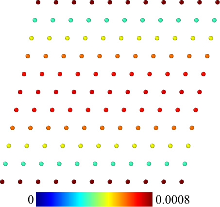
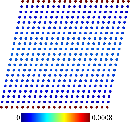
Figure 3: Error $|[\mathsfbfit{F}_{\smash{\beta+}}^{(1)}]_{12}-(\varsigma_{1}/h_{2})\,f^{\prime}((\bm{i}_{2}\cdot\bm{r}_{\smash{\beta\mathrm{r}}}-c_{2})/h_{2})|$ for $h_{2}=10$ and two resolutions.
Left: $a_{0}=1$, $n_{1,2}=11$. Right: $a_{0}=\frac{1}{2}$, $n_{1,2}=21$.

Note that the maximum error of 0.08% is at the upper and lower boundaries of the region normal to the direction $\pm\bm{i}_{2}$ of change in shear. As expected, there is an increase in accuracy with increasing resolution as documented in Figure 3.

These results and trends also hold for increasing non-affinity, as shown by the results in Figure 4 for $h_{2}=5$.

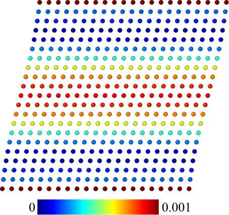
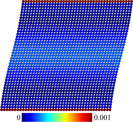
Figure 4: Error $|[\mathsfbfit{F}_{\smash{\beta+}}^{(1)}]_{12}-(\varsigma_{1}/h_{2})\,f^{\prime}((\bm{i}_{2}\cdot\bm{r}_{\smash{\beta\mathrm{r}}}-c_{2})/h_{2})|$ for $h_{2}=5$ and two resolutions.
Left: $a_{0}=\frac{1}{2}$, $n_{1,2}=21$. Right: $a_{0}=\frac{1}{4}$, $n_{1,2}=41$.

Comparison of the results in Figure 4 (left) with those in Figure 3 (right) documents the expected increase in the error of $[\mathsfbfit{F}_{\smash{\beta+}}^{(1)}]_{12}$ as $h_{2}$ decreases (i.e., as the ”amount” of non-affinity increases) at a fixed resolution.

Analogous results for the largest component $[\mathsfbfit{F}_{\smash{\beta+}}^{(2)}]_{122}$ of $\mathsfbfit{F}_{\!\smash{\beta+}}^{(2)}$ are shown in Figure 5 for $h_{2}=10$ and in Figure 6 for $h_{2}=5$ at different resolutions.

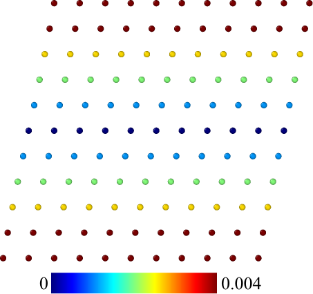
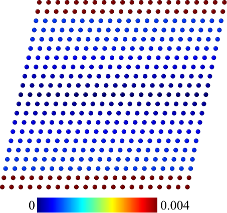
Figure 5: Error $|h_{2}[\mathsfbfit{F}_{\smash{\beta+}}^{(2)}]_{122}-(\varsigma_{1}/h_{2})\,f^{\prime\prime}((\bm{i}_{2}\cdot\bm{r}_{\smash{\beta\mathrm{r}}}-c_{2})/h_{2})|$ for $h_{2}=10$ and two resolutions.
Left: $a_{0}=1$, $n_{1,2}=11$. Right: $a_{0}=\frac{1}{2}$, $n_{1,2}=21$.

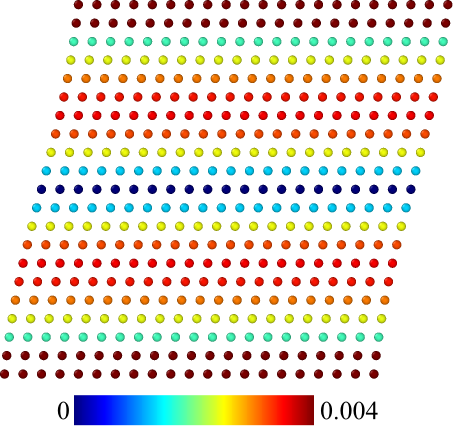
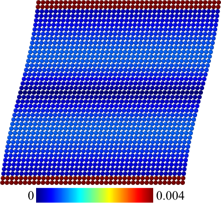
Figure 6: Error $|h_{2}[\mathsfbfit{F}_{\smash{\beta+}}^{(2)}]_{122}-(\varsigma_{1}/h_{2})\,f^{\prime\prime}((\bm{i}_{2}\cdot\bm{r}_{\smash{\beta\mathrm{r}}}-c_{2})/h_{2})|$ for $h_{2}=5$ and two resolutions.
Left: $a_{0}=\frac{1}{2}$, $n_{1,2}=21$. Right: $a_{0}=\frac{1}{4}$, $n_{1,2}=41$.

As in the case of $\mathsfbfit{F}_{\!\smash{\beta+}}^{(1)}$, the maximum error of 0.4% in the largest component $[\mathsfbfit{F}_{\smash{\beta+}}^{(2)}]_{122}$ of $\mathsfbfit{F}_{\!\smash{\beta+}}^{(2)}$ is at the upper and lower boundaries of the region normal to $\bm{i}_{2}$. Since $\mathsfbfit{F}_{\!\smash{\beta+}}^{(1)}$ determines $\mathsfbfit{F}_{\!\smash{\beta+}}^{(2)}$, the corresponding boundary error is in the first two rows of points adjacent to the boundary. In contrast to the results for $[\mathsfbfit{F}_{\smash{\beta+}}^{(1)}]_{12}$, there is no difference in the maximum error of 0.4% between $h_{2}=10$ and $h_{2}=5$.

Lastly, analogous results for the largest component $[\mathsfbfit{F}_{\smash{\beta+}}^{(3)}]_{1222}$ of $\mathsfbfit{F}_{\!\smash{\beta+}}^{(3)}$ are presented in Figure 7 for $h_{2}=10$ and in Figure 8 for $h_{2}=5$ at different resolutions.

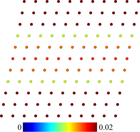
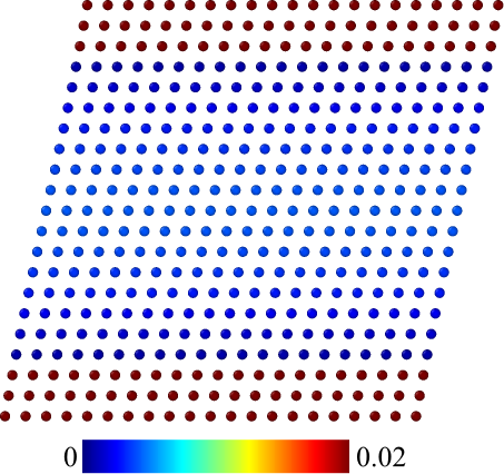
Figure 7: Error $|h_{\smash{2}}^{2}[\mathsfbfit{F}_{\smash{\beta+}}^{(3)}]_{1222}-(\varsigma_{1}/h_{2})\,f^{\prime\prime\prime}((\bm{i}_{2}\cdot\bm{r}_{\smash{\beta\mathrm{r}}}-c_{2})/h_{2})|$ for $h_{2}=10$ and two resolutions.
Left: $a_{0}=1$, $n_{1,2}=11$. Right: $a_{0}=\frac{1}{2}$, $n_{1,2}=21$.

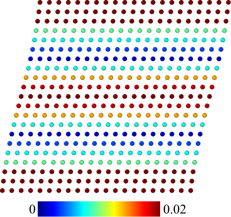
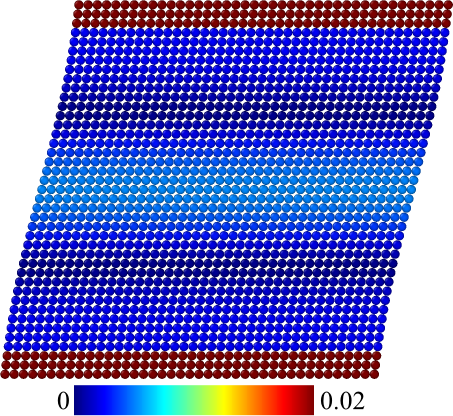
Figure 8: Error $|h_{\smash{2}}^{2}[\mathsfbfit{F}_{\smash{\beta+}}^{(3)}]_{1222}-(\varsigma_{1}/h_{2})\,f^{\prime\prime\prime}((\bm{i}_{2}\cdot\bm{r}_{\smash{\beta\mathrm{r}}}-c_{2})/h_{2})|$ for $h_{2}=5$ and two resolutions.
Left: $a_{0}=\frac{1}{2}$, $n_{1,2}=21$. Right: $a_{0}=\frac{1}{4}$, $n_{1,2}=41$.

As evident, these trends are consistent with those just discussed for $\mathsfbfit{F}_{\!\smash{\beta+}}^{(1)}$ and $\mathsfbfit{F}_{\!\smash{\beta+}}^{(2)}$. As shown by this example, then, discrete local deformation measures of order $2$ and greater characterize the non-affinity of discrete displacement data.

4.2 Displacement of atoms in a dislocated lattice

In this context, the set of points in question are $n$ atoms with positions $\bm{r}_{\!1},\ldots,\bm{r}_{\!n}$ in a crystallographic lattice containing a dislocation. Position results are obtained from molecular statics (MS) simulation of dislocation dipole relaxation. The simulation cells are shown in Figure 9.

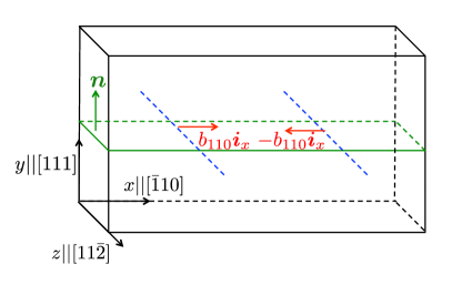
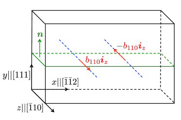
Figure 9: Cells for MS simulation of atomic displacement due to a dissociated dislocation dipole. Initial configuration: perfect dislocations at $(x,y)=(L_{x}/4,L_{y}/2)$ and $(3L_{x}/4,L_{y}/2)$ with Burgers vectors $\pm\bm{b}=\pm a_{0}[\bar{1}10]/2$, $b_{110}=|\bm{b}|=a_{0}/\sqrt{2}$. Left: edge dipole with cell size $(L_{x},L_{y},L_{z})=(120\sqrt{6},180,9\sqrt{2}/2)\,d_{111}$, $d_{111}=a_{0}/\sqrt{3}$. Right: screw dipole with cell size $(L_{x},L_{y},L_{z})=(180\sqrt{2},180,3\sqrt{6})\,d_{111}$. Both cells contain $259200$ atoms.

Rather than Al and Cu as considered by Hartley and Mishin (2005), Au is employed here. Simulations are initialized via conjugate gradient relaxation and quadratic line search under constant (zero) stress and constant (0 K) temperature conditions in LAMMPS Plimpton (1995) via the box/relax command. Initially perfect dipoles are introduced by applying continuum displacements from linear elastic (i.e., Volterra) dislocation theory to core atoms (e.g., Bulatov and Cai, 2006, Chapter 5).Dissociation of these is simulated via 5000 steps of fast inertial relaxation (using FIRE: Bitzek et al., 2006) followed by 5000 steps of conjugate gradient relaxation, at zero stress.

Displacement components for the dissociated left edge monopole in Figure 9 (left) are shown in Figure 10.

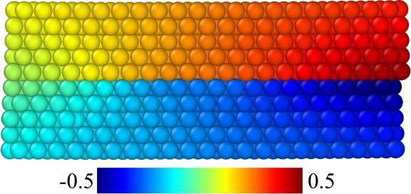
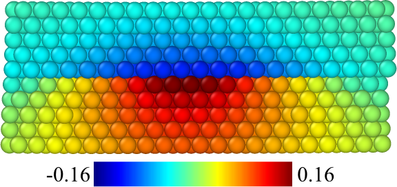
Figure 10: Normalized atomic displacement results $\bm{u}_{\alpha}/|\bm{b}|\cdot\bm{i}_{x}$ (left) and $\bm{u}_{\alpha}/|\bm{b}|\cdot\bm{i}_{z}$ (right) in a region around the dissociated edge monopole at $(x,y)=(L_{x}/4,L_{y}/2)$ in Figure 9 (left) with Burgers vector $\bm{b}=|\bm{b}|\,\bm{i}_{x}=b_{110}\,\bm{i}_{x}$. Regions above and below the glide plane are clearly visible.

Here and in what follows, all results are displayed at atoms in the $(x,y)$ plane perpendicular to the dislocation line, i.e., to $\bm{i}_{z}$. Introducing a straight dislocation with Burgers vector $\bm{b}$ into the bulk lattice on a glide plane results in a displacement $\bm{u}_{\alpha}(t):=\bm{r}_{\!\alpha}(t)-\bm{r}_{\!\alpha}(0)$ of $\alpha=1,\ldots,n$, with $-\frac{1}{2}\leqslant\bm{u}_{\alpha}/|\bm{b}|\cdot\bm{b}/|\bm{b}|\leqslant\frac{1}{2}$. This is shown in Figure 10 (left). The displacement results in Figure 10 determine the position information employed to obtain all discrete local deformation results in the rest of this section.

In contrast to the examples in Section 4.1 for the case of a finite regular grid / simple cubic lattice, all points in an infinite periodic lattice are interior. For atoms with fcc neighborhoods, $r_{\smash{\mathrm{N}s}}=\sqrt{s/2}\,a_{0}$ for $s=1,2,3$, such that $|S_{\!\smash{1\beta}}|=12$, $|S_{\!\smash{2\beta}}|=18$, and $|S_{\!\smash{3\beta}}|=42$. Consequently, $|S_{\!\smash{d\beta}}|>3^{d}$ for $d=1,2,3$. As indicated by the CNA analysis of the dislocated lattice (see Figure 11 below), atoms in the stacking fault (red) have hcp neighborhoods, and those in the partial dislocation cores (white) have triclinic (disordered) neighborhoods; all remaining atoms have fcc neighborhoods. Recall that the cut-off radius $r_{\smash{\mathrm{CNA}}}=\frac{1}{2}(r_{\smash{\mathrm{N}1}}+r_{\smash{\mathrm{N}2}})$ is employed in CNA to determine neighborhoods.

In what follows, $\mathsfbfit{F}_{\!\smash{\beta-}}^{(d)}$ for $d=1,2$ are determined for all atoms based on displacement results in Figure 10. To this end, the algorithm of Hartley and Mishin (2005) is employed. Reduction of $n_{\smash{\beta-}}^{(1)}$ based on their algorithm is shown in Figure 11.

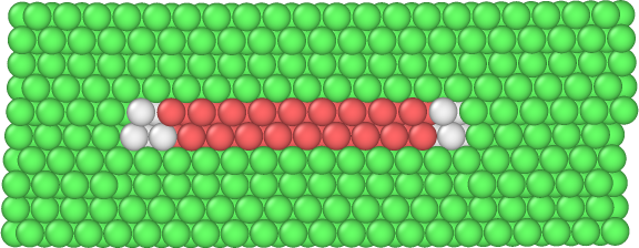
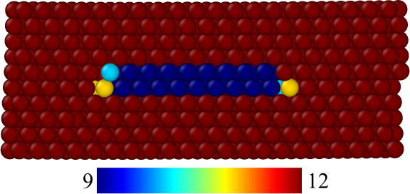
Figure 11: Above: common neighbor analysis (CNA) of atoms in the region around the dissociated edge monopole at $(x,y)=(L_{x}/4,L_{y}/2)$ in Figure 9 (left) showing atoms with lattice (fcc, green), stacking fault (hcp, red), and core (white, disordered) neighborhoods. Below: reduced value of $n_{\smash{\beta-}}^{(1)}$ based on the algorithm of Hartley and Mishin (2005).

Note the reduction of $n_{\smash{\beta-}}^{(1)}$ below (fcc nearest neighbor value) 12 only for atoms in the stacking fault (red) or the partial dislocation cores (white).

4.2.1 Results for edge case

To begin, consider the components of $\mathsfbfit{F}_{\!\smash{\beta-}}^{(1)}$ for the edge case. All results are displayed at atoms in the $(x,y)$ plane perpendicular to the dislocation line, i.e., to $\bm{i}_{z}$, with the Burgers vector in the horizontal $\bm{i}_{x}$ direction. Normal components of this are shown in Figure 12, and shear components in Figure 13.

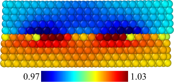
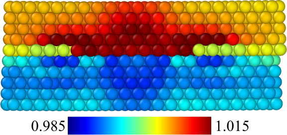
Figure 12: Discrete local deformation of atomic neighborhoods in and around a dissociated edge dislocation core:  $[\mathsfbfit{F}_{\!\smash{\beta-}}^{(1)}]_{xx}$ (left) and $[\mathsfbfit{F}_{\!\smash{\beta-}}^{(1)}]_{yy}$ (right).

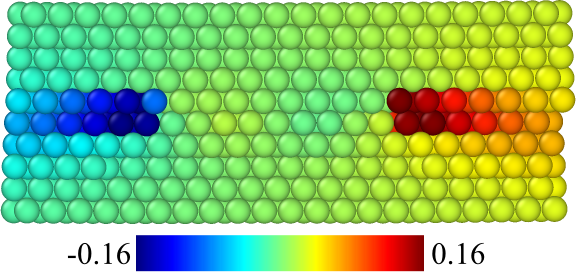
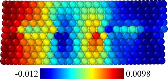
Figure 13: Discrete local deformation of atomic neighborhoods in and around a dissociated edge dislocation core:  $[\mathsfbfit{F}_{\!\smash{\beta-}}^{(1)}]_{xy}$ (left) and $[\mathsfbfit{F}_{\!\smash{\beta-}}^{(1)}]_{yx}$ (right).

Comparison of these results with the CNA-based visualization in Figure 11 (above) shows that maximum normal and shear local deformation (distortion) is associated with the extended defect. Note also that $[\mathsfbfit{F}_{\!\smash{\beta-}}^{(1)}]_{xy}$ in Figure 13 (left) is extremal for the core atoms.

Consider next the largest components of $\mathsfbfit{F}_{\!\smash{\beta-}}^{(2)}$ and $\mathrm{sym}_{2}\mathsfbfit{F}_{\!\smash{\beta-}}^{(2)}$ in Figure 14.

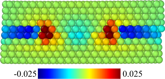
Figure 14: Discrete local deformation of atomic neighborhoods in and around a dissociated edge dislocation core:  $d_{111}[\mathsfbfit{F}_{\!\smash{\beta-}}^{(2)}]_{xyy}$ (left) and $d_{111}[\mathrm{sym}_{2}\mathsfbfit{F}_{\!\smash{\beta-}}^{(2)}]_{xxy}$ (right). Note $d_{111}=a_{0}/\sqrt{3}=2.36\times 10^{-10}$ m for Au with $a_{0}=4.08\times 10^{-10}$ m.

In particular, $[\mathrm{sym}_{2}\mathsfbfit{F}_{\!\smash{\beta-}}^{(2)}]_{xxy}=\tfrac{1}{2}\,[\mathsfbfit{F}_{\!\smash{\beta-}}^{(2)}]_{xxy}+\tfrac{1}{2}\,[\mathsfbfit{F}_{\!\smash{\beta-}}^{(2)}]_{xyx}$. Additional components of $\mathsfbfit{F}_{\!\smash{\beta-}}^{(2)}$ determine the largest components

$$[\mathsfbfit{G}_{\smash{\beta-}}^{(1)}]_{xz}=[\mathsfbfit{F}_{\!\smash{\beta-}}^{(2)}]_{xyz}-[\mathsfbfit{F}_{\!\smash{\beta-}}^{(2)}]_{xxy}\,,\quad[\mathsfbfit{G}_{\smash{\beta-}}^{(1)}]_{zz}=[\mathsfbfit{F}_{\!\smash{\beta-}}^{(2)}]_{zyx}-[\mathsfbfit{F}_{\!\smash{\beta-}}^{(2)}]_{zxy}$$ (23)

of its ”axial vector” $\mathsfbfit{G}_{\smash{\beta-}}^{(1)}:=\mathrm{axv}_{2}\,2\,\mathrm{skw}_{2}\mathsfbfit{F}_{\!\smash{\beta-}}^{(2)}$ via (3) shown in Figure 15.

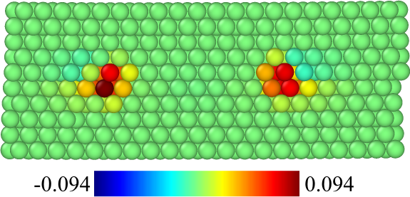
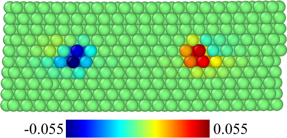
Figure 15: Discrete local deformation of atomic neighborhoods in and around a dissociated edge dislocation core:  $d_{111}[\mathsfbfit{G}_{\smash{\beta-}}^{(1)}]_{xz}$ (left) and $d_{111}[\mathsfbfit{G}_{\smash{\beta-}}^{(1)}]_{zz}$ (right).

Clearly, both $\mathrm{sym}_{2}\mathsfbfit{F}_{\!\smash{\beta-}}^{(2)}$ and $\mathsfbfit{G}_{\smash{\beta-}}^{(1)}$ are non-trivial for atoms in the neighborhood of a dissociated edge monopole in fcc Au.

4.2.2 Results for screw case

Analogous results are obtained for discrete local deformation in atomic neighborhoods in a region surrounding the dissociated screw monopole at $(x,y)=(L_{x}/4,L_{y}/2)$ in Figure 9 (right). Again, all results are displayed at atoms in the $(x,y)$ plane perpendicular to the dislocation line, i.e., to $\bm{i}_{z}$; now, however, the Burgers vector is oriented in the $\bm{i}_{z}$ direction perpendicular to this plane. The largest components of $\mathsfbfit{F}_{\!\smash{\beta-}}^{(1)}$ are shown in Figures 16 and 17.

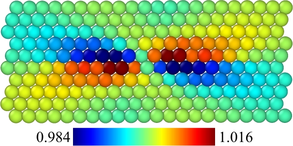
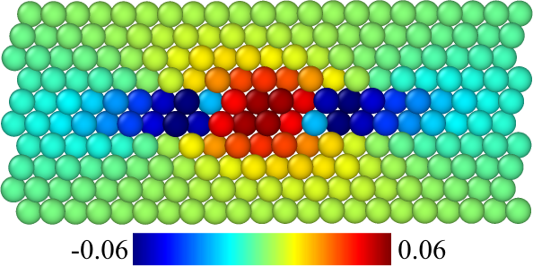
Figure 16: Discrete local deformation of atomic neighborhoods in and around a dissociated screw dislocation core:  $[\mathsfbfit{F}_{\!\smash{\beta-}}^{(1)}]_{xx}$ (left) and $[\mathsfbfit{F}_{\!\smash{\beta-}}^{(1)}]_{xy}$ (right).

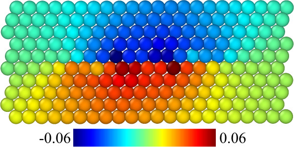
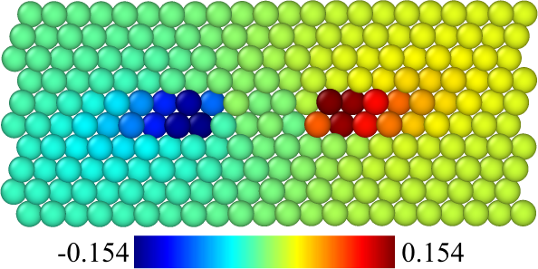
Figure 17: Discrete local deformation of atomic neighborhoods in and around a dissociated screw dislocation core:  $[\mathsfbfit{F}_{\!\smash{\beta-}}^{(1)}]_{zx}$ (left) and $[\mathsfbfit{F}_{\!\smash{\beta-}}^{(1)}]_{zy}$ (right).

Analogous to $[\mathsfbfit{F}_{\!\smash{\beta-}}^{(1)}]_{xy}$ in the edge case in Figure 13 (left), the shear $[\mathsfbfit{F}_{\!\smash{\beta-}}^{(1)}]_{zy}$ in the Burgers vector direction ($\bm{i}_{z}$) perpendicular to the glide plane shown in Figure 17 (right) is the largest component in the screw case as well. Since the dominant partial Burgers vector component is edge-like in Figure 13, and screw-like in Figure 17, note that $[\mathsfbfit{F}_{\!\smash{\beta-}}^{(1)}]_{zy}$ is much more localized to the core atoms than $[\mathsfbfit{F}_{\!\smash{\beta-}}^{(1)}]_{xy}$.

Likewise analogous to the edge case and results for $\mathsfbfit{F}_{\!\smash{\beta-}}^{(2)}$ in Figure 14 are those in Figure 18 for the screw case.

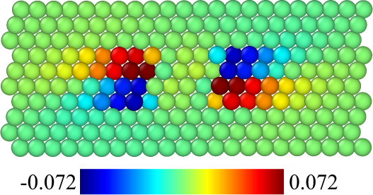
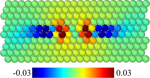
Figure 18: Discrete local deformation of atomic neighborhoods in and around a dissociated screw dislocation core:  $d_{111}[\mathsfbfit{F}_{\!\smash{\beta-}}^{(2)}]_{zyy}$ (left) and $d_{111}[\mathrm{sym}_{2}\mathsfbfit{F}_{\!\smash{\beta-}}^{(2)}]_{zxy}$ (right).

Note that $[\mathrm{sym}_{2}\mathsfbfit{F}_{\!\smash{\beta-}}^{(2)}]_{zxy}=\tfrac{1}{2}\,[\mathsfbfit{F}_{\!\smash{\beta-}}^{(2)}]_{zxy}+\tfrac{1}{2}\,[\mathsfbfit{F}_{\!\smash{\beta-}}^{(2)}]_{zyx}$. Again, since the dominant partial Burgers vector component is edge-like in Figure 14, and screw-like in Figure 18, $[\mathsfbfit{F}_{\!\smash{\beta-}}^{(2)}]_{zyy}$ is much more localized to the core atoms (i.e., partial dislocation lines) than $[\mathsfbfit{F}_{\!\smash{\beta-}}^{(2)}]_{xyy}$. Lastly, Figure 19 displays the largest components of $\mathsfbfit{G}_{\smash{\beta-}}^{(1)}$ for the screw case.

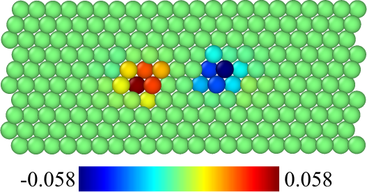
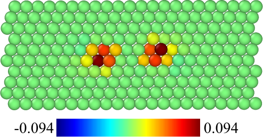
Figure 19: Discrete local deformation of atomic neighborhoods in and around a dissociated screw dislocation core:  $d_{111}[\mathsfbfit{G}_{\smash{\beta-}}^{(1)}]_{xz}$ (left) and $d_{111}[\mathsfbfit{G}_{\smash{\beta-}}^{(1)}]_{zz}$ (right).

These are the same components as those (23) in the edge case. As expected, $[\mathsfbfit{G}_{\smash{\beta-}}^{(1)}]_{xz}>[\mathsfbfit{G}_{\smash{\beta-}}^{(1)}]_{zz}$ in the edge case in Figure 15, and this reverses in the screw case shown in Figure 19. Indeed, $[\mathsfbfit{G}_{\smash{\beta-}}^{(1)}]_{xz}$ is the edge component, and $[\mathsfbfit{G}_{\smash{\beta-}}^{(1)}]_{zz}$ the screw component, of $\mathsfbfit{G}_{\smash{\beta-}}^{(1)}$ for these cases, as we now discuss in more detail.

5 Selected fields determined by discrete local deformation

5.1 Basic considerations

The elements of a discrete local deformation of order $m$ (19) induce a number of different fields. For example, in the simplest case, we have

$$\begin{array}[]{rcl}\bm{\chi}_{\bm{c}}^{\smash{(2)}}(\bm{x})&:=&\bm{\chi}_{\bm{c}}^{\smash{(2)}}(\bm{c})+\mathsfbfit{F}^{(1)}(\bm{x}-\bm{c})+\tfrac{1}{2}\,(\mathsfbfit{F}^{(2)}(\bm{x}-\bm{c}))\,(\bm{x}-\bm{c})\\ \bm{F}_{\!\bm{c}}^{(2)}(\bm{x})&:=&\mathsfbfit{F}^{(1)}+\mathsfbfit{F}^{(2)}(\bm{x}-\bm{c})\,,\end{array}$$ (24)

based on $(\mathsfbfit{F}^{(1)},\mathsfbfit{F}^{(2)})$ and ”centered” at $\bm{c}\in\mathbb{E}^{3}$. Given the identity

$$(\cdots(\mathsfbfit{F}^{(d)}\underbrace{\bm{a})\cdots)\,\bm{a}}\nolimits_{k\ \mathrm{times}}=(\cdots((\mathrm{sym}_{k}\mathsfbfit{F}^{(d)})\underbrace{\bm{a})\cdots)\,\bm{a}}\nolimits_{k\ \mathrm{times}}\,,\ \ k\leqslant d\,,$$ (25)

based on (1), one sees that (24)₁ depends in fact only on the completely symmetric part $\mathrm{sym}_{2}\mathsfbfit{F}^{(2)}$ of $\mathsfbfit{F}^{(2)}$, i.e.,

$$\bm{\chi}_{\bm{c}}^{\smash{(2)}}(\bm{x})=\bm{\chi}_{\bm{c}}^{\smash{(2)}}(\bm{c})+\mathsfbfit{F}^{(1)}(\bm{x}-\bm{c})+\tfrac{1}{2}\,((\mathrm{sym}_{2}\mathsfbfit{F}^{(2)})\,(\bm{x}-\bm{c}))\,(\bm{x}-\bm{c})\,.$$ (26)

In this case, the difference

$$\begin{array}[]{rcl}\bm{F}_{\!\bm{c}}^{(2)}(\bm{x})-\nabla\bm{\chi}_{\bm{c}}^{\smash{(2)}}(\bm{x})&=&(\mathrm{skw}_{2}\mathsfbfit{F}^{(2)})\,(\bm{x}-\bm{c})\end{array}$$ (27)

is determined by the completely skew-symmetric part $\mathrm{skw}_{2}\mathsfbfit{F}^{(2)}$ of $\mathsfbfit{F}^{(2)}$. In addition,

$$\begin{array}[]{rclcl}\mathop{\mathrm{curl}}\nabla\bm{\chi}_{\bm{c}}^{\smash{(2)}}&=&\mathrm{axv}_{\mathrm{2}}\,2\,\mathrm{skw}_{2}\,\mathrm{sym}_{2}\mathsfbfit{F}^{(2)}&=&\bm{0}\,,\\ \mathop{\mathrm{curl}}\bm{F}_{\!\bm{c}}^{(2)}&=&\mathrm{axv}_{\mathrm{2}}\,2\,\mathrm{skw}_{2}\mathsfbfit{F}^{(2)}&\neq&\bm{0}\,,\end{array}$$ (28)

hold via (2)₂, (3) and (A.4).

Examples of (24)₂ include those

$$\bm{F}_{\!\smash{\beta\mathrm{r}}}(\bm{x}_{\mathrm{r}}):=\mathsfbfit{F}_{\smash{\beta+}}^{(1)}+\mathsfbfit{F}_{\smash{\beta+}}^{(2)}(\bm{x}_{\mathrm{r}}-\bm{r}_{\!\smash{\beta\mathrm{r}}})\,,\quad\bm{F}_{\!\smash{\beta\mathrm{c}}}^{-1}(\bm{x}_{\mathrm{c}}):=\mathsfbfit{F}_{\smash{\beta-}}^{(1)}+\mathsfbfit{F}_{\smash{\beta-}}^{(2)}(\bm{x}_{\mathrm{c}}-\bm{r}_{\!\smash{\beta\mathrm{c}}})\,,$$ (29)

determined by $(\mathsfbfit{F}_{\smash{\beta\pm}}^{(1)},\mathsfbfit{F}_{\smash{\beta\pm}}^{(2)})$ from Section 4. In this context, we have

$$\begin{array}[]{rclcl}\mathrm{curl}_{\mathrm{r}}\bm{F}_{\!\beta\mathrm{r}}&=&\mathrm{axv}_{\mathrm{2}\,}2\,\mathrm{skw}_{2}\mathsfbfit{F}_{\!\smash{\beta+}}^{(2)}&=:&\mathsfbfit{G}_{\smash{\beta+}}^{(1)}\,,\\ \mathrm{curl}_{\mathrm{c}}\bm{F}_{\!\smash{\beta\mathrm{c}}}^{-1}&=&\mathrm{axv}_{\mathrm{2}\,}2\,\mathrm{skw}_{2}\mathsfbfit{F}_{\!\smash{\beta-}}^{(2)}&=:&\mathsfbfit{G}_{\smash{\beta-}}^{(1)}\,.\end{array}$$ (30)

In particular, note the formal analogy of $\mathrm{curl}_{\mathrm{c}}\bm{F}_{\!\smash{\beta\mathrm{c}}}^{-1}$ to $\mathrm{curl}_{\mathrm{c}}\bm{F}_{\!\smash{\mathrm{L}}}^{-1}$ in the context of the multiplicative decompostion $\nabla\bm{\chi}=\bm{F}_{\!\mathrm{L}}\bm{F}_{\!\mathrm{R}}$ of the continuum deformation gradient into lattice $\bm{F}_{\!\mathrm{L}}$ and residual (e.g., dislocation) $\bm{F}_{\!\mathrm{R}}$ contributions. As well known in continuum dislocation theory (e.g., Cermelli and Gurtin, 2001), $\mathrm{curl}_{\mathrm{c}}\bm{F}_{\!\smash{\mathrm{L}}}^{-1}$ is a finite deformation generalization of the Nye dislocation tensor Nye (1953).

Consider next the fields

$$\begin{array}[]{rcl}\bm{\chi}_{\bm{c}}^{\smash{(3)}}(\bm{x})&:=&\bm{\chi}_{\bm{c}}^{\smash{(3)}}(\bm{c})+\mathsfbfit{F}^{(1)}(\bm{x}-\bm{c})+\tfrac{1}{2}\,((\mathrm{sym}_{2}\mathsfbfit{F}^{(2)})\,(\bm{x}-\bm{c}))\,(\bm{x}-\bm{c})\\ &+&\tfrac{1}{3}\,(((\mathrm{sym}_{3}\mathsfbfit{F}^{(3)})\,(\bm{x}-\bm{c}))\,(\bm{x}-\bm{c}))\,(\bm{x}-\bm{c})\,,\\ \bm{F}_{\!\bm{c}}^{(3)}(\bm{x})&:=&\mathsfbfit{F}^{(1)}+\mathsfbfit{F}^{(2)}(\bm{x}-\bm{c})+((\mathrm{sym}_{2}\mathsfbfit{F}^{(3)})\,(\bm{x}-\bm{c}))\,(\bm{x}-\bm{c})\,,\end{array}$$ (31)

centered at $\bm{c}$ and determined by $(\mathsfbfit{F}^{(1)},\mathsfbfit{F}^{(2)},\mathsfbfit{F}^{(3)})$ via (25). In this case,

$$\begin{array}[]{rclcl}\mathop{\mathrm{curl}}\nabla\bm{\chi}_{\bm{c}}^{\smash{(3)}}&=&\mathrm{axv}_{\mathrm{2}}\,2\,\mathrm{skw}_{2}\,[\mathrm{sym}_{2}\mathsfbfit{F}^{(2)}+2\,(\mathrm{sym}_{3}\mathsfbfit{F}^{(3)})\,(\bm{x}-\bm{c})]&=&\bm{0}\,,\\ \mathop{\mathrm{curl}}\bm{F}_{\!\bm{c}}^{(3)}&=&\mathrm{axv}_{\mathrm{2}}\,2\,\mathrm{skw}_{2}\,[\mathsfbfit{F}^{(2)}+2\,(\mathrm{sym}_{2}\mathsfbfit{F}^{(3)})\,(\bm{x}-\bm{c})]&\neq&\bm{0}\,,\end{array}$$ (32)

hold analogous to (28). Further,

$$\bm{F}_{\!\bm{c}}^{(3)}(\bm{x})-\nabla\bm{\chi}_{\bm{c}}^{\smash{(3)}}(\bm{x})=(\mathrm{skw}_{2}\mathsfbfit{F}^{(2)})\,(\bm{x}-\bm{c})+((\mathrm{sym}_{2,3}\mathsfbfit{F}^{(3)})\,(\bm{x}-\bm{c}))\,(\bm{x}-\bm{c})$$ (33)

is determined not only by $\mathrm{skw}_{2}\mathsfbfit{F}^{(2)}$ as in (27) above, but also by the difference

$$\mathrm{sym}_{d-1,d}\mathsfbfit{F}^{(d)}:=\mathrm{sym}_{d-1}\mathsfbfit{F}^{(d)}-\mathrm{sym}_{d}\mathsfbfit{F}^{(d)}$$ (34)

for $d=3$. This is also true for the general deformation fields

$$\begin{array}[]{rcl}\bm{\chi}_{\bm{c}}^{\smash{(m)}}(\bm{x})&=&\bm{\chi}_{\!\bm{c}}^{\smash{(m)}}(\bm{c})+\mathsfbfit{F}^{(1)}(\bm{x}-\bm{c})+\tfrac{1}{2}\,((\mathrm{sym}_{2}\mathsfbfit{F}^{(2)})\,(\bm{x}-\bm{c}))\,(\bm{x}-\bm{c})+\cdots\\ &+&\tfrac{1}{m}\,(\cdots((\mathrm{sym}_{m}\mathsfbfit{F}^{(m)})\underbrace{(\bm{x}-\bm{c}))\cdots)\,(\bm{x}-\bm{c})}\nolimits_{m\,\mathrm{times}}\,,\\ \bm{F}_{\!\bm{c}}^{(m)}(\bm{x})&:=&\mathsfbfit{F}^{(1)}+\mathsfbfit{F}^{(2)}(\bm{x}-\bm{c})+((\mathrm{sym}_{2}\mathsfbfit{F}^{(3)})\,(\bm{x}-\bm{c}))\,(\bm{x}-\bm{c})+\cdots\\ &+&(\cdots((\mathrm{sym}_{m-1}\mathsfbfit{F}^{(m)})\underbrace{(\bm{x}-\bm{c}))\cdots)\,(\bm{x}-\bm{c})}\nolimits_{(m-1)\,\mathrm{times}}\,,\end{array}$$ (35)

induced by all elements of (19), i.e.,

$$\begin{array}[]{rcl}\bm{F}_{\!\bm{c}}^{(m)}-\nabla\bm{\chi}_{\!\bm{c}}^{\smash{(m)}}(\bm{x})&=&(\mathrm{skw}_{2}\mathsfbfit{F}^{(2)})\,(\bm{x}-\bm{c})+((\mathrm{sym}_{2,3}\mathsfbfit{F}^{(3)})\,(\bm{x}-\bm{c}))\,(\bm{x}-\bm{c})+\cdots\\ &+&(\cdots((\mathrm{sym}_{m-1,m}\mathsfbfit{F}^{(m)})\underbrace{(\bm{x}-\bm{c}))\cdots)\,(\bm{x}-\bm{c})}\nolimits_{(m-1)\,\mathrm{times}}\,.\end{array}$$ (36)

Like in the case of $\bm{\chi}_{\bm{c}}^{\smash{(2,3)}}$ discussed above, $\mathop{\mathrm{curl}}\nabla\bm{\chi}_{\bm{c}}^{\smash{(m)}}=\bm{0}$, again via (25). Besides the difference between the two measures, the right-hand sides of (27), (33) and (36) represent the information contained in (19) which is lost when one works with $\bm{\chi}_{\bm{c}}^{\smash{(m)}}$ alone.

5.2 Generalization of local subset DIC

In the current notation, local subset DIC is based on the model form

$$\textstyle\bm{\chi}_{\mathrm{DIC}}(\bm{x}_{\mathrm{r}}):=\sum_{i}\kappa_{i}(\bm{x}_{\mathrm{r}})\,\bm{\chi}_{\smash{\bm{x}_{i\mathrm{r}}}}^{(1)}(\bm{x}_{\mathrm{r}})\,,$$ (37)

for the continuum deformation field of a region of interest $R=\bigcup_{i}R_{i}$, with

$$\bm{\chi}_{\smash{\bm{x}_{i\mathrm{r}}}}^{(1)}(\bm{x}_{\mathrm{r}}):=\bm{\chi}_{\smash{\bm{x}_{i\mathrm{r}}}}^{(1)}(\bm{x}_{i\mathrm{r}})+\mathsfbfit{F}_{\smash{i+}}^{(1)}(\bm{x}_{\mathrm{r}}-\bm{x}_{i\mathrm{r}})\,,\quad\bm{x}_{i\mathrm{c}}=\bm{\chi}_{\smash{\bm{x}_{i\mathrm{r}}}}^{\smash{(1)}}(\bm{x}_{i\mathrm{r}})\,.$$ (38)

Assume now that $(\mathsfbfit{F}_{\!\smash{i+}}^{(1)},\ldots,\mathsfbfit{F}_{\!\smash{i+}}^{(m)})$ has been determined for each $R_{i}\subset R$. In this case, (37) generalizes directly to

$$\textstyle\bm{\chi}_{\mathrm{DIC}}(\bm{x}_{\mathrm{r}}):=\sum_{i}\kappa_{i}(\bm{x}_{\mathrm{r}})\,\bm{\chi}_{\!\smash{\bm{x}_{i\mathrm{r}}}}^{(m)}(\bm{x}_{\mathrm{r}})$$ (39)

via (35)₁. In addition, local subset DIC can be generalized to the determination of

$$\textstyle\bm{F}_{\mathrm{DIC}}(\bm{x}_{\mathrm{r}}):=\sum_{i}\kappa_{i}(\bm{x}_{\mathrm{r}})\,\bm{F}_{\!\smash{\bm{x}_{i\mathrm{r}}}}^{(m)}(\bm{x}_{\mathrm{r}})$$ (40)

as well via (35)₂. Besides being of interest in its own right, extending or generalizing local subset DIC in this fashion accounts for the additional physical information contained in $(\mathsfbfit{F}_{\!\smash{i+}}^{(1)},\ldots,\mathsfbfit{F}_{\!\smash{i+}}^{(m)})$ on generally non-affine and / or incompatible local deformation in real materials.

6 Relation of current treatment to selected previous work

Besides to Hartley and Mishin (2005) and Shimizu et al. (2007), the current treatment is most closely related to that of Zimmerman et al. (2009). In particular, these latter authors work with the generalization

$$\bm{s}_{\alpha\beta}(t)\approx\mathsfbfit{F}_{\!\smash{\beta+}}^{(1)}(t)\,\bm{s}_{\alpha\beta}(0)+\tfrac{1}{2}\,(\mathsfbfit{S}_{\smash{\beta+}}^{(2)}(t)\,\bm{s}_{\alpha\beta}(0))\,\bm{s}_{\alpha\beta}(0)$$ (41)

of the first-order case (4)₁ (i.e., their Equation (18)), where $\mathsfbfit{S}_{\smash{\beta+}}^{(2)}(t)\in\mathrm{Sym}_{2,2}(\mathbb{V}^{3},\mathbb{V}^{3})$. In addition, note that their Equation (40) corresponds to (10)₁ for $\mathsfbfit{F}_{\!\smash{\beta+}}^{(2)}$. These authors do not consider $\mathsfbfit{F}_{\!\smash{\beta-}}^{(1)}$ from (4)₂ and $\mathsfbfit{F}_{\!\smash{\beta-}}^{(2)}$ from (10)₂. As mentioned above, the first of these was treated by Hartley and Mishin (2005).

Although somewhat different in purpose, the more recent work of Zhang et al. (2015) is conceptually related to the current treatment as well. These authors employ a weighted least-squares fit of

$$\begin{array}[]{rclcl}\bm{r}_{\!\alpha}(t)&\approx&\bm{\chi}_{\mathrm{Z}t}(\bm{r}_{\!\alpha}(0))&=&\bm{\chi}_{\mathrm{Z}t}(\bm{x}_{\mathrm{r}}+\bm{s}_{\alpha}(0))\\ &&&\approx&\bm{\chi}_{\mathrm{Z}t}(\bm{x}_{\mathrm{r}})+\nabla_{\!\smash{\mathrm{r}}}^{(1)}\bm{\chi}_{\mathrm{Z}t}(\bm{x}_{\mathrm{r}})\,\bm{s}_{\alpha}(0)+\tfrac{1}{2!}\,(\nabla_{\!\smash{\mathrm{r}}}^{(2)}\bm{\chi}_{\mathrm{Z}t}(\bm{x}_{\mathrm{r}})\,\bm{s}_{\alpha}(0))\bm{s}_{\alpha}(0)\end{array}$$ (42)

(based on their Equations (12)-(20) and (33)-(43)) to atomic position results $\bm{r}_{\!\alpha}$, $\alpha=1,\ldots,n$, from molecular dynamics (MD) at the position $\bm{x}_{\mathrm{r}}\in B_{\mathrm{r}}$ in a reference configuration $B_{\mathrm{r}}\subset\mathbb{E}^{3}$. In the process, best-fit values of

$$\bm{x}_{\mathrm{c}}=\bm{\chi}_{\mathrm{Z}t}(\bm{x}_{\mathrm{r}})\in\mathbb{V}^{3}\,,\ \ \nabla_{\!\smash{\mathrm{r}}}^{(1)}\bm{\chi}_{\mathrm{Z}t}(\bm{x}_{\mathrm{r}})\in\mathrm{Lin}_{1}(\mathbb{V}^{3},\mathbb{V}^{3})\,,\ \ \nabla_{\!\smash{\mathrm{r}}}^{(2)}\bm{\chi}_{\mathrm{Z}t}(\bm{x}_{\mathrm{r}})\in\mathrm{Sym}_{2,2}(\mathbb{V}^{3},\mathbb{V}^{3})\,,$$ (43)

are determined for all atoms (i.e., in the simulation cell) at $\bm{x}_{\mathrm{r}}\in B_{\mathrm{r}}$.

As implied by the dislocation core example in Section 4.2, even for the displacement of atoms in the neighborhood of a single atom located at $\bm{r}_{\beta}(0)=\bm{x}_{\mathrm{r}}$, both (41) and (42) may be qualitatively too special. Indeed, in contrast to the analogous discrete local deformation $(\mathsfbfit{F}_{\!\smash{\beta+}}^{(1)}(t),\mathsfbfit{F}_{\!\smash{\beta+}}^{(2)}(t))$, neither $\mathsfbfit{S}_{\smash{\beta+}}^{(2)}(t)$ nor $\nabla_{\!\smash{\mathrm{r}}}^{(2)}\bm{\chi}_{\mathrm{Z}t}(\bm{x}_{\mathrm{r}})$ captures any incompatible contribution from these displacements to continuum (local) deformation. Moreover, it is not clear that it makes physical sense in general to assume that there exists a single continuum deformation field $\bm{\chi}_{\mathrm{Z}t}$ which represents the displacements of all atoms at any $\bm{x}_{\mathrm{r}}\in B_{\mathrm{r}}$. Indeed, any deformation field like $\bm{\chi}_{\mathrm{Z}t}$ is in fact just one element of an equivalence class $[\bm{\chi}]_{\smash{\bm{x}_{\mathrm{r}}}}^{(2)}$ of such fields at any $\bm{x}_{\mathrm{r}}\in B_{\mathrm{r}}$; for the case of order $m$, $[\bm{\chi}]_{\smash{\bm{x}_{\mathrm{r}}}}^{(m)}$ is defined by

$$\nabla_{\!\smash{\mathrm{r}}}^{(1)}\bm{\chi}_{a}(\bm{x}_{\mathrm{r}})=\nabla_{\!\smash{\mathrm{r}}}^{(1)}\bm{\chi}_{b}(\bm{x}_{\mathrm{r}})\,,\ldots,\nabla_{\!\smash{\mathrm{r}}}^{(m)}\bm{\chi}_{a}(\bm{x}_{\mathrm{r}})=\nabla_{\!\smash{\mathrm{r}}}^{(m)}\bm{\chi}_{b}(\bm{x}_{\mathrm{r}})\,,$$ (44)

for all $\bm{\chi}_{a},\bm{\chi}_{b}\in[\bm{\chi}]_{\smash{\bm{x}_{\mathrm{r}}}}^{(m)}$. Likewise,

$$\nabla_{\!\smash{\mathrm{c}}}^{(1)}\bm{\chi}_{a}^{\smash{-1}}(\bm{x}_{\mathrm{c}})=\nabla_{\!\smash{\mathrm{c}}}^{(1)}\bm{\chi}_{b}^{\smash{-1}}(\bm{x}_{\mathrm{c}})\,,\ldots,\nabla_{\!\smash{\mathrm{c}}}^{(m)}\bm{\chi}_{a}^{\smash{-1}}(\bm{x}_{\mathrm{c}})=\nabla_{\!\smash{\mathrm{c}}}^{(m)}\bm{\chi}_{b}^{\smash{-1}}(\bm{x}_{\mathrm{c}})\,,$$ (45)

for all $\bm{\chi}_{a}^{\smash{-1}},\bm{\chi}_{b}^{\smash{-1}}\in[\bm{\chi}^{\smash{-1}}]_{\smash{\bm{x}_{\mathrm{c}}}}^{(m)}$ defines the equivalence class $[\bm{\chi}^{\smash{-1}}]_{\smash{\bm{x}_{\mathrm{c}}}}^{(m)}$ at any position $\bm{x}_{\mathrm{c}}\in B_{\mathrm{c}}$ in the current configuration $B_{\mathrm{c}}\subset\mathbb{E}^{3}$. Since $\nabla_{\!\smash{\mathrm{r}}}^{(d)}\bm{\chi}(\bm{x}_{\mathrm{r}})\in\mathrm{Sym}_{d,d}(\mathbb{V}^{3},\mathbb{V}^{3})$, note that the completely symmetric part $(\mathsfbfit{F}_{+}^{\smash{(1)}},\mathrm{sym}_{2}\mathsfbfit{F}_{+}^{\smash{(2)}},\ldots,\mathrm{sym}_{m}\mathsfbfit{F}_{+}^{\smash{(m)}})$ of the discrete local deformation $(\mathsfbfit{F}_{+}^{\smash{(1)}},\mathsfbfit{F}_{+}^{\smash{(2)}},\ldots,\mathsfbfit{F}_{+}^{\smash{(m)}})$ can represent $[\bm{\chi}]_{\smash{\bm{x}_{\mathrm{r}}}}^{(m)}$. Similarly, $[\bm{\chi}^{-1}]_{\smash{\bm{x}_{\mathrm{c}}}}^{(m)}$ can be represented by the completely symmetric part $(\mathsfbfit{F}_{-}^{\smash{(1)}},\mathrm{sym}_{2}\mathsfbfit{F}_{-}^{\smash{(2)}},\ldots,\mathrm{sym}_{m}\mathsfbfit{F}_{-}^{\smash{(m)}})$ of $(\mathsfbfit{F}_{-}^{\smash{(1)}},\mathsfbfit{F}_{-}^{\smash{(2)}},\ldots,\mathsfbfit{F}_{-}^{\smash{(m)}})$.

7 Summary and discussion

In the current work, the concept of discrete local deformation of order $m$ has been developed to characterize discrete displacement data in a pseudo-continuum kinematic fashion. Central to the current approach are the generalizations (10) and (14) of (4). Together with (4), these result in a hierarchical determination of discrete local deformation from discrete position information in the sense that order $m$ depends on the results of all lower orders $m-1,\ldots,1$. The least-squares-based over-determination of discrete local deformation measures gives these the character of spatially-averaged quantities in a (finite) neighborhood of each point. The current approach generalizes those of Hartley and Mishin (2005), Shimizu et al. (2007) and Zimmerman et al. (2009) for the determination of order $m=1$ discrete local deformation from atomic displacement information to (i) arbitrary discrete displacement information and (ii) discrete local deformation measures of order $m>2$. More specifically, Shimizu et al. (2007) worked explicitly with (7)₁ based on (4)₁, and Hartley and Mishin (2005) with (7)₂ based on (4)₂. In addition, Zimmerman et al. (2009) discussed relations equivalent to (13)₁ based on (10)₁.

As implied by the results in Section 4.1, for a region of fixed spatial size (i.e., specimen size, simulation cell size), the determination of $\mathsfbfit{F}_{\!\smash{\beta\pm}}^{(d)}$ for $d=1,\ldots,m$ is influenced by the point spacing / number $n$ of points. In the experimental context, this spacing is limited by the resolution of the measurement method (e.g., local subset DIC). In the lattice / atomistic context (e.g., Section 4.2), this spacing is atomic and so (physically) fixed. In both cases, the size of $n_{\smash{\beta}}^{(d)}<n$ is also relevant. Since this is not known a-priori (especially in the empirical, experimental context), a convergence study is indicated, formally analogous to that in the numerical solution of continuum boundary-value problems.

In the approach developed in Section 3, the discrete local deformation measures $\mathsfbfit{F}_{\!\smash{\beta\pm}}^{(1)},\ldots,\mathsfbfit{F}_{\!\smash{\beta\pm}}^{(m)}$ are determined from $\bm{r}_{\!1},\ldots,\bm{r}_{\!n}$ in a completely ”decoupled” fashion, representing the simplest approach. A more accurate, coupled determination, however, is also possible. For example, consider the ”first-order” generalizations

$$\begin{array}[]{rcl}\bm{s}_{\alpha\beta\pm}&\approx&\mathsfbfit{F}_{\!\smash{\beta\pm}}^{(1)}\,\bm{s}_{\alpha\beta\pm}+\tfrac{1}{2}\,((\mathrm{sym}_{2}\mathsfbfit{F}_{\smash{\beta\pm}}^{(2)})\,\bm{s}_{\alpha\beta\pm})\,\bm{s}_{\alpha\beta\pm}\,,\\ \mathsfbfit{F}_{\smash{\alpha\pm}}^{(1)}&\approx&\mathsfbfit{F}_{\smash{\beta\pm}}^{(1)}+\mathsfbfit{F}_{\smash{\beta\pm}}^{(2)}\,\bm{s}_{\alpha\beta\pm}\,,\end{array}$$ (46)

of (4) and (10) via (9) with $\bm{s}_{\alpha\beta-}:=\bm{s}_{\alpha\beta}(t)$ and $\bm{s}_{\alpha\beta+}:=\bm{s}_{\alpha\beta}(0)$ for simultaneous determination of $\mathsfbfit{F}_{\!\smash{\beta\pm}}^{(1)}$ and $\mathsfbfit{F}_{\!\smash{\beta\pm}}^{(2)}$ for $\beta=1,\ldots,n$. The Euler-Lagrange relations of the corresponding generalization

$$\begin{array}[]{l}f(\mathsfbfit{F}_{\!\smash{1\pm}}^{(1)},\ldots,\mathsfbfit{F}_{\!\smash{n\pm}}^{(1)},\mathsfbfit{F}_{\!\smash{1\pm}}^{(2)},\ldots,\mathsfbfit{F}_{\!\smash{n\pm}}^{(2)})\\ \quad=\ \frac{1}{2}\sum_{\beta=1}^{n}\sum_{\alpha=1_{\beta\pm}}^{n_{\beta\pm}}|\bm{s}_{\alpha\beta\pm}-\mathsfbfit{F}_{\!\smash{\beta\pm}}^{(1)}\bm{s}_{\alpha\beta\mp}-\tfrac{1}{2}\,(\mathsfbfit{F}_{\smash{\beta\pm}}^{(2)}\bm{s}_{\alpha\beta\mp})\,\bm{s}_{\alpha\beta\mp}|^{2}\\ \quad+\ \ \frac{1}{2}\sum_{\beta=1}^{n}\sum_{\alpha=1_{\beta\pm}}^{n_{\beta\pm}}|\mathsfbfit{F}_{\smash{\alpha\pm}}^{(1)}-\mathsfbfit{F}_{\smash{\beta\pm}}^{(1)}-\mathsfbfit{F}_{\smash{\beta\pm}}^{(2)}\bm{s}_{\alpha\beta\mp}|^{2}\,,\end{array}$$ (47)

of the least-squares-based objective function with $n_{\beta\pm}:=n_{\smash{\beta\pm}}^{(1,2)}$ yield a couple system for $\mathsfbfit{F}_{\!\smash{1\pm}}^{(1)},\ldots,\mathsfbfit{F}_{\!\smash{n\pm}}^{(1)},\mathsfbfit{F}_{\!\smash{1\pm}}^{(2)},\ldots,\mathsfbfit{F}_{\!\smash{n\pm}}^{(2)}$ which can be solved numerically. Starting values for the corresponding iterative solution are available from the decoupled determination of these developed in Section 3.

The concept of discrete local deformation employed here as based on can be developed further in a number of directions. For example, note that (19) can be expressed in the ”reduced” form

$$(\mathsfbfit{F}^{(1)},\mathsfbfit{\Gamma}^{(2)},\ldots,\mathsfbfit{\Gamma}^{(m)})\,,\quad\mathsfbfit{\Gamma}^{(d)}:=\mathsfbfit{F}^{(1)\,-1}\mathsfbfit{F}^{(d)}\,.$$ (48)

In the context of Section 3, for example, note that $\mathsfbfit{F}_{\!\smash{\beta\pm}}^{(1)}$ and $\mathsfbfit{F}_{\!\smash{\beta\pm}}^{(d)}$ determine $\mathsfbfit{\Gamma}_{\!\smash{\beta\pm}}^{(d)}$ for $d=2,\ldots,m$ via (48). Referring again to the discrete position configuration $\bm{r}_{\!1}(t),\ldots,\bm{r}_{\!n}(t)$ as current, and to $\bm{r}_{\!1}(0),\ldots,\bm{r}_{\!n}(0)$ as referential, note that the discrete local deformation measures $\mathsfbfit{F}_{\!\smash{\beta\pm}}^{(d)}$ are mixed current-referential, whereas $\mathsfbfit{\Gamma}_{\!\smash{\beta+}}^{(d)}$ is purely referential, and $\mathsfbfit{\Gamma}_{\!\smash{\beta-}}^{(d)}$ purely current, in character. This is also the case for the corresponding fields. Local deformation fields induced by (48) include those

$$\begin{array}[]{rcl}\bm{D}_{\!\bm{c}}^{(2)}(\bm{x})&:=&\mathsfbfit{I}^{(1)}+\mathsfbfit{\Gamma}^{(2)}(\bm{x}-\bm{c})\,,\\ \bm{D}_{\!\bm{c}}^{(d)}(\bm{x})&:=&\mathsfbfit{I}^{(1)}+\mathsfbfit{\Gamma}^{(2)}(\bm{x}-\bm{c})+((\mathrm{sym}_{2}\mathsfbfit{\Gamma}^{(3)})\,(\bm{x}-\bm{c}))\,(\bm{x}-\bm{c})+\cdots\\ &+&(\cdots((\mathrm{sym}_{d-1}\mathsfbfit{\Gamma}^{(d)})\underbrace{(\bm{x}-\bm{c}))\cdots)\,(\bm{x}-\bm{c})}\nolimits_{(d-1)\,\mathrm{times}}\,,\end{array}$$ (49)

for $3\leqslant d\leqslant m$. Analogous to (29), for example,

$$\bm{D}_{\beta\mathrm{r}}(\bm{x}_{\mathrm{r}}):=\bm{I}+\mathsfbfit{\Gamma}_{\!\smash{\beta+}\,}^{(2)}(\bm{x}_{\mathrm{r}}-\bm{r}_{\!\smash{\beta\mathrm{r}}})\,,\quad\bm{D}_{\smash{\beta\mathrm{c}}}^{(2)}(\bm{x}_{\mathrm{c}}):=\bm{I}+\mathsfbfit{\Gamma}_{\!\smash{\beta-}\,}^{(2)}(\bm{x}_{\mathrm{c}}-\bm{r}_{\!\smash{\beta\mathrm{c}}})\,,$$ (50)

are purely referential, and purely current, respectively, in character, in contrast to the mixed current-referential measures $\bm{F}_{\!\beta\mathrm{r}}$ and $\bm{F}_{\!\smash{\beta\mathrm{c}}}^{-1}$. Likewise, whereas $\mathrm{curl}_{\mathrm{r}}\bm{F}_{\!\beta\mathrm{r}}=\mathsfbfit{F}_{\!\smash{\beta+}}^{(1)}\,\mathrm{curl}_{\mathrm{r}}\bm{D}_{\beta\mathrm{r}}$ and $\mathrm{curl}_{\mathrm{c}}\bm{F}_{\!\smash{\beta\mathrm{c}}}^{-1}=\mathsfbfit{F}_{\!\smash{\beta-}}^{(1)}\,\mathrm{curl}_{\mathrm{c}}\bm{D}_{\smash{\beta\mathrm{c}}}$ are mixed, $\mathrm{curl}_{\mathrm{r}}\bm{D}_{\!\beta\mathrm{r}}$ is purely referential, and $\mathrm{curl}_{\mathrm{c}}\bm{D}_{\!\smash{\beta\mathrm{c}}}$ is purely current, in character.

Lastly, from the point of view of differential geometry (e.g., Abraham et al., 1988), note that the elements $(\mathsfbfit{\Gamma}^{(2)},\ldots,\mathsfbfit{\Gamma}^{(m)})$ of (48) induce the connection fields

$$\begin{array}[]{rcl}\mathsfbfit{\Gamma}_{\!\bm{c}}^{(3)}(\bm{x})&:=&\mathsfbfit{\Gamma}^{(2)}+\mathsfbfit{\Gamma}^{(3)}(\bm{x}-\bm{c})\,,\\ \mathsfbfit{\Gamma}_{\!\bm{c}}^{(d)}(\bm{x})&:=&\mathsfbfit{\Gamma}^{(2)}+\mathsfbfit{\Gamma}^{(3)}(\bm{x}-\bm{c})+((\mathrm{sym}_{2}\mathsfbfit{\Gamma}^{(4)})\,(\bm{x}-\bm{c}))\,(\bm{x}-\bm{c})+\cdots\\ &+&(\cdots((\mathrm{sym}_{d-2}\mathsfbfit{\Gamma}^{(d)})\underbrace{(\bm{x}-\bm{c}))\cdots)\,(\bm{x}-\bm{c})}\nolimits_{(d-2)\,\mathrm{times}}\,,\end{array}$$ (51)

with $4\leqslant d\leqslant m$. These are characterized by their torsion $2\,\mathrm{skw}_{2\,}\mathsfbfit{\Gamma}_{\!\bm{c}}^{(d)}$ and curvature $2\,\mathrm{skw}_{2\,}(\nabla\mathsfbfit{\Gamma}_{\!\bm{c}}^{(d)}+\mathsfbfit{\Gamma}_{\!\bm{c}}^{(d)}\triangle\mathsfbfit{\Gamma}_{\!\bm{c}}^{(d)})$, where $((\mathsfbfit{A}^{(d)}\triangle\mathsfbfit{B}^{(d)})\bm{a})\bm{b}:=(\mathsfbfit{A}^{(d)}\bm{a})(\mathsfbfit{B}^{(d)}\bm{b})$. In particular, $\mathsfbfit{\Gamma}^{(2)}$ can be interpreted as a constant (Koszul) connection with torsion $2\,\mathrm{skw}_{2\,}\mathsfbfit{\Gamma}^{(2)}=\mathsfbfit{F}^{(1)\,-1}\mathop{\mathrm{axt}}\mathsfbfit{G}^{(1)}$ and curvature $2\,\mathrm{skw}_{2\,}(\mathsfbfit{\Gamma}_{\!\bm{c}}^{(2)}\triangle\mathsfbfit{\Gamma}_{\!\bm{c}}^{(2)})$. These and other such measures offer a more general, comprehensive characterization of dislocations and other defects (e.g., disclinations, interfaces), and more generally material microstructure, than that limited to the Nye tensor. As in the case of this latter, these can be compared with corresponding theoretical measures in the context of of defect theory, micro- and nanomechanics (e.g., Teodosiu, 1982; Mura, 1987; Li and Wang, 2008). These and other aspects of the current approach represent work in progress to be reported on in the future.

Acknowledgements. Financial support by the German Science Foundation (DFG) in the Collaborative Research Center SFB 761 is gratefully acknowledged.

Appendix A Curl of a second-order tensor field

As well-known in continuum mechanics (e.g., Malvern, 1969, Chapter 2), there is no single convention for the divergence and curl of second- or higher-order three-dimensional Euclidean tensor fields. Consequently, quantities like the (Nye) dislocation tensor depend on the definition or convention chosen. Since this is also an issue in the work of Hartley and Mishin (2005) as well as in the interpretation of discrete local deformation in terms of pseudo-continuum kinematics, a brief discussion of this is topic provided here.

Let $\bm{u}$ be a differentiable (Euclidean) vector field, and $\bm{T}$ a differentiable second-order tensor field. Following for example Chadwick (1999, Chapter 1, Equation (90)), the curl of $\bm{u}$ can be defined as the vector field $\mathop{\mathrm{curl}}\bm{u}$ satisfying

$$\bm{a}\cdot\mathop{\mathrm{curl}}\bm{u}:=\mathop{\mathrm{div}}\bm{u}\times\bm{a}$$ (A.1)

for all (constant) $\bm{a}$. Given this, consider the definitions

$$(\mathrm{curl}_{1}\bm{T})^{\mathrm{T}}\bm{c}:=\mathop{\mathrm{curl}}\bm{T}^{\mathrm{T}}\!\bm{c}=:(\mathrm{curl}_{2}\bm{T})\bm{c}\,,\ \ (\mathrm{curl}_{3}\bm{T})\bm{c}:=\mathop{\mathrm{curl}}\bm{T}\bm{c}=:(\mathrm{curl}_{4}\bm{T})^{\mathrm{T}}\bm{c}\,,$$ (A.2)

of $\mathop{\mathrm{curl}}\bm{T}$. In particular, $\mathrm{curl}_{2}\bm{T}$ is common in the literature on micromechanics and dislocation field theory (e.g., Kosevich, 1979; Mura, 1987; Cermelli and Gurtin, 2001). Here, we work with

$$(\mathop{\mathrm{curl}}\bm{T})^{\mathrm{T}}\bm{c}:=\mathop{\mathrm{curl}}\bm{T}^{\mathrm{T}}\!\bm{c}\quad\Longrightarrow\quad\mathop{\mathrm{curl}}\bm{T}\equiv\mathrm{curl}_{1}\bm{T}\,,$$ (A.3)

following for example Teodosiu (1982) and Svendsen (2002). In terms of this convention, note that

$$\mathop{\mathrm{curl}}\bm{T}=2\,\mathrm{axv}_{2}\mathrm{skw}_{2}\nabla\bm{T}$$ (A.4)

holds via (2)₂ and (3). Indeed, given $\bm{u}\times(\bm{a}\times\bm{b})=(\bm{b}\cdot\bm{u})\bm{a}-(\bm{a}\cdot\bm{u})\bm{b}$, (A.1) implies

$$\mathop{\mathrm{curl}}\bm{u}\cdot\bm{a}\times\bm{b}=(\nabla_{\!\bm{a}}\bm{u})\cdot\bm{b}-(\nabla_{\!\bm{b}}\bm{u})\cdot\bm{a}=\bm{b}\cdot(2\mathop{\mathrm{skw}}\nabla\bm{u})\bm{a}$$ (A.5)

in terms of $\nabla_{\!\bm{a}}\bm{u}:=(\nabla\bm{u})\bm{a}$. Applying (A.5) to $\bm{u}=\bm{T}^{\mathrm{T}}\bm{c}$,

$$\begin{array}[]{l}(\mathop{\mathrm{curl}}\bm{T}^{\mathrm{T}}\bm{c})\cdot\bm{a}\times\bm{b}=\nabla_{\!\bm{a}}(\bm{T}^{\mathrm{T}}\bm{c})\cdot\bm{b}-\nabla_{\!\bm{b}}(\bm{T}^{\mathrm{T}}\bm{c})\cdot\bm{a}\\ \quad=\ \bm{c}\cdot(\nabla_{\!\bm{a}}\bm{T})\bm{b}-\bm{c}\cdot(\nabla_{\!\bm{b}}\bm{T})\bm{a}=\bm{c}\cdot((2\,\mathrm{skw}_{2}\nabla\bm{T})\bm{a})\bm{b}\,.\end{array}$$ (A.6)

On the basis of the definition (A.3), one then obtains

$$(\mathop{\mathrm{curl}}\bm{T})\,(\bm{a}\times\bm{b})=(\nabla_{\!\bm{a}}\bm{T})\bm{b}-(\nabla_{\!\bm{b}}\bm{T})\bm{a}=((2\,\mathrm{skw}_{2}\nabla\bm{T})\bm{a})\bm{b}\,,$$ (A.7)

and so (A.4) via the fact that $(\mathop{\mathrm{curl}}\bm{T})\,(\bm{a}\times\bm{b})=(\mathop{\mathrm{curl}}\bm{T})\,(\mathop{\mathrm{axt}}\bm{a})\bm{b}$.

Consider lastly Cartesian component relations. Let $\bm{i}_{i}\times\bm{i}_{\!j}=\epsilon_{i\!jk}\bm{i}_{k}$ as usual. For (A.2)₁, we have

$$[\mathrm{curl}_{1}\bm{T}]_{i\!j}=\bm{i}_{i}\cdot(\mathrm{curl}_{1}\bm{T})\,\bm{i}_{\!j}=\bm{i}_{\!j}\cdot\mathop{\mathrm{curl}}\bm{T}^{\mathrm{T}}\bm{i}_{i}=\mathop{\mathrm{div}}T_{ik}\epsilon_{k\!jl}\,\bm{i}_{l}=T_{ik,l}\epsilon_{k\!jl}$$ (A.8)

via (A.1) for the Cartesian component form of $\mathop{\mathrm{curl}}\bm{T}$. Likewise,

$$[\mathrm{curl}_{2}\bm{T}]_{i\!j}=\epsilon_{kil}T_{\!jk,l}\,,\quad[\mathrm{curl}_{3}\bm{T}]_{i\!j}=T_{ki,l}\epsilon_{k\!jl}\,,\quad[\mathrm{curl}_{4}\bm{T}]_{i\!j}=\epsilon_{kil}T_{k\!j,l}\,.$$ (A.9)

for (A.2)_2-4. Comparison of these with the definitions

$$\begin{array}[]{rclcl}\nabla\times\bm{T}&:=&T_{\!k\!j,l}\,\bm{i}_{l}\times\bm{i}_{k}\otimes\bm{i}_{\!j}&=&\epsilon_{lki}T_{\!k\!j,l}\,\bm{i}_{i}\otimes\bm{i}_{\!j}\,,\\ \bm{T}\times\nabla&:=&T_{\!ik,l}\,\bm{i}_{i}\otimes\bm{i}_{k}\times\bm{i}_{l}&=&T_{\!ik,l}\epsilon_{kl\!j}\,\bm{i}_{i}\otimes\bm{i}_{\!j}\,,\end{array}$$ (A.10)

from Malvern (1969, Equations (2.5.36) and (2.5.38), respectively) for example implies the correspondences

$$\begin{array}[]{rclclcl}[\nabla\times\bm{T}]_{i\!j}&=&\epsilon_{lki}T_{k\!j,l}&=&\epsilon_{kil}T_{k\!j,l}&=&[\mathrm{curl}_{4}\bm{T}]_{i\!j}\,,\\ [\bm{T}\times\nabla]_{i\!j}&=&T_{ik,l}\epsilon_{kl\!j}&=&-T_{ik,l}\epsilon_{k\!jl}&=&-[\mathrm{curl}_{1}\bm{T}]_{i\!j}\,,\end{array}$$ (A.11)

between the respective component forms.

Appendix B Determination of the Nye tensor in Hartley and Mishin (2005)

Hartley and Mishin (2005, §3.3) employ the notation $\mathbf{P}^{(\beta)}\equiv\mathbf{S}_{\smash{\beta}}^{(1)\mathrm{T}}(0)$, $\mathbf{Q}^{(\beta)}\equiv\mathbf{S}_{\smash{\beta}}^{(1)\mathrm{T}}(t)$ and $\mathbf{G}^{(\beta)}\equiv\mathbf{F}_{\smash{\beta-}}^{(1)\mathrm{T}}(t)$. They work with the array $\mathbf{g}_{\smash{kl}}^{(\beta)}:=(g_{\smash{kl}}^{(1\beta)},\ldots,g_{\smash{kl}}^{(n\beta)})$, where $g_{\smash{kl}}^{(\alpha\beta)}:=G_{\smash{kl}}^{(\alpha)}-G_{\smash{kl}}^{(\beta)}$ (i.e., their Equation (19)). Then the correspondence $g_{\smash{kl}}^{(\alpha\beta)}\equiv[\mathsfbfit{H}_{\smash{\alpha\beta-}}^{(1)}(t)]_{lk}$ holds via (9). Introducing next $\mathbf{a}_{\smash{kl}}^{(\beta)}$ via $\mathbf{g}_{\smash{kl}}^{(\beta)}=\mathbf{Q}_{\smash{\beta}}\mathbf{a}_{\smash{kl}}^{(\beta)}$ (their Equation (20)), inversion of this latter relation yields $\mathbf{a}_{\smash{kl}}^{(\beta)}=(\mathbf{Q}_{\smash{\beta}}^{\mathrm{T}}\mathbf{Q}_{\beta})^{-1}\mathbf{Q}_{\smash{\beta}}^{\mathrm{T}}\mathbf{g}_{\smash{kl}}^{(\beta)}$ (corresponding to their Equation (21)). Rather than proceeding in a purely discrete fashion as done in the current work, Hartley and Mishin (2005) (tacitly) introduce the field ${\hat{\bm{G}\mkern 3.0mu}\mkern-3.0mu}{}^{(\beta)}(\bm{x}_{\mathrm{c}})$ with $\bm{G}^{(\beta)}={\hat{\bm{G}\mkern 3.0mu}\mkern-3.0mu}{}^{(\beta)}(\bm{r}_{\!\beta}(t))$, assume $\nabla^{\mathrm{c}}{\hat{\bm{G}\mkern 3.0mu}\mkern-3.0mu}{}^{(\beta)}\approx\bm{i}_{k}\otimes\bm{i}_{l}\otimes\bm{a}_{\smash{kl}}^{(\beta)}$, and (somehow) use the definition $\hat{\bm{\alpha}}:=-\nabla\times\hat{\bm{G}}$ (i.e., their Equation (11), leaving off the superscript $\beta$) of the Nye tensor. The component form of this is given by $\hat{\alpha}_{i\!j}=-[\nabla\times\hat{\bm{G}}]_{i\!j}=-\epsilon_{kil}\hat{G}_{k\!j,l}=\epsilon_{ikl}\hat{G}_{k\!j,l}$ from (A.10)₁, corresponding to $-[\mathrm{curl}_{4}\hat{\bm{G}}]_{i\!j}$ via (A.11)₁. The form for $\hat{\alpha}_{i\!j}$ in their Equation (22) disagrees with this and in fact is mathematically incorrect. Later work employing the approach of Hartley and Mishin (2005) corrected this; for example, Hirel (2015) works with $\hat{\alpha}_{i\!j}=-\hat{G}_{ki,l}\epsilon_{klj}=\hat{G}_{ki,l}\epsilon_{kjl}=[\mathrm{curl}_{3}\hat{\bm{G}}]_{i\!j}$ from (A.9)₂ in the software package Atomsk (https://atomsk.univ-lille.fr).

References

Abraham et al. (1988)
Abraham, R., Marsden, J. E., Ratiu, T., 1988. Manifolds, Tensor Analysis and
Applications. Vol. 75 of Applied Mathematical Sciences. Springer.
Bitzek et al. (2006)
Bitzek, E., Gahler, F., Koskinen, P., Moseler, M., Gumbsch, P., 2006.
Structural Relaxation Made Simple. Physical Review Letters 97 (October),
170201.
Bulatov and Cai (2006)
Bulatov, V. V., Cai, W., 2006. Computer Simulation of Dislocations. Oxford
Series on Materials Modelling. Oxford.
Cermelli and Gurtin (2001)
Cermelli, P., Gurtin, M. E., 2001. On the characterization of the gemetrically
necessary dislocations in finite plasticity. Journal of the Mechanics and
Physics of Solids 49, 1539–1568.
Chadwick (1999)
Chadwick, P., 1999. Continuum Mechanics: Concise Theory and Problems, 2nd
Edition. Dover.
Duesbery (1998)
Duesbery, M. S., 1998. Dislocation motion, constriction and cross-slip in fcc
metals. Modeling and Simulation in Material Science and Engineering 6,
35–49.
Gullett et al. (2008)
Gullett, P. M., Horstemeyer, M. F., Baskes, M. I., Fang, H., 2008. A
deformation gradient tensor and strain tensors for atomistic simulations.
Modeling and Simulation in Material Science and Engineering 16, 015001.