Metaplectic geometrical optics for ray-based modeling of caustics: Theory and algorithms

Abstract

The optimization of radiofrequency-wave (RF) systems for fusion experiments is often performed using ray-tracing codes, which rely on the geometrical-optics (GO) approximation. However, GO fails at caustics such as cutoffs and focal points, erroneously predicting the wave intensity to be infinite. This is a critical shortcoming of GO, since the caustic wave intensity is often the quantity of interest, e.g., RF heating. Full-wave modeling can be used instead, but the computational cost limits the speed at which such optimizations can be performed. We have developed a less expensive alternative called metaplectic geometrical optics (MGO). Instead of evolving waves in the usual ${\boldsymbol{\rm x}}$ (coordinate) or ${\boldsymbol{\rm k}}$ (spectral) representation, MGO uses a mixed ${\boldsymbol{\rm X}}\equiv\mathsf{A}{\boldsymbol{\rm x}}+\mathsf{B}{\boldsymbol{\rm k}}$ representation. By continuously adjusting the matrix coefficients $\mathsf{A}$ and $\mathsf{B}$ along the rays, one can ensure that GO remains valid in the ${\boldsymbol{\rm X}}$ coordinates without caustic singularities. The caustic-free result is then mapped back onto the original ${\boldsymbol{\rm x}}$ space using metaplectic transforms. Here, we overview the MGO theory and review algorithms that will aid the development of an MGO-based ray-tracing code. We show how using orthosymplectic transformations leads to considerable simplifications compared to previously published MGO formulas. We also prove explicitly that MGO exactly reproduces standard GO when evaluated far from caustics (an important property which until now has only been inferred from numerical simulations), and we relate MGO to other semiclassical caustic-removal schemes published in the literature. This discussion is then augmented by an explicit comparison of the computed spectrum for a wave bounded between two cutoffs.

I Introduction

The use of ray-tracing codes to quickly model wave propagation in complex media is ubiquitous in nuclear fusion research, whether that be the radiofrequency (RF) waves used to heat and drive current in a tokamak plasma Stix (1992); Fisch (1987); Prater et al. (2008); Farina et al. (2014); Poli et al. (2015); Lopez and Poli (2018) or the high-power lasers used to compress a fuel pellet Marinak et al. (2001); Lindl et al. (2004); Hohenberger et al. (2015); Robey et al. (2018); Kritcher et al. (2021). Indeed, the speed of ray-tracing codes makes them invaluable in multiphysics simulation packages that are increasingly used to design and optimize future experimental campaigns. Unfortunately, the ray-tracing formalism, based on the geometrical-optics (GO) approximation Kravtsov and Orlov (1990); Tracy et al. (2014), breaks down at caustics and mode-conversion regions. This is a particular impediment to fusion research since the wave behavior at such regions is often precisely the quantity being optimized, for example, when attempting to mode-convert externally launched RF waves to electrostatic waves that can drive current in an overdense plasma Igami et al. (2006); Laqua (2007); Urban et al. (2011). There has been much recent progress to rigorously incorporate mode conversion into the GO framework, notably the normal-form approach Tracy and Kaufman (1993); Tracy et al. (2001, 2003, 2007); Jaun et al. (2007); Richardson and Tracy (2008) and the extended GO (XGO) framework Ruiz and Dodin (2015a, b, 2017) with its beam-tracing generalization Dodin et al. (2019); Yanagihara et al. (2019a, b, 2021a, 2021b). Comparatively less work has been dedicated to caustics.

The most promising approach to modeling caustics with rays are phase-space GO methods inspired by Maslov Maslov and Fedoriuk (1981); Ziolkowski and Deschamps (1984); Thomson and Chapman (1985). In Maslov’s method, caustics are avoided by occasionally Fourier-transforming the wavefield, since the Fourier transform (FT) of a caustic wavefield is locally nonsingular. However, the exact moment for performing the FT is only loosely specified. This makes Maslov’s method cumbersome to implement in codes, since it would require supervision. More recent methods Littlejohn (1985, 1986a); Kay (1994); Zor and Kay (1996); Madhusoodanan and Kay (1998); Alonso and Forbes (1997, 1999) remedy this issue by replacing the occasional FT of Maslov’s theory with a metaplectic transformation (MT) applied continually along a ray. However, these works either introduced additional free parameters or made overly restrictive assumptions on the class of solutions sought (e.g., wavepackets). They also tended to simultaneously under- and over-emphasize the use of rays by expressing the wavefield as an integral taken over all points along every ray (rather than only the rays that actually arrive at a given observation point), whose integrand is determined entirely by the phase-space ray geometry (only true for scalar diffraction-free waves). See Sec. III.4 for more details of this comparison.

As an attempt to resolve these remaining shortcomings, we have developed a new ray-tracing framework called metaplectic geometrical optics (MGO) Lopez and Dodin (2019, 2020, 2021a, 2021b); Donnelly et al. (2021). In essence, MGO is a formalism that (i) avoids caustics by construction, (ii) can be applied to any linear wave equation, including integro-differential wave equations that arise in kinetic treatments of plasma waves, (iii) includes an envelope equation along each ray that can readily incorporate diffraction and eventually mode conversion too, and (iv) is practical for implementation in a ray-tracing code, as exemplified by the several efficient algorithms for MGO that have already been developed. Although development is still ongoing, MGO has already been demonstrated as a robust scalar-wave theory via several examples, namely, fold and cusp caustics in various different types of wave equations Lopez and Dodin (2020, 2021a).

This paper is organized as follows. In Sec. II we summarize how caustic singularities arise in GO (Sec. II.1) and examine the five stable caustics that can occur in three dimensions ($3$-D) within the context of a paraxial wave propagating in uniform medium, (Sec. II.2). In Sec. III we provide a theoretical overview of the MGO approach to modeling caustics, which is actually ‘caustic-agnostic’ in that the different caustic types discussed in Sec. II.2 do not explicitly show up in the theory. We first review the metaplectic transform, with particular emphasis on orthosymplectic transformations (Sec. III.1). We then review the MGO formalism, and present a novel derivation using orthosymplectic transformations that leads to a considerably simplified final result (Sec. III.2). We then show for the first time how MGO reduces analytically to GO when evaluated far from caustics (Sec. III.3), and we illustrate how MGO can be understood in the context of other published semiclassical methods (Sec. III.4).

In Sec. IV we discuss four recently developed algorithms for an MGO-based ray-tracing code: an adaptive discretization for MGO rays (Sec. IV.1), an explicit construction of the desired phase-space rotation along the MGO rays (Sec. IV.2), a fast linear-time algorithm for computing near-identity MTs (Sec. IV.3), and a numerical steepest descent quadrature rule for evaluating MT integrals (Sec. IV.4). We then use this last algorithm to numerically compute the MGO solution for a wave bounded in a parabolic cavity well and compare with the exact solution and other semiclassical models. Finally, in Sec. V we summarize the MGO procedure in a step-by-step list that might also serve as outline for an MGO-based ray-tracing code, and in Sec. VI we conclude. Additional discussions are provided in appendices.

II Background

II.1 General theory of caustics in geometrical optics

The GO model aims to describe the propagation of waves in inhomogeneous media when the wavelength is the shortest relevant lengthscale (including those characterizing the media and the wavefield itself). To develop this idea more quantitatively, suppose a stationary wavefield $\psi$ is governed by a linear wave equation

$$\smash{\hat{D}}({\boldsymbol{\rm x}},-i\partial_{{\boldsymbol{\rm x}}})\psi({\boldsymbol{\rm x}})=0.$$ (1)

(We assume $\psi$ is a scalar wavefield for simplicity.) Suppose further that $\psi$ can be partitioned into a rapidly varying phase $\theta$ and a slowly varying envelope $\phi$:

$$\psi({\boldsymbol{\rm x}})=\phi({\boldsymbol{\rm x}})\exp[i\theta({\boldsymbol{\rm x}})].$$ (2)

Then, it is well-known Tracy et al. (2014); Dodin et al. (2019) (and will be shown explicitly in Sec. III) that $\theta$ and $\phi$ asymptotically satisfy the following two relations: (i) the local dispersion relation

$$\mathcal{D}[{\boldsymbol{\rm x}},\partial_{{\boldsymbol{\rm x}}}\theta({\boldsymbol{\rm x}})]=0,$$ (3)

and the envelope transport equation

$$2{\boldsymbol{\rm v}}({\boldsymbol{\rm x}})^{\intercal}\partial_{{\boldsymbol{\rm x}}}\phi({\boldsymbol{\rm x}})+\left[\nabla\cdot{\boldsymbol{\rm v}}({\boldsymbol{\rm x}})\right]\phi({\boldsymbol{\rm x}})=0.$$ (4)

Here, $\mathcal{D}({\boldsymbol{\rm x}},{\boldsymbol{\rm k}})$ is the Weyl symbol of $\smash{\hat{D}}({\boldsymbol{\rm x}},-i\partial_{{\boldsymbol{\rm x}}})$ (Appendix A) and

$${\boldsymbol{\rm v}}({\boldsymbol{\rm x}})\doteq\left.\partial_{{\boldsymbol{\rm k}}}\mathcal{D}({\boldsymbol{\rm x}},{\boldsymbol{\rm k}})\right|_{{\boldsymbol{\rm k}}=\partial_{{\boldsymbol{\rm x}}}\theta({\boldsymbol{\rm x}})}$$ (5)

is proportional to the local group velocity. (Note, all vectors are column vectors unless explicitly transposed via ^⊺.) For simplicity, we shall neglect dissipation in Eq. (2). Specifically, we shall assume that $\smash{\hat{D}}$ is Hermitian and consequently, both $\mathcal{D}$ and ${\boldsymbol{\rm v}}$ are real. Then, Eq. (4) can also be cast as a conservation relation:

$$\nabla\cdot\left[|\phi({\boldsymbol{\rm x}})|^{2}{\boldsymbol{\rm v}}({\boldsymbol{\rm x}})\right]=0,$$ (6)

where the quantity within square brackets is recognized as the wave action flux (or the wave energy flux, which for stationary waves is the same up to a constant factor) Whitham (1974).

The local dispersion relation naturally resides within the $2N$-D phase space with coordinates $({\boldsymbol{\rm x}},{\boldsymbol{\rm k}})$; Eq. (3) implicitly defines a $(2N-1)$-D volume within this phase space that describes the local momentum of the wavefield at a given point ${\boldsymbol{\rm x}}$ in configuration space. For coherent wavefields that have a single wavevector ${\boldsymbol{\rm k}}({\boldsymbol{\rm x}})$ (or a finite superposition of such wavevectors), then one can identify

$${\boldsymbol{\rm k}}({\boldsymbol{\rm x}})=\partial_{{\boldsymbol{\rm x}}}\theta({\boldsymbol{\rm x}})$$ (7)

such that ${\boldsymbol{\rm k}}$ is actually restricted to an $N$-D surface contained within the $(2N-1)$-D volume defined by Eq. (3). (The specific $N$-D surface is dictated by initial conditions.) This $N$-D surface is called the ray manifold, and by resulting from a gradient lift (7) it is a Lagrangian manifold Tracy et al. (2014); Arnold (1989). In particular, this means that all vectors $\{{\boldsymbol{\rm T}}_{j}\}$ tangent to it satisfy

$${\boldsymbol{\rm T}}_{j}^{\intercal}\mathsf{J}_{2N}{\boldsymbol{\rm T}}_{j^{\prime}}=0,$$ (8)

where we have introduced the $2N\times 2N$ matrix

$$\mathsf{J}_{2N}=\begin{pmatrix}\mathsf{0}_{N}&\mathsf{I}_{N}\\ -\mathsf{I}_{N}&\mathsf{0}_{N}\end{pmatrix},$$ (9)

with $\mathsf{I}_{N}$ and $\mathsf{0}_{N}$ being the $N\times N$ identity and zero matrices, respectively. We shall make use of Eq. (8) in Sec. III.

The ray manifold is a central object in GO and MGO. It is therefore useful for practical purposes to have an explicit construction of it, rather than relying on the formal construction described in the preceding paragraph. This explicit construction is provided by the ray (Hamilton’s) equations Tracy et al. (2014)

$$\partial_{\xi}{\boldsymbol{\rm x}}=\partial_{{\boldsymbol{\rm k}}}\mathcal{D}({\boldsymbol{\rm x}},{\boldsymbol{\rm k}}),\quad\partial_{\xi}{\boldsymbol{\rm k}}=-\partial_{{\boldsymbol{\rm x}}}\mathcal{D}({\boldsymbol{\rm x}},{\boldsymbol{\rm k}}).$$ (10)

The family of solution trajectories $({\boldsymbol{\rm x}}(\xi),{\boldsymbol{\rm k}}(\xi))$ for a corresponding family of initial conditions $({\boldsymbol{\rm x}}(0),{\boldsymbol{\rm k}}(0))$ then trace out the ray manifold.

Since the ray manifold is $N$-D, let us introduce a set of $N$-D coordinates ${\boldsymbol{\rm\tau}}$ such that it can be parameterized as $({\boldsymbol{\rm x}}({\boldsymbol{\rm\tau}}),{\boldsymbol{\rm k}}({\boldsymbol{\rm\tau}}))$. We shall choose $\tau_{1}=\xi$ as a ‘longitudinal’ coordinate along each ray and the remaining ${\boldsymbol{\rm\tau}}_{\perp}\doteq(\tau_{2},\ldots\tau_{N})$ as ‘transverse’ coordinates that describe the different initial conditions of each ray. Along this family of rays, the envelope equation (4) takes a simple form Kravtsov and Orlov (1990); Lopez and Dodin (2020):

$$2j({\boldsymbol{\rm\tau}})\partial_{\tau_{1}}\phi({\boldsymbol{\rm\tau}})+\phi({\boldsymbol{\rm\tau}})\partial_{\tau_{1}}j({\boldsymbol{\rm\tau}})=0,$$ (11)

where we have introduced the Jacobian determinant of the ray trajectories

$$j({\boldsymbol{\rm\tau}})\doteq\det\partial_{{\boldsymbol{\rm\tau}}}{\boldsymbol{\rm x}}({\boldsymbol{\rm\tau}}).$$ (12)

Equation (11) can be formally solved to yield the envelope evolution along a ray:

$$\phi({\boldsymbol{\rm\tau}})=\phi_{0}({\boldsymbol{\rm\tau}}_{\perp})\sqrt{\frac{j_{0}({\boldsymbol{\rm\tau}}_{\perp})}{j({\boldsymbol{\rm\tau}})}},$$ (13)

where $\phi_{0}$ and $j_{0}({\boldsymbol{\rm\tau}}_{\perp})$ are determined by initial conditions. Intuitively, since the matrix determinant equals the (signed) volume spanned by the constituent column (or row) vectors, Eq. (13) states that $|\phi|^{2}|{\boldsymbol{\rm v}}|\mathrm{d}A$ is constant along a ray, where $\mathrm{d}A$ is an infinitesimal cross-sectional area of a ray family. This is consistent with action conservation (6) for an infinitesimal ‘ray tube’ volume centered on a specific ray.

Having determined $\phi$ from Eq. (13) and $\theta$ from integrating the rays [Eqs. (10), then (7)], the full field $\psi$ is constructed by summing over all rays that arrive at a given ${\boldsymbol{\rm x}}$, that is,

$$\psi({\boldsymbol{\rm x}}) =\sum_{{\boldsymbol{\rm t}}\in{\boldsymbol{\rm\tau}}({\boldsymbol{\rm x}})}\phi({\boldsymbol{\rm t}})\exp[i\theta({\boldsymbol{\rm t}})]$$

$$\equiv\sum_{{\boldsymbol{\rm t}}\in{\boldsymbol{\rm\tau}}({\boldsymbol{\rm x}})}\phi_{0}({\boldsymbol{\rm t}}_{\perp})\sqrt{\frac{j_{0}({\boldsymbol{\rm t}}_{\perp})}{j({\boldsymbol{\rm t}})}}\exp\left(i\int{\boldsymbol{\rm k}}^{\intercal}\mathrm{d}{\boldsymbol{\rm x}}\right),$$ (14)

where ${\boldsymbol{\rm\tau}}({\boldsymbol{\rm x}})$ is the formal function inverse of ${\boldsymbol{\rm x}}({\boldsymbol{\rm\tau}})$ and is generally multi-valued (corresponding to the multiple rays whose interference pattern determines $\psi$). Clearly though, the GO field (14) diverges where

$$j({\boldsymbol{\rm t}})=0,$$ (15a)

or equivalently, where

$$\det\partial_{{\boldsymbol{\rm x}}}{\boldsymbol{\rm k}}\equiv\det\partial_{{\boldsymbol{\rm x}}{\boldsymbol{\rm x}}}\theta\to\infty.$$ (15b)

Such locations are called ‘caustics’. The accurate modeling of $\psi$ in the neighborhood of caustics is the primary goal of this work.

II.2 Case study: caustics in paraxial propagation

Before discussing how to accurately model caustics, it is instructive to review the different types of caustics that can occur. Being singularities of a gradient map [Eq. (15b)], caustics are optical catastrophes Berry and Upstill (1980), and as such, they can be systematically classified using catastrophe theory Poston and Stewart (1996). For $3$-D systems, it turns out that only five unique caustics can occur: the fold ($A_{2}$), the cusp ($A_{3}$), the swallowtail ($A_{4}$), the hyperbolic umbilic ($D_{4}^{+}$), and the elliptic umbilic ($D_{4}^{-}$) catastrophe functions. The labels within parenthesis correspond to the commonly adopted Arnold classification Arnold (1975). As the labels suggests, the first three caustics in the list are members of a larger family of caustics called the ‘cuspoids’ (represented by the label $A_{m+1}$ for $m\geq 1$), while the final two are members of the ‘umbilic’ family (represented by the label $D_{m+1}^{\pm}$ for $m\geq 3$). Intuitively, $m$ is the minimum number of dimensions required to view the corresponding caustic in its entirety, and $m+1$ is the number of rays involved in creating the caustic pattern. For example, the fold caustic (which corresponds to a cutoff) can occur in $1$-D and involves two interfering rays (the incoming and reflected rays).

To see how these caustics can occur in practice, let us consider a wavefield propagating paraxially in an ($N+1$)-D uniform medium according to the wave equation

$$4\pi i\partial_{z}\psi({\boldsymbol{\rm x}},z)+\lambda\partial_{{\boldsymbol{\rm x}}}^{2}\psi({\boldsymbol{\rm x}},z)=0,$$ (16)

where $z$ is the direction of propagation, ${\boldsymbol{\rm x}}$ are the $N$-D coordinates transverse to $z$ (i.e., the optical axis corresponds to ${\boldsymbol{\rm x}}={\boldsymbol{\rm 0}}$), and $\lambda$ is the wavelength. The formal solution to Eq. (16) is readily obtained:

$$\psi({\boldsymbol{\rm x}},z)=\exp\left(i\frac{\lambda z}{4\pi}\partial_{{\boldsymbol{\rm x}}}^{2}\right)\psi({\boldsymbol{\rm x}},0),$$ (17a)

or equivalently,

$$\psi({\boldsymbol{\rm x}},z)=\int\mathrm{d}{\boldsymbol{\rm y}}\,\frac{\psi({\boldsymbol{\rm y}},0)}{\left(i\lambda z\right)^{N/2}}\exp\left(i\pi\frac{\|{\boldsymbol{\rm y}}-{\boldsymbol{\rm x}}\|^{2}}{\lambda z}\right).$$ (17b)

One recognizes Eq. (17b) as the well-known Fresnel diffraction integral Born and Wolf (1999), but it is also an example of a metaplectic transform (Sec. III.1), which feature prominently in MGO.

The GO rays for Eq. (16) solve the local dispersion relation

$$\mathcal{D}({\boldsymbol{\rm x}},z,{\boldsymbol{\rm k}},k_{z})=\frac{4\pi k_{z}}{\lambda}+{\boldsymbol{\rm k}}^{\intercal}{\boldsymbol{\rm k}}=0.$$ (18)

Hence, they are given explicitly as

$${\boldsymbol{\rm x}}(z,{\boldsymbol{\rm x}}_{0}) ={\boldsymbol{\rm x}}_{0}+\frac{\lambda z}{2\pi}{\boldsymbol{\rm k}}_{0}({\boldsymbol{\rm x}}_{0}),\quad{\boldsymbol{\rm k}}(z,{\boldsymbol{\rm x}}_{0})={\boldsymbol{\rm k}}_{0}({\boldsymbol{\rm x}}_{0}),$$ (19)

where in the notation of the previous section we have chosen to set ${\boldsymbol{\rm\tau}}=(z,{\boldsymbol{\rm x}}_{0})$.

II.2.1 Cuspoid caustics

Consider first the case $N=1$. An $A_{m+1}$-type cuspoid caustic can be generated by choosing the following initial conditions for $\psi$ (up to an arbitrary constant factor):

$$\psi(x,0)=\exp\left(i\,\frac{x^{m+2}}{\ell^{m+2}}+i\sum_{j=1}^{m}a_{j}\frac{x^{j}}{\ell^{j}}\right),$$ (20)

which corresponds to

$$k_{x,0}(x_{0})=(m+2)\frac{x_{0}^{m+1}}{\ell^{m+2}}+\sum_{j=1}^{m}ja_{j}\frac{x_{0}^{j-1}}{\ell^{j}}.$$ (21)

(Here $\{a_{j}\}$ are constant parameters, e.g., lens aberrations, and $\ell$ determines the characteristic length.) Then, for $m=1$, Eq. (17b) leads to

$$\psi(x,z)=\frac{\ell}{\sqrt{i\lambda z}}\,\exp\left(i\frac{\pi x^{2}}{\lambda z}+i\frac{2\pi^{2}\ell^{3}x}{3\lambda^{2}z^{2}}+i\frac{2\pi^{3}\ell^{6}}{27\lambda^{3}z^{3}}\right)$$

$$\hskip 14.22636pt\times\exp\left(-ia_{1}\frac{\pi\ell^{2}}{3\lambda z}\right)A_{2}\left(a_{1}-\frac{2\pi\ell x}{\lambda z}-\frac{\pi^{2}\ell^{4}}{3\lambda^{2}z^{2}}\right),$$ (22)

and for $m>1$, Eq. (17b) leads to

$$\psi(x,z)=\frac{\ell}{\sqrt{i\lambda z}}\,\exp\left(i\frac{\pi x^{2}}{\lambda z}\right)$$

$$\hskip 19.91692pt\times A_{m+1}\left(a_{1}-\frac{2\pi\ell x}{\lambda z},a_{2}+\frac{\pi\ell^{2}}{\lambda z},a_{3},\ldots,a_{m}\right),$$ (23)

where the $A_{m+1}$ ‘catastrophe integral’ is defined as

$$A_{m+1}\left(a_{1},\ldots,a_{m}\right)$$

$$\hskip 56.9055pt\doteq\int\mathrm{d}y\,\exp\left(iy^{m+2}+i\sum_{j=1}^{m}a_{j}y^{j}\right).$$ (24)

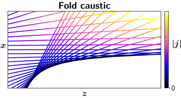
Figure 1: Ray trajectories for the fold caustic obtained via Eq. (25) with $\lambda=2\pi$, $\ell=\sqrt[3]{3}$, and $a_{1}=0$. The color shows the magnitude of the Jacobian $j({\boldsymbol{\rm\tau}})$ defined by Eq. (12). The caustic occurs where $j=0$ (black curve).

The simplest caustic of the cuspoid family is the $A_{2}$ fold caustic. The field near a fold caustic is given by Eq. (22), and the underlying ray trajectories are given by Eqs. (19) and (21); namely,

$$x(z,x_{0})=x_{0}+\frac{\lambda z}{2\pi\ell}\left(\frac{3x_{0}^{2}}{\ell^{2}}+a_{1}\right).$$ (25)

The fold caustic occurs where Eq. (15b) is satisfied, or equivalently, where $\partial_{x_{0}}x(z,x_{0})=0$. This ultimately yields the caustic curve

$$x_{c}(z)=a_{1}\frac{\lambda z}{2\pi\ell}-\frac{\pi\ell^{3}}{6\lambda z}.$$ (26)

The ray pattern (25) is shown in Fig. 1, in which the caustic curve (26) is clearly visible.

Let us next consider the $A_{3}$ cusp caustic. The field near a cusp caustic is given by Eq. (23) with $m=2$, and the underlying ray trajectories are given as

$$x(z,x_{0})=x_{0}+\frac{\lambda z}{2\pi\ell}\left(\frac{4x_{0}^{3}}{\ell^{3}}+a_{1}+a_{2}\frac{2x_{0}}{\ell}\right).$$ (27)

The cusp caustic can be shown to occur along the curve

$$x_{c}(z)=a_{1}\frac{\lambda z}{2\pi\ell}\pm\frac{\sqrt{-6\lambda z(\pi\ell^{2}+a_{2}\lambda z)^{3}}}{9\pi\ell\lambda z}.$$ (28)

The ray pattern (27) is shown in Fig. 2, in which the caustic curve (28) is clearly visible.

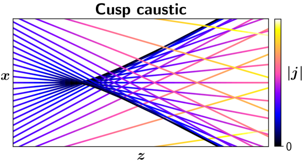
Figure 2: Same as Fig. 1 but for the cusp caustic (27) with $\lambda=2\pi$, $\ell=\sqrt{2}$, $a_{1}=0$, and $a_{2}=-2$.

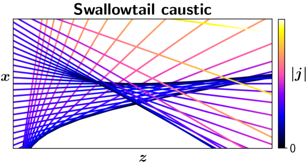
Figure 3: Same as Fig. 1 but for the swallowtail caustic (29) with $\lambda=2\pi$, $\ell=\sqrt[5]{5}$, $a_{1}=0$, $a_{2}=-1$, and $a_{3}=-1$.

Let us next consider the final stable cuspoid in $3$-D, the $A_{4}$ swallowtail caustic. Here, we shall choose to generate the swallowtail via the mathematically simpler approach of having the a high-order $1$-D aberration, rather than with a low-order $2$-D aberration as would more commonly occur in practice. Correspondingly, the field near a swallowtail caustic is given by Eq. (23) with $m=3$, and the underlying ray trajectories are given as

$$x(z,x_{0})=x_{0}+\frac{\lambda z}{2\pi\ell}\left(\frac{5x_{0}^{4}}{\ell^{4}}+a_{1}+a_{2}\frac{2x_{0}}{\ell}+a_{3}\frac{3x_{0}^{2}}{\ell^{2}}\right).$$ (29)

The cusp caustic can be shown to occur along the parametric curve

$$x_{c}(\zeta) =\frac{a_{1}\lambda z_{c}(\zeta)}{2\pi\ell}-\frac{3\lambda z_{c}(\zeta)}{2\pi\ell}(a_{3}+5\zeta^{2})\zeta^{2},$$ (30a)

$$z_{c}(\zeta) =-\frac{\pi\ell^{2}}{\lambda\left[a_{2}+\zeta(3a_{3}+10\zeta^{2})\right]},$$ (30b)

where $\zeta\in(-\infty,\infty)$ is a $1$-D parameterization of the caustic curve in the ($x$,$z$) plane. The ray pattern (29) is shown in Fig. 3 for parameters specifically chosen to have the eponymous swallowtail section of the caustic curve (30) appear in the longitudinal plane.

II.2.2 Umbilic caustics

Consider now $N=2$ (so the total number of spatial dimensions is three). In addition to the cuspoids, a new class of caustics, the umbilics, are now possible. A wavefield containing any caustic from the $D_{m+1}^{\pm}$ umbilic series can be generated by choosing

$$\psi({\boldsymbol{\rm x}},0)=\exp\left(i\frac{y^{m}}{\ell^{m}}\pm i\frac{x^{2}y}{\ell^{3}}+ia_{1}\frac{x}{\ell}+ia_{2}\frac{y}{\ell}+ia_{3}\frac{x^{2}}{\ell^{2}}+i\sum_{j=4}^{m}a_{j}\frac{y^{j-2}}{\ell^{j-2}}\right).$$ (31)

The corresponding solution (17b) for $m\geq 4$ is

$$\psi({\boldsymbol{\rm x}},z)=\frac{\ell^{2}}{i\lambda z}\exp\left(i\frac{\pi{\boldsymbol{\rm x}}^{\intercal}{\boldsymbol{\rm x}}}{\lambda z}\right)D_{m+1}^{\pm}\left(a_{1}-\frac{2\pi\ell x}{\lambda z},a_{2}-\frac{2\pi\ell y}{\lambda z},a_{3}+\frac{\pi\ell^{2}}{\lambda z},a_{4}+\frac{\pi\ell^{2}}{\lambda z},a_{5},\ldots,a_{m}\right),$$ (32)

while for $m=3$ is given as

$$\psi({\boldsymbol{\rm x}},z)=\frac{\ell^{2}}{i\lambda z}\exp\left(i\frac{\pi{\boldsymbol{\rm x}}^{\intercal}{\boldsymbol{\rm x}}}{\lambda z}-ia_{2}\frac{\pi\ell^{2}}{3\lambda z}+i\frac{2\pi^{2}\ell^{3}}{3\lambda^{2}z^{2}}y+i\frac{2\pi^{3}\ell^{6}}{27\lambda^{3}z^{3}}\right)D_{4}^{\pm}\left(a_{1}-\frac{2\pi\ell x}{\lambda z},a_{2}-\frac{2\pi\ell y}{\lambda z}-\frac{\pi^{2}\ell^{4}}{3\lambda^{2}z^{2}},a_{3}+\frac{3\mp 1}{3\lambda z}\pi\ell^{2}\right),$$ (33)

where the $D_{m+1}^{\pm}$ catastrophe integral is defined as

$$D_{m+1}^{\pm}\left(a_{1},\ldots,a_{m}\right)\doteq\int\mathrm{d}U\,\mathrm{d}V\exp\left[iV^{m}\pm iU^{2}V+ia_{1}U+ia_{2}V+ia_{3}U^{2}+i\sum_{j=4}^{m}a_{j}V^{j-2}\right].$$ (34)

Note that the initial condition (31) generates rays having

$$k_{x,0}({\boldsymbol{\rm x}}_{0})=\pm 2\frac{x_{0}y_{0}}{\ell^{3}}+\frac{a_{1}}{\ell}+2a_{3}\frac{x_{0}}{\ell^{2}},\quad k_{y,0}({\boldsymbol{\rm x}}_{0})=m\frac{y_{0}^{m-1}}{\ell^{m}}\pm\frac{x_{0}^{2}}{\ell^{3}}+\frac{a_{2}}{\ell}+\sum_{j=4}^{m}(j-2)a_{j}\frac{y_{0}^{j-3}}{\ell^{j-2}}.$$ (35)

The only umbilics that occur stably in $3$-D are the $D_{4}^{+}$ hyperbolic and the $D_{4}^{-}$ elliptic umbilic caustics. The field near these caustics are given by Eq. (33). The underlying ray trajectories for the hyperbolic umbilic are given as

$$x(z;{\boldsymbol{\rm x}}_{0}) =x_{0}+\frac{\lambda z}{2\pi\ell}\left(a_{1}+2a_{3}\frac{x_{0}}{\ell}+2\frac{x_{0}y_{0}}{\ell^{2}}\right),$$ (36a)

$$y(z;{\boldsymbol{\rm x}}_{0}) =y_{0}+\frac{\lambda z}{2\pi\ell}\left(a_{2}+\frac{3y_{0}^{2}+x_{0}^{2}}{\ell^{2}}\right),$$ (36b)

and the caustic in the $(x,y)$ transverse plane at fixed propagation distance $z$ is given by the parametric curve

$$x_{c}(\zeta) =a_{1}\frac{\lambda z}{2\pi\ell}-\frac{\sqrt{3}\lambda z}{4\pi\ell}\left(a_{3}+\frac{2\pi\ell^{2}}{3\lambda z}\right)^{2}$$

$$\hskip 82.51299pt\times\sinh(\zeta)\left[\cosh(\zeta)\pm 1\right],$$ (37a)

$$y_{c}(\zeta) =a_{2}\frac{\lambda z}{2\pi\ell}-\frac{\pi\ell^{3}}{6\lambda z}+\frac{3\lambda z}{4\pi\ell}\left(a_{3}+\frac{2\pi\ell^{2}}{3\lambda z}\right)^{2}$$

$$\hskip 82.51299pt\times\cosh(\zeta)\left[\cosh(\zeta)\mp 1\right].$$ (37b)

Figure 4: Intersection plot of the ray trajectories for the hyperbolic umbilic caustic obtained via Eq. (36) with $\lambda=4\pi$, $\ell=1$, $a_{1}=0$, $a_{2}=-1.3$, and $a_{3}=-1$ through the plane $z=1$.

Note that the hyperbolic umbilic actually contains two separate caustic curves (indicated by the $\pm$ terms above): a fold curve (top sign) and a cusp curve (bottom sign). These two curves lie in a squid-like orientation with the cusp residing within the bow of the fold. This is readily observed in Fig. 4, which presents an intersection plot for the rays (36) with respect to the plane $z=1$. As each dot represents a single traversing ray, the $D_{4}^{+}$ caustic (37) manifests as a visible increase in the ray density.

Similarly, the ray trajectories for the elliptic umbilic are given as

$$x(z;{\boldsymbol{\rm x}}_{0}) =x_{0}+\frac{\lambda z}{2\pi\ell}\left(a_{1}+2a_{3}\frac{x_{0}}{\ell}-2\frac{x_{0}y_{0}}{\ell^{2}}\right),$$ (38a)

$$y(z;{\boldsymbol{\rm x}}_{0}) =y_{0}+\frac{\lambda z}{2\pi\ell}\left(a_{2}+\frac{3y_{0}^{2}-x_{0}^{2}}{\ell^{2}}\right),$$ (38b)

with the caustic at a fixed distance $z$ given by the parametric curve

$$x_{c}(\zeta) =a_{1}\frac{\lambda z}{2\pi\ell}+\frac{\sqrt{3}\lambda z}{2\pi\ell}\left(a_{3}+\frac{4\pi\ell^{2}}{3\lambda z}\right)^{2}$$

$$\hskip 102.42992pt\times\sin^{2}\left(\frac{\zeta}{2}\right)\sin(\zeta),$$ (39a)

$$y_{c}(\zeta) =a_{2}\frac{\lambda z}{2\pi\ell}-\frac{\pi\ell^{3}}{6\lambda z}+\frac{3\lambda z}{2\pi\ell}\left(a_{3}+\frac{4\pi\ell^{2}}{3\lambda z}\right)^{2}$$

$$\hskip 102.42992pt\times\cos^{2}\left(\frac{\zeta}{2}\right)\cos(\zeta).$$ (39b)

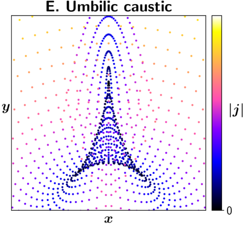
Figure 5: Same as Fig. 4 but for the elliptic umbilic caustic (38) with $\lambda=4\pi$, $\ell=1$, $a_{1}=0$, $a_{2}=-0.7$, and $a_{3}=-2.1$.

Figure 5 presents an intersection plot of the ray trajectories (38) that generate the $D_{4}^{-}$ caustic with respect to the plane $z=1$. The characteristic tricorn shape of the caustic curve (39) is readily observed by the visible increase in the ray density.

As mentioned, these five caustics constitute the complete set of caustics that can occur in $3$-D systems. Hence, a popular means of modeling caustics along rays is the method of ‘uniform approximation’ Berry and Upstill (1980); Kravtsov and Orlov (1993); Olver et al. (2010), which consists of fitting a given wavefield to one of these normal forms. Although this method has been used effectively by previous authors, notably by Ref. Colaitis et al., 2019 for modeling laser-plasma interactions near caustics, it suffers from the obvious disadvantage that the caustic type must be known beforehand or somehow guessed reliably. In the following section, we shall describe a different approach to dealing with caustics within ray optics. This alternate method is more general in that it does not assume any specific caustic type in advance, so it may be more convenient for practical calculations.

III Metaplectic geometrical optics: theory

III.1 Metaplectic operators to ‘rotate’ equations

By definition, Eq. (15b) is satisfied (and a caustic therefore occurs) where the ray manifold has a singular projection onto ${\boldsymbol{\rm x}}$-space. It stands to reason that removing caustics should be possible by continually rotating the ray manifold during the ray-tracing step (10) to maintain a good projection onto ${\boldsymbol{\rm x}}$-space at all points along a ray. This geometrical idea is the foundation for the MGO method of caustic-free ray tracing Lopez and Dodin (2020, 2021a).

To develop this mathematically, it is necessary to introduce some new machinery. Rather than describing waves as propagating in some configuration space with coordinates ${\boldsymbol{\rm x}}$ according to a pseudo-differential equation of the form (1), it is more natural to describe waves as state vectors $|\psi\rangle$ in a Hilbert space being acted upon by operators. Then, partial differential equations that govern wavefields can be understood as projections of the invariant wave equations

$$\smash{\hat{D}}(\smash{\hat{{\boldsymbol{\rm x}}}},\smash{\hat{{\boldsymbol{\rm k}}}})|\psi\rangle=|0\rangle$$ (40)

on a particular basis. In particular, Eq. (1) is the projection of Eq. (40) on the basis $\{|{\boldsymbol{\rm x}}({\boldsymbol{\rm y}})\rangle\}$ formed by the orthonormal eigenvectors of the coordinate operator $\smash{\hat{{\boldsymbol{\rm x}}}}$:

$$\smash{\hat{{\boldsymbol{\rm x}}}}|{\boldsymbol{\rm x}}({\boldsymbol{\rm y}})\rangle={\boldsymbol{\rm y}}|{\boldsymbol{\rm x}}({\boldsymbol{\rm y}})\rangle,\quad\langle{\boldsymbol{\rm x}}({\boldsymbol{\rm y}})|{\boldsymbol{\rm x}}({\boldsymbol{\rm y}}^{\prime})\rangle=\delta({\boldsymbol{\rm y}}-{\boldsymbol{\rm y}}^{\prime}),$$ (41)

and accordingly,

$$\psi({\boldsymbol{\rm y}})=\langle{\boldsymbol{\rm x}}({\boldsymbol{\rm y}})|\psi\rangle.$$ (42)

Likewise, the Fourier transform of Eq. (1) can be understood as the projection of Eq. (40) on the basis $\{|{\boldsymbol{\rm k}}({\boldsymbol{\rm\kappa}})\rangle\}$ formed by the orthonormal eigenvectors of the wavevector operator $\smash{\hat{{\boldsymbol{\rm k}}}}$:

$$\smash{\hat{{\boldsymbol{\rm k}}}}|{\boldsymbol{\rm k}}({\boldsymbol{\rm\kappa}})\rangle={\boldsymbol{\rm\kappa}}|{\boldsymbol{\rm k}}({\boldsymbol{\rm\kappa}})\rangle,\quad\langle{\boldsymbol{\rm k}}({\boldsymbol{\rm\kappa}})|{\boldsymbol{\rm k}}({\boldsymbol{\rm\kappa}}^{\prime})\rangle=\delta({\boldsymbol{\rm\kappa}}-{\boldsymbol{\rm\kappa}}^{\prime}).$$ (43)

As usual Shankar (1994),

$$\int\mathrm{d}{\boldsymbol{\rm y}}\,|{\boldsymbol{\rm x}}({\boldsymbol{\rm y}})\rangle\langle{\boldsymbol{\rm x}}({\boldsymbol{\rm y}})|=\int\mathrm{d}{\boldsymbol{\rm\kappa}}\,|{\boldsymbol{\rm k}}({\boldsymbol{\rm\kappa}})\rangle\langle{\boldsymbol{\rm k}}({\boldsymbol{\rm\kappa}})|=\smash{\hat{\mathds{1}}},$$ (44)

where $\smash{\hat{\mathds{1}}}$ is the identity operator, and also

$$\langle{\boldsymbol{\rm x}}({\boldsymbol{\rm y}})|\smash{\hat{{\boldsymbol{\rm x}}}}|{\boldsymbol{\rm x}}({\boldsymbol{\rm y}}^{\prime})\rangle ={\boldsymbol{\rm y}}\delta({\boldsymbol{\rm y}}-{\boldsymbol{\rm y}}^{\prime}),$$ (45a)

$$\langle{\boldsymbol{\rm x}}({\boldsymbol{\rm y}})|\smash{\hat{{\boldsymbol{\rm k}}}}|{\boldsymbol{\rm x}}({\boldsymbol{\rm y}}^{\prime})\rangle =-i\partial_{{\boldsymbol{\rm y}}}\delta({\boldsymbol{\rm y}}-{\boldsymbol{\rm y}}^{\prime}),$$ (45b)

$$\langle{\boldsymbol{\rm k}}({\boldsymbol{\rm\kappa}})|\smash{\hat{{\boldsymbol{\rm x}}}}|{\boldsymbol{\rm k}}({\boldsymbol{\rm\kappa}}^{\prime})\rangle =i\partial_{{\boldsymbol{\rm\kappa}}}\delta({\boldsymbol{\rm\kappa}}-{\boldsymbol{\rm\kappa}}^{\prime}),$$ (45c)

$$\langle{\boldsymbol{\rm k}}({\boldsymbol{\rm\kappa}})|\smash{\hat{{\boldsymbol{\rm k}}}}|{\boldsymbol{\rm k}}({\boldsymbol{\rm\kappa}}^{\prime})\rangle ={\boldsymbol{\rm\kappa}}\delta({\boldsymbol{\rm\kappa}}-{\boldsymbol{\rm\kappa}}^{\prime}).$$ (45d)

Equations (45) show that in the ${\boldsymbol{\rm x}}$ representation [i.e., projection on the $\{|{\boldsymbol{\rm x}}({\boldsymbol{\rm y}})\rangle\}$ basis], one has

$$\smash{\hat{{\boldsymbol{\rm x}}}}\mapsto{\boldsymbol{\rm x}},\quad\smash{\hat{{\boldsymbol{\rm k}}}}\mapsto-i\partial_{{\boldsymbol{\rm x}}},$$ (46)

while in the ${\boldsymbol{\rm k}}$ representation [i.e., projection on the $\{|{\boldsymbol{\rm k}}({\boldsymbol{\rm\kappa}})\rangle\}$ basis], one has

$$\smash{\hat{{\boldsymbol{\rm x}}}}\mapsto i\partial_{{\boldsymbol{\rm k}}},\quad\smash{\hat{{\boldsymbol{\rm k}}}}\mapsto{\boldsymbol{\rm k}}.$$ (47)

However, the ${\boldsymbol{\rm x}}$ representation and the ${\boldsymbol{\rm k}}$ representation are not the only ones possible. Instead, one can consider a different ${\boldsymbol{\rm X}}$ representation in which caustics of the wavefield vanish, at least locally. This is done as follows.

Suppose ${\boldsymbol{\rm X}}$ is related to the original representation ${\boldsymbol{\rm x}}$ by a linear canonical transformation of the form

$$\text{\ooalign{${\boldsymbol{\rm Z}}$\cr\raise 0.96877pt\hbox{$-\mkern 0.5mu$}\cr}}=\mathsf{S}{\boldsymbol{\rm z}},$$ (48)

where ${\boldsymbol{\rm Z}}$ $-\mkern 0.5mu$ and ${\boldsymbol{\rm z}}$ are transformed and original phase-space coordinates, respectively, i.e.,

$$\text{\ooalign{${\boldsymbol{\rm Z}}$\cr\raise 0.96877pt\hbox{$-\mkern 0.5mu$}\cr}}\doteq\begin{pmatrix}{\boldsymbol{\rm X}}\\ {\boldsymbol{\rm K}}\end{pmatrix},\quad{\boldsymbol{\rm z}}\doteq\begin{pmatrix}{\boldsymbol{\rm x}}\\ {\boldsymbol{\rm k}}\end{pmatrix}$$ (49)

(where ${\boldsymbol{\rm K}}$ is the phase-space dual coordinate to ${\boldsymbol{\rm X}}$), and the $2N\times 2N$ transformation matrix $\mathsf{S}$ is symplectic, satisfying

$$\mathsf{S}^{\intercal}\mathsf{J}_{2N}\mathsf{S}=\mathsf{J}_{2N}.$$ (50)

As we shall show in Sec. IV.2, for MGO we can further impose that $\mathsf{S}$ be orthogonal in addition to being symplectic (orthosymplectic). This means that $\mathsf{S}$ also satisfies

$$\mathsf{S}^{\intercal}=\mathsf{S}^{-1}.$$ (51)

Together, Eqs. (50) and (51) imply that $\mathsf{S}$ can be represented by block decomposition Littlejohn (1986b)

$$\mathsf{S}=\begin{pmatrix}\mathsf{A}&\mathsf{B}\\ -\mathsf{B}&\mathsf{A}\end{pmatrix},$$ (52)

where the $N\times N$ submatrices $\mathsf{A}$ and $\mathsf{B}$ satisfy

$$\mathsf{A}\mathsf{A}^{\intercal}+\mathsf{B}\mathsf{B}^{\intercal} =\mathsf{I}_{N},$$ (53a)

$$\mathsf{A}^{\intercal}\mathsf{A}+\mathsf{B}^{\intercal}\mathsf{B} =\mathsf{I}_{N},$$ (53b)

$$\mathsf{A}\mathsf{B}^{\intercal}-\mathsf{B}\mathsf{A}^{\intercal} =\mathsf{0}_{N},$$ (53c)

$$\mathsf{B}^{\intercal}\mathsf{A}-\mathsf{A}^{\intercal}\mathsf{B} =\mathsf{0}_{N}.$$ (53d)

Linear symplectic phase-space transformations are special because they have an exact operator analogue in a Hilbert space; these are the unitary metaplectic operators Moshinsky and Quesne (1971); Littlejohn (1986b), denoted as $\smash{\hat{M}}(\mathsf{S})$. Specifically, the corresponding operators $\smash{\hat{{\boldsymbol{\rm z}}}}$ and $\smash{\hat{{\boldsymbol{\rm Z}}}}\doteq(\smash{\hat{{\boldsymbol{\rm X}}}},\smash{\hat{{\boldsymbol{\rm K}}}})^{\intercal}$ are related as

$$\text{\ooalign{$\smash{\hat{{\boldsymbol{\rm Z}}}}$\cr\raise 0.96877pt\hbox{$-\mkern 0.5mu$}\cr}}=\smash{\hat{M}}^{\dagger}(\mathsf{S})\smash{\hat{{\boldsymbol{\rm z}}}}\smash{\hat{M}}(\mathsf{S})\equiv\mathsf{S}\smash{\hat{{\boldsymbol{\rm z}}}},$$ (54)

or equivalently in terms of the constituent operators ,

$$\smash{\hat{{\boldsymbol{\rm X}}}} =\smash{\hat{M}}^{\dagger}(\mathsf{S})\smash{\hat{{\boldsymbol{\rm x}}}}\smash{\hat{M}}(\mathsf{S})\equiv\mathsf{A}\smash{\hat{{\boldsymbol{\rm x}}}}+\mathsf{B}\smash{\hat{{\boldsymbol{\rm k}}}},$$ (55a)

$$\smash{\hat{{\boldsymbol{\rm K}}}} =\smash{\hat{M}}^{\dagger}(\mathsf{S})\smash{\hat{{\boldsymbol{\rm k}}}}\smash{\hat{M}}(\mathsf{S})\equiv-\mathsf{B}\smash{\hat{{\boldsymbol{\rm x}}}}+\mathsf{A}\smash{\hat{{\boldsymbol{\rm k}}}},$$ (55b)

Also, $\smash{\hat{M}}$ directly generates the basis transformation as

$$|{\boldsymbol{\rm X}}({\boldsymbol{\rm y}})\rangle=\smash{\hat{M}}^{\dagger}(\mathsf{S})|{\boldsymbol{\rm x}}({\boldsymbol{\rm y}})\rangle.$$ (56)

The matrix elements of $\smash{\hat{M}}$ in the ${\boldsymbol{\rm x}}$ representation, which govern the overlap between the ${\boldsymbol{\rm x}}$ and ${\boldsymbol{\rm X}}$ representations, are given for invertible $\mathsf{B}$ as Moshinsky and Quesne (1971); Littlejohn (1986b)

$$\langle{\boldsymbol{\rm X}}({\boldsymbol{\rm Y}})|{\boldsymbol{\rm x}}({\boldsymbol{\rm y}})\rangle =\langle{\boldsymbol{\rm x}}({\boldsymbol{\rm Y}})|\smash{\hat{M}}(\mathsf{S})|{\boldsymbol{\rm x}}({\boldsymbol{\rm y}})\rangle$$

$$=\frac{\sigma\exp[iG({\boldsymbol{\rm y}},{\boldsymbol{\rm Y}})]}{(2\pi i)^{N/2}\sqrt{\det\mathsf{B}}},$$ (57)

where $G({\boldsymbol{\rm y}},{\boldsymbol{\rm Y}})$ is the quadratic generator function

$$G({\boldsymbol{\rm y}},{\boldsymbol{\rm Y}}) =\frac{1}{2}{\boldsymbol{\rm y}}^{\intercal}\mathsf{B}^{-1}\mathsf{A}{\boldsymbol{\rm y}}-{\boldsymbol{\rm y}}^{\intercal}\mathsf{B}^{-1}{\boldsymbol{\rm Y}}+\frac{1}{2}{\boldsymbol{\rm Y}}^{\intercal}\mathsf{A}\mathsf{B}^{-1}{\boldsymbol{\rm Y}},$$ (58)

and $\sigma\doteq\pm 1$. The sign ambiguity in $\sigma$ is of fundamental importance, as it contributes to the well-known phase shifts that a wavefield acquires upon touching a caustic Littlejohn (1986b); Lopez and Dodin (2019); Berry and Mount (1972); Littlejohn and Robbins (1987); Ciobanu et al. (2021), the $\pi/2$ phase shift following reflection being a famous example. Note that when $\det{\mathsf{B}}=0$, the right-hand side of Eq. (57) becomes a delta function over the singular subspace of $\mathsf{B}$ Moshinsky and Quesne (1971); Littlejohn (1986b).

Accordingly, wavefunctions (i.e., projections of state vectors $|\psi\rangle$, not the invariant state vectors themselves) are transformed via Eq. (44) as

$$\smash{\widetilde{\psi}}({\boldsymbol{\rm Y}})\doteq\langle{\boldsymbol{\rm X}}({\boldsymbol{\rm Y}})|\psi\rangle =\int\mathrm{d}{\boldsymbol{\rm y}}\langle{\boldsymbol{\rm X}}({\boldsymbol{\rm Y}})|{\boldsymbol{\rm x}}({\boldsymbol{\rm y}})\rangle\langle{\boldsymbol{\rm x}}({\boldsymbol{\rm y}})|\psi\rangle$$

$$=\int\mathrm{d}{\boldsymbol{\rm y}}\,\frac{\sigma\exp[iG({\boldsymbol{\rm y}},{\boldsymbol{\rm Y}})]}{(2\pi i)^{N/2}\sqrt{\det\mathsf{B}}}\,\psi({\boldsymbol{\rm y}}).$$ (59)

Equation (59) is called the metaplectic transform (MT). Special cases include the $N$-D Fourier transform ($\mathsf{A}=\mathsf{0}_{N}$, $\mathsf{B}=\mathsf{I}_{N}$) and the Fresnel transform (17b) (for which $\mathsf{S}$ is not orthogonal, but is instead given by the ray transfer matrix for propagation in uniform media Kogelnik and Li (1966)). The inverse MT is given similarly as

$$\psi({\boldsymbol{\rm y}})=\int\mathrm{d}{\boldsymbol{\rm Y}}\,\frac{\sigma\exp[-iG({\boldsymbol{\rm y}},{\boldsymbol{\rm Y}})]}{(-2\pi i)^{N/2}\sqrt{\det\mathsf{B}}}\,\smash{\widetilde{\psi}}({\boldsymbol{\rm Y}}).$$ (60)

Let us now discuss how these tools enable the development of a caustic-free GO formalism called metaplectic geometrical optics.

III.2 MGO formulas for scalar wavefields

Suppose that $|\psi\rangle$ exhibits a caustic in the ${\boldsymbol{\rm x}}$ representation but has an eikonal form in the ${\boldsymbol{\rm X}}$ representation:

$$\smash{\widetilde{\psi}}({\boldsymbol{\rm Y}})=\smash{\widetilde{\phi}}({\boldsymbol{\rm Y}})\exp[i\Theta({\boldsymbol{\rm Y}})],$$ (61)

where $\Theta$ is a rapidly varying and $\smash{\widetilde{\phi}}$ is a slowly varying function of ${\boldsymbol{\rm Y}}$, analogous to Eq. (2). In the invariant form, Eq. (61) can be written as

$$|\psi\rangle=\smash{\hat{U}}(\smash{\hat{{\boldsymbol{\rm X}}}})|\phi\rangle,\quad\smash{\hat{U}}(\smash{\hat{{\boldsymbol{\rm X}}}})\doteq\exp[i\Theta(\smash{\hat{{\boldsymbol{\rm X}}}})].$$ (62)

The unitary operator $\smash{\hat{U}}$ can be considered as a transformation connecting the complete wavefield $\smash{\widetilde{\psi}}$ with its envelope $\smash{\widetilde{\phi}}$, since

$$\langle{\boldsymbol{\rm X}}({\boldsymbol{\rm Y}})|\smash{\hat{U}}^{\dagger}(\smash{\hat{{\boldsymbol{\rm X}}}})|\psi\rangle =\exp[-i\Theta({\boldsymbol{\rm Y}})]\smash{\widetilde{\phi}}({\boldsymbol{\rm Y}})\exp[i\Theta({\boldsymbol{\rm Y}})]$$

$$\equiv\smash{\widetilde{\phi}}({\boldsymbol{\rm Y}}).$$ (63)

Then, the wave equation (1) can be written as an envelope equation

$$\smash{\hat{U}}^{\dagger}(\smash{\hat{{\boldsymbol{\rm X}}}})\smash{\hat{D}}(\mathsf{S}^{-1}\text{\ooalign{$\smash{\hat{{\boldsymbol{\rm Z}}}}$\cr\raise 0.96877pt\hbox{$-\mkern 0.5mu$}\cr}})\smash{\hat{U}}(\smash{\hat{{\boldsymbol{\rm X}}}})|\phi\rangle=|0\rangle,$$ (64)

where we used Eq. (54) for $\smash{\hat{{\boldsymbol{\rm z}}}}$.

Following Refs. Dodin et al., 2019; Lopez and Dodin, 2020, Eq. (64) can be approximated in the GO limit by use of the Wigner–Weyl transform and the Moyal product (Appendix A), much like they are used for deriving traditional GO. Indeed, the GO-approximated envelope operator is obtained by first calculating the appropriate symbol, then approximating the symbol in the GO limit using familiar Taylor expansions, and finally mapping the symbol back to obtain the correspondingly approximated operator. Mathematically, this reads

$$\smash{\hat{U}}^{\dagger}(\smash{\hat{{\boldsymbol{\rm X}}}})\smash{\hat{D}}(\mathsf{S}^{-1}\text{\ooalign{$\smash{\hat{{\boldsymbol{\rm Z}}}}$\cr\raise 0.96877pt\hbox{$-\mkern 0.5mu$}\cr}})\smash{\hat{U}}(\smash{\hat{{\boldsymbol{\rm X}}}})$$ (67)

$$=\mathbb{W}^{-1}\left\{\mathbb{W}\left[\smash{\hat{U}}^{\dagger}(\smash{\hat{{\boldsymbol{\rm X}}}})\smash{\hat{D}}(\mathsf{S}^{-1}\text{\ooalign{$\smash{\hat{{\boldsymbol{\rm Z}}}}$\cr\raise 0.96877pt\hbox{$-\mkern 0.5mu$}\cr}})\smash{\hat{U}}(\smash{\hat{{\boldsymbol{\rm X}}}})\right]\right\}$$ (70)

$$=\mathbb{W}^{-1}\left[\mathcal{U}^{*}({\boldsymbol{\rm X}})\star\mathcal{D}(\mathsf{S}^{-1}\text{\ooalign{${\boldsymbol{\rm Z}}$\cr\raise 0.96877pt\hbox{$-\mkern 0.5mu$}\cr}})\star\mathcal{U}({\boldsymbol{\rm X}})\right]$$ (73)

$$\approx\mathbb{W}^{-1}\left\{\mathcal{D}[\mathsf{S}^{-1}\text{\ooalign{${\boldsymbol{\rm Z}}$\cr\raise 0.96877pt\hbox{$-\mkern 0.5mu$}\cr}}({\boldsymbol{\rm X}})]+{\boldsymbol{\rm K}}^{\intercal}{\boldsymbol{\rm V}}({\boldsymbol{\rm X}})+\ldots\right\}$$ (76)

$$=\mathcal{D}[\mathsf{S}^{-1}\text{\ooalign{${\boldsymbol{\rm Z}}$\cr\raise 0.96877pt\hbox{$-\mkern 0.5mu$}\cr}}(\smash{\hat{{\boldsymbol{\rm X}}}})]+{\boldsymbol{\rm V}}(\smash{\hat{{\boldsymbol{\rm X}}}})^{\intercal}\smash{\hat{{\boldsymbol{\rm K}}}}-\frac{i}{2}\nabla\cdot{\boldsymbol{\rm V}}(\smash{\hat{{\boldsymbol{\rm X}}}})+\ldots,$$ (79)

where we have introduced

$$\text{\ooalign{${\boldsymbol{\rm Z}}$\cr\raise 0.96877pt\hbox{$-\mkern 0.5mu$}\cr}}({\boldsymbol{\rm X}}) \doteq\begin{pmatrix}{\boldsymbol{\rm X}}&\partial_{{\boldsymbol{\rm X}}}\Theta({\boldsymbol{\rm X}})\end{pmatrix}^{\intercal},$$ (80c)

$${\boldsymbol{\rm V}}({\boldsymbol{\rm X}}) \doteq\partial_{{\boldsymbol{\rm K}}}\mathcal{D}\left[\mathsf{S}^{-1}\text{\ooalign{${\boldsymbol{\rm Z}}$\cr\raise 0.96877pt\hbox{$-\mkern 0.5mu$}\cr}}({\boldsymbol{\rm X}})\right].$$ (80f)

(Only first-order terms are included in the expansion (79) for simplicity; higher-order terms to enable beam-tracing of arbitrarily structured light Yanagihara et al. (2019a, b, 2021a, 2021b) can be readily included within this framework Lopez and Dodin (2020).) Hence, the GO-approximated equation that governs $\smash{\widetilde{\phi}}$ is obtained by projecting Eq. (79) onto the $|{\boldsymbol{\rm X}}({\boldsymbol{\rm Y}})\rangle$ basis:

$$\left\{\mathcal{D}[\mathsf{S}^{-1}\text{\ooalign{${\boldsymbol{\rm Z}}$\cr\raise 0.96877pt\hbox{$-\mkern 0.5mu$}\cr}}({\boldsymbol{\rm Y}})]-i{\boldsymbol{\rm V}}({\boldsymbol{\rm Y}})^{\intercal}\partial_{{\boldsymbol{\rm Y}}}-\frac{i}{2}\left[\nabla\cdot{\boldsymbol{\rm V}}({\boldsymbol{\rm Y}})\right]\right\}\smash{\widetilde{\phi}}({\boldsymbol{\rm Y}})=0.$$ (83)

Analogous to Eqs. (3) and (4), Eq. (83) is solved in two parts. First, the rotated dispersion relation,

$$\mathcal{D}[\mathsf{S}^{-1}\text{\ooalign{${\boldsymbol{\rm Z}}$\cr\raise 0.96877pt\hbox{$-\mkern 0.5mu$}\cr}}({\boldsymbol{\rm X}})]=0,$$ (84)

is solved (via ray-tracing) to obtain $\Theta$. Then, the rotated envelope equation,

$$2{\boldsymbol{\rm V}}({\boldsymbol{\rm X}})^{\intercal}\partial_{{\boldsymbol{\rm X}}}\smash{\widetilde{\phi}}({\boldsymbol{\rm X}})+\left[\nabla\cdot{\boldsymbol{\rm V}}({\boldsymbol{\rm X}})\right]\smash{\widetilde{\phi}}({\boldsymbol{\rm X}})=0,$$ (85)

is solved to obtain $\smash{\widetilde{\phi}}$. Having the same formal structure as Eqs. (3) and (4), the solutions to Eqs. (84) and (85) can be inferred from the known solutions ${\boldsymbol{\rm z}}({\boldsymbol{\rm\tau}})$ and $\phi({\boldsymbol{\rm\tau}})$ for the unrotated equations: Eq. (84) is solved by the rotated rays (equivalently, by the rotated ray manifold)

$$\text{\ooalign{${\boldsymbol{\rm Z}}$\cr\raise 0.96877pt\hbox{$-\mkern 0.5mu$}\cr}}({\boldsymbol{\rm\tau}})=\mathsf{S}{\boldsymbol{\rm z}}({\boldsymbol{\rm\tau}}),$$ (86)

and Eq. (85) is solved along the rotated rays as

$$\smash{\widetilde{\phi}}({\boldsymbol{\rm\tau}})=\smash{\widetilde{\phi}}_{0}({\boldsymbol{\rm\tau}}_{\perp})\sqrt{\frac{J_{0}({\boldsymbol{\rm\tau}}_{\perp})}{J({\boldsymbol{\rm\tau}})}},$$ (87)

where the Jacobian

$$J({\boldsymbol{\rm\tau}})\doteq\det\partial_{{\boldsymbol{\rm\tau}}}{\boldsymbol{\rm X}}({\boldsymbol{\rm\tau}})$$ (88)

governs the projection properties of the ray manifold onto the rotated ${\boldsymbol{\rm X}}$-space rather than ${\boldsymbol{\rm x}}$-space.

Equation (87) implies that a caustic at some position ${\boldsymbol{\rm\tau}}={\boldsymbol{\rm t}}$ on the ray manifold can be avoided by choosing ${\boldsymbol{\rm X}}$ to be the tangent plane at ${\boldsymbol{\rm t}}$, since $J({\boldsymbol{\rm t}})\neq 0$ is then guaranteed by definition. This is the logic of the MGO framework, which is summarized in three steps. First, the rotated GO equations (84) and (85) are solved in the tangent plane at a given ray position ${\boldsymbol{\rm t}}$. Next, the obtained solution $\smash{\widetilde{\psi}}({\boldsymbol{\rm X}})$ is rotated into the following tangent plane at ${\boldsymbol{\rm t}}+\delta{\boldsymbol{\rm t}}$ using an infinitesimal near-identity MT (NIMT) to provide initial conditions for the corresponding next set of rotated GO equations to be solved. This step improves the continuity of the global solution. In parallel, $\smash{\widetilde{\psi}}({\boldsymbol{\rm X}})$ is mapped back to the original ${\boldsymbol{\rm x}}$ coordinates using an inverse MT. This is repeated for all points on the ray manifold, resulting in an approximate solution of the form

$$\psi({\boldsymbol{\rm x}})=\sum_{{\boldsymbol{\rm t}}\in{\boldsymbol{\rm\tau}}({\boldsymbol{\rm x}})}\mathcal{N}_{\boldsymbol{\rm t}}({\boldsymbol{\rm x}})\,\Upsilon_{\boldsymbol{\rm t}}({\boldsymbol{\rm x}}),$$ (89)

where the sum is taken over all ray contributions that arrive at a given point ${\boldsymbol{\rm x}}$, similar to Eq. (14).

The analysis to obtain specific expressions for $\mathcal{N}_{\boldsymbol{\rm t}}({\boldsymbol{\rm x}})$ and $\Upsilon_{\boldsymbol{\rm t}}({\boldsymbol{\rm x}})$ is quite involved; let us therefore simply quote the final results when $\det\mathsf{B}\neq 0$ Lopez and Dodin (2020):

$$\mathcal{N}_{\boldsymbol{\rm t}}({\boldsymbol{\rm x}}) =\frac{\sigma_{\boldsymbol{\rm t}}\,\alpha_{\boldsymbol{\rm t}}\exp\left\{-iG_{\boldsymbol{\rm t}}[{\boldsymbol{\rm x}},{\boldsymbol{\rm X}}_{\boldsymbol{\rm t}}({\boldsymbol{\rm t}})]\vphantom{\frac{}{}}\right\}}{(-2\pi i)^{N/2}\sqrt{\det{\mathsf{B}_{\boldsymbol{\rm t}}}}},$$ (90)

$$\Upsilon_{\boldsymbol{\rm t}}({\boldsymbol{\rm x}}) =\int_{\mathcal{C}_{0}}\mathrm{d}{\boldsymbol{\rm\epsilon}}\,\smash{\widetilde{\psi}}\left[{\boldsymbol{\rm\epsilon}}+{\boldsymbol{\rm X}}_{\boldsymbol{\rm t}}({\boldsymbol{\rm t}})\right]\exp\left[-i\gamma_{\boldsymbol{\rm t}}({\boldsymbol{\rm\epsilon}},{\boldsymbol{\rm x}})\right],$$ (91)

where we have introduced $\mathsf{S}_{\boldsymbol{\rm t}}$ as the matrix that rotates ${\boldsymbol{\rm x}}$ to the tangent plane at ${\boldsymbol{\rm t}}$, $\sigma_{\boldsymbol{\rm t}}$ as an overall sign such that $\sigma_{\boldsymbol{\rm t}}/\sqrt{\det\mathsf{B}_{\boldsymbol{\rm t}}}$ is continuous across any branch cuts, and $\mathcal{C}_{0}$ as the steepest-descent contour that passes through the origin ${\boldsymbol{\rm\epsilon}}={\boldsymbol{\rm 0}}$. The functions $G_{\boldsymbol{\rm t}}$ and ${\boldsymbol{\rm X}}_{\boldsymbol{\rm t}}$ are determined by Eqs. (58) and (86) for $\mathsf{S}_{\boldsymbol{\rm t}}$, respectively. We have also defined

$$\gamma_{\boldsymbol{\rm t}}({\boldsymbol{\rm\epsilon}},{\boldsymbol{\rm x}}) \doteq\frac{1}{2}{\boldsymbol{\rm\epsilon}}^{\intercal}\mathsf{A}_{\boldsymbol{\rm t}}\mathsf{B}_{\boldsymbol{\rm t}}^{-1}{\boldsymbol{\rm\epsilon}}+{\boldsymbol{\rm\epsilon}}^{\intercal}\mathsf{B}_{\boldsymbol{\rm t}}^{-\intercal}\left[\mathsf{A}_{\boldsymbol{\rm t}}^{\intercal}{\boldsymbol{\rm X}}_{\boldsymbol{\rm t}}({\boldsymbol{\rm t}})-{\boldsymbol{\rm x}}\right],$$ (92)

along with the continuity factor $\alpha_{\boldsymbol{\rm t}}$ that can be evolved along a ray via the NIMT as

$$\alpha_{{\boldsymbol{\rm t}}+{\boldsymbol{\rm h}}}=\alpha_{\boldsymbol{\rm t}}\left.\mathbb{N}_{\mathsf{S}_{{\boldsymbol{\rm t}}+{\boldsymbol{\rm h}}}\mathsf{S}^{-1}_{\boldsymbol{\rm t}}}\left[\smash{\widetilde{\psi}}({\boldsymbol{\rm X}})\right]\right|_{{\boldsymbol{\rm X}}={\boldsymbol{\rm X}}_{{\boldsymbol{\rm t}}+{\boldsymbol{\rm h}}}({\boldsymbol{\rm t}}+{\boldsymbol{\rm h}})},$$ (93)

where $\mathbb{N}_{\mathsf{S}}$ denotes the NIMT corresponding to a given near-identity symplectic transformation $\mathsf{S}$. Equivalently, as shown in Appendix D, $\alpha_{\boldsymbol{\rm t}}$ can be computed as

$$\alpha_{\boldsymbol{\rm t}} =f({\boldsymbol{\rm t}}_{\perp})\exp\left[\frac{i}{2}{\boldsymbol{\rm K}}^{\intercal}_{\boldsymbol{\rm t}}({\boldsymbol{\rm t}}){\boldsymbol{\rm X}}_{\boldsymbol{\rm t}}({\boldsymbol{\rm t}})+\int_{0}^{t_{1}}\mathrm{d}\xi\,\eta_{(\xi,{\boldsymbol{\rm t}}_{\perp})}\right],$$ (94)

$$\eta_{\boldsymbol{\rm t}} \doteq-\frac{i}{2}{\boldsymbol{\rm z}}^{\intercal}({\boldsymbol{\rm t}})\,\mathsf{J}_{2N}\,\dot{{\boldsymbol{\rm z}}}({\boldsymbol{\rm t}})$$

$$\hskip 11.38109pt+\left[\mathsf{A}_{\boldsymbol{\rm t}}\dot{{\boldsymbol{\rm x}}}({\boldsymbol{\rm t}})+\mathsf{B}_{\boldsymbol{\rm t}}\dot{{\boldsymbol{\rm k}}}({\boldsymbol{\rm t}})\right]^{\intercal}\partial_{{\boldsymbol{\rm X}}}\smash{\widetilde{\phi}}\left[{\boldsymbol{\rm X}}_{\boldsymbol{\rm t}}({\boldsymbol{\rm t}})\right],$$ (95)

where $f({\boldsymbol{\rm t}}_{\perp})$ is set by initial conditions and the dot $\cdot$ denotes $\partial_{t_{1}}$, i.e., the directional derivative along a ray. Accordingly, Eq. (90) can be shown to take the form

$$\mathcal{N}_{\boldsymbol{\rm t}}({\boldsymbol{\rm x}})=\frac{\sigma_{\boldsymbol{\rm t}}\,f({\boldsymbol{\rm t}}_{\perp})\exp\left[\frac{i}{2}{\boldsymbol{\rm x}}^{\intercal}{\boldsymbol{\rm k}}({\boldsymbol{\rm t}})+\int_{0}^{t_{1}}\mathrm{d}\xi\,\eta_{(\xi,{\boldsymbol{\rm t}}_{\perp})}\right]}{(-2\pi i)^{N/2}\sqrt{\det{\mathsf{B}_{\boldsymbol{\rm t}}}}}.$$ (96)

Equations (94)–(96) are considerably simpler than the expressions obtained previously in Refs. Lopez and Dodin, 2020, 2021a; this is largely because the orthosymplecticity of $\mathsf{S}$ implies that $\dot{\mathsf{S}}\mathsf{S}^{-1}$ is an antisymmetric Hamiltonian matrix, rather than simply a Hamiltonian matrix when $\mathsf{S}$ is merely symplectic.

Note that $\smash{\widetilde{\psi}}({\boldsymbol{\rm X}})$ should be normalized identically for all tangent planes, since any discrepancy in the normalization is already accounted for by $\alpha_{\boldsymbol{\rm t}}$ [specifically by the final term in Eq. (95)]. We also note that the final simplification (96) holds even when $\mathsf{B}$ is not invertible. For MGO formulas when $\det\mathsf{B}=0$ or an alternate MGO formulation that is insensitive to $\det\mathsf{B}$, see Appendix B and Appendix C, respectively.

The steepest-descent integration of Eq. (91) ensures that only points around ${\boldsymbol{\rm t}}$ on the ray manifold contribute to the MT integral, since only these ray contributions are guaranteed to be caustic-free by our construction. Such ‘saddlepoint filters’ tend to differ between otherwise similar phase-space rotation schemes; for example, Ref. Littlejohn, 1985 uses phase-space translation operators and a delta-shaped envelope model (Sec. III.4). Our formalism is flexible enough to allow modeling a variety of caustics in a variety of wave systems; to date, MGO has been used to model a caustic-free plane wave, an isolated fold caustic, a simple fold-caustic network, and an isolated cusp caustic in unidirectional, Helmholtz-like, and paraxial wave equations Lopez and Dodin (2020, 2021a); Donnelly et al. (2021). However, modeling the higher-order caustics discussed in Sec. II.2 requires a numerical implementation of MGO, which we shall discuss in Sec. IV.

III.3 Reducing MGO to standard GO away from caustics

In Refs. Lopez and Dodin, 2020, 2021a, it was shown numerically in a series of examples that the MGO formula (89) remains finite at caustics and agrees with the standard GO formula (14) away from caustics. The fact that (89) remains finite at caustics follows immediately from the observation that all terms in Eqs. (89)–(96) remain finite at caustics by construction; however, the fact that MGO reproduces GO away from caustics is less immediately obvious. In this section, we shall prove this property explicitly.

Let us assume that $\mathsf{B}_{\boldsymbol{\rm t}}$ is invertible for simplicity. Assuming that ${\boldsymbol{\rm x}}$ is located far from a caustic, $\Upsilon_{\boldsymbol{\rm t}}({\boldsymbol{\rm x}})$ can be evaluated by the standard (quadratic) saddlepoint method as follows:

$$\Upsilon_{\boldsymbol{\rm t}}({\boldsymbol{\rm x}}) \approx\int_{\mathcal{C}_{0}}\mathrm{d}{\boldsymbol{\rm\epsilon}}\,\exp\left\{i{\boldsymbol{\rm\epsilon}}^{\intercal}{\boldsymbol{\rm K}}_{\boldsymbol{\rm t}}({\boldsymbol{\rm t}})-i\gamma_{\boldsymbol{\rm t}}({\boldsymbol{\rm\epsilon}},{\boldsymbol{\rm x}})\right\}$$

$$=\int_{\mathcal{C}_{0}}\mathrm{d}{\boldsymbol{\rm\epsilon}}\,\exp\left\{-\frac{i}{2}{\boldsymbol{\rm\epsilon}}^{\intercal}\mathsf{A}_{\boldsymbol{\rm t}}\mathsf{B}_{\boldsymbol{\rm t}}^{-1}{\boldsymbol{\rm\epsilon}}\right\}$$

$$=\frac{(-2\pi i)^{N/2}\sqrt{\det\mathsf{B}_{\boldsymbol{\rm t}}}}{\sqrt{\det{\mathsf{A}_{\boldsymbol{\rm t}}}}},$$ (97)

where we have used the consistent normalization $\smash{\widetilde{\psi}}\left[{\boldsymbol{\rm X}}_{\boldsymbol{\rm t}}({\boldsymbol{\rm t}})\right]=1$ [see discussion following Eq. (96)], along with the fact that the second derivatives of the phase vanish when evaluated at the ray position ${\boldsymbol{\rm X}}_{\boldsymbol{\rm t}}({\boldsymbol{\rm t}})$, i.e.,

$$\partial_{{\boldsymbol{\rm X}}}{\boldsymbol{\rm K}}_{\boldsymbol{\rm t}}\left[{\boldsymbol{\rm X}}_{\boldsymbol{\rm t}}({\boldsymbol{\rm t}})\right]=\mathsf{0}_{N},$$ (98)

which is true by definition of the tangent plane to a Lagrangian manifold as shown in Appendix E. [Note that any overall sign in Eq. (97) that results from branch cuts can be absorbed into the overall sign $\sigma_{\boldsymbol{\rm t}}$.]

Next, we must integrate $\eta_{\boldsymbol{\rm t}}$ given by Eq. (95). To do so, note that Eq. (85) implies

$$\left[\mathsf{A}_{\boldsymbol{\rm t}}\dot{{\boldsymbol{\rm x}}}({\boldsymbol{\rm t}})+\mathsf{B}_{\boldsymbol{\rm t}}\dot{{\boldsymbol{\rm k}}}({\boldsymbol{\rm t}})\right]^{\intercal}\partial_{{\boldsymbol{\rm X}}}\smash{\widetilde{\phi}}_{\boldsymbol{\rm t}}\left[{\boldsymbol{\rm X}}_{\boldsymbol{\rm t}}({\boldsymbol{\rm t}})\right]$$

$$\hskip 99.58464pt=\left.-\frac{1}{2}\partial_{\tau_{1}}\left[\log J_{\boldsymbol{\rm t}}({\boldsymbol{\rm\tau}})\right]\right|_{{\boldsymbol{\rm\tau}}={\boldsymbol{\rm t}}},$$ (99)

where $J_{\boldsymbol{\rm t}}({\boldsymbol{\rm\tau}})$ is given by Eq. (88) for ${\boldsymbol{\rm X}}_{\boldsymbol{\rm t}}$. To evaluate this expression further, recall that $\mathsf{S}_{\boldsymbol{\rm t}}$ is the orthosymplectic matrix that maps ${\boldsymbol{\rm x}}$ to the tangent plane of the ray manifold at ${\boldsymbol{\rm t}}$. Since the tangent plane at ${\boldsymbol{\rm t}}$ is spanned by vectors of the form $\{\partial_{\tau_{j}}{\boldsymbol{\rm z}}({\boldsymbol{\rm t}})\}$ for $j=1,\ldots,N$, an orthogonal basis can be obtained via the QR decomposition

$$\partial_{{\boldsymbol{\rm\tau}}}{\boldsymbol{\rm z}}({\boldsymbol{\rm t}})\doteq\begin{pmatrix}\uparrow&&\uparrow\\ \partial_{\tau_{1}}{\boldsymbol{\rm z}}({\boldsymbol{\rm t}})&\ldots&\partial_{\tau_{N}}{\boldsymbol{\rm z}}({\boldsymbol{\rm t}})\\ \downarrow&&\downarrow\\ \end{pmatrix}=\mathsf{Q}_{\boldsymbol{\rm t}}\mathsf{R}_{\boldsymbol{\rm t}},$$ (100)

where the arrows emphasize that the constituent vectors are column vectors. Here, $\mathsf{R}_{\boldsymbol{\rm t}}$ is an upper triangular matrix of size $N\times N$, while $\mathsf{Q}_{\boldsymbol{\rm t}}$ is an orthogonal rectangular matrix of size $2N\times N$:

$$\mathsf{Q}_{\boldsymbol{\rm t}}^{\intercal}\mathsf{Q}_{\boldsymbol{\rm t}}=\mathsf{I}_{N},$$ (101)

which we can then relate to $\mathsf{S}_{\boldsymbol{\rm t}}$ as

$$\mathsf{Q}_{\boldsymbol{\rm t}}=\begin{pmatrix}\mathsf{A}_{\boldsymbol{\rm t}}^{\intercal}\\ \mathsf{B}_{\boldsymbol{\rm t}}^{\intercal}\end{pmatrix}.$$ (102)

Hence, the rotated ray Jacobian matrix can be compactly expressed as

$$\partial_{{\boldsymbol{\rm\tau}}}{\boldsymbol{\rm X}}_{\boldsymbol{\rm t}}({\boldsymbol{\rm\tau}})\doteq\mathsf{A}_{\boldsymbol{\rm t}}\partial_{{\boldsymbol{\rm\tau}}}{\boldsymbol{\rm x}}({\boldsymbol{\rm\tau}})+\mathsf{B}_{\boldsymbol{\rm t}}\partial_{{\boldsymbol{\rm\tau}}}{\boldsymbol{\rm k}}({\boldsymbol{\rm\tau}})=\mathsf{Q}_{\boldsymbol{\rm t}}^{\intercal}\mathsf{Q}_{\boldsymbol{\rm\tau}}\mathsf{R}_{\boldsymbol{\rm\tau}}.$$ (103)

Using Jacobi’s formula for the derivative of the matrix determinant, we can therefore perform the simplification

$$\left.\partial_{\tau_{1}}\left[\log J_{\boldsymbol{\rm t}}({\boldsymbol{\rm\tau}})\right]\right|_{{\boldsymbol{\rm\tau}}={\boldsymbol{\rm t}}} =\left.\text{tr}\left\{\left[\mathsf{Q}_{\boldsymbol{\rm t}}^{\intercal}\mathsf{Q}_{\boldsymbol{\rm\tau}}\mathsf{R}_{\boldsymbol{\rm\tau}}\right]^{-1}\partial_{\tau_{1}}\left[\mathsf{Q}_{\boldsymbol{\rm t}}^{\intercal}\mathsf{Q}_{\boldsymbol{\rm\tau}}\mathsf{R}_{\boldsymbol{\rm\tau}}\right]\right\}\right|_{{\boldsymbol{\rm\tau}}={\boldsymbol{\rm t}}}$$

$$=\text{tr}\left(\mathsf{R}_{\boldsymbol{\rm t}}^{-1}\mathsf{Q}_{\boldsymbol{\rm t}}^{\intercal}\dot{\mathsf{Q}}_{\boldsymbol{\rm t}}\mathsf{R}_{\boldsymbol{\rm t}}\right)+\text{tr}\left(\mathsf{R}_{\boldsymbol{\rm t}}^{-1}\dot{\mathsf{R}}_{\boldsymbol{\rm t}}\right)$$

$$=\partial_{t_{1}}\left[\log\det\mathsf{R}_{\boldsymbol{\rm t}}\right],$$ (104)

where we have used the fact that $\mathsf{Q}_{\boldsymbol{\rm t}}^{\intercal}\dot{\mathsf{Q}}_{\boldsymbol{\rm t}}$ is antisymmetric and thereby traceless, and we have invoked the Jacobi formula again in the final line. The final expression is a total derivative along a ray, and hence it can be trivially integrated. Indeed, following an integration by parts, we can now compute

$$f({\boldsymbol{\rm t}}_{\perp})\exp\left[\frac{i}{2}{\boldsymbol{\rm x}}^{\intercal}{\boldsymbol{\rm k}}({\boldsymbol{\rm t}})+\int_{0}^{t_{1}}\mathrm{d}\xi\,\eta_{(\xi,{\boldsymbol{\rm t}}_{\perp})}\right]$$

$$\hskip 14.22636pt=\frac{g({\boldsymbol{\rm t}}_{\perp})}{\sqrt{\det\mathsf{R}_{\boldsymbol{\rm t}}}}\exp\left[i\int_{0}^{t_{1}}\mathrm{d}\xi\,{\boldsymbol{\rm k}}^{\intercal}(\xi,{\boldsymbol{\rm t}}_{\perp})\dot{{\boldsymbol{\rm x}}}(\xi,{\boldsymbol{\rm t}}_{\perp})\right],$$ (105)

where $g$ is determined by the initial conditions and incorporates the boundary term from integrating by parts, specifically, $g({\boldsymbol{\rm t}}_{\perp})\doteq f(\textbf{t}_{\perp})\exp\left[\frac{i}{2}\textbf{x}(0,\textbf{t}_{\perp})^{\intercal}\textbf{k}(0,\textbf{t}_{\perp})\right]$.

Lastly, note that Eq. (100) implies the relation

$$\partial_{{\boldsymbol{\rm\tau}}}{\boldsymbol{\rm x}}({\boldsymbol{\rm t}})=\mathsf{A}_{\boldsymbol{\rm t}}^{\intercal}\mathsf{R}_{\boldsymbol{\rm t}}.$$ (106)

Hence, upon noting that

$$\det{\mathsf{A}_{\boldsymbol{\rm t}}}\det\mathsf{R}_{\boldsymbol{\rm t}}=\det{\mathsf{A}_{\boldsymbol{\rm t}}^{\intercal}}\det\mathsf{R}_{\boldsymbol{\rm t}}=\det{\partial_{{\boldsymbol{\rm t}}}{\boldsymbol{\rm x}}({\boldsymbol{\rm t}})}\doteq j({\boldsymbol{\rm t}}),$$ (107)

we can simplify the MGO formula (89) as

$$\psi({\boldsymbol{\rm x}})=\sum_{{\boldsymbol{\rm t}}\in{\boldsymbol{\rm\tau}}({\boldsymbol{\rm x}})}\frac{g({\boldsymbol{\rm t}}_{\perp})\exp\left(i\int\,{\boldsymbol{\rm k}}^{\intercal}\mathrm{d}{\boldsymbol{\rm x}}\right)}{\sqrt{j({\boldsymbol{\rm t}})}}.$$ (108)

Note that the arbitrary function $g({\boldsymbol{\rm t}}_{\perp})$ encodes the initial conditions along a ray. This means that Eq. (108) is equivalent to the standard GO formula (14), thus concluding our proof that MGO reduces to GO away from caustics.

III.4 Relation between MGO and other semiclassical integral expressions

Let us now relate the MGO method we have just outlined [Eqs. (89)-(95)] with the related caustic-removal scheme presented in Ref. Littlejohn, 1985, which shares the same underlying idea with MGO of using continual phase-space rotations as the rays propagate, and has also been previously related to semiclassical methods based on wavepackets Littlejohn (1986a); Kay (1994); Zor and Kay (1996); Madhusoodanan and Kay (1998). There, the following $1$-D expression for $\psi$ was obtained [Eqs. (5) and (7) in Ref. Littlejohn, 1985]:

$$\psi(x) =c\int\mathrm{d}\tau\,\exp\left[\frac{i}{2}K_{\tau}(\tau)X_{\tau}(\tau)-\frac{i}{2}\int_{0}^{\tau}\mathrm{d}\xi\,{\boldsymbol{\rm z}}(\xi)^{\intercal}\,\mathsf{J}_{2}\,\dot{{\boldsymbol{\rm z}}}(\xi)\right]\int\mathrm{d}X\,\frac{\delta\left[X-X_{\tau}(\tau)\right]}{\sqrt{-2\pi iB_{\tau}}}\exp\left[-iG_{\tau}(x,X)\right]$$

$$=c\int\frac{\mathrm{d}\tau}{\sqrt{-2\pi iB_{\tau}}}\,\exp\left\{\frac{i}{2}k(\tau)x+\frac{i}{2}k(\tau)\left[x-x(\tau)\right]-\frac{iA_{\tau}}{2B_{\tau}}[x-x(\tau)]^{2}-\frac{i}{2}\int_{0}^{\tau}\mathrm{d}\tau^{\prime}\,{\boldsymbol{\rm z}}(\xi)^{\intercal}\mathsf{J}_{2}\dot{{\boldsymbol{\rm z}}}(\xi)\right\},$$ (109)

where $c$ is a constant. (Note that we have replaced the original notation with our notation.) Using the well-known delta-function manipulations, we can similarly express the MGO solution (89) by the integral

$$\psi(x)=\int\mathrm{d}t\,\delta\left[t-\tau(x)\right]\exp\left[\frac{i}{2}K_{t}(t)X_{t}(t)-\frac{i}{2}\int_{0}^{t}\mathrm{d}\xi\,{\boldsymbol{\rm z}}(\xi)^{\intercal}\mathsf{J}_{2}\dot{{\boldsymbol{\rm z}}}(\xi)\right]\int_{\mathcal{C}_{0}}\mathrm{d}\epsilon\,\frac{\smash{\widetilde{\alpha}}_{t}\smash{\widetilde{\psi}}\left[\epsilon+X_{t}(t)\right]}{\sqrt{-2\pi iB_{t}}}\exp\left\{-iG_{t}[x,\epsilon+X_{t}(t)]\vphantom{\frac{}{}}\right\},$$ (110)

where $\smash{\widetilde{\alpha}}_{t}\doteq\alpha_{t}\exp\left[\frac{i}{2}\int_{0}^{t}\mathrm{d}\xi\,{\boldsymbol{\rm z}}(\xi)^{\intercal}\mathsf{J}_{2}\dot{{\boldsymbol{\rm z}}}(\xi)-\frac{i}{2}K_{t}(t)X_{t}(t)\right]$ is the envelope continuity factor [see Eqs. (94) and (95)]. By comparing Eq. (110) with the top line of Eq. (109), one finds that choosing

$$\smash{\widetilde{\alpha}}_{t}\smash{\widetilde{\psi}}\left[\epsilon+X_{t}(t)\right]=c\,\delta(\epsilon)$$ (111)

in Eq. (110) yields an expression similar to Eq. (109):

$$\psi(x)=c\int\mathrm{d}t\,\frac{\delta\left[t-\tau(x)\right]}{\sqrt{-2\pi iB_{t}}}\,\exp\left\{\frac{i}{2}k(t)x+\frac{i}{2}k(t)\left[x-x(t)\right]-\frac{iA_{t}}{2B_{t}}[x-x(t)]^{2}-\frac{i}{2}\int_{0}^{t}\mathrm{d}\xi\,{\boldsymbol{\rm z}}(\xi)^{\intercal}\mathsf{J}_{2}\dot{{\boldsymbol{\rm z}}}(\xi)\right\}.$$ (112)

This observation reveals the following difference between MGO and the method of Ref. Littlejohn, 1985: while MGO uses the GO solution in the tangent plane and the contributions only from the saddle points, Ref. Littlejohn, 1985 constructs the solution from delta-shaped envelopes and includes contributions from all locations. (Similar statements also hold when comparing MGO and wavepacket methods, since Ref. Littlejohn, 1985 is a special case.) That said, we must caution against using Eq. (112) to estimate $\psi$ in a ray-tracing code: it diverges at caustics and does not even reproduce the standard GO formula (14) away from caustics. In this sense, the $\delta$-shaped envelope model assumed in Ref. Littlejohn, 1985 seems incompatible with MGO, so one should not attempt to mix the two theories in this manner. More broadly, it is yet to be understood how the various semiclassical methods that appear in the literature Littlejohn (1985, 1986a); Kay (1994); Zor and Kay (1996); Madhusoodanan and Kay (1998), including MGO, can be interchanged with each other, i.e., which saddlepoint (ray) filters can be used with which ray summation (integration) schemes. We shall continue our comparison of MGO and semiclassical integral methods in Sec. IV.4.2.

IV Metaplectic geometrical optics: algorithms

Four algorithms have been designed thus far to aid in the development of an MGO-based ray-tracing code. These algorithms address the four main steps of the MGO framework: (i) tracing rays [Eq. (10)], (ii) solving the GO equations in the tangent plane [Eqs. (86) and (87)], (iii) the small-angle rotations to ensure continuity [Eq. (93)], and (iv) the inverse MT to obtain the ${\boldsymbol{\rm x}}$-space wavefunction [Eq. (91)]. The corresponding algorithms are: (i) a curvature-dependent adaptive ray-tracing scheme Lopez and Dodin (2020), (ii) a Gram–Schmidt orthogonalization scheme for constructing the rotation matrices $\mathsf{S}_{\boldsymbol{\rm t}}$ Lopez and Dodin (2020), (iii) a fast linear-time algorithm for performing the small-angle NIMTs from one tangent plane to the next Lopez and Dodin (2019, 2021b), and (iv) a numerical steepest-descent quadrature rule for the efficient computation of $\Upsilon_{\boldsymbol{\rm t}}$ Donnelly et al. (2021). We shall now briefly describe each algorithm separately.

IV.1 Curvature-dependent adaptive discretization of ray trajectories

Since MGO relies on evolving the tangent plane of the ray manifold as the rays propagate, it is desirable to develop a discretization of the rays that naturally congregates in regions where the tangent plane changes quickly. This would ensure that the angle between neighboring tangent planes is always small even when discretized, as is necessary for the accuracy of MGO.

The procedure to develop adaptive discretizations for Hamiltonian systems is actually well known Hairer (1997): simply replace the Hamiltonian with a new Hamiltonian possessing the same root structure (so the dispersion relation $\mathcal{D}=0$ is the same) but different gradients (since ray velocities are set by $\partial_{{\boldsymbol{\rm z}}}\mathcal{D}$). In other plasma contexts, this method of adaptive discretization has been useful in developing ray equations that naturally slow down as they approach mode-conversion regions Tracy et al. (2007); Jaun et al. (2007), analogous to what we desire here for caustics. For our purpose, the new Hamiltonian has the form

$$\bar{\mathcal{D}}({\boldsymbol{\rm z}})=f[\mathcal{K}({\boldsymbol{\rm z}})]\mathcal{D}({\boldsymbol{\rm z}}),$$ (113)

where $\mathcal{K}$ is the local curvature of the ray manifold and $f$ is a monotonically decreasing, positive-definite function that also satisfies $f(0)=1$.

The rays that result from Eq. (113) are essentially identical to the original rays, but with a new longitudinal parameterization

$$\smash{\widetilde{\tau}}_{1}=\frac{\tau_{1}}{f[\mathcal{K}({\boldsymbol{\rm z}})]}.$$ (114)

The conditions of $f$ thereby ensure that the rays indeed slow down (but never stop entirely) in regions where $\mathcal{K}$ is large and $f$ is correspondingly small. In locally flat regions where $\mathcal{K}=0$, there is no difference between the two parameterizations. Said another way, a fixed time step $\Delta\smash{\widetilde{\tau}}_{1}$ corresponds to a variable time-step $\Delta\tau_{1}=f\Delta\smash{\widetilde{\tau}}_{1}$ in the original coordinates that naturally shortens where $f$ is smaller (and $\mathcal{K}$ larger) without any external input or monitoring. Performing the adaptive discretization in this manner maintains the Hamiltonian structure of the ray equations; consequently, their (adaptive) integration should be amenable to symplectic methods Hairer (1997); Richardson and Finn (2012).

IV.2 Symplectic Gram–Schmidt construction of ray tangent plane

It is likewise desirable to have an algorithm that computes the necessary symplectic rotation matrix $\mathsf{S}_{\boldsymbol{\rm t}}$ which maps ${\boldsymbol{\rm x}}$-space to the tangent plane at ${\boldsymbol{\rm t}}$ on the ray manifold. Ideally, this construction should also be done using only local information from the ray trajectories. The following symplectic Gram-Schmidt orthogonalization scheme performs just this.

Suppose that rays have already been traced to obtain the ray manifold ${\boldsymbol{\rm z}}({\boldsymbol{\rm\tau}})$. (This step need only be done locally, not globally.) A basis for the tangent plane at ${\boldsymbol{\rm\tau}}={\boldsymbol{\rm t}}$ is given by the set $\{\partial_{\tau_{j}}{\boldsymbol{\rm z}}({\boldsymbol{\rm t}})\}$, which can be orthogonalized via classical Gram–Schmidt Trefethen and Bau, III (1997) to yield $N$ orthonormal tangent vectors at ${\boldsymbol{\rm t}}$, denoted $\{\smash{\check{{\boldsymbol{\rm T}}}}_{j}({\boldsymbol{\rm t}})\}$. The symplectically dual normal vectors are obtained as

$$\smash{\check{{\boldsymbol{\rm N}}}}_{j}({\boldsymbol{\rm t}})=-\mathsf{J}_{2N}\smash{\check{{\boldsymbol{\rm T}}}}_{j}({\boldsymbol{\rm t}}),$$ (115)

where $\mathsf{J}_{2N}$ is defined in Eq. (9). Then, the desired symplectic matrix $\mathsf{S}_{\boldsymbol{\rm t}}$ is

$$\mathsf{S}_{\boldsymbol{\rm t}}=\begin{pmatrix}\uparrow&&\uparrow&\uparrow&&\uparrow\\ \smash{\check{{\boldsymbol{\rm T}}}}_{1}({\boldsymbol{\rm t}})&\ldots&\smash{\check{{\boldsymbol{\rm T}}}}_{N}({\boldsymbol{\rm t}})&\smash{\check{{\boldsymbol{\rm N}}}}_{1}({\boldsymbol{\rm t}})&\ldots&\smash{\check{{\boldsymbol{\rm N}}}}_{N}({\boldsymbol{\rm t}})\\ \downarrow&&\downarrow&\downarrow&&\downarrow\end{pmatrix}^{\intercal}.$$ (116)

Equivalently, the entries of $\mathsf{A}_{\boldsymbol{\rm t}}$ and $\mathsf{B}_{\boldsymbol{\rm t}}$ can be directly identified as

$$\left[\mathsf{A}_{\boldsymbol{\rm t}}\right]_{mn}=\left[\smash{\check{{\boldsymbol{\rm T}}}}_{m}({\boldsymbol{\rm t}})\right]_{n},\quad\left[\mathsf{B}_{\boldsymbol{\rm t}}\right]_{mn}=\left[\smash{\check{{\boldsymbol{\rm T}}}}_{m}({\boldsymbol{\rm t}})\right]_{n+N},$$ (117)

for $m,n=1,\ldots N$.

As noted in Sec. III.3, $\mathsf{S}_{\boldsymbol{\rm t}}$ can be generally constructed from the QR decomposition of the tangent vectors $\{\partial_{\tau_{j}}{\boldsymbol{\rm z}}({\boldsymbol{\rm t}})\}$, with $\mathsf{A}_{\boldsymbol{\rm t}}$ and $\mathsf{B}_{\boldsymbol{\rm t}}$ being determined by Eq. (102). If the upper-triangular matrix $\mathsf{R}_{\boldsymbol{\rm t}}$ is restricted to having strictly positive diagonal elements, then the QR decomposition (100) is unique Trefethen and Bau, III (1997); the Gram–Schmidt algorithm presented here is then simply one means of computing this decomposition, but in principle any QR decomposition algorithm will suffice.

In practice, the tangent vectors $\{\partial_{\tau_{j}}{\boldsymbol{\rm z}}({\boldsymbol{\rm t}})\}$ can be computed via finite difference formulas, although maintaining low truncation errors might require launching a sufficiently large number of rays to ensure the ray bundle is dense at all desired locations of the ray manifold. We should emphasize that the symplectic property of $\mathsf{S}_{\boldsymbol{\rm t}}$ is ensured precisely because the ray manifold is a Lagrangian manifold, a fact whose importance was alluded to in Sec. II.1.

IV.3 Fast near-identity metaplectic transform

Since MGO relies on performing frequent NIMTs to rotate from one tangent plane to the next, it is desirable to have an efficient NIMT algorithm. Although the MT is most commonly encountered as the integral transform (59), it can also be formulated explicitly in terms of the operators $\smash{\hat{{\boldsymbol{\rm x}}}}$ and $\smash{\hat{{\boldsymbol{\rm k}}}}$ as Lopez and Dodin (2021b)

$$\smash{\hat{M}}(\mathsf{S})= \pm\exp\left[i\frac{\smash{\hat{{\boldsymbol{\rm x}}}}^{\intercal}\left(\log\mathsf{A}^{-\intercal}\right)\smash{\hat{{\boldsymbol{\rm k}}}}+\smash{\hat{{\boldsymbol{\rm k}}}}^{\intercal}\left(\log\mathsf{A}^{-1}\right)\smash{\hat{{\boldsymbol{\rm x}}}}}{2}\right]$$

$$\times\exp\left(-i\frac{\smash{\hat{{\boldsymbol{\rm x}}}}^{\intercal}\mathsf{A}^{\intercal}\mathsf{B}\smash{\hat{{\boldsymbol{\rm x}}}}}{2}\right)\,\exp\left(-i\frac{\smash{\hat{{\boldsymbol{\rm k}}}}^{\intercal}\mathsf{A}^{-1}\mathsf{B}\smash{\hat{{\boldsymbol{\rm k}}}}}{2}\right).$$ (118)

This representation is advantageous because the exponential operators can be expanded for small argument when $\mathsf{S}\approx\mathsf{I}_{2N}$. Hence, one can develop NIMT algorithms that require fewer floating-point operations (FLOPs) than either the direct integration or FFT-based computation of Eq. (59), which require $O(M^{2})$ and $O(M\log M)$ FLOPs for $M$ sample points of $\psi$, respectively.

One option is to use a Taylor expansion to approximate the rightmost exponential of Eq. (118), i.e., let

$$\exp\left(-\frac{i}{2}\smash{\hat{{\boldsymbol{\rm k}}}}^{\intercal}\mathsf{A}^{-1}\mathsf{B}\smash{\hat{{\boldsymbol{\rm k}}}}\right)\approx\smash{\hat{\mathds{1}}}-\frac{i}{2}\smash{\hat{{\boldsymbol{\rm k}}}}^{\intercal}\mathsf{A}^{-1}\mathsf{B}\smash{\hat{{\boldsymbol{\rm k}}}}+\ldots\,.$$ (119)

The spatial representation of the resulting operator is

$$\smash{\widetilde{\psi}}({\boldsymbol{\rm X}}) =\frac{\exp\left(-\frac{i}{2}{\boldsymbol{\rm X}}^{\intercal}\mathsf{B}\mathsf{A}^{-1}{\boldsymbol{\rm X}}\right)}{\sqrt{\det\mathsf{A}}}$$

$$\times\left.\left\{\psi({\boldsymbol{\rm x}})+\frac{i}{2}\text{tr}\left[\mathsf{A}^{-1}\mathsf{B}\nabla\nabla\psi({\boldsymbol{\rm x}})\right]\right\}\right|_{{\boldsymbol{\rm x}}=\mathsf{A}^{-1}{\boldsymbol{\rm X}}}.$$ (120)

This operator is local and can therefore be used to perform pointwise transformations along a ray without needing global solutions of the GO equations in each tangent plane. This aspect of the NIMT is not immediately obvious from the integral representation (59). The pointwise nature of Eq. (120) also means that it can be computed in $O(M)$ FLOPs, which is faster than the two alternate methods mentioned previously. Unfortunately, Eq. (120) is no longer unitary. A detailed analysis Lopez and Dodin (2019) showed that this loss of unitarity results in the unbounded growth of high-wavenumber oscillations, which can be partially mitigated by using low-pass smoothing methods.

To preserve the unitarity of the NIMT while also maintaining the fast $O(M)$ scaling, a diagonal Padé approximation Press et al. (2007); Olver et al. (2010) for the exponential operators can alternatively be used. The lowest-order approximation has

$$\exp\left(-\frac{i}{2}\smash{\hat{{\boldsymbol{\rm k}}}}^{\intercal}\mathsf{A}^{-1}\mathsf{B}\smash{\hat{{\boldsymbol{\rm k}}}}\right)$$

$$\approx\left(\smash{\hat{\mathds{1}}}+\frac{i}{4}\smash{\hat{{\boldsymbol{\rm k}}}}^{\intercal}\mathsf{A}^{-1}\mathsf{B}\smash{\hat{{\boldsymbol{\rm k}}}}\right)^{-1}\left(\smash{\hat{\mathds{1}}}-\frac{i}{4}\smash{\hat{{\boldsymbol{\rm k}}}}^{\intercal}\mathsf{A}^{-1}\mathsf{B}\smash{\hat{{\boldsymbol{\rm k}}}}\right),$$ (121)

and likewise for the leftmost exponential in Eq. (118), i.e., the dilation term. It is well-established that the diagonal Padé approximation preserves the unitarity of exponential operators, a fact that has been used recently in plasma physics to develop unitary pitch-angle collision operators Zhang et al. (2020); Fu et al. (2022). However, the operator inversion means the Padé-based NIMT is no longer local, but it can still be computed in $O(M)$ FLOPs in certain situations.

Consider $1$-D transformations on a discrete grid consisting of $M$ equally spaced points. The NIMT maps the length-$M$ vector ${\boldsymbol{\rm\psi}}$ to the new length-$M$ vector $\smash{\widetilde{{\boldsymbol{\rm\psi}}}}$ as

$$\smash{\widetilde{{\boldsymbol{\rm\psi}}}}=\mathsf{N}(\mathsf{S}){\boldsymbol{\rm\psi}},$$ (122)

where the Padé NIMT matrix is given as

$$\mathsf{N}(\mathsf{S})= \left(\mathsf{I}_{M}+\log A\frac{\mathsf{x}\,\delta_{1}+\delta_{1}\mathsf{x}}{4}\right)^{-1}$$

$$\times\left(\mathsf{I}_{M}-\log A\frac{\mathsf{x}\,\delta_{1}+\delta_{1}\mathsf{x}}{4}\right)\exp\left(\frac{-iAB}{2}\mathsf{x}^{2}\right)$$

$$\times\left(\mathsf{I}_{M}-\frac{iB}{4A}\Delta_{2}\right)^{-1}\left(\mathsf{I}_{M}+\frac{iB}{4A}\Delta_{2}\right).$$ (123)

Here we have introduced the diagonal coordinate matrix

$$\mathsf{x}\doteq\begin{pmatrix}x_{1}&&\\ &\ddots&\\ &&x_{M}\end{pmatrix}$$ (124)

and the matrices $\delta_{1}$ and $\Delta_{2}$ as finite-difference matrices for $\partial_{x}$ and $\partial_{x}^{2}$, respectively. One can use the same discretization for both by setting $\Delta_{2}=\delta_{1}^{2}$ if desired, but this is not strictly necessary. What is necessary, however, is that $\delta_{1}$ be anti-Hermitian and $\Delta_{2}$ be Hermitian negative semi-definite to ensure that $\mathsf{N}$ is unitary. This prohibits the use of forward- or backward-difference matrices, but central-difference matrices such as

$$\delta_{1}=\frac{1}{2h}\begin{pmatrix}0&1&\\ -1&\ddots&1\\ &-1&0\end{pmatrix},\quad\Delta_{2}=\frac{1}{h^{2}}\begin{pmatrix}-2&1&\\ 1&\ddots&1\\ &1&-2\end{pmatrix}$$ (125)

are allowed, where $h$ is the constant step size.

By representing $\delta_{1}$ and $\Delta_{2}$ with banded matrices, Eq. (122) can be computed in $O(M)$ FLOPs via banded matrix multiplication and banded linear system solves. For example, when $\Delta_{2}$ is given by Eq. (125), then computing the first matrix-vector product of Eq. (122),

$${\boldsymbol{\rm\psi}}_{1}=\left(\mathsf{I}_{M}+\frac{iB}{4A}\Delta_{2}\right){\boldsymbol{\rm\psi}},$$ (126)

requires $O(3M)$ multiplications, being the direct matrix-vector multiplication for a tridiagonal matrix. Computing the second matrix vector product

$${\boldsymbol{\rm\psi}}_{2}=\left(\mathsf{I}_{M}-\frac{iB}{4A}\Delta_{2}\right)^{-1}{\boldsymbol{\rm\psi}}_{1}$$ (127)

is best done by solving the linear system

$$\left(\mathsf{I}_{M}-\frac{iB}{4A}\Delta_{2}\right){\boldsymbol{\rm\psi}}_{2}={\boldsymbol{\rm\psi}}_{1}.$$ (128)

Since the matrix prefactor is tridiagonal, ${\boldsymbol{\rm\psi}}_{2}$ can be obtained in $O(M)$ FLOPs using standard tridiagonal Gaussian elimination algorithms Press et al. (2007). The remaining matrix-vector products in Eq. (122) are computed analogously, thus yielding an $O(M)$ scheme for obtaining $\smash{\widetilde{{\boldsymbol{\rm\psi}}}}$.

The NIMT can be used ‘as is’ for performing a single small-angle rotation, but it can also be used iteratively to perform a single large-angle MT. This is because any symplectic matrix $\smash{\widetilde{\mathsf{S}}}$ can be decomposed as

$$\smash{\widetilde{\mathsf{S}}}=\mathsf{S}_{K}\ldots\mathsf{S}_{1},$$ (129)

where the near-identity iterates

$$\mathsf{S}_{j}\doteq\mathsf{S}\left(\frac{j}{K}\right)\mathsf{S}^{-1}\left(\frac{j-1}{K}\right)$$ (130)

are obtained from the ‘trajectory’ $\mathsf{S}(t)$ that smoothly connects the identity $\mathsf{S}(0)=\mathsf{I}_{2N}$ with the desired transformation $\mathsf{S}(1)=\smash{\widetilde{\mathsf{S}}}$. The corresponding MT can then be approximated by the iterated NIMT as 

$$\smash{\hat{M}}(\mathsf{S})=\smash{\hat{M}}(\mathsf{S}_{K})\ldots\smash{\hat{M}}(\mathsf{S}_{1})\approx\smash{\hat{N}}(\mathsf{S}_{K})\ldots\smash{\hat{N}}(\mathsf{S}_{1}),$$ (131)

where $\smash{\hat{N}}(\mathsf{S})$ denotes the NIMT operator, either given by the Taylor expansion (120) or the Padé expansion (122). In particular, the exact unitarity of the Padé NIMT means that Eq. (131) is a convergent scheme, with a single-step convergence rate of $3$ and a global convergence rate of $2$ for the lowest-order approximation (123) Lopez and Dodin (2021b).

IV.4 Gauss–Freud numerical steepest descent

IV.4.1 Derivation

The computation of $\Upsilon_{\boldsymbol{\rm t}}({\boldsymbol{\rm x}})$ [Eq. (91)] involves a highly oscillatory integral evaluated along a certain steepest-descent contour. Such an integral requires a specialized quadrature rule to compute efficiently. The quadrature rule we have developed Donnelly et al. (2021) proceeds in two steps: first, the correct steepest-descent contour $\mathcal{C}_{0}$ is identified, then the integral is efficiently computed along it using an appropriately designed Gaussian quadrature rule Press et al. (2007).

For simplicity, let us consider a $1$-D system. At fixed $t=t_{0}$ and $x=x_{0}$, the phase and envelope of the integrand (91) can be defined as

$$\vartheta(\epsilon;t_{0},x_{0}) \doteq\Theta[\epsilon+X_{t_{0}}(t_{0})]-\gamma_{t_{0}}(\epsilon,x_{0}),$$ (132a)

$$\varphi(\epsilon;t_{0},x_{0}) \doteq\smash{\widetilde{\phi}}[\epsilon+X_{t_{0}}(t_{0})].$$ (132b)

When $\vartheta$ is analytic, the steepest-descent contour that passes through $\epsilon=0$ is given by the values of $\epsilon$ in the complex plane that satisfy

$$\textrm{Re}\left[\vartheta(\epsilon;t_{0},x_{0})\right]=\textrm{Re}\left[\vartheta(0;t_{0},x_{0})\right]\equiv 0.$$ (133)

Equation (133) defines $\mathcal{C}_{0}$, and can be readily computed using any standard contour-finding routine, e.g., marching squares Newman and Yi (2006), near the known solution $\epsilon=0$. As will be clear shortly, only a small portion of $\mathcal{C}_{0}$ is needed for the quadrature rule, which reduces the computational cost needed to complete this initial step.

Having obtained $\mathcal{C}_{0}$ in the neighborhood of the saddlepoint $\epsilon=0$, the next step is to approximate it with a straight line. However, it is well-known that steepest-descent lines are not necessarily smooth across saddlepoints, exhibiting a finite-angle kink for odd-order saddles Deano and Huybrechs (2009). (An order $\alpha$ saddle has local functional form $\epsilon^{\alpha+2}$, with $\alpha=0$ being non-degenerate.) We must therefore use a bilinear approximation of $\mathcal{C}_{0}$ near $\epsilon=0$. Let us denote $\mathcal{C}_{0}$ by $\epsilon(\ell)$, where $\ell$ is a $1$-D parameterization of $\mathcal{C}_{0}$. The bilinear approximation of $\mathcal{C}_{0}$ then reads

$$\epsilon(\ell;t_{0},x_{0})\approx|\ell|\times\left\{\begin{array}[]{cc}\exp\left[i\phi_{-}(t_{0},x_{0})\right],&\ell\leq 0\\ \exp\left[i\phi_{+}(t_{0},x_{0})\right],&\ell>0\end{array}\right.,$$ (134)

where $\phi_{\mp}$ are the angles that the incoming and outgoing branches of $\mathcal{C}_{0}$ make with the $\textrm{Re}(\epsilon)$ axis, respectively. Although these angles can be computed in many ways, we shall discuss a particularly convenient choice shortly.

Next, we must choose a quadrature rule to apply along the approximated $\mathcal{C}_{0}$. Along the exact steepest-descent contour,

$$i\vartheta[\epsilon(\ell);t_{0},x_{0}]=-F(\ell;t_{0},x_{0}),$$ (135)

where $F$ is a strictly increasing function of $|\ell|$. Catastrophe theory predicts that locally $F$ will be a polynomial in $|\ell|$ (the various structurally stable caustics discussed in Sec. II.2). In particular, when $x$ is not at a caustic, $F$ will be a quadratic function of $|\ell|$.

At this point, a compromise needs to be made: on one hand, the majority of points in $x$ are not caustics, so it is reasonable to optimize the quadrature rule for quadratic phase functions; on the other hand, the main usefulness of MGO depends heavily on the accuracy in computing $\Upsilon$ at these special points. The compromise proposed in Ref. Donnelly et al., 2021 is to use Gaussian quadrature Press et al. (2007) with respect to a fitted quadratic phase function

$$F(\ell;t_{0},x_{0})=\ell^{2}\times\left\{\begin{array}[]{cc}s_{-}(t_{0},x_{0}),&\ell\leq 0\\ s_{+}(t_{0},x_{0}),&\ell>0\end{array}\right.,$$ (136)

where $s_{\pm}$ are determined by the quadratic fit

$$s_{\pm}(t_{0},x_{0})=\frac{F(\ell_{\pm};t_{0},x_{0})-F(0;t_{0},x_{0})}{\ell_{\pm}^{2}}$$ (137)

and $\ell_{\pm}$ are determined by a threshold condition along the exact $\mathcal{C}_{0}$:

$$F(\ell_{\pm};t_{0},x_{0})-F(0;t_{0},x_{0})\geq 1.$$ (138)

The threshold condition can then be used as a secant-line approximation to also obtain the rotation angles $\phi_{\pm}$ as

$$\phi_{\pm}(t_{0},x_{0})=\arg\left[\epsilon(\ell_{\pm};t_{0},x_{0})\right].$$ (139)

Equations (136)-(139) are exact when $F$ is locally quadratic and are still well-defined at caustics when $F$ is not locally quadratic, by virtue of the quadratic interpolation between $\epsilon(0)$ and $\epsilon(\ell_{\pm})$.

An $n$-point Gaussian quadrature rule based on Freud polynomials Steen et al. (1969) is then readily developed for Eq. (91):

$$\Upsilon_{t_{0}}(x_{0}) =\sum_{j=1}^{n}w_{j}\exp(\ell_{j}^{2})\left[h_{+}(\ell_{j})-h_{-}(\ell_{j})\vphantom{\frac{}{}}\right],$$ (140a)

$$h_{\pm}(\ell) \doteq I\left[\frac{\ell\exp(i\phi_{\pm})}{\sqrt{s_{\pm}}}\right]\frac{\exp(i\phi_{\pm})}{\sqrt{s_{\pm}}},$$ (140b)

where we have denoted the integrand by $I\doteq\varphi\exp(i\vartheta)$. The dependence of $I$, $\phi_{\pm}$, and $s_{\pm}$ on $t_{0}$ and $x_{0}$ have been suppressed for brevity. Also, $\{w_{j}\}$ and $\{\ell_{j}\}$ are respectively the quadrature weights and nodes for the Freud polynomials, which are the unique family of orthogonal polynomials for the inner product

$$\langle f,g\rangle\doteq\int_{0}^{\infty}\mathrm{d}x\exp(-x^{2})f(x)g(x).$$ (141)

Tables of $\{w_{j}\}$ and $\{\ell_{j}\}$ for $n\leq 20$ are provided in Refs. Donnelly et al., 2021; Steen et al., 1969.

Now let $t$ and $x$ vary. The steepest-descent contours are continuous functions of $t$ and $x$, so the calculation of $\mathcal{C}_{0}$ at some $(t_{j},x_{j})$ can inform the next calculation at $(t_{j+1},x_{j+1})$ in a ‘memory feedback loop’ that reduces the total computational cost. First, the MGO simulation is initialized far from a caustic such that $F(\ell;t,x)$ is locally quadratic in $\ell$ with initial angles $\sigma_{\pm}^{(0)}$ given as

$$\sigma_{\pm}^{(0)}\approx-\frac{\pi}{4}-\frac{\arg[\partial_{\epsilon}^{2}\vartheta(\epsilon;t_{0},x_{0})]}{2}\pm\frac{\pi}{2}.$$ (142)

The search for the initial $\mathcal{C}_{0}^{(0)}$ can therefore be limited to some small angular window about $\sigma_{\pm}^{(0)}$. By continuity, the search for $\mathcal{C}_{0}^{(j)}$ can be similarly restricted to a small angular window about the previously calculated $\sigma_{\pm}^{(j-1)}$. Using this feedback system, the correct steepest-descent contours along which to evaluate $\Upsilon_{t}(x)$ can be unambiguously identified at caustics.

Thus far we have assumed $1$-D, but the generalization to $N$-D should be straightforward since multivariate analytic functions are analytic in each variable separately; the $N$-D steepest-descent surface is the union of (continuous families of) individual steepest-descent curves for each variable. Hence, it might be possible to evaluate $N$-D integrals as a nested series of $1$-D integrals Press et al. (2007) sequentially evaluated using our $1$-D algorithm along that variable’s steepest-descent curve. This approach is best done when the nested integrals are sufficiently simple and the multidimensional weight function factors cleanly into a product of univariate weight functions, which is expected to be true for MGO. If not, though, the more complicated method of $N$-D Gaussian cubature Cools (1997) must be used. We shall investigate this in future work.

\begin{overpic}[width=190.79385pt,trim=17.07164pt 51.21495pt 8.53581pt 65.44133pt,clip]{MGOqho_nu0.pdf} \put(5.0,10.0){{\small(a)}} \end{overpic}

\begin{overpic}[width=190.79385pt,trim=11.38109pt 51.21495pt 8.53581pt 65.44133pt,clip]{MGOqho_nu1.pdf} \put(5.0,10.0){{\small(b)}} \end{overpic}

\begin{overpic}[width=190.79385pt,trim=11.38109pt 51.21495pt 8.53581pt 65.44133pt,clip]{MGOqho_nu2.pdf} \put(5.0,10.0){{\small(c)}} \end{overpic}

\begin{overpic}[width=190.79385pt,trim=11.38109pt 51.21495pt 8.53581pt 65.44133pt,clip]{MGOqho_nu3.pdf} \put(5.0,10.0){{\small(d)}} \end{overpic}

\begin{overpic}[width=190.79385pt,trim=11.38109pt 51.21495pt 8.53581pt 65.44133pt,clip]{MGOqho_nu4.pdf} \put(5.0,10.0){{\small(e)}} \end{overpic}

\begin{overpic}[width=190.79385pt,trim=11.38109pt 51.21495pt 8.53581pt 65.44133pt,clip]{MGOqho_nu5.pdf} \put(5.0,10.0){{\small(f)}} \end{overpic}

Figure 6: (a)–(f) Comparison between the standard GO solution (147), the exact solution (146), the semiclassical integral solution (148), and the MGO solution (144) computed via Eq. (140) with $n=2$ for the eigenmodes of a wave bounded within a quadratic cavity potential (i.e., the quantum harmonic oscillator problem). The first six modes are presented (with $\nu$ the mode number). The GO solution diverges at the caustics, but the MGO solution remains finite and agrees well with the exact solution, even though a low quadrature order was used. In contrast, the semiclassical integral method gives the exact answer for even mode numbers, but erroneously gives zero for odd mode numbers.

IV.4.2 Example

Lastly, let us illustrate Eq. (140) with a simple example. Consider an electromagnetic wave bounded within a 1-D quadratic density well. In suitable coordinates, such a system is described by the quantum harmonic oscillator (QHO) equation

$$\partial_{x}^{2}\psi(x)+(2\nu+1-x^{2})\psi(x)=0,$$ (143)

where the integer $\nu$ denotes the cavity mode number. In Ref. Lopez and Dodin, 2020, the MGO solution for Eq. (143) was derived; the derived solution can be written as

$$\psi_{\text{MGO}}(x)=\text{Im}\left\{\frac{\Upsilon(x)\exp[i\beta(x)]}{\pi(2R)^{1/3}\sqrt{|x|}}\right\},$$ (144)

where $R\doteq\sqrt{2\nu+1}$, and

$$\Upsilon(x) \doteq\int_{\mathcal{C}_{0}}\mathrm{d}\epsilon\,\frac{\exp\left[i\vartheta(\epsilon,x)\right]}{\left[1-(\epsilon/R)^{2}\right]^{1/4}},$$ (145a)

$$\beta(x) \doteq\frac{R^{2}}{2}\cos^{-1}\left(\frac{x}{R}\right)-\frac{x}{2}\sqrt{R^{2}-x^{2}}$$

$$\hskip 79.66771pt+\frac{\pi}{4}\left[\text{sgn}(x)+1\right],$$ (145b)

$$\vartheta(\epsilon,x) \doteq\frac{\epsilon}{2}\sqrt{R^{2}-\epsilon^{2}}+\frac{R^{2}}{2}\tan^{-1}\left(\frac{\epsilon}{\sqrt{R^{2}-\epsilon^{2}}}\right)$$

$$\hskip 62.59605pt-R\epsilon-\frac{\epsilon^{2}}{2x}\sqrt{R^{2}-x^{2}}.$$ (145c)

For comparison purposes, the exact solution to Eq. (143) is given as

$$\psi_{\text{exact}}(x)=\frac{\textrm{Ai}(0)}{\sqrt{R}}\,\frac{\textrm{D}_{\nu}(\sqrt{2}\,x)}{\textrm{D}_{\nu}(\sqrt{2}\,R)},$$ (146)

(where $\textrm{D}_{\nu}(x)$ is Whittaker’s parabolic cylinder function Olver et al. (2010)), the GO solution is given as

$$\psi_{\text{GO}}(x)=\frac{2^{1/6}\cos\left[\frac{x}{2}\sqrt{R^{2}-x^{2}}-\frac{R^{2}}{2}\cos^{-1}\left(\frac{x}{R}\right)+\frac{\pi}{4}\right]}{\sqrt{\pi}\,R^{1/3}(R^{2}-x^{2})^{1/4}},$$ (147)

and as shown in Ref. Littlejohn, 1985, the semiclassical integral method (109) yields

$$\psi_{\text{semi}}(x)=\left\{\begin{array}[]{ll}\frac{\textrm{Ai}(0)}{\sqrt{R}}\,\frac{\textrm{D}_{\nu}(\sqrt{2}\,x)}{\textrm{D}_{\nu}(\sqrt{2}\,R)},&\nu\text{ even}\\ 0,&\nu\text{ odd}\end{array}\right..$$ (148)

Note that we do not include the MGO-semiclassical hybrid method (112) in the comparison, since it will clearly have singularities at the $k$-space caustic $x=0$.

To compute the MGO solution (144), we use the Gauss–Freud quadrature rule (140) with quadrature order $n=2$ to calculate $\Upsilon(x)$ given by Eq. (145a). The resulting solution is plotted in Fig. 6 for the first six eigenmodes, i.e., for $\nu=0,\ldots,5$. The agreement between the numerical MGO solution and the exact eigenmodes is remarkable, even for such a low quadrature order. Both MGO and the semiclassical integral method (109) remain finite at caustics. However, although Eq. (109) obtains the exact result when $\nu$ is even, it fails when $\nu$ is odd, making it unreliable as a general method for removing caustics in ray-tracing codes. In contrast, MGO remains accurate for both even and odd mode numbers. This success is a direct result of the flexibility allowed in MGO for the shape of the tangent-plane wavefield; no artificial symmetry constraints are introduced . The demonstrated robustness of MGO bodes well for the success of an MGO-based ray-tracing code.

V Outline of the MGO procedure

Let us now briefly outline how the MGO formalism can be used in a ray-tracing code. For simplicity, suppose an incident eikonal wavefield is prescribed on a plane $x_{1}=0$, that is,

$$\psi_{\textrm{in}}({\boldsymbol{\rm x}}_{\perp})=\phi_{0}({\boldsymbol{\rm x}}_{\perp})\exp[i\theta_{0}({\boldsymbol{\rm x}}_{\perp})],$$ (149)

where ${\boldsymbol{\rm x}}_{\perp}$ is a vector containing the remaining $N-1$ spatial coordinates besides $x_{1}$. [It is straightforward to generalize the following procedure for curvilinear initial surfaces, and even ${\boldsymbol{\rm k}}$-space surfaces in the event that $\psi(0,{\boldsymbol{\rm x}}_{\perp})$ contains an ${\boldsymbol{\rm x}}$-space caustic.] Equation (149) provides the following initial conditions for the rays:

$${\boldsymbol{\rm z}}(0,{\boldsymbol{\rm\tau}}_{\perp})=\begin{pmatrix}0\\ {\boldsymbol{\rm\tau}}_{\perp}\\ k_{1}(0,{\boldsymbol{\rm\tau}}_{\perp})\\ \nabla\theta_{0}({\boldsymbol{\rm\tau}}_{\perp})\end{pmatrix},$$ (150)

where ${\boldsymbol{\rm\tau}}_{\perp}\equiv{\boldsymbol{\rm x}}_{\perp}$ are coordinates on the initial plane and $k_{1}(0,{\boldsymbol{\rm\tau}}_{\perp})$ solves the dispersion relation (3) when $\tau_{1}=0$, i.e.,

$$\mathcal{D}[0,{\boldsymbol{\rm\tau}}_{\perp},k_{1}(0,{\boldsymbol{\rm\tau}}_{\perp}),\nabla\theta_{0}({\boldsymbol{\rm x}}_{\perp})]=0.$$ (151)

The next step is to evolve the rays via Eq. (10), or more compactly,

$$\dot{{\boldsymbol{\rm z}}}({\boldsymbol{\rm\tau}})=\mathsf{J}_{2N}\,\partial_{{\boldsymbol{\rm z}}}\mathcal{D}[{\boldsymbol{\rm z}}({\boldsymbol{\rm\tau}})],$$ (152)

subject to the initial conditions (150). (As a reminder, the dot $\cdot$ denotes $\partial_{\tau_{1}}$.) This can be done using the adaptive time-stepping scheme presented in Sec. IV.1. For each timestep ${\boldsymbol{\rm\tau}}={\boldsymbol{\rm t}}$ along a ray, one computes the rectangular matrix $\partial_{{\boldsymbol{\rm\tau}}}{\boldsymbol{\rm z}}({\boldsymbol{\rm t}})$ (e.g., via finite difference) and subsequently performs a QR decomposition to obtain $\mathsf{Q}_{\boldsymbol{\rm t}}$ and $\mathsf{R}_{\boldsymbol{\rm t}}$, as described in Eq. (100). This can be accomplished using the Gram–Schmidt procedure outlined in Sec. IV.2, but note that in practice reorthogonalization techniques may be required to ensure the norm of $\mathsf{Q}_{\boldsymbol{\rm t}}$ is sufficiently close to unity. Having obtained $\mathsf{Q}_{\boldsymbol{\rm t}}$, the symplectic submatrices $\mathsf{A}_{\boldsymbol{\rm t}}$ and $\mathsf{B}_{\boldsymbol{\rm t}}$ can be obtained via Eq. (102).

To allow for $\det\mathsf{B}_{\boldsymbol{\rm t}}=0$, as discussed in Appendix B we perform an SVD of $\mathsf{B}_{\boldsymbol{\rm t}}$ to obtain its rank $\rho$ along with the submatrices $\mathsf{\Lambda}_{\rho\rho}$, $\mathsf{a}_{\rho\rho}$, and $\mathsf{a}_{\varsigma\varsigma}$ [Eqs. (162)–(165)]. One then computes the MGO prefactor function

$$\mathcal{N}_{\boldsymbol{\rm t}} =\psi_{\textrm{in}}({\boldsymbol{\rm t}}_{\perp})\sqrt{\dot{x}_{1}(0,{\boldsymbol{\rm t}}_{\perp})}$$

$$\hskip 11.38109pt\times\frac{\sigma_{\boldsymbol{\rm t}}\,\exp\left[i\int_{0}^{t_{1}}\mathrm{d}\xi\,{\boldsymbol{\rm k}}(\xi,{\boldsymbol{\rm t}}_{\perp})^{\intercal}\dot{{\boldsymbol{\rm x}}}(\xi,{\boldsymbol{\rm t}}_{\perp})\right]}{(-2\pi i)^{\rho/2}\sqrt{\det\mathsf{\Lambda}_{\rho\rho}\det\mathsf{a}_{\varsigma\varsigma}\det\mathsf{R}_{\boldsymbol{\rm t}}}}.$$ (153)

Note that the phase integral has a clear incremental structure, i.e.,

$$\int_{0}^{t_{1}+\Delta t}\mathrm{d}\xi=\int_{0}^{t_{1}}\mathrm{d}\xi+\int_{t_{1}}^{t_{1}+\Delta t}\mathrm{d}\xi,$$ (154)

that can be leveraged for efficient evaluation along a ray. Also, the overall sign ambiguity $\sigma_{\boldsymbol{\rm t}}$ is chosen to maintain the continuity of $\mathcal{N}_{\boldsymbol{\rm t}}$ along a ray, and should be initialized such that $\mathcal{N}_{\boldsymbol{\rm t}}\Upsilon_{\boldsymbol{\rm t}}=\psi_{\textrm{in}}$ when $t_{1}=0$.

Next, one computes the tangent-space wavefield $\smash{\widetilde{\psi}}({\boldsymbol{\rm X}})$ by integrating ${\boldsymbol{\rm K}}_{\boldsymbol{\rm t}}({\boldsymbol{\rm X}})$ to obtain the phase, and by using either Eq. (85) or Eq. (87) to compute the envelope [noting that $J({\boldsymbol{\rm\tau}})=\det\mathsf{Q}_{\boldsymbol{\rm t}}^{\intercal}\mathsf{Q}_{\boldsymbol{\rm\tau}}\mathsf{R}_{\boldsymbol{\rm\tau}}$]. One can then take the integral

$$\Upsilon_{\boldsymbol{\rm t}}({\boldsymbol{\rm x}}) =\int_{\mathcal{C}_{0}}\mathrm{d}{\boldsymbol{\rm\epsilon}}_{\rho}\,\smash{\widetilde{\psi}}\left[\mathsf{L}_{\textrm{s}}\begin{pmatrix}{\boldsymbol{\rm X}}_{\boldsymbol{\rm t}}^{\rho}({\boldsymbol{\rm t}})+{\boldsymbol{\rm\epsilon}}_{\rho}\\ \mathsf{a}_{\varsigma\varsigma}{\boldsymbol{\rm x}}_{\varsigma}\end{pmatrix}\right]$$

$$\hskip 25.60747pt\times\exp\left[-\frac{i}{2}{\boldsymbol{\rm\epsilon}}_{\rho}^{\intercal}\,\mathsf{a}_{\rho\rho}\mathsf{\Lambda}_{\rho\rho}^{-1}\,{\boldsymbol{\rm\epsilon}}_{\rho}-i{\boldsymbol{\rm\epsilon}}_{\rho}^{\intercal}{\boldsymbol{\rm K}}_{\boldsymbol{\rm t}}^{\rho}({\boldsymbol{\rm t}})\right]$$ (155)

over the invertible subspace of $\mathsf{B}_{\boldsymbol{\rm t}}$ using the Gauss–Freud quadrature rule described in Sec. IV.2 (where the notation is defined in Appendix B). Finally, each branch of ${\boldsymbol{\rm k}}({\boldsymbol{\rm x}})$ is summed over to obtain the MGO solution via Eq. (89).

This final step may be difficult to perform numerically, because one must be able to identify the multivaluedness of the ray map when interpolating ${\boldsymbol{\rm\tau}}({\boldsymbol{\rm x}})$. Essentially, ray discretization can obscure this feature through a type of aliasing, yielding a sampling of ${\boldsymbol{\rm\tau}}({\boldsymbol{\rm x}})$ that appears single-valued but highly oscillatory as the discretization randomly samples from the different branches. Using an inverse ray-tracing framework in place of the standard forward ray-tracing framework can improve this situation by decoupling the field evaluation points from the ray discretization (sampling). Moreover, as shown by Refs. Colaitis et al., 2019, 2021, reducing the influence of ray-discretization noise can result in large improvements in computational efficiency, even when accounting for the additional operations required by inverse ray-tracing, because less rays are needed to obtain the same field information. Inverse ray-tracing also opens the possibility for using complex rays that might allow MGO to model the evanescent fields that occur in caustic shadow regions. This is something that remains to be investigated.

VI Conclusions

It is common practice to employ ray-tracing codes to optimize wave-plasma interactions in nuclear fusion research. Unfortunately, these codes are based on the GO approximation, which is not valid at caustics. This significantly limits their predictive capabilities and slows down design iteration by requiring the use of full-wave codes instead. Here we present a recently developed framework called metaplectic geometrical optics (MGO) for accurately modeling caustics within ray-tracing modules. Rather than evolving the wavefield amplitude in the traditional ${\boldsymbol{\rm x}}$ coordinates, which leads to caustic singularities, MGO evolves the wavefield amplitude in mixed coordinate-momentum variables that are optimally chosen to avoid caustics. These mixed-variable representations are obtained using metaplectic transforms (MT), for which MGO derives its name. (The trivial cases for mixed-variable representations, namely the pure ${\boldsymbol{\rm x}}$ or pure ${\boldsymbol{\rm k}}$ representation, are generated by the corresponding special cases of the MT: the identity and the Fourier transform.) MGO is also ‘caustic-agnostic’ in the sense that it works on all types of caustics; hence, knowledge of the catastrophe-theoretical description of caustics (see Sec. II.2), which is often assumed to be a prerequisite for modeling caustics, is unnecessary for MGO. This makes MGO more robust and accessible as a theory.

In this work, we rederive the MGO theory using transformations that are both symplectic and orthogonal (orthosymplectic), rather than merely symplectic as was done in previous work. The formulas that result from this modified derivation are considerably simpler than those published previously in Refs. Lopez and Dodin, 2020, 2021a, which allows for MGO to be related to standard GO and to other published semiclassical caustic-removal schemes in a straightforward manner. Indeed, we present here the first explicit proof that MGO reduces to GO when evaluated away from caustics, which is an important result for instilling confidence in MGO but has thus far only been inferred from the results of numerical MGO calculations. We also present a new interpretation of MGO as a delta-windowed semiclassical integral that allows for arbitrary wavefunction profiles, rather than being restricted to bounded wavepackets as most semiclassical methods assume. We anticipate this observation will be the foundation for future dedicated comparison studies.

Besides outlining the basic theory, we also discuss several recently developed algorithms for MGO. These algorithms are: (i) an adaptive integration of the ray trajectories specifically tailored to MGO, (ii) an orthogonalization procedure to determine the optimal MT to prevent caustics at each point along a ray, (iii) a fast near-identity MT algorithm for evolving the optimal representation along a ray, and (iv) a specialized Gauss–Freud quadrature for performing the inverse MT that reverts the optimal representation along a ray back to the original ${\boldsymbol{\rm x}}$ variables. The foundations are now set for the development of an MGO-based ray-tracing code. The orthosymplectic transformations used here have consequences in this regard: the new MGO formalism is simpler to compute and more memory efficient, since the enhanced symmetry of $\mathsf{S}$ means less elements need to be stored; however, errors may develop due to any erroneous non-orthogonality of $\mathsf{S}$ introduced by the chosen numerical method for performing the orthogonalization. The tradeoff between these effects can be investigated when benchmarking a future MGO-based code. Further theoretical extensions of MGO are also planned, including coupling MGO with XGO Ruiz and Dodin (2015a, b, 2017) and quasioptics Dodin et al. (2019); Yanagihara et al. (2019a, b, 2021a, 2021b) to model mode-converting beams near caustics, and generalizing the MTs for complex-valued coordinate transformations Wolf (1974) to model evanescent waves.

Disclosures

The authors declare no conflicts of interest.

Data availability

The data that support the findings of this study are available from the corresponding author upon reasonable request.

Appendix A Overview of the Wigner–Weyl transform

Here we summarize the main identities for the Wigner–Weyl transform (WWT) that are necessary to derive the results presented in this work. (See Refs. Tracy et al., 2014; Littlejohn, 1986b; Dodin et al., 2019 for more detailed summaries.) The WWT (denoted $\mathbb{W}$) maps a given operator $\smash{\hat{A}}(\smash{\hat{{\boldsymbol{\rm z}}}})$ to a corresponding phase-space function $\mathcal{A}({\boldsymbol{\rm z}})$ (called the Weyl symbol of $\smash{\hat{A}}$) as

$$\mathcal{A}({\boldsymbol{\rm z}}) =\mathbb{W}\left[\smash{\hat{A}}(\smash{\hat{{\boldsymbol{\rm z}}}})\right]$$

$$\doteq\int\mathrm{d}{\boldsymbol{\rm\zeta}}\,\frac{\exp\left(i{\boldsymbol{\rm\zeta}}^{\intercal}\mathsf{J}_{2N}{\boldsymbol{\rm z}}\right)}{(2\pi)^{N}}\,\text{tr}\left[\exp\left(-i{\boldsymbol{\rm\zeta}}^{\intercal}\mathsf{J}_{2N}\smash{\hat{{\boldsymbol{\rm z}}}}\right)\smash{\hat{A}}\right],$$ (156)

where tr is the matrix trace and the integral is taken over phase space. The inverse WWT maps a phase-space function $\mathcal{A}$ to an operator $\smash{\hat{A}}$ as

$$\smash{\hat{A}}(\smash{\hat{{\boldsymbol{\rm z}}}}) =\mathbb{W}^{-1}\left[\mathcal{A}({\boldsymbol{\rm z}})\right]$$

$$\doteq\int\frac{\mathrm{d}{\boldsymbol{\rm z}}^{\prime}\,\mathrm{d}{\boldsymbol{\rm\zeta}}}{(2\pi)^{2N}}\,\mathcal{A}({\boldsymbol{\rm z}}^{\prime})\exp\left(-i{\boldsymbol{\rm\zeta}}^{\intercal}\mathsf{J}_{2N}{\boldsymbol{\rm z}}^{\prime}+i{\boldsymbol{\rm\zeta}}^{\intercal}\mathsf{J}_{2N}\smash{\hat{{\boldsymbol{\rm z}}}}\right),$$ (157)

where both integrals are taken over phase space.

The WWT preserves hermiticity, i.e.,

$$\mathbb{W}\left[\smash{\hat{A}}^{\dagger}\right]=\mathcal{A}^{*},$$ (158)

and it preserves locality, in that two operators that are close approximations of each other map to two functions that are also close approximations of each other, and vice versa. The WWT of the product of two operators can be concisely represented as the so-called Moyal product $\star$ of their symbols:

$$\mathbb{W}[\smash{\hat{A}}\smash{\hat{B}}]=\mathcal{A}({\boldsymbol{\rm z}})\star\mathcal{B}({\boldsymbol{\rm z}}).$$ (159)

This (non-commutative) product is given explicitly as

$$\mathcal{A}({\boldsymbol{\rm z}})\star\mathcal{B}({\boldsymbol{\rm z}})=\left.\sum_{s=0}^{\infty}\frac{\left(\frac{i}{2}\partial_{{\boldsymbol{\rm z}}}^{\intercal}\,\mathsf{J}_{2N}\,\partial_{{\boldsymbol{\rm\zeta}}}\right)^{s}}{s!}\mathcal{A}({\boldsymbol{\rm z}})\mathcal{B}({\boldsymbol{\rm\zeta}})\right|_{{\boldsymbol{\rm\zeta}}={\boldsymbol{\rm z}}}.$$ (160)

These rules can be used to compute the following relevant WWT pairs:

$$f({\boldsymbol{\rm q}})\Longleftrightarrow f(\smash{\hat{{\boldsymbol{\rm q}}}}),\quad f({\boldsymbol{\rm p}})\Longleftrightarrow f(\smash{\hat{{\boldsymbol{\rm p}}}}),$$

$${\boldsymbol{\rm p}}^{\intercal}{\boldsymbol{\rm v}}({\boldsymbol{\rm q}})\Longleftrightarrow\frac{{\boldsymbol{\rm v}}(\smash{\hat{{\boldsymbol{\rm q}}}})^{\intercal}\smash{\hat{{\boldsymbol{\rm p}}}}+\smash{\hat{{\boldsymbol{\rm p}}}}^{\intercal}{\boldsymbol{\rm v}}(\smash{\hat{{\boldsymbol{\rm q}}}})}{2}.$$ (161)

Appendix B MGO for quasiuniform ray patterns

Here we present MGO formulas for the degenerate case when $\det\mathsf{B}=0$. We call such ray manifolds ‘quasiuniform ray patterns’, since a sufficient condition of $\det\mathsf{B}=0$ is propagation in uniform medium. Suppose that $\mathsf{B}$ has rank $\rho$ and corank $\varsigma=N-\rho$. We can perform a singular-value decomposition of $\mathsf{B}$ as 

$$\mathsf{B}=\mathsf{L}_{\textrm{s}}\,\widetilde{\mathsf{B}}\,\mathsf{R}_{\textrm{s}}^{\intercal},$$ (162)

where $\widetilde{\mathsf{B}}$ is a diagonal matrix given by

$$\widetilde{\mathsf{B}}=\begin{pmatrix}\mathsf{\Lambda}_{\rho\rho}&\mathsf{0}_{\rho\varsigma}\\ \mathsf{0}_{\varsigma\rho}&\mathsf{0}_{\varsigma\varsigma}\end{pmatrix}.$$ (163)

The subscript _mn is used to indicate a matrix sub-block is size $m\times n$. Correspondingly, $\mathsf{\Lambda}_{\rho\rho}$ is a diagonal matrix containing all nonzero singular values of $\mathsf{B}$ and hence has $\det\mathsf{\Lambda}_{\rho\rho}\neq 0$ by definition. The matrices $\mathsf{L}_{\textrm{s}}$ and $\mathsf{R}_{\textrm{s}}$ are both orthogonal and can be written in terms of the left and right singular vectors $\{\smash{\check{{\boldsymbol{\rm\ell}}}}_{j}\}$ and $\{\smash{\check{{\boldsymbol{\rm r}}}}_{j}\}$ of $\mathsf{B}$ as

$$\mathsf{L}_{\textrm{s}}=\begin{pmatrix}\uparrow&&\uparrow\\[2.84526pt] \smash{\check{{\boldsymbol{\rm\ell}}}}_{1}&\ldots&\smash{\check{{\boldsymbol{\rm\ell}}}}_{N}\\[2.84526pt] \downarrow&&\downarrow\end{pmatrix},\quad\mathsf{R}_{\textrm{s}}=\begin{pmatrix}\uparrow&&\uparrow\\[2.84526pt] \smash{\check{{\boldsymbol{\rm r}}}}_{1}&\ldots&\smash{\check{{\boldsymbol{\rm r}}}}_{N}\\[2.84526pt] \downarrow&&\downarrow\end{pmatrix}.$$ (164)

Similarly, let us introduce the matrix projection

$$\widetilde{\mathsf{A}}\doteq\mathsf{L}_{\textrm{s}}^{\intercal}\mathsf{A}\mathsf{R}_{\textrm{s}}\equiv\begin{pmatrix}\mathsf{a}_{\rho\rho}&\mathsf{0}_{\rho\varsigma}\\ \mathsf{0}_{\varsigma\rho}&\mathsf{a}_{\varsigma\varsigma}\end{pmatrix},$$ (165)

and the vector projections

$$\mathsf{R}_{\textrm{s}}^{\intercal}{\boldsymbol{\rm x}}=\begin{pmatrix}{\boldsymbol{\rm x}}_{\rho}\\[2.84526pt] {\boldsymbol{\rm x}}_{\varsigma}\end{pmatrix},\quad\mathsf{L}_{\textrm{s}}^{\intercal}{\boldsymbol{\rm X}}=\begin{pmatrix}{\boldsymbol{\rm X}}_{\rho}\\[2.84526pt] {\boldsymbol{\rm X}}_{\varsigma}\end{pmatrix}.$$ (166)

Importantly, $\mathsf{a}_{\varsigma\varsigma}$ is orthogonal ($\mathsf{a}_{\varsigma\varsigma}^{-1}=\mathsf{a}_{\varsigma\varsigma}^{\intercal}$), which implies that $\det\mathsf{a}_{\varsigma\varsigma}=\pm 1$. We should also note that the block-diagonal structure of $\widetilde{\mathsf{A}}$ is only true when $\mathsf{S}$ is orthosymplectic. Then, it can be shown that the inverse-MT matrix elements take the following form when $\det\mathsf{B}=0$ Lopez and Dodin (2021a):

$$\langle{\boldsymbol{\rm x}}({\boldsymbol{\rm y}})|{\boldsymbol{\rm X}}({\boldsymbol{\rm Y}})\rangle=\frac{\sigma\,\exp\left[-i\,G^{\rho}({\boldsymbol{\rm y}}_{\rho},{\boldsymbol{\rm Y}}_{\rho})\right]\,\delta\left({\boldsymbol{\rm Y}}_{\varsigma}-\mathsf{a}_{\varsigma\varsigma}{\boldsymbol{\rm y}}_{\varsigma}\right)}{(-2\pi i)^{\rho/2}\sqrt{\det\mathsf{\Lambda}_{\rho\rho}\,\det\mathsf{a}_{\varsigma\varsigma}}},$$ (167)

where we have defined

$$G^{\rho}({\boldsymbol{\rm y}}_{\rho},{\boldsymbol{\rm Y}}_{\rho})\doteq\frac{1}{2}{\boldsymbol{\rm Y}}_{\rho}^{\intercal}\,\mathsf{a}_{\rho\rho}\mathsf{\Lambda}_{\rho\rho}^{-1}\,{\boldsymbol{\rm Y}}_{\rho} -{\boldsymbol{\rm Y}}_{\rho}^{\intercal}\,\mathsf{\Lambda}_{\rho\rho}^{-1}{\boldsymbol{\rm y}}_{\rho}$$

$$+\frac{1}{2}{\boldsymbol{\rm y}}_{\rho}^{\intercal}\,\mathsf{\Lambda}_{\rho\rho}^{-1}\mathsf{a}_{\rho\rho}\,{\boldsymbol{\rm y}}_{\rho},$$ (168)

This representation of the MT ultimately yields the valid formulas for Eqs. (90) and (91) when $\det\mathsf{B}=0$:

$$\mathcal{N}_{\boldsymbol{\rm t}}({\boldsymbol{\rm x}}) =\frac{\sigma_{\boldsymbol{\rm t}}\,\alpha_{\boldsymbol{\rm t}}\exp\left\{-iG^{\rho}_{\boldsymbol{\rm t}}[{\boldsymbol{\rm x}}_{\rho},{\boldsymbol{\rm X}}_{\boldsymbol{\rm t}}^{\rho}({\boldsymbol{\rm t}})]\right\}}{(-2\pi i)^{\rho/2}\sqrt{\det\mathsf{\Lambda}_{\rho\rho}\,\det\mathsf{a}_{\varsigma\varsigma}}},$$ (169)

$$\Upsilon_{\boldsymbol{\rm t}}({\boldsymbol{\rm x}}) =\int_{\mathcal{C}_{0}}\mathrm{d}{\boldsymbol{\rm\epsilon}}_{\rho}\,\smash{\widetilde{\psi}}\left[\mathsf{L}_{\textrm{s}}\begin{pmatrix}{\boldsymbol{\rm X}}_{\boldsymbol{\rm t}}^{\rho}({\boldsymbol{\rm t}})+{\boldsymbol{\rm\epsilon}}_{\rho}\\ \mathsf{a}_{\varsigma\varsigma}{\boldsymbol{\rm x}}_{\varsigma}\end{pmatrix}\right]$$

$$\hskip 85.35826pt\times\exp\left[-i\gamma_{\boldsymbol{\rm t}}^{\rho}({\boldsymbol{\rm\epsilon}}_{\rho},{\boldsymbol{\rm x}}_{\rho})\right],$$ (170)

where we have defined

$$\gamma_{\boldsymbol{\rm t}}^{\rho}({\boldsymbol{\rm\epsilon}}_{\rho},{\boldsymbol{\rm x}}_{\rho}) \doteq\frac{1}{2}{\boldsymbol{\rm\epsilon}}_{\rho}^{\intercal}\,\mathsf{a}_{\rho\rho}\mathsf{\Lambda}_{\rho\rho}^{-1}\,{\boldsymbol{\rm\epsilon}}_{\rho}+{\boldsymbol{\rm\epsilon}}_{\rho}^{\intercal}\mathsf{\Lambda}_{\rho\rho}^{-1}\left[\mathsf{a}_{\rho\rho}^{\intercal}{\boldsymbol{\rm X}}_{\boldsymbol{\rm t}}^{\rho}({\boldsymbol{\rm t}})-{\boldsymbol{\rm x}}_{\rho}\right].$$ (171)

Note that the ${\boldsymbol{\rm t}}$ dependence of the matrices has been suppressed for ease of notation.

Appendix C MGO with mixed-coherent-state representation of the MT

Here we present an alternate formulation of MGO that is insensitive to the value of $\det\mathsf{B}$. This is accomplished by using a mixture of configuration-space eigenstates and Gaussian coherent states Scully and Zubairy (2012) to calculate the matrix elements of the inverse MT.

A Gaussian coherent state centered at phase-space location $\text{\ooalign{${\boldsymbol{\rm Z}}$\cr\raise 0.96877pt\hbox{$-\mkern 0.5mu$}\cr}}_{0}=({\boldsymbol{\rm X}}_{0},{\boldsymbol{\rm K}}_{0})$ is represented by the state vector $|\text{\ooalign{${\boldsymbol{\rm Z}}$\cr\raise 0.96877pt\hbox{$-\mkern 0.5mu$}\cr}}_{0}\rangle$, whose wavefunction has the explicit form

$$\langle{\boldsymbol{\rm X}}({\boldsymbol{\rm Y}})|\text{\ooalign{${\boldsymbol{\rm Z}}$\cr\raise 0.96877pt\hbox{$-\mkern 0.5mu$}\cr}}_{0}\rangle=\frac{\exp\left[-\frac{|{\boldsymbol{\rm Y}}-{\boldsymbol{\rm X}}_{0}|^{2}}{2}+i{\boldsymbol{\rm K}}_{0}^{\intercal}\left({\boldsymbol{\rm Y}}-\frac{{\boldsymbol{\rm X}}_{0}}{2}\right)\right]}{\pi^{N/4}}.$$ (172)

These states satisfy a completeness relation analogous to Eq. (44):

$$\smash{\hat{\mathds{1}}}=\int\frac{\mathrm{d}{\boldsymbol{\rm X}}_{0}\mathrm{d}{\boldsymbol{\rm K}}_{0}}{(2\pi)^{N}}\,|\text{\ooalign{${\boldsymbol{\rm Z}}$\cr\raise 0.96877pt\hbox{$-\mkern 0.5mu$}\cr}}_{0}\rangle\langle\text{\ooalign{${\boldsymbol{\rm Z}}$\cr\raise 0.96877pt\hbox{$-\mkern 0.5mu$}\cr}}_{0}|,$$ (173)

which allows the inverse-MT matrix elements to be expressed as

$$\langle{\boldsymbol{\rm x}}({\boldsymbol{\rm y}})|{\boldsymbol{\rm X}}({\boldsymbol{\rm Y}})\rangle=\int\frac{\mathrm{d}{\boldsymbol{\rm X}}_{0}\mathrm{d}{\boldsymbol{\rm K}}_{0}}{(2\pi)^{N}}\,\langle{\boldsymbol{\rm x}}({\boldsymbol{\rm y}})|\text{\ooalign{${\boldsymbol{\rm Z}}$\cr\raise 0.96877pt\hbox{$-\mkern 0.5mu$}\cr}}_{0}\rangle\langle\text{\ooalign{${\boldsymbol{\rm Z}}$\cr\raise 0.96877pt\hbox{$-\mkern 0.5mu$}\cr}}_{0}|{\boldsymbol{\rm X}}({\boldsymbol{\rm Y}})\rangle.$$ (174)

After using Eq. (172) along with the known result Littlejohn (1986b)

$$\langle{\boldsymbol{\rm x}}({\boldsymbol{\rm y}})|\text{\ooalign{${\boldsymbol{\rm Z}}$\cr\raise 0.96877pt\hbox{$-\mkern 0.5mu$}\cr}}_{0}\rangle=\frac{\sigma\,\exp\left(-\frac{1}{2}{\boldsymbol{\rm y}}^{\intercal}{\boldsymbol{\rm y}}\right)}{\pi^{N/4}\sqrt{\det(\mathsf{A}_{\boldsymbol{\rm t}}-i\mathsf{B}_{\boldsymbol{\rm t}})}}$$ (177)

$$\times\exp\left[\left({\boldsymbol{\rm y}}-\frac{i}{2}\mathsf{B}_{\boldsymbol{\rm t}}^{\intercal}{\boldsymbol{\rm\zeta}}\right)^{\intercal}\left(\mathsf{A}_{\boldsymbol{\rm t}}-i\mathsf{B}_{\boldsymbol{\rm t}}\right)^{-1}{\boldsymbol{\rm\zeta}}-\frac{1}{2}{\boldsymbol{\rm X}}_{0}^{\intercal}{\boldsymbol{\rm\zeta}}\right],$$ (178)

then integrating over ${\boldsymbol{\rm X}}_{0}$, Eq. (174) takes the form

$$\langle{\boldsymbol{\rm x}}({\boldsymbol{\rm y}})|{\boldsymbol{\rm X}}({\boldsymbol{\rm Y}})\rangle=\int\mathrm{d}{\boldsymbol{\rm K}}_{0}\,\frac{\sigma\,\exp\left[\smash{\widetilde{G}}({\boldsymbol{\rm y}},{\boldsymbol{\rm\xi}})-|{\boldsymbol{\rm K}}_{0}|^{2}\right]}{(\sqrt{2}\pi)^{N}\sqrt{\det(2\mathsf{A}_{\boldsymbol{\rm t}}-i\mathsf{B}_{\boldsymbol{\rm t}})}},$$ (179)

where we have introduced the complex vectors ${\boldsymbol{\rm\zeta}}\doteq{\boldsymbol{\rm X}}_{0}+i{\boldsymbol{\rm K}}_{0}$ and ${\boldsymbol{\rm\xi}}\doteq{\boldsymbol{\rm Y}}+2i{\boldsymbol{\rm K}}_{0}$, and we have defined

$$\smash{\widetilde{G}}({\boldsymbol{\rm y}},{\boldsymbol{\rm\xi}}) \doteq-\frac{1}{2}{\boldsymbol{\rm y}}^{\intercal}\left(2\mathsf{A}_{\boldsymbol{\rm t}}-i\mathsf{B}_{\boldsymbol{\rm t}}\right)^{-1}\left(\mathsf{A}_{\boldsymbol{\rm t}}-2i\mathsf{B}_{\boldsymbol{\rm t}}\right){\boldsymbol{\rm y}}$$

$$\hskip 11.38109pt+\left({\boldsymbol{\rm y}}-\frac{1}{2}\mathsf{A}_{\boldsymbol{\rm t}}^{\intercal}{\boldsymbol{\rm\xi}}\right)^{\intercal}\left(2\mathsf{A}_{\boldsymbol{\rm t}}-i\mathsf{B}_{\boldsymbol{\rm t}}\right)^{-1}{\boldsymbol{\rm\xi}}.$$ (180)

The complex matrix $2\mathsf{A}-i\mathsf{B}$ is always invertible Littlejohn and Robbins (1987).

Ultimately, this approach yields the following alternate formulas for Eqs. (90) and (91):

$$\mathcal{N}_{\boldsymbol{\rm t}}({\boldsymbol{\rm x}}) =\frac{\sigma_{\boldsymbol{\rm t}}\,\alpha_{\boldsymbol{\rm t}}\exp\left\{\smash{\widetilde{G}}_{\boldsymbol{\rm t}}[{\boldsymbol{\rm x}},{\boldsymbol{\rm\xi}}_{\boldsymbol{\rm t}}({\boldsymbol{\rm t}})]-|{\boldsymbol{\rm K}}_{\boldsymbol{\rm t}}({\boldsymbol{\rm t}})|^{2}\right\}}{(2\sqrt{2}\,\pi)^{N}\sqrt{\det(2\mathsf{A}_{\boldsymbol{\rm t}}-i\mathsf{B}_{\boldsymbol{\rm t}})}},$$ (181)

$$\Upsilon_{\boldsymbol{\rm t}}({\boldsymbol{\rm x}}) =\int_{\mathcal{C}_{0}}\mathrm{d}{\boldsymbol{\rm\epsilon}}_{r}\,\mathrm{d}{\boldsymbol{\rm\epsilon}}_{i}\,\smash{\widetilde{\psi}}[{\boldsymbol{\rm\epsilon}}_{r}+{\boldsymbol{\rm X}}_{\boldsymbol{\rm t}}({\boldsymbol{\rm t}})]\exp\left[-\smash{\widetilde{\gamma}}_{\boldsymbol{\rm t}}({\boldsymbol{\rm\epsilon}},{\boldsymbol{\rm x}})\right],$$ (182)

where we have defined ${\boldsymbol{\rm\epsilon}}\doteq{\boldsymbol{\rm\epsilon}}_{r}+i{\boldsymbol{\rm\epsilon}}_{i}$,

$${\boldsymbol{\rm\xi}}_{\boldsymbol{\rm t}}({\boldsymbol{\rm t}})\doteq{\boldsymbol{\rm X}}_{\boldsymbol{\rm t}}({\boldsymbol{\rm t}})+2i{\boldsymbol{\rm K}}_{\boldsymbol{\rm t}}({\boldsymbol{\rm t}}),$$ (183a)

and also,

$$\smash{\widetilde{\gamma}}_{\boldsymbol{\rm t}}({\boldsymbol{\rm\epsilon}},{\boldsymbol{\rm x}}) \doteq\frac{1}{2}{\boldsymbol{\rm\epsilon}}^{\intercal}\mathsf{A}_{\boldsymbol{\rm t}}\left(2\mathsf{A}_{\boldsymbol{\rm t}}-i\mathsf{B}_{\boldsymbol{\rm t}}\right)^{-1}{\boldsymbol{\rm\epsilon}}+\frac{|{\boldsymbol{\rm\epsilon}}_{i}|^{2}}{4}+{\boldsymbol{\rm\epsilon}}_{i}^{\intercal}{\boldsymbol{\rm K}}_{\boldsymbol{\rm t}}({\boldsymbol{\rm t}})$$

$$\hskip 11.38109pt-{\boldsymbol{\rm\epsilon}}^{\intercal}\left(2\mathsf{A}_{\boldsymbol{\rm t}}-i\mathsf{B}_{\boldsymbol{\rm t}}\right)^{-\intercal}\left[{\boldsymbol{\rm x}}-\mathsf{A}_{\boldsymbol{\rm t}}^{\intercal}{\boldsymbol{\rm\xi}}_{\boldsymbol{\rm t}}({\boldsymbol{\rm t}})\right].$$ (183b)

As mentioned, this formulation of MGO does not require any special treatment for quasiuniform ray patterns with $\det\mathsf{B}=0$ and is thus simpler to implement in a code. However, it involves computing a $2N$-D integral (182) rather than an integral (170) over the non-singular subspace of $\mathsf{B}$ ($N$-D at most). The tradeoff between these two factors will ultimately determine which formulation of MGO will be optimal for a specific application.

Appendix D Derivation of the MGO continuity factor

In Ref. Lopez and Dodin, 2020 it was shown that Eq. (93) can be formally solved along a ray in the limit that the discrete step size $h\to 0$. The solution takes the integral form

$$\alpha_{\boldsymbol{\rm t}}=\alpha_{\left(0,{\boldsymbol{\rm t}}_{\perp}\right)}\exp\left[-\frac{i}{2}\int_{0}^{t_{1}}\mathrm{d}\xi\,\smash{\widetilde{\eta}}_{(\xi,{\boldsymbol{\rm t}}_{\perp})}\right],$$ (184)

where $\smash{\widetilde{\eta}}_{\boldsymbol{\rm t}}$ is given as Lopez and Dodin (2020, 2021a)

$$\smash{\widetilde{\eta}}_{\boldsymbol{\rm t}} \doteq{\boldsymbol{\rm K}}^{\intercal}_{\boldsymbol{\rm t}}({\boldsymbol{\rm t}})\mathsf{W}_{\boldsymbol{\rm t}}{\boldsymbol{\rm K}}_{\boldsymbol{\rm t}}({\boldsymbol{\rm t}})+{\boldsymbol{\rm X}}^{\intercal}_{\boldsymbol{\rm t}}({\boldsymbol{\rm t}})\mathsf{U}_{\boldsymbol{\rm t}}{\boldsymbol{\rm X}}_{\boldsymbol{\rm t}}({\boldsymbol{\rm t}})+2{\boldsymbol{\rm K}}^{\intercal}_{\boldsymbol{\rm t}}({\boldsymbol{\rm t}})\mathsf{V}_{\boldsymbol{\rm t}}^{\intercal}{\boldsymbol{\rm X}}_{\boldsymbol{\rm t}}({\boldsymbol{\rm t}})$$

$$\hskip 11.38109pt+2i\partial_{{\boldsymbol{\rm X}}}\Phi_{\boldsymbol{\rm t}}\left[{\boldsymbol{\rm X}}_{\boldsymbol{\rm t}}({\boldsymbol{\rm t}})\right]^{\intercal}\left[\dot{{\boldsymbol{\rm X}}}_{\boldsymbol{\rm t}}({\boldsymbol{\rm t}})-\mathsf{V}_{\boldsymbol{\rm t}}^{\intercal}{\boldsymbol{\rm X}}_{\boldsymbol{\rm t}}({\boldsymbol{\rm t}})-\mathsf{W}_{\boldsymbol{\rm t}}^{\intercal}{\boldsymbol{\rm K}}_{\boldsymbol{\rm t}}({\boldsymbol{\rm t}})\vphantom{\frac{}{}}\right]$$

$$\hskip 11.38109pt+i\text{tr}\left(\mathsf{V}_{\boldsymbol{\rm t}}\right)-2{\boldsymbol{\rm K}}^{\intercal}_{\boldsymbol{\rm t}}({\boldsymbol{\rm t}})\dot{{\boldsymbol{\rm X}}}_{\boldsymbol{\rm t}}({\boldsymbol{\rm t}}).$$ (185)

Here, we have introduced the $N\times N$ matrices $\mathsf{U}_{\boldsymbol{\rm t}}$, $\mathsf{V}_{\boldsymbol{\rm t}}$, and $\mathsf{W}_{\boldsymbol{\rm t}}$ as the block elements of the Hamiltonian matrix

$$\dot{\mathsf{S}}_{\boldsymbol{\rm t}}\mathsf{S}_{\boldsymbol{\rm t}}^{-1}\equiv\mathsf{H}_{\boldsymbol{\rm t}}\doteq\begin{pmatrix}\mathsf{V}_{\boldsymbol{\rm t}}^{\intercal}&\mathsf{W}_{\boldsymbol{\rm t}}\\ -\mathsf{U}_{\boldsymbol{\rm t}}&-\mathsf{V}_{\boldsymbol{\rm t}}\end{pmatrix},$$ (186)

with $\mathsf{U}_{\boldsymbol{\rm t}}$ and $\mathsf{W}_{\boldsymbol{\rm t}}$ also being symmetric. Recall that a matrix $\mathsf{H}$ is Hamiltonian if it satisfies

$$\mathsf{J}_{2N}\mathsf{H}=-\mathsf{H}^{\intercal}\mathsf{J}_{2N}.$$ (187)

One can readily show that $\dot{\mathsf{S}}_{\boldsymbol{\rm t}}\mathsf{S}_{\boldsymbol{\rm t}}^{-1}$ is Hamiltonian by differentiating the symplectic condition (50); moreover, the orthogonal property (51) implies that $\dot{\mathsf{S}}_{\boldsymbol{\rm t}}\mathsf{S}_{\boldsymbol{\rm t}}^{-1}$ is also antisymmetric (as seen by differentiating the relation $\mathsf{S}^{\intercal}\mathsf{S}=\mathsf{I}_{2N}$). Hence, when $\mathsf{S}$ is orthosymplectic, one has that $\mathsf{U}_{\boldsymbol{\rm t}}=\mathsf{W}_{\boldsymbol{\rm t}}$ and also that $\mathsf{V}_{\boldsymbol{\rm t}}$ is antisymmetric and thereby traceless as well.

Using these observations, the top line of Eq. (185) can be simplified as

$$-\text{\ooalign{${\boldsymbol{\rm Z}}$\cr\raise 0.96877pt\hbox{$-\mkern 0.5mu$}\cr}}^{\intercal}_{\boldsymbol{\rm t}}({\boldsymbol{\rm t}})\,\mathsf{J}_{2N}\dot{\mathsf{S}}_{\boldsymbol{\rm t}}\mathsf{S}_{\boldsymbol{\rm t}}^{-1}\,\text{\ooalign{${\boldsymbol{\rm Z}}$\cr\raise 0.96877pt\hbox{$-\mkern 0.5mu$}\cr}}_{\boldsymbol{\rm t}}({\boldsymbol{\rm t}})=-{\boldsymbol{\rm z}}^{\intercal}({\boldsymbol{\rm t}})\,\mathsf{S}_{\boldsymbol{\rm t}}^{\intercal}\mathsf{J}_{2N}\dot{\mathsf{S}}_{\boldsymbol{\rm t}}\,{\boldsymbol{\rm z}}({\boldsymbol{\rm t}}).$$ (192)

Furthermore, note that integration by parts yields the simplification

$$2\int_{0}^{t_{1}}\mathrm{d}\xi\,{\boldsymbol{\rm K}}^{\intercal}_{(\xi,{\boldsymbol{\rm t}}_{\perp})}(\xi,{\boldsymbol{\rm t}}_{\perp})\dot{{\boldsymbol{\rm X}}}_{(\xi,{\boldsymbol{\rm t}}_{\perp})}(\xi,{\boldsymbol{\rm t}}_{\perp})$$

$$={\boldsymbol{\rm K}}^{\intercal}_{{\boldsymbol{\rm t}}}({\boldsymbol{\rm t}}){\boldsymbol{\rm X}}_{{\boldsymbol{\rm t}}}({\boldsymbol{\rm t}})-{\boldsymbol{\rm K}}^{\intercal}_{(0,{\boldsymbol{\rm t}}_{\perp})}(0,{\boldsymbol{\rm t}}_{\perp}){\boldsymbol{\rm X}}_{(0,{\boldsymbol{\rm t}}_{\perp})}(0,{\boldsymbol{\rm t}}_{\perp})$$

$$\hskip 11.38109pt-\int_{0}^{t_{1}}\mathrm{d}\xi\,\text{\ooalign{${\boldsymbol{\rm Z}}$\cr\raise 0.96877pt\hbox{$-\mkern 0.5mu$}\cr}}^{\intercal}_{(\xi,{\boldsymbol{\rm t}}_{\perp})}(\xi,{\boldsymbol{\rm t}}_{\perp})\,\mathsf{J}_{2N}\,\dot{\text{\ooalign{${\boldsymbol{\rm Z}}$\cr\raise 0.96877pt\hbox{$-\mkern 0.5mu$}\cr}}}_{(\xi,{\boldsymbol{\rm t}}_{\perp})}(\xi,{\boldsymbol{\rm t}}_{\perp})$$ (197)

$$={\boldsymbol{\rm K}}^{\intercal}_{{\boldsymbol{\rm t}}}({\boldsymbol{\rm t}}){\boldsymbol{\rm X}}_{{\boldsymbol{\rm t}}}({\boldsymbol{\rm t}})-{\boldsymbol{\rm K}}^{\intercal}_{(0,{\boldsymbol{\rm t}}_{\perp})}(0,{\boldsymbol{\rm t}}_{\perp}){\boldsymbol{\rm X}}_{(0,{\boldsymbol{\rm t}}_{\perp})}(0,{\boldsymbol{\rm t}}_{\perp})$$

$$\hskip 11.38109pt-\int_{0}^{t_{1}}\mathrm{d}\xi\,\left[{\boldsymbol{\rm z}}^{\intercal}(\xi,{\boldsymbol{\rm t}}_{\perp})\,\mathsf{S}^{\intercal}_{{\boldsymbol{\rm t}}}\mathsf{J}_{2N}\dot{\mathsf{S}}_{\boldsymbol{\rm t}}\,{\boldsymbol{\rm z}}(\xi,{\boldsymbol{\rm t}}_{\perp})\right.$$

$$\left.\hskip 62.59605pt+{\boldsymbol{\rm z}}^{\intercal}(\xi,{\boldsymbol{\rm t}}_{\perp})\,\mathsf{J}_{2N}\,\dot{{\boldsymbol{\rm z}}}(\xi,{\boldsymbol{\rm t}}_{\perp})\right].$$ (198)

Also, let us note that the identity

$$\dot{\text{\ooalign{${\boldsymbol{\rm Z}}$\cr\raise 0.96877pt\hbox{$-\mkern 0.5mu$}\cr}}}_{\boldsymbol{\rm t}}({\boldsymbol{\rm t}})-\dot{\mathsf{S}}_{\boldsymbol{\rm t}}\mathsf{S}^{-1}\text{\ooalign{${\boldsymbol{\rm Z}}$\cr\raise 0.96877pt\hbox{$-\mkern 0.5mu$}\cr}}_{\boldsymbol{\rm t}}({\boldsymbol{\rm t}})=\mathsf{S}_{\boldsymbol{\rm t}}\dot{{\boldsymbol{\rm z}}}({\boldsymbol{\rm t}})$$ (199)

implies that

$$\dot{{\boldsymbol{\rm X}}}_{\boldsymbol{\rm t}}({\boldsymbol{\rm t}})+\mathsf{V}_{\boldsymbol{\rm t}}{\boldsymbol{\rm X}}_{\boldsymbol{\rm t}}({\boldsymbol{\rm t}})-\mathsf{W}_{\boldsymbol{\rm t}}{\boldsymbol{\rm K}}_{\boldsymbol{\rm t}}({\boldsymbol{\rm t}})=\mathsf{A}_{\boldsymbol{\rm t}}\dot{{\boldsymbol{\rm x}}}({\boldsymbol{\rm t}})+\mathsf{B}_{\boldsymbol{\rm t}}\dot{{\boldsymbol{\rm k}}}({\boldsymbol{\rm t}}).$$ (200)

Hence, after defining the overall constant function

$$f({\boldsymbol{\rm t}}_{\perp})\doteq\alpha_{\left(0,{\boldsymbol{\rm t}}_{\perp}\right)}\exp\left[-\frac{i}{2}{\boldsymbol{\rm K}}^{\intercal}_{(0,{\boldsymbol{\rm t}}_{\perp})}(0,{\boldsymbol{\rm t}}_{\perp}){\boldsymbol{\rm X}}_{(0,{\boldsymbol{\rm t}}_{\perp})}(0,{\boldsymbol{\rm t}}_{\perp})\right],$$ (201)

one obtains Eqs. (94) and (95).

Appendix E Proof of Eq. (98)

By Eq. (103), the matrix $\partial_{{\boldsymbol{\rm\tau}}}{\boldsymbol{\rm X}}_{\boldsymbol{\rm t}}({\boldsymbol{\rm t}})$ is invertible, so one can express $\partial_{{\boldsymbol{\rm X}}}{\boldsymbol{\rm K}}_{\boldsymbol{\rm t}}\left[{\boldsymbol{\rm X}}_{\boldsymbol{\rm t}}({\boldsymbol{\rm t}})\right]$ as

$$\partial_{{\boldsymbol{\rm X}}}{\boldsymbol{\rm K}}_{\boldsymbol{\rm t}}\left[{\boldsymbol{\rm X}}_{\boldsymbol{\rm t}}({\boldsymbol{\rm t}})\right] =\partial_{{\boldsymbol{\rm\tau}}}{\boldsymbol{\rm K}}_{\boldsymbol{\rm t}}\left({\boldsymbol{\rm t}}\right)\left[\partial_{{\boldsymbol{\rm\tau}}}{\boldsymbol{\rm X}}_{\boldsymbol{\rm t}}\left({\boldsymbol{\rm t}}\right)\right]^{-1}.$$ (202)

Analogous to Eq. (103), the matrix $\partial_{{\boldsymbol{\rm\tau}}}{\boldsymbol{\rm K}}_{\boldsymbol{\rm t}}({\boldsymbol{\rm\tau}})$ is given as

$$\partial_{{\boldsymbol{\rm\tau}}}{\boldsymbol{\rm K}}_{\boldsymbol{\rm t}}({\boldsymbol{\rm\tau}})=-\mathsf{B}_{\boldsymbol{\rm t}}\partial_{{\boldsymbol{\rm\tau}}}{\boldsymbol{\rm x}}({\boldsymbol{\rm\tau}})+\mathsf{A}_{\boldsymbol{\rm t}}\partial_{{\boldsymbol{\rm\tau}}}{\boldsymbol{\rm k}}({\boldsymbol{\rm\tau}})=\mathsf{Q}_{\boldsymbol{\rm t}}^{\intercal}\mathsf{J}_{2N}\mathsf{Q}_{\boldsymbol{\rm\tau}}\mathsf{R}_{\boldsymbol{\rm\tau}},$$ (203)

where we have used also Eqs. (100) and (102). Since the columns of $\mathsf{Q}_{\boldsymbol{\rm t}}$ are vectors tangent to the ray manifold, they satisfy $\mathsf{Q}_{\boldsymbol{\rm t}}^{\intercal}\mathsf{J}_{2N}\mathsf{Q}_{\boldsymbol{\rm t}}=\mathsf{0}_{N}$ [cf. Eq. (8)]. Then, Eq. (203) gives

$$\partial_{{\boldsymbol{\rm\tau}}}{\boldsymbol{\rm K}}_{\boldsymbol{\rm t}}({\boldsymbol{\rm t}})=\mathsf{0}_{N},$$ (204)

so Eq. (202) leads to the sought result (98).

There are two ways to intuitively understand this result. First, one expects that the graph of the ray manifold, i.e., that of ${\boldsymbol{\rm K}}_{\boldsymbol{\rm t}}({\boldsymbol{\rm X}})$, should be locally flat when viewed in a frame that is rotated to be parallel with the local tangent plane, as we have done. Second, the assumption that ${\boldsymbol{\rm\tau}}$ comprise an independent set of intrinsic coordinates on the ray manifold implies that the matrix $\partial_{{\boldsymbol{\rm\tau}}}\text{\ooalign{${\boldsymbol{\rm Z}}$\cr\raise 0.96877pt\hbox{$-\mkern 0.5mu$}\cr}}_{\boldsymbol{\rm t}}({\boldsymbol{\rm t}})$ has full column rank. Since the top-half block of $\partial_{{\boldsymbol{\rm\tau}}}\text{\ooalign{${\boldsymbol{\rm Z}}$\cr\raise 0.96877pt\hbox{$-\mkern 0.5mu$}\cr}}_{\boldsymbol{\rm t}}({\boldsymbol{\rm t}})$, i.e., $\partial_{{\boldsymbol{\rm\tau}}}{\boldsymbol{\rm X}}_{\boldsymbol{\rm t}}({\boldsymbol{\rm t}})$, also has full rank, one expects the lower-half block of $\partial_{{\boldsymbol{\rm\tau}}}\text{\ooalign{${\boldsymbol{\rm Z}}$\cr\raise 0.96877pt\hbox{$-\mkern 0.5mu$}\cr}}_{\boldsymbol{\rm t}}({\boldsymbol{\rm t}})$, i.e., $\partial_{{\boldsymbol{\rm\tau}}}{\boldsymbol{\rm K}}_{\boldsymbol{\rm t}}({\boldsymbol{\rm t}})$, to have rank of zero. This is only satisfied by the null matrix.