On The Quality Of Cryptocurrency Markets
Centralized Versus Decentralized Exchanges

Abstract

We compare the market quality of centralized crypto exchanges (CEXs) such as Binance and Kraken to decentralized blockchain-based venues (DEXs) such as Uniswap v2 and v3. After discussing the microstructure of such exchanges, we analyze two key aspects of market quality: transaction costs and deviations from the no-arbitrage condition. We find that CEXs and DEXs operate on roughly equal footing in terms of transaction costs, particularly in light of recent innovations in DEX protocols. Moreover, while CEXs provide superior price efficiency, DEXs eliminate custodian risk. These complementary advantages may explain why both market structures coexist.

Keywords: Market Quality, Decentralized Exchanges, Automated Market Making, Blockchain, Decentralized Finance, Limit Order Book

I.   Introduction

In his seminal paper, Glosten, (1994) outlines the advantages of electronic limit order books (LOB) and concludes that they were likely to lead to widespread adoption. His prediction has been essentially fulfilled in the past three decades, as many asset classes are currently traded on centralized exchanges (CEXs) relying on an electronic LOB that matches end-user orders in a reasonably transparent, efficient, and centralized way. Glosten’s prediction also applies to new financial instruments such as cryptocurrencies. Indeed, LOB markets have been widely adopted for trading cryptocurrencies off-chain on centralized exchanges. Recently, however, fueled by the wave of innovation brought about by blockchain technology, decentralized exchanges (DEXs) have emerged as an alternative market structure for crypto assets. These venues are based on smart-contract implementations of automated market makers (AMM) that enable on-chain trading. Given that the new AMM-based DEX markets have been attracting increasing trading volumes, the question posed by Glosten should be raised again. We tackle this issue by empirically assessing two key aspects of the market quality of CEXs and DEXs: market liquidity and price efficiency.

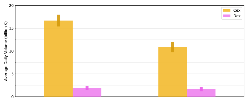
Figure 1: FTX Bankruptcy. The figure shows the average daily volume of CEXs and DEXs during the two-month periods preceding and following the FTX bankruptcy, filed on November 10th, 2022. The vertical lines represent 95% confidence intervals. The plot shows that CEX average daily volume decreased significantly by 35%, from 16.69 to 10.86 million USD. On the contrary, the 13% decrease in DEX daily volume from 1.88 to 1.63 million USD is not statistically significant.

Our research highlights three main issues: First, while cryptocurrency traders benefit from the advantages of LOB efficiency deployed in CEXs, they are exposed to unique types of risk. These encompass custodian risk and potential mismanagement of client funds. To provide visual evidence on the material implications of such risks, Figure 1 shows the sharp decrease in CEX trading volumes in both absolute and relative (to DEXs) terms in reaction to the collapse of FTX, which was one of the largest LOB-based CEXs for cryptocurrency. Second, we quantify market liquidity by conducting a thorough empirical analysis of transaction costs. We show that DEXs operate with similar transaction costs to CEXs, and recent innovations have further reduced DEX transaction costs, making them highly competitive. Third, we assess price efficiency by analyzing deviations from the law of one price implied by the triangular no-arbitrage condition. Despite recent improvements, we find that DEX prices are significantly less efficient than CEX prices. This is due to the crucial role of gas fees in restoring no-arbitrage conditions, reflecting the cost of recording every transaction on the blockchain.

While academic research on the topic is growing fast, we are the first to quantitatively assess the market quality of DEXs, which is important for at least two reasons. First, DEXs represent a novel market structure that could, in the future, be applied to traditional financial securities. By studying the unique characteristics of DEXs, we can identify potential solutions to improve the quality of conventional markets, including those based on the LOB system. For instance, the fact that DEXs rely on AMM rather than LOB has at least three important implications: (i) Regarding market participation, anyone, no matter who they are and what degree of sophistication they have, has the option to offer liquidity to the exchange in a passive fashion through liquidity pools. (ii) Regarding welfare distribution, transaction fees are redistributed between market participants rather than collected by the exchange. (iii) Regarding risk, the custody of assets remains entirely with the user, thus ensuring the highest level of security and censorship resistance. Second, political discourse has primarily focused on the imperative need for regulatory measures within the realm of cryptocurrency markets, with the aim to provide safeguard measures for users and uphold financial stability. This issue is particularly relevant, given the severe market corrections cryptocurrency experienced in 2022. A thorough analysis of the quality of DEXs is desirable so as to address these issues properly.

We proceed in three steps. First, we outline the crucial aspects of trading in CEX and DEX markets, breaking down the components of transaction costs (exchange fees, bid-ask spreads, and gas fees), and point out that delegating the custody of crypto-assets to a CEX involves risk (e.g., hacking and bankruptcy risk) and settlement issues, while DEX users keep their assets in non-custodial wallets. The collapse of FTX gives us an ideal laboratory to analyze the effects of these risks. A difference-in-differences analysis reveals that trading volume on CEXs has significantly decreased while remaining essentially stable on DEXs. This indicates that the realization of such risks led to an erosion of trust in CEXs. Next, we describe the trade-off faced by liquidity providers (LPs) in DEXs, that is, the remuneration earned from exchange fees and the risk of incurring what is known as impermanent loss (IL; also referred to as divergence loss), the AMM analog to adverse selection cost in LOB markets. We also discuss the structural features of DEXs, including the innovations recently brought by the new version of Uniswap v3, which offers a Multiple Fee Tiering (MFT) system and Discretionary Price Ranges (DPR). The MFT system grants LPs the autonomy to determine the transaction fees for which they will be compensated. Concurrently, the DPR mechanism enables LPs to designate the specific price ranges within which they allocate their liquidity, effectively controlling their capital leverage.

The second step is to assess market liquidity by examining transaction costs in CEXs and DEXs. To do this, we investigate a unique and very granular data set that comprises three elements: (i) high-frequency LOB snapshots for two of the most liquid centralized crypto exchanges (Binance and Kraken), (ii) liquidity pool levels and transaction fees for the most prominent DEXs (Uniswap v2, and Uniswap v3), and (iii) historical gas prices for the Ethereum blockchain, computed as the median gas price over the transactions contained in each validated block. This rich information allows us to accurately reconstruct quoted prices and all main transaction cost components for a representative set of exchange pairs of cryptocurrencies. For CEXs, we measure transaction costs as the volume-weighted quoted half-spread based on the available limit orders plus the percentage transaction fees charged by the exchange. Furthermore, we consider that the settlement of a CEX trade involves withdrawal fees charged by the exchange and deposit costs in the form of gas fees paid to miners. For DEXs, we consider the sum of the quoted half-spread (based on the available liquidity in the pools), the percentage transaction fees charged by the protocol and the gas fees paid to miners operating the Ethereum blockchain.

Two main findings stand out: First, DEXs generally feature similar total transaction costs to CEXs. For example, the total transaction costs of trading $100,000\$$ in one of the exchange pairs we study, range from $40\$$ to $67\$$, from $13\$$ to $68\$$, and from $39\$$ to $80\$$ in Uniswap v2, Binance, and Kraken, respectively. Importantly, our difference-in-differences analysis centered on the introduction of Uniswap v3 provides causal evidence that the most recent DEX system considerably reduces DEX transaction costs. For the same amount and pairs above, Uniswap v3 trading costs range from $9\$$ to $52\$$. Our analysis indicates that the MFT system represents the most significant contribution to lowering trading costs. For stablecoin pairs, transaction costs additionally benefit from the DPR system. Second, the analysis of the cost components shows that exchange and gas fees weigh relatively heavily on DEX’s total transaction costs, making DEX costs less predictable.

As the final step, we study price efficiency by examining “triangular” price deviations, that is, the difference between the price of exchanging one currency for another directly (e.g., buying USDC against ETH) and the “synthetic” price that replicates this position by switching from another currency, implying two additional trades (e.g., selling ETH for USDT and then selling the latter to obtain USDC). In addition to being nearly risk-free, this arbitrage condition is the ideal metric for comparing exchanges, as it captures the unique frictions within each market, rather than across multiple markets or related to other instruments like interest rates and FX derivatives, as is the case with the covered interest rate parity condition. Our empirical analysis of exchange triplets uncovers that no-arbitrage conditions are violated more prominently in DEXs. Our results also show that the deployment of Uniswap v3 has improved DEX price efficiency by roughly two-thirds. Despite this substantial improvement, price deviations remain significantly higher than those observed on CEXs. This discrepancy is primarily driven by the pronounced impact of gas fees on transaction costs and arbitrage activity.

The rest of the paper is organized as follows. Section III introduces CEX and DEX systems and a simple mathematical treatment of AMM markets. Section IV describes our dataset and provides some preliminary results. Section V analyses transaction costs. Section VI studies triangular price deviations. Section VII concludes.

II.   Related Literature

We contribute to the nascent but growing literature on cryptocurrencies by providing a comprehensive analysis of two main dimensions of market quality: price efficiency and market liquidity. Concerning price efficiency, prior research provides evidence against it, focusing on Bitcoin. For instance, Makarov and Schoar, (2020) analyzes trading activity and arbitrage deviations using tick data for 34 exchanges across 19 countries. They find arbitrage deviations of Bitcoin prices that are (i) large, persistent, and recurring, (ii) different across countries and regions, and (iii) demand-driven. Krückeberg and Scholz, (2020) provide a detailed analysis of arbitrage spreads among global Bitcoin markets and show that arbitrage spreads concentrate during certain periods, such as the early hours of the day and for new exchange market entries. Hautsch et al., (2018) stress that consensus protocols generate settlement latency, exposing arbitrageurs to price risk. Our contribution is to provide a systematic analysis of price efficiency by studying the triangular no-arbitrage conditions based on a unique and comprehensive set of cryptocurrency triplets traded on CEXs and DEXs.

Regarding market liquidity, Brauneis et al., (2021) perform a horse-race comparison among low-frequency transactions-based liquidity measures. A few other studies use LOB data to study the market liquidity of cryptocurrencies. For instance, Marshall et al., (2019) find that Bitcoin endures substantial variation in liquidity across different exchanges. Considering daily data on Bitcoin prices from 109 exchanges, Borri and Shakhnov, (2018) show that temporal variation of Bitcoin returns increases with illiquidity. We add to the literature by studying liquidity in centralized and decentralized crypto exchanges.

Finally, we contribute to the new literature on decentralized exchanges. So far, theoretical studies have primarily focused on DEXs based on constant-function automated market makers akin to Uniswap v2 (e.g., Angeris et al., , 2019; Capponi and Jia, , 2021; Evans, , 2020; Evans et al., , 2021; Hasbrouck et al., , 2022; Lehar and Parlour, , 2021; Park, , 2021). Among them, Aoyagi and Ito, (2021) examine the conditions for the coexistence of such CEX and DEX exchanges. Rather than the trader’s endogenous choice between CEX and DEX trading venues as in Aoyagi and Ito, (2021), we empirically assess the market quality of DEX and CEX, thus analyzing the coexistence of DEXs and CEXs in equilibrium. Some more recent work also considers DEXs allowing LPs to set DPR or range orders akin to Uniswap v3 (e.g., Lehar et al., , 2023; Heimbach et al., , 2022). On the empirical side, the work of Lehar and Parlour, (2021) compares Uniswap v2 and Binance. Regarding Uniswap v3, Lehar et al., (2023) document fragmented liquidity in the sense that large LPs prevail in high-fee pools while small LPs populate low-fee pools. To avoid the burden of gas fees for each update, Caparros et al., (2023) show that LPs reposition themselves in less costly trading environments (e.g., Polygon).

To sum up, we add to the literature by jointly analyzing multiple CEXs and DEXs. For each exchange, we carry out a comprehensive analysis of the three transaction cost components (i.e., exchange fees, bid-ask spreads, and gas fees) and price efficiency measured as triangular arbitrage deviations. The main message of our study is that the DEX system represents a viable and competitive microstructure.

III.   AMM Markets

A.   High-level description of AMM Markets

Contemporary financial markets primarily employ a central LOB system, wherein a central institution records buy and sell orders, with market prices set by the latest matched orders. The main advantage of the LOB systems is the ability to provide a transparent and efficient price discovery process and liquidity clustering even in extreme situations (Glosten, , 1994). However, implementing a LOB exchange on the blockchain is challenging due to the costly and slow validation process, gas fees, and limited throughput – a crucial resource for order-based exchanges. Crypto exchanges like Binance or Kraken, which use LOB mechanisms, are thus forced to operate off-chain as centralized entities, sacrificing the benefits of decentralized networks.

In contrast, AMMs use an algorithm to establish transaction and market prices based on liquidity provided by participants, relying on a conservation function. The predominant conservation function, known as constant product, mandates that the product of the available liquidity for the two currencies, $x$ and $y$, remains constant. In AMMs, such liquidity is provided by liquidity providers (LPs) who deposit assets into a smart contract representing a specific currency pair’s liquidity pool. Thanks to the conservation function, these reserves establish the assets’ relative price, enabling users to trade without interacting with a third party. A trade on a DEX is also referred to as a swap transaction. To encourage users to supply liquidity to the pools, LPs earn exchange fees from each swap transaction. These fees are equal to 30 basis points of the traded amount for Uniswap v2, while are variable for Uniswap v3 as discussed in Section B.2. More precisely, each LP is rewarded with a fraction of the fee proceeds proportional to the share of liquidity she owns. However, providing liquidity also carries risks. Price divergence between provision and withdrawal can cause economic loss, as LPs receive more of the depreciating asset and less of the appreciating one. The impermanent loss represents the relative loss compared to the holding return, gross of transaction fee revenues. Such risk is akin to adverse selection faced by market makers in markets with information asymmetry, where losses occur only when flows generate a permanent price impact.

We now discuss the main advantages and inconveniences of DEXs compared to order-book-based CEXs, which boil down to a user’s trade-off between retaining control over funds and benefiting from LOB operational efficiency. Indeed, an important drawback of CEXs is that traders have to deposit their crypto assets into the exchange to trade. Deposits and withdrawals are costly, as they are associated with fees charged by the exchange, and gas costs required to submit the transaction to the blockchain. Further, to lower the risk of potential double-spending attacks, exchanges require several block confirmations (12 on Binance and 20 on Kraken) for deposits to be accepted, leading to delays of two to four minutes. Moreover, since CEXs are not tightly regulated, another risk that has arisen in informal discussions with crypto-asset investors is that the CEX operators themselves engage in arbitrage activities by leveraging their privileged position and inside information. Finally, if exchanges mix their own funds with user funds, this exposes clients to bankruptcy risk.

On DEXs, instead, the custody of assets remains fully with the user, as no third party is required to execute the trade. This benefit arising from the decentralized trust provided by blockchain technology has several important implications. First, users can take full advantage of the censorship-resistant and trustless nature of their crypto assets (Pagnotta and Buraschi, , 2018). Second, it allows users to make use of their crypto assets in a variety of protocols and to benefit from their utilities. Third, it neutralizes the risk of hackers attacking the exchange and stealing assets. Fourth, it allows users to save on the fees commonly associated with depositing and withdrawing assets in CEXs. Finally, but very importantly, in DEXs trade and settlement coincide.

Another major innovation brought by DEXs is that their users have the option of passive liquidity provision. This renders the market fairer, given that anyone can provide liquidity, including agents with any degree of sophistication and level of endowment (Lehar et al., , 2023), and does not necessarily require investing in expensive hardware or developing complex algorithms. By contrast, in LOB-based exchanges, LPs are usually highly specialized, and entry costs are high in terms of both sophistication and capital. Market makers need high-speed computers and state-of-the-art algorithms to update their quotes as quickly as possible and avoid being picked off by high-frequency traders (Foucault et al., , 2017).

The DEX market design implies that platform fees charged to each transaction are distributed to LPs in proportion to their shares (Adams et al., , 2020). There is thus no welfare reduction stemming from profits accrued by the exchange itself, as there is no limited liability company associated with it. This may translate into economically significant gains for both traders and LPs.

In DEXs, the market can rapidly adapt and evolve according to participants’ needs. Users can instantly quote any pair of ERC20 tokens without screening procedures. As a result, new tokens tend to become tradeable sooner on DEXs, while CEX approval processes can be time-consuming. Moreover, DEXs may enable trading tokens unavailable on CEXs. This advantage expands investment opportunities, enhances diversification, and accelerates market completeness. However, it also exposes users to potentially malicious assets.

Finally, since DEX transactions are processed by smart contracts and directly recorded on the blockchain, users bear the non-trivial cost of gas fees required to compensate miners. This fact implies that transactions are subject to an execution delay, the duration of which depends on the speed of the underlying blockchain, the chosen gas price, and the level of network congestion. It is important to highlight, however, that for DEX trades, execution and settlement coincide, meanwhile, trades on CEXs cannot be considered settled as long as the funds are inside the exchange. Thus, if settlement issues are taken into account, trading on CEXs involves even higher fees, longer delays, and risks.

B.   Mathematical Foundations of AMM Markets

During both our sample period and at the time of writing, the majority of AMMs relied on the constant product rule, which enables an algebraic determination of market price and transaction price based on the available reserves (Adams et al., , 2021). The leading example is Uniswap, developed and deployed on November 2018 by Hayden Adams, a former mechanical engineer at Siemens. In subsequent sections, we first offer a concise overview of the math underpinning pure constant-product AMMs, which underlines Uniswap v2, Sushiswap, Pancakeswap, and numerous other DEXs. Next, we outline the functioning of the more recent Uniswap v3, which can be viewed as a generalization of the former. Finally, we introduce and formalize the concept of impermanent loss.

B.1.   Uniswap v2

Let $X$ and $Y$ be two crypto tokens. Consider the exchange pair $X\leftrightarrow Y$, and the associated liquidity pool containing $x$ units of $X$ and $y$ units of $Y$. The amount of tokens in the pool determines the current market price $P_{XY}$ of $X$ in terms of $Y$ and its inverse $P_{YX}$, which can be expressed as

$$P_{XY}=\frac{y}{x}\qquad\text{and}\qquad P_{YX}=\frac{x}{y}$$ (1)

Let us denote as $f$ the percentage exchange fees charged by the DEX, and let $\varphi=1-f$. These fees are immediately applied to the traded amount $\Delta x>0$, so that the net quantity of token $X$ that goes into the swap transaction is $\varphi\Delta x$. Each trade (swap transaction) is automatically regulated by the constant product rule, which states that the product of the reserves must remain constant before and after any transaction. Hence, when trading an amount $\Delta x>0$ of token $X$ in exchange for token $Y$, the output quantity $\Delta y$ is mathematically determined by the following equation

$$xy=k=(x+\varphi\Delta x)(y-\Delta y)\;,$$

where $k$ is the constant product invariant. Solving for $\Delta y$, one obtains that the output amount is given by

$$\Delta y=y\frac{\varphi\Delta x}{x+\varphi\Delta x}.$$ (2)

The transaction price is, therefore, lower than the quoted price and is given by

$$T_{XY}(\Delta x)\;=\;\frac{\Delta y}{\varphi\Delta x}\;=\;\frac{y}{x+\varphi\Delta x}$$

and the quoted half-spread (as a percentage of the quoted price) can be computed as

$$S_{XY}(\Delta x)=\frac{P_{XY}-T_{XY}}{P_{XY}}=\frac{\varphi\Delta x}{x+\varphi\Delta x}\;.$$ (3)

Note that the above is an increasing but concave function of the transaction volume $\Delta x$, implying that larger volumes have a larger impact on prices but with a marginally decreasing effect. Ceteris paribus, a purchase could have a greater impact than a sale, as showed in Aoyagi and Ito, (2021). Throughout the paper, we compute the quoted half-spread for both directions ($X\to Y$ and $Y\to X$) for the same traded amount in terms of dollars and consider the average of the two measures. In the following, we refer to this metric as Bid/Ask Spread or B/A Spread for short.

B.2.   Uniswap v3

Uniswap v3, released on May 5th, 2021, is based on a generalization of the constant-product AMM model. The upgrade, deployed through a new set of smart contracts, includes two innovations that are highly relevant to our market quality analysis, namely: (i) the Multiple Fee Tiering (MFT) system, that is, the possibility for LPs to choose the level of exchange fees; (ii) the Discretionary Price Ranges (DPR) system, allowing LPs to post liquidity on a specific price interval.

The MFT system is based on the capability of the new protocol to deploy several liquidity pools for the same exchange pair, each with a different level of exchange fees attached to it. More specifically, the available fee levels – in basis points – have support in the discrete set {1, 5, 30, 100}. This implies, in particular, that there can be at most four liquidity pools for the same exchange pair. LPs are free to decide their allocation of liquidity across pools, and, likewise, traders can decide in which pool they want to trade. Each of those pools works as a standard v2 pool and is independent of its siblings. It is endowed with pool-specific levels of liquidity $x_{f}$ and $y_{f}$, aggregating the liquidity supplied by LPs at fee level $f$. This implies that different pools for the same currency pair may display different quoted prices and Bid/Ask spreads. In equilibrium, however, arbitrage activity should limit price deviations from the law of one price. From a theoretical standpoint, liquidity allocation depends on the risk-return trade-off faced by LPs, as described in the simple model of liquidity provision proposed in Section A of the Internet Appendix. In particular, relevant factors determining the allocation of liquidity across different fee levels should include: (i) the expected volatility of the exchange rate, proportional to the expected impermanent loss. For pairs with a higher expected impermanent loss, LPs should require higher exchange fees as a risk compensation; (ii) the expected trading volume in the pair, proportional to the expected profit from liquidity provision. For pairs with a larger expected volume, LPs should accept lower exchange fees; (iii) the level of liquidity already present in the pool, since less crowded pools provide higher returns on capital to the marginal LP. Further, the allocation of liquidity between high- and low-fee pools may depend on the heterogeneity of capital endowment across LPs, as theorized by Lehar et al., (2023).

MFT can enhance market quality by lowering the effective transaction costs for traders. With the support of Uniswap’s automatic router, traders can select the optimal pool for a specific trade size by balancing the trade-off between Bid/Ask spreads and fees.

The second innovative feature of v3 is DPR, which opens up the possibility for LPs to confine their liquidity provision to a specific price interval, allowing LPs to offer liquidity in a more proactive manner. Technically, the protocol uses a discrete set of price ticks to divide the full price range of a trading pair into a discrete number of intervals. An LP can provide liquidity to a custom range, opening a so-called liquidity position, by specifying the lower and upper ticks in addition to the supplied quantity. Aggregating over all LPs’ positions, one obtains the distribution of liquidity over the entire price range, which can take any arbitrary shape.

To convey some intuition, let us briefly discuss the case of a single liquidity position delimited by two subsequent ticks. Formally, consider a liquidity pool for the exchange pair $X\leftrightarrow Y$ and a liquidity position concentrated on the interval $[P_{a},P_{b}]$. Following Adams et al., (2021), the quantities $\tilde{x}$ and $\tilde{y}$ supplied to the pool are referred to as real reserves. Let $x$ and $y$ be the corresponding virtual reserves, defined on the current interval as

$$x=\tilde{x}+L/\sqrt{P_{b}}\qquad\text{and}\qquad y=\tilde{y}+L\sqrt{P_{a}}$$ (4)

where $L=\sqrt{xy}$ is referred to as the virtual liquidity attached to the interval. Locally on the interval, all relevant quantities are defined similarly as in Uniswap v2, but in terms of virtual reserves rather than real reserves. In particular, the quoted price is $P=y/x$, and the constant product rule reads $xy=k$.

In other words, when a swap transaction occurs within a single price interval, the pricing rule is exactly the same as in Uniswap v2, driven by the constant-product formula applied to the virtual liquidity available on that interval. If the price impact of the trade pushes the quoted price across one or multiple ticks, the constant-product formula applies locally based on the virtual liquidity attached to each interval.

The exchange fees collected on each interval are divided among LPs based on the share of liquidity they deposited in that specific interval. In particular, a liquidity position earns fees only if swap transactions are performed on its support. The DPR system aims at reducing transaction costs mainly for stable-coins pairs, enjoying very low levels of exchange-rate volatility. For instance, on the USDC-USDT pair, where both stablecoins are pegged to the US dollar, LPs are incentivized to concentrate their liquidity within a few intervals around the price of $1$, thus leading to lower Bid/Ask spreads in that region.

The Bid/Ask spread formula for Uniswap v3 is less straightforward than its v2 counterpart, described in (3), as it depends on the liquidity distribution across price intervals. To derive it, consider a liquidity pool for the exchange pair $X\leftrightarrow Y$ with quoted price $P$. Assume the trade size is $\Delta x$ and denote by $P^{\prime}$ the final quoted price after the transaction. Let us start with the simple case where a trade of size $\Delta x$ is fully executed within a single price interval. To make the notation lighter, we ignore exchange fees in this derivation. Recall that the liquidity of the interval is $L=\sqrt{xy}$, where $(x,y)$ are the virtual reserves for the interval before the trade, and $(x^{\prime},y^{\prime})$ denote the virtual reserves after the trade. Since $L$ is invariant to trades, we have

$$x=L/\sqrt{P},\qquad y=L\sqrt{P},\qquad x^{\prime}=L/\sqrt{P^{\prime}},\qquad y^{\prime}=L\sqrt{P^{\prime}}.$$ (5)

It thus follows that the relationships between $\Delta x$, $\Delta y$, and the quoted prices are

$$\Delta x=L\left(1/\sqrt{P^{\prime}}-1/\sqrt{P}\right)\qquad\text{and}\qquad\Delta y=L\left(\sqrt{P}-\sqrt{P^{\prime}}\right)$$ (6)

The transaction price can therefore be written as $\Delta y/\Delta x=\sqrt{PP^{\prime}}$, showing that it equals the geometric mean of $P$ and $P^{\prime}$.

To derive a general expression for the transaction price in the case of a trade spanning multiple intervals, define the price intervals $I_{t}=[P_{t},P_{t-1}]$ for $t\in\mathbb{Z}$ such that $P\in I_{0}$ and let $\tau$ be a positive integer such that $P^{\prime}\in I_{\tau}$. Further, let $\Delta x_{t}$ denote the amount traded within $I_{t}$, and let $T_{t}$ be the corresponding transaction price. The effective transaction price can thus be written as the volume-weighted average of the local transaction prices for each of the relevant intervals as a function of the trade size and the distribution of liquidity:

$$T = \frac{1}{\Delta x}\left[\Delta x_{0}T_{0}+\sum_{t=1}^{\tau-1}\Delta x_{t}T_{t}+\Delta x_{\tau}T_{\tau}\right]$$ (7)

$$= \frac{1}{\Delta x}\left[L_{0}\left(\sqrt{P}-\sqrt{P_{0}}\right)+\sum_{t=1}^{\tau-1}L_{t}\left(\sqrt{P_{t-1}}-\sqrt{P_{t}}\right)+L_{\tau}\left(\sqrt{P_{\tau-1}}-\sqrt{P^{\prime}}\right)\right]$$ (8)

Finally, the spread equals the percentage deviation from the quoted price, that is

$$S_{XY}(\Delta x)=\frac{P-T}{P}$$ (9)

B.3.   Impermanent Loss

Similarly to liquidity provision in LOB markets, providing liquidity to AMM-based DEXs involves a trade-off between expected profits and adverse selection risk. On the one hand, LPs are compensated by pocketing the transaction fees applied to the trading volume generated by liquidity takers through swaps. On the other hand, a permanent price change leads to an impermanent loss (IL) for the LP. This loss arises from the fact that, gross of fees, providing funds to a liquidity pool is less profitable than simply holding the tokens (Loesch et al., , 2021). In the following, we derive a mathematical expression for the IL in Uniswap v2, followed by a brief discussion of the same issue in the context of Uniswap v3.

Consider a liquidity pool on Uniswap v2 for the exchange pair $X\leftrightarrow Y$, containing $x$ and $y$ units of the two tokens at time $t=0$. Assume an LP owns a share $\psi$ of the pool, and the current quoted price is $P=y/x$. At $t=0$, the value of her position in units of $y$ is $W=\psi(xP+y)=2\psi y$. Denote the new reserves at $t=1$ as $(x^{\prime},y^{\prime})$ and the new price as $P^{\prime}$, so that the value of her position in units of $y$ changes to $W^{\prime}=\psi(x^{\prime}P^{\prime}+y^{\prime})=2\psi y^{\prime}$. The gross percentage change in the value of the deposited liquidity can therefore be expressed as $R_{LP}=W^{\prime}/W=y^{\prime}/y$. Given the constant product rule $xy=k=x^{\prime}y^{\prime}$ and the definition of the quoted price, we can write $y=\sqrt{kP}$ and $y^{\prime}=\sqrt{kP^{\prime}}\,.$ Hence, the change in value of the LP’s liquidity position depends solely on the square root of the gross price change $\Delta P=P^{\prime}/P$ between $t=0$ and $t=1$:

$$R_{LP}=\frac{y^{\prime}}{y}=\frac{\sqrt{kP^{\prime}}}{\sqrt{kP}}=\sqrt{\Delta P}\,.$$

On the other hand, the gross return $R_{H}$ from holding the tokens is simply the average of the returns arising from holding each individual token. This equals to $1$ for $Y$ – the accounting unit – and $\Delta P$ for $X$. The total holding return is thus

$$R_{H}=\frac{1}{2}(\Delta P+1)\,.$$

The impermanent loss, that is, the net opportunity cost from providing liquidity in Uniswap v2 instead of holding the tokens, is therefore given by

$$IL_{2}=R_{H}-R_{LP}=\frac{1}{2}\left(\Delta P+1\right)-\sqrt{\Delta P}\,.$$ (10)

By taking the first order derivative with respect to $\Delta P$, one can easily see that $IL$ has a global minimum of $0$ for $\Delta P=1$, while it is strictly positive otherwise. Hence $IL$ represents a cost and highlights that, gross of pocketing the fees, LPs providing liquidity are always worse off than token holders. We note that $IL$ can be seen as a measure of the level of adverse selection faced by LPs, similar to that faced by market makers in LOB markets. In fact, for any given horizon, $IL=0$ if the order flow is uninformed and gives only rise to a temporary price impact ($\Delta P=1$), while it increases in magnitude in the presence of informed order flow, causing a permanent price change ($\Delta P\neq 1$). Intuitively, the provision of liquidity in the AMM framework can be remunerative if the LP provides immediacy primarily to liquidity traders while, at the same time, it may involve net losses when facing a higher fraction of informed traders. Quantitatively, Fukasawa et al., (2022) show that the IL in constant-product AMMs can be hedged through weighted variance swaps.

The introduction of the DPR system in Uniswap v3 complicates the calculation of IL for a liquidity position, as it hinges on the position’s price range. Although a comprehensive discussion is beyond this paper’s scope, we provide a derivation of IL in a special case, assuming liquidity is provided on a single interval centered on the quoted price and that the final price stays in the interval. Formally, consider a liquidity position on the interval $[P_{a},P_{b}]$, with virtual reserves $(x,y)$ corresponding to real reserves $(\tilde{x},\tilde{y})$. Assume the initial quoted price $P_{0}$ equals the geometric mean of the interval so that the dollar value of the real reserves is balanced. It follows that the initial value of the position in units of $Y$ is given by $W=\tilde{x}P+\tilde{y}=2\tilde{y}$ and the $t=1$ value resulting from holding the two tokens is $W_{H}^{\prime}=\tilde{x}P^{\prime}+\tilde{y}=(1+\Delta P)\tilde{y}.$ Hence, the return from holding the tokens is $R^{H}=(1+\Delta P)/2$, as in Uniswap v2. Assuming the new price $P^{\prime}$ does not exit the interval, we can easily find the new real reserves ($\tilde{x}^{\prime},\tilde{y}^{\prime}$) and the resulting value of the liquidity position at $t=1$, which is given by $W_{LP}^{\prime}=\tilde{x}^{\prime}P^{\prime}+\tilde{y}^{\prime}.$ Applying the constant product rule to virtual reserves and transforming them back to real reserves, using the relation expressed in (4), we get

$$\tilde{x}^{\prime}=L(1/\sqrt{P^{\prime}}-1/\sqrt{P_{b}})\qquad\text{and}\qquad\tilde{y}^{\prime}=L(\sqrt{P^{\prime}}-\sqrt{P_{a}}).$$ (11)

Similarly, the initial value of the position can be re-written as $2\tilde{y}_{0}=2L(\sqrt{P_{0}}-\sqrt{P_{a}})$. Hence, with some algebraic manipulations, IL in Uniswap v3 can be expressed as

$$IL_{3} = R^{H}-R^{LP}=\frac{(1+\Delta P)}{2}-\frac{\tilde{x}^{\prime}P^{\prime}+\tilde{y}^{\prime}}{2\tilde{y}}$$ (12a)

$$= \frac{(1+\Delta P)}{2}-\frac{L(2\sqrt{P^{\prime}}-(1+\Delta P)\sqrt{P_{a}})}{2L(\sqrt{P}-\sqrt{P_{a}})}$$ (12b)

$$= \frac{\sqrt{P}}{\sqrt{P}-\sqrt{P_{a}}}\left(\frac{1}{2}\left(\Delta P+1\right)-\sqrt{\Delta P}\right)$$ (12c)

$$= \lambda\,IL_{2}$$ (12d)

where $\lambda=\sqrt{P}/(\sqrt{P}-\sqrt{P_{a}})$ can be interpreted as a leverage factor that increases as the interval narrows. Note that the impermanent loss in Uniswap v3 converges to that of Uniswap v2 if the interval covers the entire price range and $\lambda\to 1$. In summary, the introduction of the DPR system in Uniswap v3 opens the possibility for LPs to take leveraged liquidity position, where both the earned exchange fees and the IL are increasing in the leverage factor.

IV.   Data and Preliminary Results

Because DEXs are based on smart contracts deployed on blockchains, records of every interaction with those contracts are available to the public. This rich dataset includes, as primitives, the creation of exchange pairs, the addition and removal of liquidity by LPs, and swap transactions between two quoted tokens. Building on those, one can reconstruct liquidity levels, quoted prices, transaction prices, and trading volume at the pair level at any time. We leverage the application programming interface of TheGraph.com, an indexing protocol enabling efficient querying of data from blockchains, to obtain data for Uniswap v2 from the Ethereum Mainnet. Equivalent data regarding Uniswap v3 is collected using custom queries on Dune.com, a community-driven platform that facilitates querying of public blockchain data. For CEXs, by contrast, data are proprietary. We obtain minute-frequency full LOB snapshots and Open, High, Low, Close, and Volume data from Kaiko, a data provider specialized in cryptocurrencies, for all pairs quoted on the highest-volume crypto exchanges, such as Binance International and Kraken. For both CEXs and DEXs, our sample period spans from March 2021 to February 2023. Specifically, Uniswap v2 data ends in February 2022, while Uniswap v3 data is available from its introduction, in May 2021, to February 2023. For our main empirical analysis of market quality, we focus on five of the most liquid and traded cryptocurrency pairs. To select these pairs, we first consider the intersection of trading pairs present in Uniswap v2, Binance, and Kraken at the beginning of our sample. We then compute percentile rankings of average daily volumes in USD over our sample period on each of the three exchanges and take their average. Finally, we select the first five pairs ranked by the resulting metric.

There are two important moments during our sample period that allow us to carry out insightful difference-in-differences analyses. The first event is the collapse, on November 10th, 2022, of FTX, one of the largest LOB-based centralized exchanges for cryptocurrency. The bankruptcy was triggered by a liquidity crisis pertaining to the exchange’s proprietary token, FTT, and led to significant market volatility and multibillion-dollar losses. Some evidence suggests the misuse of its clients’ assets. Specifically, it has been reported that FTX allocated $10 billion from its client accounts to bolster Alameda Research, a cryptocurrency trading entity operated by Sam Bankman-Fried, who is also the founder of FTX. Such an action contravenes the stipulated terms of service of FTX, which explicitly maintain that clients’ funds should not be appropriated for purposes beyond trading on the FTX platform. Furthermore, allegations have emerged contending that FTX employed a Ponzi-like scheme to misappropriate funds, involving the transfer of customer resources among different entities. These claims, if substantiated, highlight a serious breach of fiduciary duty, underscoring the custody risks associated with centralized cryptocurrency exchanges. Hence, this event provides us with an ideal laboratory to analyze the effects of custodian risks embedded in LOB-based CEX markets. The second event is the inception of Uniswap v3 which occurred on May 5th, 2021. This event allows us to compare the market quality of the new Uniswap v3 and its previous iteration, v2, and that of CEX markets.

A.   Trading Volume

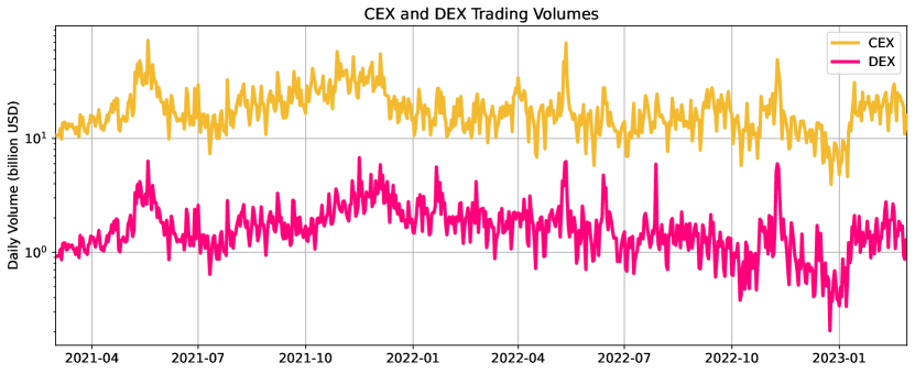
Figure 3: Aggregate Trading Volume. The figure presents aggregate traded volumes for the CEXs (Binance, and Kraken) and DEXs (Uniswap v2, and Uniswap v3) in our sample. from March 2021 to February 2023. The plotted volume is the aggregate trading volume across all listed pairs, including those not appearing in our main analysis. The vertical axes use the log scale and are expressed in million USD.

Figure 3 showcases the cumulative traded volumes for the CEXs (Binance and Kraken) and DEXs (Uniswap v2 and Uniswap v3) included in our sample, expressed in billion USD. The data reveals two main patterns: First, while a temporary drop following the collapse of FTX at the end of 2022 is visible, the trading volume for both CEXs and DEXs has generally remained relatively steady. Second, trading volumes in CEXs are approximately 10 times larger than those in DEXs throughout the period. Table II presents the daily average trading volume for the pairs we consider in millions of USD, broken down by exchange. These pairs provide a representative sample, as they generate between $14\%$ and $33\%$ of the volume on each exchange. Figure 5 presents the distribution of trade sizes for swap transactions executed in Uniswap v2 and Uniswap v3 based on blockchain data, while we do not have access to the equivalent information from CEXs. The histogram reveals that the bulk of trades ranges between $1$ and 10,000 USD, accounting for approximately $70\%$ of all recorded transactions. Yet, there are instances of significantly large trades surpassing $1$ million USD, making up for $0.5\%$ of the observations.

B.   Self-Custody and FTX Collapse

The collapse of FTX gives us an ideal laboratory to analyze the effects of the risks in granting centralized exchanges the custody of assets, discussed in Section III. FTX was one of the world’s largest cryptocurrency exchanges. It filed for bankruptcy on November 11, 2022, jeopardizing around $740\$$ million worth of crypto assets deposited on the FTX platform (Huang, , 2022). We posit that this event may have triggered an erosion of trust due to the increased saliency of deposit risks and mismanagement of users’ assets by CEX system operators. The hypothesis we test is whether the FTX downfall has decreased trading volumes in other CEX markets (like Binance and Kraken) relative to DEXs. In addition, a simultaneous increase (decrease) in trading volumes on DEXs would suggest a substitution (negative spill-over) effect from CEXs to DEXs.

To test these hypotheses, we perform difference-in-differences regression analyses of the trading activity on CEX and DEX exchanges around the time when FTX filed for bankruptcy. The sample encompasses a period of two months before (September 9, 2022) and after (January 9, 2023) the event. The dependent variable is the daily trading volume (both in billion US Dollars and in logarithm terms) on CEXs (Binance and Kraken) and DEXs (Uniswap v2 and v3), which is regressed on a treatment dummy (DEX) indicating DEXs, a time dummy (FTX) indicating the period after the FTX collapse, and their interaction. We check and confirm the validity of the parallel trend assumption.

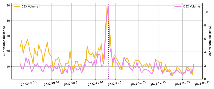
Figure 2: FTX Event Study. The figure displays the time-series evolution of daily trading volumes on CEXs (Binance and Kraken) and DEXs (Uniswap v2 and Uniswap v3), around the collapse of the FTX exchange on November 10th, 2022 (depicted by a dotted vertical line). The CEX trading volume is measured on the left axis, while DEX volume is measured on the right axis. Both series are presented in billion US Dollars.

The time series evolution of aggregate trading volumes on CEXs and DEXs in Figure 2 clearly illustrates a sharp decrease in CEX volumes. The regression results reported in Table VII shed more light on what happened in reaction to that event, indicating a significant collapse in trading volumes on CEXs and a stable holding of volumes on DEXs. Thus, these findings suggest that CEX’s users reacted to the materialization of risks inherent in centralized systems, reducing the trading volume allocated to CEXs in the two months following the FTX bankruptcy. In contrast, DEX transaction volumes remained stable, discarding the idea of positive or negative spill-over effects.

C.   Gas Prices

The term gas refers to the unit of measure of the computational effort required to execute transactions on the Ethereum network. The aggregate gas fees for a given block, summing over all transactions, are paid in the network’s native currency (ETH for Ethereum) and collected by the miner validating the block. To trade on a DEX, as for any on-chain transaction, more generally, the user has to pay a number of gas units proportional to the computational complexity of the transaction. The resulting dollar cost is the product between the units of gas used and the gas price, which the user can choose to control the priority of execution. Miners select, among the set of pending transactions, those to include in the new block, prioritizing the most profitable transactions, that is, those with the highest gas price. Wallet interfaces automatically suggest an optimal gas price, depending on the current level of network activity and based on the trade-off between the probability of execution within the next few blocks and the cost. While users can edit the gas price according to their preferences, our data reveals that most transactions are executed at the median gas price of the block.

Gas costs are undoubtedly important in the study of trading in fully decentralized AMM markets since all interactions are on-chain. Every trade is triggered by a transaction submitted by the user to the blockchain, representing a function call on the protocol’s smart contracts. Further, on closer inspection, gas fees also matter in CEX trading. In fact, a CEX-based trade is only settled when the trader transfers the asset from the exchange wallet back to her non-custodial wallet. The settlement process thus involves the gas fees paid to miners for the deposit of funds (“deposit fees”) and fees charged by the exchange for the withdrawal (“withdraw fees”). The transaction representing the deposit is executed by the user, who has to pay the gas directly to the network, while the withdrawal operation is executed by the exchange, which pays for the gas and requires compensation from the user.

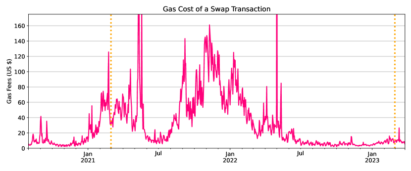
Figure 4: Gas Fees. The figure presents the time series evolution of the gas costs of a swap transaction in our sample in USD. This is computed at the hourly frequency, multiplying the units of gas required to execute a swap, numbering roughly 120,000, by the average gas price associated with transactions in the blocks validated during each hour in USD. Since the number of gas units is constant over time, the time series variation comes from oscillating gas prices in ETH and the fluctuation of the USD/ETH exchange rate. The two orange vertical lines indicate the period on which our main market quality analysis is conducted, that is, from the beginning of March 2021 to the end of February 2023.

Figure 4 plots the evolution of the gas fees (in USD) required to execute a swap transaction on Uniswap, equal to the product between gas units and gas price, in USD. The figure is based on an estimate of the gas units required for a swap on Uniswap v2, constant over time, and an estimate of the prevailing gas price on each day. We estimate the former for each pair by sampling swap transactions every 100 blocks over the entire sample period using a local Ethereum node and Infura APIs, resulting in roughly 330,000 transactions. While, in principle, those could vary across specific trading pairs depending on the implementation of the ERC-20 contracts for the two tokens, we empirically find only minor variations across pairs. We hence use the median value of 118,340 gas units for the plot. We separately repeat the estimation for swaps performed on Uniswap v3, based on roughly 200,000 transactions, finding that the required gas amounts are also homogeneous across pairs and roughly $10\%$ more costly with respect to Uniswap v2. Throughout the paper, we use the median values of 118,340 gas units for Uniswap v2 and 130,889 gas units for Uniswap v3. Finally, we estimate the gas price attached to swaps using the above-mentioned set of Uniswap v2 and Uniswap v3 swap transactions by taking the median gas price on an hourly basis.

Since the amount of required gas for such an operation is constant over time, the observed time-series variation arises from two factors: (i) the price of ETH relative to the USD and (ii) the prevailing gas price of the network, depending on the level of network congestion. The series presents substantial variability, ranging from less than $10\$$ in the first part and last part of the sample to $300\$$ between April and May 2022. The two vertical lines mark the period from March 2021 to February 2023, the period in which our primary analysis of market quality is conducted.

V.   Transaction Costs

Now that we possess a comprehensive understanding of the operational mechanisms of CEXs and DEXs, and have access to the relevant data, we can proceed to analyze the first key aspect of market quality - market liquidity. A common definition of market liquidity is the ease with which an asset can be traded at a price close to its consensus value (Foucault et al., , 2013). We employ a widely accepted measure of market illiquidity, that is, the effective transaction cost associated with a single trade. It is expressed as a percentage of the traded amount. Transaction costs account for both the price impact associated with a given trade size and any kind of commissions charged by the protocol or the exchange. Due to their fundamentally different mechanics, CEX and DEX transaction costs are modeled using distinct methodologies. Nevertheless, the two measures are based on the same conceptual framework, as they are meant to capture the effective costs incurred by a trader transacting a given amount (in US Dollar terms), including slippage, fees, and settlement costs.

Empirically, we estimate transaction costs $TC_{XY}(\Delta x)$ for a trade $X\leftrightarrow Y$ at an hourly frequency for the five pairs in our sample and different trade sizes $\Delta x\in(10^{3},10^{4},10^{5},10^{6})$ expressed in USD, separately for DEXs and CEXs.

A.   CEX Transaction Costs

For CEXs based on LOB, we measure transaction costs of a market order of a given dollar amount by considering four distinct components: (i) the Bid/Ask spread implied by the depth of the LOB, (ii) the exchange fees charged by the platform (taker fees), (iii) the gas fees paid to transfer crypto tokens to the exchange, and (iv) withdrawal fees charged by the exchange. The third and fourth components constitute a measure of settlement costs, motivated by the assumption that the trader does not delegate the ownership of its funds to the exchange. Rather, we assume that the trader originally holds the crypto tokens in her non-custodial wallet and transfers token $X$ to the exchange whenever she wants to trade. After the transaction $X\to Y$ occurs inside the exchange, she withdraws the resulting units of the $Y$ token by transferring them back to her wallet. These deposit and withdrawal operations are expensive and will be discussed below.

We start with the Bid/Ask spread associated with a market order which, since we observe the full depth of ask and bid quotes present in the order book at any point in time, can be computed directly using the volume-weighted bid and ask prices. More specifically, we define the volume-weighted bid price $B_{XY}$ for a sell order of size $\Delta x$ as

$$B_{XY}(\Delta x)=\frac{\sum_{i}v_{i}b_{i}}{\Delta x}\qquad\text{such that}\qquad\sum_{i}v_{i}=\Delta x\;,$$

where $v_{i}$ and $b_{i}$ represent the volume and the price of each filled bid limit order $i$, respectively. The volume-weighted ask price $A_{XY}$ for a buy order of size $\Delta x$ is defined symmetrically as

$$A_{XY}(\Delta x)=\frac{\sum_{j}v_{j}a_{j}}{\Delta x}\qquad\text{such that}\qquad\sum_{j}v_{j}=\Delta x\;,$$

where $v_{j}$ and $a_{j}$ represent the volume and the price of each filled ask limit order $j$, respectively. We then define the Bid/Ask spread as

$$S_{XY}(\Delta x)=\frac{A_{XY}(\Delta x)-B_{XY}(\Delta x)}{A_{XY}(\Delta x)+B_{XY}(\Delta x)}\;.$$ (13)

Next, the deposit of funds involves the trader paying an amount of gas fees to submit the transaction on the blockchain. The cost of such an operation is fixed in terms of the required gas units (21,000 for the native token ETH and 65,000 for ERC20 tokens). Its dollar value depends on the prevailing gas price on the network. Consequently, we calculate deposit fees as the product of the gas units needed for the transaction, contingent on whether $X$ is the native currency and the prevailing gas price (in USD) at the trade time. Moreover, withdrawing from the exchange to a personal wallet incurs a fee charged in the withdrawn currency units. We gather these fees for each token of interest from Binance and Kraken, converting them to USD based on the token’s value at the trade time. Finally, we define the total transaction costs by adding up the four components defined above. For the sake of simplicity, we condense the deposit and withdrawal fees into one term $DW_{X,Y}/\Delta x$ representing the entirety of settlement costs as a percentage of the traded amount, while we leave the percentage exchange fees $f$ as a separate entity. We thus have

$$TC_{XY}(\Delta x)=S_{XY}(\Delta x)+f+\frac{DW_{XY}}{\Delta x}\;,$$ (14)

Notice that the first and last terms in the above expression are time-varying, while exchange fees are constant.

B.   DEX Transaction Costs

For DEXs based on AMM, we measure transaction costs of a trade of a given dollar amount by considering three distinct components: (i) the Bid/Ask spread implied by the depth of the liquidity pools; (ii) the exchange fees charged by the exchange; (iii) the gas fees paid to submit the blockchain transaction. As previously explained, the dollar value of gas fees depends on the computational complexity of the smart-contract function being called, the execution priority chosen by the trader, and the prevailing gas price at the execution time. For our purposes, we are interested in the gas required to execute a swap transaction; For instance, in Uniswap v2, this involves invoking the swapExactTokensForTokens function of the relevant router contract. We assume that the quantity of gas required to execute a swap transaction is constant across all currency pairs at $\Gamma=$ 118,340 gas units for Uniswap v2 and 130,889 for Uniswap v3, as discussed in Section C. We then approximate the gas cost $g$ of a swap during each hour of our sample period multiplying $\Gamma$ by the median gas price paid across all Uniswap v2 and Uniswap v3 transactions recorded during that hour in dollar terms.

The transaction costs for Uniswap v2 are thus computed as the sum of the Bid/Ask spread $S_{XY}$, defined in (3) and averaged across both directions $X\to Y$ and $Y\to X$, the constant exchange fee $f=30$ bps for Uniswap v2, and the gas fee $g$ as a fraction of the trade size. When it comes to Uniswap v3 we apply a similar methodology, even though the calculation differs slightly due to the MFT system and the existence of multiple pools for any given exchange pair. Specifically, we compute transaction costs for each pool separately, using the Bid/Ask spread derived in (9), and considering the unique exchange fees of the pool. For each trade size and each hour, we then identify the most cost-effective pool for executing the trade, that is, the one resulting in the lowest overall transaction costs, including gas fees. Our approach considers that traders can effortlessly select the most advantageous pool, since the Uniswap interface, through its router contract, automatically recommends it. Note that, as the optimal pool depends on both the offered fees and the available liquidity, it can vary across different trade sizes and over time. We will assess the degree of such variation empirically in Section V.

Hence, the transaction costs for the two DEXs can be summarized as

$$TC_{XY}(\Delta x)=S_{XY}(\Delta x)+f+\frac{g}{\Delta x}.$$ (15)

As in the CEX case, the first and last terms in the above expression are time-varying. The exchange fees $f$ are constant for Uniswap v2, while in Uniswap v3 they depend on the optimal pool selected, as discussed above.

C.   Descriptive Analyses of Transaction Costs

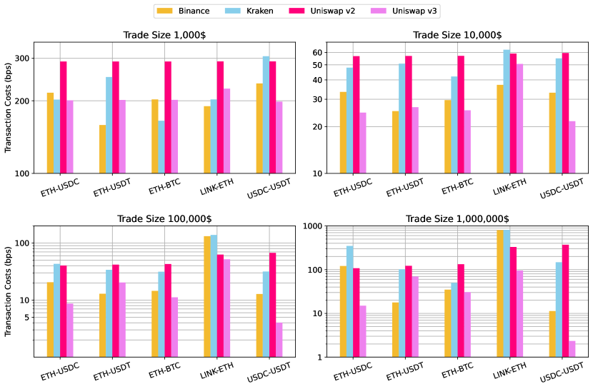
Figure 6: Transaction Costs. The figure presents transaction costs, computed as in equation (14) for the LOB-based Binance and Kraken and on equation (15) for the AMM-based Uniswap v2 and Uniswap v3. The transaction costs are computed at the hourly frequency for the five pairs in our sample and for different trade sizes ($10^{3},10^{4},10^{5}$, and $10^{6}$ US dollars), then averaged from March 2021 to February 2023. As discussed in Section V, the displayed transaction costs include B/A spreads, exchange fees (30 basis points for Uniswap v2, 10 basis points for Binance, and 26 basis points for Kraken), and settlement fees (gas fees for Uniswap v2 and Uniswap v3, and deposit and withdraw fees for the two CEXs). For Uniswap v3, daily and for each trade size, we consider the liquidity pool offering the lowest transaction costs among those available for the specific exchange pair. The vertical axis employs a logarithmic scale and is reported in basis points.

Our analysis begins by examining the average transaction costs (TCs) across different trade sizes on DEXs (Uniswap v2 and v3) and CEXs (Binance and Kraken). The results, presented in Figure 6 , illustrate log TCs calculated at an hourly frequency using equations (15) and (14) and then averaged over the entire sample period. Additionally, Table III offers a detailed breakdown of the total TCs into their three components (bid-ask spread, gas or deposit-withdrawal fees, and exchange fees) across different trade sizes. Finally, Table IV provides statistics on the time-series variance of each cost component, focusing on a $\$10,000$ trade.

Four main findings stand out: First, upon comparing the overall TCs, we find that Uniswap v3 and Binance perform significantly better than Uniswap v2 and Kraken, providing lower TCs for most exchange pairs and trade sizes (19 out of 20). Uniswap v3 performs marginally better than Binance, offering the lowest TCs in 13 out of 20 cases. All in all, these two exchanges offer similar levels of TCs to their users, showing that the leading CEX and DEX are in the same ballpark regarding this dimension of market quality.

Second, Table IV indicates that most of the variability in TCs for a $\$10,000$ trade comes from gas fees (DEXs) and DW fees (CEXs). While Uniswap v3 exhibits variations in the Bid/Ask spread component similar in magnitude to those of Binance, it suffers from a higher sensitivity to gas prices, leading to a significantly higher variation in total TCs. Moreover, the estimates in Table III indicate that costs related to gas fees and DW fees are roughly of the same magnitude across all exchanges, trading pairs, and trade sizes.

Third, as displayed in Figure 6 , there is an observable convexity in the total cost relative to trade size across both DEXs and CEXs for most trading pairs. Total costs peak for smaller transactions ($1,000), drop to their lowest for medium transactions ($10,000 to $100,000), then rise again for larger transactions ($1 million). This pattern aligns with expectations as, according to Table III, gas fees on DEXs represent a substantial proportion of the traded amount for $1,000 transactions. Similarly, deposit and withdrawal fees are the most influential component on CEXs for this trade size, although they are lower in absolute terms. As the size of the transaction increases, however, the exchange fees and gas costs become marginal while the spread plays a more predominant role. When the trade size becomes very large relative to the available liquidity, as for $1 million, spreads become even more pronounced, leading to an increase in TCs.

Fourth, TCs for the stablecoin pair USDT-USDC in Uniswap v3 exhibit a consistent monotonic decrease with trade size, reaching a remarkably low rate of $2$ basis points for a $1 million transaction. Such low cost in traditional financial securities is attributable to the most liquid securities, for example, the EURUSD or USDJPY foreign exchange (FX) rates (see, e.g. Karnaukh et al., , 2015). This competitive figure – significantly lower than $11$ bps on Binance, $147$ on Kraken, and $370$ on Uniswap v2 – can be attributed to the innovative DPR and MFT systems and the stable nature of the assets. Since both tokens are pegged to the US Dollar, the exchange pair volatility is minimal, thereby implying a negligible expected impermanent loss for LPs. Referring to equation (12a), it is logical for LPs to amplify their position by focusing liquidity around the $1$ price point, resulting in extremely narrow spreads for trades around this price. Moreover, the MFT system fosters a reduction of exchange fees for this pair. Indeed, considering the high trading volume and the minimal expected losses, LPs can opt for the lowest fee tier of 1 bps while still anticipating a positive return.

In summary, DEXs present competitive TCs, particularly when considering the latest AMM model of Uniswap v3. Among the four trading venues analyzed, Uniswap v3 and Binance consistently offer the lowest average TCs across the examined pairs and trade sizes. A notable exception is the stablecoin pair USDT-USDC, where Uniswap v3 significantly outperforms Binance. This improvement can be credited to the innovative DPR and MFT systems, highlighting the advancements brought about by the latest iteration of the AMM model.

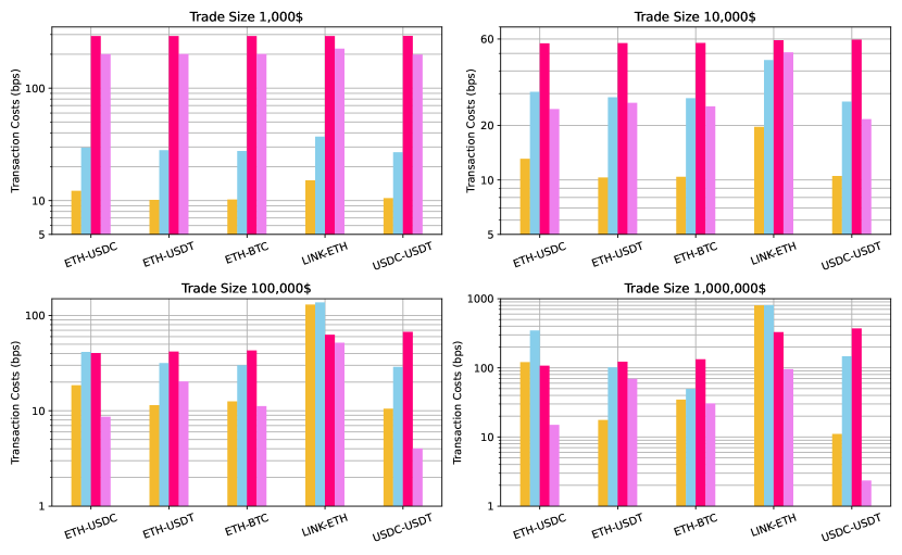
Figure 12: Transaction Costs (Excluding Deposit and Withdrawal Fees). The figure presents average transaction costs, similar to Figure 6. For Uniswap v2 and Uniswap v3, these are computed as in equation (15). For Binance and Kraken, instead, the figures are based on equation (14), but setting the deposit-withdrawal fees $DW_{X,Y}$ to zero. The transaction costs are computed at the hourly frequency for the five pairs in our sample and for different trade sizes ($10^{3},10^{4},10^{5}$, and $10^{6}$ US dollars), then averaged from February 2021 to February 2023. For Uniswap v3, daily and for each trade size, we consider the liquidity pool offering the lowest transaction costs among those available for the specific exchange pair. The vertical axis employs a logarithmic scale and is reported in basis points.

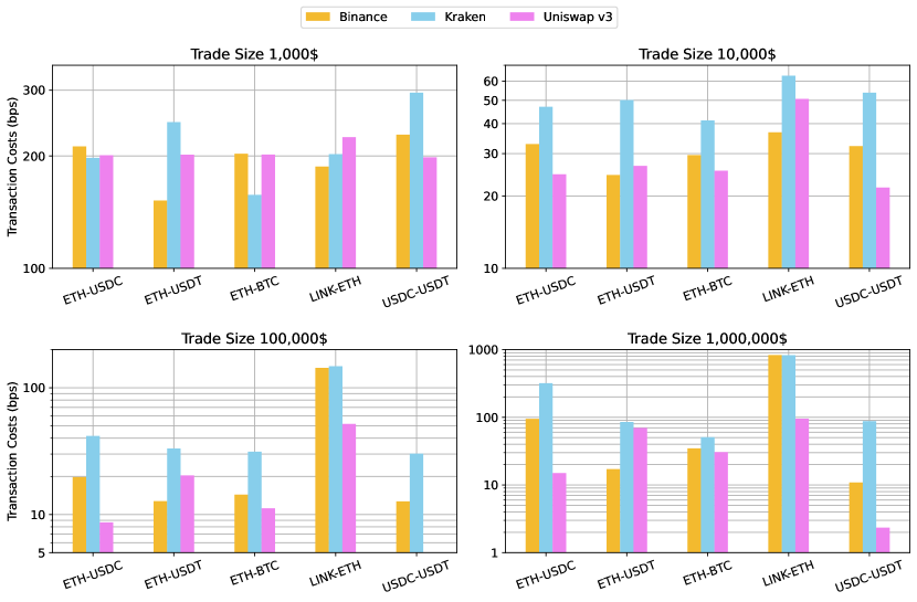
Figure 13: Transaction Costs (Uniswap v3 Period). The figure is similar to 6, but based on the subsample in which Uniswap v3 is present. It presents transaction costs, computed as in equation (14) for the LOB-based Binance and Kraken and on equation (15) for the AMM-based Uniswap v3. The transaction costs are computed at the hourly frequency for the five pairs in our sample and for different trade sizes ($10^{3},10^{4},10^{5}$, and $10^{6}$ US dollars), then averaged from May, 2021 to February, 2023. As discussed in Section V, the displayed transaction costs include B/A spreads, exchange fees, and settlement fees (gas fees for Uniswap v3, and deposit and withdraw fees for the two CEXs). For Uniswap v3, daily and for each trade size, we consider the liquidity pool offering the lowest transaction costs among those available for the specific exchange pair. The vertical axis employs a logarithmic scale and is reported in basis points.

Our analysis is rounded off with two additional investigations to ensure the robustness of our findings. First, to acknowledge the possibility for CEX users to perform multiple trades while keeping their capital in the exchange, we re-run the analysis by removing DW fees for Binance and Kraken. Results, reported in Figure 12 of the Internet Appendix, show that ignoring DW fees significantly reduces CEX TCs associated with smaller trade sizes. For medium and large transactions, instead, removing DW fees has an immaterial effect on TCs. Therefore, for large enough trade sizes, our previously discussed findings remain robust under different assumptions regarding the deposit and withdrawal fees imposed by CEXs, ultimately leading to similar qualitative conclusions. Second, as Uniswap v3 was launched in May 2021, its TCs are averaged over a smaller sample size compared to other DEXs, which could potentially result in an imbalanced comparison. To address this issue, we re-run our analysis on the v3 subsample starting from May 2021. The outcomes of this exercise, detailed in Figure 13 of the Internet Appendix, exhibit no significant discrepancy compared to our previously reported results.

D.   Introduction of Uniswap v3

The previous analysis shows that the introduction of Uniswap v3 coincided with a reduction in DEX transaction costs. To provide more causal evidence of enhanced market quality, we run difference-in-differences regressions concerning transaction costs. The idea is to test whether the introduction of v3 led to a significant decrease in trading costs on DEXs, using the corresponding CEX metrics as the control group. This approach naturally controls for potential confounding factors, contemporaneous to the introduction of v3, that may have caused a global improvement in the quality of cryptocurrency markets.

After ensuring that the Parallel Trend Assumption is met, we consider a window of six months around the deployment of Uniswap v3 (May 5th, 2021), and constructing an hour-pair-level panel of the best transaction costs offered by DEXs and CEXs. Those are constructed by taking the minimum between Uniswap v2 and v3, and Binance and Kraken, respectively. The first result is graphically presented in the top panel of Figure 9, illustrating the temporal progression of the monthly average DEX and CEX transaction costs, averaged across all pairs. This visualization suggests that the launch of v3 operating the DPR and MFT systems has brought DEX transaction costs down to a level that matches those of CEXs, thereby making DEXs highly competitive in this dimension.

We then advance towards a more structured analysis, implementing a difference-in-differences regression of transaction costs at the hour-pair-exchange level. In this configuration, the treatment group comprises each pair quoted on DEXs, while the control group includes the same pairs quoted on CEXs. Table V report results from the exercise, where the dependent variable is regressed on a time dummy ”V3” indicating the period following v3’s deployment, and a treatment dummy ”DEX” indicating decentralized exchanges, and their interaction. The coefficient on the interaction term from specification (1) is negative and highly statistically significant, suggesting that v3 caused a decline in DEX transaction costs. The estimated coefficients also indicate that the effects are economically significant, with a $82\%$ reduction of DEX transaction costs relative to CEXs. Specification (2) shows that these results are robust to the inclusion of weekly and pair fixed effects.

E.   Time Series Properties

In this subsection, we focus on the time-series variation of transaction costs (TCs) of centralized and decentralized exchanges as well as their spread. To guide our analysis, we draw on the hypotheses tested in traditional financial securities and in the discussion formalized above, specific to cryptocurrencies and their exchange systems. First, it is well established that the transaction costs of many financial securities, including equities and FX rates, are persistent. Therefore, we test whether this is true for cryptocurrencies but distinguishing between the persistence of transaction costs in CEXs and DEXs. Second, previous literature has documented a significant commonality in liquidity of stocks (Chordia et al., , 2000) that is even stronger for FX markets (Karnaukh et al., , 2015). Here, we refine these tests for cryptocurrencies. Specifically, we test whether there is liquidity commonality between currency pairs within CEX and DEX exchanges, and across CEXs and DEXs. Third, transaction costs typically increase with the intensity of exchange activity, as documented recently in FX markets (Ranaldo and Santucci de Magistris, , 2022). In our context, this can be captured by the total trading volume for ETH/USD across all markets and the appreciation of ETH against the U.S. Dollar. Finally, we have demonstrated in Section III that the gas price affects transaction costs, especially for DEXs systems.

To test these correlations, we start by constructing a panel of TCs on DEXs and CEXs, sampled at an hourly frequency by trading pair, taking for DEXs the minimum between the TCs on Uniswap v2 and v3, and for CEXs the minimum between those of Binance and Kraken. We then augment the panel with a set of explanatory variables, including the lagged values of TCs, hourly cross-sectional average TCs by exchange category, hourly percentage changes of ETH price relative to USD, total trading volume for ETH/USD across all markets, and the hourly average gas price on Ethereum Mainnet.

Table VI displays results from a number of panel regressions, in which the dependent variables are DEX TCs, CEX TCs, or the difference between DEX and CEX TCs. All regression models are saturated with pair fixed effects. In specifications (1) and (5) TCs are regressed on their first auto-regressive lag. The positive coefficients on the lags and the sizeable $R^{2}$s, above $67\%$, show that both DEX and CEX TCs are fairly persistent relative to what is found in FX markets (Ranaldo and Santucci de Magistris, , 2022). A similar consideration applies to the predictability of TCs.

Specifications (2) and (7) focus on the commonality of TCs across pairs within the same exchange type. In the former, the regressor is the hourly average TCs across CEX exchanges, excluding the target pair, while in the latter the regressor is the hourly average TCs across DEX exchanges, excluding the target pair. The estimated coefficients are highly significantly positive in both cases with $R^{2}$ above $87\%$ for CEX and above $95\%$ for DEX, suggesting a high degree of within-exchange commonality, particularly marked in the case of DEX. Specifications (3) and (6) are aimed at capturing the cross-exchange commonality in liquidity, regressing CEX TCs on the DEX average and, vice-versa, DEX TCs on the CEX average. The estimated positive coefficients and the high coefficients of determination, above $75\%$, indicate the presence of a strong commonality between DEXs and CEXs. Again, the commonality in liquidity of cryptocurrencies appears to be stronger than that documented in FX markets (Karnaukh et al., , 2015) both within the same exchange and across different exchange systems.

Specifications (4) and (8) include a set of regressors related to market conditions, including the total trading volume of the ETH token across CEX and DEX exchanges, in US Dollars; the ETH percentage return versus the US Dollar during the previous 24 hours; and the average gas price for Ethereum transactions recorded in the blocks validated during the same hour. The resulting estimates indicate that TCs of both CEX and DEX are positively correlated to ETH returns and trading volume and, mechanically, are increasing in the Ethereum gas price. In general, these results confirm that transaction costs increase when trading activity is more intense.

Finally, in specification (9), the TC differential between DEX and CEX is linked to the aforementioned market-condition variables, with the resulting coefficients exhibiting positivity and statistical significance. These findings suggest that TCs on DEXs have greater responsiveness to ETH returns and trading volumes. Furthermore, consistent with the previously discussed substantial role of gas fees in DEXs, TCs on DEXs exhibit a stronger sensitivity to fluctuations in the Ethereum gas price.

To gain deeper insight into the impact of gas fees on our findings, we conduct the regressions again, this time excluding gas fees from the TCs calculation. The general picture is confirmed but some differences are noteworthy, as reported in Table VIII of the online appendix. First, we notice an enhanced degree of persistence for both CEXs and DEXs, confirming that changes in gas prices account for a substantial portion of the time-series variation. Moreover, we still find indications of within-exchange-type commonality, albeit diminished. It is intriguing that the decrease in CEX commonality is far more significant, suggesting that gas prices contribute sensitively to common movements of market liquidity in CEXs. Ultimately, the gas price still exhibits a positive and highly significant correlation with DEX TCs but not with CEX TCs, both purged of gas fees. This suggests that the time-series variation in gas price accounts for other underlying factors affecting the quoted spread in DEXs.

VI.   Price Efficiency

Finite liquidity and transaction fees constitute frictions limiting arbitrage forces, allowing deviations from efficient prices to persist and blurring the informativeness of transaction prices. We explore deviations from the law of one price by focusing on triangular arbitrage and relating it to liquidity levels. Performed in only one specific market and nearly risk-free, this arbitrage condition is the ideal laboratory for identifying market-specific frictions and for comparing the price efficiency of different market venues. A triangular arbitrage opportunity arises when the law of one price is violated for a closed triplet of currency pairs $X\leftrightarrow Y$, $Y\leftrightarrow Z$, and $Z\leftrightarrow X$. A direct measure of the deviation from the law of one price is

$$\theta=\,P_{XY}\,P_{YZ}\,P_{ZX}-1\,,$$ (16)

where $P_{AB}$ is the quoted price of $A$ in units of $B$. A triangular trade is profitable only if the magnitude of $\theta$ is sufficiently large or, more precisely, the net expected profits $\theta$ of a triangular trade must be higher than the costs of executing the three associated transactions. Hence, assuming profitable arbitrage opportunities do not arise in equilibrium, the observed distribution of $\mid\theta\mid$ is positively related to transaction costs and, potentially, other frictions impeding arbitrage activity.

We consider five exchange triplets, namely ETH-USDC-USDT, BTC-ETH-USDC, BTC-USDC-USDT, BTC-ETH-USDT, and ETH-LINK-USDT. For each triplet, we sample $\theta$ at an hourly frequency and by exchange, employing distinct definitions for quoted prices, depending on the exchange. For CEXs, we use the mid-price, that is, the average between the best ask and the best bid; For Uniswap v2, we use the ratio between the reserves of the two tokens, as in (1); For Uniswap v3 we retrieve historical quoted prices from Dune.com. We then average the resulting hourly deviations over the sample period from March 2021 to February 2023.

A.   Results on Price Efficiency

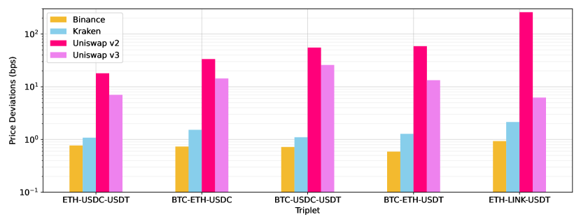
Figure 7: Average Price Deviations. The figure displays price inefficiency levels, proxied by the absolute value of price deviations from the law of one price, defined by equation (16). These are computed separately for each trading triplet and for each exchange, namely for CEXs Binance and Kraken, and for DEXs Uniswap v2 and Uniswap v3. Absolute price deviations are first estimated at the hourly frequency for the five triplets in our sample, then averaged from March 2021 to February 2023. For Uniswap v3 the estimation is based on a shorter sample starting on May 5th, 2021, when the exchange was launched. For the pairs involving USDC in Binance, the estimation is based on a truncated sample that ends on September 29th, 2022, when the exchange ceased quoting trading pairs in USDC. The vertical axis employs a logarithmic scale and is reported in basis points.

Figure 7 presents the results, displaying the average log levels of price deviations. It is evident that DEXs are far less price-efficient than their centralized counterparts. For most triplets, Uniswap v2 price deviations average between $10$ and $60$ bps, while they rise above $200$ bps for the less liquid ETH-LINK-USDT. Uniswap v3 performs significantly better than its predecessor, with average deviations ranging between $6$ and $30$ bps. These estimates are significantly higher than those for CEXs, which are below $3$ bps for all triplets. Binance dominates regarding price efficiency, with average deviations below $1$ basis point.

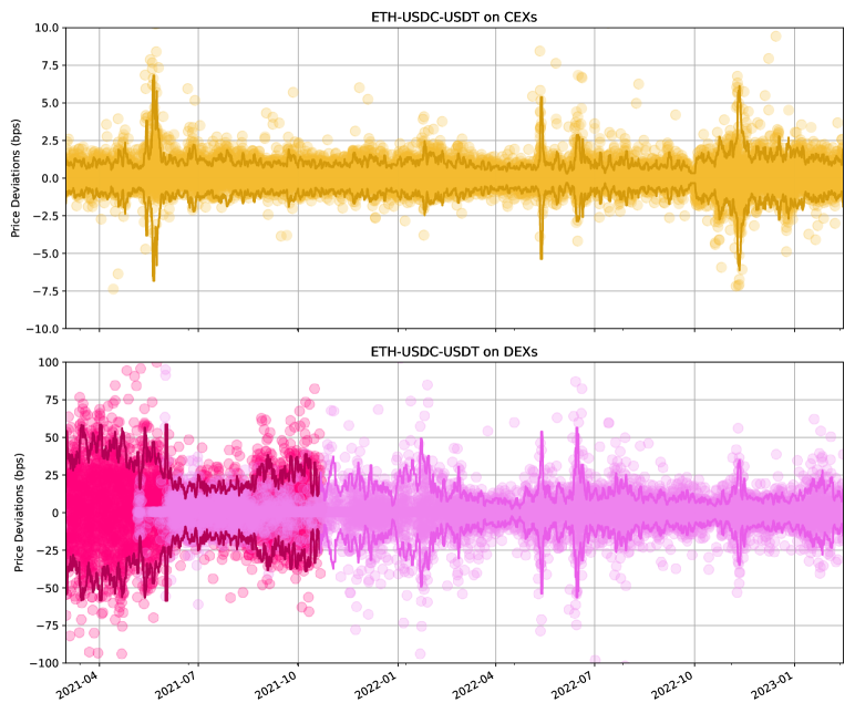
Figure 8: Price Deviations. The figure displays the estimated price deviations from the law of one price $\theta$ for the triplet USDC-USDT-ETH, at an hourly frequency over the period from March 2021 to February 2023. The top panel illustrates deviations for CEXs. The time series is derived by selecting the minimum deviation (in absolute value) between Binance and Kraken for each hour. The bottom panel displays the deviations for DEXs. This time series is generated by selecting the smallest absolute deviation between Uniswap v2 and Uniswap v3 at each hourly interval. If the minimum deviation is found in v2, the corresponding data point is marked in pink, whereas if v3 has the minimum deviation, the data point is highlighted in violet. Please note that the vertical axes of the two panels have different scales. On both panels, the solid lines represent the top decile of the distribution of absolute deviations, estimated on a 7-day rolling window.

Figure 8 displays the time-series evolution of hourly price deviations for the ETH-USDC-USDT triplet, with each dot representing an observation. The top panel presents the series for CEXs, defined as the price deviation with the minimum absolute value, on each hour, between those of Binance and Kraken. Similarly, the bottom panel plots the hourly price deviation with the minimum absolute value among those recorded on Uniswap v2 and Uniswap v3. To visualize the introduction of v3 in May 2021, dots on this panel are colored in pink when the minimum is achieved in v2, and in violet when the minimum is achieved in v3. On both panels, the solid lines represent the top decile of the distribution of absolute deviations, estimated on a 7-day rolling window. The main takeaway of the figure is that the dominance of DEXs regarding price efficiency is stable across the sample period, with deviations an order of magnitude smaller than in DEXs. It also shows, however, that the introduction of Uniswap v3 is followed by a significant improvement in DEX price efficiency, decreasing by more than 50% from the beginning of the sample.

We argue that the under-performance of DEXs in terms of price efficiency is not surprising, as it can be explained by the absence of delegated custody. To see this, note that CEX arbitrageurs are likely to have their capital readily available in the exchange. The reason is that moving capital from a non-custodial wallet to a CEX is costly and takes a significant amount of time. Given a competitive environment, arbitrageurs are thus incentivized to delegate the custody of their arbitrage capital to the exchange at the expense of counterparty risk exposure. Consequently, their transactions are not subject to deposit and withdrawal fees which, as we saw in Section V, constitute a sizeable cost. Moreover, since gas-related costs are independent of trade size, avoiding those allows arbitrageurs to transact any amount of capital – even of very small dollar amounts – whenever an arbitrage opportunity is available.

DEX arbitrageurs, on the contrary, do not have the option to deposit their arbitrage capital in the exchange to avoid gas costs. As a first-order consequence, they are forced to cover the gas cost of each transaction, thus making their arbitrage trades more costly. Further, a second-order implication is that, as is the case with models that have entry costs, arbitrageurs face a trade-off between the gas costs and price impact. The former is reduced (in $\%$) by increasing $\Delta x$, while the latter increases with $\Delta x$. Therefore, DEX arbitrageurs do not profit from trading small dollar amounts and only act when the available liquidity allows for larger enough transactions.

Another factor that may contribute to the superior price efficiency of CEXs, is related to the effective exchange fees. While on DEXs fees apply to all market participants, CEXs can offer lower fees to arbitrageurs generating large trading volume. Further, a CEX may perform arbitrage activity itself, avoiding exchange fees altogether. As triangular arbitrages require three transactions, the exchange fees add up to a significant determinant of the net profitability of the trade.

All in all, these institutional differences between CEXs and DEXs, together with relatively high gas prices, play an important role in explaining the significant difference in price efficiency between the two categories of exchanges. Although advancements in blockchain technology will likely result in lower gas prices in the future, the current architecture of DEXs, centered around AMM, makes it challenging to achieve price efficiency levels comparable to that of CEXs.

To conclude this section, we note that, while CEXs enjoy higher levels of price efficiency, they may not offer the best experience from an operational point of view. In fact, taking the perspective of a CEX user keeping her funds in a non-custodial wallet, the significant time delay affecting deposits induces a trade-off between price efficiency and speed of execution. Conversely, even if DEX quoted prices are further away from their efficient levels, the user can settle a transaction with a significantly shorter time delay.

B.   Introduction of Uniswap v3

As we have already done above by studying market liquidity, we perform a difference-in-differences regression to assess whether the introduction of Uniswap v3 led to an improvement in market quality. This time, however, we take advantage of this quasi-natural laboratory to observe a causal effect on our measure of price efficiency.

Similarly to the previous setting, this approach uses the corresponding CEX metrics as the control group and it naturally controls for potential confounding, common factors.. We construct an hour-triplet-level panel with the minimum absolute deviations by exchange category.

A preliminary result is provided graphically in the bottom panel of Figure 9, which displays the time series of the average monthly price deviations, averaged across pairs. This suggests that, while the price efficiency gains from v3 are substantial, they are not sufficient to eliminate the gap with CEXs. Table V report results from the difference-in-differences, where the dependent variable measuring price errors is regressed on a time dummy ”V3” indicating the period following v3’s deployment, and a treatment dummy ”DEX” indicating decentralized exchanges, and their interaction. The coefficient on the interaction term from specifications (2) is negative and highly statistically significant, suggesting that v3 caused a decline in price deviations. The estimated coefficients indicate that the effects are economically significant, with a $48\%$ reduction in DEX price deviations relative to CEXs. Specification (4) shows that these results are robust to the inclusion of weekly and triplet fixed effects.

All in all, this analysis provides evidence of an increase in price efficiency fostered by the implementation of the DPR and MFT systems, making it possible for LPs to take leverage on their liquidity positions and to choose the level of exchange fees. However, this improvement is still not enough to surmount the bar of market quality set by CEX systems.

VII.   Conclusion

We describe the institutional nuances of decentralized exchanges (DEXs) utilizing Automated Market Making (AMM), contrasting these with centralized exchanges (CEXs) employing limit order books (LOBs). Furthermore, we discuss the AMM price formation mechanism, regulated by an algorithm that autonomously sets transaction prices based on the liquidity contributed by market participants; the concept of self-custody, and the risks faced by CEX users when depositing crypto-assets into a centralized exchange; and the array of advantages DEXs offer in terms of accessibility, security, resistance to censorship, and settlement.

Central to our study is an examination of two vital facets of market quality: (i) market liquidity, whereby we measure all cost components associated with trading on CEXs and DEXs, and (ii) price efficiency, through an analysis of deviations from the triangular no-arbitrage condition. The ensuing image portrays a DEX landscape that is competitive in terms of transaction costs, particularly in the wake of the introduction of Uniswap v3. Conversely, CEXs enjoy higher levels of price efficiency by adhering more closely to the law of one price. In this context, we identify elevated gas prices and exchange fees as the main frictions harming DEX price efficiency. This is especially pertinent to triangular price deviations, which necessitate the execution of three separate transactions.

Subsequently, we offer causal evidence that Uniswap v3, the most recent DEX upgrade, has significantly enhanced DEX market quality. We propose that this beneficial impact is spurred by two novel mechanisms, namely, the Discretionary Price Range (DPR) and Multiple Fee Tiering (MFT) systems. The former enables liquidity providers (LPs) to employ leverage by concentrating their liquidity within a custom price range, resulting in narrower spreads for less-volatile exchange pairs, in particular for stablecoin pairs. The latter introduces multiple pools for each exchange pair, with distinct fee levels, providing traders the option to choose the most convenient venue.

Given these insights, we assert that the innovative market structure of decentralized crypto exchanges holds promise, though it has yet to fully realize its potential. Our analysis suggests that substantial enhancements could stem from a reduction in gas prices facilitated by advancements in blockchain technology, and from prospective upgrades to the AMM system in the future. We posit that the AMM system may be applied to other asset classes in the near future. It could then rival existing LOB-based exchanges in terms of market quality, thereby answering the Glosten, (1994)’s long-standing question that the electronic LOB system is not inevitable after all.

Tables and Figures

	N	Mean	Std	1%	10%	50%	90%	99%
Panel A: Uniswap v2 Exchange Pairs
Liquidity (Million USD)	5	33.79	31.35	1.69	9.97	23.85	60.86	72.55
Volume (Million USD)	5	16.62	16.43	1.84	3.85	8.57	34.00	34.83
Swaps (Thousands)	5	1.57	1.67	0.36	0.36	0.38	2.99	3.75
Panel B: Uniswap v3 Exchange Pairs
Liquidity (Million USD)	5	180.29	160.38	18.52	71.99	106.39	338.49	366.04
Volume (Million USD)	5	125.75	165.74	5.15	57.71	64.75	83.52	417.64
Swaps (Thousands)	5	1.74	1.96	0.16	0.59	0.69	2.33	4.92
Panel C: Gas Prices
Gas Price (GWEI)	17,497	68.473	99.755	8.447	15.433	44.848	148.192	287.456
Cost of a Swap (USD)	17,497	20.466	34.367	1.013	2.048	10.817	50.585	100.510

Table I: Summary Statistics. The first two panels display statistics on the 5 exchange pairs analyzed in our study, reporting the total value of deposited liquidity (in million USD), the total traded volume (in million USD), and the total number of swap transactions (in thousands). Panel A focuses on Uniswap v2, with figures based on data from March 2021 to February 2022. Panel B focuses on Uniswap v3, with figures based on data from June 2021 to February 2023. In Uniswap v3 the MFT system, described in Section B.2, allows for multiple liquidity pools per exchange pair. We thus aggregate at the pair level by taking the sum of liquidity, volume, and swaps across sibling pools. Panel C reports statistics for gas prices on the Ethereum blockchain over the period from March 2021 to February 2023 at the hourly frequency.

Pair	Binance	Kraken	Uniswap v2	Uniswap v3
ETH-USDT	1,578.891	84.572	56.429	122.113
ETH-BTC	302.811	16.052	8.877	97.319
USDC-USDT	188.407	10.733	3.427	86.131
ETH-USDC	57.720	3.410	58.584	212.024
LINK-ETH	5.281	0.297	5.290	7.287
Fraction of Total Volume	13.828%	18.453%	29.901%	33.186%

Table II: Trading Volume by Pair. The table reports the daily average trading volume, denoted in millions of USD, for the five trading pairs considered in our empirical analysis. To select these pairs, we start by considering the intersection of trading pairs available in Binance, and Kraken, Uniswap v2, and Uniswap v3. We then compute percentile rankings of average daily volumes in USD for each of the three exchanges available at the beginning of our sample, take their average, and select the first five pairs ranked by the resulting metric. The fraction of the total volume represented by the five trading pairs combined is reported below. The estimates are based on data from March 2021 to February 2023 for Binance and Kraken, on data from March 2021 to February 2022 for Uniswap v2, and on data from June 2021 to February 2023 for Uniswap v3.

Pair		ETH-USDC	ETH-USDT	ETH-BTC	LINK-ETH	USDC-USDT
Panel A: Uniswap v2
Exchange Fees		30.000	30.000	30.000	30.000	30.000
B/A Spread	1,000	0.077	0.093	0.103	0.303	0.347
	10,000	0.774	0.925	1.032	3.030	3.466
	100,000	7.739	9.249	10.313	30.252	34.594
	1,000,000	77.115	92.090	102.597	298.139	340.027
Gas Fees	1,000	260.717	260.717	260.717	260.689	260.717
	10,000	26.072	26.072	26.072	26.069	26.072
	100,000	2.607	2.607	2.607	2.607	2.607
	1,000,000	0.261	0.261	0.261	0.261	0.261
Total TCs	1,000	290.795	290.810	290.820	290.992	291.064
	10,000	56.846	56.997	57.104	59.099	59.537
	100,000	40.347	41.856	42.920	62.859	67.201
	1,000,000	107.376	122.350	132.858	328.400	370.288
Panel B: Uniswap v3
Exchange Fees		Variable	Variable	Variable	Variable	Variable
B/A Spread	1,000	0.270	0.219	0.112	2.817	0.002
	10,000	0.457	1.816	0.474	2.689	0.007
	100,000	1.738	9.567	3.540	22.170	0.028
	1,000,000	10.672	53.996	16.553	86.390	0.124
Gas Fees	1,000	196.299	196.299	196.299	196.299	196.299
	10,000	19.630	19.630	19.630	19.630	19.630
	100,000	1.963	1.963	1.963	1.963	1.963
	1,000,000	0.196	0.196	0.196	0.196	0.196
Total TCs	1,000	200.763	201.518	201.591	224.431	198.329
	10,000	24.616	26.657	25.481	50.659	21.667
	100,000	8.676	20.354	11.196	51.808	4.025
	1,000,000	14.994	69.437	30.527	95.404	2.346

Table III: Transaction Costs – Breakdown by Trade Size. The table displays the average transaction costs for each exchange pair in our sample, for different trade sizes denominated in USD, for Uniswap v2, Uniswap v3, Binance, and Kraken. The figures are based on equation (15) for DEX and equation (14) for CEXs and are expressed in basis points. They are first computed at the hourly frequency and then averaged from March 2021 to February 2023. For each pair, we present a breakdown of total transaction costs by their individual components: exchange fees, B/A spread, and gas fees or deposit-withdrawal fees. For Uniswap v3, daily and for each trade size, we consider the liquidity pool offering the lowest transaction costs among those available for the specific exchange pair.

Pair		ETH-USDC	ETH-USDT	ETH-BTC	LINK-ETH	USDC-USDT
Panel C: Binance
Exchange Fees		10.000	10.000	10.000	10.000	10.000
B/A Spread	1,000	0.230	2.201	0.137	5.137	0.501
	10,000	0.404	3.089	0.319	9.654	0.504
	100,000	2.552	8.519	1.437	120.037	0.526
	1,000,000	24.644	111.019	7.621	790.367	1.059
DW Fees	1,000	192.263	203.699	148.538	174.739	225.417
	10,000	19.226	20.370	14.854	17.474	22.542
	100,000	1.923	2.037	1.485	1.747	2.254
	1,000,000	0.192	0.204	0.149	0.175	0.225
Total TCs	1,000	202.494	215.900	158.676	189.876	235.918
	10,000	29.630	33.459	25.172	37.128	33.046
	100,000	14.475	20.556	12.922	131.785	12.780
	1,000,000	34.836	121.222	17.770	800.542	11.284
Panel D: Kraken
Exchange Fees		26.000	26.000	26.000	26.000	26.000
B/A Spread	1,000	1.611	3.537	2.008	11.002	0.860
	10,000	2.253	4.639	2.622	19.954	1.092
	100,000	4.028	15.360	5.689	111.066	2.859
	1,000,000	23.713	321.179	75.670	781.425	121.095
DW Fees	1,000	137.640	172.690	222.693	165.577	278.939
	10,000	13.764	17.269	22.269	16.558	27.894
	100,000	1.376	1.727	2.227	1.656	2.789
	1,000,000	0.138	0.173	0.223	0.166	0.279
Total TCs	1,000	165.250	202.226	250.701	202.579	305.799
	10,000	42.017	47.908	50.891	62.512	54.986
	100,000	31.405	43.087	33.916	138.722	31.648
	1,000,000	49.851	347.352	101.892	807.590	147.374

Pair		ETH-USDC	ETH-USDT	ETH-BTC	LINK-ETH	USDC-USDT
Panel A: Uniswap v2
Exchange Fees		30.000	30.000	30.000	30.000	30.000
B/A Spread	Mean	0.774	0.925	1.032	3.030	3.466
	Std	0.159	0.207	0.376	0.970	1.326
Gas Fees	Mean	26.072	26.072	26.072	26.069	26.072
	Std	22.906	22.906	22.906	22.906	22.906
Total TC	Mean	56.846	56.997	57.104	59.099	59.537
	Std	22.897	22.895	22.772	22.477	22.862
Panel B: Uniswap v3
Exchange Fees		4.529	5.211	5.378	28.341	2.030
B/A Spread	Mean	0.457	1.816	0.474	2.689	0.007
	Std	0.862	2.751	1.237	3.189	0.105
Gas Fees	Mean	19.630	19.630	19.630	19.630	19.630
	Std	37.529	37.529	37.529	37.529	37.529
Total TC	Mean	24.616	26.657	25.481	50.659	21.667
	Std	37.616	37.224	37.504	38.308	37.884
Panel C: Binance
Exchange Fees		10.000	10.000	10.000	10.000	10.000
B/A Spread	Mean	3.089	0.319	0.404	9.654	0.504
	Std	1.994	0.461	0.576	4.033	0.132
DW Fees	Mean	20.370	14.854	19.226	17.474	22.542
	Std	15.910	15.269	18.331	16.349	21.801
Total TC	Mean	33.459	25.172	29.630	37.128	33.046
	Std	16.308	15.333	18.376	15.605	21.807
Panel D: Kraken
Exchange Fees		26.000	26.000	26.000	26.000	26.000
B/A Spread	Mean	4.639	2.622	2.253	19.954	1.092
	Std	5.084	2.610	1.631	15.618	1.104
DW Fees	Mean	17.269	22.269	13.764	16.558	27.894
	Std	14.352	14.352	15.035	16.180	20.282
Total TC	Mean	47.908	50.891	42.017	62.512	54.986
	Std	15.156	14.579	14.784	19.356	20.352

Table IV: Transaction Costs – Breakdown by Component. The table displays the time-series distribution of transaction costs for each exchange pair in our sample, for Uniswap v2, Uniswap v3, Binance, and Kraken, expressed in basis points. The figures are based on equation (15) for DEX and equation (14) for CEXs. They are computed at the hourly frequency from March 2021 to February 2023, assuming a transaction size of $10,000\$$. For each pair, we present a breakdown of total transaction costs by their individual components: exchange fees, B/A spread, and gas fees or deposit-withdrawal fees. For Uniswap v3, each day we consider the liquidity pool with the lowest transaction costs among those available for the specific exchange pair.

	(1)	(2)	(3)	(4)
Dep. Variable	Transaction	Transaction	Price	Price
	Costs	Costs	Deviations	Deviations
$\text{DEX}\times\text{V3}\qquad$	-25.941***	-25.941***	-14.251***	-13.753***
	(-4.673)	(-4.671)	(-4.947)	(-4.722)
DEX	31.677***	31.677***	28.919***	29.033***
	(16.961)	(16.956)	(7.629)	(7.711)
V3	-4.270*		-0.909**
	(-1.899)		(-2.002)
Intercept	32.936***		1.648***
	(18.741)		(3.757)
Observations	45,042	45,042	42,971	42,971
R-squared	0.313	0.595	0.067	0.092
Week FEs		Yes		Yes
Pair/Triplet FEs		Yes		Yes

Table V: Introduction of Uniswap v3. The table reports results from a difference-in-differences regression around the introduction of Uniswap v3, deployed on the Ethereum Mainnet on May 5th, 2021. In specifications (1) and (2) the dependent variable is the hourly average transaction costs, as defined in (14) and (15), and the regression model is estimated on a panel at the exchange-pair-hour level, meaning that we include hourly observations for the 5 pairs in our sample, separately for each exchange. In specifications (3) and (4) the dependent variable is the hourly average price deviations from the law of one price, as defined in (16), and the regression model is estimated on a panel at the exchange-triplet-hour level, meaning that we include hourly observations for the 5 triplets in our sample, separately for each exchange. The treatment dummy ”DEX” is equal to $1$ for pairs and triplets on Uniswap v2 and v3, while it equals zero for Binance and Kraken. The post dummy ”V3” equals zero before the introduction of Uniswap v3, and one afterwards. We saturate the regression model with triplet and week fixed effects. T-stats are reported in parentheses and are based on standard errors double-clustered by week and pair or by week and triplet. Asterisks denote significance levels (***$=1\%$, **$=5\%$, *$=10\%$).

	(1)	(2)	(3)	(4)	(5)	(6)	(7)	(8)	(9)
Dep. Variable	CEX	CEX	CEX	CEX	DEX	DEX	DEX	DEX	DEX - CEX
Lagged CEX TC	0.810***
	(15.128)
Lagged DEX TC					0.808***
					(8.185)
Average CEX TCs		1.015***				2.287***
		(21.249)				(21.670)
Average DEX TCs			0.376***				1.001***
			(22.065)				(95.879)
ETH Volume in USD				0.068				0.608***	0.472***
				(1.123)				(5.100)	(3.167)
ETH Return				5.892***				26.668***	13.233***
				(2.909)				(7.060)	(4.021)
Gas Price				0.144***				0.360***	0.007
				(19.006)				(37.172)	(0.835)
Observations	85,485	85,485	85,485	85,485	85,485	85,485	85,485	85,485	85,485
R-squared	0.675	0.873	0.754	0.754	0.671	0.836	0.958	0.889	0.748
Pair FEs	Yes	Yes	Yes	Yes	Yes	Yes	Yes	Yes	Yes

Table VI: Transaction Costs – Time Series. The table presents the findings of panel regression analyses on transaction costs, sampled at an hourly frequency by trading pair, and their relationship with various explanatory factors. The first four specifications focus on the transaction costs (TC) of CEXs, as outlined in equation (14). The dependent variable is determined by selecting the minimum value between Binance and Kraken at the pair-hour level. The subsequent four specifications concentrate on the transaction costs of DEXs, as defined in equation (15), with the dependent variable derived from the minimum value between Uniswap v2 and Uniswap v3 at the pair-hour level. The final specification’s dependent variable is the difference in transaction costs between DEXs and CEXs at the pair-hour level. In specifications (1) and (5) the dependent variable is regressed on its first auto-regressive lag. In specification (2) the regressor is the hourly average transaction costs across CEX exchanges, excluding the target pair. Similarly, in specification (7) the regressor is the hourly average transaction costs across DEX exchanges, excluding the target pair. In specification (3) and (6) we regress CEX transaction costs on the DEX average and, vice-versa, DEX transaction costs on the CEX average. Specifications (4) and (8) include a set of regressors related to market conditions, including (i) the total trading volume of the ETH token across CEX and DEX exchanges, in US Dollars; (ii) the ETH percentage return versus the US Dollar during the previous 24 hours; and (iii) the average gas price for Ethereum transactions recorded in the blocks validated during the same hour. Finally, in specification (9) the difference between DEX and CEX transaction costs is regressed onto the aforementioned set of market condition-related regressors. The regression models are saturated with pair fixed effects. T-stats are reported in parentheses and are based on standard errors double-clustered by week and pair. Asterisks denote significance levels (***$=1\%$, **$=5\%$, *$=10\%$).

	(1)	(2)	(3)	(4)
Dep. Variable	Volume	Volume	log(Volume)	log(Volume)
DEX $\times$ FTX	5.550***	5.550***	0.308***	0.308***
	(5.951)	(6.753)	(3.908)	(4.714)
DEX	-14.720***	-14.720***	-1.788***	-1.788***
	(-20.182)	(-23.127)	(-32.957)	(-38.418)
FTX	-5.779***	-6.282***	-0.405***	-0.416***
	(-6.267)	(-5.059)	(-6.434)	(-5.176)
Intercept	16.587***		2.814***
	(22.919)		(63.114)
Observations	236	236	236	236
R-squared	0.760	0.816	0.884	0.922
Month FE		Yes		Yes

Table VII: FTX Event Study. The table presents findings from difference-in-differences regression analyses of the trading activity on CEX and DEX exchanges around the collapse of the FTX exchange on November 10th, 2022. The sample encompasses a period of two months before and after the event, ranging from September 9th, 2022 to January 9th, 2023. The dependent variable, that is the trading volume sampled at the daily frequency broken down by CEXs (Binance and Kraken) and DEXs (Uniswap v2 and v3), is regressed on a treatment dummy (DEX) indicating DEXs, a time dummy (FTX) indicating the period after the FTX collapse, and their interaction. In the first two specifications the trading volume is expressed in billion US Dollars, while the next two specifications employ the logarithm of the trading volume as the dependent variable. In specifications (2) and (4) we saturate the regression model with month fixed effects. T-stats are reported in parentheses and are based on robust standard errors. Asterisks denote significance levels (***$=1\%$, **$=5\%$, *$=10\%$).

Figure 5: Distribution of DEX Trade Sizes. The figure presents the frequency distribution of trade sizes in US Dollars for swap transactions executed on Uniswap v2 ad Uniswap v3, during our sample period (from March 2021 to February 2023) and restricting to the five pairs featured in our study, namely ETH-USDC, ETH-USDT, ETH-BTC, LINK-ETH, and USDC-USDT. Swap transactions with a Dollar value below $1$ are excluded, and gas costs are not included. The data is retrieved using a custom query in Dune Analytics based on the ‘uniswap_v2_ethereum.trades’ and ‘uniswap_v3_ethereum.trades’ tables.

Figure 9: Introduction of Uniswap v3. The figures present two event studies around the deployment of Uniswap v3 on the Ethereum MainNet, on May 5th, 2021. In the top panel, we plot the average transaction cost across the five pairs in our sample, on a monthly basis, separately for DEXs and CEXs. The transaction cost measures are defined in (14) and (15). To construct the two time series, for each pair-hour, we select the lowest transaction costs among Uniswap v2 and Uniswap 3 (for DEXs), and among Binance and Kraken (for CEXs). We then take, for each month, the equally weighted average of these values across the five pairs. Similarly, in the bottom panel, we plot the average price deviation across the five triplets in our sample, on a monthly basis, separately for DEXs and CEXs. The price deviation measure is defined in (16). To construct the two time series, for each triplet-hour, we select the lowest transaction costs among Uniswap v2 and Uniswap 3 (for DEXs) and among Binance and Kraken (for CEXs). We then take, for each month, the equally weighted average of these values across the five triplets.

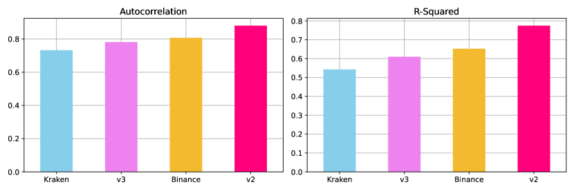
Figure 10: Predictability of Transaction Costs. The figure presents the degree of predictability of transaction costs on different exchanges. For each exchange-pair couple, considering hourly transaction costs for a 10,000$ transaction, we compute the auto-correlation coefficient $\rho$ and run the time series regressions $\text{TC}(t)=\alpha+\beta\;\text{TC}(t-1)+\varepsilon(t)$. We then plot the average auto-correlation coefficient $\rho$ (left panel) and the average $R^{2}$ from the time-series regressions (right panel).

Internet Appendix

A.   A Model of Liquidity Provision

We model a marginal LP in Uniswap v2, who faces the problem of providing the optimal quantity of liquidity to the exchange pair $X/Y$. We assume that the LP is risk-neutral and that the market is perfectly competitive as in, e.g., Glosten and Milgrom, (1985). At time $t=0$ the total liquidity in the pools is equal to $x$, and the LP can add or remove a quantity $\xi$ of liquidity. At time $t>0$, users start to trade on the pair until the trading stops at $t=1$. Let the random variables $V$ denote the total traded volume (in units of $X$) and let $\Delta P=P_{1}/P_{0}$ denote the gross percentage change in the quoted price, respectively, between $t=0$ and $t=1$. As discussed in Section III, the profits and losses of the LP depend on two factors: the fees arising from liquidity takers’ trading volume and the impermanent loss due to changes in quoted prices.

Let $\operatorname{E}[V]$ denote the expected unsigned trading volume and let $\operatorname{E}[IL]$ denote the expected $IL$, both estimated at time $t=0$. The expected fees paid by liquidity takers amount to the product of the exchange fees $f$ and the expected volume $\operatorname{E}[V]$, expressed in units of $X$. Since this amount is distributed by the protocol to the participating LPs on a pro-rata basis, the marginal liquidity provider depositing $\xi$ units of additional liquidity gains in expectation $\frac{\xi}{x+\xi}f\operatorname{E}[V]$ units of $X$, corresponding to a percentage profit of $\frac{f\operatorname{E}[V]}{x+\xi}$. Hence, accounting for both fees and the expected impermanent loss, the net expected percentage profit $\operatorname{E}[R]$ from providing an additional amount $\xi$ of liquidity is equal to

$$\operatorname{E}[R]=\frac{f}{x+\xi}\operatorname{E}[V]-\operatorname{E}[IL]\,.$$

The assumption of perfect competition results in zero expected profits for the LP, hence the equilibrium level of total liquidity $x^{*}=\xi+x$ is given by

$$x^{*}=\frac{f\operatorname{E}[V]}{\operatorname{E}[IL]}$$ (17)

showing that total liquidity increases with the expected trading volume and (percentage) exchange fees remunerating the LP, while it decreases with the expected IL. The equilibrium condition (17) has a clear economic interpretation that is conceptually related to standard microstructure models featuring market makers. First, the level of liquidity $x^{*}$ provided by LPs determines the quoted spread available to traders, as in (3). Second, as noted above, the expected IL can be thought of as a proxy for the level of adverse selection risk faced by LPs. Thus (17) says that spreads are increasing in the level of adverse selection; in other words, LPs require compensation for the losses caused by informed trading.

We use daily liquidity data to test the predictions of our model, proxying for $\operatorname{E}[V]$ with the rolling average of daily traded volume and for $\operatorname{E}[IL]$ with the rolling average of the daily IL, estimated over the previous two weeks. We regress daily log values of empirically observed liquidity on the ones predicted by (17), for $100$ exchange pairs from February 2021 to February 2023. Results are reported in Table IX and Figure 11, showing a highly significant positive correlation between predicted and observed liquidity levels, with a remarkable $R^{2}$ coefficient equal to or higher than $92\%$. The results are robust to the inclusion of pair- and time-fixed effects. Our results are also robust to changing the size of the rolling windows used to estimate $\operatorname{E}[IL]$ and $\operatorname{E}[V]$. In particular we use 5 days and 20 days, corresponding to the median and average duration of liquidity positions reported in O’Neill, (2022), and we find that the resulting R-squared for the baseline specification is 91.38% and 92.50%, respectively. We thus conclude that our partial equilibrium model is empirically relevant, as it is able to capture the main economic trade-off faced by LPs in AMM-based DEXs. At the same time, our findings suggest that LPs behave rationally in the aggregate.

B.   Tables and Figures

	(1)	(2)	(3)	(4)	(5)	(6)	(7)	(8)	(9)
Dep. Variable	CEX	CEX	CEX	CEX	DEX	DEX	DEX	DEX	DEX - CEX
Lagged CEX TC	0.954***
	(30.659)
Lagged DEX TC					0.998***
					(1372.515)
Average CEX TCs		0.803*				-0.585***
		(1.931)				(-3.509)
Average DEX TCs			-0.158***				1.037***
			(-3.127)				(5.451)
ETH Volume in USD				-0.023				0.449***	0.540***
				(-0.348)				(4.258)	(3.507)
ETH Return				-1.586				11.647***	20.776***
				(-0.854)				(3.806)	(6.065)
Gas Price				0.004				0.011***	0.216***
				(0.693)				(2.625)	(18.797)
Observations	85,485	85,485	85,485	85,485	85,485	85,485	85,485	85,485	85,485
R-squared	0.933	0.381	0.272	0.257	0.998	0.568	0.873	0.586	0.315
Pair FEs	Yes	Yes	Yes	Yes	Yes	Yes	Yes	Yes	Yes

Table VIII: Transaction Costs – Time Series (Excluding Gas Costs). The table presents the findings of panel regression analyses on transaction costs, sampled at an hourly frequency by trading pair, and their relationship with various explanatory factors. These regressions are similr to those displayed in VI, with the difference that the transaction costs used as dependent variables do not include gas-related costs (gas fees for DEXs, and DW fees for CEXs). The first four specifications focus on the transaction costs (TC) of CEXs, as outlined in equation (14). The dependent variable is determined by selecting the minimum value between Binance and Kraken at the pair-hour level. The subsequent four specifications concentrate on the transaction costs of DEXs, as defined in equation (15), with the dependent variable derived from the minimum value between Uniswap v2 and Uniswap v3 at the pair-hour level. The final specification’s dependent variable is the difference in transaction costs between DEXs and CEXs at the pair-hour level. In specifications (1) and (5) the dependent variable is regressed on its first auto-regressive lag. In specification (2) the regressor is the hourly average transaction costs across CEX exchanges, excluding the target pair. Similarly, in specification (7) the regressor is the hourly average transaction costs across DEX exchanges, excluding the target pair. In specification (3) and (6) we regress CEX transaction costs on the DEX average and, vice-versa, DEX transaction costs on the CEX average. Specifications (4) and (8) include a set of regressors related to market conditions, including (i) the total trading volume of the ETH token across CEX and DEX exchanges, in US Dollars; (ii) the ETH percentage return versus the US Dollar during the previous 24 hours; and (iii) the average gas price for Ethereum transactions recorded in the blocks validated during the same hour. Finally, in specification (9) the difference between DEX and CEX transaction costs is regressed onto the aforementioned set of market condition-related regressors. The regression models are saturated with pair fixed effects. T-stats are reported in parentheses and are based on standard errors double-clustered by week and pair. Asterisks denote significance levels (***$=1\%$, **$=5\%$, *$=10\%$).

	(1)	(2)	(3)	(4)
Dependent Variable	Log(Liquidity)	Log(Liquidity)	Log(Liquidity)	Log(Liquidity)
Log(Predicted Liquidity)	0.89***	0.61***	0.89***	0.53***
	(29.94)	(12.39)	(30.14)	(10.24)
Constant	5.92***
	(21.71)
Observations	42,293	42,293	42,293	42,293
R-squared	0.92	0.97	0.92	0.98
Pair Fixed Effects	-	Yes	-	Yes
Date Fixed Effects	-	-	Yes	Yes

Table IX: Model Fit. The table reports results from a panel regression of log-observed liquidity levels onto log liquidity levels predicted by the equilibrium model outlined in Section A and computed as in equation (17). Both the dependent and independent variables are computed at the pair-day level for $100$ exchange pairs from February 2021 to February 2022. We saturate the regression model with day- and pair fixed effects. T-stats are reported in parentheses, based on robust standard errors double-clustered at the pair- and day-level. Asterisks denote significance levels (***$=1\%$, **$=5\%$, *$=10\%$).

Figure 11: Model Fit. The figure presents a scatter plot of The observed levels of liquidity (y-axis) and those predicted by our model and computed as in equation (17) (x-axis), based on $42,299$ daily observations of $100$ exchange pairs quoted in Uniswap v2. from February 2021 to February 2022.

References

- Adams et al., (2020) Adams, H., Zinsmeister, N., and Robinson, D. (2020). Uniswap v2 core.
- Adams et al., (2021) Adams, H., Zinsmeister, N., Salem, M., Keefer, R., and Robinson, D. (2021). Uniswap v3 core.
- Aigner and Dhaliwal, (2021) Aigner, A. A. and Dhaliwal, G. (2021). Uniswap: Impermanent loss and risk profile of a liquidity provider. arXiv preprint arXiv:2106.14404.
- Angeris et al., (2019) Angeris, G., Kao, H.-T., Chiang, R., Noyes, C., and Chitra, T. (2019). An analysis of uniswap markets. arXiv preprint arXiv:1911.03380.
- Aoyagi and Ito, (2021) Aoyagi, J. and Ito, Y. (2021). Coexisting exchange platforms: Limit order books and automated market makers.
- Bariviera, (2017) Bariviera, A. F. (2017). The inefficiency of bitcoin revisited: A dynamic approach. Economics Letters, 161:1–4.
- Borri and Shakhnov, (2018) Borri, N. and Shakhnov, K. (2018). Cryptomarket discounts. SSRN 3124394.
- Brauneis and Mestel, (2018) Brauneis, A. and Mestel, R. (2018). Price discovery of cryptocurrencies: Bitcoin and beyond. Economics Letters, 165:58–61.
- Brauneis et al., (2021) Brauneis, A., Mestel, R., Riordan, R., and Theissen, E. (2021). How to measure the liquidity of cryptocurrency markets? Journal of Banking & Finance, 124:106041.
- Caparros et al., (2023) Caparros, B., Chaudhary, A., and Klein, O. (2023). Blockchain scaling and liquidity concentration on decentralized exchanges. SSRN 4475460.
- Capponi and Jia, (2021) Capponi, A. and Jia, R. (2021). The adoption of blockchain-based decentralized exchanges. arXiv preprint arXiv:2103.08842.
- Chordia et al., (2000) Chordia, T., Roll, R., and Subrahmanyam, A. (2000). Commonality in liquidity. Journal of Financial Economics, 56(1):3–28.
- Dyhrberg et al., (2018) Dyhrberg, A. H., Foley, S., and Svec, J. (2018). How investible is bitcoin? Analyzing the liquidity and transaction costs of bitcoin markets. Economics Letters, 171:140–143.
- Evans, (2020) Evans, A. (2020). Liquidity provider returns in geometric mean markets. arXiv preprint arXiv:2006.08806.
- Evans et al., (2021) Evans, A., Angeris, G., and Chitra, T. (2021). Optimal fees for geometric mean market makers. arXiv preprint arXiv:2104.00446.
- Foucault et al., (2017) Foucault, T., Kozhan, R., and Tham, W. W. (2017). Toxic arbitrage. The Review of Financial Studies, 30(4):1053–1094.
- Foucault et al., (2013) Foucault, T., Pagano, M., Roell, A., and Röell, A. (2013). Market liquidity: theory, evidence, and policy. Oxford University Press.
- Fukasawa et al., (2022) Fukasawa, M., Maire, B., and Wunsch, M. (2022). Weighted variance swaps hedge against impermanent loss. Available at SSRN 4095029.
- Glosten, (1994) Glosten, L. (1994). Is the electronic open limit order book inevitable? Journal of Finance, 49(4):1127–1161.
- Glosten and Milgrom, (1985) Glosten, L. R. and Milgrom, P. R. (1985). Bid, ask and transaction prices in a specialist market with heterogeneously informed traders. Journal of Financial Economics, 14(1):71–100.
- Han et al., (2021) Han, J., Huang, S., and Zhong, Z. (2021). Trust in defi: an empirical study of the decentralized exchange. Available at SSRN 3896461.
- Hasbrouck et al., (2022) Hasbrouck, J., Rivera, T. J., and Saleh, F. (2022). The need for fees at a dex: How increases in fees can increase dex trading volume. SSRN 4192925.
- Hautsch et al., (2018) Hautsch, N., Scheuch, C., and Voigt, S. (2018). Building trust takes time: Limits to arbitrage in markets with stochastic settlement latency. SSRN 3302159.
- Heimbach et al., (2022) Heimbach, L., Schertenleib, E., and Wattenhofer, R. (2022). Risks and returns of uniswap v3 liquidity providers. arXiv preprint arXiv:2205.08904.
- Heimbach et al., (2021) Heimbach, L., Wang, Y., and Wattenhofer, R. (2021). Behavior of liquidity providers in decentralized exchanges. arXiv preprint arXiv:2105.13822.
- Huang, (2022) Huang, K. (2022). Why did ftx collapse? here’s what to know.
- Karnaukh et al., (2015) Karnaukh, N., Ranaldo, A., and Söderlind, P. (2015). Understanding FX liquidity. Review of Financial Studies, 28(11):3073–3108.
- Khakhar and Chen, (2022) Khakhar, A. and Chen, X. (2022). Delta hedging liquidity positions on automated market makers. arXiv preprint arXiv:2208.03318.
- Krückeberg and Scholz, (2020) Krückeberg, S. and Scholz, P. (2020). Decentralized efficiency? Arbitrage in bitcoin markets. Financial Analysts Journal, 76(3):135–152.
- Lehar and Parlour, (2021) Lehar, A. and Parlour, C. (2021). Decentralized exchanges. SSRN 3905316.
- Lehar et al., (2023) Lehar, A., Parlour, C., and Zoican, M. (2023). Liquidity fragmentation on decentralized exchanges. SSRN 4267429.
- Loesch et al., (2021) Loesch, S., Hindman, N., Richardson, M. B., and Welch, N. (2021). Impermanent loss in uniswap v3. arXiv preprint arXiv:2111.09192.
- Makarov and Schoar, (2020) Makarov, I. and Schoar, A. (2020). Trading and arbitrage in cryptocurrency markets. Journal of Financial Economics, 135(2):293–319.
- Mance, (2019) Mance, H. (2019). Left high and dry by a crypto founder’s demise. Risk.net.
- Marshall et al., (2019) Marshall, B. R., Nguyen, N. N. H., and Visaltanachoti, N. (2019). Bitcoin liquidity. SSRN 3194869.
- Nadarajah and Chu, (2017) Nadarajah, S. and Chu, J. (2017). On the inefficiency of bitcoin. Economics Letters, 150:6–9.
- O’Neill, (2022) O’Neill, P. (2022). Can markets be fully automated? evidence from an automated market maker.
- ORX, (2021) ORX, N. (2021). Op risk data: Defi-ant crypto hackersteals $610m. Risk.net.
- Pagnotta and Buraschi, (2018) Pagnotta, E. and Buraschi, A. (2018). An equilibrium valuation of bitcoin and decentralized network assets. SSRN 3142022.
- Park, (2021) Park, A. (2021). The conceptual flaws of constant product automated market making. Available at SSRN 3805750.
- Ranaldo and Santucci de Magistris, (2022) Ranaldo, A. and Santucci de Magistris, P. (2022). Liquidity in the global currency market. Journal of Financial Economics, 146(3):859–883.
- Ryder and ORX, (2022) Ryder, J. and ORX, N. (2022). Top 10 op risk losses for 2021 hog $15bn total. Risk.net.
- Urquhart, (2016) Urquhart, A. (2016). The inefficiency of bitcoin. Economics Letters, 148:80–82.