Learning phase field mean curvature flows with neural networks

Abstract.

We introduce in this paper new and very effective numerical methods based on neural networks for the approximation of the mean curvature flow of either oriented or non-orientable surfaces. To learn the correct interface evolution law, our neural networks are trained on phase field representations of exact evolving interfaces. The structures of the networks draw inspiration from splitting schemes used for the discretization of the Allen-Cahn equation. But when the latter approximate the mean curvature motion of oriented interfaces only, the approach we propose extends very naturally to the non-orientable case. Through a variety of examples, we show that our networks, trained only on flows of smooth and simplistic interfaces, generalize very well to more complex interfaces, either oriented or non-orientable, and possibly with singularities. Furthermore, they can be coupled easily with additional constraints which opens the way to various applications illustrating the flexibility and effectiveness of our approach: mean curvature flows with volume constraint, multiphase mean curvature flows, numerical approximation of Steiner trees or minimal surfaces.

1. Introduction

Many applications in physics, biology, mechanics, engineering, or image processing involve interfaces whose shape evolves to decrease a particular surface energy. A very common example is the area energy that explains for instance the shapes of soap bubbles, bee honeycombs, the interface between two fluids, some crystalline materials, some communication networks, etc. In image processing, the area energy is used to quantify regularity, for instance in the celebrated TV (total variation) model. It is well-known that the $L^{2}$-gradient flow of the area energy, i.e. the flow which decreases the energy in the direction of steepest descent with respect to the $L^{2}$ metric, is the mean curvature flow.

The mean curvature flow is classically defined for smooth, embedded $(N-1)$-surfaces in $\mathbb{R}^{N}$ without a boundary: each point of the surface moves with the velocity vector equal to the (vector) mean curvature, see [8]. Such a flow is well defined until the onset of singularities. Various definitions of mean curvature flows have been proposed to handle singularities as well, but also to handle non orientable sets (typically planar networks with triple points satisfying the Herring’s condition [70]), higher codimensional sets, or sets with boundaries, see the many references in [8].

We propose in this paper to learn with neural networks a numerical approximation of a phase field representation of either the mean curvature flow of an oriented set, or the mean curvature flow of a possibly non orientable interface. Interestingly, as will be seen later, we train our neural networks on few examples of smooth sets flowing by mean curvature but, once trained, some networks can handle consistently sets with singularities as well.

There is a vast literature on the numerical approximation of mean curvature flows, and the methods roughly divide in four categories (some of them are exhaustively reviewed and compared in [36]):

1. Parametric methods [37, 7] are based on explicit parameterizations of smooth surfaces. The numerical approximation of the parametric mean curvature flow is quite simple in 2D and the approach can be extended to non-orientable surfaces since there is no need for the surface to be the boundary of a domain nor to separate its interior from its exterior. The numerical approximation is however more difficult in dimensions higher than $2$ for the method can hardly handle topological changes. The processing of singularities is difficult even in dimension $2$, see for instance the recent work [82].

2. The level set method was introduced by Osher and Sethian [77] for interface geometric evolution problems, see also [75, 76, 44, 30]. The main idea is to represent implicitly the interface as the zero level-set of an auxiliary function $\varphi$ (typically the signed distance function associated with the domain enclosed by the interface) and the evolution is described through a Hamilton-Jacobi equation satisfied by $\varphi$. The level set approach provides a convenient formalism to represent the mean curvature flow in any dimension. In a strong contrast with the parametric approach, it can handle topological changes and it can be defined rigorously beyond singularities using the theory of viscosity solutions for the Hamilton-Jacobi equation. There are however several difficult issues regarding the numerical approximation of the level set approach. First, the Hamilton-Jacobi equation is nonlinear and highly degenerate, thus difficult to approximate numerically and, secondly, delicate methods are needed to preserve some needed properties of the level set function $\varphi$. Moreover, the method is basically designed to represent the evolution of the boundary of an oriented domain and, to the best of our knowledge, there is no level set method that can handle the mean curvature flow of non-orientable interfaces.

3. Convolution/thresholding type algorithms [10, 58, 86] involve a time-discrete scheme alternating the convolution with a suitable kernel of the characteristic function at time $t_{n}$ of the domain enclosed by the interface, followed by a thresholding step to define the set at time $t_{n}+dt$. The asymptotic limit of such a scheme coincides with the smooth mean curvature flow. By reinterpreting convolution/thresholding type algorithms as gradient flows, convergence and stability results have been proved in [43, 63] in more general contexts, e.g., for multiphase systems and for anisotropic energies.

4. Phase field approaches [72, 29] constitute the fourth category of methods for the numerical approximation of the mean curvature flow. In these approaches, the sharp interface between is approximated by a smooth transition, the interfacial area is approximated by a smooth energy depending on the smooth transition, and the gradient flow of this energy appears to be a relatively simple reaction-diffusion system. Phase field approaches are widely used in physics since the seminal works of van der Waals’ on liquid-vapor interfaces (1893), of Ginzburg & Landau on superconductivity (1950), and of Cahn & Hilliard on binary alloys (1958). However, most phase field methods are designed to approximate the mean curvature flow of the boundary of a domain but cannot handle the evolution of non-orientable interfaces.

Our work starts with the following question: can we design and train neural networks to approximate the mean curvature flow of either oriented or non-orientable interfaces? Our strategy is to draw inspiration from phase field approaches and their numerical approximations.

The phase field approach to the mean curvature flow of domain boundaries

A time-dependent smooth domain $\Omega(t)\subset\mathbb{R}^{d}$ evolves under the classical mean curvature flow if its inner normal velocity satisfies $V_{n}(t)=H(t)$, where $H(t)$ denotes the scalar mean curvature of the boundary $\partial\Omega(t)$ (with the convention that the scalar mean curvature on the boundary of a convex domain is positive). This evolution coincides with the $L^{2}$-gradient flow of the perimeter of $\Omega(t)$

$$P(\Omega(t))=\int_{\partial\Omega(t)}d\mathcal{H}^{d-1},$$

where $\mathcal{H}^{d-1}$ denotes the $(d-1)$-dimensional Hausdorff measure. In the phase field approach, the perimeter functional is approximated (up to a multiplicative constant) in the sense of $\Gamma$-convergence [72, 29] by the Cahn-Hilliard energy $P_{\varepsilon}$ defined for every smooth function $u$ by

$$P_{\varepsilon}(u)=\int_{\mathbb{R}^{d}}(\varepsilon\frac{|\nabla u|^{2}}{2}+\frac{1}{\varepsilon}W(u))dx,$$

where $\varepsilon$ is a real parameter which quantifies the accuracy of the approximation, and $W$ is a double-well potential, typically $W(s)=\frac{1}{2}s^{2}(1-s)^{2}$. It follows from the $\Gamma$-convergence as $\varepsilon\to 0$ of $P_{\varepsilon}$ to $c_{W}P$ ($c_{W}$ is a constant depending only on $W$) that when $u$ is a smooth approximation of the characteristic function of $\Omega(t)$, $P_{\varepsilon}(u)$ is close to $c_{W}P(\Omega(t))$.

The $L^{2}$-gradient flow of the Cahn-Hilliard energy $P_{\varepsilon}$ leads to the celebrated Allen-Cahn equation [3] which reads as, up to a rescaling:

(1) $$\partial_{t}u=\Delta u-\frac{1}{\varepsilon^{2}}W^{\prime}(u).$$

The existence and uniqueness of a solution to the Allen-Cahn equation and the fact that it satisfies a comparison principle are well-known properties, see for instance [3, Thm 32].

With the choice $W(s)=\frac{1}{2}s^{2}(1-s)^{2}$, an evolving set associated naturally with the Allen-Cahn equation is

$$\Omega_{\varepsilon}(t)=\left\{u_{\varepsilon}(\cdot,t)\geq\frac{1}{2}\right\},$$

where $u_{\varepsilon}$ denotes the solution to (1) with the well-prepared initial data

(2) $$u_{\varepsilon}(x,0)=q\left(\frac{d(x,\Omega(0))}{\varepsilon}\right).$$

Remark 1.1.

Note that the gradient of the solution $u_{\varepsilon}$ to the Allen-Cahn equation may cancel on the boundary of the set $\Omega_{\varepsilon}$ and thus may lead to a non-smooth interface. This is typically the case in dimension $3$ where singularities may appear in finite time.

Here, $d(\cdot,\Omega(0))$ denotes the signed distance function to $\Omega(0)$ with the convention that $d(\cdot,\Omega(0))<0$ in $\Omega(0)$ and $q:\mathbb{R}\to[0,1]$ is a so-called optimal profile which minimizes the parameter-free one-dimensional Allen-Cahn energy under some constraints:

$$q=\operatorname*{argmin}_{p}\left\{\int_{\mathbb{R}}(\frac{|p^{\prime}(s)|^{2}}{2}+{W(p(s))})ds,\leavevmode\nobreak\ p\in C^{0,1}(\mathbb{R}),\leavevmode\nobreak\ p(-\infty)=1,\leavevmode\nobreak\ p(0)=\frac{1}{2},\leavevmode\nobreak\ p(+\infty)=0\right\}.$$

Note that in the particular case $W(s)=\frac{1}{2}s^{2}(1-s)^{2}$, one has $q(t)=\frac{1}{2}(1-\tanh(\frac{t}{2}))$. The initial condition $u_{\varepsilon}(x,0)=q\left(\frac{d(x,\Omega(0))}{\varepsilon}\right)$ is considered as well-prepared initial data because $q\left(\frac{d(x,\Omega(0))}{\varepsilon}\right)$ is almost energetically optimal: with a suitable gluing $\tilde{q}$ of $q$ to $1$ on the left and $0$ on the right, one gets that, as $\varepsilon\to 0^{+}$,

$$P_{\varepsilon}\left(\tilde{q}\left(\frac{d(x,\Omega(0))}{\varepsilon}\right)\right)\longrightarrow c_{W}P(\Omega(0)).$$

A formal asymptotic expansion of the solution $u_{\varepsilon}$ to (1)-(2) near the associated interface $\partial\Omega_{\varepsilon}(t)=\partial\left\{u_{\varepsilon}(\cdot,t)\geq\frac{1}{2}\right\}$ gives (see [8])

(3) $$u_{\varepsilon}(x,t)=q\left(\frac{d(x,\Omega_{\varepsilon}(t))}{\varepsilon}\right)+\mathcal{O}(\varepsilon^{2}),$$

which shows that $u_{\varepsilon}$ remains energetically quasi-optimal with second-order accuracy. Furthermore, the velocity $V_{\varepsilon}$ of the boundary $\partial\Omega_{\varepsilon}(t)$ satisfies

$$V_{\varepsilon}(t)=H_{\varepsilon}(t)+\mathcal{O}(\varepsilon^{2}),$$

where $H_{\varepsilon}(t)$ denotes the scalar mean curvature on $\partial\Omega_{\varepsilon}(t)$, which suggests that the Allen-Cahn equation approximates a mean curvature flow with an error of order $\varepsilon^{2}$ [8].

Rigorous proofs of the convergence to the smooth mean curvature flow for short times (in particular before the onset of singularities) have been presented in [29, 35, 9] with a quasi-optimal error on the Hausdorff distance between $\Omega(t)$ and $\Omega_{\varepsilon}(t)$ given by

$$\text{dist}_{\mathcal{H}}(\Omega(t),\Omega_{\varepsilon}(t))\leq C\epsilon^{2}|\log(\varepsilon)|^{2},$$

where the constant $C$ depends on the regularity of $\Omega(t)$.

These convergence results, combined with the good suitability of the Allen-Cahn equation for numerical approximation, make the phase field approach a very effective method to approximate the mean curvature flow. This is true however only for the mean curvature motion of domain boundaries, i.e. codimension $1$ orientable interfaces without boundary. There do exist some phase field energies to approximate the perimeter of non-orientable interfaces, as for instance in the Ambrosio-Torterelli functional [4], but these energies need to be coupled with additional terms and cannot be used to approximate directly the mean curvature motion of the interfaces.

Neural networks and phase field representation

We introduce in this paper neural networks that learn, at least approximately, how to move a set by mean curvature. Our networks are trained on a collection of sets whose motion by mean curvature is, preferentially, known exactly. However, these networks are not designed to work with exact sets, but rather with an implicit, smooth representation of them. A key aspect of our approach is the choice of this representation. A first option (see Table 1, left column) is to choose the representation provided by the Allen-Cahn phase field approach, i.e., given a set $\Omega(0)$, we compute the solution $u_{\varepsilon}(\cdot,t)$ to the Allen-Cahn equation (1) with initial data $u_{\varepsilon}(\cdot,0)=q\left(\frac{d(\cdot,\Omega(0))}{\varepsilon}\right)$. Recall that with the particular choice $W(s)=\frac{1}{2}s^{2}(1-s)^{2}$, the $1/2$–isosurface of $u_{\varepsilon}(\cdot,0)$ is exactly $\partial\Omega(0)$. However, using the Allen-Cahn phase field approach introduces a bias: if $t\mapsto\Omega(t)$ denotes the motion by mean curvature starting from $\Omega(0)$ (Table 1, middle column), the $1/2$–isosurface of $u_{\varepsilon}(\cdot,t)$ is no more than a good approximation of $\partial\Omega(t)$, in general it is different (and the same holds for other isosurfaces of $u_{\varepsilon}(\cdot,t)$). Instead, we use another phase field representation which introduces no bias, see Table 1, right column: for all $t$ (before the onset of singularities), the $1/2$–isosurface at time $t$ of $q\left(\frac{d(\cdot,\Omega(t))}{\varepsilon}\right)$ is exactly $\partial\Omega(t)$ (still assuming that $W(s)=\frac{1}{2}s^{2}(1-s)^{2}$ but the argument can obviously be adapted for other choices of $W$). With such a choice, we ensure that our neural networks will be trained on exact implicit representations of the sets moving by mean curvature.

Table 1. Approximate vs exact phase field representations of mean curvature flows. Middle column: a smooth motion by mean curvature $t\mapsto\Omega(t)$. Left column: the solution to the Allen-Cahn equation starting from the energetically quasi-optimal and exact phase field representation $q\left(\frac{d(\cdot,\Omega(0))}{\varepsilon}\right)$. Right column: exact phase field representations $q\left(\frac{d(\cdot,\Omega(t))}{\varepsilon}\right)$ of the $\Omega(t)$’s.

It is obviously more accurate to train our networks with the above choice of exact phase field representations, rather than with the Allen-Cahn phase field approximate solutions. Beyond accuracy, there is another key advantage of this choice: the possibility to address situations which are beyond the capacity of the classical Allen-Cahn phase field approach. Indeed, instead of working with the representation $q\left(\frac{d(\cdot,\Omega(t))}{\varepsilon}\right)$ which is well suited for domain boundaries, other implicit representations can be used which do not require any interface orientation. A typical example is the phase field $q^{\prime}\left(\frac{d(\cdot,\Omega(t))}{\varepsilon}\right)$ where the optimal profile $q$ has been simply replaced by its derivative $q^{\prime}$. In the case $W(s)=\frac{1}{2}s^{2}(1-s)^{2}$, one has $q(s)=\frac{1}{2}(1-\tanh(\frac{s}{2}))$ and its derivative $q^{\prime}(s)=\frac{1}{4}(\tanh^{2}(\frac{s}{2})-1)$ is even so $q^{\prime}\left(\frac{d(\cdot,\Omega(t))}{\varepsilon}\right)$ is symmetric on both sides of $\partial\Omega(t)$, therefore

$$q^{\prime}\left(\frac{d(\cdot,\Omega(t))}{\varepsilon}\right)=q^{\prime}\left(\frac{\operatorname{dist}(\cdot,\partial\Omega(t))}{\varepsilon}\right)$$

where $\operatorname{dist}$ denotes the classical distance function. Note that $q^{\prime}\left(\frac{d(\cdot,\Omega(t))}{\varepsilon}\right)$ is another exact phase field representation: its $(-\frac{1}{4})$–isosurface coincides with $\partial\Omega(t)$. However, in contrast with $q\left(\frac{d(\cdot,\Omega(t))}{\varepsilon}\right)$, the phase field is identical on both sides of $\partial\Omega(t)$. To illustrate this idea of another phase field representation which does not carry any orientation information, figure 1 shows the two phase field representations of a circle obtained using either $q(t)=\frac{1}{2}(1-\tanh(\frac{t}{2}))$ or $q^{\prime}$. Obviously, the approach can be adapted for other choices of the profile $q$.

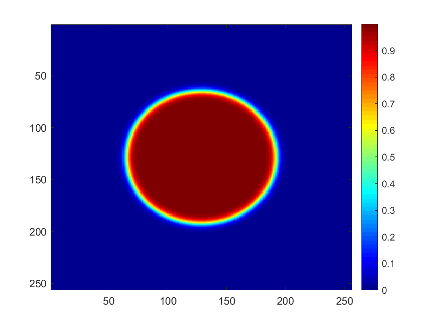
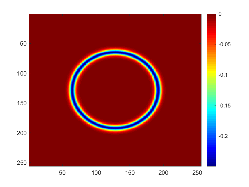
Figure 1. Two phase field representations of the same circle $C$ using the profile $q(t)=\frac{1}{2}(1-\tanh(\frac{t}{2}))$ and its derivative: on the left, $q\left(\frac{d(\cdot,D}{\varepsilon}\right)$ with $D$ the disk enclosed by $C$. On the right, $q^{\prime}\left(\frac{\operatorname{dist}(\cdot,C)}{\varepsilon}\right)$. The first phase field representation carries an orientation information, the second one does not.

Our contribution in this paper is a new class of neural networks aimed to learn, at least approximately, the flow by mean curvature of either oriented or non orientable sets. Since the classical motion by mean curvature of a smooth set can be defined with nonlinear partial differential equations, our contribution falls in the category of learning methods for PDEs. Let us give a brief overview of the literature on neural network-based numerical methods for approximating the solutions to PDEs.

• A first category of approaches relies on the fact that very general functions can be approximated with neural networks [33, 60] so it is natural to seek the solution to a PDE as a neural network  [53, 92, 1, 11, 59, 54]. Such a method is accurate and useful for specific problems, but not convenient: for each new initial condition, a new neural network must be trained. This approach was used for instance in [54] to approximate numerically in high dimension the solutions to nonlinear PDEs with the particular example of the Allen-Cahn equation. It is not well suited to our purposes as it requires at each time to train a new network to produce an approximation of the solution at time $t_{n+1}$ from the solution at time $t_{n}$. In addition, the method requires that the specific structure of the equation is known, which is limited when the underlying equation is only partially known. Another approach considers a neural network as an operator between Euclidean spaces of same dimension depending on the discretization of the PDE [83, 6, 88, 79, 90]. This approach relies on the discretization and requires to modify the architecture of the network when the discrete resolution or the discretization are changed;

• There are strong connections between neural networks and numerical schemes [68, 2, 28, 62]. Most neural networks can actually be seen as operators acting between infinite-dimensional spaces (typically spaces of functions): for instance, for a time-dependent PDE, the forward propagation of an associated neural network can be viewed as the flow associated to the PDE when a time-step $\delta_{t}$ is fixed. Consequently, the neural network is trained only once: for each new initial condition, the solution is obtained by applying the neural network to the initial condition. This reduces significantly the computational cost in comparison with the first category of approaches mentioned above. This second category of approaches is mesh-free and fully data-driven, i.e., the training procedure, as well as the neural network, do not require any knowledge of the underlying PDE, only the knowledge of particular solutions to the PDE. This can be very advantageous when very limited information is given about the PDE, which is often the case in physics. Recently, several works have followed this idea, see [67, 12, 73, 5, 81, 66]. In [67] the authors propose a network architecture based on a theorem of approximation by neural networks of infinite dimensional operators. Very recently, the authors of [66] developed a new neural network based on the Fourier transform. The latter has the advantage of being very simple to implement and computationally very cheap thanks to the Fast Fourier Transform.

• Lastly, there are also methods based on a stochastic approach which uses the links between PDEs and stochastic processes (see [13] and references therein for more details).

The approach proposed in this paper falls in the second category of approaches, i.e., our neural networks approximate the action of semi-group operators for which only few information is known, they are fully data-driven and enough training data is available to get an accurate approximation.

Outline of the paper

The paper is organized as follows: we first present in Section 2 the strategy we adopt for the construction of our numerical schemes based on neural networks. In particular, we introduce the different semigroups involved in our study and detail the whole training protocol starting with the choice of the training data and metrics. The different neural network architectures are described in Section 2, the architectures being inspired by some discretization schemes for the Allen-Cahn equation as in [45, 91]. We focus on two particular networks denoted as $\mathcal{S}^{\text{NN}}_{\theta,1}$ and $\mathcal{S}^{\text{NN}}_{\theta,2}$, and we address in Section 3 their capacity to approximate the mean curvature flows of either oriented or non-orientable surfaces. In the oriented case, we provide some numerical experiments and we give quantitative error estimates to highlight the accuracy and the stability of the numerical schemes associated with our networks. In the non orientable case, both networks seem to learn the flow but a first validation shows that $\mathcal{S}^{\text{NN}}_{\theta,1}$ fails to maintain the evolution of a circle while $\mathcal{S}^{\text{NN}}_{\theta,2}$ succeeds perfectly. To test the reliability of $\mathcal{S}^{\text{NN}}_{\theta,2}$ to approximate the mean curvature flow, evolutions starting from different initial sets are shown in Section 3. We observe in particular that $\mathcal{S}^{\text{NN}}_{\theta,2}$ is able to handle correctly non-orientable surfaces, even with singularities, and the Herring’s condition [20] seems to be respected at points with triple junction. This is somewhat surprising because only evolving smooth sets are used to train our networks (e.g., circles in $2D$, spheres in $3D$). Finally, we propose various applications in Section 4 (multiphase mean curvature flows, Steiner trees, minimal surfaces) to bring out the versatility of our approach and to show that the schemes derived from our trained networks are sufficiently stable to be coupled with additional constraints such as volume conservation or inclusion constraints, and sufficiently stable to be extended to the multiphase case.

2. Neural networks and phase field mean curvature flows

A first possible way, which is not the one we will opt for, to associate neural networks and phase field mean curvature flows is to compute approximations to the solutions of the Allen-Cahn equation (1) by training a neural network $\mathcal{S}^{\mathrm{NN}}_{\theta}$ (depending on a parameter vector $\theta$) to reproduce the action of the Allen-Cahn semigroup $\mathcal{S}^{\text{AC}}_{\delta_{t},\varepsilon}$ defined by

$$\mathcal{S}_{\delta_{t},\varepsilon}^{\text{AC}}[u_{\varepsilon}(\cdot,t)]=u_{\varepsilon}(\cdot,t+\delta_{t}),$$

where $u_{\varepsilon}$ is solution to the Allen-Cahn equation (1) on a set $Q$ with periodic boundary conditions and with constant parameters $\delta_{t}$ and $\varepsilon$.

From this neural network, it is possible to derive the simple numerical scheme

$$u^{n+1}=\mathcal{S}^{\mathrm{NN}}_{\theta}[u^{n}],$$

where the iterate $u^{n}$ is expected to be a good approximation of $u_{\varepsilon}$ at time $t_{n}=n\delta$. However, as explained previously, learning to compute solutions to the Allen-Cahn equation is not necessarily of great interest since extremely simple and robust numerical schemes for computing these solutions already exist.

The idea we propose in this paper is rather to train a network $\mathcal{S}^{\mathrm{NN}}_{\theta}$ to approximate the semigroup $\mathcal{S}^{q}_{\delta_{t},\varepsilon}$ defined by

$$\mathcal{S}^{q}_{\delta_{t},\varepsilon}[v_{\varepsilon}(\cdot,t)]=v_{\varepsilon}(\cdot,t+\delta_{t}),$$

where $v_{\varepsilon}=q\left(\frac{d(x,\Omega(t)}{\varepsilon}\right)$ is an exact phase field representation of an exact mean curvature flow $t\mapsto\Omega(t)$. This second approach is by nature more accurate than the above one since the Allen-Cahn equation is only an approximation to the mean curvature flow whereas $v_{\varepsilon}$ encodes exactly the flow. However, the convergence results of the Allen-Cahn equation to the mean curvature flow show that the two semigroups $\mathcal{S}^{\text{AC}}_{\delta_{t},\varepsilon}$ and $\mathcal{S}^{q}_{\delta_{t},\varepsilon}$ are very close. And since very efficient numerical schemes exist for the Allen-Cahn equation, it makes sense to take inspiration from their structures to design efficient networks.

In a second step, we will adapt our strategy to approximate the mean curvature flow of possibly non-orientable sets by simply replacing the phase field profile $q$. More precisely, we will introduce a network $\mathcal{S}^{\mathrm{NN}}_{\theta}$ to learn an approximation of the semigroup $\mathcal{S}^{q^{\prime}}_{\delta_{t},\varepsilon}$ defined by

$$\mathcal{S}^{q^{\prime}}_{\delta_{t},\varepsilon}[w_{\varepsilon}(\cdot,t)]=w_{\varepsilon}(\cdot,t+\delta_{t}),$$

where $w_{\varepsilon}=q^{\prime}\left(\frac{\text{dist}(x,\Gamma(t))}{\varepsilon}\right)$ with $t\mapsto\Gamma(t)$ the mean curvature flow of a possible non orientable set.

2.1. Training database and loss function

Before providing details about the structure of our neural networks, let us describe the data on which they will be trained and the training energy (the so-called loss function in the literature of neural networks). As before, we shall denote with $t\mapsto\Omega(t)$ the mean curvature flow associated with an initial smooth open set $\Omega(0)$, and with $t\mapsto\Gamma(t)$ the mean curvature flow associated with an initial, possibly non-orientable set $\Gamma(0)$.

Recall that our idea is to obtain an approximation of the operator $\mathcal{S}^{\varphi}_{\delta_{t},\varepsilon}$, where $\varphi=q$ or $\varphi=q^{\prime}$, by training a neural network $S^{\mathrm{NN}}_{\theta}$ on a suitable dataset. We expect that the numerical scheme

$$u^{n+1}=\mathcal{S}^{\mathrm{NN}}_{\theta}[u^{n}]$$

coupled with the initial data

$$u^{0}(x)=\begin{cases}q\left(\frac{d(x,\Omega(0))}{\varepsilon}\right)&\text{ if }\varphi=q,\\ q^{\prime}\left(\frac{\text{dist}(x,\Gamma(0))}{\varepsilon}\right)&\text{ if }\varphi=q^{\prime},\end{cases}$$

will be a good approximation of the mean curvature flows starting from either $\Omega(0)$ or $\Gamma(0)$.

The training of the network $S^{\mathrm{NN}}_{\theta}$ consists in a gradient descent for the parameter vector $\theta$ with respect to a loss energy defined from the exact mean curvature flows of various circles in 2D, of various spheres in 3D, etc.

Let us describe more precisely how the dataset and the associated loss energy are constructed in dimension $d=2$, the construction being similar in higher dimension. Recall that a circle of radius $R_{0}$ evolving under mean curvature flow remains a circle of radius $R(t)=\sqrt{R_{0}^{2}-2t}$ which decreases until the extinction time $T_{R_{0}}=\frac{R_{0}^{2}}{2}$. We select a finite family of radii $R_{i}$ for $i\in\{1,\cdots,N_{\text{train}}\}$ and we define the training dataset as follows:

$$\left\{\left(X_{i},Y_{i}\right)\right\}_{i\in\{1\cdots N_{\text{train}}\}}=\left(\varphi_{R_{i}},\varphi_{\sqrt{R_{i}^{2}-2\delta_{t}}}\right)_{i\in\{1\cdots N_{\text{train}}\}}$$

where

$$\varphi_{R}(x)=\begin{cases}q\left(\frac{\text{d}(x,B_{R})}{\varepsilon}\right)&\text{ if }\varphi=q,\\ q^{\prime}\left(\frac{\text{dist}(x,\partial B_{R})}{\varepsilon}\right)&\text{ if }\varphi=q^{\prime}.\end{cases}$$

with $B_{R}$ the ball of radius $R$ centred at $0$.

We introduce a first loss function:

$$J_{1}(\theta)=\frac{1}{N_{\text{train}}}\sum_{i=1}^{N_{\text{train}}}\|\mathcal{S}^{\mathrm{NN}}_{\theta}[X_{i}]-Y_{i}\|^{2}=\frac{1}{N_{\text{train}}}\sum_{i=1}^{N_{\text{train}}}\int_{Q}\left(\mathcal{S}^{\mathrm{NN}}_{\theta}[\varphi_{R_{i}}]-\varphi_{\sqrt{R_{i}^{2}-2\delta_{t}}}\right)^{2}dx.$$

To stabilize the training of the network $S^{\mathrm{NN}}_{\theta}$, one can opt for a multipoint version which consists in introducing the enriched data set

$$\left\{\left(X_{i},Y_{i,j}\right)\right\}_{\{i\in\{1,\cdots,N_{\text{train}}\},\,j\in\{1,\cdots,k\}\}}=\left(\varphi_{R_{i}},\varphi_{\sqrt{R_{i}^{2}-2j\delta_{t}}}\right)_{\{i\in\{1,\cdots,N_{\text{train}}\},\,j\in\{1,\cdots,k\}\}}$$

and in minimizing the loss functional $J_{k}$ defined by

$$J_{k}(\theta)=\frac{1}{N_{\text{train}}}\sum_{i=1}^{N_{\text{train}}}\sum_{j=1}^{k}\|(\mathcal{S}^{\mathrm{NN}}_{\theta})^{(j)}[X_{i}]-Y_{i,j}\|^{2}=\frac{1}{N_{\text{train}}}\sum_{i=1}^{N_{\text{train}}}\sum_{j=1}^{k}\int_{Q}\left((\mathcal{S}^{\mathrm{NN}}_{\theta})^{(j)}[\varphi_{R_{i}}]-\varphi_{\sqrt{R_{i}^{2}-2j\delta_{t}}}\right)^{2}dx,$$

where $(\mathcal{S}^{\mathrm{NN}}_{\theta})^{(j)}$ is the iterated $j$ times composition of $S^{\mathrm{NN}}_{\theta}$.

In all our experiments, the computational domain is $[0,1]^{d}$ and 2D/3D training data consists of an average of $N_{\text{train}}=100$ circles/spheres with a range of radii ranging from $0.05$ to $0.45$ to capture enough information about the curvatures.

2.2. From the numerical approximation of the Allen-Cahn semigroup to the structure of neural networks

We introduce in this section efficient neural network structures to approximate the semigroups $\mathcal{S}_{\delta_{t},\varepsilon}^{q}$ and $\mathcal{S}_{\delta_{t},\varepsilon}^{q^{\prime}}$. The design of a network architecture is a very delicate question because there is no single generic choice of network that can accurately approximate an operator. The approach developed in this paper consists in deriving the architecture of our networks from splitting methods, which are often used to solve numerically evolution equations having a gradient flow structure. Doing so, we draw on the rich knowledge of numerical analysis to guide us in designing new and more efficient networks.

To derive the structure of our networks, let us start by recalling the principle of splitting schemes [65] to approximate the solutions of the Allen-Cahn equation defined in the domain $Q=[0,1]^{d}$ with periodic boundary conditions (for a recent review of numerical methods for phase field approximation of various geometric flows see [40]). As the two semigroups $S^{\text{AC}}_{\delta_{t},\varepsilon}$ and $\mathcal{S}_{\delta_{t},\varepsilon}^{q}$ are closely related in the case of smooth mean curvature motion, our expectation is that imitating splitting schemes will lead us to very effective networks to approximate first $\mathcal{S}_{\delta_{t},\varepsilon}^{q}$, but also $\mathcal{S}_{\delta_{t},\varepsilon}^{q^{\prime}}$.

Given a time step $\delta_{t}$, we construct an approximation sequence $(u^{n})_{n\geq 0}$ of the solution $u_{\varepsilon}$ of (1) at time $n\delta_{t}$ using various splitting approaches.

First-order neural network $\mathcal{S}^{\text{NN}}_{\theta,1}$
The first splitting method is the semi-implicit approach where the sequence $(u^{n})$ is defined recursively from

$$\frac{u^{n+1}-u^{n}}{\delta_{t}}=\Delta u^{n+1}-\frac{1}{\varepsilon^{2}}W^{\prime}(u^{n}),$$

i.e.,

(4) $$u^{n+1}=\left(I_{d}-\delta_{t}\Delta\right)^{-1}\left(u^{n}-\frac{\delta_{t}}{\varepsilon^{2}}W^{\prime}(u^{n})\right).$$

More precisely, this numerical scheme can be written as a combination of a convolution kernel $K_{1}$ and an activation function $\rho_{1}$:

$$u^{n+1}=K_{1}*\rho_{1}(u^{n}),$$

with $\rho_{1}(s)=s-\frac{\delta_{t}}{\varepsilon^{2}}W^{\prime}(s)$ and

$$K_{1}(x)=\mathcal{F}\left[\xi\mapsto\frac{1}{1+\delta_{t}4\pi^{2}|\xi|^{2}}\right](x),$$

where $\mathcal{F}$ denotes the Fourier transform. This scheme is stable as soon as $\displaystyle\delta_{t}<\sup_{s\in[0,1]}\left\lvert W^{\prime\prime}(s)\right\rvert\varepsilon^{2}$. Moreover, the operator $S^{\text{AC}}_{\delta_{t},\varepsilon,1}:u\mapsto K_{1}*\rho_{1}(u)$ that encodes the semi-implicit scheme can be viewed as an approximation of order $1$ of the Allen-Cahn semigroup $S^{\text{AC}}_{\delta_{t},\varepsilon}$. This method has also the advantage of decoupling the action of the diffusion operator and the reaction operator, therefore each operator can be handled independently.

The previous stability constraint can be avoided using a convex-concave splitting of the Cahn-Hilliard energy. Following the idea introduced by Eyre [45], the functional $P_{\varepsilon}=E_{1}+E_{2}$ is decomposed as the sum of a convex energy $E_{1}$ and a concave energy $E_{2}$ defined by

$$E_{1}(u)=\int_{Q}\left(\varepsilon\frac{|\nabla|^{2}}{2}+\frac{\alpha}{\varepsilon}\frac{u^{2}}{2}\right)dx\quad\text{ and }\quad E_{2}(u)=\frac{1}{\varepsilon}\int_{Q}\left(W(u)-\alpha\frac{u^{2}}{2}\right)dx,$$

with $\alpha$ a sufficiently large stabilization parameter. Treating the convex energy implicitly and the concave energy explicitly yields the scheme

$$u^{n+1}=u^{n}-\frac{\delta_{t}}{\varepsilon}\left(\nabla E_{1}(u^{n+1})+\nabla E_{2}(u^{n})\right),$$

i.e.,

(5) $$u^{n+1}=\left(I_{d}-\delta_{t}\left(\Delta-\frac{\alpha}{\varepsilon^{2}}I_{d}\right)\right)^{-1}\left(u^{n}-\frac{\delta_{t}}{\varepsilon^{2}}(W^{\prime}(u^{n})-\alpha u^{n})\right)=K_{2}*\rho_{2}(u^{n}).$$

Again, this numerical scheme is of the form

$$u^{n+1}=K_{2}*\rho_{2}(u^{n})$$

where the convolution operator $K_{2}$ is now given by

$$K_{2}(x)=\mathcal{F}\left[\xi\mapsto\frac{1}{1+\delta_{t}\left(4\pi^{2}|\xi|^{2}+\frac{\alpha}{\varepsilon^{2}}\right)}\right](x)$$

and the activation function $\rho_{2}$ satisfies $\rho_{2}(s)=s-\frac{\delta_{t}}{\varepsilon^{2}}\left(W^{\prime}(s)-\alpha s\right)$.

The advantage of this scheme is to be unconditionally stable – in the sense that it decreases the Cahn-Hilliard energy – as soon as the stabilization parameter $\alpha$ satisfies $\alpha>\sup_{s\in[0,1]}\left\lvert W^{\prime\prime}(s)\right\rvert=1$ (to be complete, note that choosing a large value for $\alpha$ has also a bad influence on the dynamics of the flow). It is also an approximation of order $1$ to the Allen-Cahn semigroup $\mathcal{S}_{\delta_{t},\varepsilon}^{\mathrm{AC}}$.

This stabilization effect leads us to believe that other such schemes could be obtained by directly learning the diffusion kernel $K$ and the activation function $\rho$ from the training data. The extension to networks is then straightforward since the latter operations can be interpreted as networks. Indeed, the schemes (4) and (5) are reminiscent of the structure of convolutional neural networks (CNN) [64, 69]: a convolution operation coupled with a nonlinear activation function, where the nonlinearity is given by $\rho_{1}$ (or $\rho_{2}$ for (5)) and the learning parameters are the parameters of the kernel associated with the convolution. A first idea of neural network would be to use a CNN with $\rho_{1}$ (for instance) as nonlinearity but it is restrictive because of the choice of $\rho_{1}$ that depends on the parameters $\delta_{t}$ and $\varepsilon$. We propose instead a neural network $\mathcal{S}^{\text{NN}}_{\theta,1}$ constructed as the composition of a pure convolution neuron and a multilayer perceptron (MLP) [85] that will act as a nonlinearity. The network $\mathcal{S}^{\text{NN}}_{\theta,1}$ we propose can be represented by the diagram pictured in figure 2.

Figure 2. Definition of $\mathcal{S}^{\text{NN}}_{\theta,1}$ where $\mathcal{D}$ represents a convolution neuron (or diffusion neuron in reference to diffusion operators), and $\mathcal{R}$ represents a multilayer perceptron (called reaction network in reference to reaction operators). The parameter $\theta$ is the vector of learning parameters, it contains all weights of the $\mathcal{D}$ and $\mathcal{R}$ networks.

The choice of representing the reaction network by a MLP comes from the fact that the action of the reaction operator is totally encoded by a 1D function. According to the fundamental neural network approximation theorem [55, 56, 87] which states that any function can be approximated by a two-layer MLP, it is quite natural to consider a MLP to represent the action of the reaction operator. However, we also choose to use a multilayer perceptron (MLP) as a non-linearity in order to keep some flexibility and not to depend on the context in which we work. The characteristics of the non-linearity are therefore entirely determined during the training stage.

Remark 2.1.

Note that in contrast to the splitting schemes (5) and (4), we have chosen to define the network $\mathcal{S}^{\text{NN}}_{\theta,1}$ by starting with a diffusion neuron $\mathcal{D}$ followed by a non-linearity $\mathcal{R}$ to have a structure similar to the usual convolutional network. The other architecture where we start with $\mathcal{R}$ followed by $\mathcal{D}$ is also very legitimate and gives training results which are similar to those obtained with $\mathcal{S}^{\text{NN}}_{\theta,1}$. However, better numerical results are observed in the test phase when we use $\mathcal{S}^{\text{NN}}_{\theta,1}$ so we shall study only this network.

Higher-order neural networks $\mathcal{S}^{\text{NN}}_{\theta,2}$ and $\mathcal{S}^{\text{NN}}_{\theta,3}$
The network $\mathcal{S}^{\text{NN}}_{\theta,1}$ provides us with the basic block to design more complex and deeper networks as is often the case in deep learning. One can mention, for instance, deep convolutional neural networks (where the basic block is the convolution operation) and deep residual neural networks (with the residual block). Many different networks can derive from $\mathcal{S}^{\text{NN}}_{\theta,1}$. In particular, in order to obtain more complex and effective networks, we now try to adapt the structure of these networks from the higher order semi-implicit schemes developed in [91] in the case of a gradient flow structure. These schemes are structured as follows: starting from $U_{0}=u^{n}$, we set $u^{n+1}=U_{M}$ where $U_{M}$ is defined recursively from $U_{0}$ as

(6) $$U_{m}=U_{0}-\frac{\delta_{t}}{\varepsilon}\left(\sum_{i=0}^{m}\gamma_{i,m}\nabla E_{1}(U_{i})+\sum_{i=0}^{m-1}\tilde{\gamma}_{i,m}\nabla E_{2}(U_{i})\right)\textrm{ for }m=1,\dots,M$$

where the parameters $\gamma_{i,m}$ and $\tilde{\gamma}_{i,m}$ are predefined to ensure the numerical scheme to be highly accurate, see [91] for more information about the choice of the coefficients $\gamma_{i,m}$ and $\tilde{\gamma}_{i,m}$. As can be observed in this scheme (6), the diffusion and reaction operators are applied in chain but also in parallel in order to keep the information of each $U_{i}$ for $i=1,\ldots,M-1$.

The second-order network $\mathcal{S}^{\text{NN}}_{\theta,2}$ which is shown in figure 3 is inspired by the scheme (6) with $M=2$, which reads

$$U_{2}=K_{2}*[\rho_{3}(U_{1})+[U_{0}+\rho_{2}(U_{1})],$$

with $U_{1}=K_{1}*[\rho_{1}(U_{0})]$, and $\gamma_{0,1}=\gamma_{0,2}=\gamma_{0,1}=0$. The curved line in  figure 3, ended by the symbol $\bigoplus$, indicates that the neuron/network $\mathcal{R}$ is equipped with a residual structure in the sense that each entry $u$ to the network $\mathcal{R}$ is added to the output $\mathcal{R}(u)$, i.e. the output of the bottom part of the architecture is $u+\mathcal{R}(u)$. The curved line is actually a skip connection, a technique frequently used in machine learning which consists in skipping one or several layers of a neural network to improve the convergence of the training process by diminishing the effects of vanishing gradients.

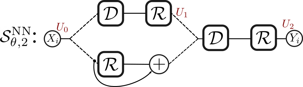
Figure 3. Representation of the 2nd order neural network DR $\mathcal{S}^{\text{NN}}_{\theta,2}$. We adopt the same formalism as for MLPs by assimilating the $\mathcal{D}$ and $\mathcal{R}$ networks to neurons. Here all blocks $\mathcal{D}$ and $\mathcal{R}$ are different, independent networks. The dotted lines mean that the output of the source neuron is multiplied by a weight. The curved line corresponds to a skip connection and indicates that the network $\mathcal{R}$ is equipped with a residual structure.

Remark 2.2.

The residual structure is also a consequence of different experiments we have done where networks with this type of structure had better learning scores and the learning process was faster. In the particular case of the network $\mathcal{S}^{\text{NN}}_{\theta,2}$ we can make the following conjecture: in the classical schemes (4) and (5) reaction operators are related to the double-well potential but also to the phase field profile. In the case of the network $\mathcal{S}^{\text{NN}}_{\theta,2}$, the residual structure allows to maintain this profile after each iteration. Indeed, several recent works [52] highlight the particularity of residual networks to stay close to the inputs by adding the identity.

We can go further in the complexity and the depth of our networks by taking inspiration again from the structure of the scheme (6) with $M=3$. For instance, following the principle of the previous network, we obtain the architecture shown in figure 4.

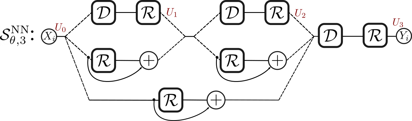
Figure 4. Representation of the 3rd order neural network DR $\mathcal{S}^{\text{NN}}_{\theta,3}$. The same idea used for the structure of the network $\mathcal{S}^{\text{NN}}_{\theta,2}$ is applied to design $\mathcal{S}^{\text{NN}}_{\theta,3}$.

In this paper, we will limit ourselves to the first two networks $\mathcal{S}^{\text{NN}}_{\theta,1}$ and $\mathcal{S}^{\text{NN}}_{\theta,2}$ for the reason that they already give very satisfactory results and it appeared more relevant to us to focus on these first two structures.

2.3. Discretization and specification of our neural networks

In practice, we will consider some approximations of phase field mean curvature flow defined on a square-box $Q=[0,1]^{d}$ using Cartesian grid with $N$ nodes in each direction and using periodic boundary conditions. We consider the approximation parameter $\varepsilon=2/N$ and the fixed timestep $\delta_{t}=\varepsilon^{2}$. Our neural networks are applied to discrete images $U^{n}_{i,j}$ which correspond to a sampling of the function $u^{n}(x_{i,j})$ at the points $x_{i,j}=((i-1)/N,(j-1)/N)$. Our networks depend on the specific choice of the parameters $(\delta_{x},\varepsilon,\delta_{t})$ which have been fixed before the training procedure. In particular, in all the numerical experiments presented below, we set $\delta_{x}=1/N=1/2^{8}$, $\varepsilon=2\delta_{x}$ and $\delta_{t}=\varepsilon^{2}$.

Remark 2.3.

Our approach does not correspond exactly to a method based on neural operators since the definition of the convolutional kernel depends on the discretization in space. It will therefore not be possible to use the trained networks for other choices of discretization parameters. Nevertheless, it is possible to use the trained networks on different sizes of computational box as long as the value of the parameter $\delta_{x}$ remains unchanged. For instance, we can consider a square-box $Q=[0,2]^{d}$ discretized with $N=2^{9}$ nodes in each direction. In this sense, our method remains resolution-invariant thanks to multi-scale techniques.

Diffusional network based on a discrete kernel convolution. 
As $\mathcal{D}$ corresponds to a convolution operation, one needs to specify its hyper-parameters, especially the kernel size $N_{K}$ which is related to the domain discretization and the timestep $\delta_{t}$. In practice, we consider a discrete square kernel $\mathbb{K}$ of size $N_{K}=17$ where the kernel convolution reads as

$$\mathcal{D}[u^{N}]_{\bf k}=(\mathbb{K}*u^{N})_{\boldsymbol{k}}=\sum_{{\boldsymbol{\ell}}\in L_{N}}\mathbb{K}_{\boldsymbol{\ell}}\;u^{N}_{\boldsymbol{k}-\boldsymbol{\ell}}$$

with $L_{N}=[-(N_{K}-1)/2,(N_{K}-1)/2]^{d}$. Here, we assume that the padding extension of $u^{N}$ is periodic. Moreover, the convolution product is computed in practice using the Fast Fourier Transform. Here, recall that the Fourier $\boldsymbol{K}$-approximation of a function $u$ defined in a box $Q=[0,L]^{d}$ is given by

$$u^{\boldsymbol{N}}(x)=\sum_{{\boldsymbol{k}}\in K_{N}}c_{\boldsymbol{k}}e^{2i\pi{\boldsymbol{\xi}}_{k}\cdot x},$$

where $K_{N}=[-\frac{N}{2},\frac{N}{2}-1]^{d}$, ${\boldsymbol{k}}=(k_{1},\dots,k_{d})$ and ${\boldsymbol{\xi}_{k}}=(k_{1}/L,\dots,k_{d}/L)$. In this formula, the $c_{\boldsymbol{k}}$’s denote the $K^{d}$ first discrete Fourier coefficients of $u$. The inverse discrete Fourier transform leads to $u^{N}_{\boldsymbol{k}}=\textrm{IFFT}[c_{\boldsymbol{k}}]$ where $u^{N}_{\boldsymbol{k}}$ denotes the value of $u$ at the points $x_{\boldsymbol{k}}=(k_{1}h,\cdots,k_{d}h)$ and where $h=L/N$. Conversely, $c_{\boldsymbol{k}}$ can be computed as the discrete Fourier transform of $u^{K}_{\boldsymbol{k}},$ i.e., $c_{\boldsymbol{k}}=\textrm{FFT}[u^{N}_{\boldsymbol{k}}].$

Remark 2.4.

In practice, it can be interesting to use kernels with sufficiently small size to facilitate their training but it is necessary to choose a size large enough to avoid anisotropy phenomena due to the square shape of the kernels’ domain.

Remark 2.5.

As we have seen previously, the characteristic size of $\mathbb{K}$ depends strongly on the choice of the time step $\delta_{t}$. In our case, using the time step $\delta_{t}=\epsilon^{2}=(2/N)^{2}$, as shown in figure 5, the support of the heat kernel $K_{\delta_{t}}$ is contained in the interval $[-8/N,8/N]$ which suggests a good approximation by a discrete kernel of size $N_{K}=17$. On the other hand, a time step four times larger $\delta_{t}=4\epsilon^{2}$ would have required a kernel twice as large, i.e., $N_{K}=33$.

      

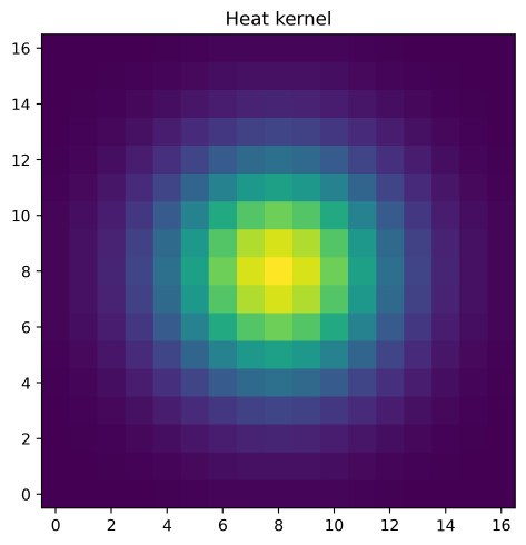
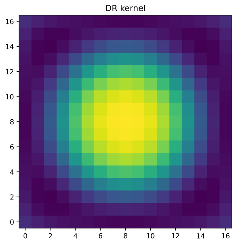
Figure 5. Discrete kernel $\mathbb{K}$. Left: sampling of the heat kernel; Right: example of learned kernel $\mathbb{K}$ for the network $\mathcal{S}^{\text{NN}}_{\theta,1}$ trained to approximate the semigroup $\mathcal{S}_{\varepsilon,\delta_{t}}^{q}$.

Reaction network based on a $1D$ multilayer perceptron  
The reaction network is a multilayer perceptron acting as a function from $\mathbb{R}$ to $\mathbb{R}$. In practice, the number of hidden layers is set to $2$ with $8$ neurons on the first layer and $3$ neurons on the second layer, as pictured in figure 6. By a slight abuse of notation, we denote the same way this network from $\mathbb{R}$ to $\mathbb{R}$ and its action on an image, i.e. we consider that the reaction network applies independently to each component of $u^{N}$:

$$\forall k\in K_{N},\qquad(\mathcal{R}[u^{N}])_{\bf k}=\mathcal{R}[u^{N}_{\bf k}]=\rho{[2]}(W^{[3]}(\rho{[2]}(W^{[2]}(\rho{[1]}(W^{[1]}(u^{N}_{\bf k})+b^{[1]}))+b^{[2]}))+b^{[3]}),$$

where $W^{[1]},b^{[1]},W^{[2]},b^{[2]},W^{[3]},b^{[3]}$ denote the parameters of the network to be optimized and $\rho{[1]},\rho{[2]},\rho{[3]}$ are the three activation functions. Thus, although the reaction neuron is a 1D multilayer perceptron, it extends to an operator that transforms an image into another image of the same size.

We also select the appropriate activation function in the reaction network by testing different choices of activation functions (ReLU, ELU, Sigmoid, SiLU, Tanh, Gaussian) in our numerical experiments. In the end, the Gaussian model seems to have the best properties by presenting more efficient learning rates and speeds.

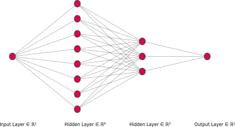
Figure 6. Reaction network based on a $1D$ multilayer perceptron using two hidden layers with respectively $8$ and $3$ neurons.

2.4. Neural network optimization, stopping criteria and Pytorch environment

We now turn to the question of how the learning parameters of our networks are estimated. The learning procedure consists in seeking an optimal vector parameter $\theta$ minimizing the energy $J_{1}$ (or $J_{k},\leavevmode\nobreak\ k>1$ depending on the problem) using a mini-batch stochastic gradient descent algorithm with adaptive momentum [61, 18, 71] on a set of training data.

The reason we use a mini-batch approach is that our problem is a high-dimensional non-convex optimization problem. It is well known that optimizing on mini-batches rather than on the whole dataset reduces the computational cost and the memory cost, and it is commonly used to escape saddle points of the non-convex energy $J_{1}$ (see [51] on this subject).

More precisely, the training strategy is as follows:

Step 1:

Define the neural network $\mathcal{S}_{\theta}$ with the training vector parameter $\theta$.

Step 2:

Generate data using mini-batch: Randomly sample a mini-batch of size $B$ of training labeled couples $(X_{i_{k}},Y_{i_{k}}),\leavevmode\nobreak\ k=1,\cdots,B$ over the training dataset $\{(X_{i},Y_{i})\}_{i=1,\cdots,N_{\mathrm{train}}}$. This means that the training dataset is organized into $N_{\mathrm{train}}/B$ mini-batches and the parameter $\theta$ will be updated for each of these batches. The training batch size $B$ is set to $B=10$ over all experiments. The dataset is reshuffled after every epoch, so that the collection of mini-batches is different at every epoch.

Step 3:

Compute the loss of the mini-batch $J_{1}(\theta)=\displaystyle\frac{1}{B}\sum_{k=1}^{B}\left\|\mathcal{S}_{\theta}[X_{i_{k}}]-Y_{i_{k}}\right\|^{2}$.

Step 4:

Compute the gradient of the previous loss using back-propagation.

Step 5:

Update the learning parameter $\theta$ using the stochastic gradient descent algorithm with adaptive momentum (Adam [61] in our case) and using with the gradient computed at the previous step.

Step 6:

Repeat the steps $2$ to $5$ until all mini-batches have been used. Once all the mini batches have been used, an epoch is said to have passed. In practice, the epoch is set to $\mathrm{epoch}=20000$ for all experiments.

Step 7:

Repeat steps $2$ to $6$ until a stopping criterion is satisfied.

Remark 2.6.

The number of learning parameters of each network is rather small with $N_{\theta}=336$ for the first-order network $\mathcal{S}^{\text{NN}}_{\theta,1}$ and $N_{\theta}=724$ for the second-order network $\mathcal{S}^{\text{NN}}_{\theta,2}$.

Remark 2.7.

Very roughly speaking, stochastic gradient descent algorithms are parametrized by the learning rate, i.e. the step parameter just next to the gradient. The choice of the learning rate is a challenge. Indeed, a too small value may lead to a long training process that could get stuck, while a value that is too large may lead to a selection of sub-optimal learning parameters or an unstable learning process. In practice, schedulers are often used to gradually adjust the learning rate during training. In our case we use the Adam algorithm in step 5 which has the advantage of adjusting the learning rate according to the obtained value of the gradient in step 4.

Remark 2.8.

Regarding the numerical evaluation of the loss function

$${\color[rgb]{0,0,0}J_{1}(\theta)=\frac{1}{N_{\text{train}}}\sum_{i=1}^{N_{\text{train}}}\|\mathcal{S}^{\mathrm{NN}}_{\theta}[X_{i}]-Y_{i}\|^{2}=\frac{1}{N_{\text{train}}}\sum_{i=1}^{N_{\text{train}}}\int_{Q}\left(\mathcal{S}^{\mathrm{NN}}_{\theta}[\varphi_{R_{i}}]-\varphi_{\sqrt{R_{i}^{2}-2\delta_{t}}}\right)^{2}dx,}$$

we observe that all quadrature methods have the same order in periodic boundary conditions, and we opt for the following discretization:

$${\color[rgb]{0,0,0}J^{N}_{1}(\theta)=\frac{1}{N_{\text{train}}}\delta_{x}^{d}\sum_{{\bf k}\in K_{N}}\left(\mathcal{S}^{\mathrm{NN}}_{\theta}[\varphi^{N}_{R_{i}}]_{\bf k}-[\varphi^{N}_{\sqrt{R_{i}^{2}-2\delta_{t}}}]_{\bf k}\right)^{2}.}$$

Checkpointing and selecting criterion

It may happen that after the training process the learning parameters are biased according to the training data. To prevent this and to avoid under- or over-fitting, it is recommended to add an intermediate step during the training procedure. This is called the validation step which consists in evaluating the model on new data (the so-called validation data) and then measuring the error made on these data using one or more metrics. In our case, the validation step is applied at regular intervals every 100 epochs. It is important to note that the parameters of the network are not updated during this procedure.

This step is used as a stopping criterion with the following validation metric which measures the estimation error for the volume of a given sphere evolving by mean curvature. In some sense, this metric is also used to enforce the robustness of the neural network to predict the correct output over several iterations. In practice, the networks parameters which are selected in the end among the parameters saved at each checkpoint are those for which the validation metric gives the best score.

More precisely, the validation metric is given by

$$E_{l}(\theta)=\sum_{i=1}^{l}\sum_{n=0}^{n_{\mathrm{max}}^{i}}\left\lvert\int_{Q}u_{i}^{n}-\int_{Q}\varphi_{\sqrt{R_{i}^{2}-2n\delta_{t}}}\right\rvert^{2},$$

where the sequence $(u_{i}^{n})$ is defined iteratively by

$$\begin{cases}u_{i}^{n+1}&=\mathcal{S}_{\theta}[u_{i}^{n}],\\ u_{i}^{0}&=\varphi_{R_{i}},\end{cases}$$

and $n_{\mathrm{max}}^{i}=\max\{n\in\mathbb{N},\leavevmode\nobreak\ n\delta_{t}<T_{R_{i}}\}$ with $T_{R_{i}}=\frac{R_{i}^{2}}{2}$ the extinction time of the mean curvature flow of the initial sphere of radius $R_{i}$, $i=1,\ldots,l$.

Note that this particular choice of metric stems from the following observation: the evolution of the volume of a sphere with initial radius $R_{0}$ evolving under mean curvature flow is explicitly given by $V(t)=\pi R(t)^{2}=\pi\left(R_{0}^{2}-2t\right)$.

Moreover, if $\varphi=q$, as $\varphi_{R}\approx 1_{B_{R}}$ one can show that

$$\int_{Q}\varphi_{R(t)}=\mathrm{Vol}(B_{R(t)})+\mathcal{O}(\varepsilon^{2})=V(t)+\mathcal{O}(\varepsilon^{2}).$$

In addition, it can also be shown with a similar argument that for $\varphi=-\frac{1}{\varepsilon}q^{\prime}$,

$$\int_{Q}\varphi_{R(t)}=\mathcal{H}^{d-1}(\partial B_{R(t)})+\mathcal{O}(\varepsilon^{2}).$$

In this way, one can see $t\mapsto\int_{Q}\varphi_{R(t)}$ as a good measure of the evolution of the volume (or the perimeter when $\varphi=-\frac{1}{\varepsilon}q^{\prime}$) of a sphere with initial radius $R_{0}$ that evolves by mean curvature flow. In this sense, the energy $E_{l}$ allows to preserve some stability over time (at least on circles or spheres).

All our networks, datasets, visualization tools, etc., have been developed in a Python module dedicated to machine learning for the approximation of interfaces that evolve according to a geometric law (as the mean curvature flow) and are represented by a phase field. This module uses the machine learning framework PyTorch [80] and the high-level interface PyTorch Lightning [46] as the machine learning back-end. For the sake of reproducibility, source codes will be made available at https://github.com/PhaseFieldICJ.

Training computation has been made on a computational server hosted at the Camille Jordan Institute and using a general-purpose graphical processing unit Nvidia V100S. Typical training (20000 epochs) used in the following numerical experiments requires less than 30 minutes of computation without the validation steps.

3. Validation

In this first numerical section, we test the ability of two neural networks to learn either the mean curvature flow $t\mapsto\Omega(t)$ or oriented domains or the mean curvature flow $t\mapsto\Gamma(t)$ of a possible non-orientable sets. These two neural networks are:

• The 1st-order DR network $\mathcal{S}^{\text{NN}}_{\theta,1}$ which combines successively a diffusion neuron and a reaction network.

• The 2nd-order network $\mathcal{S}^{\text{NN}}_{\theta,2}$, which uses two diffusion neurons and three reaction networks, according to the architecture illustrated on figure 3.

More specifically, in each case we will propose a methodology to learn the action of the semigroups $\mathcal{S}_{\delta_{t},\varepsilon}^{q}$ and $S_{\delta_{t},\varepsilon}^{q^{\prime}}$ where the model parameters are set to $\varepsilon=2\delta_{x}$ and $\delta_{t}=\varepsilon^{2}$.

First, the training of the two networks $\mathcal{S}^{\text{NN}}_{\theta,1}$ and $\mathcal{S}^{\text{NN}}_{\theta,2}$ allows us to obtain sufficiently accurate and effective approximations of the semigroup $\mathcal{S}_{\delta_{t},\varepsilon,q}$ to get an approximation of the mean curvature flow of oriented domains whose quality is at least comparable with what would be obtained by solving the Allen-Cahn equation. Going further, a numerical error analysis in the particular case of the evolution of a circle shows that both networks make it possible to reduce the phase field approximation error related to the convergence of the Allen-Cahn equation to the motion by mean curvature in $O(\varepsilon^{2})$.

In the case of the mean curvature flow of possibly non-orientable sets, the first order DR network $\mathcal{S}^{\text{NN}}_{\theta,1}$ fails to learn a sufficiently accurate approximation of the semigroup $\mathcal{S}_{\delta_{t},\varepsilon}^{q^{\prime}}$ and reveals that the basic block architecture DR is not well adapted to this specific setting. On the other hand, the structure of the second order DR network seems much more suitable and provides an interesting approximation of the semigroup $\mathcal{S}_{\delta_{t},\varepsilon}^{q^{\prime}}$ allowing to obtain, at least qualitatively, approximate evolutions of interface under mean curvature flow even in the case of a non-orientable interface $\Gamma$ with multiple junctions.

3.1. Oriented mean curvature flow $t\mapsto\partial\Omega(t)$ and approximation of $S_{\delta_{t},\varepsilon}^{q}$

We now present some preliminary results about the approximation of the semigroup $S_{\delta_{t}=\varepsilon^{2},\varepsilon}^{q}$ based on the training of both neural networks $\mathcal{S}^{\text{NN}}_{\theta,1}$ and $\mathcal{S}^{\text{NN}}_{\theta,2}$ on circles evolving by mean curvature flow and using exact oriented phase field representation. We first plot on figure 7 the evolution of the training loss energy throughout the optimization process, in blue for the network $\mathcal{S}^{\text{NN}}_{\theta,1}$ and in orange for the second one $\mathcal{S}^{\text{NN}}_{\theta,2}$. Clearly, we observe that we manage to learn an approximation of $S_{\delta_{t}=\varepsilon^{2},\varepsilon}^{q}$ with both networks. However, the second order DR network ${}^{\text{NN}}_{\theta,2}$ reaches more quickly acceptable errors on the learning loss, which suggests that the structure of this network is better suited to our problem.

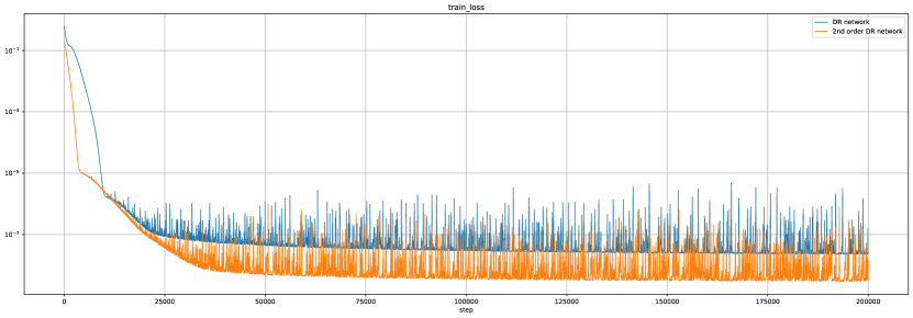
Figure 7. Learning procedure via optimization of the error $J_{1}$ over training data. Training losses of $\mathcal{S}^{\text{NN}}_{\theta,1}$ and $\mathcal{S}^{\text{NN}}_{\theta,2}$ plotted in blue and orange, respectively.

We now want to check that both trained networks achieve accurate approximations of the mean curvature flow. To do so, we test the two associated numerical schemes $u^{n+1}=\mathcal{S}^{\text{NN}}_{\theta,\alpha}[u^{n}]$ with $\alpha\in\{1,2\}$, coupled with an initial condition $u^{0}$ given by $u^{0}=q(d(\Omega_{0},\cdot)/\varepsilon)$ where $\Omega_{0}$ corresponds to a disk of radius $R_{0}=0.3$.

More precisely, we plot in each line of figure 8 the numerical approximation $u^{n}$ obtained at different times $t_{n}=n\delta_{t}$ using respectively the classical Lie splitting scheme $\mathcal{S}^{\text{AC}}_{\delta_{t}=\varepsilon^{2},\varepsilon,1}$, the first order network $\mathcal{S}^{\text{NN}}_{\theta,1}$ and the second order one $\mathcal{S}^{\text{NN}}_{\theta,2}$. All three approximations of the mean curvature flow are so similar that it is difficult to observe any difference between them. At least on this particular example, the networks provide qualitatively the expected evolution.

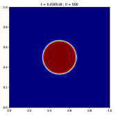
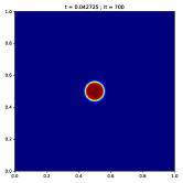
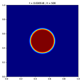
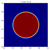
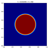
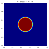
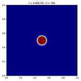
Figure 8. Comparison of the numerical semigroups $\mathcal{S}^{\text{AC}}_{\delta_{t},\varepsilon,1}$, $\mathcal{S}^{\text{NN}}_{\theta,1}$ and $\mathcal{S}^{\text{NN}}_{\theta,2}$ for the approximation of the mean curvature flow of a circle; each row corresponds to the evolution obtained at different times using, respectively, the numerical semigroup $\mathcal{S}^{\text{AC}}_{\delta_{t},\varepsilon,1}$ and the networks $\mathcal{S}^{\text{NN}}_{\theta,1}$ and $\mathcal{S}^{\text{NN}}_{\theta,2}$.

In order to have more quantitative error estimates, we display on figure 9 the error on the integral of the phase field function $\varphi_{R(t)}$ of a circle of radius $R(t)$ during the iterations knowing that the evolution by mean curvature of an initial disk of radius $R_{0}$ is a disk of radius $R(t)=\sqrt{R_{0}^{2}-2t}$, at least until the extinction time $t_{0}=\frac{1}{2}R_{0}^{2}$. More precisely, we plot:

• the volume error

  $${\color[rgb]{0,0,0}n\mapsto\left|\int_{Q}u^{n}(x)dx-\int_{Q}\varphi_{\sqrt{R_{0}^{2}-2n\delta_{t}}}(x)dx\right|^{2}},$$

• the (squared) $L^{2}$ error

  $${\color[rgb]{0,0,0}n\mapsto\int_{Q}\left(u^{n}(x)-\varphi_{\sqrt{R_{0}^{2}-2n\delta_{t}}}(x)\right)^{2}dx,}$$

using

• the trained network $\mathcal{S}^{\text{NN}}_{\theta,1}$ in blue

• the trained network $\mathcal{S}^{\text{NN}}_{\theta,2}$ in orange

• the Lie splitting scheme $\mathcal{S}^{\text{AC}}_{\delta_{t},\varepsilon,1}$ with $\delta_{t}=\epsilon^{2}$ in green

• the Lie splitting scheme $\mathcal{S}^{\text{AC}}_{\delta_{t},\varepsilon,1}$ with $\delta_{t}=\epsilon^{2}/10$ in red

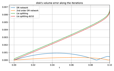
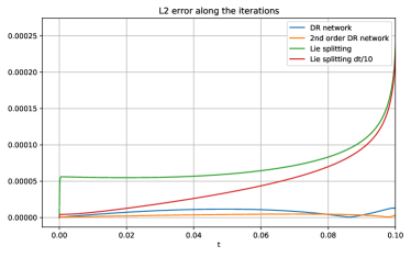
Figure 9. Comparison of different schemes on the evolution of a disk by approximate mean curvature flow with initial radius $R_{0}=0.45$. Plots in blue, orange, green, and red correspond to the error along iterations of, respectively, the trained networks $\mathcal{S}^{\text{NN}}_{\theta,1}$ and $\mathcal{S}^{\text{NN}}_{\theta,2}$, and the schemes $\mathcal{S}^{\text{AC}}_{\delta_{t}=\varepsilon^{2},\varepsilon,1}$ and $\mathcal{S}^{\text{AC}}_{\delta_{t},\varepsilon,1}$ with $\delta_{t}=\epsilon^{2}/10$. Left : disk’s volume error, Right : $L^{2}$ error.

These results clearly show that both our neural networks $\mathcal{S}^{\text{NN}}_{\theta,1}$ and $\mathcal{S}^{\text{NN}}_{\theta,2}$ provide more accurate numerical schemes than the classical discretization of the Allen-Cahn equation, even using a smaller time step $\delta_{t}$.

This first validation test shows also that the training of our networks manages to correct both the errors of discretization of the Allen-Cahn equation, and the modeling errors of the approximation by the Allen-Cahn equation of the mean curvature flow.

We now repeat the experiment considering instead a starting radius $R_{0}$ which does not belong to the training interval $[0.05,0.45]$. This will be useful in assessing the ability of our neural networks to generalize well, i.e to handle properly new configurations which are not in the training database. We use a twice as large computational domain $Q=[0,2]^{2}$ which can contain an initial circle of radius $R_{0}=0.75$. We use the same networks as before without requiring any re-training. As the parameters $\delta_{x}$, $\varepsilon$ and $\delta_{t}$ are fixed, observe that due to the visualization scale, the width of the diffuse interface is twice as small on each image of figure 10 in comparison with figure 8. In figure 11 we plot the volume error along iterations associated with the estimated radius $R(t)$ for each method. As observed previously, the second order network $S^{NN}_{2,\theta}$ is the most accurate method, although its performance has marginally deteriorated as compared to the previous experiment. Still, these results confirm that our networks generalize well.

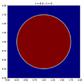
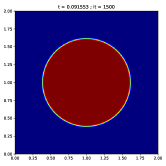
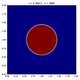
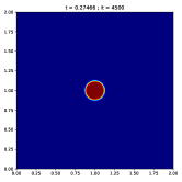
Figure 10. Evolution along the iterations starting from an initial circle of radius $R_{0}=0.75$ on a domain $Q$ twice as large using the network $\mathcal{S}^{\text{NN}}_{\theta,1}$.

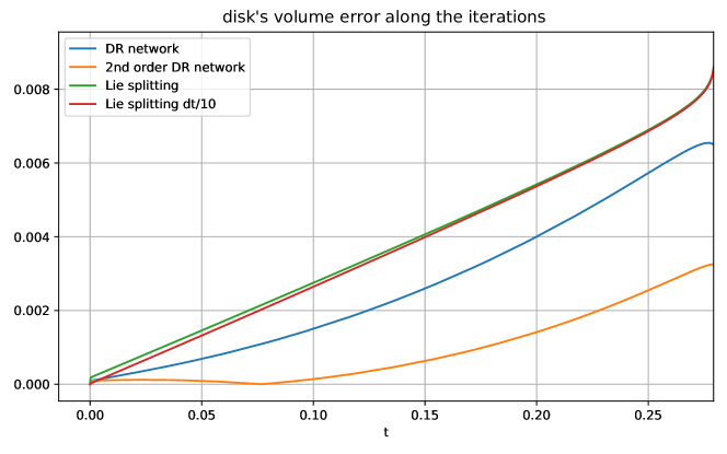
Figure 11. Comparison of different schemes on the evolution of the radius of a circle with initial radius $R_{0}=0.75$ evolving by mean curvature flow. Plots in blue, orange, green, and red correspond to the error $n\mapsto\left(\int_{Q}u^{n}(x)dx-\int_{Q}\varphi_{\sqrt{R_{0}^{2}-2n\delta_{t}}}(x)dx\right)^{2}$ along iterations of, respectively, the trained networks $\mathcal{S}^{\text{NN}}_{\theta,1}$ and $\mathcal{S}^{\text{NN}}_{\theta,2}$, and the schemes $\mathcal{S}^{\text{AC}}_{\delta_{t}=\varepsilon^{2},\varepsilon,1}$ and $\mathcal{S}^{\text{AC}}_{\delta_{t},\varepsilon,1}$ with $\delta_{t}=\epsilon^{2}/10$.

We plot in figure 12 a last numerical comparison in the case of a non-convex initial set $\Omega(0)$ and, as before, we can clearly observe that the flows are qualitatively very similar.

In conclusion, the use of neural networks not only allows us to obtain good approximations of the mean curvature motion but, as shown by the quantitative comparisons above, these approximations are also of better quality than what can be obtained using a phase field approach and a solution to the Allen-Cahn equation.

These results are therefore very encouraging and show even more the interest of neural networks for phase field approximations in the even worser case where the models would not be as accurate as the Allen-Cahn equation or the numerical schemes would not be as efficient or accurate.

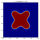
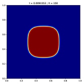
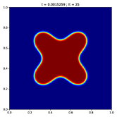
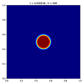
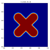
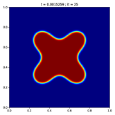
Figure 12. Comparison of numerical semigroups $\mathcal{S}^{\text{AC}}_{\delta_{t},\varepsilon,1}$, $\mathcal{S}^{\text{NN}}_{\theta,1}$ and $\mathcal{S}^{\text{NN}}_{\theta,2}$ to approximate the mean curvature flow of a non convex initial set; each line corresponds respectively to the evolution obtained at different times $t$ using, respectively, the numerical semigroups $\mathcal{S}^{\text{AC}}_{\delta_{t},\varepsilon,1}$, $\mathcal{S}^{\text{NN}}_{\theta,1}$ and $\mathcal{S}^{\text{NN}}_{\theta,2}$.

3.2. Non orientable mean curvature flow $t\mapsto\Gamma(t)$ and approximation of $S_{\delta_{t},\varepsilon}^{q^{\prime}}$

Let us describe some numerical results on the approximation of the $S_{\delta_{t},\varepsilon}^{q^{\prime}}$ semigroup, still using the same architecture for the two neural networks $\mathcal{S}^{\text{NN}}_{\theta,1}$ and $\mathcal{S}^{\text{NN}}_{\theta,2}$ but training on data built from evolutions of circles in the exact non-oriented phase field representation. Let us recall here that to the limit of our knowledge, there is no phase field model allowing to approximate such a flow by solving an Allen-Cahn-type PDE. As before, the idea is to train both our networks on a database still made of circles evolution on a $\delta_{t}$ time step, but using the $q^{\prime}$ profile instead of $q$.

We first plot in figure 13 the evolution of the training loss energy during the training process, respectively in blue and orange for the networks $\mathcal{S}^{\text{NN}}_{\theta,1}$ and $\mathcal{S}^{\text{NN}}_{\theta,2}$. Here, both networks seem to succeed in learning the flow, although the train loss value seems much better for the second network $\mathcal{S}^{\text{NN}}_{\theta,2}$.

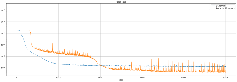
Figure 13. Learning process by optimizing the training losses $J_{k}$ with $k=5$ for the networks $\mathcal{S}^{\text{NN}}_{\theta,1}$ and $\mathcal{S}^{\text{NN}}_{\theta,2}$, respectively plotted in blue and orange.

In contrast, when we test both networks to approximate the motion by the mean curvature of a circle, we clearly observe on figure 14 that the first order network $\mathcal{S}^{\text{NN}}_{\theta,1}$ does not manage to keep the profile $q^{\prime}$ in a stable way and to decrease the radius of the circle. The good news is that the second network $\mathcal{S}^{\text{NN}}_{\theta,2}$ leads to a numerical scheme that is stable enough to reproduce well the evolution of the circle while keeping the $q^{\prime}$ profile along the evolution. In order to have a more quantitative criterion on the evolution of the circle, we draw on figure 15 the evolution $n\mapsto\pi(\frac{1}{2\pi\varepsilon}\int u^{n}(x)dx)^{2}$ which should correspond to the evolution of the area of a circle of radius $R(t)$ given by $t\mapsto\pi(R_{0}^{2}-2t)$. This is indeed clearly the case on figure 15 which shows that the obtained evolution law corresponds well to the motion by mean curvature.

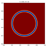
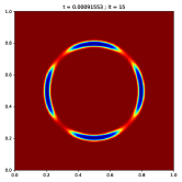
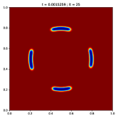
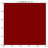
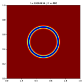
Figure 14. Numerical comparison of networks $\mathcal{S}^{\text{NN}}_{\theta,1}$ and $\mathcal{S}^{\text{NN}}_{\theta,2}$ to approximate the mean curvature flow of a circle in the non oriented setting; each row corresponds to the evolution obtained at different times using $\mathcal{S}^{\text{NN}}_{\theta,1}$ and $\mathcal{S}^{\text{NN}}_{\theta,2}$, respectively.

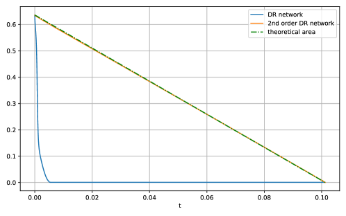
Figure 15. Comparison of different schemes on the evolution of the radius of a circle evolving by mean curvature flow. Plots in blue, orange correspond to $n\mapsto\pi(\frac{1}{2\pi\varepsilon}\int u^{n}(x)dx)^{2}$ along iterations using respectively $\mathcal{S}^{\text{NN}}_{\theta,1}$ and $\mathcal{S}^{\text{NN}}_{\theta,2}$. In green, the theoretical evolution of the circle area $n\mapsto\pi(R_{0}^{2}-2n\delta_{t})$.

In order to test the reliability of the network $\mathcal{S}^{\text{NN}}_{\theta,2}$ to approximate motions by mean curvature in a general way, we also compare the evolution obtained with the scheme deriving from our network with the one deriving from the discretization of the Allen-Cahn equation.

Here, although the starting set $\Omega(0)$ is the same in both numerical experiments, the initial phase field solution $u^{0}$ is different and depends on the profile used. We plot on figure 16 the solution $u^{n}$ computed at different times $t_{n}$ using either the Allen-Cahn discrete semigroup $\mathcal{S}^{\text{AC}}_{\delta_{t}=\varepsilon^{2},\varepsilon,1}$ or the network $\mathcal{S}^{\text{NN}}_{\theta,2}$. We clearly observe a similar flow that validates the methodology and the use of our neural networks to approximate the motion by mean curvature in the case of a non-orientable set.

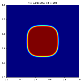
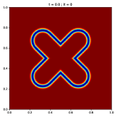
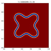
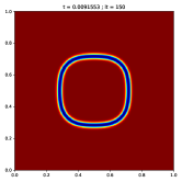
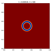
Figure 16. Approximation of the mean curvature flow of a non convex initial set: numerical comparison of the classical discretisation of the Allen-Cahn equation $\mathcal{S}^{\text{AC}}_{\delta_{t}=\varepsilon^{2},\varepsilon,1}$ (first line) with the network $\mathcal{S}^{\text{NN}}_{\theta,2}$ trained on the non oriented phase field $q^{\prime}(\operatorname{dist}(x,\Gamma)/\varepsilon)$ (second line). In each line, we plot the solution $u^{n}$ at different times $t_{n}$.

We also plot on figure 17 the numerical approximation of the mean curvature flow obtained in the case of non-orientable initial sets. In each of these experiments, we observe the evolution of points with triple junction which seem to satisfy the Herring condition [20]. This result is all the more surprising since our training base contained only circle evolutions and no interface with the triple point. The presence of stable triple points is therefore very good news and shows the potential of this approach for the general case of mean curvature motion.

We give a last example in figure 18 of an approximation of mean curvature flow in the case of an initial non-closed interface. Here the example is quite pathological since it is very difficult to make sense of the motion by mean curvature, and we expect the interface to disappear in infinitesimal time. Surprisingly, the evolution seems relatively stable with a speed of the endpoints of the order of $1/\varepsilon$ (which is consistent with the $O(1)$ speed at regular points of the circle).

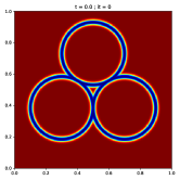
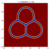
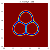
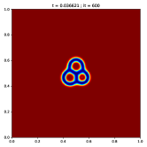
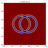
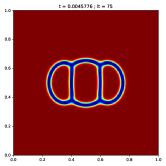
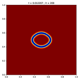
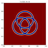
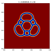
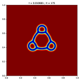
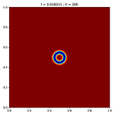
Figure 17. Approximation of the mean curvature flow of a non orientable initial set. Each line corresponds to a different choice of the initial set $\Gamma(0)$. We display the solution $u^{n}$ at different times $t_{n}$ along the iterations.

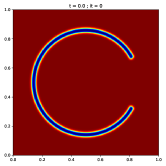
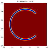
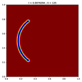
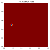
Figure 18. Approximation of the motion by mean curvature of an initial open curve.

4. Applications: multiphase mean curvature flows, Steiner trees, and minimal surfaces

We highlight in this section how the previous schemes derived from our trained networks $S^{NN}_{\theta,\alpha},\leavevmode\nobreak\ \alpha\in\{1,2\}$, are sufficiently stable to be coupled with additional constraints such as volume conservation ($\int_{Q}u^{n}dx$ constant) or inclusion constraints (reformulated as an inequality $u^{n}\geq u_{in}(x)$, see [21]), and sufficiently stable to be extended to the multiphase case.

Instead of retraining the networks for these applications, we simply use the same networks trained earlier on circles and spheres, and we couple their predictions with an additional constraint in a post-processing step to approximate the solution. Doing so, we demonstrate the adaptability of our neural network approach.

Partition problem in dimension $2$. The first application concerns the approximation of multiphase mean curvature flow with or without volume conservation. We recall that the evolution of a partition with $N$ phases ${\bf\Omega(t)}=(\Omega_{1}(t),\Omega_{2}(t),\cdots\Omega_{N}(t))$ can be obtained as the $L^{2}$-gradient flow of a multiphase perimeter

$${\color[rgb]{0,0,0}P({\bf\Omega})=\frac{1}{2}\sum_{i=1}^{N}P(\Omega_{i})=\frac{1}{2}\sum_{i=1}^{N}\int_{\partial\Omega_{i}}d\mathcal{H}^{1}},$$

with the normal velocity $V_{i,j}$ of each interface $\Gamma_{i,j}=\partial\Omega_{i}\cap\partial\Omega_{j}$ satisfying

$$V_{i,j}=H_{i,j},$$

where $H_{i,j}$ represents the mean curvature at the interface $\Gamma_{i,j}$.

The Steiner problem in dimension $2$. The second application is the approximation of Steiner trees in dimension $2$, i.e. solutions of the Steiner problem. Recall that the Steiner problem consists, given a collection of points $a_{1},\ldots,a_{L}\in\Omega$, in finding a compact connected set $K\subset\Omega$ containing all the $a_{i}$’s and having minimal length. In other words, it is equivalent to finding the optimal solution to the following problem

$$\min\left\{\mathcal{H}^{1}(K),\leavevmode\nobreak\ K\subset\Omega,K\text{ connected, }a_{i}\in K,\leavevmode\nobreak\ \forall i=1,\cdots,L\right\},$$

where $\mathcal{H}^{1}(K)$ corresponds to the one-dimensional Hausdorff measure of $K$. As the optimal set $K$ needs not be orientable, our idea is to combine the network $S^{NN}_{\theta,2}$ trained on the non-oriented phase field database with the inclusion constraints associated to all points $a_{i}$’s.

The Plateau problem in dimension $3$. The last application focuses on the Plateau problem in dimension $3$ and co-dimension $1$. Recall that it consists in finding, for a given closed boundary curve $\Gamma$, a compact set $E$ in $\Omega$ with minimal area and whose boundary coincides with $\Gamma$ [34]. In other words, it amounts to solving the minimization problem

(7) $$\min\{\mathcal{H}^{2}(E);E\subset\Omega,\text{connected and such as }\partial E=\Gamma\},$$

where $\mathcal{H}^{2}(E)$ stands for the two-dimensional Hausdorff measure of $E$. Analogously to the method proposed for the Steiner problem, the approximation method we propose consists in

1. training a $S^{NN}_{\theta,2}$ network on databases built from $3D$ spheres evolving under mean curvature flow with a non-oriented phase field representation,

2. coupling the trained network $S^{NN}_{\theta,2}$ with the inclusion constraint to force the boundary constraint $\partial E=\Gamma$.

4.1. Evolution of a partition in dimension $2$

As explained previously, the motivation in this first application is to approximate multiphase mean curvature flows. Recall that the phase field approach consists in general [50, 49, 47, 78, 23] in introducing a multiphase field function ${\bf u}=(u_{1},u_{2},\cdots,u_{N})$, solution of an Allen-Cahn system obtained as the $L^{2}$-gradient flow of the multiphase Cahn-Hilliard energy $P_{\varepsilon}$ defined by

$$P_{\varepsilon}({\bf u})=\begin{cases}{\color[rgb]{0,0,0}\frac{1}{2}\sum_{k=1}^{N}\int_{Q}\frac{\varepsilon}{2}|\nabla u_{k}|^{2}+\frac{1}{\varepsilon}W(u_{k})dx}&\text{ if }\sum_{k=1}^{N}u_{k}=1,\\ +\infty&\text{ otherwise.}\end{cases}$$

More precisely, the Allen-Cahn system [22, 20] reads as

$$\partial_{t}u_{k}=\Delta u_{k}-\frac{1}{\varepsilon^{2}}W^{\prime}(u_{k})+\lambda\sqrt{2W(u_{k})},\quad k=1,\cdots,N$$

where the Lagrange multiplier $\lambda$ is associated with the partition constraint $\sum_{k=1}^{L}u_{k}=1$. As explained in [22, 20], this PDE can be for instance computed in two steps:

1. Solve the decoupled Allen-Cahn system

   $$u_{k}^{n+1/2}=\mathcal{S}^{\text{AC}}_{\delta_{t},\varepsilon,1}[u_{k}^{n}],\quad k=1,\cdots,N.$$

2. Project onto the partition constraint $\sum_{k}u_{k}^{n+1}=1$:

   $$u_{k}^{n+1}=u_{k}^{n+1/2}+\lambda^{n+1}\sqrt{2W(u_{k}^{n+1/2})},\quad k=1,\cdots,N.$$

   Notice that the Lagrange multiplier $\lambda^{n+1}$ is computed following the expression

   $$\lambda^{n+1}=\frac{1-\sum_{k=1}^{N}u_{k}^{n+1/2}}{\sum_{k=1}^{N}\sqrt{2W(u_{k}^{n+1/2})}},$$

   in order to satisfy exactly the partition constraint.

This discretization scheme associated with the Allen-Cahn system suggests to simply replace the Lie splitting Allen-Cahn operator $\mathcal{S}^{\text{AC}}_{\delta_{t},\varepsilon,1}$ by our network $\mathcal{S}^{NN}_{\theta,1}$ trained on oriented mean curvature flow in section (3.1). A numerical experiment obtained with such a strategy is presented on the first row of figure 19. More precisely, we consider here an evolution of a multiphase system with four phases and we observe at least qualitatively that the flow seems to be correct with a triple junction forming angles of $2\pi/3$. The second row of figure 19 gives a similar numerical experiment with additional constraint on the volume of each phase. Here, following the approach developed in [48, 74, 19, 22], the idea is to consider the Allen-Cahn system with volume conservation

$$\partial_{t}u_{k}=\Delta u_{k}-\frac{1}{\varepsilon^{2}}W^{\prime}(u_{k})+\lambda\sqrt{2W(u_{k})}+\mu_{k}\sqrt{2W(u_{k})},$$

where the new Lagrange multiplier $\mu_{k}$ is defined to satisfy $\mathrm{Vol}_{k}=\int_{Q}u_{k}=\int_{Q}u_{0}$. The previous scheme can then be modified by considering now a projection on the partition and the volume constraints as

$$u_{k}^{n+1}=u_{k}^{n+1/2}+(\lambda^{n+1}+\mu_{k}^{n+1})\sqrt{2W(u_{k}^{n+1/2})},$$

where the Lagrange multipliers $(\lambda^{n+1},\mu_{1}^{n+1},\mu_{2}^{n+1},\cdots\mu_{N}^{n+1})$ are for instance given by

$$\mu_{k}^{n+1}=\frac{\mathrm{Vol}_{k}-\int_{Q}u^{n+1/2}_{k}}{\int_{Q}\sqrt{2W(u_{k}^{n+1/2}})},\text{ and }\lambda^{n+1}=\frac{1-\sum_{k=1}^{N}\left[u_{k}^{n+1/2}+\mu_{k}^{n+1}\sqrt{2W(u_{k}^{n+1})}\right]}{\sum\sqrt{2W(u_{k}^{n+1/2})}},$$

which allows each of the constraints to be satisfied. As previously, the idea consists simply to replace the Lie splitting Allen-Cahn operator $\mathcal{S}^{\text{AC}}_{\delta_{t},\varepsilon_{1}}$ by our network $\mathcal{S}^{NN}_{\theta,1}$. In particular, the numerical experiment plotted on the second row of figure 19 shows a stable multiphase evolution where the volume of each phase seems to be conserved. These two numerical examples clearly show that our networks previously trained on mean curvature motion flow can be re-exploited in more complex situations.

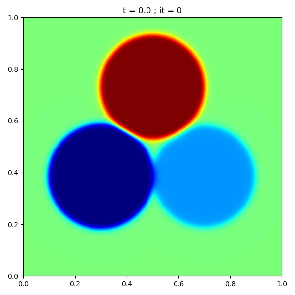
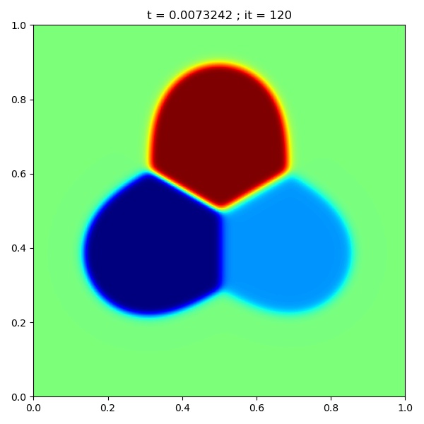
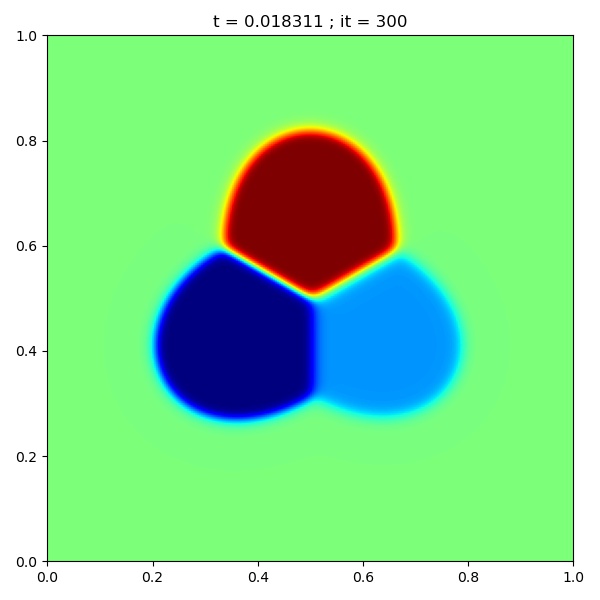
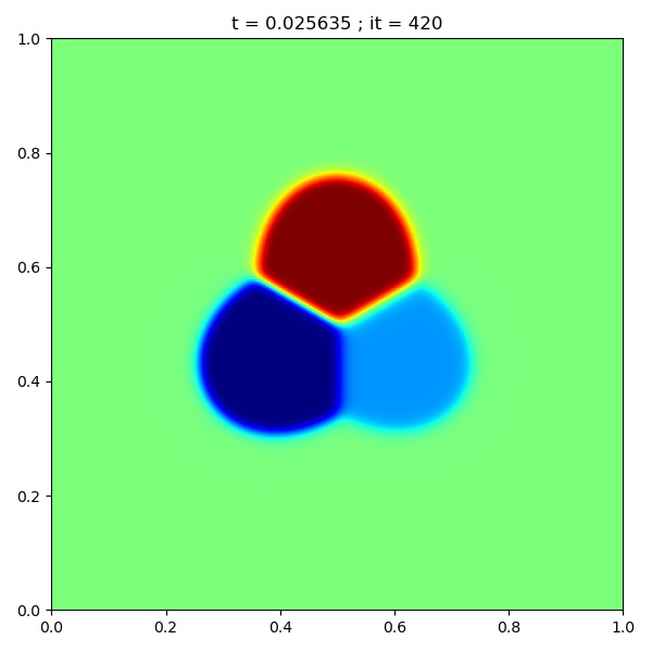
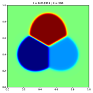
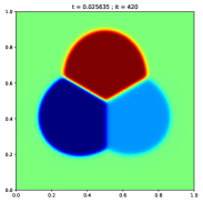
Figure 19. Mean curvature flows of three interconnecting circles without (first row) and with (second row) additional volume constraint.

4.2. Approximation of Steiner trees in $2D$

Variational phase field models have been recently introduced [17, 16, 14, 15, 26] to tackle the Steiner problem. For example, the model introduced in [17] proposes the Ambrosio-Tortorelli functional

$$F_{\varepsilon}(u)=\int_{{\color[rgb]{0,0,0}\Omega}}\varepsilon|\nabla u|^{2}+\frac{1}{\varepsilon}(1-u)^{2}dx,$$

coupled with an additional penalization term $G_{\varepsilon}(u)$ which forces the connectedness of the set $K$ and which is defined by

$$G_{\varepsilon}(u)=\frac{1}{\varepsilon}\sum_{i=1}^{N}{\bf D}(u^{2};a_{0},a_{i}),\text{ with }{\bf D}(w;a,b):=\inf_{\Gamma:a\leadsto b}\int_{\Gamma}w\,d\mathcal{H}^{1}\in[0,+\infty],$$

where the notation $\Gamma:a\leadsto b$ means that $\Gamma$ is a rectifiable curve in $\Omega$ connecting $a$ and $b$.

Intuitively, the phase field function $u_{\varepsilon}$ is expected to be of the form $u_{\varepsilon}=\varphi(\operatorname{dist}(x,K)/\varepsilon)$, the Ambrosio-Torterelli term approximates the length of $K$, and the geodesic term $G_{\varepsilon}$ forces the solution $u_{\varepsilon}$ to vanish on $K$, and $K$ to connect the different points $a_{i}$. An analysis of this model and, more precisely, a $\Gamma$-convergence result established in [17] suggest that the minimization of this phase field model should give an approximation of a Steiner solution, i.e. a Steiner tree. However, numerical experiments as proposed in [17] and in [16] show the ability of this coupling to approximate solutions of the Steiner problem in dimensions $2$ and $3$ but show also all the difficulties to minimize efficiently the geodesic term $G_{\varepsilon}$ to preserve the connectedness of the set $K$. The conclusions are quite similar for the approaches developed in [14, 15, 26] where the idea is rather to use the measure-theoretic notion of current and the connectedness of the set $K$ is ensured by adding a divergence constraint of the form $div(\tau)=\sum\alpha_{i}\delta_{a_{i}}$.

We propose a completely different approach by considering a non oriented mean curvature flow $t\mapsto\Gamma(t)$ of an initial connected set $\Gamma(0)$ containing all the points $a_{i}$ coupled with the additional inclusion constraint $\{a_{i},\leavevmode\nobreak\ i=1,\cdots,N\}\subset\Gamma(t)$. Indeed, we expect that the stationary state of such an evolution is at least a local minimum of the Steiner problem. From a phase field point of view, the strategy is to consider the non-oriented phase field representation $q^{\prime}(\operatorname{dist}(x,\Gamma(t)/\varepsilon))$, to use the non oriented trained network $\mathcal{S}^{NN}_{\theta,2}$ to let the interface evolve by mean curvature, and to incorporate the inclusion constraint by using an additional inequality constraint

$$u\leq u_{\text{in}}(x)=\sum_{i=1}^{N}q^{\prime}(\operatorname{dist}(a_{i},x)/\varepsilon),$$

in the spirit of [24, 21]. Finally, the scheme reads as follows:

1. Approximation of a non-oriented mean curvature flow step

   $$u^{n+1/2}=\mathcal{S}^{\text{NN}}_{\theta,2}[u^{n}].$$

2. Projection on the inclusion constraint $u\leq u_{\text{in}}(x)$:

   $${u^{n+1}}=\text{min}(u_{\text{in}},u^{n+1/2}).$$

We present in figure 20 three numerical experiments using, respectively, $4$, $5$, and $6$ points $a_{i}$ arranged non-uniformly on a circle. The first picture of each line corresponds to the initial set $\Gamma(0)$ constructed in such a way to connect the point $a_{1}$ in a linear way to all other points $a_{i}$, ${i\in\{2\cdots N\}}$. We then clearly observe an evolution of the set $\Gamma(t)$ which seems to converge to a Steiner tree connecting all points $a_{i}$. In particular, the triple points seem to be handled accurately enough. In the end, the method seems extremely effective, simple to implement, and the computation of Steiner solutions is really fast compared to other methods proposed in the literature. These results illustrate that our network trained on non-oriented mean curvature flows has sufficient numerical stability properties to be coupled with inclusion constraints.

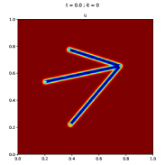
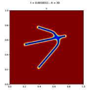
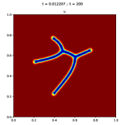
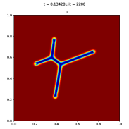
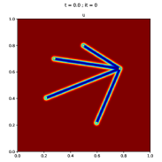
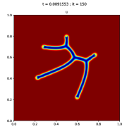
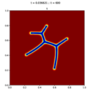
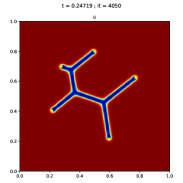
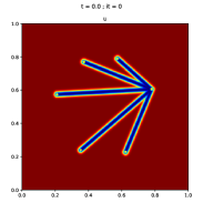
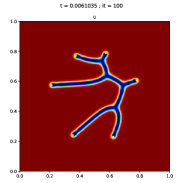
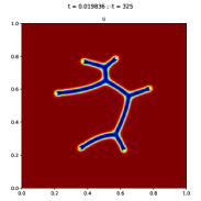
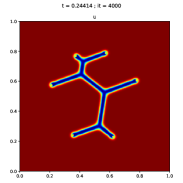
Figure 20. Approximation of Steiner trees in $2D$ using a non oriented mean curvature flow coupled with inclusion constraints according to the scheme (4.2); Each line shows an evolution of the numerical solution $u^{n}$ along the iterations with, respectively, $4$, $5$, and $6$ points $a_{i}$.

4.3. Approximation of minimal surfaces in $3D$

The Plateau problem was formulated by Lagrange in 1760 and consists in showing the existence of a minimal surface in $\mathbb{R}^{3}$ with prescribed boundary $\Sigma$. Existence and regularity of solutions have been studied in different contexts, see for instance [39] for smooth and orientable solutions and [84] for existence and uniqueness of soap films including orientable and non orientable surfaces and possibly multiple junctions.

From the numerical point of view, there exist many methods to compute minimal surfaces, as for instance the first one [38] and others [89, 32] which use a parametric representation of the surface. In the same spirit, the papers [41, 42] exploit a finite element method to compute numerical approximations of minimal surfaces. Finally, note also some numerical approaches using an implicit representation of the minimal surface in [31, 25] where a level set method is used. As for phase field approaches, a current-based method was proposed and analyzed in [27], and provides numerical approximations in the case of oriented surfaces.

We propose in this section to extend to $3D$ the phase field approach used for the Steiner problem. The idea is very similar in the sense that

1. We train a new network $\mathcal{S}^{NN}_{\theta,2}$ to approximate the semigroup $S_{\delta_{t},\varepsilon,q^{\prime}}$ in dimension $3$. Here we consider the case of the mean curvature flow of co-dimension $1$. The training of the network is performed on a database consisting of spheres involving under motion by mean curvature which is also explicit in this case.

2. We apply the previous scheme where the function $u_{in}$ is now defined by

   $$u_{\text{in}}(x)=\sum_{i=1}^{N}q^{\prime}(\operatorname{dist}(\Sigma,x)/\varepsilon).$$

We present in figures 21 and 22 four numerical experiments using respectively the boundary of a Mobius strip, a trefunknot, a union of rings, and a pit. The prescribed boundary $\Sigma$ and the boundary of $\{x\in Q;u_{n}(x)\geq-0.2\}$ are respectively plotted in red and green along the iterations. We display in figure 21 the evolution of an interface along the iterations toward the stationary numerical solution. We show in figure 22 only the stationary solutions, i.e. the minimal surfaces associated with the respective prescribed boundaries.

These numerical results are very encouraging because they are examples of non-orientable solutions with more or less complex topologies, and possibly with triple line singularities.

Note that the results obtained with our neural networks are perfectly consistent with those obtained using other methods, see for instance [16] for Steiner 2D trees and [57] for minimal surfaces.

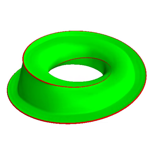
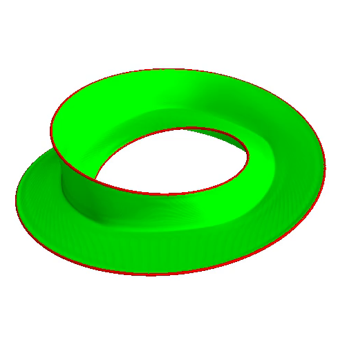
Figure 21. Approximation of a minimal surface using a non-oriented mean curvature flow coupled with an inclusion constraint. The images represent the numerical solution $u^{n}$ at four different times. The prescribed boundary $\Sigma$ and the boundary of $\{x\in Q;u_{n}(x)\geq-0.2\}$ are plotted in red and green, respectively .

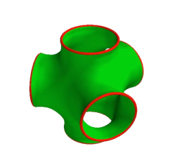
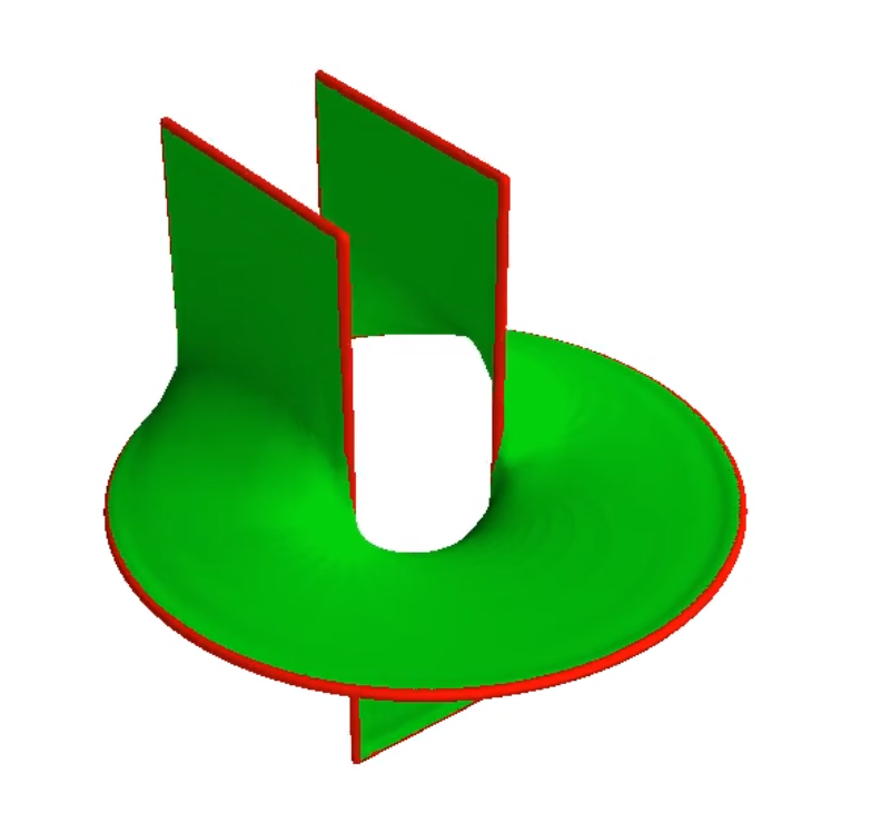
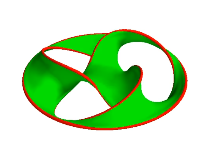
Figure 22. Approximation of minimal surfaces using a non-oriented mean curvature flow coupled with an inclusion constraint; Each picture shows the numerical stationary solution $u^{n}$ in green and the prescribed boundary $\Sigma$ in red.

5. Conclusion

We have introduced in this work neural networks that provide simple and very effective numerical schemes to accurately approximate motions by mean curvature in the classical case of oriented interfaces, as well as in the case of non orientable interfaces for which classical phase field approaches are not suitable. The structures of our networks are inspired by discretization schemes of the Allen-Cahn equation that alternate linear diffusion and local nonlinear reaction. Our networks are very effective despite their low number of degrees of freedom (less than 1000) compared to standard networks such as U-net which has millions of parameters. This low complexity facilitates faster training and enforces robustness. This is best illustrated by the ability of our networks to generalize well despite a limited and simplistic training database. The first numerical results presented in this paper are very encouraging. In particular, the application to the Plateau problem of our numerical method based on neural networks shows that it can well approximate non-orientable minimal surfaces with triple junction lines. It is quite reasonable to expect that our approach can be extended to many other interface geometric flows, e.g., anisotropic mean curvature motion, surface diffusion, the Willmore flow, etc., possibly with various constraints. Furthermore, our approach seems quite generic and possible extension is expected to more general diffusion-reaction equations and the rich world of associated applications. Lastly, since the network structures we propose can be easily coupled with constraints, it would be interesting to explore further in the near future the coupling with constraints such as bounds on solutions or the positivity of convolution kernels to ensure the monotonicity of the associated numerical schemes.

References

- [1] J. Adler and O. Öktem. Solving ill-posed inverse problems using iterative deep neural networks. Inverse Problems, 33(12):124007, 2017.
- [2] T. Alt, K. Schrader, M. Augustin, P. Peter, and J. Weickert. Connections between numerical algorithms for PDEs and neural networks. arXiv preprint arXiv:2107.14742, 2021.
- [3] L. Ambrosio. Geometric evolution problems, distance function and viscosity solutions. In Calculus of variations and partial differential equations (Pisa, 1996), pages 5–93. Springer, Berlin, 2000.
- [4] L. Ambrosio and V. M. Tortorelli. Approximation of functionals depending on jumps by elliptic functionals via -convergence. Comm. Pure Appl. Math., 43(8):999–1036, 1990.
- [5] A. Anandkumar, K. Azizzadenesheli, K. Bhattacharya, N. Kovachki, Z. Li, B. Liu, and A. Stuart. Neural operator: Graph kernel network for partial differential equations. In ICLR 2020 Workshop on Integration of Deep Neural Models and Differential Equations, 2020.
- [6] L. Bar and N. Sochen. Unsupervised deep learning algorithm for PDE-based forward and inverse problems, arxiv. arXiv preprint arXiv:1904.05417, 2019.
- [7] J. W. Barrett, H. Garcke, and R. Nürnberg. On the parametric finite element approximation of evolving hypersurfaces in . J. Comput. Phys., 227:4281–4307, April 2008.
- [8] G. Bellettini. Lecture notes on mean curvature flow, barriers and singular perturbations, volume 12 of Appunti. Scuola Normale Superiore di Pisa (Nuova Serie) [Lecture Notes. Scuola Normale Superiore di Pisa (New Series)]. Edizioni della Normale, Pisa, 2013.
- [9] G. Bellettini and M. Paolini. Quasi-optimal error estimates for the mean curvature flow with a forcing term. Differential and Integral Equations, 8(4):735–752, 1995.
- [10] J. Bence, B. Merriman, and S. Osher. Diffusion generated motion by mean curvature. Computational Crystal Growers Workshop,J. Taylor ed. Selected Lectures in Math., Amer. Math. Soc., pages 73–83, 1992.
- [11] S. Bhatnagar, Y. Afshar, S. Pan, K. Duraisamy, and S. Kaushik. Prediction of aerodynamic flow fields using convolutional neural networks. Computational Mechanics, 64(2):525–545, 2019.
- [12] K. Bhattacharya, B. Hosseini, N. B. Kovachki, and A. M. Stuart. Model reduction and neural networks for parametric PDEs. arXiv preprint arXiv:2005.03180, 2020.
- [13] J. Blechschmidt and O. G. Ernst. Three ways to solve partial differential equations with neural networks—a review. GAMM-Mitteilungen, page e202100006, 2021.
- [14] M. Bonafini, G. Orlandi, and E. Oudet. Variational approximation of functionals defined on 1-dimensional connected sets: the planar case. SIAM J. Math. Anal., 50(6):6307–6332, 2018.
- [15] M. Bonafini and E. Oudet. A convex approach to the Gilbert-Steiner problem. Interfaces Free Bound., 22(2):131–155, 2020.
- [16] M. Bonnivard, E. Bretin, and A. Lemenant. Numerical approximation of the Steiner problem in dimension 2 and 3. Math. Comp., 89(321):1–43, 2020.
- [17] M. Bonnivard, A. Lemenant, and F. Santambrogio. Approximation of length minimization problems among compact connected sets. SIAM J. Math. Anal., 47(2):1489–1529, 2015.
- [18] L. Bottou. Large-scale machine learning with stochastic gradient descent. In Proceedings of COMPSTAT’2010, pages 177–186. Springer, 2010.
- [19] M. Brassel and E. Bretin. A modified phase field approximation for mean curvature flow with conservation of the volume. Mathematical Methods in the Applied Sciences, 34(10):1157–1180, 2011.
- [20] E. Bretin, A. Danescu, J. Penuelas, and S. Masnou. Multiphase mean curvature flows with high mobility contrasts: a phase-field approach, with applications to nanowires. Journal of Computational Physics, 365:324–349, 2018.
- [21] E. Bretin, F. Dayrens, and S. Masnou. Volume reconstruction from slices. SIAM J. Imaging Sci., 10(4):2326–2358, 2017.
- [22] É. Bretin, R. Denis, J.-O. Lachaud, and É. Oudet. Phase-field modelling and computing for a large number of phases. ESAIM: M2AN, 53(3):805–832, 2019.
- [23] E. Bretin and S. Masnou. A new phase field model for inhomogeneous minimal partitions, and applications to droplets dynamics. Interfaces and Free Boundaries, 19(2):141–182, 2017.
- [24] E. Bretin and V. Perrier. Phase field method for mean curvature flow with boundary constraints. ESAIM Math. Model. Numer. Anal., 46(6):1509–1526, 2012.
- [25] T. Cecil. A numerical method for computing minimal surfaces in arbitrary dimension. J. Comput. Phys., 206(2):650–660, 2005.
- [26] A. Chambolle, L. A. D. Ferrari, and B. Merlet. A phase-field approximation of the Steiner problem in dimension two. Adv. Calc. Var., 12(2):157–179, 2019.
- [27] A. Chambolle, L. A. D. Ferrari, and B. Merlet. Variational approximation of size-mass energies for -dimensional currents. ESAIM Control Optim. Calc. Var., 25:Paper No. 43, 39, 2019.
- [28] A. Chambolle and T. Pock. Learning consistent discretizations of the total variation. SIAM Journal on Imaging Sciences, 14(2):778–813, 2021.
- [29] X. Chen. Generation and propagation of interfaces in reaction-diffusion systems. Transactions of the American Mathematical Society, 334(2):877–913, 1992.
- [30] Y. G. Chen, Y. Giga, and S. Goto. Uniqueness and existence of viscosity solutions of generalized mean curvature flow equations. Proc. Japan Acad. Ser. A Math. Sci., 65(7):207–210, 1989.
- [31] D. L. Chopp. Computing minimal surfaces via level set curvature flow. J. Comput. Phys., 106(1):77–91, 1993.
- [32] C. Coppin and D. Greenspan. A contribution to the particle modeling of soap films. Appl. Math. Comput., 26(4):315–331, 1988.
- [33] G. Cybenko. Approximation by superpositions of a sigmoidal function. Mathematics of Control, Signals, and Systems (MCSS), 2(4):303–314, Dec. 1989.
- [34] G. David. Should we solve Plateau’s problem again? Lecture for the conference in Honor of E. Stein, 2011, July 2012.
- [35] P. De Mottoni and M. Schatzman. Geometrical evolution of developed interfaces. Transactions of the American Mathematical Society, 347(5):1533–1589, 1995.
- [36] K. Deckelnick, G. Dziuk, and C. M. Elliott. Computation of geometric partial differential equations and mean curvature flow. Acta Numer., 14:139–232, 2005.
- [37] K. Deckelnick, G. Dziuk, and C. M. Elliott. Computation of geometric partial differential equations and mean curvature flow. Acta Numer., 14:139–232, 2005.
- [38] J. Douglas. A method of numerical solution of the problem of Plateau. Ann. of Math. (2), 29(1-4):180–188, 1927/28.
- [39] J. Douglas. Solution of the problem of Plateau. Trans. Amer. Math. Soc., 33(1):263–321, 1931.
- [40] Q. Du and X. Feng. Chapter 5 - The phase field method for geometric moving interfaces and their numerical approximations. In A. Bonito and R. H. Nochetto, editors, Handbook of Numerical Analysis, volume 21 of Geometric Partial Differential Equations - Part I, pages 425–508. Elsevier, 2020-01-01.
- [41] G. Dziuk and J. E. Hutchinson. The discrete Plateau problem: algorithm and numerics. Math. Comp., 68(225):1–23, 1999.
- [42] G. Dziuk and J. E. Hutchinson. The discrete Plateau problem: convergence results. Math. Comp., 68(226):519–546, 1999.
- [43] S. Esedoḡlu and F. Otto. Threshold dynamics for networks with arbitrary surface tensions. Comm. Pure Appl. Math., 68(5):808–864, 2015.
- [44] L. C. Evans and J. Spruck. Motion of level sets by mean curvature. I. J. Differential Geom., 33(3):635–681, 1991.
- [45] D. J. Eyre. Unconditionally gradient stable time marching the Cahn-Hilliard equation. MRS Online Proceedings Library Archive, 529, 1998/ed.
- [46] W. Falcon et al. Pytorch lightning. GitHub. Note: https://github. com/PyTorchLightning/pytorch-lightning, 3:6, 2019.
- [47] H. Garcke and R. Haas. Modelling of non-isothermal multi-component, multi-phase systems with convection. Technical report, 2008.
- [48] H. Garcke, B. Nestler, B. Stinner, and F. Wendler. Allen-Cahn systems with volume constraints. Math. Models Methods Appl. Sci., 18(8):1347–1381, 2008.
- [49] H. Garcke, B. Nestler, and B. Stoth. On anisotropic order parameter models for multi-phase systems and their sharp interface limits. Physica D: Nonlinear Phenomena, 115(1-2):87 – 108, 1998.
- [50] H. Garcke, B. Nestler, and B. Stoth. A multi phase field concept: Numerical simulations of moving phase boundaries and multiple junctions. SIAM J. Appl. Math, 60:295–315, 1999.
- [51] R. Ge, F. Huang, C. Jin, and Y. Yuan. Escaping from saddle points—online stochastic gradient for tensor decomposition. In Conference on learning theory, pages 797–842. PMLR, 2015.
- [52] K. Greff, R. K. Srivastava, and J. Schmidhuber. Highway and residual networks learn unrolled iterative estimation. arXiv preprint arXiv:1612.07771, 2016.
- [53] X. Guo, W. Li, and F. Iorio. Convolutional neural networks for steady flow approximation. In Proceedings of the 22nd ACM SIGKDD international conference on knowledge discovery and data mining, pages 481–490, 2016.
- [54] J. Han, A. Jentzen, and W. E. Solving high-dimensional partial differential equations using deep learning. Proc. Natl. Acad. Sci. USA, 115(34):8505–8510, 2018.
- [55] K. Hornik. Approximation capabilities of multilayer feedforward networks. Neural networks, 4(2):251–257, 1991.
- [56] K. Hornik. Some new results on neural network approximation. Neural networks, 6(8):1069–1072, 1993.
- [57] C.-K. Huang. Questions of approximation and compactness for geometric variational problems. Phd thesis, Université de Lyon, Oct 2021.
- [58] H. Ishii, G. E. Pires, and P. E. Souganidis. Threshold dynamics type approximation schemes for propagating fronts. J. Math. Soc. Japan, 51(2):267–308, 1999.
- [59] Y. Khoo, J. Lu, and L. Ying. Solving parametric PDE problems with artificial neural networks. European Journal of Applied Mathematics, 32(3):421–435, 2021.
- [60] P. Kidger and T. Lyons. Universal Approximation with Deep Narrow Networks. In J. Abernethy and S. Agarwal, editors, Proceedings of Thirty Third Conference on Learning Theory, volume 125 of Proceedings of Machine Learning Research, pages 2306–2327. PMLR, 09–12 Jul 2020.
- [61] D. P. Kingma and J. Ba. Adam: A method for stochastic optimization. arXiv preprint arXiv:1412.6980, 2014.
- [62] E. Kobler, T. Klatzer, K. Hammernik, and T. Pock. Variational networks: Connecting variational methods and deep learning. In V. Roth and T. Vetter, editors, Pattern Recognition, pages 281–293, Cham, 2017. Springer International Publishing.
- [63] T. Laux and F. Otto. Convergence of the thresholding scheme for multi-phase mean-curvature flow. Calc. Var. Partial Differential Equations, 55(5):Art. 129, 74, 2016.
- [64] Y. LeCun, B. Boser, J. Denker, D. Henderson, R. Howard, W. Hubbard, and L. Jackel. Handwritten digit recognition with a back-propagation network. In D. Touretzky, editor, Advances in Neural Information Processing Systems, volume 2. Morgan-Kaufmann, 1989.
- [65] H. G. Lee and J.-Y. Lee. A semi-analytical Fourier spectral method for the Allen–Cahn equation. Computers & Mathematics with Applications, 68(3):174–184, Aug. 2014.
- [66] Z. Li, N. Kovachki, K. Azizzadenesheli, B. Liu, K. Bhattacharya, A. Stuart, and A. Anandkumar. Fourier neural operator for parametric partial differential equations. arXiv preprint arXiv:2010.08895, 2020.
- [67] L. Lu, P. Jin, and G. E. Karniadakis. Deeponet: Learning nonlinear operators for identifying differential equations based on the universal approximation theorem of operators. arXiv preprint arXiv:1910.03193, 2019.
- [68] Y. Lu, A. Zhong, Q. Li, and B. Dong. Beyond finite layer neural networks: Bridging deep architectures and numerical differential equations. In International Conference on Machine Learning, pages 3276–3285. PMLR, 2018.
- [69] S. Mallat. Understanding deep convolutional networks. Philosophical Transactions of the Royal Society A: Mathematical, Physical and Engineering Sciences, 374(2065):20150203, 2016.
- [70] C. Mantegazza, M. Novaga, and A. Pluda. Lectures on curvature flow of networks. In Contemporary research in elliptic PDEs and related topics, volume 33 of Springer INdAM Ser., pages 369–417. Springer, Cham, 2019.
- [71] D. Masters and C. Luschi. Revisiting small batch training for deep neural networks. arXiv preprint arXiv:1804.07612, 2018.
- [72] L. Modica and S. Mortola. Un esempio di -convergenza. Boll. Un. Mat. Ital. B (5), 14(1):285–299, 1977.
- [73] N. H. Nelsen and A. M. Stuart. The random feature model for input-output maps between banach spaces. SIAM Journal on Scientific Computing, 43(5):A3212–A3243, 2021.
- [74] B. Nestler, F. Wendler, M. Selzer, B. Stinner, and H. Garcke. Phase-field model for multiphase systems with preserved volume fractions. Phys. Rev. E, 78:011604, Jul 2008.
- [75] S. Osher and R. Fedkiw. Level Set Methods and Dynamic Implicit Surfaces. Springer-Verlag New York, Applied Mathematical Sciences, 2002.
- [76] S. Osher and N. Paragios. Geometric Level Set Methods in Imaging, Vision and Graphics. Springer-Verlag, New York, 2003.
- [77] S. Osher and J. A. Sethian. Fronts propagating with curvature-dependent speed: algorithms based on hamilton-jacobi formulations. J. Comput. Phys., 79:12–49, 1988.
- [78] E. Oudet. Approximation of partitions of least perimeter by Gamma-convergence: around Kelvin’s conjecture. Experimental Mathematics, 20(3):260–270, 2011.
- [79] S. Pan and K. Duraisamy. Physics-informed probabilistic learning of linear embeddings of nonlinear dynamics with guaranteed stability. SIAM Journal on Applied Dynamical Systems, 19(1):480–509, 2020.
- [80] A. Paszke, S. Gross, F. Massa, A. Lerer, J. Bradbury, G. Chanan, T. Killeen, Z. Lin, N. Gimelshein, L. Antiga, A. Desmaison, A. Kopf, E. Yang, Z. DeVito, M. Raison, A. Tejani, S. Chilamkurthy, B. Steiner, L. Fang, J. Bai, and S. Chintala. Pytorch: An imperative style, high-performance deep learning library. In Advances in Neural Information Processing Systems 32, pages 8024–8035. Curran Associates, Inc., 2019.
- [81] R. G. Patel, N. A. Trask, M. A. Wood, and E. C. Cyr. A physics-informed operator regression framework for extracting data-driven continuum models. Computer Methods in Applied Mechanics and Engineering, 373:113500, 2021.
- [82] P. Pozzi and B. Stinner. On motion by curvature of a network with a triple junction. The SMAI journal of computational mathematics, 7:27–55, 2021.
- [83] M. Raissi, P. Perdikaris, and G. E. Karniadakis. Physics-informed neural networks: A deep learning framework for solving forward and inverse problems involving nonlinear partial differential equations. Journal of Computational Physics, 378:686–707, 2019.
- [84] E. R. Reifenberg. Solution of the Plateau problem for -dimensional surfaces of varying topological type. Bull. Amer. Math. Soc., 66:312–313, 1960.
- [85] F. Rosenblatt. The perceptron: a probabilistic model for information storage and organization in the brain. Psychological review, 65(6):386, 1958.
- [86] S. J. Ruuth. Efficient algorithms for diffusion-generated motion by mean curvature. J. Comput. Phys., 144(2):603–625, 1998.
- [87] F. Scarselli and A. C. Tsoi. Universal approximation using feedforward neural networks: A survey of some existing methods, and some new results. Neural networks, 11(1):15–37, 1998.
- [88] J. D. Smith, K. Azizzadenesheli, and Z. E. Ross. Eikonet: Solving the eikonal equation with deep neural networks. IEEE Transactions on Geoscience and Remote Sensing, 59:10685–10696, 2021.
- [89] H.-J. Wagner. A contribution to the numerical approximation of minimal surfaces. Computing, 19(1):35–58, 1977/78.
- [90] B. Yu. The deep Ritz method: A deep learning-based numerical algorithm for solving variational problems, commun. math. Stat, 6:1–12, 2018.
- [91] A. Zaitzeff, S. Esedoḡlu, and K. Garikipati. High order, semi-implicit, energy stable schemes for gradient flows. Journal of Computational Physics, 447:110688, 2021.
- [92] Y. Zhu and N. Zabaras. Bayesian deep convolutional encoder–decoder networks for surrogate modeling and uncertainty quantification. Journal of Computational Physics, 366:415–447, 2018.