Theory-experiment comparison for the Casimir force between metallic test bodies: A spatially nonlocal dielectric response

Abstract

It has been known that the Lifshitz theory of the Casimir force comes into conflict with the measurement data if the response of conduction electrons in metals to electromagnetic fluctuations is described by the well tested dissipative Drude model. The same theory is in a very good agreement with measurements of the Casimir force from graphene whose spatially nonlocal electromagnetic response is derived from the first principles of quantum electrodynamics. Here, we propose the spatially nonlocal phenomenological dielectric functions of metals which lead to nearly the same response, as the standard Drude model, to the propagating waves, but to a different response in the case of evanescent waves. Unlike some previous suggestions of this type, the response functions considered here depend on all components of the wave vector as is most natural in the formalism of specular reflection used. It is shown that these response functions satisfy the Kramers-Kronig relations. We derive respective expressions for the surface impedances and reflection coefficients. The obtained results are used to compute the effective Casimir pressure between two parallel plates, the Casimir force between a sphere and a plate, and its gradient in configurations of the most precise experiments performed with both nonmagnetic (Au) and magnetic (Ni) test bodies. It is shown that in all cases (Au-Au, Au-Ni, and Ni-Ni test bodies) the predictions of the Lifshitz theory found by using the dissipative nonlocal response functions are in as good agreement with the measurement data, as was reached previously with the dissipationless plasma model. Possible developments and applications of these results are discussed.

I Introduction

As predicted by Casimir 1 , two parallel uncharged ideal metal planes separated by a distance $a$ at zero temperature should attract each other by the force

$$F(a)=-\frac{\pi^{2}}{240}\,\frac{\hbar c}{a^{4}},$$ (1)

which depends on the Planck constant $\hbar$ and the speed of light $c$. According to Casimir, this force is caused by the zero-point oscillations of quantized electromagnetic field whose spectrum is altered by the presence of ideal metal planes. Within the formalism of quantum electrodynamics, in the absence of planes the zero-point energy is given by an integral over a continuous wave vector $k$. In the presence of planes, however, the tangential component of electric field vanishes on the plane surfaces and the component $k_{z}$ in direction perpendicular to the planes becomes discrete. The modified zero-point energy of the electromagnetic field is an integral over $k_{x}$ and $k_{y}$, but a discrete sum in $k_{z}$. Although both zero-point energies in the absence and in the presence of planes are infinitely large, their difference is finite. As a result, the negative derivative of this difference with respect to $a$ is equal to the Casimir force (1).

More recently, it was understood that the Casimir force, as well as the more familiar van der Waals force, belongs to a wide class of physical phenomena determined by the zero-point and thermal fluctuations of the electromagnetic field. Lifshitz 2 created the general theory of forces of this kind acting between two parallel material plates (semispaces) kept at any temperature in thermal equilibrium with the environment. In the framework of the Lifshitz theory, the ideal metal boundary conditions are replaced by the electrodynamic continuity conditions which take into account real material properties by means of the frequency-dependent dielectric permittivity and (for magnetic plates) magnetic permeability.

There are two main approaches to a derivation of basic expressions of the Lifshitz theory for the free energy and force of fluctuation origin. One of them is based on the fluctuation-dissipation theorem of statistical physics 2 ; 3 and another one, which goes back to Casimir, on quantum field theory with appropriate boundary conditions 4 ; 5 ; 6 ; 7 . By the frequently used present-day terminology, the name van der Waals force refers to the fluctuation-induced forces at separations of a few nanometers which do not depend on $c$. The term Casimir force is used in all remaining cases, i.e., when the interaction of fluctuation origin depends on $\hbar$, $c$, material properties and temperature. By now the Lifshitz theory is generalized for the case of boundary surfaces of arbitrary geometric shape 8 ; 9 ; 10 ; 11 ; 12 .

A systematic investigation of the thermal Casimir force between parallel plates made of real metals traces back to 2000. In Ref. 13 it was shown that if the low-frequency dielectric response of metals is described by the realistic Drude model taking a proper account of the relaxation properties of conduction electrons, the Lifshitz theory predicts large thermal correction which arises at short separations of a few hundred nanometers at room temperature and decreases the force magnitude. The thermal correction of this type does not arise if the low-frequency dielectric response of metals is described by the plasma model which disregards the relaxation properties of conduction electrons 14 . It should be remembered, however, that the plasma model is in fact applicable only at high frequencies in the range of infrared optics where the relaxation properties do not play any role. The surprising thing is that the Casimir entropy calculated with the Lifshitz theory employing the Drude model violates the third law of thermodynamics (the Nernst heat theorem) for metals with perfect crystal lattices 15 ; 16 ; 17 ; 18 ; 19 ; 20 ; 21 (the Nernst heat theorem is followed for metals with the defects of structure 22 ; 23 ; 24 , but this does not solve the problem because perfect crystal lattice is a system with the nondegenerate ground state, so that it should satisfy the third law of thermodynamics). If, however, the Casimir entropy is found using the plasma model dielectric response, the Nernst heat theorem is satisfied without trouble 15 ; 16 ; 17 ; 18 ; 19 ; 20 ; 21 .

Of even greater surprise is that the theoretical predictions of the Lifshitz theory using the Drude dielectric response at low frequencies have been excluded by the measurement data of many experiments performed with both nonmagnetic (Au) and magnetic (Ni) metallic test bodies by the two different experimental groups 25 ; 26 ; 27 ; 28 ; 29 ; 30 ; 31 ; 32 ; 33 ; 34 ; 35 ; 36 ; 37 . The same measurement data were found to be in a very good agreement with the predictions of the Lifshitz theory employing the plasma dielectric response 25 ; 26 ; 27 ; 28 ; 29 ; 30 ; 31 ; 32 ; 33 ; 34 ; 35 ; 36 ; 37 . In the most striking experiment of Ref. 33 using the differential measurement scheme, a difference between the excluded and confirmed theoretical predictions was by up to a factor of 1000. Thus, the Drude mode, which provides an adequate description of numerous optical and electrical physical phenomena, does not work in application to the Casimir force.

Note that the measurement data of one experiment performed at separations of a few micrometers were found to be in better agreement with theoretical predictions using the Drude model 38 . To obtain this conclusion, the Casimir force calculated using the Drude or the plasma model was subtracted from by the order of magnitude larger measured force. The obtained differences were fitted to the theoretical electric force originating from the surface patches. The results of Ref. 38 were shown to be, however, uncertain because in this experiment the surface imperfections, which are unavoidably present on a surface of the used spherical lens of centimeter-size radius, were ignored 39 . Recent Casimir experiment performed in the micrometer separation range, where the patch potentials were directly measured by means of Kelvin probe microscopy, demonstrated an agreement with theoretical predictions using the plasma model and excluded those using the Drude model 37 .

An apparent disagreement of theoretical predictions of the fundamental Lifshitz theory using the Drude model, which was fully validated in the area of electromagnetic and optical phenomena other than the Casimir effect, with the measurement data, as well as with the basic principles of thermodynamics, is puzzling and calls for a satisfactory explanation. This subject was hotly debated in the literature starting from 2000 and many attempts have been made directed to reaching an agreement with thermodynamics, looking for some unaccounted systematic effects in measurements of the Casimir force, or developing the more exact theory for a sphere-plate geometry used in experiments. Considerable advances have been made in this way (see Refs. 40 ; 41 ; 42 ; 43 ; 44 ; 45 for a review), but the ultimate resolution of the Casimir puzzle still remains to be found.

One possible approach to understanding of this problem is that all models of the electromagnetic response of macroscopic bodies are in some sense phenomenological, either relying on assumptions about bulk properties or upon very simplified models of the response of individual atoms to an applied field. This means that no model derived in any macroscopic framework using, e.g., the Boltzmann transport equations or Kubo theory can be expected to work under all circumstances, especially, in the very extreme conditions in Casimir force experiments. From this standpoint, it is not at all surprising that some physical situations give results in contrast with the predictions of commonly used models. There are, however, some limitations following from fundamental physics that exacerbate the situation. Thus, according to Maxwell equations, the dielectric response of metals to electromagnetic field in the quasistatic limit is inverse proportional to the frequency. The Drude model satisfies this demand and describes the relaxation properties of conduction electrons whereas the dielectric permittivity of the plasma model is inverse proportional to the second power of frequency and does not describe the relaxation properties.

At one time it was hoped that a resolution of this problem may come from the investigation of graphene which is a two-dimensional sheet of carbon atoms packed in the hexagonal crystal lattice. At energies below a few eV, which are characteristic for the Casimir effect at not too short separations, graphene is well described by the Dirac model as a set of massless or very light electronic quasiparticles satisfying the Dirac equation where $c$ is replaced with the Fermi velocity $v_{\,\rm F}$ 46 ; 47 . The spatially nonlocal dielectric response of graphene to electromagnetic field was found precisely on the basis of first principles of quantum electrodynamics using the polarization tensor 48 ; 49 ; 50 ; 51 . The Lifshitz theory employing this dielectric response turned out to be in agreement with experiments on measuring the Casimir force in graphene systems 52 ; 53 ; 54 ; 55 and with the Nernst heat theorem 56 ; 57 ; 58 ; 59 ; 59a . The question arises of whether the spatially nonlocal dielectric response could be helpful for a resolution of the Casimir puzzle.

Unfortunately, an application of the conventional spatially nonlocal dielectric permittivities derived in the literature for theoretical description of the anomalous skin effect, screening effects etc. 60 ; 61 ; 62 ; 63 ; 64 ; 65 ; 66a , although leaves room for a resolution of thermodynamic problems, does not remedy a contradiction between the Lifshitz theory and the measurement data 66 ; 67 ; 68 ; 69 ; 70 . In this situation, some phenomenological models are worth consideration.

With this approach, Ref. 71 proposed the spatially nonlocal dielectric permittivities which describe nearly the same response, as the Drude model, to electromagnetic waves on the mass shell (i.e., to the propagating waves), but quite a different response, than the Drude model, to the off-the-mass-shell waves, which are also called evanescent. These permittivities depend only on the magnitude of the wave vector projection on the plane of Casimir plates ${k_{\bot}}$. It was shown that they satisfy the Kramers-Kronig relations 71 , and the respective Casimir entropy goes to zero with vanishing temperature in agreement with the Nernst heat theorem 72 . With the aim of solving the above problems, spatially nonlocal permittivities were also introduced in Ref. 73a .

The most important thing is that the proposed nonlocal permittivities bring the Lifshitz theory in agreement with the measurement data of experiments performed with two nonmagnetic (Au) 71 and two magnetic (Ni) 73 test bodies. To perform the theory-experiment comparison, the expressions for the reflection coefficients entering the Lifshitz formula via the surface impedances were used. The latter have been found in Refs. 61 ; 62 for nonmagnetic metals in the approximation of specular reflection of electrons on the boundary surfaces as some functionals of nonlocal dielectric permittivities. For the case of magnetic metals, similar surface impedances were recently derived in Ref. 73 .

In this paper, we suggest the spatially nonlocal response functions which, similar to Ref. 71 , lead to the same results, as the standard Drude model, for electromagnetic waves on the mass shell, but to alternative results for the off-the-mass-shell fields. However, unlike Ref. 71 , the response functions considered below depend on all components of the wave vector $k$ what is fully consistent with the used formalism of surface impedances in the approximation of specular reflection developed in Refs. 61 ; 62 (see Sec. II for more detail).

We calculate the surface impedances and reflection coefficients for two independent polarizations of the electromagnetic field in the case of Au and Ni surfaces. The obtained reflection coefficients for Au surfaces are used to perform computations of the effective Casimir pressure between two Au-coated plates 27 and the Casimir force between an Au-coated sphere and an Au-coated plate 37 in the experiments performed by means of a micromechanical torsional oscillator. Using the same reflection coefficients, we also compute the gradient of the Casimir force between an Au-coated sphere and an Au-coated plate in the experiments performed in different separation regions by means of an atomic force microscope 29 ; 36 . With the help of reflection coefficients on both Au and Ni surfaces, we perform computations of the gradient of the Casimir force between an Au-coated sphere and a Ni-coated plate measured in the experiment 30 . Finally, the gradient of the Casimir force between a Ni-coated sphere and a Ni-coated plate is computed which was measured in Refs. 31 ; 32 . According to our results, in all cases the predictions of the Lifshitz theory using the suggested nonlocal response functions, which take the proper account of the relaxation properties of conduction electrons in the region of propagating waves, are in a very good agreement with the measurement data. Future applications of these results are discussed.

The paper is organized as follows. In Sec. II, we present the formalism of the Lifshitz theory in the approximation of specular reflection. In Sec. III, the spatially nonlocal response functions depending on all components of the wave vector are introduced and their properties are investigated. Section IV is devoted to computations of the effective Casimir pressure and Casimir force in different experiments using a micromechanical torsional oscillator. In Secs. V and VI computations of the gradient of the Casimir force are performed between nonmagnetic and with magnetic test bodies, respectively, measured by means of an atomic force microscope. In Sec. VII, the reader will find our conclusions and a discussion.

II Formalism of the Lifshitz theory in the approximation of specular reflection

The Casimir free energy per unit area and pressure in the configuration of two thick parallel plates (semispaces) spaced at separation $a$ at temperature $T$ in thermal equilibrium with the environment are given by the famous Lifshitz formulas 2 ; 3 (see also 40 ; 41 for modern notations in terms of the reflection coefficients used below)

$${\cal F}(a,T)=\frac{k_{B}T}{2\pi}\sum_{l=0}^{\infty}{\vphantom{\sum}}^{\prime}\int_{0}^{\infty}\!\!{k_{\bot}}\,d{k_{\bot}}$$

$$~{}~{}~{}\times\sum_{\alpha}\ln\left[1-r_{\alpha}^{(1)}(i\xi_{l},{k_{\bot}})r_{\alpha}^{(2)}(i\xi_{l},{k_{\bot}})e^{-2aq_{l}}\right],$$

$${P}(a,T)=-\frac{k_{B}T}{\pi}\sum_{l=0}^{\infty}{\vphantom{\sum}}^{\prime}\int_{0}^{\infty}\!\!q_{l}{k_{\bot}}\,d{k_{\bot}}$$

$$~{}~{}~{}\times\sum_{\alpha}\left[\frac{e^{2aq_{l}}}{r_{\alpha}^{(1)}(i\xi_{l},{k_{\bot}})r_{\alpha}^{(2)}(i\xi_{l},{k_{\bot}})}-1\right]^{-1}\!\!.$$ (2)

Here, $k_{B}$ is the Boltzmann constant, ${k_{\bot}}=(k_{x}^{2}+k_{y}^{2})^{1/2}$ is the magnitude of the wave vector projection on the plane of plates, $\xi_{l}=2\pi k_{B}Tl/\hbar$ are the Matsubara frequencies, $q_{l}=({k_{\bot}^{2}}+\xi_{l}^{2}/c^{2})^{1/2}$, and the prime on the summation sign divides by 2 the term of the first sums with $l=0$. The reflection coefficients of electromagnetic waves with the transverse magnetic ($\alpha={\rm TM}$) and transverse electric ($\alpha={\rm TE}$) polarizations on the first and second plates are $r_{\alpha}^{(1)}{(i\xi_{l},k_{\bot})}$ and $r_{\alpha}^{(2)}{(i\xi_{l},k_{\bot})}$, respectively.

In the original version of the Lifshitz theory 2 ; 3 , it is assumed that the plate materials possess only the temporal dispersion, i.e., their dielectric permittivities, ${\varepsilon}_{n}(\omega)$, and magnetic permeability, $\mu_{n}(\omega)$, where $n=1,\,2$ for the first and second plates, depend on the frequency $\omega$ (a dependence on $T$, e.g., for metals is also allowed). In this case the reflection coefficients are given by the familiar Fresnel formulas considered at $\omega=i\xi_{l}$

$${r_{\rm TM}^{(n)}}{(i\xi_{l},k_{\bot})}=\frac{{\varepsilon}_{n}(i\xi_{l})q_{l}-k_{n}{(i\xi_{l},k_{\bot})}}{{\varepsilon}_{n}(i\xi_{l})q_{l}+k_{n}{(i\xi_{l},k_{\bot})}},$$

$${r_{\rm TE}^{(n)}}{(i\xi_{l},k_{\bot})}=\frac{\mu_{n}(i\xi_{l})q_{l}-k_{n}{(i\xi_{l},k_{\bot})}}{\mu_{n}(i\xi_{l})q_{l}+k_{n}{(i\xi_{l},k_{\bot})}},$$ (3)

where

$$k_{n}{(i\xi_{l},k_{\bot})}=\left[{k_{\bot}^{2}}+{\varepsilon}_{n}(i\xi_{l})\mu_{n}(i\xi_{l})\frac{\xi_{l}^{2}}{c^{2}}\right]^{1/2}\!\!.$$ (4)

The reflection coefficients in Eq. (2) can also be expressed in terms of the exact surface impedances ${Z_{\rm TM}^{(n)}}{(i\xi_{l},k_{\bot})}$ and ${Z_{\rm TE}^{(n)}}{(i\xi_{l},k_{\bot})}$

$${r_{\rm TM}^{(n)}}{(i\xi_{l},k_{\bot})}=\frac{cq_{l}-\xi_{l}{Z_{\rm TM}^{(n)}}{(i\xi_{l},k_{\bot})}}{cq_{l}+\xi_{l}{Z_{\rm TM}^{(n)}}{(i\xi_{l},k_{\bot})}},$$

$${r_{\rm TE}^{(n)}}{(i\xi_{l},k_{\bot})}=\frac{cq_{l}{Z_{\rm TE}^{(n)}}{(i\xi_{l},k_{\bot})}-\xi_{l}}{cq_{l}{Z_{\rm TE}^{(n)}}{(i\xi_{l},k_{\bot})}+\xi_{l}},$$ (5)

where for materials possessing only the temporal dispersion the impedances are connected with the dielectric permittivities and magnetic permeabilities as 67 ; 73

$${Z_{\rm TM}^{(n)}}{(i\xi_{l},k_{\bot})}=\frac{ck_{n}{(i\xi_{l},k_{\bot})}}{\xi_{l}{\varepsilon}_{n}(i\xi_{l})},$$

$${Z_{\rm TE}^{(n)}}{(i\xi_{l},k_{\bot})}=\frac{\xi_{l}\mu_{n}(i\xi_{l})}{ck_{n}{(i\xi_{l},k_{\bot})}}.$$ (6)

It is evident that the substitution of Eq. (6) in Eq. (5) returns us back to the reflection coefficients (3).

According to generalizations of the Lifshitz theory in the framework of the scattering approach 10 ; 11 ; 12 , Eq. (2) with appropriately defined reflection coefficients remains valid for any planar structures. If materials of the plates, besides temporal, possess the spatial dispersion, derivation of the exact expressions for the reflection coefficients runs into problems. The point is that the response of spatially dispersive material filling in the entire 3-dimensional space to electric fields parallel and perpendicular to the wave vector ${\mbox{\boldmath$k$}}=(k_{x},k_{y},k_{z})$ is described by the longitudinal, ${\varepsilon^{\,\rm L}}(\omega,{\mbox{\boldmath$k$}})$, and transverse, ${\varepsilon^{\rm Tr}}(\omega,{\mbox{\boldmath$k$}})$, dielectric permittivities 65 ; 74 .

In the strict sense, these permittivities can be introduced only under a condition of translational invariance which is violated by the presence of Casimir plates separated by a vacuum gap 75 ; 76 ; 77 . The standard Lifshitz theory deals with plate materials possessing only the temporal dispersion. Therefore the dielectric permittivities depend only on $\omega$ and the violation of translational invarianse makes no problem. For the plate materials with spatial dispersion, this violation, however, makes impossible an employment of the standard continuity boundary conditions and derivation of the Fresnel reflection coefficients (3).

This difficulty can be circumvented as follows. Since the Casimir force is determined by the dielectric properties in the bulk and appropriate boundary conditions, it is possible to preserve the translational invariance in fictitious homogeneous medium by assuming the specular reflection of charge carriers (electrons) on the boundary surfaces of Casimir plates. In doing so an electron reflected on an interface between the plate and the vacuum gap is indistinguishable from an electron coming freely on the source side of a fictitious medium. Then one can introduce the longitudinal and transverse dielectric permittivities ${\varepsilon}^{\rm L}$ and ${\varepsilon}^{\rm Tr}$ which depend on $\omega$ and all components of the wave vector $k$ because the fictitious medium is translationally invariant in all directions, and not only in the plane of Casimir plates 61 ; 62 . Physically there is no sufficient reason to exclude one of the wave vector components. This would be justified for graphene and other two-dimensional materials but not for a bulky matter possessing the spatial dispersion. Note that the response functions depending on all components of $k$ are fully consistent with the Lifshitz theory where the reflection coefficients depend only on ${k_{\bot}}$. As a result, these coefficients preserve the form of Eq. (5) whereas the surface impedances are obtained from the nonlocal bulk permittivities depending on $\omega$ and $k$ by the integration with respect to $k_{z}$ as:

$${Z_{\rm TM}^{(n)}}{(i\xi_{l},k_{\bot})}=\frac{c\xi_{l}\mu_{n}(i\xi_{l})}{\pi}\int_{-\infty}^{\infty}\frac{dk_{z}}{{{\mbox{\boldmath$k$}}}^{2}}\biggl{[}\frac{{k_{\bot}^{2}}}{{\varepsilon_{n}^{\,\rm L}}(i\xi_{l},{\mbox{\boldmath$k$}})\mu_{n}(i\xi_{l})\xi_{l}^{2}}$$

$$~{}~{}~{}~{}+\frac{k_{z}^{2}}{{\varepsilon_{n}^{\rm Tr}}(i\xi_{l},{\mbox{\boldmath$k$}})\mu_{n}(i\xi_{l})\xi_{l}^{2}+c^{2}{{\mbox{\boldmath$k$}}}^{2}}\biggl{]},$$

(7)

$${Z_{\rm TE}^{(n)}}{(i\xi_{l},k_{\bot})}=\frac{c\xi_{l}\mu_{n}(i\xi_{l})}{\pi}\int_{-\infty}^{\infty}\frac{dk_{z}}{{\varepsilon_{n}^{\rm Tr}}(i\xi_{l},{\mbox{\boldmath$k$}})\mu_{n}(i\xi_{l})\xi_{l}^{2}+c^{2}{{\mbox{\boldmath$k$}}}^{2}}.$$

For nonmagnetic metals Eq. (7) was derived in Refs. 61 ; 62 (see also Ref. 78a for a review) and generalized for the case of magnetic ones in Ref. 73 . There is also a generalization of Eq. (7) for the case of diffuse reflection 66a ; 78b . Note, however, that for sufficiently smooth boundary surfaces used in experiments on measuring the Casimir force the approximation of specular reflection is well applicable.

As mentioned in Sec. I, the surface impedances (7) with $\mu_{n}(i\xi_{l})=1$ and the dielectric permittivities ${\varepsilon^{\,\rm L}}(\omega,\mbox{\boldmath$k$})$ and ${\varepsilon^{\rm Tr}}(\omega,\mbox{\boldmath$k$})$ describing the anomalous skin effect 62 were used to calculate the Casimir force between Au surfaces in Refs. 68 ; 69 . It was found, however, that corrections to the force due to spatial nonlocality in the region of the anomalous skin effect are too small and incapable to explain a disagreement between the measurement data and theoretical predictions.

III Spatially nonlocal dielectric functions providing an alternative response to the off-the-mass-shell fields

The phenomenological nonlocal dielectric functions depending on $k_{\bot}$, which bring the Lifshitz theory in agreement with experiments on measuring the Casimir force between two similar plates and with thermodynamics do not disregarding the dissipation of conduction electrons, were introduced in Refs. 71 ; 72 ; 73 . Here, we propose the nonlocal dielectric permittivities depending on all components of the wave vector

$${\varepsilon_{n}^{\rm Tr}}(\omega,k)={\varepsilon}_{c}^{(n)}(\omega)-\frac{\omega_{p,n}^{2}}{\omega(\omega+i\gamma_{n})}\left(1+i\frac{{v_{n}^{\rm Tr}}k}{\omega}\right),$$

(8)

$${\varepsilon_{n}^{\,\rm L}}(\omega,k)={\varepsilon}_{c}^{(n)}(\omega)-\frac{\omega_{p,n}^{2}}{\omega(\omega+i\gamma_{n})}\left(1+i\frac{{v_{n}^{\,\rm L}}k}{\omega}\right)^{-1}\!\!\!\!\!,$$

where ${\varepsilon}_{c}^{(n)}(\omega)$ is the contribution determined by the core electrons, $\omega_{p,n}$ is the plasma frequency, $\gamma_{n}$ is the relaxation parameter, $k=|{\mbox{\boldmath$k$}}|$ is the magnitude of the wave vector, and ${v_{n}^{\rm Tr}}$, ${v_{n}^{\,\rm L}}$ are constants of the order of Fermi velocity $v_{\,{\rm F},n}$ (as before, $n=1,\,2$ for materials of the first and second plates).

The response functions introduced in Refs. 71 ; 72 ; 73 are obtained from Eq. (8) if the magnitude of the wave vector $k$ is replaced with the magnitude of its projection on the plane of the Casimir plates ${k_{\bot}}$. It was shown 45 ; 71 that the Lifshitz theory using the resulting dielectric functions is in good agreement with the measurement data of experiments 27 ; 36 measuring the Casimir interaction between two similar Au test bodies if $v_{1,2}^{\rm Tr}=v_{1,2}^{\rm L}=7v_{\,\rm F,Au}$. With the same numerical coefficient, $v_{1,2}^{\rm Tr}=v_{1,2}^{\rm L}=7v_{\,\rm F,Ni}$, the Lifshitz theory using these permittivities was found in agreement 73 with measurements of the Casimir interaction between two similar magnetic (Ni) test bodies 31 ; 32 . However, as discussed in previous section, the nonlocal permittivities depending only on ${k_{\bot}}$ are not fully consistent with the used formalism of surface impedances in the approximation of specular reflection and represent only some kind of a simplified particular case.

We return to the permittivities (8) which depend on all components of the wave vector. For the electromagnetic waves on the mass shell (the propagating waves) they describe approximately the same response as the standard Drude model supplemented by the oscillator terms ${\varepsilon}_{c}^{(n)}(\omega)$ taking into account the interband transitions 78 . This is because the additions to unity depending on $k$ in the parantheses in Eq. (8) under a condition $ck\leqslant\omega$ become negligibly small

$$\frac{v_{n}^{\rm Tr,L}k}{\omega}\sim\frac{v_{{\rm F},n}}{c}\,\frac{ck}{\omega}\leqslant\frac{v_{{\rm F},n}}{c}\ll 1.$$ (9)

In doing so, the response functions (8) take into account dissipation of conduction electrons by means of the relaxation parameter $\gamma_{n}$ as does the Drude model. If, however, $ck>\omega$, as it holds for the evanescent waves which are off the mass shell in free space, the permittivities (8) can lead to an electromagnetic response differing from that of the Drude model.

Below we demonstrate that the response functions (8), which depend on all the three wave vector components, provide a complete agreement with all measurements of the Casimir interaction including that one between dissimilar (Au and Ni) plates 30 . The case of dissimilar metals is of special interest because in the range of experimental separations the Lifshitz theory using the Drude and plasma dielectric permittivities at low frequencies leads to almost coinciding results which are in agreement with the measurement data in the limits of the experimental errors 30 . Calculations show that the theoretical predictions using nonlocal dielectric functions of Refs. 71 ; 72 ; 73 depending only on ${k_{\bot}}$ are also in agreement with experiment if $v_{\rm Au}^{\rm Tr,L}=7v_{\,\rm F,Au}$ and $v_{\rm Ni}^{\rm Tr,L}=7v_{\,\rm F,Ni}$. An advantage of the nonlocal response functions (8) depending on all wave vector components is, however, that they are not only fully consistent with the formalism of surface impedances in the approximation of specular reflection, but lead to by a factor of 4.7 smaller $v_{\rm Au}^{\rm Tr,L}$ and $v_{\rm Ni}^{\rm Tr,L}$ (see Secs. IV–VI). This significantly decreases any possible differences between theoretical predictions obtained using the standard Drude model and its nonlocal modification in optical experiments exploiting the propagating electromagnetic waves.

We begin with calculation of the reflection coefficients (5) at zero Matsubara frequency $\xi_{0}=0$ which plays the major role in the problems of Casimir physics discussed in Sec. I. Substituting $\omega=i\xi_{l}$ in Eq. (8), one obtains the expressions for nonlocal permittivities (8) at the pure imaginary Matsubara frequencies

$${\varepsilon_{n}^{\rm Tr}}(i\xi_{l},k)={\varepsilon}_{c}^{(n)}(i\xi_{l})+\frac{\omega_{p,n}^{2}}{\xi_{l}(\xi_{l}+\gamma_{n})}\left(1+\frac{{v_{n}^{\rm Tr}}k}{\xi_{l}}\right),$$

(10)

$${\varepsilon_{n}^{\,\rm L}}(i\xi_{l},k)={\varepsilon}_{c}^{(n)}(i\xi_{l})+\frac{\omega_{p,n}^{2}}{\xi_{l}(\xi_{l}+\gamma_{n})}\left(1+\frac{{v_{n}^{\,\rm L}}k}{\xi_{l}}\right)^{-1}\!\!\!\!\!.$$

Substituting Eq. (10) to the first expression in Eq. (7) and considering vanishing $\xi_{0}$, we find the asymptotic behavior of ${Z_{\rm TM}^{(n)}}$ in this case

$${Z_{\rm TM}^{(n)}}(i\xi_{0},{k_{\bot}})=\frac{2c{k_{\bot}^{2}}}{\pi\xi_{0}}\int_{0}^{\infty}\!\!\!\frac{dk_{z}}{\sqrt{{k_{\bot}^{2}}+k_{z}^{2}}(\sqrt{{k_{\bot}^{2}}+k_{z}^{2}}+b_{n})},$$ (11)

where $b_{n}\equiv\omega_{p,n}^{2}/(\gamma_{n}{v_{n}^{\,\rm L}})$. Performing here the change of integration variable from $k_{z}$ to $k=({k_{\bot}^{2}}+k_{z}^{2})^{1/2}$, we rewrite Eq. (11) in the form

$${Z_{\rm TM}^{(n)}}(i\xi_{0},{k_{\bot}})=\frac{2c{k_{\bot}^{2}}}{\pi\xi_{0}}\int_{{k_{\bot}}}^{\infty}\!\!\!\frac{dk}{\sqrt{k^{2}-{k_{\bot}^{2}}}(k+b_{n})}.$$ (12)

This integral can be calculated using 1.2.45.3 and 1.2.45.5 in Ref. 79 with the result

$${Z_{\rm TM}^{(n)}}(i\xi_{0},{k_{\bot}})=\frac{2c{k_{\bot}^{2}}}{\pi\xi_{0}}\left\{\begin{array}[]{l}\frac{1}{\sqrt{b_{n}^{2}-{k_{\bot}^{2}}}}\ln{\frac{b_{n}+\sqrt{b_{n}^{2}-{k_{\bot}^{2}}}}{{k_{\bot}}}},{\ }\mbox{\scriptsize${k_{\bot}}<b_{n}$},\\ \frac{1}{\sqrt{{k_{\bot}^{2}}-b_{n}^{2}}}\arccos{\frac{b_{n}}{{k_{\bot}}}},{\ }\mbox{\scriptsize${k_{\bot}}>b_{n}$}.\end{array}\right.$$ (13)

Substituting this result in the first expression of Eq. (5) and putting $\xi_{0}=0$, we finally obtain

$${r_{\rm TM}^{(n)}}(0,{k_{\bot}})=\frac{\pi\sqrt{b_{n}^{2}-{k_{\bot}^{2}}}-2{k_{\bot}}\ln\frac{b_{n}+\sqrt{b_{n}^{2}-{k_{\bot}^{2}}}}{{k_{\bot}}}}{\pi\sqrt{b_{n}^{2}-{k_{\bot}^{2}}}+2{k_{\bot}}\ln\frac{b_{n}+\sqrt{b_{n}^{2}-{k_{\bot}^{2}}}}{{k_{\bot}}}}$$ (14)

for ${k_{\bot}}<b_{n}$ and

$${r_{\rm TM}^{(n)}}(0,{k_{\bot}})=\frac{\pi\sqrt{{k_{\bot}^{2}}-b_{n}^{2}}-2{k_{\bot}}\arccos\frac{b_{n}}{{k_{\bot}}}}{\pi\sqrt{{k_{\bot}^{2}}-b_{n}^{2}}+2{k_{\bot}}\arccos\frac{b_{n}}{{k_{\bot}}}}$$ (15)

for ${k_{\bot}}>b_{n}$. For ${k_{\bot}}=b_{n}$ both Eqs. (14) and (15) lead to the result

$${r_{\rm TM}^{(n)}}(0,{k_{\bot}})=\frac{\pi-2}{\pi+2}.$$ (16)

Now we consider the value of the TE reflection coefficient at zero Matsubara frequency. For this purpose, we substitute the first expression in Eq. (10) to the second formula in Eq. (7) and find the following asymptotic expression in the case of vanishing $\xi_{0}$:

$${Z_{\rm TE}^{(n)}}(i\xi_{0},{k_{\bot}})=\frac{2\xi_{0}\mu_{n}(i\xi_{0})}{\pi c}\int_{0}^{\infty}\!\!\!\frac{dk_{z}}{B_{n}\sqrt{{k_{\bot}^{2}}+k_{z}^{2}}+{k_{\bot}^{2}}+k_{z}^{2}},$$ (17)

where $B_{n}\equiv\mu_{n}(i\xi_{0})\omega_{p,n}^{2}{v_{n}^{\rm Tr}}/(\gamma_{n}c^{2})$.

The integral in Eq. (17) has the same form as in Eq. (11). Calculating it in the same way as above, one obtains

$${Z_{\rm TE}^{(n)}}(i\xi_{0},{k_{\bot}})=\frac{2\xi_{0}\mu_{n}(i\xi_{0})}{\pi c}\left\{\begin{array}[]{l}\frac{1}{\sqrt{B_{n}^{2}-{k_{\bot}^{2}}}}\ln{\frac{B_{n}+\sqrt{B_{n}^{2}-{k_{\bot}^{2}}}}{{k_{\bot}}}},{\ }\mbox{\scriptsize${k_{\bot}}<B_{n}$},\\ \frac{1}{\sqrt{{k_{\bot}^{2}}-B_{n}^{2}}}\arccos{\frac{B_{n}}{{k_{\bot}}}},{\ }\mbox{\scriptsize${k_{\bot}}>B_{n}$}.\end{array}\right.$$ (18)

Substituting this equation in the second expression of Eq. (5) and putting $\xi_{0}=0$, we find the following results:

$${r_{\rm TE}^{(n)}}(0,{k_{\bot}})=\frac{2\mu_{n}(0){k_{\bot}}\ln\frac{B_{n}+\sqrt{B_{n}^{2}-{k_{\bot}^{2}}}}{{k_{\bot}}}-\pi\sqrt{B_{n}^{2}-{k_{\bot}^{2}}}}{2\mu_{n}(0){k_{\bot}}\ln\frac{B_{n}+\sqrt{B_{n}^{2}-{k_{\bot}^{2}}}}{{k_{\bot}}}+\pi\sqrt{B_{n}^{2}-{k_{\bot}^{2}}}}$$ (19)

for ${k_{\bot}}<B_{n}$ and

$${r_{\rm TE}^{(n)}}(0,{k_{\bot}})=\frac{2\mu_{n}(0){k_{\bot}}\arccos\frac{B_{n}}{{k_{\bot}}}-\pi\sqrt{{k_{\bot}^{2}}-B_{n}^{2}}}{2\mu_{n}(0){k_{\bot}}\arccos\frac{B_{n}}{{k_{\bot}}}+\pi\sqrt{{k_{\bot}^{2}}-B_{n}^{2}}}$$ (20)

for ${k_{\bot}}>B_{n}$. For ${k_{\bot}}=B_{n}$, Eqs. (19) and (20) lead to

$${r_{\rm TE}^{(n)}}(0,{k_{\bot}})=\frac{2\mu_{n}(0)-\pi}{2\mu_{n}(0)+\pi}.$$ (21)

From Eqs. (14), (15) and (19), (20) one can see that at zero Matsubara frequency the magnetic properties make an impact only on the TE reflection coefficient in the Lifshitz formula (2).

The values of impedances and reflection coefficients at all Matsubara frequencies with $l\geqslant 1$ are more complicated. We again substitute Eq. (10) in the first expression in Eq. (7) and introduce in the obtained integrals the following dimensionless integration variable and projection magnitude of the wave vector on the plane of plates:

$$x=\frac{k_{z}c}{\xi_{l}},\qquad p_{l}=\frac{{k_{\bot}}c}{\xi_{l}}.$$ (22)

Then the impedance $Z_{\rm TM}$ takes the form

$${Z_{\rm TM}^{(n)}}{(i\xi_{l},k_{\bot})}=\frac{2{k_{\bot}^{2}}c^{2}}{\pi\xi_{l}^{2}}\int_{0}^{\infty}\!\!\!\!\frac{(c+{v_{n}^{\,\rm L}}\sqrt{p_{l}^{2}+x^{2}})dx}{(p_{l}^{2}+x^{2})[cA_{l}^{(n)}+{v_{n}^{\,\rm L}}\sqrt{p_{l}^{2}+x^{2}}]}$$ (23)

$$+\frac{2\mu_{n}(i\xi_{l})}{\pi}\!\!\int_{0}^{\infty}\!\!\!\!\frac{x^{2}\,dx}{(p_{l}^{2}+x^{2})[\mu_{n}(i\xi_{l})(A_{l}^{(n)}+D_{l}^{(n)}\sqrt{p_{l}^{2}+x^{2}})+p_{l}^{2}+x^{2}]},$$

where

$$A_{l}^{(n)}\equiv{\varepsilon}_{c}^{(n)}(i\xi_{l})+\frac{\omega_{p,n}^{2}}{\xi_{l}(\xi_{l}+\gamma_{n})},\quad D_{l}^{(n)}\equiv\frac{\omega_{p,n}^{2}{v_{n}^{\rm Tr}}}{\xi_{l}(\xi_{l}+\gamma_{n})c}.$$ (24)

In a similar way, substituting the first expression in Eq. (10) in the second formula of Eq. (7) and using Eq. (22), one obtains

$${Z_{\rm TE}^{(n)}}{(i\xi_{l},k_{\bot})}=\frac{2\mu_{n}(i\xi_{l})}{\pi}\int_{0}^{\infty}\!\!\!\!\frac{dx}{\mu_{n}(i\xi_{l})(A_{l}^{(n)}+D_{l}^{(n)}\sqrt{p_{l}^{2}+x^{2}})+p_{l}^{2}+x^{2}}.$$ (25)

Equations (23) and (25) are convenient for numerical computations performed in the next sections.

In the end of this section, we note that the spatially nonlocal dielectric permittivities (8) introduced above satisfy the Kramers-Kronig relations as it should be in accordance with the condition of causality. This can be proven similar to Ref. 71 if to take into account that the dielectric permittivity of core electrons in Eq. (8) takes the form 41 ; 78

$${\varepsilon}_{c}^{(n)}(\omega)=1+\sum_{j=1}^{K_{n}}\frac{g_{n,j}}{\omega_{n,j}^{2}-\omega^{2}-i\gamma_{n,j}\omega},$$ (26)

where $\omega_{n,j}\neq 0$ are the oscillator frequencies, $g_{n,j}$ are the oscillator strengths, $\gamma_{n,j}$ are the relaxation parameters and $K_{n}$ are the numbers of oscillators for the first ($n=1$) and second ($n=2$) Casimir plates, respectively. The permittivity (26) satisfies the standard Kramers-Kronig relations 65 ; 74 .

In this case the derivation presented in Ref. 71 is repeated with the only replacement of ${k_{\bot}}$ with $k=({k_{\bot}^{2}}+k_{z}^{2})^{1/2}$. As a result, for ${\varepsilon_{n}^{\rm Tr}}$ one obtains the following Kramers-Kronig relations

$${\rm Re\,}{\varepsilon_{n}^{\rm Tr}}(\omega,k)=1+\frac{1}{\pi}\mathchoice{{\vbox{\hbox{$\textstyle-$}}\kern-4.86108pt}}{{\vbox{\hbox{$\scriptstyle-$}}\kern-3.25pt}}{{\vbox{\hbox{$\scriptscriptstyle-$}}\kern-2.29166pt}}{{\vbox{\hbox{$\scriptscriptstyle-$}}\kern-1.875pt}}\!\int_{-\infty}^{\infty}\!\!\!dx\frac{{\rm Im\,}{\varepsilon_{n}^{\rm Tr}}(x,k)}{x-\omega}-\frac{\omega_{p,n}^{2}}{\omega^{2}}\,\frac{{v_{n}^{\rm Tr}}k}{\gamma_{n}},$$

$${\rm Im\,}{\varepsilon_{n}^{\rm Tr}}(\omega,k)=-\frac{1}{\pi}\mathchoice{{\vbox{\hbox{$\textstyle-$}}\kern-4.86108pt}}{{\vbox{\hbox{$\scriptstyle-$}}\kern-3.25pt}}{{\vbox{\hbox{$\scriptscriptstyle-$}}\kern-2.29166pt}}{{\vbox{\hbox{$\scriptscriptstyle-$}}\kern-1.875pt}}\!\int_{-\infty}^{\infty}\!\frac{dx}{x-\omega}\left[{\rm Re\,}{\varepsilon_{n}^{\rm Tr}}(x,k)+\frac{\omega_{p,n}^{2}}{x^{2}}\,\frac{{v_{n}^{\rm Tr}}k}{\gamma_{n}}\right]$$

$$~{}~{}~{}~{}~{}~{}~{}~{}~{}~{}~{}~{}~{}~{}~{}~{}~{}~{}+\frac{4\pi{\rm Re\,}\sigma_{n,0}^{\rm Tr}(k)}{\omega},$$ (27)

where the integrals are understood as the principal values and the real part of the static transverse conductivity is given by 71

$${\rm Re\,}\sigma_{n,0}^{\rm Tr}(k)=\frac{\omega_{p,n}^{2}(\gamma_{n}-{v_{n}^{\rm Tr}}k)}{4\pi\gamma_{n}^{2}}.$$ (28)

It should be mentioned that the last term on the right-hand side of the first equality in Eq. (27) originates from the second-order pole of the dielectric permittivity ${\varepsilon_{n}^{\rm Tr}}(\omega)$ at $\omega=0$. The last term on the right-hand side of the second equality in Eq. (27) is caused by the first-order pole so that in the local limit, $k\to 0$, Eq. (28) represents the static conductivity of the standard Drude model 74 .

The dielectric permittivity ${\varepsilon_{n}^{\,\rm L}}(\omega)$ defined in Eq. (8) has no poles at $\omega=0$. For this reason, the Kramers-Kronig relations for this permittivity take the same simplest form as for the permittivity of core electrons 65 ; 74

$${\rm Re\,}{\varepsilon_{n}^{\,\rm L}}(\omega,k)=1+\frac{1}{\pi}\mathchoice{{\vbox{\hbox{$\textstyle-$}}\kern-4.86108pt}}{{\vbox{\hbox{$\scriptstyle-$}}\kern-3.25pt}}{{\vbox{\hbox{$\scriptscriptstyle-$}}\kern-2.29166pt}}{{\vbox{\hbox{$\scriptscriptstyle-$}}\kern-1.875pt}}\!\int_{-\infty}^{\infty}\!\!\!dx\frac{{\rm Im\,}{\varepsilon_{n}^{\,\rm L}}(x,k)}{x-\omega},$$

$${\rm Im\,}{\varepsilon_{n}^{\,\rm L}}(\omega,k)=-\frac{1}{\pi}\mathchoice{{\vbox{\hbox{$\textstyle-$}}\kern-4.86108pt}}{{\vbox{\hbox{$\scriptstyle-$}}\kern-3.25pt}}{{\vbox{\hbox{$\scriptscriptstyle-$}}\kern-2.29166pt}}{{\vbox{\hbox{$\scriptscriptstyle-$}}\kern-1.875pt}}\!\int_{-\infty}^{\infty}\!\!\!dx\frac{{\rm Re\,}{\varepsilon_{n}^{\,\rm L}}(x,k)}{x-\omega}.$$ (29)

From Eqs. (27) and (29), it is easy to find the expressions for nonlocal dielectric permittivities along the imaginary frequency axis 71 ; 74

$${\varepsilon_{n}^{\rm Tr}}(i\xi,k)=1+\frac{2}{\pi}\int_{0}^{\infty}\!\!\!dx\frac{x{\rm Im\,}{\varepsilon_{n}^{\rm Tr}}(x,k)}{x^{2}+\xi^{2}}+\frac{\omega_{p,n}^{2}}{\xi^{2}}\,\frac{{v_{n}^{\rm Tr}}k}{\gamma_{n}},$$

$${\varepsilon_{n}^{\,\rm L}}(i\xi,k)=1+\frac{2}{\pi}\int_{0}^{\infty}\!\!\!dx\frac{x{\rm Im\,}{\varepsilon_{n}^{\,\rm L}}(x,k)}{x^{2}+\xi^{2}},$$ (30)

which are useful for computations by means of the Lifshitz formula (2).

IV Comparison with theory for measurements between nonmagnetic test bodies by means of a micromechanical torsional oscillator

In the series of dynamic experiments performed in high vacuum in the configuration of an Au-coated sphere of radius $R$ and an Au-coated plate by means of a micromechanical torsional oscillator at room temperature 25 ; 26 ; 27 ; 28 , the measurement data for the gradient of the Casimir force $F_{sp}^{\prime}(a,T)$ was represented in terms of the effective Casimir pressure between two Au plates

$$P^{\rm expt}(a,T)=-\frac{1}{2\pi R}F_{sp}^{\prime}(a,T).$$ (31)

This was done by using the proximity force approximation 40 ; 41 which leads to a relative error of less than $a/R$ (all measurements were performed at the sphere-plate separations $a<750~{}$nm with a sphere radius $R=151.2~{}\mu$m 27 ).

It was found 25 ; 26 ; 27 ; 28 that the theoretical predictions of the Lifshitz theory computed by Eq. (2) with taken into account surface roughness 40 ; 41 ; 80 ; 81 ; 82 are excluded by the measurement data if the dielectric response of Au is described by the Drude model supplemented by the permittivity of core electrons. This response function is obtained from Eq. (10) with $k=0$

$${\varepsilon}_{n}^{D}(i\xi_{l})={\varepsilon_{n}^{\rm Tr}}(i\xi_{l},0)={\varepsilon_{n}^{\,\rm L}}(i\xi_{l},0)={\varepsilon}_{c}^{(n)}(i\xi_{l})+\frac{\omega_{p,n}^{2}}{\xi_{l}(\xi_{l}+\gamma_{n})}.$$ (32)

In doing so the values of ${\varepsilon}_{c}^{(n)}(i\xi_{l})$ were found from the optical data for the complex index of refraction of Au 83 using the Kramers-Kronig relations. If, however, the response function (32) with $\gamma_{n}=0$ is used in computations (i.e., the plasma-like model which disregards the relaxation properties of conduction electrons), the theoretical predictions turn out to be in good agreement with the measurement data 25 ; 26 ; 27 ; 28 .

Here, we compare the measurement data of the most precise experiment of these series 27 and theoretical predictions of the Lifshitz theory using the nonlocal dielectric permittivities (10). Numerical computations of the Casimir pressure were performed by Eqs. (2), (5), (7), and (10). In so doing the reflection coefficients at zero Matsubara frequency were calculated by Eqs. (14), (15) and (20), (21). The values of impedances at all Matsubara frequencies with $l\geqslant 1$ were computed by Eqs. (23) and (25). The surface roughness was accounted for in the same way as in Ref. 27 , i.e., with the help of an additive approach. Its contribution to the effective Casimir pressure turns out to be negligibly small.

The following values of all parameters have been used in computations. Taking into account that both test bodies were made of Au, one should put $\hbar\omega_{p,1}=\hbar\omega_{p,2}=\hbar\omega_{p,{\rm Au}}=8.9~{}$eV and $\hbar\gamma_{1}=\hbar\gamma_{2}=\hbar\gamma_{\rm Au}=35.7~{}$meV 27 ; 40 ; 41 . Since Au is a nonmagnetic metal, we have $\mu_{1}(i\xi_{l})=\mu_{2}(i\xi_{l})=1$. The values of ${\varepsilon}_{c}^{(1)}(i\xi_{l})={\varepsilon}_{c}^{(2)}(i\xi_{l})={\varepsilon}_{c}^{(Au)}(i\xi_{l})$ were calculated in Refs. 25 ; 26 ; 27 ; 28 using the tabulated optical data for the complex index of refraction of Au 83 and used here. For the constants of the order of Fermi velocity in Eqs. (8) and (10) we have used the equal values ${v_{n}^{\rm Tr}}={v_{n}^{\,\rm L}}=v_{n}$. In so doing, in this experiment and in all other experiments considered below, the best agreement between experiment and theory is reached for $v_{n}=3v_{{\rm F},n}/2$ with the value of $v_{{\rm F},n}$ found under an assumption of the spherical Fermi surface

$$\frac{m_{e}v_{{\rm F},n}^{2}}{2}=\hbar\omega_{p,n},$$ (33)

where $m_{e}$ is the electron mass. Thus, for Au in this experiment from Eq. (33) one obtains $v_{{\rm F},1}=v_{{\rm F},2}=v_{{\rm F,Au}}=1.77\times 10^{6}~{}$m/s. The numerical factor between $v_{n}$ and $v_{{\rm F},n}$, which is equal to 3/2 for the dielectric permittivities (8) and (10), is in fact the single fitting parameter of our phenomenological model. The chosen value of this parameter leads to the best agreement between experiment and theory. We recall that for the nonlocal permittivities of Refs. 71 ; 72 ; 73 depending only on ${k_{\bot}}$ this parameter is equal to 7 resulting in larger (but as yet sufficiently small) deviations from the standard Drude model in optical experiments.

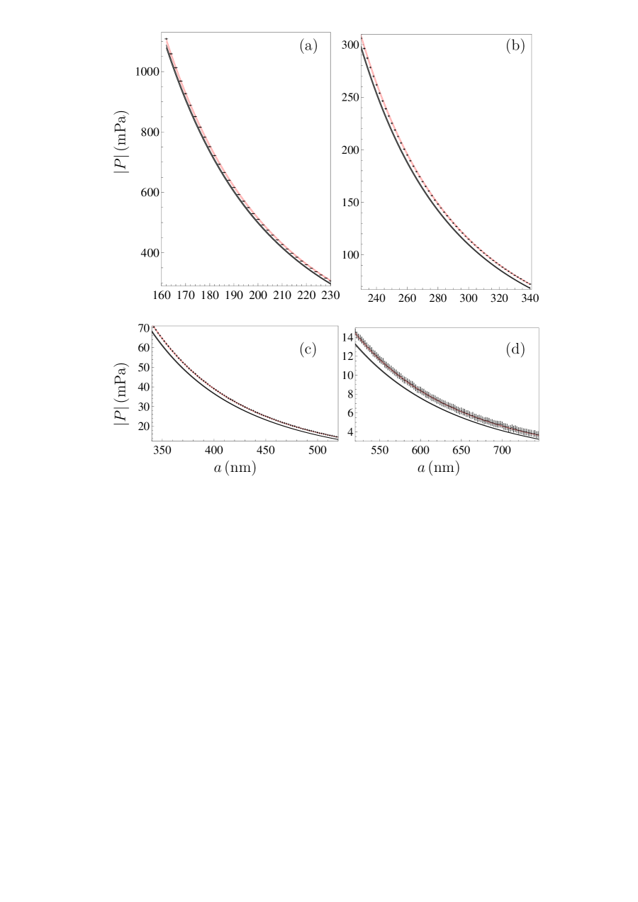
Figure 1: The magnitudes of the effective Casimir pressure between two Au-coated parallel plates computed using the spatially nonlocal response functions and the Drude model are shown as functions of separation by the upper (red) and lower (black) bands, respectively. The experimental data 27 are shown as crosses whose arms indicate the total errors determined at the 95% confidence level.

The computational results for the magnitude of the effective Casimir pressure are shown by the upper (red) theoretical bands in Figs. 1(a)–1(d) over four separation regions from 162.03 to 745.98 nm. The experimental data are shown as crosses. The horizontal and vertical arms of these crosses indicate the total measurement errors found at the 95% confidence level as a combination of systematic and random errors 27 . The lower (black) theoretical bands in Fig. 1 indicate the theoretical predictions of the Lifshitz theory obtained by Eqs. (2) and (3) using the standard local Drude response function (32). The width of each theoretical band is determined by the errors in all the above theoretical parameters used in computations.

As is seen in Fig. 1, the measurement data are in a very good agreement with theoretical predictions of the Lifshitz theory made using the spatially nonlocal response functions (8), (10) which take into account the dissipation properties of conduction electrons. Almost the same theoretical predictions in agreement with the measurement data were made by the Lifshitz theory using the plasma response function given by Eq. (32) with $\gamma_{n}=0$, i.e., with the relaxation properties of free electrons disregarded. The respective theoretical bands cannot be distinguished from the upper (red) bands shown in Fig. 1. As to the lower (black) theoretical bands in Fig. 1 computed using the Drude response function (32), they are excluded by the measurement data over the entire range of separations.

We are coming now to the recently performed experiment on measuring the differential Casimir force between an Au-coated sphere of $R=149.7~{}\mu$m radius and top and bottom of the Au-coated rectangular trenches 37 . As most of precise measurements of the Casimir interaction, this one was made at room temperature in high vacuum. Thanks to the differential character of this measurement, it has been made possible to obtain the meaningful data up to separation distances of a few micrometers using the same setup of a micromechanical torsional oscillator. Due to the sufficiently deep trenches used, the effectively measured Casimir force was that acting between a sphere and a plate which served as the trench top.

In the framework of the proximity force approximation, the Casimir force acting between a sphere and a plate is given by

$$F_{sp}(a,T)=2\pi R{\cal F}(a,T),$$ (34)

where the Casimir free energy in the configuration of two parallel plates is presented in Eq. (2). In Ref. 37 , the force $F_{sp}$ was computed both approximately using Eqs. (2), (3), and (34) and precisely on the basis of first principles of quantum electrodynamics at nonzero temperature using the scattering approach 84 ; 85 ; 86 ; 87 and the gradient expansion 88 ; 89 ; 90 ; 91 . It was shown 37 that all differences between the approximate and exact results are well below the measurement errors within the separation region from 0.2 to $8~{}\mu$m, irrespective of whether the Drude or plasma response function is used in computations.

The obtained theoretical results employing the plasma model given by Eq. (32) with $\gamma_{n}=0$ were found to be in a good agreement with the measurement data over the entire range of separations. The results computed similarly, but using the Drude model, were excluded by the data over the separation region from 0.2 to $4.8~{}\mu$m. In so doing the background electric force due to patch potentials was investigated with the help of Kelvin probe microscopy 92 and included in the total experimental error of the Casimir force determined at the 95% confidence level.

Here, we compute the Casimir force in the configuration of the experiment 37 by the first equality in Eq. (2) and Eq. (34) using the proposed spatially nonlocal dielectric functions (10). For the reflection coefficients with $l=0$, Eqs. (14), (15) and (20), (21) have been used, and for $l\geqslant 1$ numerical computations were performed by Eqs. (23) and (25) as described above with the following values of all parameters of Au 37 : $\hbar\omega_{p,{\rm Au}}=9.0~{}$eV, $\hbar\gamma_{\rm Au}=35.0~{}$meV, $v_{\rm F,Au}=1.78\times 10^{6}~{}$m/s. The obtained results were multiplied by a correction factor accounting for an inaccuracy of the proximity force approximation which was calculated in Ref. 37 .

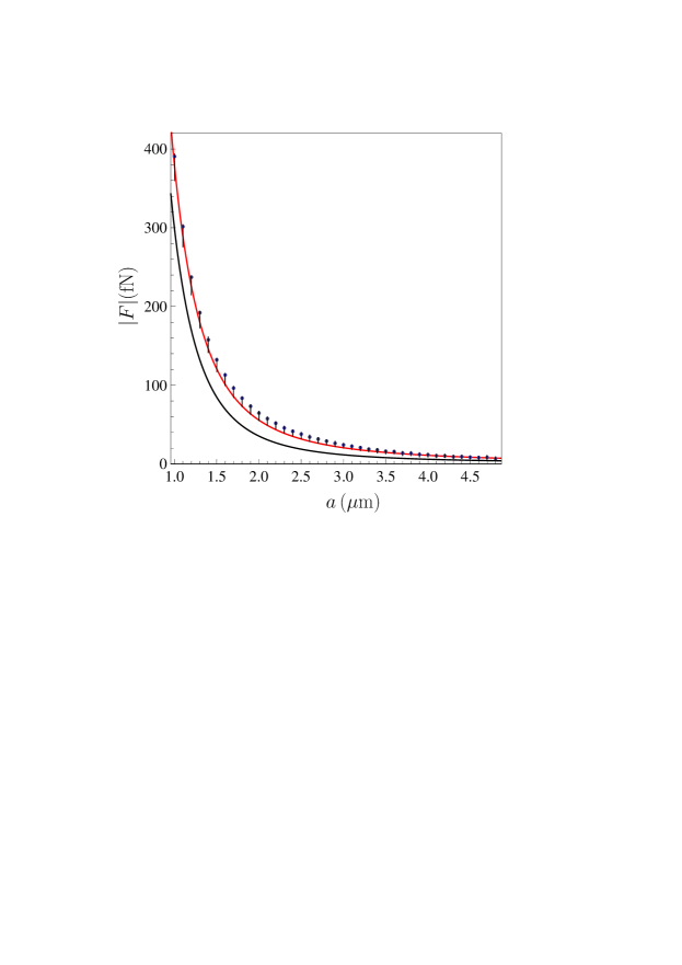
Figure 2: The magnitudes of the Casimir force between an Au-coated sphere and an Au-coated plate computed using the spatially nonlocal response functions and the Drude model are shown as functions of separation by the upper (red) and lower (black) bands, respectively. The experimental data 37 are shown as crosses whose arms indicate the total errors determined at the 95% confidence level.

The obtained computational results in the range of separations from 1 to $4.9~{}\mu$m are shown by the upper (red) band in Fig. 2. In the same figure, the lower (black) band is computed by Eqs. (2), (3) and (34) using the Drude response function (32). The measurement data are indicated as crosses. As is seen in Fig. 2, the upper and lower vertical arms of the crosses differ from one another. This is because the attractive electric force due to patch potentials is included as part of the error in measuring the Casimir force. According to Fig. 2, the theoretical predictions of the Lifshitz theory using the proposed nonlocal response functions (8), (10) are in agreement with the measurement data. Good agreement also holds over the ranges of separations from 0.2 to $1~{}\mu$m and from 4.8 to $8~{}\mu$m which are not shown in Fig. 2. The predictions of the same theory using the Drude model are excluded over the range of separations from 1 to $4.8~{}\mu$m (in Ref. 37 it is shown that they are also excluded in the measurement range from 0.2 to $1~{}\mu$m but here we are more interested in the region of large separations exceeding $1~{}\mu$m).

The Casimir forces computed by Eqs. (2), (3) and (34) using the plasma model given by Eq. (32) with $\gamma_{n}=0$ are almost the same as the ones computed above with the spatially nonlocal response functions. Thus, at separations of 1, 3, 5, and $7~{}\mu$m the pairs of force magnitudes (in fN) computed using the nonlocal response functions and the plasma model are (372.98, 374.62), (21.44, 21.67), (7.24, 7.30), and (3.69, 3.71), i.e., only 0.44%, 1.06%, 0.8%, and 0.54% relative differences, well below the respective experimental errors. Although these results are not experimentally distinguishable, that ones obtained using the nonlocal response functions should be considered as preferable as they are obtained with taken into account relaxation properties of conduction electrons.

V Measurements between nonmagnetic test bodies by means of an atomic force microscope

Another experimental setup for measuring the Casimir interaction is an atomic force microscope whose sharp tip is replaced with a sphere of sufficiently large radius 93 . Here, we compare the measurement data of three most precise experiments on measuring the gradient of the Casimir force between an Au-coated sphere and an Au-coated plate obtained by means of a dynamic atomic force microscope 29 ; 36 with theoretical predictions using the nonlocal dielectric functions (10). All measurements were performed in high vacuum at room temperature. In interpretation of all these experiments the same parameters of Au, i.e., the values of $\omega_{p,{\rm Au}}$, $\gamma_{\rm Au}$, and ${\varepsilon}_{c}^{(\rm Au)}$, have been used as already listed in Sec. IV when describing measurements of the differential Casimir force between a sphere and a plate with rectangular trenches.

We start with the experiment of Ref. 29 which employed the sphere of $R=41.3~{}\mu$m radius. The theoretical force gradients were computed using the Lifshitz theory and the proximity force approximation with taken into account correction for its inaccuracy 29

$$F_{sp}^{\prime}(a,T)=-2\pi RP(a,T)\left[1+\theta(a,T)\frac{a}{R}\right],$$ (35)

where the Casimir pressure $P$ is given by the second expression in Eq. (2) with the Fresnel reflection coefficients (3) and at separations below $1~{}\mu$m the coefficient $\theta$ is negative and does not exceed unity (see Refs. 88 ; 89 ; 90 and the more complete results for different dielectric functions in Refs. 87 ; 91 ). The effect of surface roughness was taken into account perturbatively and shown to be negligibly small.

According to the results of Ref. 29 , the theoretical predictions obtained using the Drude model (32) are excluded by the measurement data within the range of separations from 235 to 420 nm. The same data turned out to be in a good agreement with theoretical predictions found by using the plasma model which does not take into account the relaxation properties of free electrons, i.e., put $\gamma_{\rm Au}=0$. Thus, the results obtained earlier in Refs. 25 ; 26 ; 27 ; 28 by means a micromechanical torsional oscillator were confirmed independently by using quite different laboratory setup.

                          

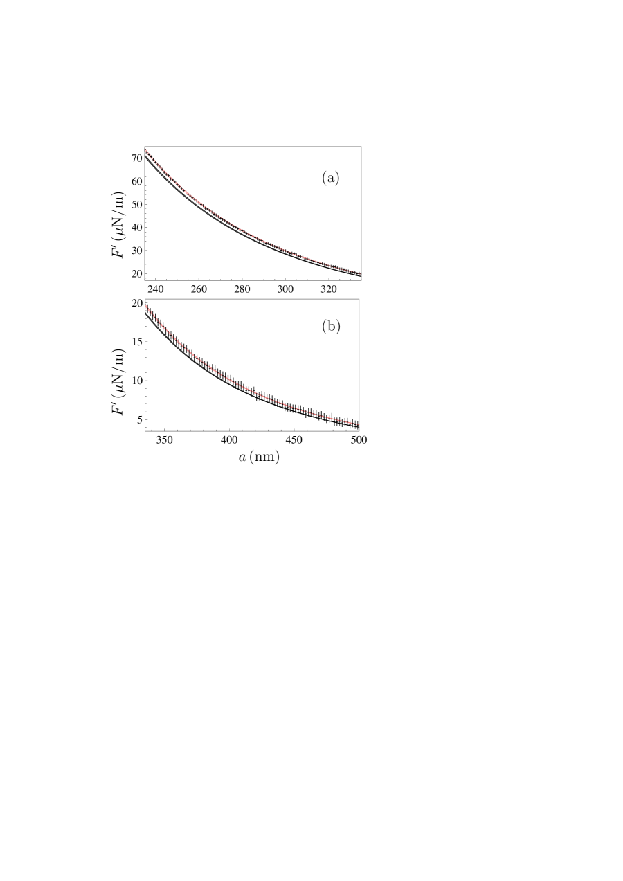
Figure 3: The gradients of the Casimir force between an Au-coated sphere and an Au-coated plate computed using the spatially nonlocal response functions and the Drude model are shown as functions of separation by the upper (red) and lower (black) bands, respectively. The experimental data 29 are shown as crosses whose arms indicate the total errors determined at the 67% confidence level.

We have computed the gradients of the Casimir force (35) in the experimental configuration of Ref. 29 using the spatially nonlocal response functions (10) and reflection coefficients (5) expressed via the surface impedances as described in Secs. III and IV. The same parameters of Au, as in Ref. 29 , have been used and $v_{n}^{\,\rm Tr,L}=v_{\rm Au}^{\,\rm Tr,L}=3v_{\rm F,Au}/2$ as indicated above. The computational results are shown by the upper (red) bands in Fig. 3 where the experimental data are presented as crosses whose arms indicate the total measurement errors determined at the 67% confidence level. The lower (black) bands in Fig. 3 reproduce the computational results of Ref. 29 obtained using the Drude model (32). In fact, our computational results using the nonlocal response functions are almost coinciding with the results of Ref. 29 using the dissipationless plasma model. In doing so, our results are in a good agreement with the measurement data over the entire range of separations which exclude the theoretical predictions using the Drude model over the separation range from 235 to 420 nm.

An upgraded setup employing the atomic force microscope with increased sensitivity of the cantilever through a decrease of its spring constant was used in Refs. 35 ; 36 in more precise measurements of the Casimir force gradients up to larger separation distances. The important property of an upgraded setup was an employment of the two-step cleaning procedure of the vacuum chamber and test body surfaces by means of UV light followed by Ar-ion bombardment. The radius of the sphere used was $R=43.47~{}\mu$m.

The comparison between experiment and theory in Ref. 36 was made as described above in this section using Eq. (35) and the dielectric response (32) with $\gamma_{\rm Au}\neq 0$ (the Drude model) and $\gamma_{\rm Au}=0$ (the plasma model). In the measurements with smaller oscillation amplitude of the cantilever equal to 10 nm, the theoretical predictions using the Drude model were excluded over the range of separations from 250 to 820 nm whereas those using the plasma model were found to be in agreement with the measurement data over the entire measurement range.

We have computed the gradient of the Casimir force in the experimental configuration of Refs. 35 ; 36 using the proposed dielectric functions (10) with the same parameters of Au, as in these references, and $v_{\rm Au}^{\,\rm Tr,L}=3v_{\rm F,Au}/2$ as above. The computational results are shown by the upper (red) bands in Fig. 4 as a function of separation. The measurement data with their errors determined at the 67% confidence level are shown as crosses. The theoretical predictions obtained using the Drude model 36 are presented by the lower (black) bands. As is seen in Fig. 4, our results, which take into account the dissipation of free electrons, are in agreement with the data over the entire separation region from 250 to 950 nm.

                          

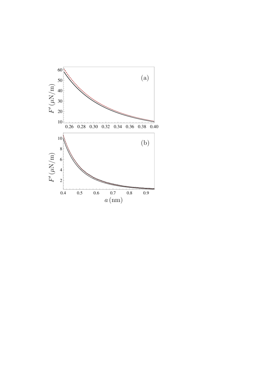
Figure 4: The gradients of the Casimir force between an Au-coated sphere and an Au-coated plate computed using the spatially nonlocal response functions and the Drude model are shown as functions of separation by the upper (red) and lower (black) bands, respectively. The experimental data 36 obtained with smaller oscillation amplitude of the cantilever are shown as crosses whose arms indicate the total errors determined at the 67% confidence level.

Another set of measurements was performed in Ref. 36 with a larger oscillation amplitude of cantilever equal to 20 nm. This made it possible to get the meaningful measurement data at larger separation distances and exclude theoretical predictions using the Drude model up to $1.1~{}\mu$m.

Our computational results for the gradient of the Casimir force obtained with the nonlocal dielectric functions (10) are presented by the upper (red) bands in Fig. 5 over the range of separations from 0.6 to $1.3~{}\mu$m of the data set in Ref. 36 measured with a larger oscillation amplitude. They are in a good agreement with the measurement data indicated as crosses. Our results accounting for the dissipation properties of free electrons are almost coinciding with those obtained in Ref. 36 using the dissipationless plasma model, but deviate significantly from those obtained by means of the Drude model. The latter are shown by the lower (black) bands.

One can conclude that the Lifshitz theory employing the proposed nonlocal dielectric permittivity is in equally good agreement with the measurement data of precise experiments performed by two different experimental groups by means of a micromechanical torsional oscillator and an atomic force microscope using test bodies made of a nonmagnetic metal.

                          

Figure 5: The gradients of the Casimir force between an Au-coated sphere and an Au-coated plate computed using the spatially nonlocal response functions and the Drude model are shown as functions of separation by the upper (red) and lower (black) bands, respectively. The experimental data 36 obtained with larger oscillation amplitude of the cantilever are shown as crosses whose arms indicate the total errors determined at the 67% confidence level.

VI Theory-experiment comparison with magnetic test bodies

The action of magnetic properties of the plate materials on the Casimir force has attracted considerable attention in the literature. Thus, although in Refs. 2 and 3 the Lifshitz formulas were derived for nonmagnetic test bodies, they were rewritten with account of magnetic properties in Ref. 94 . The Casimir force acting between an ideal metal plate and an infinitely permeable one was found in Ref. 95 . Thereafter the Casimir force between one magnetic and one nonmagnetic plates, as well as between two magnetic plates, was considered by many authors (see, e.g., Refs. 12 ; 75 ; 96 ; 97 ; 98 ). This problem attracted special attention in connection with the possibility of repulsive Casimir forces 42 .

As was emphasized in Ref. 99 , the magnetic properties of boundary plates make an impact on the Casimir free energy and pressure entirely through the zero-frequency terms of the Lifshitz formulas (2). This is caused by the fact that the frequency-dependent magnetic permeability becomes equal to unity at frequencies which are much smaller than the first Matsubara frequency at not too low temperature 100 ; 101 .

We begin with an experiment of Ref. 30 where the gradient of the Casimir force was measured between an Au-coated sphere of $R=64.1~{}\mu$m radius and a plate coated with a magnetic metal Ni by means of an atomic force microscope. Note that in measuring of the Casimir force using magnetic metals they are not magnetized and do not give rise to a gradient of any additional force of magnetic origin 32 . In Ref. 30 the theoretical force gradients were computed by Eq. (35) with the Fresnel reflection coefficients (3) and spatially local dielectric permittivities (32) with $\gamma_{\rm Au}\neq 0$ (the Drude model) and $\gamma_{\rm Au}=0$ (the plasma model) at room temperature. The following values of parameters for Au ($n=1$) and Ni ($n=2$) have been used: $\hbar\omega_{p,1}=\hbar\omega_{p,{\rm Au}}=9.0~{}$eV, $\hbar\gamma_{1}=\hbar\gamma_{\rm Au}=35.0~{}$meV 40 ; 41 ; 83 and $\mu_{1}(i\xi_{l})=\mu_{\rm Au}(i\xi_{l})=1$; $\hbar\omega_{p,2}=\hbar\omega_{p,{\rm Ni}}=4.89~{}$eV, $\hbar\gamma_{2}=\hbar\gamma_{\rm Ni}=43.6~{}$meV 83 ; 102 and $\mu_{2}(0)=\mu_{\rm Ni}(0)=110$, $\mu_{2}(i\xi_{l})=\mu_{\rm Ni}(i\xi_{l})=1$ for $l\geqslant 1$. The values of ${\varepsilon}_{c}^{(1)}(i\xi_{l})={\varepsilon}_{c}^{(\rm Au)}(i\xi_{l})$ and ${\varepsilon}_{c}^{(2)}(i\xi_{l})={\varepsilon}_{c}^{(\rm Ni)}(i\xi_{l})$ were obtained from the optical data of Au and Ni, respectively, as described in Refs. 29 ; 30 ; 32 ; 40 ; 41 .

According to the results of Ref. 30 , within the measurement range from 220 to 500 nm the theoretical predictions of the Lifshitz theory using the Drude and the plasma models are almost coinciding and are in a good agreement with the measurement data. (Note that at larger separations of a few micrometers the gradients of the Casimir force between a nonmagnetic-metal sphere and a magnetic-metal plate computed using the Drude and plasma models are different 99 .) The predictions obtained by means of the plasma model with magnetic properties of the Ni plate disregarded [$\mu_{\rm Ni}(i\xi_{l})=1$ for all $l\geqslant 0$] are excluded by the measurement data over the range of separations from 220 to 420 nm. If the Drude model is used in computations, the obtained results do not depend on whether the magnetic properties of Ni plate are included or omitted.

Here, we compute the gradient of the Casimir force in the experimental configuration of Ref. 30 using Eq. (35) and the spatially nonlocal dielectric permittivities (10). When computing the Casimir pressure, we have used the impedance reflection coefficients (5) for Au and Ni leading to Eqs. (14), (15) and (19), (20) for $l=0$ and Eqs. (23), (25) for $l\geqslant 1$. The same parameters for Au and Ni, as indicated above have been used and the Fermi velocity for Ni was found from Eq. (33) under an assumption of the spherical Fermi surface, $v_{\rm F,Ni}=1.31\times 10^{6}~{}$m/s (for Au we used $v_{\rm F,Au}=1.78\times 10^{6}~{}$m/s employed in Sec. IV and V). As in all previously considered experiments, the best agreement between the measurement data and theoretical predictions is reached for $v_{\rm Au}^{\rm Tr}=v_{\rm Au}^{\rm L}=3v_{\rm F,Au}/2$ and $v_{\rm Ni}^{\rm Tr}=v_{\rm Ni}^{\rm L}=3v_{\rm F,Ni}/2$.

                          

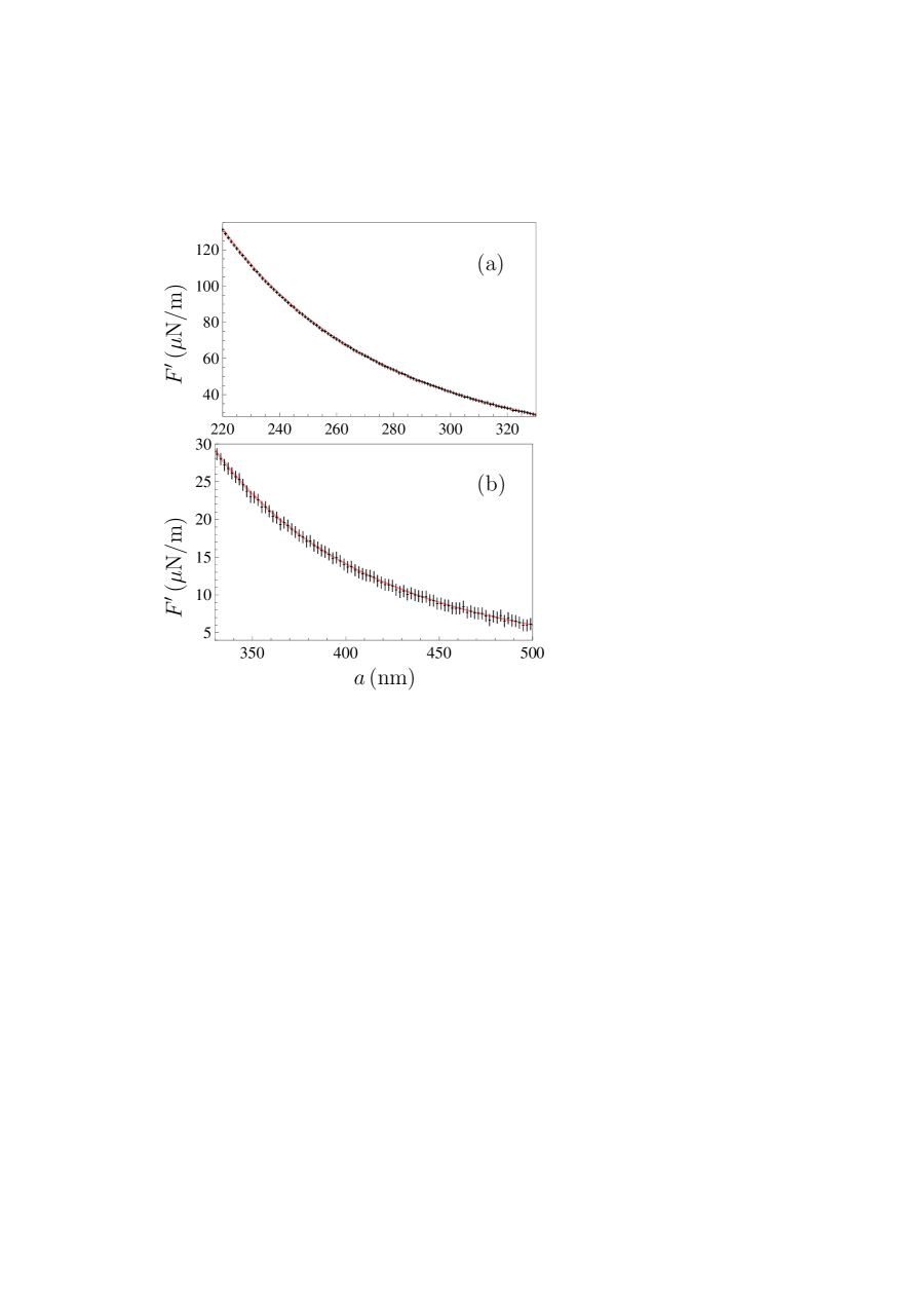
Figure 6: The gradients of the Casimir force between an Au-coated sphere and a Ni-coated plate computed using the spatially nonlocal response functions are shown by the solid (red) bands as a function of separation. The experimental data 30 are shown as crosses whose arms indicate the total errors determined at the 67% confidence level.

Computational results obtained using the spatially nonlocal dielectric permittivities (10) are shown by the solid (red) bands in Fig. 6 where the experimental data with their total errors determined at the 67% confidence level are presented as crosses. As is seen in Fig. 6, the theoretical predictions of the Lifshitz theory employing the proposed nonlocal dielectric functions are in a very good agreement with the measurement data over the entire range of experimental separations. For the configuration of Au-Ni test bodies in the range from 220 to 500 nm almost the same theoretical predictions in equally good agreement with the measurement data are obtained when the conduction electrons are described by the spatially local Drude or plasma model.

Next, we consider the experiment of Refs. 31 ; 32 on measuring the gradient of the Casimir force between a sphere of $R=61.71~{}\mu$m radius and a plate both coated with a magnetic metal Ni performed by means of an atomic force microscope. In these references computations of the force gradient using the standard Lifshitz theory were performed as in Sec. V but with the parameters $\omega_{p,1}=\omega_{p,2}=\omega_{p,{\rm Ni}}$, $\gamma_{1}=\gamma_{2}=\gamma_{\rm Ni}$, and ${\varepsilon}_{c}^{(1)}(i\xi_{l})={\varepsilon}_{c}^{(2)}(i\xi_{l})={\varepsilon}_{c}^{(\rm Ni)}(i\xi_{l})$ presented above. An important result found in Ref. 31 is that for two magnetic metals the gradients of the Casimir force calculated using the Drude model are larger than those found by means of the plasma model. This is different from the case of two Au plates (see Figs. 3–5). It was shown 31 ; 32 that the theoretical predictions obtained with the Drude model are excluded by the data over the separation region from 223 to 420 nm, whereas similar predictions made with the help of a plasma model are in a very good agreement with the measurement results. Similar to the case of test bodies coated with Au films, this result is puzzling because at low frequencies the relaxation properties of conduction electrons are well studied in many physical phenomena other than the Casimir effect.

                          

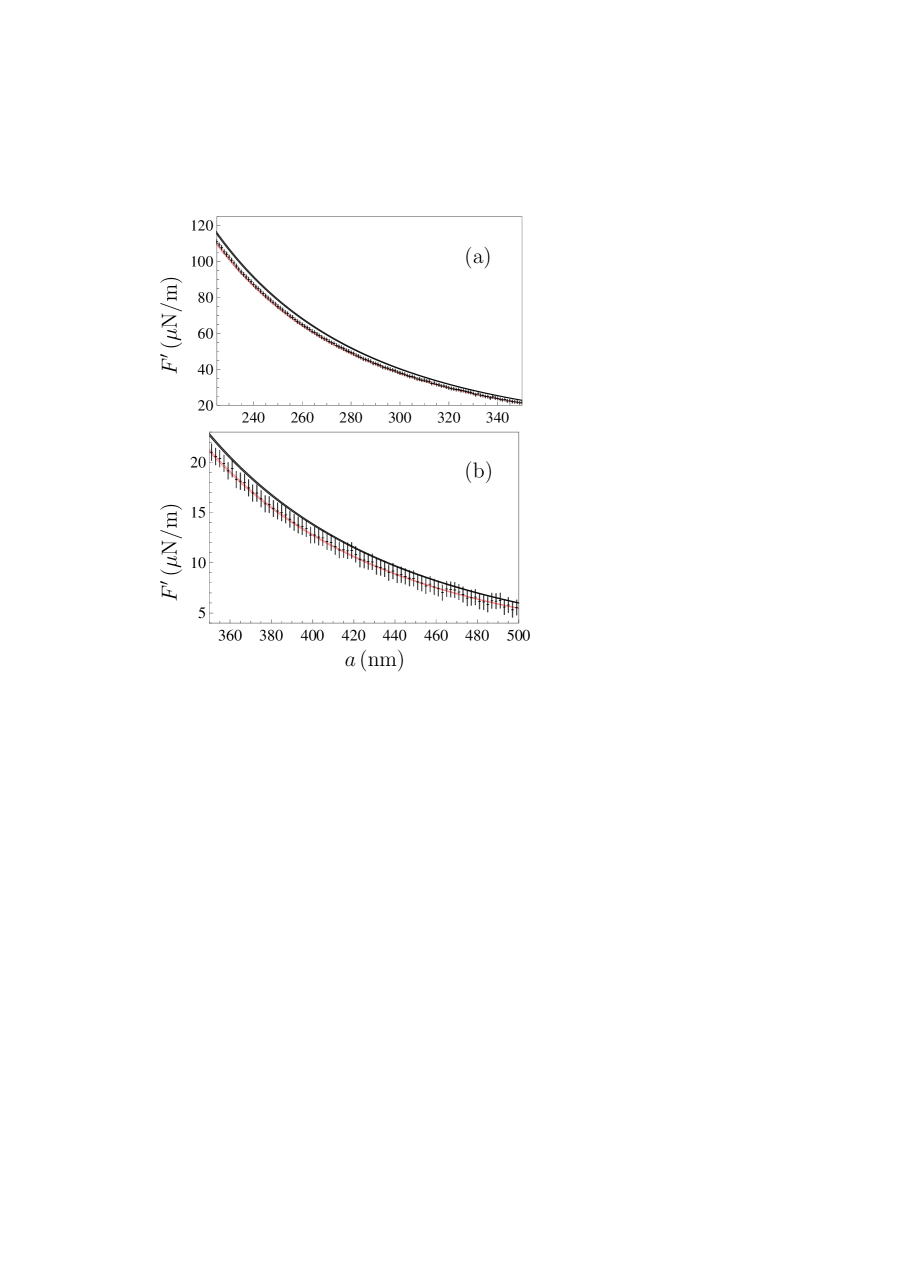
Figure 7: The gradients of the Casimir force between a Ni-coated sphere and a Ni-coated plate computed using the spatially nonlocal response functions and the Drude model are shown as functions of separation by the lower (red) and upper (black) bands, respectively. The experimental data 31 ; 32 are shown as crosses whose arms indicate the total errors determined at the 67% confidence level.

Here, we computed the gradient of the Casimir force between the Ni-coated surfaces of a sphere and a plate by Eq. (35). The Casimir pressure in this equation was found from the second line in Eq. (2), reflection coefficients (5), and impedance functions (7), as described above, using the spatially nonlocal dielectric permittivities (10) with the same parameters of Ni as above. The computational results are shown by the lower (red) bands in Fig. 7 as a function of separation. They are in a very good agreement with the measurement data indicated as crosses. As in all other experiments using an atomic force microscope, the total experimental errors are determined at the 67% confidence level. The upper (black) bands in Fig. 7 reproduce the results of Refs. 31 ; 32 computed by the Lifshitz formula and the spatially local Drude model (32). It is seen that these results are excluded by the measurement data over the separation region from 223 to 420 nm in accordance with the conclusion made in Refs. 31 ; 32 . The point is that at short separations up to a few hundred nanometers the force gradients computed using the local plasma model, which disregards the relaxation of free electrons, and the spatially nonlocal dielectric functions (10), which take relaxation into account, are almost coinciding. In this situation, a failure of the Drude model may be explained by an inadequate description of the dielectric response to electromagnetic waves off the mass shell.

VII Conclusions and discussion

In this paper, we have proposed the phenomenological spatially nonlocal dielectric functions which provide nearly the same response to electromagnetic waves on the mass shell, as does the standard Drude model, but respond differently to the off-the-mass-shell fields. Unlike the previously suggested response functions of this kind 71 ; 72 ; 73 , the permittivities presented here depend on all the three components of the wave vector which is a more general case in the approximation of specular reflection used.

As discussed in Sec. I, the problem of disagreement between theoretical predictions of the fundamental Lifshitz theory using the well-tested Drude model with the experimental data for metallic test bodies remains unresolved for almost 20 years. Many attempts of its resolution have been undertaken (including a consideration of the frequency-dependent relaxation parameter 103 , i.e., the so-called Gurzhi model), but the problem is as yet unresolved. Similar problem arises for dielectric materials 45 ; 104 . All this makes it warranted to consider some phenomenological approaches suggested by analogy with graphene which, due to its simplicity in comparison with metallic materials, allows the fundamental calculation of its spatially nonlocal dielectric response based on the first principles of quantum electrodynamics at nonzero temperature.

Using this line of reasoning, the surface impedances and reflection coefficients determined by the proposed nonlocal dielectric functions have been found in the approximation of specular reflection. This made it possible to calculate the effective Casimir pressure between two parallel metallic plates, the Casimir force between a sphere and a plate, and its gradient predicted by the suggested approach in configurations of several precise experiments performed during the last 15 years by two different experimental groups by means of micromechanical torsional oscillator and atomic force microscope. In doing so the experiments with both nonmagnetic and magnetic test bodies were considered.

It was shown that the suggested spatially nonlocal dielectric functions taking into account the dissipation properties of conduction electrons bring the Lifshitz theory to equally good agreement with the measurement data of all the performed experiments as does the plasma model which disregards the dissipation of conduction electrons. Good agreement with seven considered experiments, which were performed between both nonmagnetic and magnetic metallic surfaces (Au-Au, Au-Ni, and Ni-Ni), was reached with the velocity parameters common to the transverse and longitudinal permittivities ${v_{n}^{\rm Tr}}={v_{n}^{\,\rm L}}=v_{n}=3v_{{\rm F},n}/2$, where the Fermi velocities $v_{{\rm F},n}$ are determined in the approximation of a spherical Fermi surface. In doing so, the theoretical predictions are rather sensitive to the value of ${v_{n}^{\rm Tr}}$ but are almost independent on ${v_{n}^{\,\rm L}}$ in the region from 0 to $10v_{{\rm F},n}$. In the regions of experimental separations these predictions differ from the previously made experimentally consistent predictions using the dissipationless plasma models only in the limits of measurement errors.

The single precise experiment which was not compared with theoretical predictions of the suggested nonlocal approach to calculation of the Casimir force is the measurement of differential Casimir force between the Ni-Ni surfaces of a sphere and a plate performed by means of a micromechanical torsional oscillator 33 . Taking into account, however, that experiments by means of both an atomic force microscope and micromechanical torsional oscillator are in a good agreement with this calculation approach for Au surfaces, the results of Sec. VI for two magnetic surfaces can be safely extended to the experiment of Ref. 33 .

To conclude, the suggested spatially nonlocal dielectric functions include the dissipation of conduction electrons leading to only negligibly small deviations from the standard Drude dielectric response in the area of propagating waves on the mass shell, satisfy the Kramers-Kronig relations, and bring the theoretical predictions of the Lifshitz theory in agreement with the measurement data of all precise experiments on measuring the Casimir force. In the future it is desirable to provide some grounding in theory to these permittivities based, e.g., on the polarization tensor in (3+1)-dimensions 105 , or quantum field theoretical approach to correlation functions and Boltzmann kinetic theory 106 .

References

- (1) H. B. G. Casimir, On the attraction between two perfectly conducting bodies, Proc. Kon. Ned. Akad. Wet. B 51, 793 (1948).
- (2) E. M. Lifshitz, The theory of molecular attractive forces between solids, Zh. Eksp. Teor. Fiz. 29, 94 (1955) [Sov. Phys. JETP 2, 73 (1956)].
- (3) E. M. Lifshitz and L. P. Pitaevskii, Statistical Physics, Part II (Pergamon, Oxford, 1980).
- (4) N. G. Van Kampen, B. R. A. Nijboer, and K. Schram, On the macroscopic theory of Van der Waals forces, Phys. Lett. A 26, 307 (1968).
- (5) B. W. Ninham, V. A. Parsegian, and G. H. Weiss, On the macroscopic theory of temperature-dependent van der Waals forces, J. Stat. Phys. 2, 323 (1970).
- (6) K. Schram, On the macroscopic theory of retarded Van der Waals forces, Phys. Lett. A 43, 282 (1973).
- (7) D. Langbein, Theory of Van der Waals Attraction (Springer-Verlag, Berlin and Heidelberg, 2013).
- (8) T. Emig, R. L. Jaffe, M. Kardar, and A. Scardicchio, Casimir Interaction between a Plate and a Cylinder, Phys. Rev. Lett. 96, 080403 (2006).
- (9) M. Bordag, Casimir effect for a sphere and a cylinder in front of a plane and corrections to the proximity force theorem, Phys. Rev. D 73, 125018 (2006).
- (10) O. Kenneth and I. Klich, Casimir forces in a T-operator approach, Phys. Rev. B 78, 014103 (2008).
- (11) T. Emig, N. Graham, R. L. Jaffe, and M. Kardar, Casimir forces between compact objects: The scalar case, Phys. Rev. D 77, 025005 (2008).
- (12) S. J. Rahi, T. Emig, N. Graham, R. L. Jaffe, and M. Kardar, Scattering theory approach to electrodynamic Casimir forces, Phys. Rev. D 80, 085021 (2009).
- (13) M. Boström and Bo E. Sernelius, Thermal Effects on the Casimir Force in the 0.1–5 m Range, Phys. Rev. Lett. 84, 4757 (2000).
- (14) M. Bordag, B. Geyer, G. L. Klimchitskaya, and V. M. Mostepanenko, Casimir Force at Both Nonzero Temperature and Finite Conductivity, Phys. Rev. Lett. 85, 503 (2000).
- (15) V. B. Bezerra, G. L. Klimchitskaya, and V. M. Mostepanenko, Thermodynamic aspects of the Casimir force between real metals at nonzero temperature, Phys. Rev. A 65, 052113 (2002).
- (16) V. B. Bezerra, G. L. Klimchitskaya, and V. M. Mostepanenko, Correlation of energy and free energy for the thermal Casimir force between real metals, Phys. Rev. A 66, 062112 (2002).
- (17) V. B. Bezerra, G. L. Klimchitskaya, V. M. Mostepanenko, and C. Romero, Violation of the Nernst heat theorem in the theory of thermal Casimir force between Drude metals, Phys. Rev. A 69, 022119 (2004).
- (18) M. Bordag and I. Pirozhenko, Casimir entropy for a ball in front of a plane, Phys. Rev. D 82, 125016 (2010).
- (19) M. Bordag, Low Temperature Expansion in the Lifshitz Formula, Adv. Math. Phys. 2014, 981586 (2014).
- (20) G. L. Klimchitskaya and V. M. Mostepanenko, Low-temperature behavior of the Casimir free energy and entropy of metallic films, Phys. Rev. A 95, 012130 (2017).
- (21) G. L. Klimchitskaya and C. C. Korikov, Analytic results for the Casimir free energy between ferromagnetic metals, Phys. Rev. A 91, 032119 (2015).
- (22) S. Boström and Bo E. Sernelius, Entropy of the Casimir effect between real metal plates, Physica A 339, 53 (2004).
- (23) I. Brevik, J. B. Aarseth, J. S. Høye, and K. A. Milton, Temperature dependence of the Casimir effect, Phys. Rev. E 71, 056101 (2005).
- (24) J. S. Høye, I. Brevik, S. A. Ellingsen, and J. B. Aarseth, Analytical and numerical verification of the Nernst theorem for metals, Phys. Rev. E 75, 051127 (2007).
- (25) R. S. Decca, E. Fischbach, G. L. Klimchitskaya, D. E. Krause, D. López, and V. M. Mostepanenko, Improved tests of extra-dimensional physics and thermal quantum field theory from new Casimir force measurements, Phys. Rev. D 68, 116003 (2003).
- (26) R. S. Decca, D. López, E. Fischbach, G. L. Klimchitskaya, D. E. Krause, and V. M. Mostepanenko, Precise comparison of theory and new experiment for the Casimir force leads to stronger constraints on thermal quantum effects and long-range interactions, Ann. Phys. (NY) 318, 37 (2005).
- (27) R. S. Decca, D. López, E. Fischbach, G. L. Klimchitskaya, D. E. Krause, and V. M. Mostepanenko, Tests of new physics from precise measurements of the Casimir pressure between two gold-coated plates, Phys. Rev. D 75, 077101 (2007).
- (28) R. S. Decca, D. López, E. Fischbach, G. L. Klimchitskaya, D. E. Krause, and V. M. Mostepanenko, Novel constraints on light elementary particles and extra-dimensional physics from the Casimir effect, Eur. Phys. J. C 51, 963 (2007).
- (29) C.-C. Chang, A. A. Banishev, R. Castillo-Garza, G. L. Klimchitskaya, V. M. Mostepanenko, and U. Mohideen, Gradient of the Casimir force between Au surfaces of a sphere and a plate measured using an atomic force microscope in a frequency-shift technique, Phys. Rev. B 85, 165443 (2012).
- (30) A. A. Banishev, C.-C. Chang, G. L. Klimchitskaya, V. M. Mostepanenko, and U. Mohideen, Measurement of the gradient of the Casimir force between a nonmagnetic gold sphere and a magnetic nickel plate, Phys. Rev. B 85, 195422 (2012).
- (31) A. A. Banishev, G. L. Klimchitskaya, V. M. Mostepanenko, and U. Mohideen, Demonstration of the Casimir Force between Ferromagnetic Surfaces of a Ni-Coated Sphere and a Ni-Coated Plate, Phys. Rev. Lett. 110, 137401 (2013).
- (32) A. A. Banishev, G. L. Klimchitskaya, V. M. Mostepanenko, and U. Mohideen, Casimir interaction between two magnetic metals in comparison with nonmagbetic test bodies, Phys. Rev. B 88, 155410 (2013).
- (33) G. Bimonte, D. López, and R. S. Decca, Isoelectronic determination of the thermal Casimir force, Phys. Rev. B 93, 184434 (2016).
- (34) J. Xu, G. L. Klimchitskaya, V. M. Mostepanenko, and U. Mohideen, Reducing detrimental electrostatic effects in Casimir-force measurements and Casimir-force-based microdevices, Phys. Rev. A 97, 032501 (2018).
- (35) M. Liu, J. Xu, G. L. Klimchitskaya, V. M. Mostepanenko, and U. Mohideen, Examining the Casimir puzzle with an upgraded AFM-based technique and advanced surface cleaning, Phys. Rev. B 100, 081406(R) (2019).
- (36) M. Liu, J. Xu, G. L. Klimchitskaya, V. M. Mostepanenko, and U. Mohideen, Precision measurements of the gradient of the Casimir force between ultraclean metallic surfaces at larger separations, Phys. Rev. A 100, 052511 (2019).
- (37) G. Bimonte, B. Spreng, P. A. Maia Neto, G.-L. Ingold, G. L. Klimchitskaya, V. M. Mostepanenko, and R. S. Decca, Measurement of the Casimir Force between 0.2 and m: Experimental Procedures and Comparison with Theory, Universe 7, 93 (2021).
- (38) A. O. Sushkov, W. J. Kim, D. A. R. Dalvit, and S. K. Lamoreaux, Observation of the thermal Casimir force, Nat. Phys. 7, 230 (2011).
- (39) V. B. Bezerra, G. L. Klimchitskaya, U. Mohideen, V. M. Mostepanenko, and C. Romero, Impact of surface imperfections on the Casimir force for lenses of centimeter-size curvature radii, Phys. Rev. B 83, 075417 (2011).
- (40) G. L. Klimchitskaya, U. Mohideen, and V. M. Mostepanenko, The Casimir force between real materials: Experiment and theory, Rev. Mod. Phys. 81, 1827 (2009).
- (41) M. Bordag, G. L. Klimchitskaya, U. Mohideen, and V. M. Mostepanenko, Advances in the Casimir Effect (Oxford University Press, Oxford, 2015).
- (42) L. M. Woods, D. A. R. Dalvit, A. Tkatchenko, P. Rodriguez-Lopez, A. W. Rodriguez, and R. Podgornik, Materials perspective on Casimir and van der Waals interactions, Rev. Mod. Phys. 88, 045003 (2016).
- (43) K. A. Milton, Y. Li, P. Kalauni, P. Parashar, R. Guérout, G.-L. Ingold, A. Lambrecht, and S. Reynaud, Negative Entropies in Casimir and Casimir-Polder Interactions, Fortschr. d. Phys. 65, 1600047 (2017).
- (44) G. Bimonte, T. Emig, M. Kardar, and M. Krüger, Nonequilibrium Fluctuational Quantum Electrodynamics: Heat Radiation, Heat Transfer, and Force, Ann. Rev. Condens. Matter Phys. 8, 119 (2017).
- (45) V. M. Mostepanenko, Casimir Puzzle and Conundrum: Discovery and Search for Resolution, Universe 7, 84 (2021).
- (46) A. H. Castro Neto, F. Guinea, N. M. R. Peres, K. S. Novoselov, and A. K. Geim, The electronic properties of graphene, Rev. Mod. Phys. 81, 109 (2009).
- (47) M. I. Katsnelson, The Physics of Graphene (Cambridge University Press, Cambridge, 2020).
- (48) M. Bordag, I. V. Fialkovsky, D. M. Gitman, and D. V. Vassilevich, Casimir interaction between a perfect conductor and graphene described by the Dirac model, Phys. Rev. B 80, 245406 (2009).
- (49) I. V. Fialkovsky, V. N. Marachevsky, and D. V. Vassilevich, Finite-temperature Casimir effect for graphene, Phys. Rev. B 84, 035446 (2011).
- (50) M. Bordag, G. L. Klimchitskaya, V. M. Mostepanenko, and V. M. Petrov, Quantum field theoretical description for the reflectivity of graphene, Phys. Rev. D 91, 045037 (2015); 93, 089907(E) (2016).
- (51) M. Bordag, I. Fialkovskiy, and D. Vassilevich, Enhanced Casimir effect for doped graphene, Phys. Rev. B 93, 075414 (2016); 95, 119905(E) (2017).
- (52) A. A. Banishev, H. Wen, J. Xu, R. K. Kawakami, G. L. Klimchitskaya, V. M. Mostepanenko, and U. Mohideen, Measuring the Casimir force gradient from graphene on a SiO2 substrate, Phys. Rev. B 87, 205433 (2013).
- (53) G. L. Klimchitskaya, U. Mohideen, and V. M. Mostepanenko, Theory of the Casimir interaction for graphene-coated substrates using the polarization tensor and comparison with experiment, Phys. Rev. B 89, 115419 (2014).
- (54) M. Liu, Y. Zhang, G. L. Klimchitskaya, V. M. Mostepanenko, and U. Mohideen, Demonstration of an Unusual Thermal Effect in the Casimir Force from Graphene, Phys. Rev. Lett. 126, 206802 (2021).
- (55) M. Liu, Y. Zhang, G. L. Klimchitskaya, V. M. Mostepanenko, and U. Mohideen, Experimental and theoretical investigation of the thermal effect in the Casimir interaction from graphene, Phys. Rev. B 104, 085436 (2021).
- (56) G. L. Klimchitskaya and V. M. Mostepanenko, Low-temperature behavior of the Casimir-Polder free energy and entropy for an atom interacting with graphene, Phys. Rev. A 98, 032506 (2018).
- (57) G. L. Klimchitskaya and V. M. Mostepanenko, Nernst heat theorem for an atom interacting with graphene: Dirac model with nonzero energy gap and chemical potential, Phys. Rev. D 101, 116003 (2020).
- (58) G. L. Klimchitskaya and V. M. Mostepanenko, Quantum field theoretical description of the Casimir effect between two real graphene sheets and thermodynamics, Phys. Rev. D 102, 016006 (2020).
- (59) G. L. Klimchitskaya and V. M. Mostepanenko, Casimir and Casimir-Polder Forces in Graphene Systems: Quantum Field Theoretical Description and Thermodynamics, Universe 6, 150 (2020).
- (60) N. Khusnutdinov and N. Emelianova, The Low-Temperature Expansion of the Casimir-Polder Free Energy of an Atom with Graphene, Universe 7, 70 (2021).
- (61) J. Lindhard, On the properties of a gas of charged particles, Dan. Mat. Fys. Medd. 28, 1 (1954).
- (62) V. P. Silin and E. P. Fetisov, Electromagnetic properties of a relativistic plasma, III, Zh. Eksp. Teor. Fiz. 41, 159 (1961) [Sov. Phys. JETP 14, 115 (1962)].
- (63) K. L. Kliewer and R. Fuchs, Anomalous Skin Effect for Specular Electron Scattering and Optical Experiments at Non-Normal Angles of Incidence, Phys. Rev. 172, 607 (1968).
- (64) N. D. Mermin, Lindhard Dielectric Function in the Relaxation Time Approximation, Phys. Rev. B 1, 2362 (1970).
- (65) J.-N. Chazalviel, Coulomb Screening of Mobile Charges: Applications to Material Science, Chemistry and Biology (Birkhauser, Boston, 1999).
- (66) M. Dressel and G. Grüner, Electrodynamics of Solids: Optical Properties of Electrons in Metals (Cambridge University Press, Cambridge, 2003).
- (67) H. R. Haakh and C. Henkel, Magnetic near fields as a probe of charge transport in spatially dispersive conductors, Eur. Phys. J. B 85, 46 (2012).
- (68) E. I. Kats, Influence of nonlocality effects on van der Waals interaction, Zh. Eksp. Teor. Fiz. 73, 212 (1977) [Sov. Phys. JETP 46, 109 (1977)].
- (69) R. Esquivel, C. Villarreal, and W. L. Mochán, Exact surface impedance formulation of the Casimir force: Application to spatially dispersive metals, Phys. Rev. A 68, 052103 (2003); 71, 029904(E) (2005).
- (70) R. Esquivel and V. B. Svetovoy, Correction to the Casimir force due to the anomalous skin effect, Phys. Rev. A 69, 062102 (2004).
- (71) V. B. Svetovoy and R. Esquivel, Nonlocal impedances and the Casimir entropy at low temperatures, Phys. Rev. E 72, 036113 (2005).
- (72) Bo E. Sernelius, Effects of spatial dispersion on electromagnetic surface modes and on modes associated with a gap between two half spaces, Phys. Rev. B 71, 235114 (2005).
- (73) G. L. Klimchitskaya, V. M. Mostepanenko, An alternative response to the off-shell quantum fluctuations: a step forward in resolution of the Casimir puzzle, Eur. Phys. J. C 80, 900 (2020).
- (74) G. L. Klimchitskaya and V. M. Mostepanenko, Casimir entropy and nonlocal response functions to the off-shell quantum fluctuations, Phys. Rev. D 103, 096007 (2021).
- (75) M. Hannemann, G. Wegner, and C. Henkel, No-Slip Boundary Conditions for Electron Hydrodynamics and the Thermal Casimir Pressure, Universe 7, 108 (2021).
- (76) G. L. Klimchitskaya and V. M. Mostepanenko, Casimir effect for magnetic media: Spatially nonlocal response to the off-shell quantum fluctuations, Phys. Rev. D 104, 085001 (2021).
- (77) L. D. Landau, E. M. Lifshitz, and L. P. Pitaevskii, Electrodynamics of Continuous Media (Pergamon, Oxford, 1984).
- (78) Yu. S. Barash and V. L. Ginzburg, Electromagnetic fluctuations in a substance and molecular (van der Waals) interbody forces, Usp. Fiz. Nauk 116, 5 (1975) [Sov. Phys. Usp. 18, 305 (1975)].
- (79) G. L. Klimchitskaya and V. M. Mostepanenko, Comment on “Effects of spatial dispersion on electromagnetic surface modes associated with a gap between two half spaces”, Phys. Rev. B 75, 036101 (2007).
- (80) V. M. Agranovich and V. L. Ginzburg, Crystal Optics with Spatial Dispersion and Excitons (Springer, Berlin, 1984).
- (81) G. W. Ford and W. H. Weber, Electromagnetic interactions of molecules with metal surfaces, Phys. Rep. 113, 195 (1984).
- (82) J. T. Foley and A. J. Devaney, Electrodynamics of nonlocal media, Phys. Rev. B 12, 3104 (1975).
- (83) V. A. Parsegian, Van der Waals Forces: A Handbook for Biologists, Chemists, Engineers, and Physicists (Cambridge University Press, Cambridge, 2005).
- (84) A. P. Prudnikov, Yu. A. Brychkov, and O. I. Marichev, Integrals and Series. Vol. 1. Elementary Functions (Gordon and Breach, New York, 1986).
- (85) M. Bordag, G. L. Klimchitskaya, and V. M. Mostepanenko, The Casimir force between plates with small deviations from plane-parallel geometry, Int. J. Mod. Phys. A 10, 2661 (1995).
- (86) P. J. van Zwol, G. Palasantzas, and J. Th. M. De Hosson, Influence of random roughness on the Casimir force at small separations, Phys. Rev. B 77, 075412 (2008).
- (87) W. Broer, G. Palasantzas, J. Knoester, and V. B. Svetovoy, Roughness correction to the Casimir force at short separations: Contact distance and extreme value statistics, Phys. Rev. B 85, 155410 (2012).
- (88) Handbook of Optical Constants of Solids, ed. E. D. Palik (Academic, New York, 1985).
- (89) B. Spreng, M. Hartmann, V. Henning, P. A. Maia Neto, and G.-L. Ingold, Proximity force approximation and specular reflection: Application of the WKB limit of Mie scattering to the Casimir effect, Phys. Rev. A 97, 062504 (2018).
- (90) V. Henning, B. Spreng, M. Hartmann, G.-L. Ingold, and P. A. Maia Neto, Role of diffraction in the Casimir effect beyond the proximity force approximation, J. Opt. Soc. Am. B 36, C77 (2019).
- (91) B. Spreng, P. A. Maia Neto, and G.-L. Ingold, Plane-wave approach to the exact van der Waals interaction between colloid particles, J. Chem. Phys. 153, 024115 (2020).
- (92) M. Hartmann, G.-L. Ingold, and P. A. Maia Neto, Plasma versus Drude Modeling of the Casimir Force: Beyond the Proximity Force Approximation, Phys. Rev. Lett. 119, 043901 (2017).
- (93) C. D. Fosco, F. C. Lombardo, and F. D. Mazzitelli, Proximity force approximation for the Casimir energy as a derivative expansion, Phys. Rev. D 84, 105031 (2011).
- (94) G. Bimonte, T. Emig, and M. Kardar, Material dependence of Casimir force: gradient expansion beyond proximity, Appl. Phys. Lett. 100, 074110 (2012).
- (95) G. Bimonte, T. Emig, R. L. Jaffe, and M. Kardar, Casimir forces beyond the proximity force approximation, Europhys. Lett. 97, 50001 (2012).
- (96) G. Bimonte, Going beyond PFA: A precise formula for the sphere-plate Casimir force, Europhys. Lett. 118, 20002 (2017).
- (97) R. O. Behunin, D. A. R. Dalvit, R. S. Decca, C. Genet, I. W. Jung, A. Lambrecht, A. Liscio, D. López, S. Reynaud, G. Schnoering, G. Voisin, and Y. Zeng, Kelvin probe force microscopy of metallic surfaces used in Casimir force measurements, Phys. Rev. A 90, 062115 (2014).
- (98) U. Mohideen and A. Roy, Precision Measurement of the Casimir Force from 0.1 to m, Phys. Rev. Lett. 81, 4549 (1998).
- (99) P. Richmond and B. W. Ninham, A note on the extension of the Lifshitz theory of van der Waals forces to magnetic media, J. Phys. C: Solid St. Phys. 4, 1988 (1971).
- (100) T. H. Boyer, Van der Waals forces and zero-point energy for dielectric and permeable materials, Phys. Rev. A 9, 2078 (1974).
- (101) O. Kenneth, I. Klich, A. Mann, and M. Revzen, Repulsive Casimir Forces, Phys. Rev. Lett. 89, 033001 (2002).
- (102) D. Iannuzzi and F. Capasso, Comment on “Repulsive Casimir Forces”, Phys. Rev. Lett. 91, 029101 (2003).
- (103) M. S. Tomaš, Casimir force between dispersive magnetodielectrics, Phys. Lett. A 342, 381 (2005).
- (104) B. Geyer, G. L. Klimchitskaya, and V. M. Mostepanenko, Thermal Casimir interaction between two magnetodielectric plates, Phys. Rev. B 81, 104101 (2010).
- (105) A. H. Morrish, The Physical Principles of Magnetism (J. Wiley, New York, 1965).
- (106) S. V. Vonsovskii, Magnetism (J. Wiley, New York, 1974).
- (107) M. A. Ordal, R. J. Bell, R. W. Alexander, L. L. Long, and M. R. Querry, Optical properties of fourteen metals in the infrared and far infrared: Al, Co, Cu, Au, Fe, Pb, Mo, Ni, Pd, Pt, Ag, Ti, V, and W, Appl. Optics 24, 4493 (1985).
- (108) G. L. Klimchitskaya, V. M. Mostepanenko, Kailiang Yu, and L. M. Woods, Casimir force, causality, and the Gurzhi model, Phys. Rev. B 101, 075418 (2020).
- (109) G. L. Klimchitskaya and V. M. Mostepanenko, Conductivity of dielectric and thermal atom-wall interaction. J. Phys. A: Math. Theor. 41, 312002 (2008).
- (110) M. Bordag, I. V. Fialkovsky, N. Khusnutdinov, and D. V. Vassilevich, Bulk contributions to Casimir interaction of Dirac materials, Phys. Rev. B 104, 195431 (2021).
- (111) A. Altland and B. D. Simons, Condensed Matter Field Theory (Cambridge University Press, Cambridge, 2010).