Compensating trajectory bias for unsupervised patient stratification using adversarial recurrent neural networks

Abstract

Electronic health records (EHRs) are an important source of information which can be used in patient stratification to discover novel disease phenotypes. However, they can be challenging to work with as data is often sparse and irregularly sampled. One approach to solve these limitations is learning dense embeddings that represent individual patient trajectories using a recurrent neural network autoencoder (RNN-AE). This process can be susceptible to unwanted data biases. We show that patient embeddings and clusters using previously proposed RNN-AE models might be impacted by a trajectory bias, meaning that results are dominated by the amount of data contained in each patients trajectory, instead of clinically relevant details. We investigate this bias on 2 datasets (from different hospitals) and 2 disease areas as well as using different parts of the patient trajectory. Our results using 2 previously published baseline methods indicate a particularly strong bias in case of an event-to-end trajectory. We present a method that can overcome this issue using an adversarial training scheme on top of a RNN-AE. Our results show that our approach can reduce the trajectory bias in all cases.

Adversarial Training, Electronic Health Records, Patient Stratification, Recurrent Neural Networks, Unsupervised Clustering

1 Introduction

In recent years, the availability of EHR data has increased dramatically. Such data contain the medical history of patients across multiple years, with information ranging from primary and secondary diagnosis codes and performed procedures to laboratory values and prescribed medications. We refer to the sequence of clinical observations of a patient as patient trajectory. Despite being a rich source of information, working with longitudinal real world EHR data is challenging. Typically EHRs consist of mixed data types (e.g. binary diagnoses codes and continuous laboratory values) and are highly irregularly sampled, sparse, and noisy.

Alongside clinical objectives, EHR data can be used to identify novel patient phenotypes to support the drug development process as well as validation within clinical trials [1]. The aim of patient stratification is to identify clinically meaningful groups of patients which share either similar characteristics along their patient trajectory (e.g. having similar comorbidities or medications prescribed) or clinical outcomes (e.g. mortality or probability of re-hospitalization) [2]. We refer to these two approaches as unsupervised and outcome based patient stratification, respectively.

In the case of unsupervised patient stratification, the general approach consists of two main steps: first, learning a dense patient representation, an embedding, of the original patient trajectory, and, second, performing a clustering of patients in the embedded space to identify novel subgroups. Learning a suitable embedding to represent patients medical history is non-trivial due to the longitudinal and noisy nature of EHR data, the fact that the data contains mixed data types, and the non linear relationship between the covariates.

This paper focuses on learning clinically meaningful representations from a large collection of EHR by compensating the trajectory bias (defined below) using an RNN-AE approach.

When using traditional RNN-AE approaches the learned embeddings as well as the identified patient clusters are often strongly determined by how much data is available across the individual trajectory of the patient. We refer to this as the trajectory bias. Even though this information might be an indicator of how healthy a patient is, i.e. the less data is available, the healthier the patient tends to be in many settings. However, the different amount of available data could also be due to the fact, for example, that the patient relocated and was treated in a different facility. Other reasons might be due to different ways of working across wards in a hospital; e.g. maybe not all data are recorded electronically, or due to the general IT infrastructure; e.g., data might get lost when being migrated across platforms. For these reasons, being able to represent and cluster patient trajectories in ways that are not overly sensitive to variations in the length of trajectory is desirable. There is a need to develop methods where the role of the amount of data within a patient trajectory is reduced and instead shift the focus towards other differentiating features in the data while increasing the robustness against missing information.

Furthermore, the effect of the trajectory bias becomes exacerbated if only specific parts of a patient trajectory are investigated. This is illustrated in Figure 1. Often, EHR datasets cover a specific time range, e.g. 2014-2019. If, for example, the objective is to stratify heart failure (HF) patients based on their trajectory/data before the first acute HF event, the trajectory lengths are very different as the event could occur in 2015 as for patient A and in 2018-19 for patient B and C. Assuming that data for patient B is available from 2014, it is less likely that patients A and B would be clustered together due to the different trajectory length even if they have similar clinical observations. We present a novel adversarial RNN-AE approach to reduce this trajectory bias within the embedding space, such that resulting clusters are more dependent on medical information rather than on the amount of data present within a time-series.

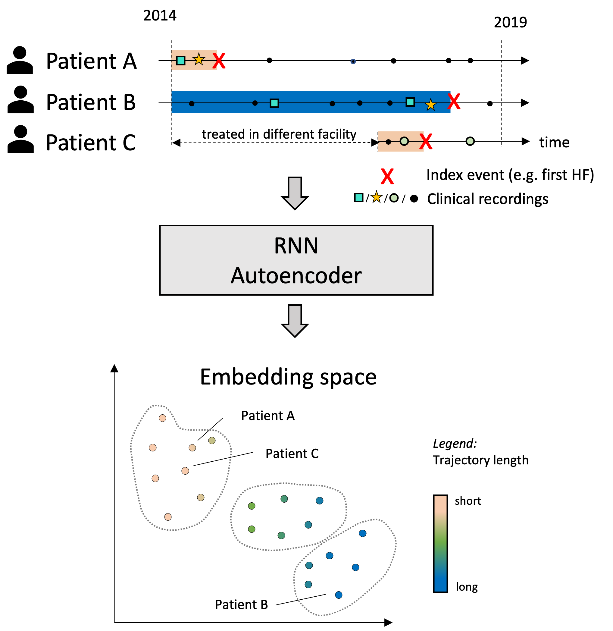
Figure 1: Illustration of trajectory bias. In this example, EHR data were obtained between 2014-19. Objective is to stratify patients based on data available before a given index event such as the first acute HF episode. Due to different amounts of data, patient A and B are more likely to be mapped to different clusters in the embedding space even if they share similar clinical observations. Dotted lines indicate potential result of a clustering algorithm. The colour of the trajectories of patients A, B and C indicates their trajectory length according to the legend at the bottom of the figure.

Our approach is evaluated over its ability to reduce trajectory bias across two cardiovascular EHR datasets from different hospitals which includes diagnoses, procedures, medication and laboratory values and a total of $N=623,364$ patients combined.

2 Literature

In recent years, an increasing amount of machine learning (and in particular deep learning)-based approaches have been investigated to identify novel patient phenotypes [2]. The general approach can be grouped into two steps: first, learning a dense patient embedding of the noisy, irregular sampled raw data, and, second, performing a cluster analysis on the embedded data [3, 4]. One solution is to use a recurrent neural network (RNN), which has been widely used in the context of supervised prediction tasks such as disease progression [5] or more recently in the context of supervised patient stratification [6].

Few studies have focused on learning a meaningful embedding for unsupervised phenotyping, which can be achieved using an autoencoder (AE) approach. Baytas and colleagues proposed to use a time-aware LSTM (tLSTM) AE network [3]. By explicitly including the time difference between admissions, they showed that they can learn a superior embedding compared to a simple long short-term memory (LSTM) using fixed time windows and imputation of missing information. Yin and colleagues suggested a different approach by using a bi-directional LSTM with an attention mechanism to focus on the important time windows [4]. This study is one of few which included continuous laboratory values in the analysis, which were imputed if missing or normalized to mean of zero and standard deviation of one. On the contrary the vast majority of publications only consider binary data [3, 7, 8, 9, 10, 11].

To the best of our knowledge, all published unsupervised patient stratification applied to real world EHR data focused on the analysis on all available data [3, 4]. Stratification of sections of a patient trajectory was not performed. However, analysis to answer questions such as “Are there specific subphenotypes which can be identified using data before the index event, e.g. first occurrence of a heart failure episode? ” are highly relevant for example, for early stage drug development or to optimize inclusion and exclusion criteria for clinical trials.

There are a number of papers in the literature that highlight the potential issues of trajectory bias. One paper discusses the general issue of auxiliary objective function deviating from the desired target task during embedding learning and refer to this problem as objective function mismatch (OFM) [12]. Our described problem of trajectory bias is an example of OFM where the auxiliary objective function, minimization of the AE reconstruction loss, does not match the primary objective, clustering. The information of the trajectory length is essential in achieving a small reconstruction error, but can lead to trajectory length being the dominating factor in the clustering results. While there are no examples in the literature that highlight this problem in EHR data, there are examples from other domains that utilise time-series data such as speech recognition. Trosten and colleagues carried out clustering on speech recordings of variable length and found that using sub-optimal embedding representations led to the length of a given speech sequence influencing it’s relative position in the embedding space [13]. Similarly, Lenco and colleagues demonstrated that data length can dominate clustering methods when used in speech and activity recognition datasets with variable input data length [14].

3 Methods

3.1 Dataset, cohorts and patient trajectories

Dataset. The dataset used in the present study consists of two cardiovascular patient cohorts provided by Oxford University Hospital (OUH) and Chelsea and Westminster Hospital (ChelWest), to each of which we refer as the wider cohort. Patients were included in this cohort based on the presence of any cardiovascular specific diagnosis, procedure or medication code throughout their patient history. The OUH wider cohort contains a total of $493,512$ patients, with records spanning from August 2014 to March 2020, and the ChelWest wider cohort a total of of $129,852$ patients, with records spanning from February 2014 to March 2020. The EHR data contains 4 separate types of clinical features: diagnosis codes (ICD-10 codes), procedure codes (OPCS-4 codes), medication codes (BNF codes), and laboratory values. Diagnosis codes could either appear in the data as a primary diagnosis (indicating the primary reason for the hospital admission) or secondary diagnosis (further present comorbidities). While the majority of these are binary or categorical features, laboratory values are continuous. In addition to this, administrative information, such as start date of admission, discharge date and admission type, were present.

Disease specific cohorts and patient trajectories. To investigate specific patient trajectories, we defined smaller cohorts with an index event, as shown in Figure 1. In this analysis, we defined the cohorts based on two diseases: acute HF or stroke. The smaller cohorts are a subset of the wider cohort for each trust, for whom the first instance of the diseases could be detected. This event was our index event. The inclusion and exclusion criteria for the first acute HF or stroke event are detailed in appendix 8.

In principle there can be 5 different trajectories investigated relative to a single index event:

• Before-event (BeE): the trajectory consists of all data available before the index event,

• Start-to-event (S2E): the trajectory consists of all data available before and at the index event (as sketched in Figure 1),

• Event-to-end (E2E): the trajectory consists of all data available at and after the index event,

• After-event (AfE): the trajectory consists of all data available after the index event, and

• ALL: considering the complete available data of the patient trajectory independently of the index event (maximum from 2014-2019).

Each of these trajectories can be relevant to answer different clinical questions. For instance, phenotyping of AfE and E2E trajectories could reveal groups of patients with an unmet medical need indicated by a lower survival rate or be used to model disease progression. In contrast, phenotypes based on data of a BeE or S2E trajectory can be used to support clinical trials if e.g. the index event aligns with the point of recruitment. As this study focuses on the impact of the trajectory bias from a methodological point of view, this paper only includes results of the E2E, AfE, and ALL trajectory. Similar effects were found using BeE and S2E trajectories.

Table II and Table III in appendix 7 provide a brief statistical overview of the considered cohorts and trajectories.

Data preprocessing. There is the risk of implicitly encoding the number windows with data when training the autoencoder using sequences of different lengths. Therefore, we decide to use equal length sequences for all patients. Each trajectory of a patient $j$ was divided into non overlapping time windows $x_{j,i}$ of 90 days, with $i$ being the time index.

As the data spanned more than five years, this resulted in up to $i_{max}=22$ windows per patient. Features with an occurrence of $<1\,\%$ within the wider cohort or the smaller cohorts were removed.

Features were extracted per time window if data was present. Time windows with no data of any type were filled with an empty vector consisting in zeros for the binary features, and -0.1 for the normalized continuous features.

The binary features (primary and secondary diagnosis, procedures and medication codes) were included using multi-hot encoding. Even though continuous laboratory values contain clinically relevant information, the integration of these in an unsupervised RNN-AE model and combination with further binary data is challenging, as the data need to be normalized and missing values imputed. Hence, such data are often not included in large scaled EHR data studies. We explored the effects of applying different data transformations for continuous laboratory values to determine which is most suitable for an EHR dataset comprised of mixed data types. The approach used was rank normalization [15], where values for a given laboratory measurement were ranked according to all values in the wider cohort and then the ranks were normalized to the range $[0,\,1]$. We first applied the rank normalization to the raw data (before doing any time window aggregation). Then, for each individual laboratory type its values within a time window $x_{i}$ were encoded using 6 features: min, max, mean, median absolute deviation (MAD) as well as the last value within the time window and number of occurrences per time window. If no values were present within a time window for a given laboratory type it was masked as $-0.1$.

After filtering, the total number of different features were partitioned into categories: 393 primary diagnosis codes, 477 secondary diagnosis codes, 202 procedure codes, 126 medication types, and 58 laboratory values for OUH and 468 primary diagnosis codes, 586 secondary diagnosis codes, 254 procedure codes, 227 medication types, and 1362 laboratory values for ChelWest. Additionally, the number of admissions and the percentage of days in hospital per time window were included.

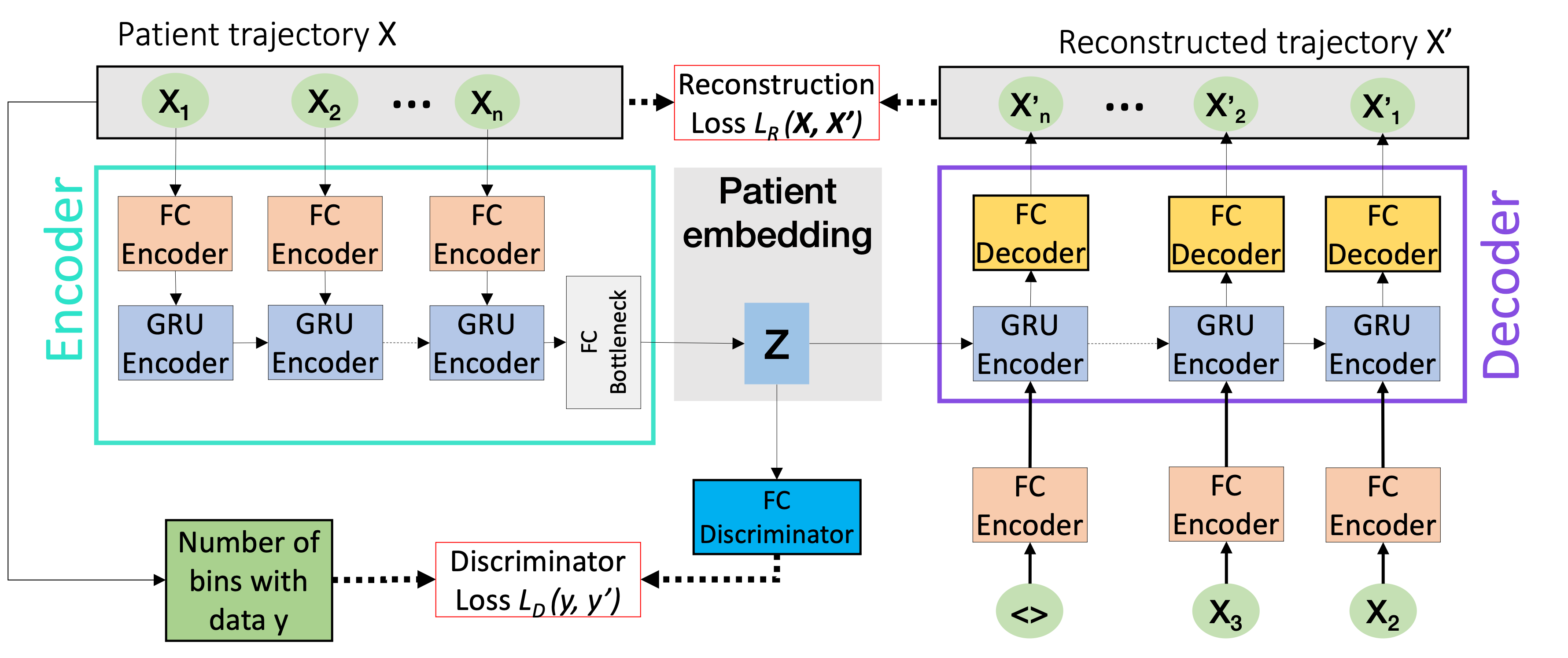
Figure 2: Illustration of the aGRU model. A GRU autoencoder model is extended by a discriminator loss $L_{D}$ to compensate the impact of the trajectory bias within the patient embedding $Z$. (FC - fully connected layer)

3.2 Models

Learning a temporal patient embedding. Our proposed adversarial gated recurrent neural network (aGRU) model is illustrated in Figure 2 and is based on a standard RNN-AE architecture, which was further extended by an adversarial training scheme as proposed in [16]. The encoder consists of a feature embedding layer which transforms the features of time window $\textbf{x}_{i}$ into a fixed-sized embedded vector of $256$ dimensions using a fully connected (FC) layer with ReLU activation function. The embedded time windows are passed into a bidirectional GRU layer, finally the last hidden state is feed into a bottle neck fully connected layer which transforms the sequential data into a patient embedding $z$ with an dimension of $n_{z}\,=\,256$. The decoder consists of a unidirectional GRU model followed by a FC feature decoder layer which reconstructs the trajectory $\textbf{X}^{\prime}$. The AE model is learned by minimising the reconstruction loss $L_{R}$ which is defined as:

$$L_{R}(\boldsymbol{X},\boldsymbol{X^{\prime}})=w_{b}*L_{bin}+L_{cont}$$ (1)

where $L_{bin}$ and $L_{cont}$ are the loss functions for the binary and continuous features and $w_{b}$ is a constant. Empirical results indicated that a good reconstruction performance for both, binary and continuous data, can be achieved by weighting the binary loss terms by $w_{b}=100$. Both losses use mean squared error (MSE) to calculate the error as follows:

$$L_{bin/cont}=\frac{1}{N}\sum_{i\in W_{T}}\sum_{j\in F_{bin/cont}}(\boldsymbol{X}(i,j)-\boldsymbol{X^{\prime}}(i,j))^{2}$$ (2)

where $N$ is the total elements used in the summation, $W_{T}$ refers to the windows inside the sequence that contains data (patient trajectory windows), and $F_{bin/cont}$ are the indices of the binary or continuous features respectively. Additionally, for $L_{cont}$ all the masked missing values where $\boldsymbol{X^{\prime}}(i,j)<0$ are excluded as well. We refer to this model, without the adversarial training scheme, as the GRU model.

To compensate the impact of the trajectory bias, this model is extended by an adversarial training scheme. The patient embedding $z$ is additionally connected to a FC discriminator layer which predicts the number of time windows with data which is optimized by

$$L_{D}=\frac{1}{N}(n_{w}-n_{w}^{\prime})^{2}$$ (3)

where $n_{w}$ is fraction of windows with data within a sequence (trajectory length over sequence length), and $n^{\prime}_{w}$ is the discriminator layer prediction.

The autoencoder loss is then modified as

$$L^{\prime}_{R}=L_{R}-\alpha\,*\,min(\beta,L_{D})$$ (4)

with $\alpha$ being a weighting parameter to control the impact of the adversarial training scheme, and $\beta$ is a threshold to cap the influence of $L_{D}$ once it reaches a certain value. The discriminator ($L_{D}$) and autoencoder losses ($L^{\prime}_{R}$) are minimized sequentially using the Adam optimizer with a learning rate of $2\times 10^{-3}$ for the autoencoder and $2\times 10^{-4}$ for the discriminator, and a weight decay of $10^{-6}$ for both of them.

Our adversarial training approach is based on work by Ganin and colleagues [16] with the following modifications: 1) we use a regression task instead of a classification one, 2) we optimize the generator and discriminator in two separate steps instead of using a gradient reversal layer, 3) we use a fixed value for $\alpha$ for the whole training, and 4) we cap the discriminator influence as $min(\beta,L_{d})$ to stabilize the learning process.

The models were trained using 80% of the data of the wider cohort using the remainder for validation. The trained models were then used to extract the embedding on the specific cohort where the trajectories were aligned on the index event.

To further investigate the impact of the trajectory bias, we also implemented a tLSTM model as proposed by Yin and colleagues [4]. For this model we removed the windows without data from the input, and add as input the time difference between the remaining windows with data.

Patient clustering. In the second step, a clustering of the patients in the embedded space is performed. Different clustering algorithms can be used. For the purpose of demonstrating the trajectory bias effect on the clustering results we present the results of a simple k-means algorithm. Therefore, patient embedding $z$ was reduced to $6$ dimensions using principal component analysis (PCA), as k-means does not perform well in high dimensional spaces [17].

Figure 3: Visualization of the first two principal components of the embedding space for a a) normal GRU, b) tLSTM and c) aGRU autoencoder model. Each dot represents the embedding of a patient in the $wider$ cohort. The color coding indicates how many time windows of the specific patient trajectory contains any kind of data. The legend shows colors for a selected number of values from the full range of possible trajectory durations.

3.3 Evaluation

To quantify how much a given patient embedding is influenced by trajectory bias, we took the root mean squared error (RMSE) of the differences between the trajectory length for the patient of interest and the trajectory lengths of the nearest neighbors in the embedding space obtained using a K-nearest neighbors (k-NN) regression model. We also quantified the extent of trajectory bias in the embeddings by training a surrogate model to predict cluster assignments using only information regarding which time windows were present for patients in the cohort and then evaluating the precision scores. Details of both the k-NN error and the surrogate model method are given in appendix 9.

4 Results

Figure 4: Comparison of the patient embeddings using the HF cohort and the 3 trajectories: after-event, event-to-end, ALL for a normal GRU model and our proposed aGRU approach ($\alpha=1$). Color coding indicates number of time windows per patient with any type of data (trajectory length). The blue box in case of GRU model indicates a cluster of patients which were only admitted to the hospital for the acute HF episode. This group is stronger overlapping with other patients in case of the aGRU model.

Wider cohort evaluation: To investigate this effect independently of specific trajectories, we trained our proposed aGRU model on the $wider$ cohort and compared the results of the patient embeddings with a normal GRU and a tLSTM model. The models were trained using all 5 data types (primary and secondary diagnosis, procedures, medications and laboratory values). The continuous data is included using rank normalization. The adversarial training scheme was implemented using $\alpha=1$ and $\beta=0.01$.

Figure 3 shows a visualization of the first two dimensions of PCA of the embedding space for all three models. Each point represents a patient in the wider cohort. The color coding indicates the number of windows which contain any type of data per patient (trajectory length). The results indicate a strong correlation between trajectory length and the first principal components for the GRU and a tLSTM model, which confirms our hypothesis. Using our adversarial training scheme, the impact on the trajectory length can be reduced. We quantified our findings using our metric for local differences in trajectory length measured in the embedding space (see section 3.C). The k-NN error (calculated in the OUH wider cohort) was 0.99 (std = 0.05) for the GRU, 1.46 (std = 0.09) for the tLSTM and 2.78 (std = 0.12) for the aGRU. The increased value in the aGRU model is indicative of a reduced influence of trajectory length.

Smaller cohort evaluation: We further investigated the trajectory bias in the specific cohorts. For each hospital we evaluate the models trained on the corresponding wider cohort on the smaller patient subset defined by HF or stroke cohort. We aligned the patient trajectories to their index event using three trajectory types: AfE, E2E, ALL. For the HF cohort, the results were generated for different weighting parameters $\alpha$ and clipping parameter $\beta$ to investigate the impact on the embedding results. Additionally, a simple cluster analysis as described in sec 3.2.

Figure 4 shows the first two PCA axis of the learned embedding space for the different trajectories of the HF cohort. As in case of the wider cohort analysis, the trajectory bias effect is clearly visible in case of the GRU model. The extent to which the embedding model was biased by the input trajectory lengths was again quantified using k-NN error (see section 3.C). The k-NN error values (calculated in the OUH HF cohort) for the GRU were 1.44 (std = 0.02), 1.23 (std = 0.01) and 2.48 (std = 0.01) for the AfE, E2E, and ALL trajectories respectively. For the aGRU model the k-NN error values were 2.94 (std = 0.03), 2.19 (std = 0.05) and 3.13 (std = 0.01) for the AfE, E2E, and ALL trajectories respectively. Again, the increased values for the aGRU model are indicative of a reduced influence of trajectory length. Note that the values obtained in the HF sample were larger than the values obtained in the wider cohort due to the reduced number of patients. Similar results were obtained for the other cohorts analyzed and are summarized in the appendix 10.

For instance in case of E2E trajectory, a clearly separable group of patients with very low number can be identified (marked by the blue box). These patients have only a single time window with data, indicating that they got only admitted for the acute HF event to the hospital and were further treated in a different facility. The trajectory bias can be compensated using the proposed adversarial training scheme (see lower row of the plots). As a result for the E2E trajectory embeddings, the before mentioned group of HF patients with a single time window is stronger overlapping with patients with longer trajectories.

Figure 5: Comparison of the embedding space using different weighting factors $\alpha$ for the after-event trajectory of the OUH HF cohort. Color coding indicates the number of time windows with data per patient.

The impact of the adversarial training can be adjusted by hyperparameter $\alpha$ (see Equation 4) which serves as a weighting parameter. The effect on the patient embedding space is visualized for $\alpha=\{0.1,\,1,\,10\}$ and compared to a normal GRU model for the AfE trajectory. Similar results were found for the other trajectories. It can be observed from the patient embedding plots in Figure 5 that the trajectory bias decreases as the value of $\alpha$ increases. This effect can also be seen by looking at the calculated k-NN error values for the different alpha values (see section 3.C). The k-NN error (calculated for the AfE trajectory in the HF cohort) for the GRU was 1.44 (std = 0.02), while the values calculated for the aGRU models were 2.69 (std = 0.02), 3.14 (std = 0.04) and 3.18 (std = 0.02) for $\alpha=0.1$, $\alpha=1$ and $\alpha=10$ respectively.

Initial results using the adversarial training scheme as proposed by Ganin and colleagues [16], resulted in an unstable training due to high gradients caused by $L_{adv}$. To compensate this effect, we constrained the adversarial training impact using $\beta$ (see Equation 4. Our results indicate that a learning is possible using a $\beta=\{0.1,\,0.01\}$. The parameter $\beta$ was set to $0.01$ for all results using aGRU. An alternative solution to this problem is the clipping of gradients.

How strong the trajectory bias should be compensated strongly depends on the specific clinical question and dataset. One way of determining how the $\alpha$ and $\beta$ values should be tuned is through evaluation of performance on a relevant downstream task.

The influence of the trajectory bias on potential patient clusters was further evaluated using a k-means cluster algorithm. As an example, the clustering was performed with $k=6$ clusters. The cluster results, visualized in the embedding space, for the OUH HF cohort are shown in top row of Figure 6. The box plots below show the distribution of the number of time windows per cluster. In case of the clustering results using the GRU model, it can be observed that the cluster $3$ only focuses on patients with a very short trajectory and in contrary cluster $2$ and $4$ on patient with a long trajectory. The difference between the clusters is strongly compensated using the aGRU approach.

A further quantification of the adversarial training scheme was performed by using surrogate prediction approach as described in section 3.C. Table I shows the averaged precision values for predicting the cluster assignment given the number of time windows with data for different values of $\alpha$ and trajectories. The average precision scores are higher for the E2E trajectory due to presence of patients with only a single time window with data, as discussed in the context of Figure 4.

5 Discussion

The results presented within the previous section indicate the impact of the trajectory bias for different methods, cohorts and trajectories. As shown in Figure 4, a typical GRU implementation as well as a tLSTM approach are effected. In case of the latter, the time difference between time windows is directly included in the RNN-AE model. For instance, if a patient has only data in the first quarter of 2016 and in the third quarter of 2019 the input sequence will have two elements, empty time windows in-between will be ignored. By contrast the GRU model input will have a fix sequence size of 22 where all the empty time windows are filled with the empty admission vector. This results in an decreased trajectory bias (indicated by the higher k-NN error value of $1.46$ compared to $1.08$ for the GRU model). Nonetheless, the trajectory bias remains present as patients with more data will result in a longer input sequence. This becomes visible in Figure 3.b as the first two principle components of the patient embeddings $z$ are highly correlated to the trajectory length (see Figure 2). Our proposed adversarial training scheme approach can compensate this effect. This is visually confirmed in Figure 3.c and Figure 4 (which are limited to only the first two principle components of the embedding space) as well as quantitatively with the k-NN error and surrogate model (see Table V in appendix 10). Please note, the adversarial training scheme is not limited to a GRU model and could also be applied to the tLSTM approach.

Figure 6: Top row: k-means clustering results on the patient embedding and bottom row: box plot of distribution of number of windows with data per cluster using either a a) GRU or b) aGRU autoencoder model.

Model	AfE	E2E	All
GRU	0.44±0.03	0.64±0.03	0.49±0.04
aGRU ($\alpha=0.1$)	0.38±0.04	0.57±0.02	0.41±0.03
aGRU ($\alpha=1$)	0.34±0.05	0.55±0.03	0.40±0.05
aGRU ($\alpha=10$)	0.30±0.04	0.37±0.02	0.40±0.04

Table 1: Average precision scores of a surrogate model to predict the cluster assignment (derived using k-means clustering) on the OUH HF cohort for different trajectories: AfE, E2E, and ALL for different AE models. Lower values here indicate that the embedding model has a reduced trajectory bias.

Our objective is that by compensation of the trajectory bias, an unsupervized phenotyping approach is more likely to find patient clusters which are determined by specific clinical observations rather when only the trajectory length. However, we emphasize that the knowledge of how much data is available in a patient trajectory is an important information in general. A healthy patient will be admitted less frequent to the hospital and vice versa. Nonetheless, there are various non-health related reasons, why a patient has less data. This could include reasons such as the patient moved to a different place, different ways of working between wards or modification of the hospital IT infrastructure. As these reasons are often unknown, we want to limit the impact of the trajectory length on the patient embedding.

How strong the trajectory bias should be compensated depends on the specific application. We explored the parameter $\alpha$ which serves as a weighting parameter to compensate the trajectory bias (see Figure 6 and Table I). It needs to be further investigated if there are some generic measures to supports the optimization of $\alpha$ to reduce the burden of clinicians to evaluate large number of cluster results.

Another aspect, which was not further explored into detail is the density of data points within a time window. The patient trajectory is transformed into an input sequence consisting of non overlapping time windows of 3 months. More granular information is only provided to the model for continuous data (number of tests in a given time window is computed) and in form of two administrative features, indicating the number of admissions and percentage of days in hospital. However in case of binary data, the model does not know if e.g. only one or multiple MRI scans (procedure code) were performed. This is of course also an indication of the severity of medical condition, which should be explored further and its relationship to the trajectory bias.

6 Conclusion

We showed that patient embeddings using previously proposed RNN-AE models are impacted by a trajectory bias, meaning that embeddings are heavily dependent on the amount of data contained in each patients trajectory, likely at the expense of clinically relevant details. We presented a novel method to overcome unwanted trajectory bias using an adversarial training scheme on top of a RNN-AE. We demonstrated that our approach was effective in different datasets, cohorts and a range of different patient trajectory types, with our results showing that we were able to flexibly reduce the extent of trajectory bias in our model.

7 Statistical description of cohorts and trajectories

An overview of the considered cohorts and trajectories for are shown in Table II for OUH and Table III for ChelWest. The number of patients are reported for the wider cohort, as well as the three different trajectories for both the HF and stroke cohort. For each of the feature types in the dataset, the mean number of that feature present per patient are also reported. Finally, a number of summary statisticals are reported for the trajectory durations.

Table 2: Statistical description of used cohorts and trajectories for OUH. # refers to the number of patients or features for the different data types present in the EHR data.

	$wider$	HF cohort			Stroke cohort
	cohort	E2E	AfE	All	E2E	AfE	All
Number of patients	493512	1430	1097	1430	1480	1035	1480
Data per patient Mean (Median):
Primary Diag.	0.96 (0)	3.77 (3)	2.72 (1)	5.93 (5)	3.01 (2)	2.21 (1)	5.15 (4)
Secondary Diag.	4.38 (1)	26.51 (18)	19.61 (10)	37.5 (27)	21.79 (15)	14.97 (7)	32.41 (23)
Procedures	3.05 (1)	7.10 (5)	5.65 (3)	12.48 (10)	7.88 (6)	4.37 (2)	13.15 (11)
Medications	8.38 (2)	33.42 (22)	23.91 (12)	49.60 (37)	28.83 (20)	18.59 (5)	44.99 (32)
Laboratory Values	71.55 (43)	91.81 (67.5)	88.76 (67)	202.28 (192)	78.44 (56)	78.90 (60)	182.93 (170)
Time windows with data:
Mean	5.16	5.15	5.41	12.46	4.32	4.74	11.29
Median	4	4	4	12	3	4	11
Min	1	1	1	1	1	1	1
Max	22	20	19	23	19	18	22

Table 3: Statistical description of used cohorts and trajectories ChelWest. # refers to the number of patients or features for the different data types present in the EHR data.

	$wider$	HF cohort			Stroke cohort
	cohort	E2E	AfE	All	E2E	AfE	All
Number of patients	129852	818	566	818	668	429	668
Data per patient Mean (Median):
Primary Diag.	1.72 (1)	3.84 (3)	2.93 (2)	6.08 (5)	2.79 (2)	2.17 (1)	5.15 (4)
Secondary Diag.	10.48 (5)	34.69 (24)	30.07 (20)	48.51 (38)	29.28 (19)	24.39 (15)	44.66 (32)
Procedures	7.78 (5)	8.68 (6)	7.31 (5)	16.22 (13)	7.72 (6)	5.70 (3)	16.31 (12)
Medications	6.45 (2)	21.15 (14)	17.00 (9)	29.68 (21)	19.48 (13)	14.21 (7)	29.42 (21)
Laboratory Values	86.62 (52)	110.53 (76)	105.26 (75)	211.67 (174)	83.97 (60)	73.97 (50)	186.92 (142)
Time windows with data:
Mean	4.84	4.19	4.61	9.08	3.25	3.51	8.18
Median	3	3	4	8	2	3	7
Min	1	1	1	1	1	1	1
Max	28	22	21	27	19	18	27

8 Inclusion and exclusion criteria for patients with a first acute heart-failure event

This event was defined as the occurrence of any of the following ICD-10 codes as a primary diagnosis: (i) I50* Heart failure, (ii) I11.0 Hypertensive heart disease with (congestive) heart failure, (iii) I13.0 Hypertensive heart and renal disease with (congestive) heart failure or (iv) I13.2 Hypertensive heart and renal disease with both (congestive) heart failure and renal failure. In addition to having one of these diagnoses, patients were only included in the cohort if they had at least 3 months of data available prior to the first admission where one of these diagnosis codes were recorded. Finally, we excluded patients from the cohort based on the following criteria: (i) patients whose first admission (as defined above) was under 48 hours and had a heart failure related procedure code in the 30 days following the first admission (OPCS-4 codes: K59*, K60*, K61*, K72*, K73*, K74*), (ii) patients who had heart failure related ICD-10 codes recorded as a secondary diagnoses prior to their first admission (ICD-10 codes: I50*, I11.0, I13.0, I13.2), (iii) patients who had been prescribed Eplerenone, Sacubitril with Valsartan or Spironolactone at a dose of either 25mg or 50mg, (iv) patients with a recorded New York Heart Association classification or (v) patients with a recorded ejection fraction under 40%.

9 Details for evaluation methods

K-nearest neighbors error: To quantify the extent to which a learned patient embedding is locally influenced by the trajectory bias, we calculated the RMSE between the trajectory lengths and the prediction of a k-NN regression model for a sample of patients. This gives a measure of the amount of variation there is in trajectory lengths between patients that are close to each other within the embedding space. For a given embedding space we will refer to this metric as the k-NN error. The full process consisted of the following steps: first we sampled $N$ random patients from a given cohort, then for a given patient, $i$, we find its $K$ nearest neighbors based on their Euclidean distance within the embedding space. The mean trajectory length for the nearest neighbors, $T_{kNN}$, was then calculated as,

$$T_{kNN_{i}}=\frac{1}{K}\sum\limits_{k=1}^{K}{T_{k,i}}$$ (5)

where $T_{k,i}$ refers to the trajectory length (time windows with any type of data a long the sequence) for the $k_{t}h$ nearest neighbor of patient $i$. The final k-NN error is calculated by taking the root of the mean of the squared differences between the k-NN predictions and the length for all the patients in the sample as

$$kNN_{error}=\sqrt{\frac{1}{N}\sum\limits_{i=1}^{N}{(T_{kNN_{i}}-T_{i})^{2}}}$$ (6)

For the results presented here, we used $N=1000$ and $K=5$. Increased influence of trajectory length in the embedding model will result in lower k-NN error values. To allow for us to obtain the standard deviation of this measure, each time the k-NN error was reported we calculated the value 10 times (obtaining new samples each time) and reported the mean and standard deviation across these 10 values.

Surrogate models: We used a further metric to investigate the impact of the trajectory bias on identified patient clusters. Patient trajectory data were converted to simple binary vectors that indicated whether or not a patient had any data for a specific time window. These binary vectors were used as inputs for a simple random forest classifier which was trained to predict the cluster labels assigned to patients by one of the investigated methods. The average precision scores were used to determine how well the surrogate model could predict the cluster labels using only information of the trajectory length. A lower trajectory bias in the identified patient clusters is indicated by a low average precision score.

10 Summary of the adversarial approach for all the different datasets.

Trust	Disease	Model	AfE	E2E	All
Hospital 1	HF	GRU	0.45±0.03	0.63±0.03	0.49±0.06
		aGRU	0.36±0.05	0.54±0.02	0.41±0.04
Hospital 1	Stroke	GRU	0.42±0.02	0.70±0.03	0.54±0.01
		aGRU	0.37±0.03	0.62±0.02	0.49±0.04
Hospital 2	HF	GRU	0.38±0.05	0.60±0.03	0.39±0.04
		aGRU	0.29±0.04	0.41±0.03	0.34±0.03
Hospital 2	Stroke	GRU	0.38±0.05	0.47±0.04	0.41±0.04
		aGRU	0.24±0.06	0.40±0.03	0.36±0.02

Table 4: Average precision scores of a surrogate model to predict the cluster assignment (derived using k-means clustering) for different trajectories: AfE, E2E, and ALL for different AE models. Lower values here indicate that the embedding model has a reduced trajectory bias.

Trust	Disease	Model	AfE	E2E	All
Hospital 1	HF	GRU	1.44±0.02	1.23±0.01	2.48±0.02
		aGRU	2.94±0.04	2.19±0.05	3.13±0.01
Hospital 1	Stroke	GRU	1.23±0.03	0.93±0.02	2.31±0.02
		aGRU	2.92±0.05	1.71±0.04	2.95±0.03
Hospital 2	HF	GRU	1.35±0.06	1.24±0.03	2.53±0.04
		aGRU	2.14±0.07	1.91±0.05	3.31±0.02
Hospital 2	Stroke	GRU	1.14±0.04	0.99±0.05	2.36±0.08
		aGRU	1.88±0.04	1.63±0.07	3.43±0.04

Table 5: Average k-Nearest neighbor error values for different trajectories: AfE, E2E, and ALL for different AE models. Higher values indicate that the embedding model has a reduced trajectory bias.

References

- [1] S. R. Evans et al., “Real-World Data for Planning Eligibility Criteria and Enhancing Recruitment: Recommendations from the Clinical Trials Transformation Initiative,” Therapeutic Innovation and Regulatory Science, 2021.
- [2] J. M. Banda et al., “Advances in Electronic Phenotyping: From Rule-Based Definitions to Machine Learning Models,” Annual Review of Biomedical Data Science, vol. 1, 2018.
- [3] I. M. Baytas et al., “Patient subtyping via time-aware LSTM networks,” in Proceedings of the ACM SIGKDD International Conference on Knowledge Discovery and Data Mining, 2017.
- [4] C. Yin et al., “Identifying Sepsis Subphenotypes via Time-Aware Multi-Modal Auto-Encoder,” in Proceedings of the ACM SIGKDD International Conference on Knowledge Discovery and Data Mining, 2020.
- [5] J. Zhang et al., “Patient2Vec: A Personalized Interpretable Deep Representation of the Longitudinal Electronic Health Record,” 2018.
- [6] C. Lee et al., “Temporal phenotyping using deep predictive clustering of disease progression,” in 37th International Conference on Machine Learning, ICML 2020, 2020.
- [7] Y. Kim et al., “Temporal phenotyping for transitional disease progress: An application to epilepsy and Alzheimer’s disease,” Journal of Biomedical Informatics, 2020.
- [8] A. Afshar et al., “TASTE: Temporal and Static Tensor Factorization for Phenotyping Electronic Health Records,” Proceedings of the ACM Conference on Health, Inference, and Learning, 2020.
- [9] B. K. Beaulieu-Jones et al., “Semi-supervised learning of the electronic health record for phenotype stratification,” Journal of Biomedical Informatics, 2016.
- [10] E. Choi et al., “Medical Concept Representation Learning from Electronic Health Records and its Application on Heart Failure Prediction,” 2016.
- [11] ——, “Multi-layer Representation Learning for Medical Concepts,” 2016.
- [12] L. Metz, J. Sohl-Dickstein, N. Maheswaranathan, and B. Cheung, “Meta-learning update rules for unsupervised representation learning,” in 7th International Conference on Learning Representations, ICLR 2019, 2019.
- [13] D. J. Trosten, A. S. Strauman, M. Kampffmeyer, and R. Jenssen, “Recurrent deep divergence-based clustering for simultaneous feature learning and clustering of variable length time series,” ieeexplore.ieee.org, 2019. [Online]. Available: https://ieeexplore.ieee.org/abstract/document/8682365/
- [14] D. Lenco and R. Interdonato, “Deep Multivariate Time Series Embedding Clustering via Attentive-Gated Autoencoder,” in Lecture Notes in Computer Science (including subseries Lecture Notes in Artificial Intelligence and Lecture Notes in Bioinformatics). Nature Publishing Group, 2020, pp. 318–329.
- [15] X. Qiu, H. Wu, and R. Hu, “The impact of quantile and rank normalization procedures on the testing power of gene differential expression analysis,” BMC Bioinformatics, 2013.
- [16] Y. Ganin et al., “Domain-adversarial training of neural networks,” Journal of Machine Learning Research, 2016.
- [17] C. C. Aggarwal, A. Hinneburg, and D. A. Keim, “On the surprising behavior of distance metrics in high dimensional space,” in International conference on database theory. Springer, 2001, pp. 420–434.